Dynamic variability of the Asian monsoon anticyclone ... and Randel 2013.pdfGARNY AND RANDEL: ANTICYCLONE VARIABILITY Figure 3. (a) PV at 360K and at 90ıE as a function of latitude

JOURNAL OF GEOPHYSICAL RESEARCH: ATMOSPHERES, VOL. 118, 13,421–13,433, doi:10.1002/2013JD020908, 2013

Dynamic variability of the Asian monsoon anticyclone observedin potential vorticity and correlations with tracer distributionsH. Garny1 and W. J. Randel2

Received 18 September 2013; revised 3 December 2013; accepted 3 December 2013; published 20 December 2013.

[1] The Asian summer monsoon is associated with strong upward transport oftropospheric source gases and isolation of air within the upper tropospheric anticyclone,with a high degree of dynamical variability. Here we study the anticyclone in terms ofpotential vorticity (PV) as derived from reanalysis data. The strength of the anticyclone,as measured by low PV area, varies on subseasonal time scales (periods of 30–40 days),driven by variability in convection. The convective forcing of low PV areas is associatedwith heating in the middle troposphere and divergent motion in the upper troposphere,and we find that upper level divergence is a good predictor of the anticyclone strength.Low PV air is often observed to propagate from the forcing region to the west, andoccasionally to the east. Carbon monoxide (CO) measured by the Aura Microwave LimbSounder is used to study the covariability of chemical tracers with the anticyclonestrength and location. Concentrations of CO maximize within the upper troposphericanticyclone, and enhanced CO is well correlated with the spatial distribution of low PV.Time variations of CO concentrations in the upper troposphere (around 360 K) are notstrongly correlated with anticyclone strength, probably because CO transport alsoinvolves coupling with surface CO sources (unlike PV). Temporal correlations with PVare stronger for CO at higher levels (380–400 K), suggesting that advective upwardtransport is important for tracer evolution at these levels.Citation: Garny, H., and W. J. Randel (2013), Dynamic variability of the Asian monsoon anticyclone observed in potentialvorticity and correlations with tracer distributions, J. Geophys. Res. Atmos., 118, 13,421–13,433, doi:10.1002/2013JD020908.

1. Introduction[2] In response to persistent convection associated with

the Asian summer monsoon, a large-scale anticyclone occursin the upper troposphere and lower stratosphere (UTLS).The strong circulation of the anticyclone acts to isolate air,and because this isolated air is tied to the outflow of deepconvection, the anticyclone often has a distinct chemical sig-nature [Dethof et al., 1999; Randel and Park, 2006; Parket al., 2007, 2008; Baker et al., 2011]. The UTLS anticy-clone is a seasonal feature, beginning in June and ending inSeptember. The evolution over the season is characterizedby large variability in the extent, strength, and location of theanticyclone [Randel and Park, 2006]. Oscillations with peri-ods of 10–20 and 30–60 days were found by Annamalai andSlingo [2001], and they concluded that these are driven byvariations in the monsoon convection. Zhang et al. [2002]found that the location of the center of the anticycloneat 100 hPa is bimodal and classified a Tibetan Mode and

1Deutsches Zentrum für Luft- und Raumfahrt, Institut für Physik derAtmosphäre, Oberpfaffenhofen, Germany.

2National Center for Atmospheric Research, Boulder, Colorado, USA.

Corresponding author: H. Garny, Deutsches Zentrum für Luft- undRaumfahrt, Institut für Physik der Atmosphäre, DE-82234 Oberpfaffen-hofen, Germany. ([email protected])

©2013. American Geophysical Union. All Rights Reserved.2169-897X/13/10.1002/2013JD020908

Iranian Mode according to the location of the center. Asso-ciated with these modes, Yan et al. [2011] found traceranomalies that are shifted in longitude depending on thelocation of the anticyclone. Less detail is known of subsea-sonal variations in tracers and their links with dynamicalvariability of the anticyclone on smaller spatial scales.

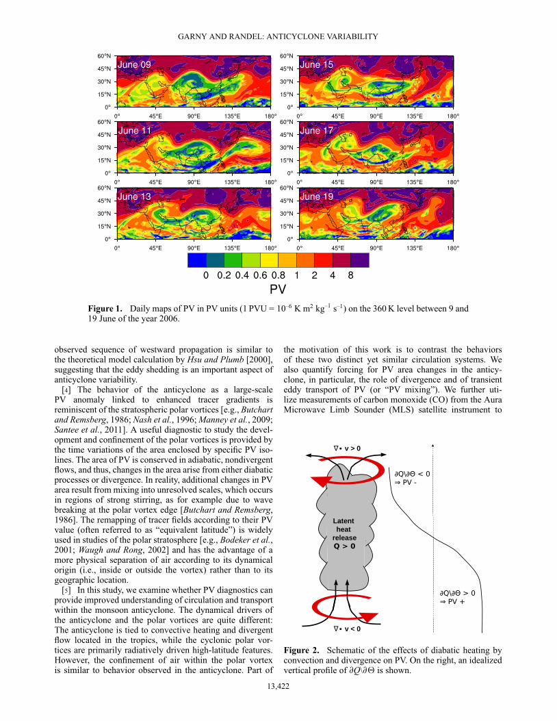
[3] Linear models closely reproduce the climatologicalfeatures of the anticyclone as wave response to diabaticheating [Gill, 1980; Hoskins and Rodwell, 1995]. However,as pointed out by Plumb [2007], these linear theories arenot consistent with the simple balances of uniform angu-lar momentum in the Hadley cell, and eddy transports andinstability are fundamental aspects of the upper tropospherevorticity balance (see also Sardeshmukh and Held [1984]).Hsu and Plumb [2000] show with an idealized nonlinearmodel that the response to divergent flow under conditionsrepresentative of the real atmosphere becomes unstable, andeddy transport of potential vorticity (PV) by “eddy shed-ding” from the anticyclone occurs. Hsu and Plumb [2000]and Popovic and Plumb [2001] show evidence of eddy shed-ding from observations. Figure 1 shows an example of thedynamic variability of the anticyclone over 9–19 June 2006viewed in terms of potential vorticity (PV). The anticy-clone is a region of low PV, and this sequence highlightsfine-scale structure and propagation of low PV air both tothe east and to the west of the anticyclone center, coinci-dent with weakening of the anticyclone. In particular, the

13,421

GARNY AND RANDEL: ANTICYCLONE VARIABILITY

Figure 1. Daily maps of PV in PV units (1 PVU = 10–6 K m2 kg–1 s–1) on the 360 K level between 9 and19 June of the year 2006.

observed sequence of westward propagation is similar tothe theoretical model calculation by Hsu and Plumb [2000],suggesting that the eddy shedding is an important aspect ofanticyclone variability.

[4] The behavior of the anticyclone as a large-scalePV anomaly linked to enhanced tracer gradients isreminiscent of the stratospheric polar vortices [e.g., Butchartand Remsberg, 1986; Nash et al., 1996; Manney et al., 2009;Santee et al., 2011]. A useful diagnostic to study the devel-opment and confinement of the polar vortices is provided bythe time variations of the area enclosed by specific PV iso-lines. The area of PV is conserved in adiabatic, nondivergentflows, and thus, changes in the area arise from either diabaticprocesses or divergence. In reality, additional changes in PVarea result from mixing into unresolved scales, which occursin regions of strong stirring, as for example due to wavebreaking at the polar vortex edge [Butchart and Remsberg,1986]. The remapping of tracer fields according to their PVvalue (often referred to as “equivalent latitude”) is widelyused in studies of the polar stratosphere [e.g., Bodeker et al.,2001; Waugh and Rong, 2002] and has the advantage of amore physical separation of air according to its dynamicalorigin (i.e., inside or outside the vortex) rather than to itsgeographic location.

[5] In this study, we examine whether PV diagnostics canprovide improved understanding of circulation and transportwithin the monsoon anticyclone. The dynamical drivers ofthe anticyclone and the polar vortices are quite different:The anticyclone is tied to convective heating and divergentflow located in the tropics, while the cyclonic polar vor-tices are primarily radiatively driven high-latitude features.However, the confinement of air within the polar vortexis similar to behavior observed in the anticyclone. Part of

the motivation of this work is to contrast the behaviorsof these two distinct yet similar circulation systems. Wealso quantify forcing for PV area changes in the anticy-clone, in particular, the role of divergence and of transienteddy transport of PV (or “PV mixing”). We further uti-lize measurements of carbon monoxide (CO) from the AuraMicrowave Limb Sounder (MLS) satellite instrument to

Figure 2. Schematic of the effects of diabatic heating byconvection and divergence on PV. On the right, an idealizedvertical profile of @Q\@‚ is shown.

13,422


Figure 3. (a) PV at 360 K and at 90ıE as a function of latitude for 3 days of the year 2006: 20 May(solid), 14 July (dashed), and 30 September (dotted). (b) Same as Figure 3a but PV in area coordinates(or equivalent latitude, with the lowest PV moved to the pole). The area is calculated in the domain15ıN–45ıN and 0ıE–180ıE and is given in relative units (the area of the whole domain is 1.0). (c) Areaof PV for the polar vortex at 850 K for 15 November of the year 2005 (solid), 1 January (dashed), and28 February (dotted) of year 2006. Here, the area is calculated for the Northern Hemisphere polewardof 50ıN.

analyze tracer variability within the anticyclone and quantifylinks with PV.

2. Data[6] The analyses in this study are based on a combina-

tion of reanalysis data for dynamical quantities and satellitedata for trace gases. The Modern-Era Retrospective Analy-sis for Research and Applications (MERRA) reanalysis data[Rienecker et al., 2011] are used here for the years2005–2009. These data have high horizontal resolution(0.5ı latitude by 0.67ı longitude), with a 6-hourly temporalresolution. The wind and temperature fields are used to cal-culate potential vorticity on isentropic surfaces. CO data areobtained from the Aura Microwave Limb Sounder (MLS)instrument. MLS has been in operation since August 2004.Here, the Level 2 data of version 3.3 are used [Livesey et

al., 2011]. The vertical resolution of CO in the upper tro-posphere and lower stratosphere is about 4.5 km (5 km fortemperature). Retrievals of CO are centered on pressure lev-els of 215, 147, 100, and 68 hPa. The precision of CO datais given with 19, 15, and 14 ppb at 215, 147, and 100 hPa,respectively, and a systematic uncertainty of 30% and 30ppb is given by Livesey et al. [2011]. The screening of thedata was performed as suggested in Livesey et al. [2011],including scanning for ice water content. For most of theanalysis performed in this study, the CO data are used on thesatellite track, i.e., directly using values as retrieved fromthe satellite measurements. For maps of CO, daily grid-ded fields were constructed with a horizontal resolution of5ı latitude and 10ı longitude. We interpolate the CO datafrom pressure levels to potential temperature levels usingthe temperatures retrieved from MLS; these interpolated val-ues still represent an average over a broad layer rather thanspecific levels.

13,423


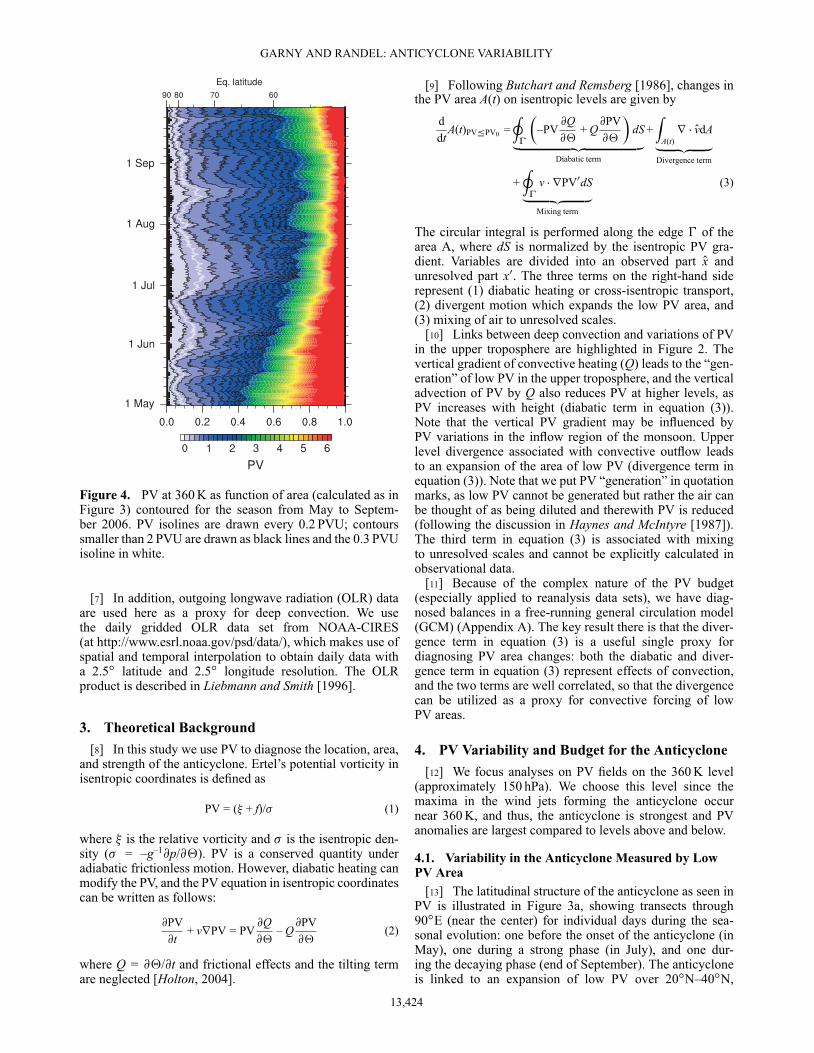
Figure 4. PV at 360 K as function of area (calculated as inFigure 3) contoured for the season from May to Septem-ber 2006. PV isolines are drawn every 0.2 PVU; contourssmaller than 2 PVU are drawn as black lines and the 0.3 PVUisoline in white.

[7] In addition, outgoing longwave radiation (OLR) dataare used here as a proxy for deep convection. We usethe daily gridded OLR data set from NOAA-CIRES(at http://www.esrl.noaa.gov/psd/data/), which makes use ofspatial and temporal interpolation to obtain daily data witha 2.5ı latitude and 2.5ı longitude resolution. The OLRproduct is described in Liebmann and Smith [1996].

3. Theoretical Background[8] In this study we use PV to diagnose the location, area,

and strength of the anticyclone. Ertel’s potential vorticity inisentropic coordinates is defined as

PV = (� + f)/� (1)

where � is the relative vorticity and � is the isentropic den-sity (� = –g–1@p/@‚). PV is a conserved quantity underadiabatic frictionless motion. However, diabatic heating canmodify the PV, and the PV equation in isentropic coordinatescan be written as follows:

@PV@t

+ vrPV = PV@Q@‚

– Q@PV@‚

(2)

where Q = @‚/@t and frictional effects and the tilting termare neglected [Holton, 2004].

[9] Following Butchart and Remsberg [1986], changes inthe PV area A(t) on isentropic levels are given by

ddt

A(t)PV�PV0 =I�

�–PV

@Q@‚

+ Q@PV@‚

�dS

„ ƒ‚ …Diabatic term

+Z

A(t)r � OvdA

„ ƒ‚ …Divergence term

+I�

v � rPV0dS„ ƒ‚ …

Mixing term

(3)

The circular integral is performed along the edge � of thearea A, where dS is normalized by the isentropic PV gra-dient. Variables are divided into an observed part Ox andunresolved part x0. The three terms on the right-hand siderepresent (1) diabatic heating or cross-isentropic transport,(2) divergent motion which expands the low PV area, and(3) mixing of air to unresolved scales.

[10] Links between deep convection and variations of PVin the upper troposphere are highlighted in Figure 2. Thevertical gradient of convective heating (Q) leads to the “gen-eration” of low PV in the upper troposphere, and the verticaladvection of PV by Q also reduces PV at higher levels, asPV increases with height (diabatic term in equation (3)).Note that the vertical PV gradient may be influenced byPV variations in the inflow region of the monsoon. Upperlevel divergence associated with convective outflow leadsto an expansion of the area of low PV (divergence term inequation (3)). Note that we put PV “generation” in quotationmarks, as low PV cannot be generated but rather the air canbe thought of as being diluted and therewith PV is reduced(following the discussion in Haynes and McIntyre [1987]).The third term in equation (3) is associated with mixingto unresolved scales and cannot be explicitly calculated inobservational data.

[11] Because of the complex nature of the PV budget(especially applied to reanalysis data sets), we have diag-nosed balances in a free-running general circulation model(GCM) (Appendix A). The key result there is that the diver-gence term in equation (3) is a useful single proxy fordiagnosing PV area changes: both the diabatic and diver-gence term in equation (3) represent effects of convection,and the two terms are well correlated, so that the divergencecan be utilized as a proxy for convective forcing of lowPV areas.

4. PV Variability and Budget for the Anticyclone[12] We focus analyses on PV fields on the 360 K level

(approximately 150 hPa). We choose this level since themaxima in the wind jets forming the anticyclone occurnear 360 K, and thus, the anticyclone is strongest and PVanomalies are largest compared to levels above and below.

4.1. Variability in the Anticyclone Measured by LowPV Area

[13] The latitudinal structure of the anticyclone as seen inPV is illustrated in Figure 3a, showing transects through90ıE (near the center) for individual days during the sea-sonal evolution: one before the onset of the anticyclone (inMay), one during a strong phase (in July), and one dur-ing the decaying phase (end of September). The anticycloneis linked to an expansion of low PV over 20ıN–40ıN,

13,424


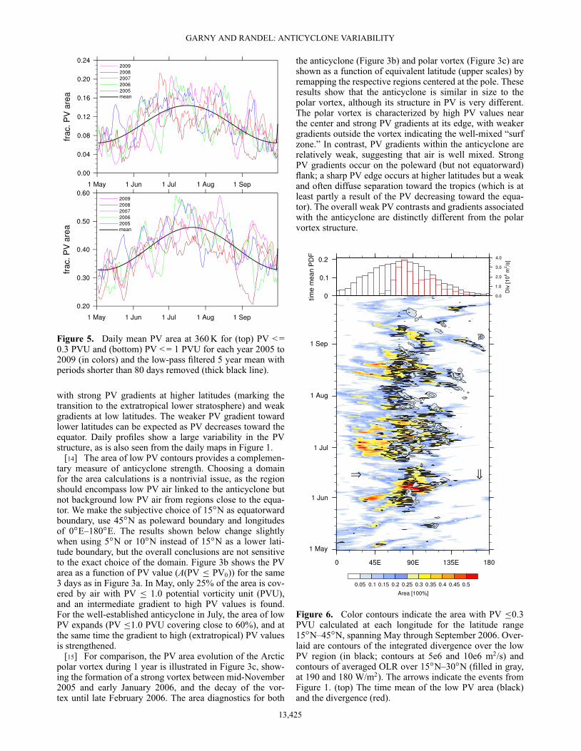
Figure 5. Daily mean PV area at 360 K for (top) PV < =0.3 PVU and (bottom) PV < = 1 PVU for each year 2005 to2009 (in colors) and the low-pass filtered 5 year mean withperiods shorter than 80 days removed (thick black line).

with strong PV gradients at higher latitudes (marking thetransition to the extratropical lower stratosphere) and weakgradients at low latitudes. The weaker PV gradient towardlower latitudes can be expected as PV decreases toward theequator. Daily profiles show a large variability in the PVstructure, as is also seen from the daily maps in Figure 1.

[14] The area of low PV contours provides a complemen-tary measure of anticyclone strength. Choosing a domainfor the area calculations is a nontrivial issue, as the regionshould encompass low PV air linked to the anticyclone butnot background low PV air from regions close to the equa-tor. We make the subjective choice of 15ıN as equatorwardboundary, use 45ıN as poleward boundary and longitudesof 0ıE–180ıE. The results shown below change slightlywhen using 5ıN or 10ıN instead of 15ıN as a lower lati-tude boundary, but the overall conclusions are not sensitiveto the exact choice of the domain. Figure 3b shows the PVarea as a function of PV value (A(PV � PV0)) for the same3 days as in Figure 3a. In May, only 25% of the area is cov-ered by air with PV � 1.0 potential vorticity unit (PVU),and an intermediate gradient to high PV values is found.For the well-established anticyclone in July, the area of lowPV expands (PV �1.0 PVU covering close to 60%), and atthe same time the gradient to high (extratropical) PV valuesis strengthened.

[15] For comparison, the PV area evolution of the Arcticpolar vortex during 1 year is illustrated in Figure 3c, show-ing the formation of a strong vortex between mid-November2005 and early January 2006, and the decay of the vor-tex until late February 2006. The area diagnostics for both

the anticyclone (Figure 3b) and polar vortex (Figure 3c) areshown as a function of equivalent latitude (upper scales) byremapping the respective regions centered at the pole. Theseresults show that the anticyclone is similar in size to thepolar vortex, although its structure in PV is very different.The polar vortex is characterized by high PV values nearthe center and strong PV gradients at its edge, with weakergradients outside the vortex indicating the well-mixed “surfzone.” In contrast, PV gradients within the anticyclone arerelatively weak, suggesting that air is well mixed. StrongPV gradients occur on the poleward (but not equatorward)flank; a sharp PV edge occurs at higher latitudes but a weakand often diffuse separation toward the tropics (which is atleast partly a result of the PV decreasing toward the equa-tor). The overall weak PV contrasts and gradients associatedwith the anticyclone are distinctly different from the polarvortex structure.

Figure 6. Color contours indicate the area with PV �0.3PVU calculated at each longitude for the latitude range15ıN–45ıN, spanning May through September 2006. Over-laid are contours of the integrated divergence over the lowPV region (in black; contours at 5e6 and 10e6 m2/s) andcontours of averaged OLR over 15ıN–30ıN (filled in gray,at 190 and 180 W/m2). The arrows indicate the events fromFigure 1. (top) The time mean of the low PV area (black)and the divergence (red).

13,425


Figure 7. (top) Time series from the year 2006 of daily mean low PV area with PV �0.3 PVU (black)together with integrated divergence over this area (blue) and mean OLR over 15ıN–30ıN and 60ıE–120ıE (red). (bottom) The 5 year mean (2005–2009) correlation (left) and optimal lag (right) of PV areawith divergence (blue) and OLR (red) as a function of PV threshold. The correlations are calculated foreach year over the deseasonalized time series from May to September.

[16] The seasonal evolution of the PV area in the anticy-clone region for the year 2006 is shown in Figure 4. The areaof low PV expands from May to about mid-July and retreatsafterward, and subseasonal variations in the strength of theanticyclone are superimposed on the seasonal changes. Thisseasonal behavior is found as well in other years, as shownin Figure 5 for five different years (2005–2009). The meanseasonal evolution (black line) shows the expansion of lowPV in June and decay in late August and September. Theseasonal mean evolution is calculated by applying a low-pass filter to the 5 year mean time series, removing periodssmaller than 80 days. This seasonal mean evolution is sub-tracted from time series when calculating correlations andpower spectra in the following (referred to as deseasonal-ized time series). Each year, the low PV areas exhibit strongintraseasonal variability, and this variability is stronger forareas of lower PV thresholds. The variability of the lowestPV isolines are a measure of the intensity of the circulation,and in the following we use the 0.3 PVU area to define thestrength of the anticyclone. Variations in higher PV thresh-olds are correlated with the 0.3 PVU area and lagged slightlyin time ( 1–3 days).

[17] The longitude-time variability of low PV air canbe depicted in a Hovmoller diagram, showing the areaof low PV (�0.3 PVU) as a function of longitude andtime (Figure 6). Low PV air is most often observed over

Figure 8. Correlation of low PV area (PV �0.3 PVU) ateach longitude with respect to the divergence term averagedover 70ıE–110ıE (indicated by the vertical dashed lines),calculated from data averaged over 2005–2009. The corre-lations are calculated for each year over the deseasonalizedtime series from May to September, with periods shorterthan 10 days removed from the time series. The dashedwhite lines give the timing of the maximum correlation ateach longitude.

13,426


longitudes 75ıE–90ıE, which we define as the center ofthe anticyclone. Low PV air is often observed to propagatefrom the center to the west in Figure 6 and occasionally tothe east. For example, the breaking event to the east thatwas seen in Figure 1 (9–11 June) is apparent as a stretchof low PV toward the east in early/middle June (indicatedby the arrow on the right). Likewise, the westward “rollingup” of PV isolines in the following days (13–17 June) isobserved as propagation of low PV area toward the west inmid-June (see arrow on left in Figure 6). As seen in Figure 1the low PV patch is eventually readvected toward the east,being captured in the westerly winds in the northern partof the anticyclone. This behavior is captured only weaklyin the Hovmoeller diagram: since the air is mixed with itssurrounding in the process, the low PV values are mixedtoward higher values which are not detected in the low PVarea diagnostic.

4.2. Drivers of Variability in Low PV Area[18] What drives the intraseasonal variability in the anti-

cyclone? The anticyclone is the upper tropospheric responseto diabatic heating by deep convection, and the intensity ofdeep convection varies over the season, so that the forc-ing of the anticyclone is itself highly variable. In addition,the dynamical instability of the anticyclone is predicted tolead to transience and periodic eddy shedding. Therefore, inaddition to the variability in the forcing, intrinsic dynamicvariability can be expected.

[19] Several previous studies have used area-averagedOLR as proxy for the convective influence on the anticy-clone [Randel and Park, 2006; Park et al., 2007]. Here, weuse the PV area equation (equation (3)) to investigate thephysical link between convection and the variability of theanticyclone. As discussed in section 3, both diabatic heat-ing due to convection and the divergence associated withthe convective outflow lead to increases in the area of lowPV. Calculations based on model simulations (Appendix A)suggest that the divergence and diabatic heating terms areclosely related, and for simplicity, we use the divergenceterm as a representation of the effects of convection on lowPV area.

[20] Figure 7 shows the time series of the area of lowPV (for the PV = 0.3 isoline) together with the mean OLRand the integrated divergence over the low PV area, thelatter representing the forcing of the anticyclone accord-ing to equation (3). The low PV area is highly correlatedwith the divergence term (correlation of 0.76), while cor-relations with OLR are weaker (0.37). For statistics overthe 5 years 2005–2009, the low PV area is matched bet-ter by the divergence term (correlation of 0.66) than byOLR (correlation of 0.38), as shown in Figure 7 (bot-tom). Correlations are calculated from deseasonalized timeseries (see discussion of Figure 5), in order to focus on theintraseasonal variability. The correlation of low PV area ishigher with divergence than with OLR for all PV thresh-olds used to calculate the PV area, but correlations are bestfor low PV values. The time lag for optimal correlationalso increases for higher values of PV, and this is consistentwith mixing low PV toward higher PV following convectiveevents, thereby expanding the area of larger PV thresholds.The correlation of the divergence forcing to the low PVarea demonstrates a direct physical link between convective

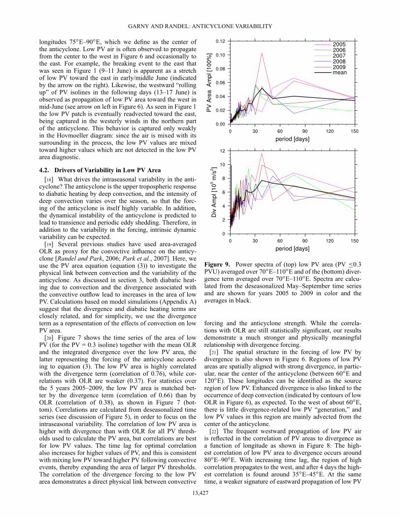
Figure 9. Power spectra of (top) low PV area (PV �0.3PVU) averaged over 70ıE–110ıE and of the (bottom) diver-gence term averaged over 70ıE–110ıE. Spectra are calcu-lated from the deseasonalized May–September time seriesand are shown for years 2005 to 2009 in color and theaverages in black.

forcing and the anticyclone strength. While the correla-tions with OLR are still statistically significant, our resultsdemonstrate a much stronger and physically meaningfulrelationship with divergence forcing.

[21] The spatial structure in the forcing of low PV bydivergence is also shown in Figure 6. Regions of low PVareas are spatially aligned with strong divergence, in partic-ular, near the center of the anticyclone (between 60ıE and120ıE). These longitudes can be identified as the sourceregion of low PV. Enhanced divergence is also linked to theoccurrence of deep convection (indicated by contours of lowOLR in Figure 6), as expected. To the west of about 60ıE,there is little divergence-related low PV “generation,” andlow PV values in this region are mainly advected from thecenter of the anticyclone.

[22] The frequent westward propagation of low PV airis reflected in the correlation of PV areas to divergence asa function of longitude as shown in Figure 8: The high-est correlation of low PV area to divergence occurs around80ıE–90ıE. With increasing time lag, the region of highcorrelation propagates to the west, and after 4 days the high-est correlation is found around 35ıE–45ıE. At the sametime, a weaker signature of eastward propagation of low PV

13,427


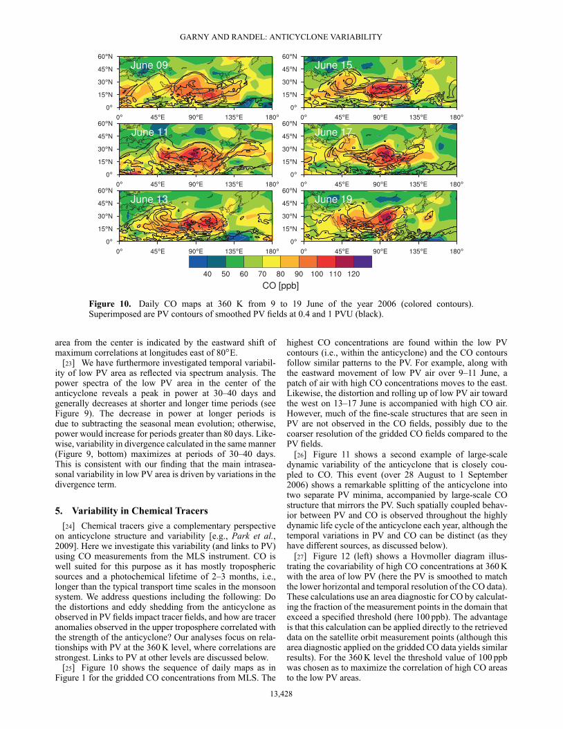
Figure 10. Daily CO maps at 360 K from 9 to 19 June of the year 2006 (colored contours).Superimposed are PV contours of smoothed PV fields at 0.4 and 1 PVU (black).

area from the center is indicated by the eastward shift ofmaximum correlations at longitudes east of 80ıE.

[23] We have furthermore investigated temporal variabil-ity of low PV area as reflected via spectrum analysis. Thepower spectra of the low PV area in the center of theanticyclone reveals a peak in power at 30–40 days andgenerally decreases at shorter and longer time periods (seeFigure 9). The decrease in power at longer periods isdue to subtracting the seasonal mean evolution; otherwise,power would increase for periods greater than 80 days. Like-wise, variability in divergence calculated in the same manner(Figure 9, bottom) maximizes at periods of 30–40 days.This is consistent with our finding that the main intrasea-sonal variability in low PV area is driven by variations in thedivergence term.

5. Variability in Chemical Tracers[24] Chemical tracers give a complementary perspective

on anticyclone structure and variability [e.g., Park et al.,2009]. Here we investigate this variability (and links to PV)using CO measurements from the MLS instrument. CO iswell suited for this purpose as it has mostly troposphericsources and a photochemical lifetime of 2–3 months, i.e.,longer than the typical transport time scales in the monsoonsystem. We address questions including the following: Dothe distortions and eddy shedding from the anticyclone asobserved in PV fields impact tracer fields, and how are traceranomalies observed in the upper troposphere correlated withthe strength of the anticyclone? Our analyses focus on rela-tionships with PV at the 360 K level, where correlations arestrongest. Links to PV at other levels are discussed below.

[25] Figure 10 shows the sequence of daily maps as inFigure 1 for the gridded CO concentrations from MLS. The

highest CO concentrations are found within the low PVcontours (i.e., within the anticyclone) and the CO contoursfollow similar patterns to the PV. For example, along withthe eastward movement of low PV air over 9–11 June, apatch of air with high CO concentrations moves to the east.Likewise, the distortion and rolling up of low PV air towardthe west on 13–17 June is accompanied with high CO air.However, much of the fine-scale structures that are seen inPV are not observed in the CO fields, possibly due to thecoarser resolution of the gridded CO fields compared to thePV fields.

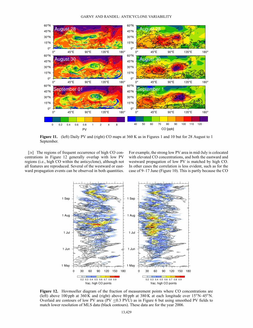
[26] Figure 11 shows a second example of large-scaledynamic variability of the anticyclone that is closely cou-pled to CO. This event (over 28 August to 1 September2006) shows a remarkable splitting of the anticyclone intotwo separate PV minima, accompanied by large-scale COstructure that mirrors the PV. Such spatially coupled behav-ior between PV and CO is observed throughout the highlydynamic life cycle of the anticyclone each year, although thetemporal variations in PV and CO can be distinct (as theyhave different sources, as discussed below).

[27] Figure 12 (left) shows a Hovmoller diagram illus-trating the covariability of high CO concentrations at 360 Kwith the area of low PV (here the PV is smoothed to matchthe lower horizontal and temporal resolution of the CO data).These calculations use an area diagnostic for CO by calculat-ing the fraction of the measurement points in the domain thatexceed a specified threshold (here 100 ppb). The advantageis that this calculation can be applied directly to the retrieveddata on the satellite orbit measurement points (although thisarea diagnostic applied on the gridded CO data yields similarresults). For the 360 K level the threshold value of 100 ppbwas chosen as to maximize the correlation of high CO areasto the low PV areas.

13,428


Figure 11. (left) Daily PV and (right) CO maps at 360 K as in Figures 1 and 10 but for 28 August to 1September.

[28] The regions of frequent occurrence of high CO con-centrations in Figure 12 generally overlap with low PVregions (i.e., high CO within the anticyclone), although notall features are reproduced. Several of the westward or east-ward propagation events can be observed in both quantities.

For example, the strong low PV area in mid-July is colocatedwith elevated CO concentrations, and both the eastward andwestward propagation of low PV is matched by high CO.In other cases the correlation is less evident, such as for thecase of 9–17 June (Figure 10). This is partly because the CO

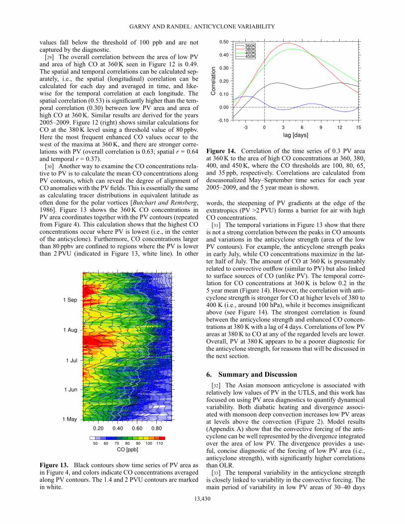
Figure 12. Hovmoeller diagram of the fraction of measurement points where CO concentrations are(left) above 100 ppb at 360 K and (right) above 80 ppb at 380 K at each longitude over 15ıN–45ıN.Overlaid are contours of low PV area (PV �0.3 PVU) as in Figure 6 but using smoothed PV fields tomatch lower resolution of MLS data (black contours). These data are for the year 2006.

13,429


values fall below the threshold of 100 ppb and are notcaptured by the diagnostic.

[29] The overall correlation between the area of low PVand area of high CO at 360 K seen in Figure 12 is 0.49.The spatial and temporal correlations can be calculated sep-arately, i.e., the spatial (longitudinal) correlation can becalculated for each day and averaged in time, and like-wise for the temporal correlation at each longitude. Thespatial correlation (0.53) is significantly higher than the tem-poral correlation (0.30) between low PV area and area ofhigh CO at 360 K. Similar results are derived for the years2005–2009. Figure 12 (right) shows similar calculations forCO at the 380 K level using a threshold value of 80 ppbv.Here the most frequent enhanced CO values occur to thewest of the maxima at 360 K, and there are stronger corre-lations with PV (overall correlation is 0.63; spatial r = 0.64and temporal r = 0.37).

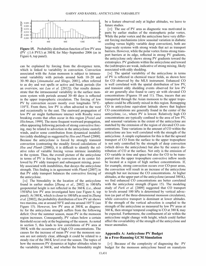
[30] Another way to examine the CO concentrations rela-tive to PV is to calculate the mean CO concentrations alongPV contours, which can reveal the degree of alignment ofCO anomalies with the PV fields. This is essentially the sameas calculating tracer distributions in equivalent latitude asoften done for the polar vortices [Butchart and Remsberg,1986]. Figure 13 shows the 360 K CO concentrations inPV area coordinates together with the PV contours (repeatedfrom Figure 4). This calculation shows that the highest COconcentrations occur where PV is lowest (i.e., in the centerof the anticyclone). Furthermore, CO concentrations largerthan 80 ppbv are confined to regions where the PV is lowerthan 2 PVU (indicated in Figure 13, white line). In other

Figure 13. Black contours show time series of PV area asin Figure 4, and colors indicate CO concentrations averagedalong PV contours. The 1.4 and 2 PVU contours are markedin white.

Figure 14. Correlation of the time series of 0.3 PV areaat 360 K to the area of high CO concentrations at 360, 380,400, and 450 K, where the CO thresholds are 100, 80, 65,and 35 ppb, respectively. Correlations are calculated fromdeseasonalized May–September time series for each year2005–2009, and the 5 year mean is shown.

words, the steepening of PV gradients at the edge of theextratropics (PV >2 PVU) forms a barrier for air with highCO concentrations.

[31] The temporal variations in Figure 13 show that thereis not a strong correlation between the peaks in CO amountsand variations in the anticyclone strength (area of the lowPV contours). For example, the anticyclone strength peaksin early July, while CO concentrations maximize in the lat-ter half of July. The amount of CO at 360 K is presumablyrelated to convective outflow (similar to PV) but also linkedto surface sources of CO (unlike PV). The temporal corre-lation for CO concentrations at 360 K is below 0.2 in the5 year mean (Figure 14). However, the correlation with anti-cyclone strength is stronger for CO at higher levels of 380 to400 K (i.e., around 100 hPa), while it becomes insignificantabove (see Figure 14). The strongest correlation is foundbetween the anticyclone strength and enhanced CO concen-trations at 380 K with a lag of 4 days. Correlations of low PVareas at 380 K to CO at any of the regarded levels are lower.Overall, PV at 380 K appears to be a poorer diagnostic forthe anticyclone strength, for reasons that will be discussed inthe next section.

6. Summary and Discussion[32] The Asian monsoon anticyclone is associated with

relatively low values of PV in the UTLS, and this work hasfocused on using PV area diagnostics to quantify dynamicalvariability. Both diabatic heating and divergence associ-ated with monsoon deep convection increases low PV areasat levels above the convection (Figure 2). Model results(Appendix A) show that the convective forcing of the anti-cyclone can be well represented by the divergence integratedover the area of low PV. The divergence provides a use-ful, concise diagnostic of the forcing of low PV area (i.e.,anticyclone strength), with significantly higher correlationsthan OLR.

[33] The temporal variability in the anticyclone strengthis closely linked to variability in the convective forcing. Themain period of variability in low PV areas of 30–40 days

13,430


Figure 15. Probability distribution function of low PV area(PV �1.6 PVU) at 380 K for May–September 2006 (as inFigure 6, top panel).

can be explained by forcing from the divergence term,which is linked to variability in convection. Convectionassociated with the Asian monsoon is subject to intrasea-sonal variability with periods around both 10–20 and30–90 days [Annamalai and Slingo, 2001], often referredto as dry and wet spells or active and break periods (foran overview, see Lau et al. [2012]). Our results demon-strate that the intraseasonal variability in the surface mon-soon system with periods around 30–40 days is reflectedin the upper tropospheric circulation. The forcing of lowPV by convection occurs mostly over longitudes 70ıE–110ıE. From there, low PV is often advected to the westand occasionally to the east. The eastward propagation oflow PV air might furthermore interact with Rossby wavebreaking events that often occur in this region [Postel andHitchman, 1999]. The more frequent westward propagation,often appearing following periods of strong convective forc-ing, may be related to advection in the anticyclonic easterlywinds, and/or some contribution from dynamical instabili-ties (eddy shedding) as suggested by Hsu and Plumb [2000].Because the anticyclone is forced by strongly transientconvection (contrasting the steadily forced calculations ofHsu and Plumb [2000]), it is difficult to identify the rel-ative roles of variable forcing versus intrinsic instabilityin the system. Thus, the overall picture of the anticyclonein terms of PV is forcing by convection at its center fol-lowed by PV eddy transport and subsequent mixing, possi-bly associated with instabilities, that decays the anticyclonestrength. This finding is in agreement with Plumb [2007] inthat PV eddy transport balances the convective forcing ofthe anticyclone.

[34] The bimodality in the location of the anticyclonefound in earlier studies [Zhang et al., 2002] in 100 hPageopotential height is not reflected in the 360 K (i.e., about150 hPa) low PV area investigated here (see Figure 6, toppanel). At 380 K, which is closer to 100 hPa as used in Zhanget al. [2002], the probability distribution of low PV air showstwo maxima, one at around 50ıE and one around 105ıE (seeFigure 15). However, low PV area at 380 K as diagnos-tic for the anticyclone strength suffers from the followingdeficit: Over the summer season, mean PV in the monsoonregion increases. Consequently, PV values below a certainthreshold occur only at the beginning of the season. As notedin section 5, this leads to low correlations of PV area at380 K with the occurrence of high CO concentrations. Thecauses for the increase of mean PV over the monsoon sea-son are not entirely clear, although it could be related to asteady rise of the 380 K level over the season. The topics ofhow the monsoon PV dynamics at higher altitudes relate tothe variability at 360 K, and whether the bimodality might

be a feature observed only at higher altitudes, we leave tofuture studies.

[35] The use of PV area as diagnostic was motivated inparts by earlier studies of the stratospheric polar vortex.While the polar vortex and the anticyclone have very differ-ent forcing mechanisms (slow seasonal variation in diabaticcooling versus highly variable deep convection), both arelarge-scale systems with strong winds that act as transportbarriers. However, while the polar vortex forms strong trans-port barriers at its edge, reflected in strong PV gradients,the anticyclone only shows strong PV gradients toward theextratropics. PV gradients within the anticyclone and towardthe (sub)tropics are weak, indicative of strong mixing, likelyassociated with eddy shedding.

[36] The spatial variability of the anticyclone in termsof PV is reflected in chemical tracer fields, as shown herefor CO observed by the MLS instrument. Enhanced COis well correlated with the spatial distribution of low PV,and transient eddy shedding events observed for low PVair are generally also found to carry air with elevated COconcentrations (Figures 10 and 11). Thus, tracers that aretransported through the Asian monsoon to the upper tropo-sphere could be efficiently mixed in this region. RemappingCO in anticyclone equivalent latitude shows that highestCO concentrations are generally found in the center of theanticyclone, i.e., where PV is lowest. Relatively high COconcentrations are typically confined to the area of low PV,and seasonal variations in the extent of the anticyclone arematched by the extension of the region of elevated CO con-centrations. Time variations in the amount of CO within theanticyclone are less well correlated with the strength of theanticyclone. A simple explanation for this is that the upwardtransport of CO from the surface to the upper troposphereis not only controlled by the strength of deep convection(which drives the anticyclone) but also by the source dis-tribution of CO at the surface. Not only is the emission ofCO variable in time and space but also for CO to be trans-ported into the upper troposphere convective inflow needsbe located at a region of high surface concentrations. If,for example, strong convection occurs over CO-poor areas,the convection will result in an increase of the anticyclonestrength but not increase the CO concentrations. At higheraltitudes, at the upper part of the anticyclone (around 380 K),we find enhanced CO concentrations are better correlatedwith the anticyclone strength (Figure 15). The modelingstudy of Park et al. [2009] suggested that CO transportto levels around 100 hPa is determined by vertical advec-tion (as part of the three-dimensional monsoon circulation),while convective transport is dominant at lower altitudes.If the strength of the vertical advection is coupled to thestrength of the anticyclone as measured by low PV areas at360 K, then stronger temporal coupling to CO at 380 K maybe expected. Furthermore, the confinement of air within theanticyclone might change with height, which could furtheraffect the covariability of the strength of the anticyclone andtracer anomalies.

Appendix A: Anticyclone PV Budgetin a Free-Running GCM Simulation

[37] Because of the complexity of diagnosing the PVbudget for the monsoon anticyclone based on reanalysis

13,431


data (with uncertainties in diabatic heating and divergenceestimates, in addition to tendencies from assimilation incre-ments), we have performed PV budget calculations usinga free-running chemistry-climate model (CCM) simulation.The CCM used here is the Whole Atmosphere CommunityClimate Model WACCM [Garcia et al., 2007].

[38] The overall behavior and variability of the Asian anti-cyclone in WACCM is similar to observations. The budgetof the area of low PV (�0.3 PVU) calculated over theregion of 15ıN–45ıN and 0ıE–180ıE is shown for oneMay–September season in Figure A1. The model data are oflower horizontal (1.9ı latitude � 2.5ı longitude) and tem-poral (daily) resolution compared to MERRA. This lowerresolution leads to an overall smoother time series of lowPV areas and their drivers compared to the full-resolutionMERRA data. However, the MERRA results are compa-rable to the model if the MERRA data are sampled atsimilar resolution.

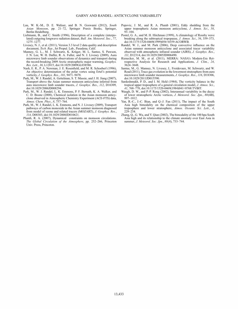
[39] The PV tendency budget (Figure A1b) shows thatthe diabatic and divergence terms are positive, of simi-lar size and well correlated in the model, and these twoterms lead to increases in low PV area linked to enhancedconvection. The actual area changes (tendency term) aresmall compared to the forcing terms, and the forcing is bal-anced by a strong negative term, calculated here as residual(Figure A1b, green line). The residual represents the mix-ing term in equation (3), which by definition cannot becalculated explicitly as it involves subscale mixing. Equat-ing the calculated residual to (unresolved) damping or PVmixing, we interpret the balance in Figure A1 as follows.

Figure A1. Budget of 0.3 PV area for one season fromWACCM. (top) Area of PV = 0.3 PVU (black) and forcingterm (blue, divergence + diabatic term). (bottom) PV areatendency (black) with divergence term (blue), diabatic term(red), sum of diabatic and divergence terms (dashed black),and residual (green).

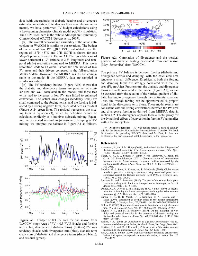
Figure A2. Correlation of divergence and the verticalgradient of diabatic heating calculated from one season(May–September) from WACCM.

The primary PV balance is between forcing (diabatic anddivergence terms) and damping, with the calculated areatendency a small difference. Empirically, both the forcingand damping terms are strongly correlated with the PVarea (Figure A1a). Furthermore, the diabatic and divergenceterms are well correlated in the model (Figure A2), as canbe expected from the relation of the vertical gradient of dia-batic heating to divergence through the continuity equation.Thus, the overall forcing can be approximated as propor-tional to the divergence term alone. These model results areconsistent with the strong correlations between the PV areaand divergence forcing as derived from MERRA data insection 4.2. The divergence appears to be a useful proxy forthe dynamical effects of convection in forcing PV anomalieswithin the anticyclone.

[40] Acknowledgments. HG was funded under a postdoc scholar-ship by the Deutsche Akademische Austauschdienst (DAAD). We thankD. Kinnison for providing WACCM data, and M. Park, L. Pan, andC. Homeyer for discussion and helpful comments on the manuscript.

ReferencesAnnamalai, H., and J. M. Slingo (2001), Active/break cycles: Diagnosis of

the intraseasonal variability of the Asian summer monsoon, Clim. Dyn.,18, 85–102, doi:10.1007/s003820100161.

Baker, A. K., T. J. Schuck, F. Slemr, P. van Velthoven, A. Zahn, andC. A. M. Brenninkmeijer (2011), Characterization of non-methanehydrocarbons in Asian summer monsoon outflow observed by thecaribic aircraft, Atmos. Chem. Phys., 11, 503–518, doi:10.5194/acp-11-503-2011.

Bodeker, G., J. Scott, K. Kreher, and R. McKenzie (2001), Global ozonetrends in potential vorticity coordinates using toms and gome inter-compared against the Dobson network: 1978–1998, J. Geophys. Res.,106(D19), 23,029–23,042.

Butchart, N., and E. Remsberg (1986), The area of the stratospheric polarvortex as a diagnostic for tracer transport on an isentropic surface, J.Atmos. Sci., 43(13), 1319–1339.

Dethof, A., A. O’Neill, J. M. Slingo, and H. G. J. Smit (1999), A mecha-nism for moistening the lower stratosphere involving the Asian summermonsoon, Q. J. R. Meteorol. Soc., 125, 1079–1106.

Garcia, R. R., D. R. Marsh, D. E. Kinnison, B. A. Boville, and F.Sassi (2007), Simulation of secular trends in the middle atmosphere,1950–2003, J. Geophys. Res., 112, D09301, doi:10.1029/2006JD007485.

Gill, A. E. (1980), Some simple solutions for heat-induced tropical circula-tion, Q. J. R. Meteorol. Soc., 106, 447–462, doi:10.1256/smsqj.44904.

Haynes, P. H., and M. E. McIntyre (1987), On the evolution of vor-ticity and potential vorticity in the presence of diabatic heating andfrictional or other forces, J. Atmos. Sci., 44, 828–841, doi:10.1175/1520-0469(1987)044.

Holton, J. R. (2004), An Introduction to Dynamic Meteorology, 4th ed.,International Geophysics Series, Academic Press, San Diego, New York.

Hoskins, B. J., and M. J. Rodwell (1995), A model of the Asian summermonsoon, I: The global scale, J. Atmos. Sci., 52, 1329–1340.

Hsu, C., and R. Plumb (2000), Non-axisymmetric thermally driven circu-lations and upper tropospheric monsoon dynamics, J. Atmos. Sci., 57,1254–1276.

13,432


Lau, W. K.-M., D. E. Waliser, and B. N. Goswami (2012), SouthAsian Monsoon, pp. 21–72, Springer Praxis Books, Springer,Berlin Heidelberg.

Liebmann, B., and C. Smith (1996), Description of a complete (interpo-lated) outgoing longwave radiation dataset, Bull. Am. Meteorol. Soc., 77,1275–1277.

Livesey, N. J., et al. (2011), Version 3.3 level 2 data quality and descriptiondocument, Tech. Rep., Jet Propul. Lab., Pasadena, Calif.

Manney, G. L., M. J. Schwartz, K. Krüger, M. L. Santee, S. Pawson,J. N. Lee, W. H. Daffer, R. A. Fuller, and N. J. Livesey (2009), Auramicrowave limb sounder observations of dynamics and transport duringthe record-breaking 2009 Arctic stratospheric major warming, Geophys.Res. Lett., 36, L12815, doi:10.1029/2009GL038586.

Nash, E. R., P. A. Newman, J. E. Rosenfield, and M. R. Schoeberl (1996),An objective determination of the polar vortex using Ertel’s potentialvorticity, J. Geophys. Res., 101, 9471–9478.

Park, M., W. J. Randel, A. Gettelman, S. T. Massie, and J. H. Jiang (2007),Transport above the Asian summer monsoon anticyclone inferred fromaura microwave limb sounder tracers, J. Geophys. Res., 112, D16309,doi:10.1029/2006JD008294.

Park, M., W. J. Randel, L. K. Emmons, P. F. Bernath, K. A. Walker, andC. D. Boone (2008), Chemical isolation in the Asian monsoon anticy-clone observed in Atmospheric Chemistry Experiment (ACE-FTS) data,Atmos. Chem. Phys., 8, 757–764.

Park, M., W. J. Randel, L. K. Emmons, and N. J. Livesey (2009), Transportpathways of carbon monoxide in the Asian summer monsoon diagnosedfrom model of ozone and related tracers (MOZART), J. Geophys. Res.,114, D08303, doi:10.1029/2008JD010621.

Plumb, R. A. (2007), Dynamical constraints on monsoon circulations.The Global Circulation of the Atmosphere, pp. 252–266, PrincetonUniv. Press, Princeton.

Popovic, J. M., and R. A. Plumb (2001), Eddy shedding from theupper tropospheric Asian monsoon anticyclone, J. Atmos. Sci., 58,93–104.

Postel, G. A., and M. H. Hitchman (1999), A climatology of Rossby wavebreaking along the subtropical tropopause, J. Atmos. Sci., 56, 359–373,doi:10.1175/1520-0469(1999)056<0359:ACORWB.

Randel, W. J., and M. Park (2006), Deep convective influence on theAsian summer monsoon anticyclone and associated tracer variabilityobserved with atmospheric infrared sounder (AIRS), J. Geophys. Res.,111, D12314, doi:10.1029/2005JD006490.

Rienecker, M. M., et al. (2011), MERRA: NASA’s Modern-Era Ret-rospective Analysis for Research and Applications, J. Clim., 24,3624–3648.

Santee, M., G. Manney, N. Livesey, L. Froidevaux, M. Schwartz, and W.Read (2011), Trace gas evolution in the lowermost stratosphere from auramicrowave limb sounder measurements, J. Geophys. Res., 116, D18306,doi:10.1029/2011JD015590.

Sardeshmukh, P. D., and I. M. Held (1984), The vorticity balance in thetropical upper troposphere of a general circulation model, J. Atmos. Sci.,41, 768–778, doi:10.1175/1520-0469(1984)041<0768:TVBIT.

Waugh, D. W., and P.-P. Rong (2002), Interannual variability in the decayof lower stratospheric Arctic vortices, J. Meteorol. Soc. Jpn., 80(4B),997–1012.

Yan, R.-C., J.-C. Bian, and Q.-J. Fan (2011), The impact of the SouthAsia high bimodality on the chemical composition of the uppertroposphere and lower stratosphere, Atmos. Oceanic Sci. Lett., 4,229–234.

Zhang, Q., G. Wu, and Y. Qian (2002), The bimodality of the 100 hpa SouthAsia high and its relationship to the climate anomaly over East Asia insummer, J. Meteorol. Soc. Jpn., 80(4), 733–744.

13,433

Documents

Dynamic variability of the Asian monsoon anticyclone ... and Randel 2013.pdfGARNY AND RANDEL: ANTICYCLONE VARIABILITY Figure 3. (a) PV at 360K and at 90ıE as a function of latitude