Dynamics of Inflationary Universes with Positive Spatial Curvature

P1: GCR

General Relativity and Gravitation (GERG) pp549-gerg-377308 August 21, 2002 18:31 Style file version May 27, 2002

General Relativity and Gravitation, Vol. 34, No. 9, September 2002 (C© 2002)

Dynamics of Inflationary Universes with PositiveSpatial Curvature

G. F. R. Ellis,1,2 W. Stoeger,3 P. McEwan,1 and P. Dunsby1,4

Received February 19, 2002

If the spatial curvature of the universe is positive, then the curvature term will alwaysdominate at early enough times in a slow-rolling inflationary epoch. This enhancesinflationary effects and hence puts limits on the possible number of e-foldings that canhave occurred, independently of what happened before inflation began and in particularwithout regard for what may have happened in the Planck era. We use a simple multi-stage model to examine this limit as a function of the present density parameterÄ0 andthe epoch when inflation ends.

KEY WORDS: Inflationary Universe; closed model.

1. POSITIVELY-CURVED INFLATIONARY MODELS?

The inflationary universe paradigm [1] is the premiere causative conceptin present-day physical cosmology, and faith in this view has been bolstered bythe recent measurements of a second and third peak in the cosmic blackbodybackground radiation (CBR) anisotropy spectrum [2], as has been predicted onthe basis of inflationary scenarios. The best-fit models vary according to the priorassumptions made when analyzing the data [3], but together with supernova data [4]suggest a model (Ä30 ≈ 0.7, Äm0 ≈ 0.3, Ä0 ≈ 1) with a non-zero cosmologicalconstant and sufficient matter to make it almost flat, implying the universe iscosmological-constant dominated from the present back to a redshift of about

1Department of Applied Mathematics, University of Cape Town, Rondebosch 7700, Cape Town, SouthAfrica.

2Erwin Schrodinger Institute, Vienna, Austria.3Vatican Observatory, Tucson, Arizona, USA.4e-mail: [email protected]

1445

0001-7701/02/0900-1445/0C© 2002 Plenum Publishing Corporation

P1: GCR


1446 Ellis, Stoeger, McEwan, and Dunsby

z= 0.326, and matter dominated back from then to decoupling. While the set ofmodels compatible with the data include those with flat spatial sections (k = 0),i.e. a critical effective energy density:Ä0 = 1, they also include positive spatialcurvature (k = +1 :Ä0 > 1) models and negative curvature (k = −1 :Ä0 < 1)ones, with a weak implication that the best-fit models have positive curvature [3].This has important implications: if true, it means that the best-fit universe models,extrapolated unchanged beyond the visual horizon, have finite spatial sections andcontain a finite amount of matter. Whether they will expand forever or not dependson whether the cosmological constant is indeed constant (when these models willexpand forever even thoughk = +1), or varies with time and decays away in thefar future (when they will recollapse).

It should be noted that while inflation is taken to predict that the universe isvery close to flat at the present time, it doesnot imply that the spatial sections areexactlyflat; indeed that case is infinitely improbable, and neither inflation nor anyother known physical process is able to specify that curvature, nor dynamicallychange it from its initial value [5]. Thus there is no reason to believe on the basis ofinflationary dynamics thatk = 0. Indeed positive-curvature universes have beenclaimed to have major philosophical advantages over the flat and negatively curvedcases, being introduced first by Einstein [7] in an attempt to solve the problem ofboundary conditions at infinity, and then adopted as the major initial paradigm incosmology by Friedmann, Lemaitre, and Eddington. This view was then taken up,in particular by Wheeler [8], to the extent that the famous book on gravitation heco-authored with Thorne and Misner [9] almost exclusively considered the positivecurvature case, labeling the negatively curved case ‘model universes that violateEinstein’s conception of cosmology’ (see page 742). Without going that far, it iscertainly worth exploring the properties of inflationary models withk = +1 [6],particularly as this case has been marginally indicated by some recent observations.

In this paper we examine the dynamics of inflationary universe models (i) withpositive curvature, and (ii) where a cosmological constant approximation holds inthe inflationary era, deriving new limits on the allowed numbers of e-foldings ofsuch models as a function of the epoch when inflation ended and of the present-day total energy density parameterÄ0. These limits do not contradict standardinflationary understanding. Indeed, in a sense they enhance inflation, since earlyin the inflationary epochs ofk = +1 universes, the deceleration parameter ismorenegative than in thek = 0 models. We only model the Hot Big Bang era (postinflation to the present day) and the Inflationary era; our results are independent ofthe dynamics before inflation starts. Similar results will hold for all models withonly slow rolling inflation. Although the observational evidence is that there iscurrently a non-zero cosmological constant, as mentioned above, for simplicity wewill consider here only the case of an almost-flatk = +1 universe with vanishingcosmological constant after the end of inflation. This approximation will not affectthe statements derived concerning dynamics up to the time of decoupling, but will

P1: GCR


Dynamics of Inflationary Universes with Positive Spatial Curvature 1447

make a small difference to estimates of the number of e-foldings given here. Wewill give more accurate estimates in a more detailed paper on these dynamics [10].An accompanying paper discusses the implications of this dynamical behaviourfor horizons in positively-curved inflationary universes [11].

2. BASIC EQUATIONS

The positive-curvature Friedmann-Lemaitre (FL) cosmological model instandard form has a scale factorS(t) normalized so that the spatial metric has unitspatial curvature at the timet∗ whenS(t∗) = 1 (see e.g. [14], [15]). The spatial sec-tions are closed atr− coordinate value increment 2π ; that is,P = (t, r − π, θ, φ)and P′ = (t, r + π, θ, φ) are necessarily the same point, for arbitrary values oft, r, θ, φ, and wherever the origin of coordinates is chosen. The Hubble Parameteris H (t) = S(t)/S(t), with present valueH0 = 100h km/sec/Mpc. The dimen-sionless quantityh probably lies in the range 0.7< h < 0.5.

2.1. k = +1 Dynamics

The dynamic behaviour is determined by the Friedmann equation fork = +1FL universes: (

H (t)

c

)2

= κµ(t)+33

− 1

S(t)2, (1)

whereκ is the gravitational constant in appropriate units and3 the cosmologicalconstant (see e.g. [14], [15]). The way this works out in practice is determined bythe matter content of the universe, whose total energy densityµ(t) and pressurep(t) necessarily obey the conservation equation

µ(t)+ (µ(t)+ p(t)/c2) 3H (t) = 0. (2)

The nature of the matter is determined by the equation of state relatingp(t) andµ(t); we will describe this in terms of a parameterγ (t) defined by

p(t)/c2 = (γ (t)− 1)µ(t), γ ∈ [0, 2]. (3)

During major epochs of the universe’s history, the matter behaviour is well-described by this relation withγ a constant (but with that constant different atvarious distinct dynamical epochs). In particular,γ = 1 represents pressure freematter (baryonic matter),γ = 4

3 represents radiation (or relativistic matter), andγ = 0 gives an effective cosmological constant of magnitude3 = κµ (by equa-tion (2),µ will then be unchanging in time). In general,µ will be a sum of suchcomponents. However we can to a good approximation represent the universe asa series of simple epochs with only one or at most two components in each epoch.

P1: GCR



The dimensionless density parameterÄi (t) for any matter componenti isdefined by

Äi (t) ≡ κµi (t)

3

(c

H (t)

)2

⇒ Äi 0 = κµi 0c2

3H20

(4)

whereÄi 0 represents the value ofÄi (t) at some arbitrary reference timet0, oftentaken to be the present time. One can define such a density parameter for eachenergy density present. We can represent a cosmological constant in terms of anequivalent energy densityκµ3 = 3; from now on we omit explicit reference to3, assuming it will be included in this way when necessary. From the Friedmannequation (1), the scale factorS(t) is related to the total density parameterÄ(t),defined by

Ä(t) =∑

i

Äi (t) = κµ(t)

3

(c

H (t)

)2

> 1, (5)

via the relation

1

S(t)2=(

H (t)

c

)2

(Ä(t)− 1)⇒(

H0

c

)2

= 1

S20 (Ä0− 1)

, Ä0 ≡ κµ0

3

c2

H20

> 1, (6)

whereÄ0 is the present total value:Ä0 =∑

i Äi 0. Whenγ is constant for somecomponent labeledi , the conservation equation (2) gives

κµi (t)

3= Äi 0

(H0

c

)2( S0

S(t)

)3γ

= 1

S20

(Äi 0

Ä0− 1

)(S0

S(t)

)3γ

(7)

for each component, on using (6). The integral

9(A, B) ≡∫ tB

tA

cdt

S(t)= c

∫ SB

SA

dS

SS(8)

is the conformal time, used in the usual conformal diagrams for FL universes[13].

2.2. Matter and Radiation Eras

During thecombined matter and radiation eras, i.e. whenever we can ig-nore the3 term in the Friedmann equation (1) but include separately conservedpressure-free matter and radiation:µ = µm + µr , each separately obeying (7), asimple analytic expression relatesS and9 [15]. For such combined matter and

P1: GCR



radiation, referred to an arbitrary reference pointP in this epoch, we have the exactsolution

S(9)P = SP

(1

2

ÄmP

ÄP − 1(1− cos9)+

√Är P

ÄP − 1sin9

), (9)

where the first term is due to the matter and the second is due to radiation. It isremarkable that they are linearly independent in this non-linear solution. We obtainthe pure radiation solution ifÄmp = 0, and the pure matter solution ifÄr p = 0.The origin of the time9 has been chosen so that an initial singularity occurs at9 = 0, if the Hot Big Bang era in this model is extended as far as possible (withoutan inflationary epoch). We will use this representation from the end of inflationto the present day. It will be accurate whenever the matter and radiation are non-interacting in the sense that their energy densities are separately conserved, butinaccurate when they are strongly interacting, for example when pair productiontakes place.

2.3. Cosmological Constant Epoch

During acosmological constant-dominated era, i.e. when3 > 0 and we canignore matter and radiation in (1), we can find thegeneral solution(with a suitablychosen origin of time) in the simple collapsing and re-expanding form

S(t) = S(0) coshλt, λ ≡ c

√3

3, S(0)≡ c

λ, (10)

where t = 0 corresponds to the minimum of the radius function, i.e. the turn-around from infinite collapse to infinite expansion, and soS(0) is the minimumvalue ofS(t) (note that we can have independent time scales in the different eraswith different zero-points, provided we match properly between eras as discussednext). This is of course just the de Sitter universe represented as a Robertson-Walkerspacetime with positively-curved space sections [18], and can be used to representan inflationary universe era for models withk = +1 if we restrict ourselves to theexpanding epoch

t ≥ ti ≥ 0 (11)

for some suitable initial timeti which occurs after the end of the Planck era, soti ≥ tPlanck. We will represent the inflationary era (preceding the Hot Big Bangera) in this way.

The Hubble parameter isH (t) = λ tanhλt (zero att = 0 and positive fort > 0) and the density parameterÄ3(t) is given by

Ä3(t) = 3

3

c2

H2(t)= 1

(tanhλt)2, (12)

P1: GCR



which diverges ast → 0 and tends to 1 ast →∞. The inflationary effect isenhanced in such models as compared withk = 0 models, because the decelerationparameterq = −S/(SH2) is here even more negative than in those scale-freemodels.

2.4. Joining Different Eras

Junction conditions required in joining two eras with different equations ofstate are that we must haveS(t) andS(t) continuous there, thusH (t) is continuousalso. By the Friedmann equation this implies in turn thatµ(t) is continuous, soby its definitionÄ(t) is also continuous (note that it isp(t) that is discontinuouson spacelike surfaces of discontinuity). We need to demand, then, that any two ofthese quantities are continuous where the equation of state is discontinuous; forour purposes it will be convenient to take them asS(t) andÄ(t). Thus we need toknow S(t) andÄ(t) at the beginning and end of each era to get a matching withS− = S+ andÄ− = Ä+.

The matching we need to perform is between the Hot Big Bang era and theInflationary era. Now for combined matter and radiation, referred to an arbitraryreference pointP, we have (9). Writing the same solution in the same form (withthe initial singularity at9 = 0 in both cases) but referred to another reference pointQ, we have the same expressions but withP replaced byQ everywhere. As theseare the same evolutions referred to different events,S(9)P = S(9)Q for all9, sothey must have identical functional forms. Matching the two expressions for all9,

the coefficients for cos9 and sin9 on each side must separately be equal. LettingSP/SQ = R, this gives the total density parameterÄQ(R) = ÄmQ(R)+Är Q(R)at the eventQ in terms of the density parameter values atP. Taking the eventQto be the end of inflation and the eventP to be here and now given byt = t0, wefind

ÄQ(R) = R (Äm0+ RÄr 0)

R2Är 0+ RÄm0− (Äm0+Är 0− 1). (13)

The matching condition is then given by assumingÄ3(tQ) = ÄQ(R). We areassuming here that the details of reheating at the end of inflation are irrelevant:conservation of total energy must result in the total value ofÄ at Q being constantduring any such change (one can easily modify this condition if desired). This givesÄ3(tQ) at the end of inflationQ by (12), which then givestQ in the inflationaryepoch described by (10):

tQ = 1

λarctanh

1√Ä3(tQ)

= 1

λarctanh

1√ÄQ(R)

, (14)

with ÄQ(R) given by (13). Note that in these expressions, the ratioR =S0/SQ isthe expansion ratio from the end of inflation until today.

P1: GCR



3. PARAMETER LIMITS

3.1. Maximum Number of e-Foldings:Nmax

The maximum number of e-foldings available until timetQ with the givenvalueÄ3(tQ) is given by the expansion form (10) witht = tQ given by (14):

eNmax = S(tQ)

S(0)= cosh

(arctanh

1√ÄQ(R)

), (15)

becauseS(0) is the minimum value ofS(t) (by our choice of time coordinate forthis era, the throat where expansion starts is set att = 0) andt is restricted by (11).If the universe starts off at any time later thant = 0 in the expanding erat > 0,there will be fewer e-foldings before the end of inflationtQ.

Defining the difference ofÄ0 from unity to beδ > 0:

Ä0 = 1+ δ ⇔ Äm0 = 1+ δ −Är 0, (16)

we find from (15) and (13) that the maximum number of inflationary e-foldingsthat can occur before inflation ends at an eventQ with expansion rationR, is

Nmax(R, δ) = ln

[cosh

(arctanh

√α − δ√α

)]= 1

2lnα − 1

2ln δ, (17)

where

α ≡ R2Är 0+ R( 1+ δ −Är 0).

This e-folding limit essentially represents a matching of the present day radiationdensityÄr 0 to the energy density limits that may be imposed at the end of inflation,which will place restrictions on the possible value of the expansion ratioR. It doesnot take into account matter-radiation conversions in the Hot Big Bang era, whichwe consider in a later section.

3.2. Density Parameter Variation from Unity: δ

What are the implications? The inversion of (17) in terms ofδ is

δ(R, Nmax) = RRÄr 0+ 1−Är 0

e2Nmax −R . (18)

Note that this value diverges whenNmax= 12 ln(R), so this is the value correspond-

ing to a turn-around today (Ä0 = ∞⇔ H0 = 0). Thus there is a smallest valuefor Nmax for each set of parametersÄr 0,R.

P1: GCR



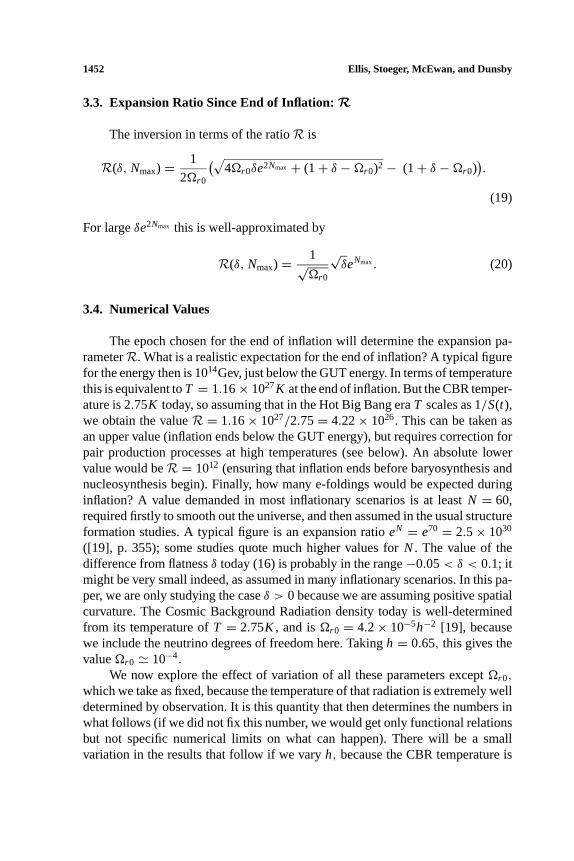
3.3. Expansion Ratio Since End of Inflation:R

The inversion in terms of the ratioR is

R(δ, Nmax) = 1

2Är 0

(√4Är 0δe2Nmax + (1+ δ −Är 0)2− (1+ δ −Är 0)

).

(19)

For largeδe2Nmax this is well-approximated by

R(δ, Nmax) = 1√Är 0

√δeNmax. (20)

3.4. Numerical Values

The epoch chosen for the end of inflation will determine the expansion pa-rameterR. What is a realistic expectation for the end of inflation? A typical figurefor the energy then is 1014Gev, just below the GUT energy. In terms of temperaturethis is equivalent toT = 1.16× 1027K at the end of inflation. But the CBR temper-ature is 2.75K today, so assuming that in the Hot Big Bang eraT scales as 1/S(t),we obtain the valueR = 1.16× 1027/2.75= 4.22× 1026. This can be taken asan upper value (inflation ends below the GUT energy), but requires correction forpair production processes at high temperatures (see below). An absolute lowervalue would beR = 1012 (ensuring that inflation ends before baryosynthesis andnucleosynthesis begin). Finally, how many e-foldings would be expected duringinflation? A value demanded in most inflationary scenarios is at leastN = 60,required firstly to smooth out the universe, and then assumed in the usual structureformation studies. A typical figure is an expansion ratioeN = e70 = 2.5× 1030

([19], p. 355); some studies quote much higher values forN. The value of thedifference from flatnessδ today (16) is probably in the range−0.05< δ < 0.1; itmight be very small indeed, as assumed in many inflationary scenarios. In this pa-per, we are only studying the caseδ > 0 because we are assuming positive spatialcurvature. The Cosmic Background Radiation density today is well-determinedfrom its temperature ofT = 2.75K , and isÄr 0 = 4.2× 10−5h−2 [19], becausewe include the neutrino degrees of freedom here. Takingh = 0.65, this gives thevalueÄr 0 ' 10−4.

We now explore the effect of variation of all these parameters exceptÄr 0,

which we take as fixed, because the temperature of that radiation is extremely welldetermined by observation. It is this quantity that then determines the numbers inwhat follows (if we did not fix this number, we would get only functional relationsbut not specific numerical limits on what can happen). There will be a smallvariation in the results that follow if we varyh, because the CBR temperature is

P1: GCR



converted into an equivalentÄr 0 value by the present value of the Hubble constant(expressed in terms ofh).

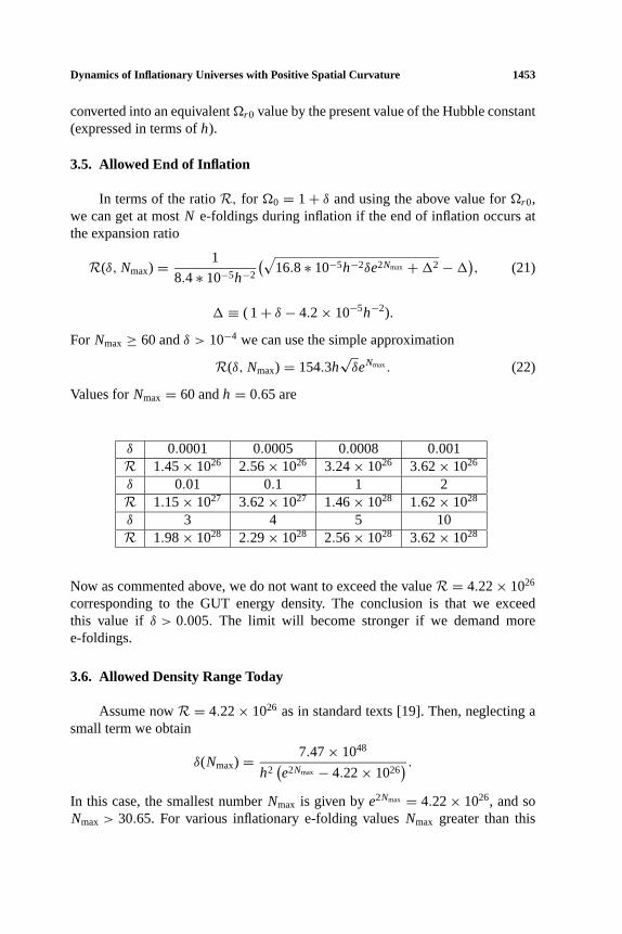
3.5. Allowed End of Inflation

In terms of the ratioR, for Ä0 = 1+ δ and using the above value forÄr 0,we can get at mostN e-foldings during inflation if the end of inflation occurs atthe expansion ratio

R(δ, Nmax) = 1

8.4 ∗ 10−5h−2

(√16.8 ∗ 10−5h−2δe2Nmax +12−1), (21)

1 ≡ ( 1+ δ − 4.2× 10−5h−2).

For Nmax≥ 60 andδ > 10−4 we can use the simple approximation

R(δ, Nmax) = 154.3h√δeNmax. (22)

Values forNmax= 60 andh = 0.65 are

δ 0.0001 0.0005 0.0008 0.001R 1.45× 1026 2.56× 1026 3.24× 1026 3.62× 1026

δ 0.01 0.1 1 2R 1.15× 1027 3.62× 1027 1.46× 1028 1.62× 1028

δ 3 4 5 10R 1.98× 1028 2.29× 1028 2.56× 1028 3.62× 1028

Now as commented above, we do not want to exceed the valueR = 4.22× 1026

corresponding to the GUT energy density. The conclusion is that we exceedthis value if δ > 0.005. The limit will become stronger if we demand moree-foldings.

3.6. Allowed Density Range Today

Assume nowR = 4.22× 1026 as in standard texts [19]. Then, neglecting asmall term we obtain

δ(Nmax) = 7.47× 1048

h2(e2Nmax − 4.22× 1026

) .In this case, the smallest numberNmax is given bye2Nmax = 4.22× 1026, and soNmax> 30.65. For various inflationary e-folding valuesNmax greater than this

P1: GCR



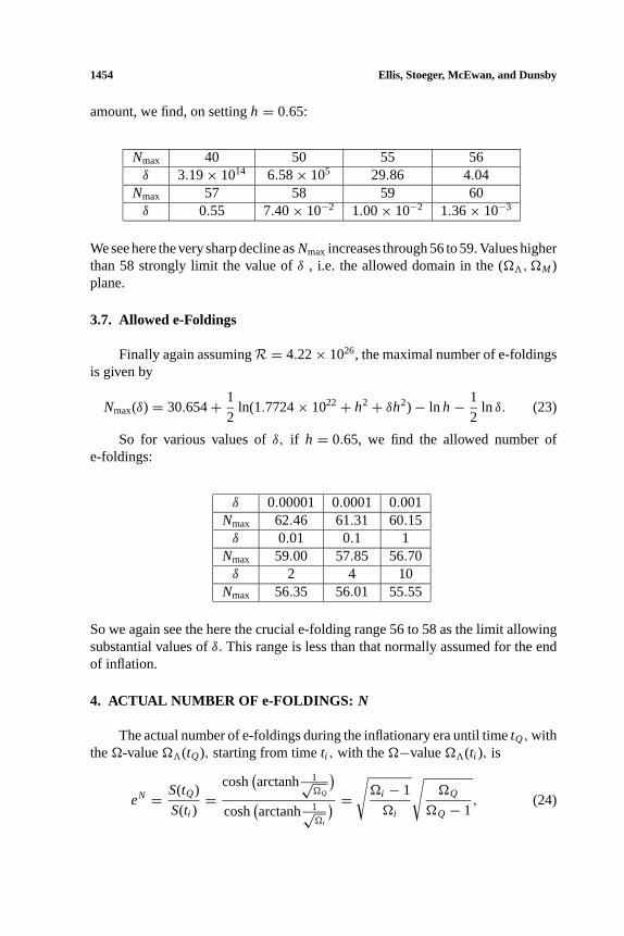
amount, we find, on settingh = 0.65:

Nmax 40 50 55 56δ 3.19× 1014 6.58× 105 29.86 4.04

Nmax 57 58 59 60δ 0.55 7.40× 10−2 1.00× 10−2 1.36× 10−3

We see here the very sharp decline asNmaxincreases through 56 to 59. Values higherthan 58 strongly limit the value ofδ , i.e. the allowed domain in the (Ä3,ÄM )plane.

3.7. Allowed e-Foldings

Finally again assumingR = 4.22× 1026, the maximal number of e-foldingsis given by

Nmax(δ) = 30.654+ 1

2ln(1.7724× 1022+ h2+ δh2)− ln h− 1

2ln δ. (23)

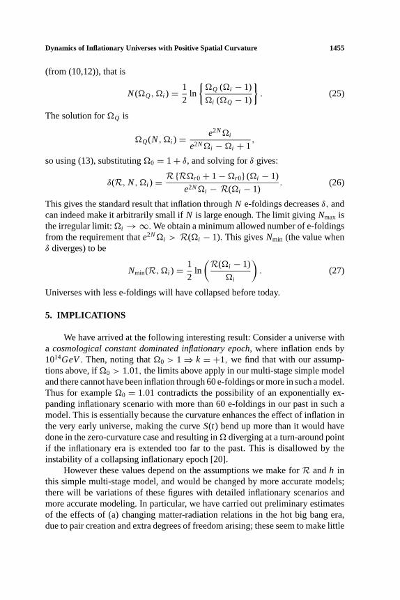
So for various values ofδ, if h = 0.65, we find the allowed number ofe-foldings:

δ 0.00001 0.0001 0.001Nmax 62.46 61.31 60.15δ 0.01 0.1 1

Nmax 59.00 57.85 56.70δ 2 4 10

Nmax 56.35 56.01 55.55

So we again see the here the crucial e-folding range 56 to 58 as the limit allowingsubstantial values ofδ. This range is less than that normally assumed for the endof inflation.

4. ACTUAL NUMBER OF e-FOLDINGS: N

The actual number of e-foldings during the inflationary era until timetQ,withtheÄ-valueÄ3(tQ), starting from timeti , with theÄ−valueÄ3(ti ), is

eN = S(tQ)

S(ti )=

cosh(arctanh 1√

ÄQ

)cosh

(arctanh 1√

Äi

) = √Äi − 1

Äi

√ÄQ

ÄQ − 1, (24)

P1: GCR



(from (10,12)), that is

N(ÄQ, Äi ) = 1

2ln

{ÄQ (Äi − 1)

Äi (ÄQ − 1)

}. (25)

The solution forÄQ is

ÄQ(N, Äi ) = e2NÄi

e2NÄi −Äi + 1,

so using (13), substitutingÄ0 = 1+ δ, and solving forδ gives:

δ(R, N, Äi ) = R {RÄr 0+ 1−Är 0} (Äi − 1)

e2NÄi − R(Äi − 1). (26)

This gives the standard result that inflation throughN e-foldings decreasesδ, andcan indeed make it arbitrarily small ifN is large enough. The limit givingNmax isthe irregular limit:Äi →∞.We obtain a minimum allowed number of e-foldingsfrom the requirement thate2NÄi > R(Äi − 1). This givesNmin (the value whenδ diverges) to be

Nmin(R, Äi ) = 1

2ln

(R(Äi − 1)

Äi

). (27)

Universes with less e-foldings will have collapsed before today.

5. IMPLICATIONS

We have arrived at the following interesting result: Consider a universe witha cosmological constant dominated inflationary epoch, where inflation ends by1014GeV. Then, noting thatÄ0 > 1⇒ k = +1, we find that with our assump-tions above, ifÄ0 > 1.01, the limits above apply in our multi-stage simple modeland there cannot have been inflation through 60 e-foldings or more in such a model.Thus for exampleÄ0 = 1.01 contradicts the possibility of an exponentially ex-panding inflationary scenario with more than 60 e-foldings in our past in such amodel. This is essentially because the curvature enhances the effect of inflation inthe very early universe, making the curveS(t) bend up more than it would havedone in the zero-curvature case and resulting inÄ diverging at a turn-around pointif the inflationary era is extended too far to the past. This is disallowed by theinstability of a collapsing inflationary epoch [20].

However these values depend on the assumptions we make forR andh inthis simple multi-stage model, and would be changed by more accurate models;there will be variations of these figures with detailed inflationary scenarios andmore accurate modeling. In particular, we have carried out preliminary estimatesof the effects of (a) changing matter-radiation relations in the hot big bang era,due to pair creation and extra degrees of freedom arising; these seem to make little

P1: GCR



difference; and (b) the effect of a previous radiation dominated era at the start ofinflation, resulting in an initial inflationary era where radiation was non-negligible.The basic effect would remain in this case, but the numbers estimated above wouldchange. These refinements will be considered in a paper [10] examining the relevantdynamics in more detail.

The main point of this paper is that such limits exist and should be takeninto account when examining inflationary models withk = +1. The limits givenabove are only for the simple model considered here; they will be different in moredetailed models.

5.1. Criterion for This to Happen

This calculation is for an epoch of inflation driven by a cosmological con-stant. However there are numerous other forms of inflation. The key point thenis that similar effects will occur in all inflationary models in which the effectiveenergy density of the scalar field varies more slowly than the curvature term in theFriedmann equation, which varies asS−2. From (7), this will happen if 3γ < 2.The limiting behaviour where the energy density mimics the curvature term isa coasting universe with 3γ = 2⇔ µ+ 3p/c2 = 0. Scalar fields can give anyeffectiveγ from 0 to 2, so there will be fast-rolling scalar-field driven modelswhere 3γ > 2. However these will not then be inflationary, for they will not be ac-celerating (the requirement for an accelerating universe isµ+ 3p/c2 < 0). Thuseffects of the kind considered here will occur in all positive curvature inflationaryuniverses, but power-law models will have different detailed behaviour than theones with an effective cosmological constant calculated above. The numbers willbe different and the constraints may be much less severe.

6. CONCLUSION

If we everobservationally determinethatÄ0 > 1⇒ k = +1, thenδ > δ0

whereδ0 is some value sufficiently large that we can distinguish the value ofÄ0

from unity, and so will certainly be greater than 0.01 (for otherwise we couldnot observationally prove thatÄ0 > 1). Thus there cannot in this case have beenexponential inflation through some value that will depend on the model used; in thecase considered above, it is about 59 e-foldings, so such an inflationary scenario,with 60 or more e-foldings, could not have occurred. Hence it is of considerableinterest to try all forms of cosmological tests to determine ifÄ0 > 1. It is of coursepossible we will never determine observationally whetherÄ0 > 1 orÄ0 < 1. Thepoint of this paper is to comment that there are substantial dynamical implicationsif we can ever make this distinction on the basis of observational data. There isnot a corresponding implication on the negative side, i.e. forδ < 0⇔ Ä0 < 1(one might then claim limits on the number of e-foldings caused by limits on

P1: GCR



ÄPlanck or HPlanck at the end of the Planck time; but the results presented here areindependent of any such considerations). Thus if we could ever determine say thatÄ0 = 0.99, this would not imply any limit on the number of e-foldings, whereasfor Ä0 = 1.01, such restrictions are implied.

Many inflationary theorists would not find this conclusion surprising, as theywould expect the final value ofδ to be very small, as is indicated here, and wouldassume that if we were too far from flat today this was just because, given thestarting conditions for the inflationary era, one had not had enough e-foldings totruly flatten the universe; so more e-foldings should be employed, and we wouldend up much closer to flat today. However they have arrived at that conclusionby examining the case of scale-free (exponential) expansion, which arises whenthe spatial curvature term in the Friedmann equation is ignored, and then placingbounds on the value of the allowed energy density at the start of inflation. But thepoint of the present analysis is precisely that one cannot ignore that curvature termat early enough times in an inflationary epoch driven by a cosmological constant.It is the resulting non-scale-free behaviour that leads to the restrictions on allowede-foldings calculated above, irrespective of the initial conditions inherited from thePlanck era. The implication is that if you call up the extra e-foldings needed forthat programme just outlined, and end up consistent with the presently observedCBR density, then necessarily a limit such asÄ0 < 1.001 holds. Thus this kindof result strengthens the inflationary intuition. However that e-folding limit is notincorporated in the models usually used to calculate the CBR anisotropy.

Indeed ifÄ0 > 1, so that only restricted e-foldings can occur and be com-patible with the observed CBR temperature, this could have significant effectson structure formation scenarios. The usual analyses resulting in the famous ob-servational planes with axesÄm andÄ3 [3] are based on assuming that morethan 60 e-foldings can occur even ifk = +1. We suggest the theoretical resultsneed re-examination in the domain wherek = +1 and only a restricted number ofe-foldings can occur. The major point is that the dynamical behaviour is discon-tinuous in that plane: asÄ0 varies from 1− δ to 1+ δ, however smallδ is, thecurvature signk changes from−1 to+1 and the corresponding termk/S(t)2 inthe Friedmann equation—which necessarily dominates over any constant term inthat equation, for smallS(t)—completely changes in its effects. Whenk = +1 iteventually causes a turn-around for somet0; whenk = −1 it hastens the onset ofthe initial singularity.

It should be noted that this conclusion is based purely on examining inflationin FL universe models with a constant vacuum energy, and is not based on examina-tions of pre-inflationary or Trans-Planckian physics on the one hand, nor on studiesof embedding such a FL region in a larger region on the other. It is based solely onthe dynamics during the inflationary epoch. However it considers only a constantvacuum energy, equivalent to a no-rolling situation, and so does not take scalarfield dynamics properly into account. It will be worth examining slow-rolling and

P1: GCR



fast-rolling models to see what the bounds of behaviour fork = +1 inflationarymodels are in those cases. We indicated above that insofar as these universes areinflationary (i.e. they are accelerating during the scalar-field dominated era), simi-lar e-folding bounds may be expected in these cases also. Also as indicated above,the results will be modified if there is a substantial radiation density during theinitial phase of inflation. We are currently investigating the difference that this willmake.

We are fully aware that in order to properly study the issue, we need to examineanisotropic and inhomogeneous geometries rather than just FL models, becauseanalyses based on FL models with their Robertson-Walker geometry cannot be usedto analyse very anisotropic or inhomogeneous eras. Nevertheless this study showsthere are major dynamical differences in inflationary FL universes withk = +1 ork = 0. The implication is (a) that we need to try all observational methods availableto determine ifk = +1, because this makes a significant difference not only to thespatial topology, but also to the dynamical and causal structure of the universe,and (b) we should examine inhomogeneous inflationary cosmological models tosee if any similar difference exists between models that are necessarily spatiallycompact, and the rest.

ACKNOWLEDGEMENT

We thank Roy Maartens, Bruce Bassett, and Claes Uggla for useful comments,and the NRF (South Africa) for financial support.

REFERENCES

[1] Guth, A. H. (1981),Phys. Rev.D23, 347. Linde, A. D. (1990),Particle Physics and InflationaryCosmology(Harwood, Chur). Kolb, E. W. and Turner, M. S. (1990),The Early Universe(Wiley,New York, 1990). For recent reviews, see Brandenberger, R. (2001):hep-th/0101119and Guth,A. H.(2001):astro-ph/0101507.

[2] Netterfield et al. (2001):astro-ph/0104460.[3] de Bernadis, P. et al:astro-ph/0011469.Bond, J. R. et al:astro-ph/0011378.Stompor, R., et al

(2001): astro-ph/015062. Wang, X. et al (2001):astro-ph/0105091. Douspis, M. et al (2001):astro-ph/0105129. de Bernadis, P. et al. (2001):astro-ph/0105296.

[4] Riess et al. (1998):Astron. Journ.116, 1009. Perlmutter et al (1999):Astrophys. Journ.517, 565.[5] Ellis, G. F. R. (1987).Astrophysical. Journal.314, 1.[6] White, M., and Scott, D. (1996).Astrophys. Journ.459, 415.[7] Einstein, A. (1917).Preuss. Akad. Wiss. Berlin., Sitzber.142; reprinted in Lorentz, H. et al.The

Principle of Relativity(Dover, New York).[8] Wheeler, J. A. (1968).Einstein’s Vision (Springer, Berlin).[9] Misner, C. W., Thorne, K. S., and Wheeler, J. A. (1973).Gravitation. (W. H. Freeman, San

Francisco).[10] G. F. R. Ellis, P. McEwan, W. Stoeger, and P. Dunsby. ‘Inflationary universe models with positive

curvature: dynamics and causality’. In preparation.

P1: GCR



[11] G. F. R. Ellis, P. McEwan, W. Stoeger, and P. Dunsby. ‘Inflationary universe models with positivecurvature: causality and horizons’. In preparation.

[12] Rindler, W. (1956).Mon. Not. Roy. Astr. Soc.116, 662.[13] Penrose, R. inRelativity Groups and Topology, Ed. C. M. DeWitt and B. S. DeWitt (Gordon and

Breach, New York, 1963). Hawking, S. W. and Ellis, G. F. R. (1973).The Large Scale Structureof Spacetime. (Cambridge University Press). Tipler, F., Clarke, C.J.S., and Ellis, G. F. R. (1980).In General Relativity and Gravitation: One Hundred Years after the Birth of Albert Einstein, Vol.2, Ed. A Held (Plenum Press, New York).

[14] Weinberg, S. (1972).Gravitation and Cosmology(Wiley, New York).[15] Ellis, G. F. R (1987), inVth Brazilian School on Cosmology and Gravitation, Ed. M. Novello

(World Scientific, Singapore).[16] Ellis, G. F. R. and Stoeger W. R., (1988).Class. Quant. Grav.5, 207.[17] G. F. R. Ellis, (1971), inGeneral Relativity and Cosmology, Proceedings of the XLVII Enrico

Fermi Summer School, Ed. R. K. Sachs (Academic Press, New York).[18] Schrodinger, E. (1956).Expanding Universes(Cambridge University Press, Cambridge).[19] Padmanabhan, T. (1993).Structure Formation in the Universe.(Cambridge University Press,

Cambridge).[20] Vilenkin, A. (1992),Phys. Rev.D46, 2355; Borde A and Vilenkin A, gr-qc/9702019.

Documents

Dynamics of Inflationary Universes with Positive Spatial Curvature