arX

iv:p

hysi

cs/0

6111

23v1

[ph

ysic

s.ao

-ph]

13

Nov

200

6 Dynamics of tsunami waves

Frederic Dias∗ Denys Dutykh∗

Abstract

The life of a tsunami is usually divided into three phases: the gen-eration (tsunami source), the propagation and the inundation. Eachphase is complex and often described separately. A brief descriptionof each phase is given. Model problems are identified. Their formula-tion is given. While some of these problems can be solved analytically,most require numerical techniques. The inundation phase is less doc-umented than the other phases. It is shown that methods based onSmoothed Particle Hydrodynamics (SPH) are particularly well-suitedfor the inundation phase. Directions for future research are outlined.

Contents

1 Introduction 2

2 Tsunami induced by near-shore earthquake 3

2.1 Introduction . . . . . . . . . . . . . . . . . . . . . . . . . . . . 32.2 Volterra’s theory of dislocations . . . . . . . . . . . . . . . . . 42.3 Dislocations in elastic half-space . . . . . . . . . . . . . . . . . 62.4 Finite rectangular source . . . . . . . . . . . . . . . . . . . . . 9

3 Propagation of tsunamis 15

3.1 Classical formulation . . . . . . . . . . . . . . . . . . . . . . . 163.2 Dimensionless formulation . . . . . . . . . . . . . . . . . . . . 173.3 Shallow-water equations . . . . . . . . . . . . . . . . . . . . . 183.4 Boussinesq equations . . . . . . . . . . . . . . . . . . . . . . . 203.5 Classical Boussinesq equations . . . . . . . . . . . . . . . . . . 213.6 Korteweg–de Vries equation . . . . . . . . . . . . . . . . . . . 22

∗Centre de Mathematiques et de Leurs Applications, Ecole Normale Superieure deCachan, 61, avenue du President Wilson, 94235 Cachan cedex, France

1 Introduction 2

4 Energy of a tsunami 23

5 Tsunami run-up 23

6 Direction for future research 26

1 Introduction

Given the broadness of the topic of tsunamis, our purpose here is torecall some of the basics of tsunami modeling and to emphasize some generalaspects, which are sometimes overlooked. The life of a tsunami is usuallydivided into three phases: the generation (tsunami source), the propagationand the inundation. The third and most difficult phase of the dynamics oftsunami waves deals with their breaking as they approach the shore. Thisphase depends greatly on the bottom bathymetry and on the coastline type.The breaking can be progressive. Then the inundation process is relativelyslow and can last for several minutes. Structural damages are mainly causedby inundation. The breaking can also be explosive and lead to the formationof a plunging jet. The impact on the coast is then very rapid. In very shallowwater, the amplitude of tsunami waves grows to such an extent that typicallyan undulation appears on the long wave, which develops into a progressivebore Chanson [2005]. This turbulent front, similar to the wave that occurswhen a dam breaks, can be quite high and travel onto the beach at greatspeed. Then the front and the turbulent current behind it move onto theshore, past buildings and vegetation until they are finally stopped by risingground. The water level can rise rapidly, typically from 0 to 3 meters in 90seconds.

The trajectory of these currents and their velocity are quite unpredictible,especially in the final stages because they are sensitive to small changes in thetopography, and to the stochastic patterns of the collapse of buildings, and tothe accumulation of debris such as trees, cars, logs, furniture. The dynamicsof this final stage of tsunami waves is somewhat similar to the dynamics offlood waves caused by dam breaking, dyke breaking or overtopping of dykes(cf. the recent tragedy of hurricane Katrina in August 2005). Hence researchon flooding events and measures to deal with them may be able to contributeto improved warning and damage reduction systems for tsunami waves in theareas of the world where these waves are likely to occur as shallow surge waves(cf. the recent tragedy of the Indian Ocean tsunami in December 2004).

Civil engineers who visited the damage area following the Boxing daytsunami came up with several basic conclusions. Buildings that had been

2 Tsunami induced by near-shore earthquake 3

constructed to satisfy modern safety standards offered a satisfactory resis-tance, in particular those with reinforced concrete beams properly integratedin the frame structure. These were able to withstand pressure associated withthe leading front of the order of 1 atmosphere (recall that an equivalent pres-sure p is obtained with a windspeed U of about 450 m/s, since p = ρairU

2/2).By contrast brick buildings collapsed and were washed away. Highly porousor open structures survived. Buildings further away from the beach survivedthe front in some cases, but they were then destroyed by the erosion of theground around the buildings by the water currents Hunt and Burgers [2005].

Section 2 provides a description of the tsunami source when the sourceis an earthquake. In Section 3, we review the equations that are often usedfor tsunami propagation. Section 4 provides a short discussion on the energyof tsunamis. Section 5 is devoted to the run-up and inundation of tsunamis.Finally directions for future research are outlined.

2 Tsunami induced by near-shore earthquake

The inversion of seismic data allows one to reconstruct the permanentdeformations of the sea bottom following earthquakes. In spite of the com-plexity of the seismic source and of the internal structure of the Earth, sci-entists have been relatively successful in using simple models for the sourceOkada [1985]. A description of Okada’s model follows.

2.1 Introduction

The fracture zones, along which the foci of earthquakes are to be found,have been described in various papers. For example, it has been suggestedthat Volterra’s theory of dislocations might be the proper tool for a quan-titative description of these fracture zones Steketee [1958]. This suggestionwas made for the following reason. If the mechanism involved in earthquakesand the fracture zones is indeed one of fracture, discontinuities in the dis-placement components across the fractured surface will exist. As dislocationtheory may be described as that part of the theory of elasticity dealing withsurfaces across which the displacement field is discontinuous, the suggestionseems reasonable.

As commonly done in mathematical physics, it is necessary for simplicity’ssake to make some assumptions. Here we neglect the curvature of the earth,its gravity, temperature, magnetism, non-homogeneity, and consider a semi-infinite medium, which is homogeneous and isotropic. We further assumethat the laws of classical linear elasticity theory hold.

2.2 Volterra’s theory of dislocations 4

Several studies showed that the effect of earth curvature is negligiblefor shallow events at distances of less than 20 Ben-Mehanem et al. [1970],Ben-Menahem et al. [1969], McGinley [1969], Smylie and Mansinha [1971].The sensitivity to earth topography, homogeneity, isotropy and half-spaceassumptions was studied and discussed recently Masterlark [2003]. The au-thor used a commercially available code, ABACUS, which is based on a finiteelement model (FEM). Six FEMs were constructed to test the sensitivity ofdeformation predictions to each assumption. The main conclusion is that thevertical layering of lateral inhomogeneity can sometimes cause considerableeffects on the deformation fields.

The usual boundary conditions for dealing with earth’s problems requirethat the surface S of the elastic medium (the earth) shall be free fromforces. The resulting mixed boundary-value problem was solved a centuryago Volterra [1907]. Later, Steketee proposed an alternative method to solvethis problem using Green’s functions Steketee [1958].

2.2 Volterra’s theory of dislocations

In order to introduce the concept of dislocation and for simplicity’s sake,this section is devoted to the case of an entire elastic space. The secondreason is that in his original paper Volterra solved the problem in this caseVolterra [1907].

Let O be the origin of a Cartesian coordinate system in an infinite elasticmedium, xi the Cartesian coordinates (i = 1, 2, 3), and ei a unit vector inthe positive xi-direction. A force F = Fek at O generates a displacementfield uk

i (P, O) at point P , which is determined by the well-known Somiglianatensor

uki (P, O) =

F

8πµ(δikr, nn − αr, ik), with α =

λ + µ

λ + 2µ. (1)

In this relation δik is the Kronecker delta, λ and µ are Lame’s constants,and r is the distance from P to O. The coefficient α can be rewritten asα = 1/2(1 − ν), where ν is Poisson’s ratio. Later we will also use Young’smodulus E, which is defined as

E =µ (3λ + 2µ)

λ + µ.

The notation r, i means ∂r/∂xi and the summation convention applies.The stresses due to the displacement field (1) are easily computed from

Hooke’s law:

σij = λδijuk,k + µ(ui,j + uj,i). (2)

2.2 Volterra’s theory of dislocations 5

We find

σkij(P, O) = −αF

4π

(

3xixjxk

r5+

µ

λ + µ

δkixj + δkjxi − δijxk

r3

)

.

The components of the force per unit area on a surface element are denotedas follows:

T ki = σk

ij · νj,

where the νj ’s are the direction cosines of the normal to the surface elementSokolnikoff and Specht [1946]. A Volterra dislocation is defined as a surfaceΣ in the elastic medium across which there is a discontinuity ∆ui in thedisplacement fields of the type

∆ui = u+i − u−

i = Ui + Ωijxj , (3)

Ωij = −Ωji. (4)

Equation (3) in which Ui and Ωij are constants is the well-known Weingartenrelation which states that the discontinuity ∆ui should be of the type of arigid body displacement, thereby maintaining continuity of the componentsof stress and strain across Σ.

The displacement field in an infinite elastic medium due to a dislocationof type (1) is then determined by Volterra’s formula Volterra [1907]

uk(y1, y2, y3) := uk(yl) =1

F

∫∫

Σ

∆uiTki dS. (5)

Once the surface Σ is given, the dislocation is essentially determined bythe six constants Ui and Ωij. Therefore we also write

uk(yl) =Ui

F

∫∫

Σ

σkij(P, Q)νjdS +

Ωij

F

∫∫

Σ

xjσkil(P, Q)−xiσ

kjl(P, Q)νldS, (6)

where Ωij takes only the values Ω12, Ω23, Ω31. Following Volterra Volterra[1907] and Love Love [1944] we call each of the six integrals in (6) an ele-mentary dislocation.

It is clear from (5) and (6) that the computation of the displacement fielduk(Q) is performed as follows: A force Fek is applied at Q, and the stressesσk

ij(P, Q) that this force generates are computed at the points P (xi) on Σ. Inparticular the components of the force on Σ are computed. After multipli-cation with prescribed weights of magnitude ∆ui these forces are integratedover Σ to give the displacement component in Q due to the dislocation onΣ.

2.3 Dislocations in elastic half-space 6

2.3 Dislocations in elastic half-space

When the case of an elastic half-space is considered, equation (5) remainsvalid, but we have to replace σk

ij by another tensor ωkij . This can be explained

by the fact that the elementary solutions for a half-space are different fromSomigliana solution (1).

The ωkij can be obtained from the displacements corresponding to nuclei

of strain in a half-space through relation (2). Steketee showed a method ofobtaining the six ωk

ij fields by using a Green’s function and derived ωk12, which

is relevant to a vertical strike-slip fault. Maruyama derived the remainingfive functions Maruyama [1964].

It is interesting to mention here that historically these solutions were firstderived in a straightforward manner by Mindlin Mindlin [1936], Mindlin and Cheng[1950], who gave explicit expressions of the displacement and stress fields forhalf-space nuclei of strain consisting of single forces with and without mo-ment. It is only necessary to write the single force results since the otherforms can be obtained by taking appropriate derivatives. Their method con-sists in finding the displacement field in Westergaard’s form of the Galerkinvector Westergaard [1935]. This vector is then determined by taking a linearcombination of some biharmonic elementary solutions. The coefficients arechosen to satisfy boundary and equilibrium conditions. These solutions werealso derived by Press in a slightly different manner Press [1965].

6x3

qx1

*x2

O

x3 = −d

δL

Wq

7

U1

U2IU3

Free surface

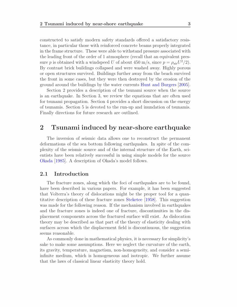
Figure 1: Coordinate system adopted in this study and geometry of thesource model

Here, we take the Cartesian coordinate system shown in Figure 1. The

2.3 Dislocations in elastic half-space 7

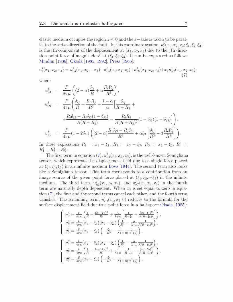
elastic medium occupies the region z ≤ 0 and the x−axis is taken to be paral-lel to the strike direction of the fault. In this coordinate system, uj

i (x1, x2, x3; ξ1, ξ2, ξ3)is the ith component of the displacement at (x1, x2, x3) due to the jth direc-tion point force of magnitude F at (ξ1, ξ2, ξ3). It can be expressed as followsMindlin [1936], Okada [1985, 1992], Press [1965]:

uji (x1, x2, x3) = uj

iA(x1, x2,−x3)−ujiA(x1, x2, x3)+uj

iB(x1, x2, x3)+x3ujiC(x1, x2, x3),

(7)where

ujiA =

F

8πµ

(

(2 − α)δij

R+ α

RiRj

R3

)

,

ujiB =

F

4πµ

(

δij

R+

RiRj

R3+

1 − α

α

[ δij

R + R3+

+Riδj3 − Rjδi3(1 − δj3)

R(R + R3)− RiRj

R(R + R3)2(1 − δi3)(1 − δj3)

]

)

,

ujiC =

F

4πµ(1 − 2δi3)

(

(2 − α)Riδj3 − Rjδi3

R3+ αξ3

[

δij

R3− 3

RiRj

R5

])

.

In these expressions R1 = x1 − ξ1, R2 = x2 − ξ2, R3 = x3 − ξ3, R2 =R2

1 + R22 + R2

3.The first term in equation (7), uj

iA(x1, x2, x3), is the well-known Somiglianatensor, which represents the displacement field due to a single force placedat (ξ1, ξ2, ξ3) in an infinite medium Love [1944]. The second term also lookslike a Somigliana tensor. This term corresponds to a contribution from animage source of the given point force placed at (ξ1, ξ2,−ξ3) in the infinitemedium. The third term, uj

iB(x1, x2, x3), and ujiC(x1, x2, x3) in the fourth

term are naturally depth dependent. When x3 is set equal to zero in equa-tion (7), the first and the second terms cancel each other, and the fourth termvanishes. The remaining term, uj

iB(x1, x2, 0) reduces to the formula for thesurface displacement field due to a point force in a half-space Okada [1985]:

u11 = F

4πµ

(

1R

+ (x1−ξ1)2

R3 + µλ+µ

[

1R−ξ3

− (x1−ξ1)2

R(R−ξ3)2

])

,

u12 = F

4πµ(x1 − ξ1)(x2 − ξ2)

(

1R3 − µ

λ+µ1

R(R−ξ3)2

)

,

u13 = F

4πµ(x1 − ξ1)

(

− ξ3R3 − µ

λ+µ1

R(R−ξ3)

)

,

u21 = F

4πµ(x1 − ξ1)(x2 − ξ2)

(

1R3 − µ

λ+µ1

R(R−ξ3)2

)

,

u22 = F

4πµ

(

1R

+ (x2−ξ2)2

R3 + µλ+µ

[

1R−ξ3

− (x2−ξ2)2

R(R−ξ3)2

])

,

u23 = F

4πµ(x2 − ξ2)

(

− ξ3R3 − µ

λ+µ1

R(R−ξ3)

)

,

2.3 Dislocations in elastic half-space 8

u31 = F

4πµ(x1 − ξ1)

(

− ξ3R3 + µ

λ+µ1

R(R−ξ3)

)

,

u32 = F

4πµ(x2 − ξ2)

(

− ξ3R3 + µ

λ+µ1

R(R−ξ3)

)

,

u33 = F

4πµ

(

1R

+ξ2

3

R3 + µλ+µ

1R

)

.

In these formulas R2 = (x1 − ξ1)2 + (x2 − ξ2)

2 + ξ23 .

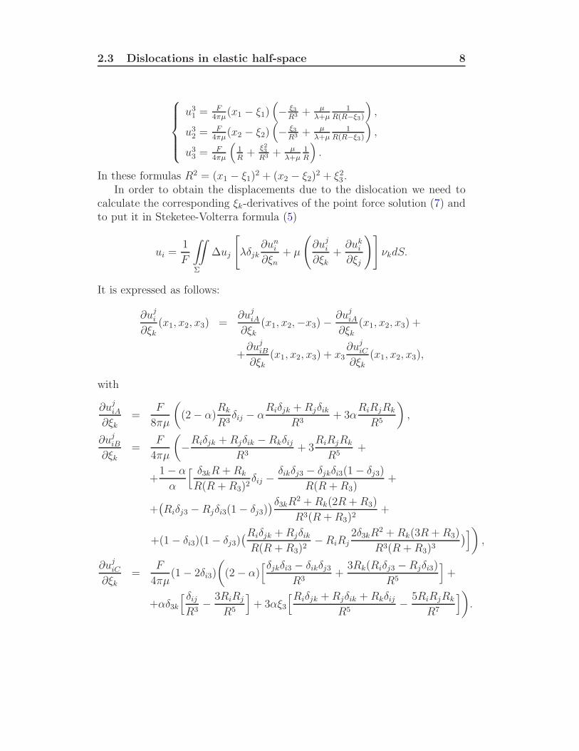
In order to obtain the displacements due to the dislocation we need tocalculate the corresponding ξk-derivatives of the point force solution (7) andto put it in Steketee-Volterra formula (5)

ui =1

F

∫∫

Σ

∆uj

[

λδjk∂un

i

∂ξn+ µ

(

∂uji

∂ξk+

∂uki

∂ξj

)]

νkdS.

It is expressed as follows:

∂uji

∂ξk

(x1, x2, x3) =∂uj

iA

∂ξk

(x1, x2,−x3) −∂uj

iA

∂ξk

(x1, x2, x3) +

+∂uj

iB

∂ξk(x1, x2, x3) + x3

∂ujiC

∂ξk(x1, x2, x3),

with

∂ujiA

∂ξk=

F

8πµ

(

(2 − α)Rk

R3δij − α

Riδjk + Rjδik

R3+ 3α

RiRjRk

R5

)

,

∂ujiB

∂ξk

=F

4πµ

(

−Riδjk + Rjδik − Rkδij

R3+ 3

RiRjRk

R5+

+1 − α

α

[ δ3kR + Rk

R(R + R3)2δij −

δikδj3 − δjkδi3(1 − δj3)

R(R + R3)+

+(

Riδj3 − Rjδi3(1 − δj3))δ3kR

2 + Rk(2R + R3)

R3(R + R3)2+

+(1 − δi3)(1 − δj3)(Riδjk + Rjδik

R(R + R3)2− RiRj

2δ3kR2 + Rk(3R + R3)

R3(R + R3)3

)

]

)

,

∂ujiC

∂ξk

=F

4πµ(1 − 2δi3)

(

(2 − α)[δjkδi3 − δikδj3

R3+

3Rk(Riδj3 − Rjδi3)

R5

]

+

+αδ3k

[ δij

R3− 3RiRj

R5

]

+ 3αξ3

[Riδjk + Rjδik + Rkδij

R5− 5RiRjRk

R7

]

)

.

2.4 Finite rectangular source 9

2.4 Finite rectangular source

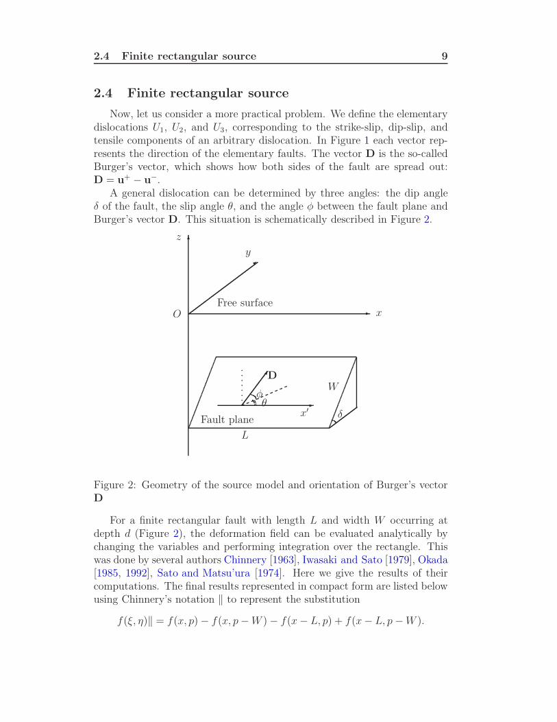
Now, let us consider a more practical problem. We define the elementarydislocations U1, U2, and U3, corresponding to the strike-slip, dip-slip, andtensile components of an arbitrary dislocation. In Figure 1 each vector rep-resents the direction of the elementary faults. The vector D is the so-calledBurger’s vector, which shows how both sides of the fault are spread out:D = u+ − u−.

A general dislocation can be determined by three angles: the dip angleδ of the fault, the slip angle θ, and the angle φ between the fault plane andBurger’s vector D. This situation is schematically described in Figure 2.

-

>

x

y6z

O

δ

7

Fault plane

Free surface

D

-x′

φθ

L

W

Figure 2: Geometry of the source model and orientation of Burger’s vectorD

For a finite rectangular fault with length L and width W occurring atdepth d (Figure 2), the deformation field can be evaluated analytically bychanging the variables and performing integration over the rectangle. Thiswas done by several authors Chinnery [1963], Iwasaki and Sato [1979], Okada[1985, 1992], Sato and Matsu’ura [1974]. Here we give the results of theircomputations. The final results represented in compact form are listed belowusing Chinnery’s notation ‖ to represent the substitution

f(ξ, η)‖ = f(x, p) − f(x, p − W ) − f(x − L, p) + f(x − L, p − W ).

2.4 Finite rectangular source 10

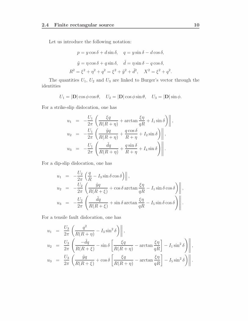
Let us introduce the following notation:

p = y cos δ + d sin δ, q = y sin δ − d cos δ,

y = η cos δ + q sin δ, d = η sin δ − q cos δ,

R2 = ξ2 + η2 + q2 = ξ2 + y2 + d2, X2 = ξ2 + q2.

The quantities U1, U2 and U3 are linked to Burger’s vector through theidentities

U1 = |D| cosφ cos θ, U2 = |D| cosφ sin θ, U3 = |D| sinφ.

For a strike-slip dislocation, one has

u1 = −U1

2π

(

ξq

R(R + η)+ arctan

ξη

qR+ I1 sin δ

)∥

∥

∥

∥

,

u2 = −U1

2π

(

yq

R(R + η)+

q cos δ

R + η+ I2 sin δ

)∥

∥

∥

∥

,

u3 = −U1

2π

(

dq

R(R + η)+

q sin δ

R + η+ I4 sin δ

)∥

∥

∥

∥

∥

.

For a dip-slip dislocation, one has

u1 = −U2

2π

( q

R− I3 sin δ cos δ

)∥

∥

∥,

u2 = −U2

2π

(

yq

R(R + ξ)+ cos δ arctan

ξη

qR− I1 sin δ cos δ

)∥

∥

∥

∥

,

u3 = −U2

2π

(

dq

R(R + ξ)+ sin δ arctan

ξη

qR− I5 sin δ cos δ

)∥

∥

∥

∥

∥

.

For a tensile fault dislocation, one has

u1 =U3

2π

(

q2

R(R + η)− I3 sin2 δ

)∥

∥

∥

∥

,

u2 =U3

2π

(

−dq

R(R + ξ)− sin δ

[

ξq

R(R + η)− arctan

ξη

qR

]

− I1 sin2 δ

)∥

∥

∥

∥

∥

,

u3 =U3

2π

(

yq

R(R + ξ)+ cos δ

[

ξq

R(R + η)− arctan

ξη

qR

]

− I5 sin2 δ

)∥

∥

∥

∥

.

2.4 Finite rectangular source 11

parameter value

Dip angle δ 13

Fault depth d, km 25Fault length L, km 220Fault width W , km 90Ui, m 30Young modulus E, GPa 9.5Poisson’s ratio ν 0.23

Table 1: Parameter set used in Figures 3, 4, and 5.

The terms I1, . . . , I5 are given by

I1 = − µ

λ + µ

ξ

(R + d) cos δ− tan δI5,

I2 = − µ

λ + µlog(R + η) − I3,

I3 =µ

λ + µ

[

1

cos δ

y

R + d− log(R + η)

]

+ tan δI4,

I4 =µ

µ + λ

1

cos δ

(

log(R + d) − sin δ log(R + η))

,

I5 =µ

λ + µ

2

cos δarctan

η(X + q cos δ) + X(R + X) sin δ

ξ(R + X) cos δ,

and if cos δ = 0,

I1 = − µ

2(λ + µ)

ξq

(R + d)2,

I3 =µ

2(λ + µ)

[

η

R + d+

yq

(R + d)2− log(R + η)

]

,

I4 = − µ

λ + µ

q

R + d,

I5 = − µ

λ + µ

ξ sin δ

R + d.

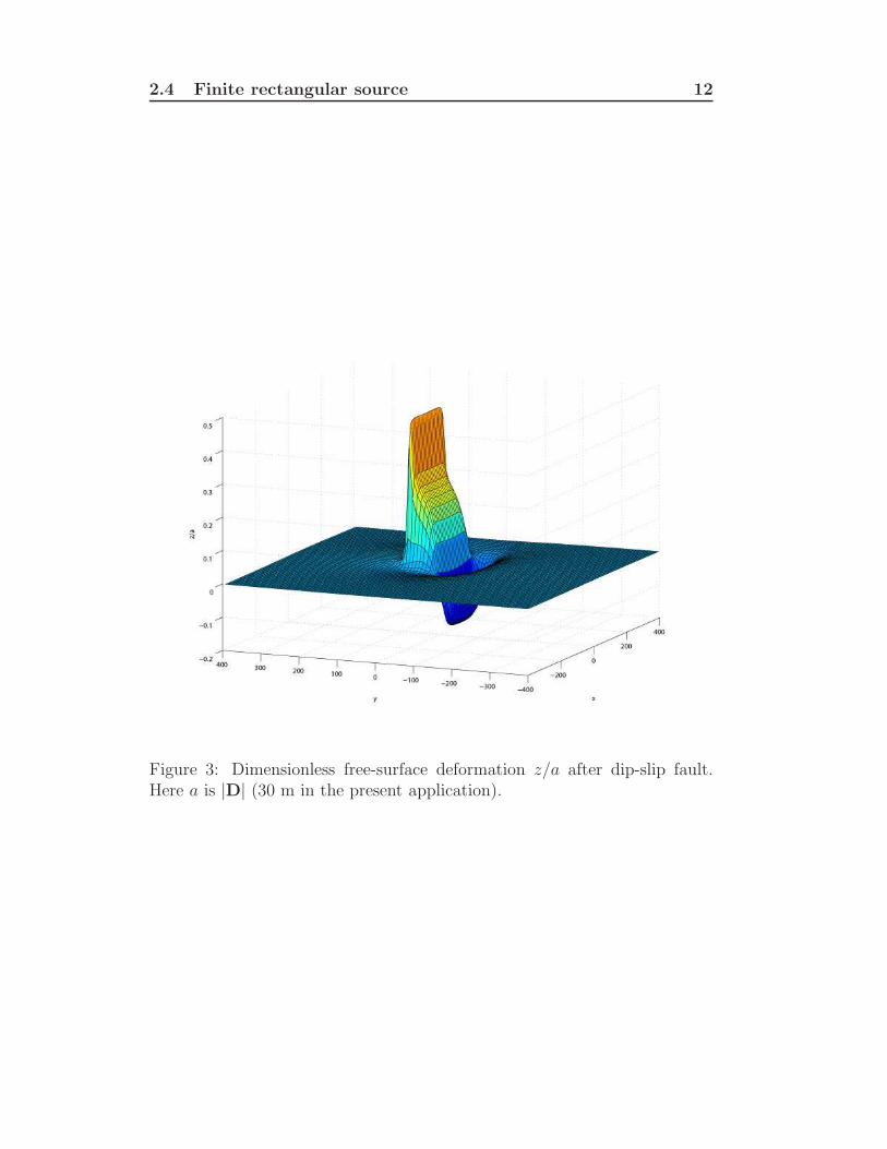
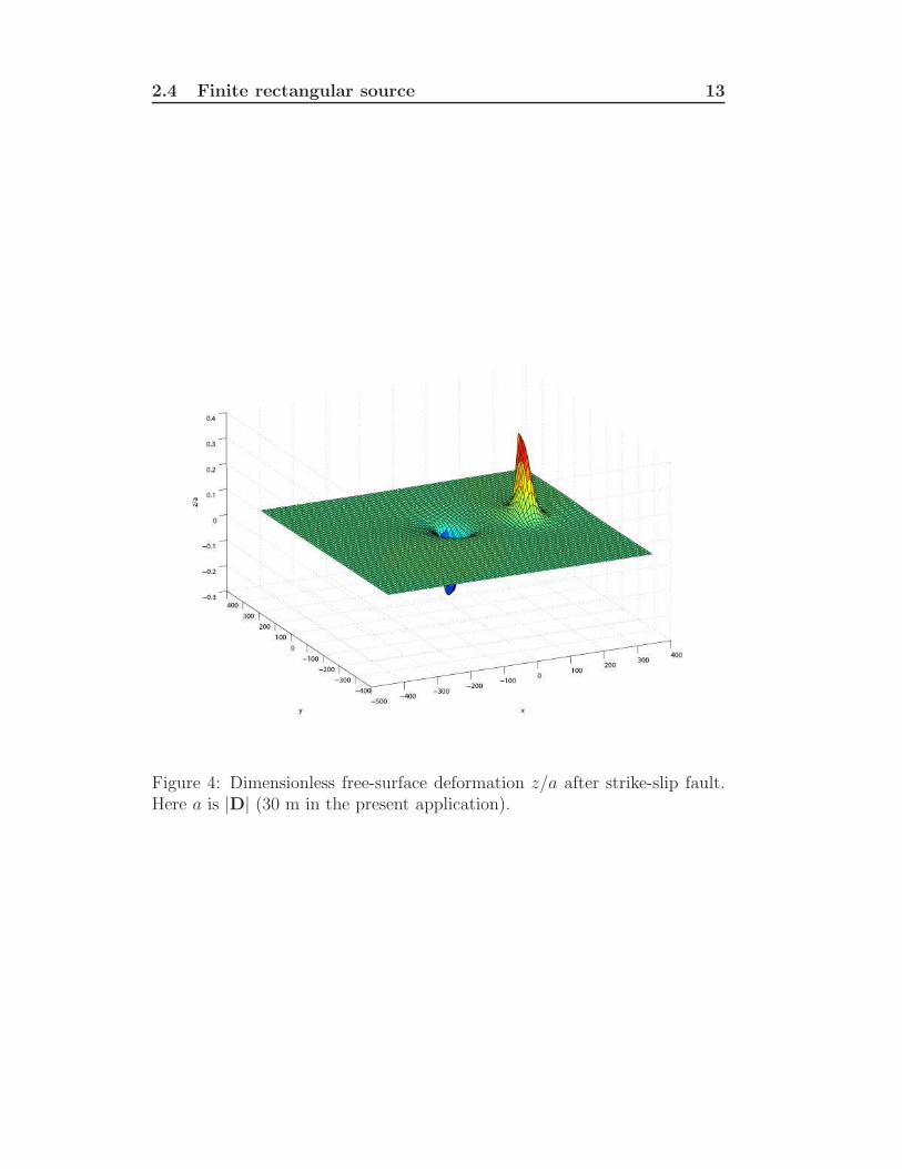
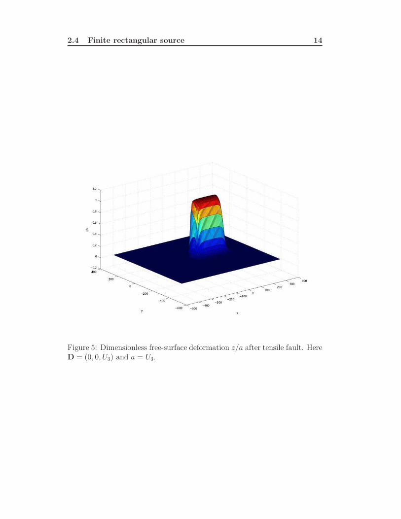
Figures 3, 4, and 5 show the free-surface deformation after three elemen-tary dislocations. The values of the parameters are given in Table 1.

The traditional approach for hydrodynamic modelers is indeed to useelastic models similar to the model just described with the seismic param-eters as input to evaluate details of the seafloor deformation. Then this

2.4 Finite rectangular source 12

Figure 3: Dimensionless free-surface deformation z/a after dip-slip fault.Here a is |D| (30 m in the present application).

2.4 Finite rectangular source 13

Figure 4: Dimensionless free-surface deformation z/a after strike-slip fault.Here a is |D| (30 m in the present application).

2.4 Finite rectangular source 14

Figure 5: Dimensionless free-surface deformation z/a after tensile fault. HereD = (0, 0, U3) and a = U3.

3 Propagation of tsunamis 15

deformation is translated to the initial condition of the evolution problemdescribed in the next section. A few authors have solved the linearized wa-ter wave equations in the presence of a moving bottom Hammack [1973],Todorovska and Trifunac [2001].

3 Propagation of tsunamis

The problem of tsunami propagation is a special case of the general water-wave problem. The study of water waves relies on several common assump-tions. Some are obvious while some others are questionable under certaincircumstances. The water is assumed to be incompressible. Dissipation isnot often included. However there are three main sources of dissipation forwater waves: bottom friction, surface dissipation and body dissipation. Fortsunamis, bottom friction is the most important one, especially in the laterstages, and is sometimes included in the computations in an ad-hoc way. Inmost theoretical analyses, it is not included.

A brief description of the common mathematical model used to studywater waves follows. The horizontal coordinates are denoted by x and y, andthe vertical coordinate by z. The horizontal gradient is denoted by

∇ :=

(

∂

∂x,

∂

∂y

)

.

The horizontal velocity is denoted by

u(x, y, z, t) = (u, v)

and the vertical velocity by w(x, y, z, t). The three-dimensional flow of aninviscid and incompressible fluid is governed by the conservation of mass

∇ · u +∂w

∂z= 0 (8)

and by the conservation of momentum

ρDu

Dt= −∇p, ρ

Dw

Dt= −ρg − ∂p

∂z. (9)

In (9), ρ is the density of water (assumed to be constant throughout the fluiddomain), g is the acceleration due to gravity and p(x, y, z, t) the pressurefield.

The assumption that the flow is irrotational is commonly made to analyzesurface waves. Then there exists a scalar function φ(x, y, z, t) (the velocitypotential) such that

u = ∇φ, w =∂φ

∂z.

3.1 Classical formulation 16

The continuity equation (8) becomes

∇2φ +∂2φ

∂z2= 0 . (10)

The equation of momentum conservation (9) can be integrated into Bernoulli’sequation

∂φ

∂t+

1

2|∇φ|2 +

1

2

(

∂φ

∂z

)2

+ gz +p − p0

ρ= 0 , (11)

which is valid everywhere in the fluid. The constant p0 is a pressure of ref-erence, for example the atmospheric pressure. The effects of surface tensionare not important for tsunami propagation.

3.1 Classical formulation

The surface wave problem consists in solving Laplace’s equation (10) in adomain Ω(t) bounded above by a moving free surface (the interface betweenair and water) and below by a fixed solid boundary (the bottom).1 The freesurface is represented by F (x, y, z, t) := η(x, y, t) − z = 0. The shape of thebottom is given by z = −h(x, y). The main driving force is gravity.

The free surface must be found as part of the solution. Two boundaryconditions are required. The first one is the kinematic condition. It can bestated as DF/Dt = 0 (the material derivative of F vanishes), which leads to

ηt + ∇φ · ∇η − φz = 0 at z = η(x, y, t) . (12)

The second boundary condition is the dynamic condition which states thatthe normal stresses must be in balance at the free surface. The normal stressat the free surface is given by the difference in pressure. Bernoulli’s equation(11) evaluated on the free surface z = η gives

φt + 12|∇φ|2 + 1

2φ2

z + gη = 0 at z = η(x, y, t) . (13)

Finally, the boundary condition at the bottom is

∇φ · ∇h + φz = 0 at z = −h(x, y) . (14)

To summarize, the goal is to solve the set of equations (10), (12), (13)and (14) for η(x, y, t) and φ(x, y, z, t). When the initial value problem is

1The surface wave problem can be easily extended to the case of a moving bottom.This extension may be needed to model tsunami generation if the bottom deformation isrelatively slow.

3.2 Dimensionless formulation 17

integrated, the fields η(x, y, 0) and φ(x, y, z, 0) must be specified at t = 0.The conservation of momentum equation (9) is not required in the solutionprocedure; it is used a posteriori to find the pressure p once η and φ havebeen found.

In the following subsections, we will consider various approximations ofthe full water-wave equations. One is the system of Boussinesq equations,that retains nonlinearity and dispersion up to a certain order. Another oneis the system of nonlinear shallow-water equations that retains nonlinearitybut no dispersion. The simplest one is the system of linear shallow-waterequations. The concept of shallow water is based on the smallness of the ratiobetween water depth and wave length. In the case of tsunamis propagatingon the surface of deep oceans, one can consider that shallow-water theory isappropriate because the water depth (typically several kilometers) is muchsmaller than the wave length (typically several hundred kilometers).

3.2 Dimensionless formulation

The derivation of shallow-water type equations is a classical topic. Twodimensionless numbers, which are supposed to be small, are introduced:

α =a

d≪ 1, β =

d2

ℓ2≪ 1, (15)

where d is a typical water depth, a a typical wave amplitude and ℓ a typicalwavelength. The assumptions on the smallness of these two numbers aresatisfied for the Indian Ocean tsunami. Indeed the satellite altimetry obser-vations of the tsunami waves obtained by two satellites that passed over theIndian Ocean a couple of hours after the rupture occurred give an amplitudea of roughly 60 cm in the open ocean. The typical wavelength estimatedfrom the width of the segments that experienced slip is between 160 and 240km Lay et al. [2005]. The water depth ranges from 4 km towards the west ofthe rupture to 1 km towards the east. These values give the following rangesfor the two dimensionless numbers:

1.5 × 10−4 < α < 6 × 10−4, 1.7 × 10−5 < β < 6.25 × 10−4. (16)

The equations are more transparent when written in dimensionless variables.The new independent variables are

x = ℓx, y = ℓy, z = dz, t = ℓt/c0, (17)

where c0 =√

gd, the famous speed of propagation of tsunamis in the openocean ranging from 356 km/h for a 1 km water depth to 712 km/h for a 4

3.3 Shallow-water equations 18

km water depth. The new dependent variables are

η = aη, h = dh, φ = gaℓφ/c0. (18)

In dimensionless form, and after dropping the tildes, the equations become

β∇2φ + φzz = 0, (19)

β∇φ · ∇h + φz = 0 at z = −h(x, y), (20)

βηt + αβ∇φ · ∇η = φz at z = αη(x, y, t), (21)

βφt + 12αβ|∇φ|2 + 1

2αφ2

z + βη = 0 at z = αη(x, y, t). (22)

So far, no approximation has been made. In particular, we have not usedthe fact that the numbers α and β are small.

3.3 Shallow-water equations

When β is small, the water is considered to be shallow. The linearizedtheory of water waves is recovered by letting α go to zero. For the shallowwater-wave theory, one assumes that β is small and expand φ in terms of β:

φ = φ0 + βφ1 + β2φ2 + · · · .

This expansion is substituted into the governing equation and the boundaryconditions. The lowest-order term in Laplace’s equation is

φ0zz = 0. (23)

The boundary conditions imply that φ0 = φ0(x, y, t). Thus the verticalvelocity component is zero and the horizontal velocity components are inde-pendent of the vertical coordinate z at lowest order. Let φ0x = u(x, y, t) andφ0y = v(x, y, t). Assume now for simplicity that the water depth is constant(h = 1). Solving Laplace’s equation and taking into account the bottomkinematic condition yields the following expressions for φ1 and φ2:

φ1(x, y, z, t) = −12(1 + z)2(ux + vy), (24)

φ2(x, y, z, t) = 124

(1 + z)4[(∇2u)x + (∇2v)y]. (25)

The next step consists in retaining terms of requested order in the free-surface boundary conditions. Powers of α will appear when expanding inTaylor series the free-surface conditions around z = 0. For example, if onekeeps terms of order αβ and β2 in the dynamic boundary condition (22) andin the kinematic boundary condition (21), one obtains

βφ0t − 12β2(utx + vty) + βη + 1

2αβ(u2 + v2) = 0, (26)

β[ηt + α(uηx + vηy) + (1 + αη)(ux + vy)] = 16β2[(∇2u)x + (∇2v)y].(27)

3.3 Shallow-water equations 19

Differentiating (26) first with respect to x and then to respect to y gives aset of two equations:

ut + α(uux + vvx) + ηx − 12β(utxx + vtxy) = 0, (28)

vt + α(uuy + vvy) + ηy − 12β(utxy + vtyy) = 0. (29)

The kinematic condition (27) can be rewritten as

ηt + [u(1 + αη)]x + [v(1 + αη)]y = 16β[(∇2u)x + (∇2v)y]. (30)

Equations (28)–(30) contain in fact various shallow-water models. The so-called fundamental shallow-water equations are obtained by neglecting theterms of order β:

ut + α(uux + vuy) + ηx = 0, (31)

vt + α(uvx + vvy) + ηy = 0, (32)

ηt + [u(1 + αη)]x + [v(1 + αη)]y = 0. (33)

Recall that we assumed h to be constant for the derivation. Going back to anarbitrary water depth and to dimensional variables, the system of nonlinearshallow water equations reads

ut + uux + vuy + gηx = 0, (34)

vt + uvx + vvy + gηy = 0, (35)

ηt + [u(h + η)]x + [v(h + η)]y = 0. (36)

This system of equations has been used for example by Titov and Syno-lakis for the numerical computation of tidal wave run-up Titov and Synolakis[1998]. Note that this model does not include any bottom friction terms. Tosolve the problem of tsunami generation caused by bottom displacement,the motion of the seafloor obtained from seismological models Okada [1985]and described in Section 3 can be prescribed during a time t0. Usually t0 isassumed to be small, so that the bottom displacement is considered as an in-stantaneous vertical displacement. This assumption may not be appropriatefor slow events.

The satellite altimetry observations of the Indian Ocean tsunami clearlyshow dispersive effects. The question of dispersive effects in tsunamis isopen. Most propagation codes ignore dispersion. A few propagation codesthat include dispersion have been developed Dalrymple et al. [2006]. A well-known code is FUNWAVE, developed at the University of Delaware over thepast ten years Kirby et al. [1998]. Dispersive shallow water-wave models arepresented next.

3.4 Boussinesq equations 20

3.4 Boussinesq equations

An additional dimensionless number, sometimes called the Stokes num-ber, is introduced:

S =α

β≈ 1. (37)

For the Indian Ocean tsunami, one finds

0.24 < S < 46. (38)

Therefore the additional assumption that S ≈ 1 may be realistic.In this subsection, we provide the guidelines to derive Boussinesq-type

systems of equations Bona et al. [2002]. Of course, the variation of bathymetryis essential for the propagation of tsunamis, but for the derivation the waterdepth will be assumed to be constant. Some notation is introduced. The po-tential evaluated along the free surface is denoted by Φ(x, y, t) := φ(x, y, η, t).The derivatives of the velocity potential evaluated on the free surface are de-noted by Φ(∗)(x, y, t) := φ∗(x, y, η, t), where the star stands for x, y, z or t.Consequently, Φ∗ (defined for ∗ 6= z) and Φ(∗) have different meanings. Theyare however related since

Φ∗ = Φ(∗) + Φ(z)η∗ .

The vertical velocity at the free surface is denoted by W (x, y, t) := φz(x, y, η, t).The boundary conditions on the free surface (12) and (13) become

ηt + ∇Φ · ∇η − W (1 + ∇η · ∇η) = 0, (39)

Φt + gη + 12|∇Φ|2 − 1

2W 2(1 + ∇η · ∇η) = 0. (40)

These two nonlinear equations provide time-stepping for η and Φ. In addi-tion, Laplace’s equation as well as the kinematic condition on the bottommust be satisfied. In order to relate the free-surface variables with the bot-tom variables, one must solve Laplace’s equation in the whole water column.In Boussinesq-type models, the velocity potential is represented as a formalexpansion,

φ(x, y, z, t) =∞∑

n=0

φ(n)(x, y, t) zn. (41)

Here the expansion is about z = 0, which is the location of the free surface atrest. Demanding that φ formally satisfy Laplace’s equation leads to a recur-rence relation between φ(n) and φ(n+2). Let φo denote the velocity potentialat z = 0, uo the horizontal velocity at z = 0, and wo the vertical velocityat z = 0. Note that φo and wo are nothing else than φ(0) and φ(1). The

3.5 Classical Boussinesq equations 21

potential φ can be expressed in terms of φo and wo only. Finally, one obtainsthe velocity field in the whole water column (−h ≤ z ≤ η) Madsen et al.[2003]:

u(x, y, z, t) = cos(z∇)uo + sin(z∇)wo, (42)

w(x, y, z, t) = cos(z∇)wo − sin(z∇)uo. (43)

Here the cosine and sine operators are infinite Taylor series operators definedby

cos(z∇) =

∞∑

n=0

(−1)n z2n

(2n)!∇2n, sin(z∇) =

∞∑

n=0

(−1)n z2n+1

(2n + 1)!∇2n+1.

Then one can substitute the representation (42)-(43) into the kinematicbottom condition and use successive approximations to obtain an explicitrecursive expression for wo in terms of uo to infinite order in h∇.

A wide variety of Boussinesq systems can been derived Madsen et al.[2003]. One can generalize the expansions to an arbitrary z−level, instead ofthe z = 0 level. The Taylor series for the cosine and sine operators can betruncated, Pade approximants can be used in operators at z = −h and/orat z = 0.

The classical Boussinesq equations are more transparent when written inthe dimensionless variables used in the previous subsection. We further as-sume that h is constant, drop the tildes, and write the equations for one spa-tial dimension (x). Performing the expansion about z = 0 leads to the van-ishing of the odd terms in the velocity potential. Substituting the expressionfor φ into the free-surface boundary conditions evaluated at z = 1 + αη(x, t)leads to two equations in η and φo with terms of various order in α and β.The small parameters α and β are of the same order, while η and φo as wellas their partial derivatives are of order one.

3.5 Classical Boussinesq equations

The classical Boussinesq equations are obtained by keeping all terms thatare at most linear in α or β. In the derivation of the fundamental non-linear shallow-water equations (31)–(33), the terms in β were neglected. Itis therefore implicitly assumed that the Stokes number is large. Since thecube of the water depth appears in the denominator of the Stokes number(S = α/β = aℓ2/d3), it means that the Stokes number is 64 times larger in a1 km depth than in a 4 km depth! Based on these arguments, dispersion is

3.6 Korteweg–de Vries equation 22

more important to the west of the rupture. Considering the Stokes numberto be of order one leads to the following system in dimensional form2:

ut + uux + gηx − 12h2utxx = 0, (44)

ηt + [u(h + η)]x − 16h3uxxx = 0. (45)

The classical Boussinesq equations are in fact slightly different. They areobtained by replacing u with the depth averaged velocity

1

h

∫ η

−h

u dz.

They read

ut + uux + gηx − 13h2utxx = 0, (46)

ηt + [u(h + η)]x = 0. (47)

A number of variants of the classical Boussinesq system were studied byBona et al., who in particular showed that depending on the modeling ofdispersion the linearization about the rest state may or may not be well-posed Bona et al. [2002].

3.6 Korteweg–de Vries equation

The previous system allows the propagation of waves in both the positiveand negative x−directions. Seeking solutions travelling in only one direction,for example the positive x−direction, leads to a single equation for η, theKorteweg–de Vries equation:

ηt + c0

(

1 +3η

2d

)

ηx +1

6c0d

2ηxxx = 0, (48)

where d is the water depth. It admits solitary wave solutions travelling atspeed V in the form

η(x, t) = a sech2

(

√

3a

4d3(x − V t)

)

, with V = c0

(

1 +a

2d

)

.

The solitary wave solutions of the Korteweg–de Vries equation are of elevation(a > 0) and travel faster than c0. Their speed increases with amplitude. Notethat a natural length scale appears:

ℓ =

√

4d3

3a.

2Equations (44) and (45) could have been obtained from equations (28) and (30).

4 Energy of a tsunami 23

For the Indian Ocean tsunami, it gives roughly ℓ = 377 km. It is of the orderof magnitude of the wavelength estimated from the width of the segmentsthat experienced slip.

4 Energy of a tsunami

The energy of the earthquake is measured via the strain energy releasedby the faulting. The part of the energy transmitted to the tsunami wave isless than one percent Lay et al. [2005]. They estimate the tsunami energy tobe 4.2×1015 J. They do not give details on how they obtained this estimate.However, a simple calculation based on considering the tsunami as a soliton

η(x) = a sech2(x

ℓ

)

, u(x) = αc0 sech2(x

ℓ

)

,

gives for the energy

E =1√3α3/2ρd2(c2

0 + gd)

∫

∞

−∞

sech4x dx + O(α2).

The value for the integral is 4/3. The numerical estimate for E is close tothat of Lay et al. (2005). Incidently, at this level of approximation, thereis equipartition between kinetic and potential energy. It is also importantto point out that a tsunami being a shallow water wave, the whole watercolumn is moving as the wave propagates. For the parameter values used sofar, the maximum horizontal current is 3 cm/s. However, as the water depthdecreases, the current increases and becomes important when the depth be-comes less than 500 m. Additional properties of solitary waves can be foundfor example in Longuet-Higgins [1974].

5 Tsunami run-up

The last phase of a tsunami is its run-up and inundation. Although insome cases it may be important to consider the coupling between fluid andstructures, we restrict ourselves to the description of the fluid flow. Theproblem of waves climbing a beach is a classical one Carrier and Greenspan[1958]. The transformations used by Carrier and Greenspan are still usednowadays. The basis of their analysis is the one-dimensional counterpart ofthe system (34)–(36). In addition, they assume the depth to be of uniformslope: h = −x tan θ. Introduce the following dimensionless quantities, where

5 Tsunami run-up 24

ℓ is a characteristic length3:

x = ℓx, η = ℓη, u =√

gℓ u, t =√

ℓ/g t, c2 = (h + η)/ℓ.

After dropping the tildes, the dimensionless system of equations (34)-(36)becomes

ut + uux + ηx = 0,

ηt + [u(−x tan θ + η)]x = 0.

In terms of the variable c, these equations become

ut + uux + 2ccx + tan θ = 0,

2ct + cux + 2ucx = 0.

The equations written in characteristic form are[

∂

∂t+ (u + c)

∂

∂x

]

(u + 2c + t tan θ) = 0,

[

∂

∂t+ (u − c)

∂

∂x

]

(u − 2c + t tan θ) = 0.

The characteristic curves C+ and C− as well as the Riemann invariants are

C+ :dx

dt= u + c, u + 2c + t tan θ = r,

C− :dx

dt= u − c, u − 2c + t tan θ = s.

Next one can rewrite the hyperbolic equations in terms of the new variablesλ and σ defined as follows:

λ

2=

1

2(r + s) = u + t tan θ,

σ

4=

1

4(r − s) = c.

One obtains

xs −[

1

4(3r + s) − t tan θ

]

ts = 0,

xr −[

1

4(r + 3s) − t tan θ

]

tr = 0.

3In fact there is no obvious characteristic length in this idealized problem. Some authorssimply say at this point that ℓ is specific to the problem under consideration.

5 Tsunami run-up 25

The elimination of x results in the linear second-order equation for t

σ(tλλ − tσσ) − 3tσ = 0. (49)

Since u + t tan θ = λ/2, u must also satisfy (49). Introducing the potentialφ(σ, λ) such that

u =φσ

σ,

one obtains the equation

(σφσ)σ − σφλλ = 0

after integrating once. Two major simplifications have been obtained. Thenonlinear set of equations have been reduced to a linear equation for u or φand the free boundary is now the fixed line σ = 0 in the (σ, λ)−plane. Thefree boundary is the instantaneous shoreline c = 0, which moves as a waveclimbs a beach.

The above formulation has been used by several authors to study therun-up of various types of waves on sloping beaches Carrier et al. [2003],Tadepalli and Synolakis [1994], Tinti and Tonini [2005]. For example, it hasbeen shown that leading depression N -waves run-up higher than leadingelevation N -waves, suggesting that perhaps the solitary wave model maynot be adequate for predicting an upper limit for the run-up of near-shoregenerated tsunamis.

There is a rule of thumb that says that the run-up does not usually exceedtwice the fault slip. Since run-ups of 30 meters were observed in Sumatraduring the Boxing Day tsunami, the slip might have been of 15 meters oreven more.

Analytical models are useful, especially to perform parametric studies.However, the breaking of tsunami waves as well as the subsequent floodingsmust be studied numerically. The most natural methods that can be used arethe free surface capturing methods based on a finite volume discretisation,such as the Volume Of Fluid (VOF) or the Level Set methods, and the familyof Smoothed Particle Hydrodynamics methods (SPH), applied to free-surfaceflow problems Gomez-Gesteira et al. [2005], Gomez-Gesteira and Dalrymple[2004], Monaghan [1994]. Such methods allow a study of flood wave dynam-ics, of wave breaking on the land behind beaches, and of the flow over risingground with and without the presence of obstacles. This task is an essentialpart of tsunami modelling, since it allows the determination of the level ofrisk due to major flooding, the prediction of the resulting water levels in theflooded areas, the determination of security zones. It also provides some helpin the conception and validation of protection systems in the most exposedareas.

6 Direction for future research 26

6 Direction for future research

A useful direction for future research in the dynamics of tsunami waves isthe three-dimensional (3D) simulation of tsunami breaking along a coast. Forthis purpose, different validation steps are necessary. First more simulationsof a two-dimensional (2D) tsunami interacting with a sloping beach oughtto be performed. Then these simulations should be extended to the case ofa 2D tsunami interacting with a sloping beach in the presence of obstacles.An important output of these computations will be the hydrodynamic load-ing on obstacles. The nonlinear inelastic behaviour of the obstacles may beaccounted for using damage or plasticity models. The development of Boussi-nesq type models coupled with structure interactions is also a promising task.Finally there is a need for 3D numerical simulations of a tsunami interact-ing with a beach of complex bathymetry, with or without obstacles. Thesesimulations will hopefully demonstrate the usefulness of numerical simula-tions for the definition of protecting devices or security zones. An importantchallenge in that respect is to make the numerical methods capable of han-dling interaction problems involving different scales: the fine scale needed forrepresenting the damage of a flexible obstacle and a coarse scale needed toquantify the tsunami propagation.

References

A. Ben-Mehanem, S. J. Singh, and F. Solomon. Deformation of an homo-geneous earth model finite by dislocations. Rev. Geophys. Space Phys., 8:591–632, 1970. 4

A. Ben-Menahem, S. J. Singh, and F. Solomon. Static deformation of aspherical earth model by internal dislocations. Bull. Seism. Soc. Am., 59:813–853, 1969. 4

J. L. Bona, M. Chen, and J.-C. Saut. Boussinesq equations and other systemsfor small-amplitude long waves in nonlinear dispersive media. i: Derivationand linear theory. Journal of Nonlinear Science, 12:283–318, 2002. 20, 22

G. F. Carrier and H. P. Greenspan. Water waves of finite amplitude on asloping beach. Journal of Fluid Mechanics, 2:97–109, 1958. 23

G. F. Carrier, T. T. Wu, and H. Yeh. Tsunami run-up and draw-down on aplane beach. Journal of Fluid Mechanics, 475:79–99, 2003. 25

REFERENCES 27

H. Chanson. Le tsunami du 26 decembre 2004: un phenomene hydrauliqued’ampleur internationale. premiers constats. La Houille Blanche, 2:25–32,2005. 2

M. A. Chinnery. The stress changes that accompany strike-slip faulting. Bull.

Seism. Soc. Am., 53:921–932, 1963. 9

R. A. Dalrymple, S. T. Grilli, and J. T. Kirby. Tsunamis and challenges foraccurate modeling. Oceanography, 19:142–151, 2006. 19

M. Gomez-Gesteira, D. Cerqueiro, C. Crespo, and R. A. Dalrymple. Greenwater overtopping analyzed with a sph model. Ocean Engineering, 32:223–238, 2005. 25

M. Gomez-Gesteira and R. A. Dalrymple. Using sph for wave impact on a tallstructure. Journal of Waterways, Port, Coastal, and Ocean Engineering,130:63–69, 2004. 25

J. Hammack. A note on tsunamis: their generation and propagation in anocean of uniform depth. Journal of Fluid Mechanics, 60:769–799, 1973. 15

J. Hunt and J. M. Burgers. Tsunami waves and coastal flooding. Mathematics

TODAY, pages 144–146, October 2005. 3

T. Iwasaki and R. Sato. Strain field in a semi-infinite medium due to aninclined rectangular fault. J. Phys. Earth, 27:285–314, 1979. 9

J. T. Kirby, G. Wei, Q. Chen, A. B. Kennedy, and R. A. Dalrymple. Fun-wave 1.0, fully nonlinear boussinesq wave model documentation and user’smanual. Research Report No. CACR-98-06, 1998. 19

T. Lay, H. Kanamori, C. J. Ammon, M. Nettles, S. N. Ward, R. C. Aster, S. L.Beck, S. L. Bilek, M. R. Brudzinski, R. Butler, H. R. DeShon, G. Ekstrom,K. Satake, and S. Sipkin. The great sumatra-andaman earthquake of 26december 2004. Science, 308:1127–1133, 2005. 17, 23

M. S. Longuet-Higgins. On the mass, momentum, energy and circulation ofa solitary wave. Proc. R. Soc. Lond. A, 337:1–13, 1974. 23

A. E. H. Love. A treatise on the mathematical theory of elasticity. DoverPublications, New York, 1944. 5, 7

P. A. Madsen, H. B. Bingham, and H. A. Schaffer. Boussinesq-type formula-tions for fully nonlinear and extremely dispersive water waves: derivationand analysis. Proc. R. Soc. Lond. A, 459:1075–1104, 2003. 21

REFERENCES 28

T. Maruyama. Statical elastic dislocations in an infinite and semi-infinitemedium. Bull. Earthquake Res. Inst., Tokyo Univ., 42:289–368, 1964. 6

T. Masterlark. Finite element model predictions of static deformation fromdislocation sources in a subduction zone: Sensivities to homogeneous,isotropic, poisson-solid, and half-space assumptions. J. Geophys. Res.,108(B11):2540, 2003. 4

J. R. McGinley. A comparison of observed permanent tilts and strains due to

earthquakes with those calculated from displacement dislocations in elastic

earth models. PhD thesis, California Institute of Technology, Pasadena,California, 1969. 4

R. D. Mindlin. Force at a point in the interior of a semi-infinite medium.Physics, 7:195–202, 1936. 6, 7

R. D. Mindlin and D. H. Cheng. Nuclei of strain in the semi-infinite solid.J. Appl. Phys., 21:926–930, 1950. 6

J. J. Monaghan. Simulating free surface flows with sph. Physica D, 110:399–406, 1994. 25

Y. Okada. Surface deformation due to shear and tensile faults in a half-space.Bull. Seism. Soc. Am., 75:1135–1154, 1985. 3, 7, 9, 19

Y. Okada. Internal deformation due to shear and tensile faults in a half-space.Bull. Seism. Soc. Am., 82:1018–1040, 1992. 7, 9

F. Press. Displacements, strains and tilts at tele-seismic distances. J. Geo-

phys. Res., 70:2395–2412, 1965. 6, 7

R. Sato and M. Matsu’ura. Strains and tilts on the surface of a semi-infinitemedium. J. Phys. Earth, 22:213–221, 1974. 9

D. E. Smylie and L. Mansinha. The elasticity theory of dislocations in realearth models and changes in the rotation of the earth. Geophys. J.R. Astr.

Soc., 23:329–354, 1971. 4

I. S. Sokolnikoff and R. D. Specht. Mathematical theory of elasticity.McGraw-Hill, New York, 1946. 5

J. A. Steketee. On volterra’s dislocation in a semi-infinite elastic medium.Can. J. Phys., 36:192–205, 1958. 3, 4

REFERENCES 29

S. Tadepalli and C. E. Synolakis. The run-up of n-waves on sloping beaches.Proc. R. Soc. Lond. A, 445:99–112, 1994. 25

S. Tinti and R. Tonini. Analytical evolution of tsunamis induced by near-shore earthquakes on a constant-slope ocean. Journal of Fluid Mechanics,535:33–64, 2005. 25

V. V. Titov and C. E. Synolakis. Numerical modeling of tidal wave runup.J. Waterway, Port, Coastal, and Ocean Engineering, 124:157–171, 1998.19

M. I. Todorovska and M. D. Trifunac. Generation of tsunamis by a slowlyspreading uplift of the seafloor. Soil Dynamics and Earthquake Engineer-

ing, 21:151–167, 2001. 15

V. Volterra. Sur l’equilibre des corps elastiques multiplement connexes. An-

nales Scientifiques de l’Ecole Normale Superieure, 24(3):401–517, 1907. 4,5

H. M. Westergaard. Bull. Amer. Math. Soc., 41:695, 1935. 6