Early Protostellar Evolution

Challenges for star formation observations & theory

Stella OffnerHubble Fellow

Mike Dunham

Yale UniversityFrontiers in Star Formation, Oct 27, 2012

&

protostellar luminosities are a window to instantaneous star formation processes (accretion, masses, time-dependence, duration, big picture)

Solution: to understand early protostellar evolution

study a different observational metric:

Motivation

Chabrier 05

The IMF is universal

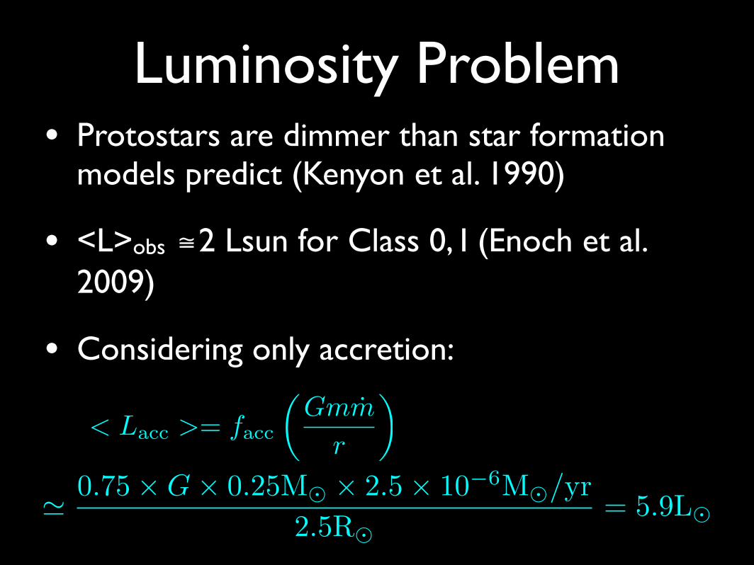
Luminosity Problem• Protostars are dimmer than star formation

models predict (Kenyon et al. 1990)

• <L>obs ≅2 Lsun for Class 0, I (Enoch et al. 2009)

• Considering only accretion:

< Lacc >= facc

✓Gmm

r

◆

Observational Challenges• Identify protostars

• SEDs show great diversity

• Obtain >3 order of mag. wavelength coverage

• Extinction Corrections

• What is Lbol?

Jorgensen et al.

What are the key observations?

• What are the mean and median luminosities?

• What is the total range of luminosities?

• How are Class 0/1 luminosities different? (Or are they?)

• How low do they go?

Mean and Median Luminosities

• Mean:Lbol = 4.3 Lsun (5.8 Lsun) (c2d+GB; Dunham et al. 2012)

• Median:Lbol = 1.3 Lsun (1.8 Lsun) (c2d+GB; Dunham et al. 2012)

Range of Luminosities

• 0.01 - 69 Lsun

• >3 orders of magnitude(3.8 dex)

Dunham et al. (2012)

Class 0 vs. Class I

• Mean:4.5 Lsun (Class 0)3.8 Lsun (Class I)

• Median:1.4 Lsun (Class 0)1.0 Lsun (Class I)

• Lbol < 0.5 Lsun:20% (Class 0)36% (Class I)

• K-S test: 0.04

Dunham et al. (2012)

How low do they go?

Dunham et al. (2008)

Chen et al. (2010)Enoch et al. (2010)Pineda et al. (2011)

Dunham et al. (2011)Schnee et al. (2012)Chen et al. (2012)

Pezzuto et al. (2012)

What does it all imply?• What is the underlying star formation theory (e.g.

Turbulent Core, Competitive Accretion)?• What is the underlying star formation theory (e.g.

Turbulent Core, Competitive Accretion)?

• What is the role of episodic accretion (i.e. importance of disks)?

Offner et al. 09 yt

• What is the underlying star formation theory (e.g. Turbulent Core, Competitive Accretion)?

• What is the role of episodic accretion (i.e. importance of disks)?

• How does (de)accelerating star formation or early/delayed high-mass star formation fit in?

Stahler & Palla 2000

Protostellar Mass & Luminosity Functions (PMF, PLF)

Star Formation

Obs IMF

Models: dm/dt

PMF

Models: L(m,mf)

PLF

• Isothermal Sphere (IS), Shu 77

• Turbulent Core (TC), McKee & Tan 03

• Competitive Accretion (CA), Bonnell et al. 97

• 2-Component Models (IS+TC, IS+CA) Offner & McKee (2011)McKee & Offner (2010)

Star Formation Models

The Protostellar Luminosity Function 9

Fig. 4.— Protostellar lifetime estimated using the observed meanluminosity from the Evans et al. (2009) data as a function of themean luminosity from the models. The error bars on the modellifetimes derive from the observal luminosity uncertainty. The twoobservational results with uncertainty are shown by the thick setof solid error bars.

Fig. 5.— The PLF for mu = 3M� for untapered, non-accelerating star formation (top) and untapered, accelerating starformation with � = 1 Myr (bottom). The observed PLF (Evanset al. 2009) is plotted for comparison. Note that the PLF shapeis derived assuming that the accretion luminosity dominates thetotal.

complete observations of high-mass star-forming regionswould be useful to distinguish models based solely uponthe mean luminosity. Note that the model means dependupon the uncertain star-formation timescale, so that it isnot possible to make an independent comparison of themodels and observations (see discussion in §5). However,better constraints on the star formation time in the fu-

Fig. 6.— The PLF for mu = 3M� with tapered accretion rates.The observed PLF (Evans et al. 2009) is plotted for comparison.Note that the PLF shape is derived assuming that the accretionluminosity dominates the total.

ture should increase the discriminating value of the meanluminosity in comparing models.

As shown in the plot insets, the mean observed lumi-nosity falls above the models in all the non-acceleratingcases cases. The untapered TC and CA means, IS ta-pered mean, and all accelerating means are consistentwith the observational error.1 This clearly indicates thatthere is no luminosity problem in the traditional sense.The resolution is a result of the longer protostellar life-time adopted from Evans et al. (2009) and an e�ectiveaccretion e⇤ciency, facc, e� = 0.56 due to a radiative ef-ficiency of 75% and allowance for episodic accretion atthe level of 25%. Altogether this reduces the predictedluminosities for the non-accelerating cases by a factor of� 3.

The mean luminosities in the accelerating cases areup to 30% lower than in the fiducial non-acceleratingcases for a fixed value of ⇤tf ⌅ because the acceleratingcases have more low-mass protostars. However, for agiven observed value of ⇤tf ⌅obs, the mean luminositiesare raised since their formation time is a factor ⇥ 2.3smaller, as shown in equation (25). It is this adjustmentthat accounts for the good agreement of the acceleratingmodels with the observations.

Allowing the accretion rates to taper o� during theaccretion period has a varying e�ect on the mean lumi-

1 The CA luminosity distribution extends to both the highestand the lowest luminosities, so that it yields the largest mean whena cuto� of 0.05L� is applied and the curve is re-normalized thusweighting the highest luminosities more heavily; the IS case is leasta�ected by this luminosity truncation since it is strongly peakedaround a luminosity much higher than the cuto�.

L (Lsun)

(Evans ea 09)

Protostellar Luminosity Function (PLF)

TC, CA are better models: constant star

formation times (i.e. accretion increases with

final mass)

Offner & McKee 2011

Isothermal SphereTwo-Component Turbulent CoreTurbulent CoreCompetitive Accretion

Estimating Episodic Accretion• Np = # of bursting sources = 20 (observed in last 70 yr)

• N* = Star Formation Rate = 0.016*/yr

• <mf> = 0.5 Msun

�thigh =Np

N⇤=

200.016 ⇤ /yr

' 1200 yr

fepi =mhigh�thigh

< mf >=

10�4M�/yr 1200yr0.5M�

' 0.25

Nb⇤ =0.2 bursts/yr0.016 ⇤ /yr

' 10 bursts tb⇤ =1200 yr

10 bursts' 100 yr

1/4 of Mass

0.1-1% of acc. time

B m

ag Kenyon & Hartman 96

FU Ori

Offner & McKee 2011

Star Formation Models

The Protostellar Luminosity Function 9

Fig. 4.— Protostellar lifetime estimated using the observed meanluminosity from the Evans et al. (2009) data as a function of themean luminosity from the models. The error bars on the modellifetimes derive from the observal luminosity uncertainty. The twoobservational results with uncertainty are shown by the thick setof solid error bars.

Fig. 5.— The PLF for mu = 3M� for untapered, non-accelerating star formation (top) and untapered, accelerating starformation with � = 1 Myr (bottom). The observed PLF (Evanset al. 2009) is plotted for comparison. Note that the PLF shapeis derived assuming that the accretion luminosity dominates thetotal.

complete observations of high-mass star-forming regionswould be useful to distinguish models based solely uponthe mean luminosity. Note that the model means dependupon the uncertain star-formation timescale, so that it isnot possible to make an independent comparison of themodels and observations (see discussion in §5). However,better constraints on the star formation time in the fu-

Fig. 6.— The PLF for mu = 3M� with tapered accretion rates.The observed PLF (Evans et al. 2009) is plotted for comparison.Note that the PLF shape is derived assuming that the accretionluminosity dominates the total.

ture should increase the discriminating value of the meanluminosity in comparing models.

As shown in the plot insets, the mean observed lumi-nosity falls above the models in all the non-acceleratingcases cases. The untapered TC and CA means, IS ta-pered mean, and all accelerating means are consistentwith the observational error.1 This clearly indicates thatthere is no luminosity problem in the traditional sense.The resolution is a result of the longer protostellar life-time adopted from Evans et al. (2009) and an e�ectiveaccretion e⇤ciency, facc, e� = 0.56 due to a radiative ef-ficiency of 75% and allowance for episodic accretion atthe level of 25%. Altogether this reduces the predictedluminosities for the non-accelerating cases by a factor of� 3.

The mean luminosities in the accelerating cases areup to 30% lower than in the fiducial non-acceleratingcases for a fixed value of ⇤tf ⌅ because the acceleratingcases have more low-mass protostars. However, for agiven observed value of ⇤tf ⌅obs, the mean luminositiesare raised since their formation time is a factor ⇥ 2.3smaller, as shown in equation (25). It is this adjustmentthat accounts for the good agreement of the acceleratingmodels with the observations.

Allowing the accretion rates to taper o� during theaccretion period has a varying e�ect on the mean lumi-

1 The CA luminosity distribution extends to both the highestand the lowest luminosities, so that it yields the largest mean whena cuto� of 0.05L� is applied and the curve is re-normalized thusweighting the highest luminosities more heavily; the IS case is leasta�ected by this luminosity truncation since it is strongly peakedaround a luminosity much higher than the cuto�.

L (Lsun)

(Evans ea 09)

Offner & McKee 2011

Protostellar Luminosity Function (PLF)

TC, CA are better models: constant star

formation times (i.e. accretion increases with

final mass)

Isothermal SphereTwo-Component Turbulent CoreTurbulent CoreCompetitive Accretion

“Episodic” vs. Variable Accretion

L (Lsun)

dm/dt can vary by a factor of 2

Offner & McKee in prep.

Add random variations on top of accretion IS trend:

by a factor of 10

Question: How much time

variability occurs?

Second Approach:Modeling Individual Cores

Vorobyov & Basu (2005, 2006, 2010)

• Hydro simulations of collapsing cores

• Resolve disk physics(but not inner disk < 6 AU)

• Variable, episodic accretion dependent on initial conditions

Assemble models over range of IC

Post-process with continuum rad. trans.

Generate synthetic obs., measure Lbol

Weight over inclinations, IMF

Second Approach:Modeling Individual Cores

Dunham & Vorobyov (2012)

Conclusions• Protostars in local regions have a mean luminosity of

~4.3 Lsun and extend over 3 order of magnitude

• Class 0 & Class 1s have similar luminosities but there are more low luminosity Class 1s

• Many candidate first cores exist but require confirmation

• Episodic accretion could account for ~1/4 of a star’s mass but probably <1% of accretion time.

• Observations can be explained by some combination of longer accretion, episodic/variable accretion, and mass-dependent accretion