Embed Size (px)
Citation preview

1
Earth Observations for Official
Statistics
Satellite Imagery and Geospatial Data
Task Team report
5th December 2017
White cover publication, pre-edited text subject to official editing and subject to further consultation
United Nations
Australian Bureau of Statistics
Queensland University of Technology, Australia
Queensland Government, Australia
Commonwealth Scientific and Industrial Research Organisation, Australia
European Commission – DG Eurostat
National Institute of Statistics and Geography, Mexico
Statistics Canada

2
Executive summary
This handbook, written by members of the United Nations Task Team on Satellite Imagery and Geo-
spatial Data, provides a guide for National Statistical Offices considering using satellite imagery
(known as earth observations) data for official statistics. It was produced as an input to the United
Nation Global Working Group on Big Data for Official Statistics report to the United Nations Statistical
Commission for 2017.
The handbook provides a brief introduction to the use of earth observations (EO) data for official
statistics, types of sources available and methodologies for producing statistics from this type of data.
It also summarises the results of four pilot projects produced by Task Team members; Australian Bureau
of Statistics (ABS), Australia, Instituto Nacional de Estadística Geografíca e Informática (INEGI),
Mexico, Departamento Administrativo Nacional de Estadistica (DANE), Colombia and Google.
Supplementary material includes a methodology literature review, and the full reports of the pilot
projects.
In the final chapter, guidelines are presented for National Statistical Offices to consider and refer to
when considering whether to implement earth observations data sources into their statistical production
process, and issues to consider throughout the implementation and output processes. Rather than being
prescriptive, the guidelines are intended to prompt National Statistical Office to critically consider their
own business needs, and apply the recommendations as appropriate to their circumstances. As the
international experience using these data for statistical purposes grows, National Statistical Offices can
build on the guidelines provided in this handbook with their own expertise and knowledge.

3
Foreword
Official statisticians have been using a diversity of data sources in the production of official statistics
for decades, including “designed” data sources such as censuses and surveys, and “found” data sources
such as administrative and transactional data.
As a result of increasing interaction with digital technologies by citizens, and the increasing capability
of these technologies to provide digital trails, new sources of data have emerged and are increasingly
available to official statisticians. Such sources include data from sensor networks and tracking devices
e.g. satellites and mobile phones.
Statistical agencies around the world have a strong interest in exploring the viability of using satellite
imagery data, or more broadly termed as earth observations (EO) data, to improve official statistics on
a wide range of topics spanning agriculture, the environment, business activity and transport.
EO data have significant potential to provide more timely statistical outputs, to reduce the frequency of
surveys, to reduce respondent burden and other costs, to provide data at a more disaggregated level for
informed decision making and to provide new statistics and statistical insights.
EO data may also support the monitoring of the Sustainable Development Goals (SDGs) by improving
timeliness and relevance of indicators without compromising their impartiality and methodological
soundness.
This handbook provides a brief introduction to the use of EO data for official statistics, types of sources
available, examples of using EO data to compile the indicators for SDGs and methodologies for
producing statistics from this type of data. It also summarises the results of four pilot projects produced
by United Nations Satellite Imagery and Geospatial Data Task Team members to explore the feasibility
of using EO data for official statistics, and additionally, other relevant and useful case studies.
Supplementary material includes a methodology literature review.
In the final chapter, guidelines are presented for National Statistical Offices to consider and refer to
when considering whether to use EO data in producing official statistics, and issues to consider
throughout the implementation and output processes.
Producing this handbook would not have been possible without the hard work, dedication and
significant contributions of the chapter authors. I would like to express my appreciation to Dr Hannes
I. Reuter (Eurostat), Dr Arnold Dekker, Flora Kerblat, Dr Alex Held and Dr Robert Woodcock
(Commonwealth Science and Industrial Research Organisation) Alexis McIntyre (Geoscience
Australia), Professor Kerrie Mengersen and James McBroom (Queensland University of Technology),
Sandra Yaneth Rodriquez (Departamento Administrativo Nacional de Estadistica), and Jacinta
Holloway (Australian Bureau of Statistics). I would also like to thank the authors of the Task Team
Pilot reports, Patrick Dunagan (Google), Ronaldo Ocampo and José De La Torre (Instituto Nacional
de Estadística Geografíca e Informática), Jennifer Marley, Ryan Defina, Kate Traeger, Daniel Elazar,
Anura Amarasinghe and Gareth Biggs (Australian Bureau of Statistics). Thank you also to Ben
Fitzpatrick and Brigitte Colin (Queensland University of Technology) for their contributions to the
methods case studies in Chapter 4. Thank you also to Statistics Canada for allowing us to include their
work as an example of using EO data for official statistics in practice.

4
Receiving comments and feedback from experts in the earth science, statistical methodology,
agriculture and geospatial fields has been essential to producing this handbook. I would also like to
thank Sybille McKeown, Daniel Elazar, Martin Brady and Thomas Walter (Australian Bureau of
Statistics), Alexis McIntyre (Geoscience Australia), Dr Andries Potgieter (University of Queensland),
Dr Matthew Pringle and Dr Michael Schmidt (Queensland Department of Science, Information
Technology and Innovation), Dr Giulia Conchedda and Jacques Delincé (Food and Agriculture
Organization of the United Nations) and Javier Gallego (Joint Research Center - European
Commission) for their comments and suggestions to improve the handbook content.
Dr Siu-Ming Tam
Chair, United Nations Satellite Imagery and Geo-spatial Data Task Team
5
1. Introduction
Remote sensing is a technology that aims to observe and study the Earth systems, and their dynamics.
Data related to remote sensing, specifically satellite images, have a purpose to observe and study the
Earth from space; its land surface, the oceans and the atmosphere (ESA, 2016)1. Civilisation interacts
with the natural components of Earth systems, adapting them in diverse and complex ways, generating
modified Earth systems suitable for measuring by Earth Observation (EO).
In this sense, what society does, and its relation with Earth, has different responses which modify
geospatial variables. These can be directly or indirectly detected by EO; indeed, socio-economic activity
is distributed across most of the planet. Then, if the National Statistical Offices (NSOs) are among the
most important sources of basic socio-economic information for their Governments, EO data and
information is a key geospatial source that complements, improves and updates official statistics. This
means a change of paradigm from past and current statistical approaches measuring effects of social
life on Earth (anthropogenic effects), its evolution, distribution, impacts and sustainability. Basically,
the main challenges that mankind is facing in what is now called the Anthropocene.
EO data and the information derived from these data is a special case of geospatial Big Data. Big Data
is defined as “any large and complex collection of data sets that becomes difficult to process using
traditional data processing applications”, and therefore includes data from EO satellites. In many cases,
Big Data is considered to be unstructured data or data that is used for another aim than the original
creator of the data intended. In the case of EO it is actually purposefully created to be highly structured
and to measure specific aspects of the Earth. The complexity of EO data is to extract meaningful
information about a real object, value, state or condition from its reflected or emitted electromagnetic
signal coming from the earth, the atmosphere or ocean, travelling through the atmosphere and measured
in space, ocean or soil.
Satellite EO as an information source in support of many sectors of government and industry has been
proven, and was reconfirmed in September 2015 by world leaders, whilst adopting the 2030 Agenda
for Sustainable Development. They recognised the critical importance of “transparent and accountable
scaling-up of appropriate public-private cooperation to exploit the contribution to be made by a wide
range of data, including EO and geospatial information, while ensuring national ownership in
supporting and tracking progress”. In adopting the 2030 Agenda for Sustainable Development, world
leaders agreed that a global indicator framework would be an essential tool to measure, monitor and
report progress on achieving the Sustainable Development Goals (SDGs). At the 47th Session of the
United Nations Statistical Commission (UNSC) 8-11 March 2016, global indicators were presented and
discussed to help NSOs to monitor these 17 SDGs. Effective use of the information in satellite imagery
can have a transformational impact on many of humanity’s most significant challenges, such as helping
global scientists, resource and planning managers and politicians better monitor and protect fragile
ecosystems, ensure resilient infrastructure, manage climate risks, enhance food security, build more
resilient cities, reduce poverty, and improve governance, among others.
The Global Working Group (GWG) on Big Data for Official Statistics was created in 2014, as an
outcome of the 45th meeting of the UN Statistical Commission. In accordance with its terms of
reference, the UN GWG provides strategic vision, direction and coordination of a global programme
on Big Data for official statistics, including for indicators of the 2030 agenda for sustainable
1 http://www.esa.int/SPECIALS/Eduspace_EN/SEMF9R3Z2OF_0.html

6
development. It also promotes practical use of Big Data sources, while promoting capability building,
training and sharing of experiences.
Finally, UN GWG fosters communication and advocacy of use of Big Data for policy applications and
offers advice in building public trust in the use of Big Data from the private sector.
In this context, this report focuses on EO data and methods as explored by the UN GWG Task Team
on Satellite Imagery and Geo-Spatial Data.
In the past the uptake by NSOs of EO information has been slow. However, many NSOs are now
discovering the potential of using new and consistent data sources and methodologies to integrate
various "geo" variables to support and inform official statistics. These can be generated by a
combination of geospatial information, EO and other Big Data sources and are able to fill data gaps,
provide information where no measurements were ever made and improve the temporal and spatial
resolutions of data (e.g. daily updates on crop area and yield statistics).
This shift in paradigm from traditional statistical methods (e.g. counting, measuring by humans)
towards estimation from sensors (with associated aspects of validity, approximation, uncertainty),
simulation and modelling will not be simple, as an established statistical system with its advantages and
disadvantages currently exists. It will require convincing, statistically sound results, run in a production
process for a number of years, well thought out arguments and excellent scientific methods, willingness
to shift resources in the institutions, positive cost-benefit-analysis (e.g. subsidiary or replacement) and
the motivation (e.g. cost/ staff reductions) to move ahead in a fast changing world to adapt to higher
spatial and temporal resolutions to address policy questions.
This comes hand in hand with the incorporation of these new methods into the Generic Statistical
Business Process Model (GSBPM). The official documentation of the GSBPM helps to describe and
define the set of business processes needed to produce official statistics. NSOs are given a standard
framework and harmonised terminology to help to modernise their statistical production processes, as
well as to share methods and components. Additionally the GSBPM can also be used for integrating
data and metadata standards, as a template for process documentation, for harmonising statistical
computing infrastructures, and to provide a framework for process quality assessment and improvement
(UNECE, 2013). Currently, according to the survey in UNECE (2015) most of the countries still need
to develop a strategy for Big Data or GSBPMs to treat these kinds of data accordingly.
In contrast, production processes somehow similar to the business processes or GSBPMs are in place
outside the NSOs. Examples are found in different statistical domains - e.g. for Forest the Global Forest
Observations Initiative (GFOI)- and are discussed in more detail in Chapters 2 and 4. We selected the
exemplary field of agriculture production where the two organisations mentioned below are e.g.
contributing strongly to the Group on Earth Observations Global Agricultural Monitoring
(GEOGLAM).
The US Department of Agriculture releases monthly the World Agricultural Supply and Demand
Estimates (WASDE) report (USDA, 2016) with the earliest reports available from 1973. The UN-Food
and Agriculture Organisation (FAO) provides the monthly FAO Cereal Supply and Demand Brief
(FAO, 2016), with additional detailed information in a quarterly Crop Prospects and Food Situation
prepared by economists. These reports provide at the national or even subnational level estimates and
forecasts of agriculture production, acreage and prices based on a mixture of data. The USDA reports
clearly link their results to analytical data based on weather information and satellite data (e.g. down to
250 m spatial resolution from MODIS imagery).

7
A slightly different example is the European Commission, where the Monitoring Agricultural
Resources (MARS) bulletins (EC, 2016) report the latest predictions on crop vegetation growth (cereal,
oil seed crops, protein crops, sugar beet, potatoes, pastures, rice) including the short-term effects of
meteorological events. These reports are supported since 1992 by near real-time crop growth monitoring
and yield forecasting information called the MARS Crop Yield Forecasting System (MCYFS). Several
more of these systems exist around the world. The latest with the cooperation of Statistics Philippines
is the Philippine Rice Information System (PRISM, 2016) which aims to combine a variety of data
sources to determine much more than a traditional statistical GSBPM product would be able to cover.
PRISM aims to obtain parameters like rice crop seasonality; area; yield; damage (e.g. flood, wind,
drought); and yield-reducing factors (e.g. diseases, animal pests, and weeds) that will certainly not be
reported from a statistical perspective, but are needed for an evidence based policy support. The
statistical community needs to reflect for what purpose and with which tools intend to provide
information for current and near-future evidence based policy relevant questions.
One major opportunity to address within this context is the use of EO data. Currently we observe rapid
changes in the EO world in terms of capabilities and availability. In 1997-1998 from the 23
available/programmed Landsat-TM scenes for a specific spot for one given year only 2, respective 4
scenes were useable due to cloud cover in North-eastern Germany (Grenzdörffer, G., 2001). This
contrasts completely the availability for arid or semi-arid areas where maybe one or two scenes were
not available. Over the past decades data consumers have seen an increased global coverage in imagery
and sensors (e.g. MODIS, Sentinels, WorldView, Bella Vista – see Chapter 2) up to daily global mosaics
(planet labs, 2016)). However, weather (e.g. clouds – Wilson & Jetz, 2016) and location (e.g. Norway
and its sun lit times) will still play a role in decreasing the amount of suitable data captures. This
enormous amount of data brings a shift in the traditional way EO data are handled. The EU Copernicus
Sentinels satellite will create 3PB data per year, globally the estimations reach 1 EB. The community
will move away from local processing of a single scene for one given day into a workflow which
combines a) multiple sensors (e.g. SAR, thermal, optics – see Chapter 2) with b) various other input
data streams at c) various dates and d) different resolutions. Thereby the processing will move into high
performance computing data centres (e.g. Google Earth Engine, planet-API, National Computing
Infrastructure in Australia, Digital Globe DGBX platform) using Big Data processing tools (e.g.
MapReduce, Hipi) along the lines of moving the algorithms to the data not the data to the algorithms.
Many gains in information coupled with more complex uncertainties are to be expected, especially in
the combination of different data sources. Risks and challenges (e.g. Ma et al, 2015, Li et al., 2016)
need to be mitigated; however, the gain in temporal and spatial resolution to address police relevant
questions justifies these risks.
Related to the capabilities and availabilities is the recent development of the concept of providing
Analysis Ready Data (ARD). Here, satellite data have been processed to a minimum set of requirements
and organised into a form that allows immediate value-adding and analysis without additional user
effort. Advantages are reproducibility, consistency and faster methodological developments. An
example is the usage of an ARD dataset for the detection of water surfaces over a time span of 27 years
- which would be usable for the Land Surface Area Calculations in the statistical domain (Lewis et al,
2016).
Last but not least a word of friendly guidance on EO data and methods to the uninitiated. EO can cover
large areas (even inaccessible) repetitively with various spectral bands and spatial resolutions which
can be analysed on a computer for many applications (e.g. base map, vegetation cover, crop estimation,
erosion, water quality, coral reefs, flooding, and failure of a dam). Some disadvantages are that humans
– the operators, select the sensors, calibrate the data, and perform the analysis, e.g. specialist knowledge

8
is needed to be successful. NSOs also need to be aware EO data has various limitations. EO will not
provide any statistical indicators by default; it provides some spatial, spectral, and temporal information
which can be related to indicators. Therefore, it is recommended to start small to gain experience - even
on large Analysis Ready Datasets - and scale up afterwards.
Finally, this paper attempts to provide a relevant overview of EO data (Chapter 2) and methods (Chapter
3), showcasing several pilot projects from around the world (Chapter 4) and provide guidance to
statisticians in the UN system and NSOs on how to use EO in their domains (Chapter 5).

9
2. Data Sources
2.1 Big Data and Earth Observations
This chapter aims at providing guiding information to NSOs for consideration whether they could and
should use EO satellite data derived information as a form of Big Data to relate to e.g. the UN SDGs
indicators, or other NSO relevant information and if yes, which sources would be most relevant. This
chapter also aims to shed light on some strengths and limitations of using EO data for official statistics,
which is essential when specialists are required to provide fast and reliable information to decision
makers.
There is a proliferation of earth observing systems (archival, current and planned- over 100s of sensors)
so it is useful to categorise these sensors by their sensing characteristics. This is meant as a guide to be
able to interpret publicly available lists of EO sensors such as on the CEOS (Committee on Earth
Observation Satellites) website (www.ceos.org), and more specifically on the database page:
http://database.eohandbook.com/ as well as the OSCAR (Observing Systems Capability Analysis and
Review Tool) database of the WMO (World Meteorological Organisation) https://www.wmo-
sat.info/oscar/satellites.
Each of these databases has merit for selecting the most suitable sensors (See 2.1.2 Earth Observation
Data Information Sources). In Figure 1, for example, a selection is shown for vegetation cover
measurement. It indicates guaranteed data continuity until 2030 at a minimum, coupled with the
challenge of selecting the most fit-for-purpose EO sensor(s).

10

11
Figure 1: Extract from the CEOS database for Vegetation Cover and Land Cover measurements
Source: http://database.eohandbook.com/timeline/

12
2.2 Two main EO systems: LEO, GEO
Three main types of EO systems exist, based on their orbit around the earth, which has consequences
for the spatial resolution and the temporal resolution; the LEO (Low Earth polar Orbiting), the MEO
(Medium Earth Orbit) and the GEO (geostationary) satellites.
LEO satellites typically fly between 400 and 800 km altitude in an orbit that goes across both poles
(with a slight deviation called the inclination). Effectively they scan the earth in fixed orbit at
approximately 28,000 km/hr whilst the earth rotates beneath them, thus building up a global picture
over some period of time (between daily to monthly depending on the swath width they record or the
amount of satellites simultaneously in orbit). Each earth rotation takes about 90 minutes. These satellites
have increased coverage towards the poles and decreased coverage around the equator (see Figure 3).
As they are relatively close to the earth their spatial resolution can be as high as 30 cm pixels in black
& white (panchromatic) and about 1 m in colour or multispectral bands for commercially available
imagery.
The most well-known of the publicly available LEO sensors are the MODIS (MODerate-resolution
Imaging Spectroradiometer since 1999) and Landsat sensors (since 1984) with spatial resolutions of
250/500/1000 m for MODIS and 30 m for Landsat. 80 m Landsat data is available since 1973. (Note:
spatial resolution of e.g. 30 m indicates a pixel with dimension of 30 by 30 m = 900 m2.) The recently
launched Sentinel-2A satellite (with many more following Sentinel-2B, 2C, 2 D etc.) has 10 m spatial
resolution (as well as some bands at 20 m and at 60 m resolutions).
The Landsat 30 m resolution and Sentinel-2 10 m data are examples of a public good; providing freely
available data with a significant track record of documentation and peer reviewed literature covering
all aspects of the sensor to applications relevant to society.
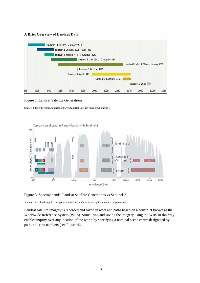
Landsat 4, 5, and 7 images consist of seven spectral bands with a spatial resolution of 30 by 30 m for
Bands 1 to 5 and 7. The spatial resolution for Band 6 (thermal infrared) is 120 m, but is subsequently
resampled to 30m pixels to align with the other 5 bands. Figure 2 shows the operational time windows
of the various Landsat satellite generations.
Landsat 8 is now the preferred satellite from the Landsat series as it is significantly more sensitive, has
additional spectral bands, and is very well calibrated. The previous Landsat series images should only
be used for archival analysis to detect change over time or frequency of events (see the Water
Observations from Space Flood frequency web mapping facility by GeoScience Australia
http://www.ga.gov.au/scientific-topics/hazards/flood/wofs).
The Sentinel-2 satellites will become increasingly relevant as the data becomes increasingly globally
available.
13
A Brief Overview of Landsat Data
Figure 2: Landsat Satellite Generations
Source: https://directory.eoportal.org/web/eoportal/satellite-missions/l/landsat-7
Figure 3: Spectral bands: Landsat Satellite Generations vs Sentinel-2
Source : http://landsat.gsfc.nasa.gov/sentinel-2a-launches-our-compliments-our-complements/
Landsat satellite imagery is recorded and saved in rows and paths based on a construct known as the
Worldwide Reference System (WRS). Structuring and saving the imagery using the WRS in this way
enables inquiry over any location of the world by specifying a nominal scene centre designated by
paths and row numbers (see Figure 4).

14
Figure 4: Worldwide Reference System
Source: http://landsat.gsfc.nasa.gov/the-worldwide-reference-system/
The Landsat 1-3 WRS-1 notation assigns sequential path numbers from east to west to 251 nominal
satellite orbital tracks, starting with number 001 for the first track which crosses the equator at 65.48
degrees west longitude. A specific orbital track can vary due to drift and other factors; thus, a path line
is only approximate. The orbit is periodically adjusted after a specified amount of drift has occurred in
order to bring the satellite back to an orbit that is nearly coincident with the initial orbit. An example
for an area of Melbourne, Australia,
showing path/row grids is shown in
Figure 5.

15
Figure 5: Path and Row Satellite Grids for a Selected Area of Melbourne, Australia.
Landsat 8 and Landsat 7 follow the WRS-2, as did Landsat 5 and Landsat 4, whereas Landsat 1, Landsat
2, and Landsat 3 followed WRS-1.
The Landsat 4, 5, and 7 Worldwide Reference System-2 (WRS-2) is an extension of the global Landsat
1 through 3 WRS-1 and utilises an orderly Path/Row system in a similar fashion. There are, however,
major differences in repeat cycles, coverage, swathing patterns and Path/Row designators due to the
large orbital differences of Landsats 4 and 5 compared to Landsats 1 through 3.
Once the satellite data is pre-processed into Analysis Ready Data this file system is removed and
replaced by each pixel of each image being placed in a spatio-temporal database from which any slice
of data through time and space can be selected.
GEO satellites are located above the equator at an altitude of about 36,000km where they can stay
exactly positioned over the same spot on earth. Originally designed for meteorological use they are
becoming so sophisticated that the sensors are also useful for non-meteorological purposes. The current
highest spatial resolution is 500 m with images taken at 10 minute intervals from the HIMAWARI-8
Satellite, the first of a series of similar satellites (GOES-R Type) that will cover most of the world.
Himawari-8 is positioned over Indonesia and covers half the globe, although at larger off nadir (=off
vertical) angles the satellite creates increasingly skewed pixels.
Figure 6: Visual representation of satellite orbits
Source: http://www.idirect.net/Company/Resource-Center/~/media/Files/Corporate/iDirect%20Satellite%20Basics.pdf
The MEO (Medium Earth Orbit, approximately 20,000 km) satellites are mainly focused on navigation,
communication, and geodetic/space environment science, with an orbit time of 12 hours to 2 hours. For
more information, please visit NASA (National Aeronautics and Space Administration) website:
http://earthobservatory.nasa.gov/Features/OrbitsCatalog/

16
2.3 Active and passive sensors
Figure 7: Active/Passive sensors characteristics
Source: http://lms.seos-project.eu/learning_modules/marinepollution/marinepollution-c01-s02-p01.html.
Wavelengths and frequencies of electromagnetic waves are on logarithmic scales. Passive instruments
detect signals which are naturally available, e.g. sun irradiance reflected or thermal radiation emitted
from a target. Active instruments provide their own source of radiation for target illumination and
returned signal detection.
It is also important to discriminate the electromagnetic wavelength domain these sensors record and
whether they measure reflected sun energy, emissions from the earth (the passive earth observing
sensors) or a signal they emit and then record as it is reflected by the earth (the active sensors).
For the passive sensors wavelengths measured vary from those the human eye can see such as the blue
to green to yellow to orange to red wavelengths (the visible or VIS Wavelengths); the NIR (Nearby
Infrared) wavelengths, the SWIR (Shortwave Infrared Wavelengths), MIR (Mid Infrared Wavelengths
in research mode currently), the TIR (Thermal Infrared Wavelengths) measuring temperature emission
through to the microwave region (or radar). The VIS to NIR to SWIR to MIR sensors operate mainly
during the day time (with some exceptions such as using night time lights to detect marine (shipping &
energy resource platforms) or terrestrial artificial light sources. The TIR and passive microwave sensors
can also detect emissions at night. Passive microwave may be used to estimate soil moisture on land or
ocean salinity.
A separate, recent development is the detection of gravity anomalies using satellites. These anomalies
over time can infer the depletion or recharge of large subsurface groundwater reservoirs as an example.
The active sensors either emit light by lasers in the VIS to NIR domain (LiDAR:Light Detection And
Ranging) or emit microwave energy by synthetic aperture radar (SAR). These systems can work day
and night as they have their own source of electromagnetic energy. LiDAR is used for accurate
estimations of elevation and canopy height or in shallow waters for the bottom depth (bathymetry).
Research and development on LiDAR is focusing on being able to discriminate aspects of the canopy
or of the water column.
SAR is used for imaging the radar backscatter signal from which land cover, flood cover, agricultural
crops, forests etc., illegal & unreported vessels can be detected and measured. SAR interferometry can

17
detect millimetre shifts, such as shifts in resource extraction areas (subsidence) or volcanic or
earthquake regions.
2.4 Applications of algorithms to EO
EO is generally used to determine the spatial distribution of a variable (what’s where?) and to determine
the nature of the variable. For example, colour, depth, fluxes, vigour, concentration, density, mass, etc.
By adding the temporal aspect of repeat coverage the question of state, condition and trend can then be
answered. Therefore, these measured reflections or emissions need to be translated into meaningful
information, such as for official statistics, through the application of algorithms. In general these
algorithms are mathematical equations, statistical or biophysical, geophysical, chemo physical methods
or any combination of these approaches.
The nature of these algorithms has a significant consequence for their use in producing official statistics.
It is possible to discriminate five broad categories with many possible permutations; the first three are
pixel-based methods and the fourth uses this information as well as spatial and contextual information.
In the fifth method hybrid approaches are described.
1. Empirical methods: where a statistical relationship is established between the spectral bands
or frequencies used and the variable measured (field-based) without there necessarily being a
causal relationship. This method is the least suitable for automation across large areas and
varying conditions (sun angle, season, latitude, slope and aspect of terrain, atmospheric
conditions) unless accompanied by a significant, ongoing field measurement activity,
preferably with each satellite overpass.
2. Semi-empirical methods: where a causal relationship is established between the spectral bands
or frequencies used and the variable assessed. This method is less prone to providing spurious
results, although results may have significantly increased error outside the field-based range.
This method has medium suitability for automation across large areas and has less stringent
requirements for frequent field based sampling.
3. Physics-based inversion methods: which are also known as semi-analytical inversion
methods. All required variables are assessed in one spectral inversion simultaneously. This
method provides physics-based consistency in results, and is most suitable for automation
across large areas, provided the inversion model is properly parameterised for the desired
variables. These are also called biophysical, biogeochemical or geophysical inversion methods.
4. Object based image analysis method (OBIA): This method combines spatial, pattern, texture
and spectral information together (e.g. through initial image segmentation) with contextual
information supervised by a human operator. This method has suitability for automation across
the natural or manmade system for which it was developed and is being increasingly used.
5. Artificial intelligence and machine learning methods: these are intelligent, high-dimensional
statistical (often non-linear) models for identifying highly complex relationships in data.
Depending on how these methods are trained (using field measurements or physics-based
models), they cross the realms of empirical to semi-empirical to physics-based and OBIA based
inversion methods.
Methodological approaches to working with EO data are further discussed in depth in Chapter 3.

18
When the physical processes are well understood, we can develop physics-based inversion models.
Often prefixes will be used such as bio-physical or geo-physical etc., indicating the nature of the
variable being sensed. Sometimes EO data can provide useful inputs to such physical models, and this
is the ideal situation. Inverting physical models is only one way of using them. For example, fractional
cover or Leaf Area Index (LAI) can be used in a biophysical model in a forward manner – to predict,
for example, gross primary productivity or evapotranspiration. Another example is water quality; some
aspects of which can be determined from space using physics based inversion models. The advantage
of these inversion models is that once properly parameterised they no longer need in situ data and thus
are a prime candidate for automation of processing of large EO data volumes. Therefore, if it is possible,
the physics based forward and inverse approaches are recommended as they decrease the need for in
situ data and increase the opportunity to be automated.
However, often EO can’t provide direct measures of the inputs, and that is when semi-empirical
methods that find correlations between an EO derived variable and some real biophysical variable are
required. When the physical processes aren’t well understood (e.g. ecology), we can’t use physical
models and resort to empirical, semi-empirical or OBIA or machine learning models, which rely on
statistics to define the relationships rather than physics. In this case, the empirical relationships need to
be continually checked (field work or simulations) to ensure they are not changing across space and
especially through time.
2.5 Combining data: data-data, data-model and model-data assimilation
Increasingly use is being made of combining the information of two or more EO sensors in order to
counteract the disadvantages of some EO sources. This is called data-data fusion or blending. An
example of this approach is using land reflectance in the VIS and NIR coupled with TIR imagery, or
using sensors with high repeat frequency and low spatial resolution with low frequency and high spatial
resolution to compensate for each other’s weakness.
It is also possible to merge EO information with an underpinning model of the phenomenon under
study. This approach is called data-model fusion.
When EO and/or field observation data is used to improve the performance of a model and the model
output is then used to strengthen the validity or accuracy of the field data or EO products or vice versa
in ways that maintain consistency amongst system variables, is cognisant of model and observation
uncertainty, and enhances information value of generated outputs is called model-data assimilation.
2.6 Current examples of EO data applications
Many applications of EO derived geospatial information exist across domains, including but not limited
to the following; biosecurity, biodiversity, forestry, agriculture, soil moisture, catchment water balance,
land atmosphere energy exchange, digital elevation models, minerals, mine site environmental
management, urbanisation, infrastructure, commodity stockpiles, environmental pollution, water
quantity and quality, seagrasses and coral reefs, shallow water bathymetry, coastal and ocean water
productivity, algal blooms, sea state, currents, upwelling and down welling zones, atmospheric air
quality, emergency management and mitigation, disaster risk management, environmental accounting
(i.e. monitoring land cover changes). Many more applications will be developed as sensors become
more sophisticated, and the EO data become more accessible (see section 2.8 on Analysis Ready Data
(ARD).

19
Figure 8: Remote sensing basics: wavelengths and reflectance signatures
Source: http://www.geog.ucsb.edu/~jeff/115a/remote_sensing/remotesensing.html
2.7 CEOS and GEO: international EO organisations
The GEO (Group on Earth Observations) and CEOS (Committee on Earth Observation Satellites) are
two key players related to EO;these two global organisations work closely on various subjects linked
to EO data, and CEOS is often called the “space” arm of GEO. The 2030 Agenda to implement and
monitor the UN SDGs is a great opportunity to reflect the collaboration between the two entities, already
working on a GEO initiative, called EO4SDGs, dedicated to the UN SDGs.
The EO enabling space agencies (through CEOS) and GEO acknowledge they have yet to fully address
the major barriers faced by potential users of EO derived information. The translation of the signal
measured in space to a meaningful variable requires this signal to pass several pre-processing steps until
a signal is calculated, from which (in the case of VIS, NIR or TIR) effects of sensor noise, the
atmosphere, the sun angle, terrain angle, clouds and cloud shadows, canopy shadowing or in the case
of water sun and sky glint reflectance are removed.
CEOS was created in 1984, with an original function to coordinate and harmonise EO to make it easier
for the user community to access and use data. CEOS initially focused on interoperability, common
data formats, the inter-calibration of instruments, and common validation and inter-comparison of
products. However, over time, the circumstances surrounding the collection and use of space-based EO
have changed. Over the past three decades, CEOS has significantly contributed to the advancement of
space-based Earth Observation community efforts. CEOS Agencies, (31 members) communicate,
collaborate, and exchange information on EO activities, spurring useful partnerships such as the
Integrated Global Observing Strategy (IGOS). A full list of CEOS members is available at
http://ceos.org/about-ceos/agencies/.
CEOS played an influential role in the establishment and ongoing development of GEO and the GEOSS
(Global Earth Observation System of System). CEOS Agencies work together to launch multi-agency
collaborative missions and such cooperative efforts has highly benefited users all around the world.
CEOS also provides an established means of communicating with external organisations, enabling
CEOS to understand and act upon these organisations’ EO needs and requirements.

20
Established in 2005, GEO is a voluntary partnership of governments and organisations that envisions
“a future wherein decisions and actions for the benefit of humankind are informed by coordinated,
comprehensive and sustained Earth observations and information.”
See https://www.earthobservations.org/vision.php
GEO has created an initiative ( “EO4SDGs”, Earth Observations in Service of the 2030 Agenda for
Sustainable Development), to organise and realise the potential of EO sources to advance the 2030
Agenda and enable societal benefits through achievement of the SDGs. EO4SDGS especially works to
expand GEO’s current partnerships, enhance its strong relationship with the UN, and foster consolidated
engagement of the individual Member countries and Participating Organisations. CEOS is highly
supporting this GEO initiative, and has also created an ad hoc team on SDGs
(http://ceos.org/ourwork/ad-hoc-teams/sustainable-development-goals/) to better coordinate CEOS
Agencies’ activities around SDGs.
GEO is working closely with key UN entities includes the UN Statistics Division, the United Nations
Committee of Experts on Global Geospatial Information Management (UN GGIM), the UN Sustainable
Development Solutions Network (UN SDSN). Additional potential partners include development
banks, Non-governmental organisations (NGOs), and international entities. Engagement and
partnerships with these entities help build processes, mechanisms and human capacity to include EO
data in national development plans and integrate them with national statistical accounts to improve the
measuring, monitoring and achievement of the SDGs.
One of the actions of the EO4SDGs consists of Capacity Building and Engagement; support to countries
in the implementation of all appropriate measures to properly address the 2030 Agenda. Drawing on
capacity building activities within GEO, this action coordinates and fosters capacity building efforts at
appropriate levels on effective ways to convey methods, enable data access, and sustain use of EO in
the context of SDGs. Activities here draws on and support GEO efforts to characterise user needs.
Given the basis of the SDGs in statistical data, this action includes engagement with the SDG statistical
community about EO as well as capacity building within GEO and the EO community about SDG
statistical principles and practices.
GEO and CEOS will therefore be fully engaged in the process of implementing the UN SDGs,
especially when showing where EO can be useful to monitor some key indicators or to help achieve the
goals/targets.
Some projects or initiatives are already crucial for EO monitoring and their continuity will help better
connecting EO and official statistics worlds. For example, see 2.14.2 the example of GFOI (Global
Forest Observations Initiative), a GEO initiative.
It is recommended for the National Statistical Offices in countries that are members of GEO to establish
a working relationship with their national space/meteorological/science agencies in this area of using
EO data for official statistics.
2.8 Introduction to EO based Analysis Ready Data (ARD)
Many satellite data users, particularly those in developing countries, lack the expertise, infrastructure
and internet bandwidth to efficiently and effectively access, prepare, process, and utilise the growing

21
volume of raw space-based data for local, regional, and national decision-making2. Where such
expertise does exist, data preparation is often limited to a small number of specialists, which limits the
number of end-users of EO data and/or use a diversity of techniques making it difficult for observations
and derived products to be appropriately compared. This results in often inconsistent and sometimes
conflicting results. This is a major barrier to successful utilisation of space-based data, and the success
of major global and regional initiatives that are supported by CEOS3 and GEO.
Therefore, it is useful to introduce the concept of “Analysis Ready Data” (ARD). EO data needs to be
corrected for many effects caused by the distance from the subject being measured and all the
transmission effects as the signal passes from the earth’s surface and is measured in space. Some of
these effects are due to the atmosphere, the solar angle, the viewing angle from the sensor to the target
etc. Pre-processing the data to correct for these effects creates EO data as if the sensor is collecting data
within a few meters of the surface.
This pre-processing of EO data can be automated, thereby reducing the burden on the geospatial and
information experts that are focused on extracting valuable information from this data. Moreover, if
ARD is well defined and preferably peer reviewed, the user of the data can be confident they are
working with data that has an acceptably high level of validity and accuracy.
CEOS has begun to consider the following interim definition:
“Analysis Ready Data (ARD)” are satellite data that have been processed to a minimum set of
requirements and organized into a form that allows immediate value-adding and analysis without
additional user effort”.
Once raw data is processed to ARD it becomes more accessible and useful to properly harness the
multiple technologies and initiatives behind ‘Big Data’, that allow real-time analysis and data mining
to produce better science. Once the ARD state has been reached the algorithms and methods discussed
previously can be applied and importantly are more likely to be comparable across different groups of
users and sensor configurations. For NSOs to derive indicators for statistical purposes there is a
requirement to bring the pre-processed EO data to a ‘Product’ stage where it has been classified into
more meaningful variables such as a land cover classification. This still requires additional expertise
which may be outside or inside an NSO. Refer to section 2.10 and Lewis et al, 2016 for more
information on ARD.
2.9 Variety of EO sources (in situ, airborne)
To work with EO data, NSOs need to be aware of which sources can be used to monitor relevant
variables for official statistics. Besides the most well-known MODIS and Landsat images, there are
many sources of available satellite imagery data, free or commercial, from different EO satellites,
collecting various measurements about the land and land cover, water and atmosphere. MODIS and
Landsat are the most used satellite data sources due to their early launch (providing relatively long-
term archives) and longevity, leading to a significant amount of peer reviewed publications, spatial
resolution coupled with open and free data policies.
However, the two MODIS satellites, originally intended as research instruments, will not be replaced
by identical systems but by an intermediate current system called SUOMI-VIRRS to be followed up
2 NASA useful page to get information on how to use data: https://earthdata.nasa.gov/earth-observation-data/tools
3 From CEOS Draft discussion paper on Analysis Ready Data (CEOS Systems Engineering Office 2016)

22
by the NPOESS sensors that combine meteorological and climate and land and ocean observations.
The Landsat capacity for multispectral 30 m resolution data is no longer the highest spatial resolution
freely available data and is no longer considered state-of-the-art in sensor development, although
Landsat 8 is a significant improvement over the Landsat 5 and 7 satellites.
Below is a guide to selecting the best spectral bands to use for Landsat 8.
Band Wavelength Useful for mapping
Band 1 – coastal
aerosol 0.43 - 0.45 Coastal and aerosol studies.
Band 2 – blue 0.45 - 0.51 Bathymetric mapping, distinguishing soil from vegetation
and deciduous from coniferous vegetation.
Band 3 - green 0.53 - 0.59 Emphasises peak vegetation, which is useful for assessing
plant vigour. Total suspended matter in water bodies.
Band 4 - red 0.64 - 0.67
Discriminates vegetation spectral slopes; also measures the
primary photosynthetic pigment in plants (terrestrial and
aquatic) : chlorophyll-a.
Band 5 - Near Infrared
(NIR) 0.85-0.88 Emphasises biomass content and shorelines.
Band 6 - Short-wave
Infrared (SWIR) 1 1.57 - 1.65
Discriminates moisture content of soil and vegetation;
penetrates thin clouds
Band 7 - Short-wave
Infrared (SWIR) 2 2.11 - 2.29
Improved moisture content of soil and vegetation and thin
cloud penetration
Band 8 - Panchromatic 0.50 - 0.68 15 meter resolution, sharper image definition
Band 9 – Cirrus 1.36 - 1.38 Improved detection of cirrus cloud contamination
Band 10 – TIRS 1 10.60 – 11.19 100 meter resolution, thermal mapping and estimated soil
moisture
Band 11 – TIRS 2 11.5 - 12.51 100 meter resolution, Improved thermal mapping and
estimated soil moisture
Table 1: Landsat 8 Operational Land Imager (OLI) and Thermal Infrared Sensor (TIRS)
Source: http://landsat.usgs.gov/best_spectral_bands_to_use.php plus modifications by authors (Dekker, A., Held, A., and Kerblat, F.)
The European Commission’s Copernicus Sentinel system of satellites (Sentinel types 1 through 6 now
funded through to 2030, managed by the European Space Agency and EUMETSAT) are state of the art

23
operational systems with significantly enhanced capabilities. Take for example the Sentinel-2 satellite
with 10 m pixels and (with the launch of Sentinel 2B from 2017 onwards) a repeat visit cycle of one
image every five days.
We are now in the early stages of a technology revolution; a global sensing revolution, in which ground-
based, aerial and space-based sensors, and new forms of data analytics, will enable entirely new
approaches to the global administration of our planet. These new geospatial technologies can transform
the accuracy, frequency, transparency and progress on assessing many of the indicators for the SDGs
or other forms of official statistics at a significantly reduced cost per variable per square kilometre.
NSOs and decision-makers will need to take into account this continuous technologic evolution,
including a democratisation of EO satellite use. Going forward, it is recommended that NSOs increase
training of their people in working with these data sources and permanently update these skills as
technologies change.
2.10 Use of ARD or EO sources for official statistics
The advantage of EO data is its large spatial and temporal coverage, and its accessibility, reliability,
and accuracy have improved dramatically. With EO satellite data, almost 100% of the earth surface is
covered repeatedly, far more than could ever be achieved using field based or airborne technologies.
A disadvantage of EO is that contrary to field based, or in-situ measurements, EO estimates are derived
indirectly (although one could argue that all sensor technologies do this including the human eye, which
is effectively a remote sensing system with 3 wavelengths, also called spectral bands). While results of
EO for potential operational use in many areas look promising, in other areas EO has not yet succeeded
in extracting all the required information gaps and opportunities for further development of many
operational applications still exist.
EO data, especially when used jointly with in-situ or model data, can make an essential contribution to
resources management and development. However, it is not always easy to generate a clear picture of
the boundaries between complementarity and substitutability of these techniques. Herein lies the risk
for the common practitioner and planner; it is easy to become overwhelmed by all these advances and
promises, while also feeling constrained by the institutional inability to cope with the long time periods
and significant budgetary resources required for in-situ measurements. To make sound decisions,
practitioners need to be aware of both the potential value and limitations of applications of EO
technology and products, through informed recommendations and the development of practical, result-
oriented tools. See Chapter 5 Figures 32 and 33 for more information.
Collecting, using, analysing and storing Big Data is a challenge that can be at least partially addressed
by using EO satellite sources due to their highly structured nature and being designed for their specific
purpose.
NSOs are currently using traditional data sources (surveys, collection of samples, etc.) which are still
valid and useful, but EO data can help complete or obtain more accurate, frequent, spatially or
temporally extrapolated, or temporally interpolated measurements.
In 2015, the UN Global Working Group on Big Data conducted a survey enquiring about the strategic
vision of NSOs and their practical experience with Big Data. It is interesting to see that among the 93
countries which responded, the statistical offices considered “faster statistics”, “reduction of respondent
burden” and “modernization of the statistical production process” to be the main benefits of using Big
Data. Two other reasons to use Big Data followed; “new products and services” and "cost reduction”.

24
Figure 9: Main benefits of Big Data for NSOs
Source: Figure 5: Global survey analysed in the “Report of the Global Working Group on Big Data for Official Statistics”
EO derived information is a growing opportunity to complement traditional sources (ground or socio-
economic data) when there is a lack of data. Using EO data products can make spatially or temporally
denser data (globally), improve frequency or richness of data, and save money on traditional methods
(surveys methods are highly time-consuming and expensive). EO data can be a game-changer for
monitoring global initiatives (such as the current ones GFOI, GEOGLAM (GEO Global Agriculture
Monitoring), etc.), and therefore would be useful methods to help monitor the UN SDGs by measuring
and collecting some relevant indicators. If the stage of an automated EO processing system is achieved
updates to official statistics could be done more frequently e.g. monthly.
Despite the potential benefits of EO, it is not always the most appropriate source for producing official
statistics. Below are some criteria for practitioners to consider when assessing whether EO data is fit
for their purposes. A further cost benefit analysis process is outlined in Chapter 5.
2.11 Validity and definitions
For empirical, semi-empirical, OBIA, AI and machine learning approaches there are three major sources
of uncertainty in satellite estimations: (i) retrieval errors, (ii) sampling errors, and (iii) inadequate
ground reference observations. In the case of physics-based inversion models (iv) the parameterisation
of the model can introduce uncertainties; however these methods deal better with the first three sources
of uncertainty. A physics-based inversion model does not necessarily need ground observations for
validation once it is parameterised in a representative manner of the variability of the target variables.
This is a bonus in the case of needing to estimate variables in remote areas. Moreover, physics-based
inversion methods can be easily transferred from one EO sensor to another without needing an entire
new set of ground measurements.
Additional sources of uncertainty originate in the need for model calibration, different spatial scales,
and the need for bias correction of the estimated values prior to being used. An important challenge in
the use of remote sensing based estimates is how to reconcile them with ground reference
measurements, as both can be observations of a very different nature. Thus, observations from space
need to be analysed, validated, and used in accordance with their limitations.
0% 10% 20% 30% 40% 50% 60% 70% 80% 90%100%
Faster, more timely statistics
Reduction of respondent burden
Modernization of the satistical production process
New products and services (e.g. Map development,visualizations)
Cost reduction
Meeting new demands such as SDGH indicators
Government Policy on the informaton society
Non-OECD countries
OECD countries

25
Sampling and measurement errors can result from the measurement of a variable in the wrong place
(e.g. rainfall measured at the cloud base instead of at the ground surface) and from indirect estimations
and biases in measurement sensors, entailing errors in the magnitude of the (e.g. precipitation) rate
being measured. These errors will vary with the geographic and atmospheric setting.
However, ground reference measurements also have errors in validity, representativeness,
completeness, and in the case of laboratory analysis also contain errors of sample preparation, material
extraction, storage, and measurement errors. Thus, both EO data and ground reference data are variables
with errors. Essentially these are measurement error models that need to account for errors in the ground
reference variables, often seen as the independent variables. Note that in the case of crop classification,
these cannot be obtained directly from EO data but can be from ground reference data. Although there
will be measurement errors, ground reference data do not require modelling to turn them into the
variables of interest to agricultural statistics, thus avoiding modelling errors.
A useful publication on validity of EO based information products (focusing on hydro meteorological
variable estimation) can be found in: From Earth Observation for Water Resources Management:
Current Use and Future Opportunities for the Water Sector
(https://openknowledge.worldbank.org/bitstream/handle/10986/22952/9781464804755.pdf). Here a
short summary is given, with some additional information as pertaining to physics-based inversion
models.
Despite the uncertainties inherent to in-situ or ground reference measurements, it is believed the
accuracy of an EO data product will rarely be as high as that of an equivalent field measurement at that
location. Nevertheless, despite the generally lower site specific accuracy, EO products should still be
considered an important alternative data source, as EO imagery can provide information with greater
spatial extent, spatial density, and/or temporal frequency than can most field-based (point-based)
observation networks. . Furthermore, EO derived information can be acquired much faster and are more
cost effective than most traditional survey based methods. Once validated, the data can also be readily
extrapolated across large regions and remote areas with high efficacy. It is for these reasons that a
combination of EO and field (ground reference) data generally provides the best information outcomes.
If it is possible to have a model ( e.g. deterministic) that sufficiently describes the phenomenon of
interest then model, EO and field data assimilation is the most powerful way to derive the required
information.
2.12 When is EO considered as “valid”? The fit-for-purpose argument
The most useful definition in the case of trying to establish the validity of an EO based information
product is the concept of it being fit for purpose. An EO scientist will, in general, try to achieve the
highest level of precision, accuracy and validity. For statisticians, in a geospatial analysis context, fit
for purpose for EO derived information will focus around the question: is there an advantage with
respect to existing non-EO based methods? Aspects which may be considered are timeliness, spatial
and temporal coverage, assessing multiple variables from the same dataset, independence of
respondents, avoiding political or other biases etc.
Among NSOs, quality is generally accepted as "fitness for purpose". However, this implies an
assessment of an output, with specific reference to its intended objectives or aims. Quality is therefore
a multidimensional concept which not only includes the accuracy of statistics, but also other aspects
such as relevance and interpretability. Over the last decade, considerable effort has been made to give
a solid framework to these definitions in statistics.

26
For instance, the ABS Data Quality Framework (DQF) 2009 is based on the Statistics Canada Quality
Assurance Framework (2002) and the European Statistics Code of Practice (2005). Besides the
“Institutional environment”, six dimensions have been specifically defined to help getting the best data
quality; Relevance, Timeliness, Accuracy, Coherence, Interpretability, and Accessibility. The following
table presents some thoughts on how these dimensions can be viewed from an EO perspective, and add
two additional definitions from the EO discipline; integrity and utility.
Table 2: Statisticians and EO scientists’ definitions: summary
ABS DQF or
NSOs community
Key aspects (How NSOs
assess the dimension?)
EO/remote sensing community
Institutional
environment
“The institutional
and
organisational
factors which
may have a
significant
influence on the
effectiveness and
credibility of the
agency producing
the statistics”.
• Impartiality and
objectivity
• Professional
independence
• Mandate for data
collection
• Adequacy of
resources
(sufficient to meet
needs)
• Quality
commitment
• Statistical
confidentiality
In principle EO data is impartial, objective and
reproducible. The processing must be transparent
and open to scrutiny.
Space agencies or commercial aerospace
companies provide the raw “Top of Atmosphere”
data. These same agencies and others pre-process
the data to an analysis ready format. Subsequently
the ARD needs to be translated into a relevant
variable either by or for the NSO.
Criteria to look for: comprehensive information
about the EO sensor specifications, its calibration
(pre-flight, on-board and vicarious); does reliable
peer reviewed literature exist? It is essential to have
transparent algorithms and documentation,
complete metadata and product documentation,
open access products, or open access algorithms.
The concept of ARD is important here as it solves
one aspect of institutional capacity: If world-class
experts pre-process the EO data to ARD EO Data
Cubes the institutional capacity can focus on
applying the right algorithm, parameterisation and
validation. It is essential to have geospatial
analytics capacity.
Relevance “How well the
statistical product
or release meets
the needs of users
in terms of the
concept(s)
measured, and
• Scope and
average4
• Reference period5
• Geographic detail
• Main outputs/data
items
Reference period =Record life, i.e. EO mission
life. Could be one satellite sensor or a suite of
sensors such as Landsat (multiple sensors from
1984 onwards).
4 Purpose or aim for collecting the information, including identification of the target population, discussion of whom the data represent, who
is excluded and whether there are any impacts or biases caused by exclusion of particular people, areas or groups
5 Period for which the data were collected, as well as whether there were any exceptions to the collection period
27
ABS DQF or
NSOs community
Key aspects (How NSOs
assess the dimension?)
EO/remote sensing community
the population(s)
represented”.
• Classification and
statistical
standards
• Types of estimates
available
• Other sources6
Geographical detail corresponds to the spatial
resolution of the EO sensor which needs to be
selected for the intended purpose.
Temporal resolution is also important for EO
applications and also varies with sensor.
Main outputs/data items and types of estimates: see
discussion in Chapter 3 on various methods and
algorithms.
Many EO classification methods exist but there is
a need for standards that are widely followed (e.g.
GFOI and GEOGLAM). Potentially NSOs could
develop classification standards for this type of
data.
Types of estimates available will be enhanced by
increases in: geographic coverage (global mapper,
regional, on demand) and sensor resolution
considerations; spatial, spectral, temporal,
radiometric.
Other sources: an issue to consider is whether
there is no, minimal or adequate ground reference
data available.
A related concept in EO is integrity; biophysical
and scientific integrity. This relates to the ability to
relate and interpret EO derived metrics to
biophysical processes.
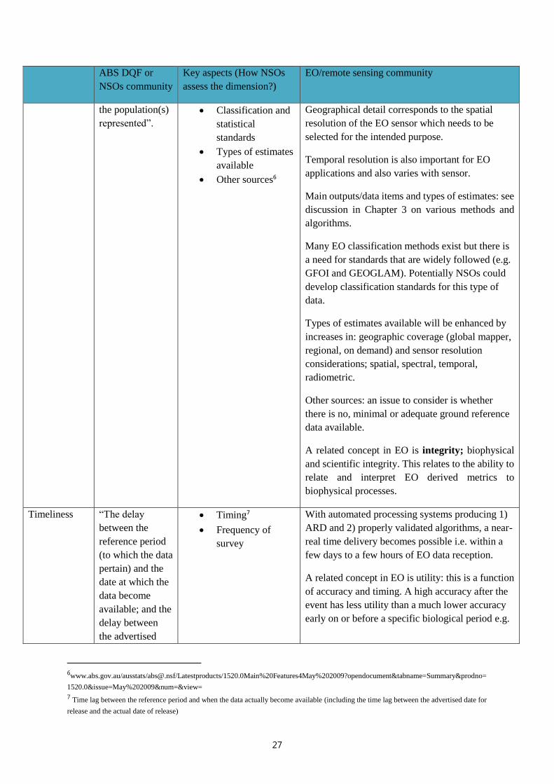
Timeliness “The delay
between the
reference period
(to which the data
pertain) and the
date at which the
data become
available; and the
delay between
the advertised
• Timing7
• Frequency of
survey
With automated processing systems producing 1)
ARD and 2) properly validated algorithms, a near-
real time delivery becomes possible i.e. within a
few days to a few hours of EO data reception.
A related concept in EO is utility: this is a function
of accuracy and timing. A high accuracy after the
event has less utility than a much lower accuracy
early on or before a specific biological period e.g.
6www.abs.gov.au/ausstats/[email protected]/Latestproducts/1520.0Main%20Features4May%202009?opendocument&tabname=Summary&prodno=
1520.0&issue=May%202009&num=&view=
7 Time lag between the reference period and when the data actually become available (including the time lag between the advertised date for
release and the actual date of release)

28
ABS DQF or
NSOs community
Key aspects (How NSOs
assess the dimension?)
EO/remote sensing community
date and the date
at which the data
become
available”.
sowing, flowering of crop or harvesting or e.g. in
the case of coral reefs, a bleaching event.
Accuracy “The degree to
which the data
correctly describe
the phenomenon
they were
designed to
measure”.
“Should be
assessed in terms
of the major
sources of errors
that potentially
cause
inaccuracy”.
• Coverage error
• Sample error
• Non-response
error
• Responses error
• Other sources8
For EO derived information products the validity
has to be established first. Thus, it essential to
establish a causal relationship between the EO
measurement and the phenomenon. Empirical
algorithms can run the risk of producing spurious
results.
EO data have a high spatial and temporal coverage
but can have data gaps due to low repeat visits and
/or inclement weather or other image conditions.
For classification results (products with categorical
variables, e.g., land use land cover, vegetation type,
benthic type), the users, producers and overall
accuracy need to be determined. Note that Kappa
statistic is considered defunct.
For products with continuous variables (e.g.
fractional cover, chl-a concentration), there are
numerous statistics used. Common statistics
include RMSE and variants thereof, bias, R2,
Pearson’s R.
For RMSE and bias, the results can vary
significantly based on which value is put first; EO
or ground reference. R2 and R obfuscate how well
the data match up (things can be highly linearly
correlated and not fall along the one-to-one line).
It is essential to assess EO products with
independent data. Best practice is all accuracy
assessment done with independent data. Note
though, that ground reference measurements also
contain uncertainties.
Coherence “The internal
consistency of a
statistical
collection,
Changes to data items
Comparison across data
items
EO data sets are internally very consistent as they
are all based on measurements by the same
instrument. However the processing from raw top
of atmosphere data to ARD continuously
8http://www.abs.gov.au/ausstats/[email protected]/Latestproducts/1520.0Main%20Features6May%202009?opendocument&tabname=Summary&pr
odno=1520.0&issue=May%202009&num=&view=

29
ABS DQF or
NSOs community
Key aspects (How NSOs
assess the dimension?)
EO/remote sensing community
product or
release, as well as
its comparability
with other
sources of
information,
within a broad
analytical
framework and
over time”.
Comparison with previous
releases
Comparison with other
products available
improves. Similarly, the EO algorithms improve
continuously. The increased use of EO data,
ground reference data and model data improves
validity and accuracy but may make comparison
with previous version derived data more complex.
The coherence issue also occurs when multiple
sources of EO data are used.
Interpretabilit
y
“The availability
of information to
help provide
insight into the
data”.9
Presentation of the
information
Availability of information
regarding the data
The interpretation of EO data derived information
requires several skills in the EO processing domain
as well as the geospatial analytics domain. EO data
is often reduced to table and graphics destroying
some of the interesting spatial and temporal
contextual information. Good documentation and
record keeping is key. A guide on what the scope
and limitations are of using EO data is required.
Accessibility
“The ease of
access to data by
users, including
the ease with
which the
existence of
information can
be ascertained, as
well as the
suitability of the
form or medium
through which
information can
be accessed”.
“The cost of the
information may
Accessibility to the public
(extent to which the data
are publicly available, or
the level of access
restrictions)
Data products available10
EO data products are typically very large and
complex, which challenges accessibility. EO data
products need to be accessible, meaning they need
to be delivered in data formats that are
standardised and easily openable by a variety of
different software, especially open access
software. It is also preferred that data products be
open access (GEO). It is useful if the EO data is
supplied according to open geospatial standards
(OGS) and open source geospatial software and
data (OSGeo) standards.
Another standardisation is through the Geospatial
Data Abstraction Library (GDAL) which is a
computer software library for reading and writing
raster and vector geospatial data formats.
There is a joint standards working group of the
OGC and the W3C that is developing an approach
9 Information to assist interpretation may include the variables used, the availability of metadata, including concepts, classifications, and
measures of accuracy. 10 specific products available (e.g., publications, spreadsheets), the formats of these products, their cost, and the available data items which
they contain

30
ABS DQF or
NSOs community
Key aspects (How NSOs
assess the dimension?)
EO/remote sensing community
also represent an
aspect of
accessibility for
some users”.
to publishing EO data as “linked data” for easy
access, employing a model for Data Cubes that
was originally developed by the statistical SDMX
community.
If ARD is adopted by all prior to the translation of
this ARD data to a meaningful information
product the interpretability will increase as a
growing body of knowledge is more easily
created. This will also lead to more standardised
products.
As EO use by NSOs is relatively new, pilot and demonstration studies that explore these definitions and
refine the table above are recommended. Some pilot studies conducted by members of the UN Satellite
Imagery and Geospatial Data Task Team are described in Chapter 4.
In the following section, it will be shown the potential of using EO satellite data is much more than
using only time series of MODIS or LANDSAT images. More sources are available, and examples will
be presented about which sensors are most suited to get the best expected data quality
2.13 Earth Observation data information sources available
Figure 10: Operational weather satellites
Source: CEOS EO Handbook: http://www.eohandbook.com/eohb2011/climate_satellites.html

31
A comprehensive list of EO satellites past, present and future exists on the online WMO Oscar database
that contains 645 entries (per April 2016). https://www.wmo-sat.info/oscar/satellites
Filters exist for sorting the data on:
1. Acronym of earth observing sensor platform (that may contain multiple payloads: a single
payload is the specific earth observing sensor),
2. Launch date and end-of-life;
3. Space agency programme name,
4. List of orbital characteristics and
5. Payload
As an example, look at Sentinel-3 (an important sensor for the next 15 years for land and ocean visible
and nearby infrared monitoring; as well as land and ocean surface temperature measurement and with
a land and ocean altimeter).
There are two Sentinel-3 A and B satellite platforms in the system; one was launched on 16th February
2016 and one will be launched in 2017. After that Sentinel-3 C and D are already funded and will be
similar replacing Sentinel-3 A and B. Sentinel E and F are also planned but will be amenable to
enhanced sensor performance based on the results of the preceding 4 satellites. Sentinel-3 A and B both
have an expected lifetime of 7 years. Expected lifetime can be exceeded 3 to 4 fold for some EO sensors-
space agencies are often cautious about this aspect. It flies in a sun-synchronous orbit, meaning it will
pass exactly over the same strip of earth at the same solar time, at 814.5 km altitude. Its status is
operational for Sentinel 3 A and Planned for Sentinel 3 B. The payload is composed of 7 sensors:
DORIS, GPS, LRR, MWR, OLCI, SLSTR and SRAL. The first four sensors are mainly used for exact
positioning and assessment of atmospheric conditions, whereas the last three are the actual earth
observing sensors with an application to detecting and monitoring the earth; OLCI (Ocean Land Colour
Imager), SLSTR (Sea and Land Surface Temperature Radiometer) and SLAR (Synthetic Aperture
Radar Altimeter).
On the WMO Oscar database, by selecting the EO sensor acronym one is transferred to the instrument
page where a wealth of information on the sensor is presented. Information is also presented on other
satellites this instrument also flies on; its contribution to Space Capabilities and a very informative
“Tentative Evaluation of Measurements” containing a list of measurements that can typically be
retrieved from this type of instrument. For OLCI this table is as follows below11.
Variable Relevance for
measuring
this Variable
Operational
Limitations
Processing maturity
Ocean Diffuse Attenuation
Coefficient (DAC)
1-primary Clouds Consolidated
methodology
11 Source: https://wmo-sat.info/oscar/instruments/view/374: Tentative Evaluation of Measurements .The following list indicates which
measurements can typically be retrieved from this category of instrument. To see a full Gap Analysis by Variable, click on the respective
variable. Note: table can be sorted by clicking on the column headers.

32
Variable Relevance for
measuring
this Variable
Operational
Limitations
Processing maturity
Colour Dissolved Organic Matter
(CDOM)
1-primary Clouds Consolidated
methodology
Ocean chlorophyll concentration 1-primary Clouds Consolidated
methodology
Ocean suspended sediments
concentration
1-primary Clouds Consolidated
methodology
Normalised Difference
Vegetation Index (NDVI)
1-primary Clouds Consolidated
methodology
Oil spill cover 2-very high Clouds Consolidated
methodology
Cloud top height 3-high Clouds Consolidated
methodology
Short-wave cloud reflectance 3-high No specific
limitation
Consolidated
methodology
Aerosol volcanic ash (Total
column)
3-high Clouds Consolidated
methodology
Sea-ice cover 3-high Clouds Consolidated
methodology
Aerosol Optical Depth 3-high Clouds Consolidated
methodology
Cloud optical depth 3-high Cloud not too
dense
Consolidated
methodology
Fraction of Absorbed PAR
(FAPAR)
3-high Clouds
Land use
Consolidated
methodology
Integrated Water Vapour (IWV) 3-high Clouds Consolidated
methodology
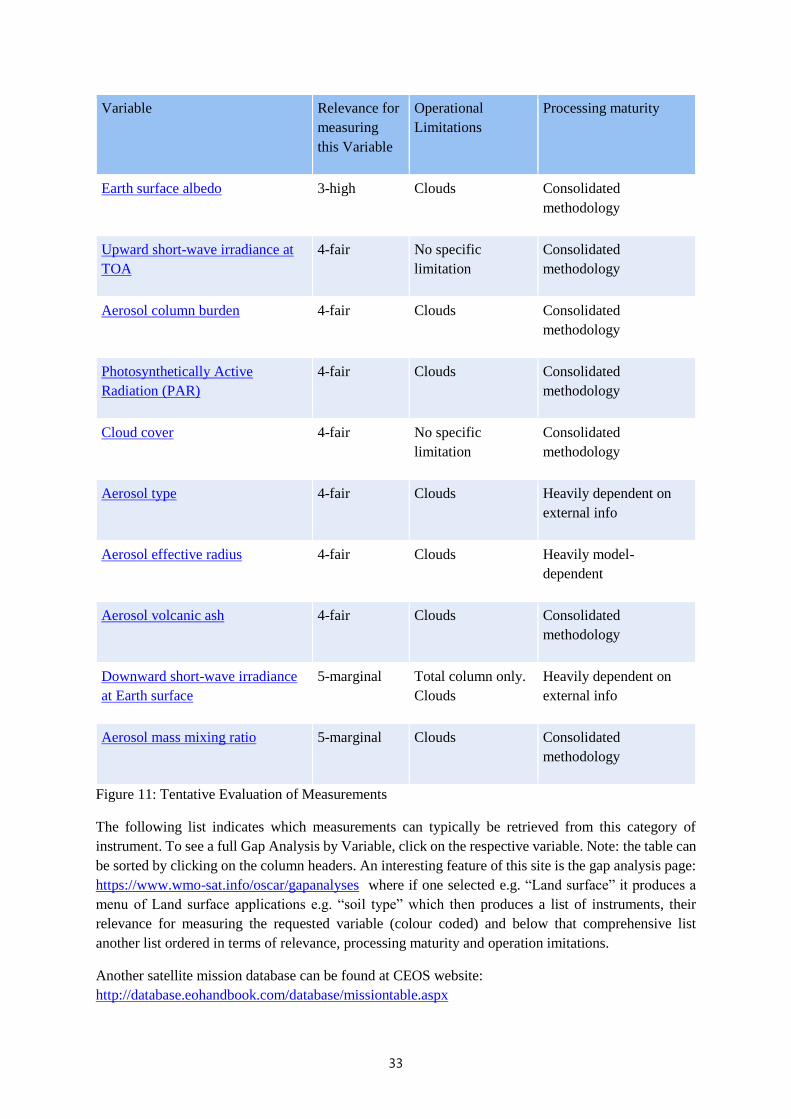
33
Variable Relevance for
measuring
this Variable
Operational
Limitations
Processing maturity
Earth surface albedo 3-high Clouds Consolidated
methodology
Upward short-wave irradiance at
TOA
4-fair No specific
limitation
Consolidated
methodology
Aerosol column burden 4-fair Clouds Consolidated
methodology
Photosynthetically Active
Radiation (PAR)
4-fair Clouds Consolidated
methodology
Cloud cover 4-fair No specific
limitation
Consolidated
methodology
Aerosol type 4-fair Clouds Heavily dependent on
external info
Aerosol effective radius 4-fair Clouds Heavily model-
dependent
Aerosol volcanic ash 4-fair Clouds Consolidated
methodology
Downward short-wave irradiance
at Earth surface
5-marginal Total column only.
Clouds
Heavily dependent on
external info
Aerosol mass mixing ratio 5-marginal Clouds Consolidated
methodology
Figure 11: Tentative Evaluation of Measurements
The following list indicates which measurements can typically be retrieved from this category of
instrument. To see a full Gap Analysis by Variable, click on the respective variable. Note: the table can
be sorted by clicking on the column headers. An interesting feature of this site is the gap analysis page:
https://www.wmo-sat.info/oscar/gapanalyses where if one selected e.g. “Land surface” it produces a
menu of Land surface applications e.g. “soil type” which then produces a list of instruments, their
relevance for measuring the requested variable (colour coded) and below that comprehensive list
another list ordered in terms of relevance, processing maturity and operation imitations.
Another satellite mission database can be found at CEOS website:
http://database.eohandbook.com/database/missiontable.aspx

34
It is organised slightly differently with the mission name being the initial field (equivalent to the earth
observing sensor platform in the Oscar database). Next the responsible space agency or commercial
operator, status, launch date, end of life data , then the applications, followed by the instruments that do
the measurements for these applications and then the orbit details and the URL.
An attractive feature of this database is the ability to search on keywords e.g. “applications” by going
to the page of http://database.eohandbook.com/measurements/overview.aspx
There is a quick informative overview of the measurements split into categories of atmosphere, land,
ocean snow and ice and gravity and magnetic fields. In each category on the right hand a small graph
is visible with timelines and if selected will open a graph showing the full timelines of past, present and
planned sensors allowing an estimation of the continuity of that particular data stream. By selecting e.g.
under “Land” the category “vegetation” a new page opens with all the vegetation variables that can be
measured.
For example if Measurements > Land > Vegetation >Chlorophyll Fluorescence from Vegetation on
Land is selected an earth observing instrument overview is presented with a concise summary of the
intended applications and showing the planned instruments that are intended for carbon estimation by
measuring solar induced chlorophyll fluorescence.
The following is a list of several satellite imagery repositories where data can be downloaded for free.
• USGS Earth Explorer;
• ESA Sentinel Mission;
• NOAA CLASS;
• NASA Reverb;
• Earth Observation Link(EOLi);
• National Institute for Space Research (INPE), specific to South America and Africa; Bhuvan
Indian Geo-Platform of ISRO;
• JAXAs Global ALOS 3D World;
• NOAA Data Access Viewer Discover Authoritative Datasets;
• VITO Vision Coarse Vegetation Data;
• NOAA Digital Coast Snorkel the Seashore;
• Global Land Cover Facility Derived Satellite Data
• DigitalGlobe Free Product Samples;
• BlackBridge/Geo-Airbus Tag Team Champions of Satellite Imagery;
• UNAVCO Research Data.
The USGS Earth Explorer is one of the most famous and popular agencies for freely available Landsat
data. Users are required to register in order to access the USGS data repository and this registration is
free of charge.
For detailed information on suitable EO sensors past, present and future for water resources see the
open report written for World Bank12. It provides an overview of the issue areas related to water
resources management, and discusses the data requirements for addressing these issues, focusing on
12 García, Luis E., Diego J. Rodríguez, Marcus Wijnen, and Inge Pakulski, eds. Earth Observation for Water Resources Management:
Current Use and Future Opportunities for the Water Sector.Washington, DC: World Bank Group.doi:10.1596/978-1-4648-0475-5. License:
Creative Commons Attribution CC BY 3.0 IGO

35
those variables that can be obtained or estimated through EO. Besides the surface characteristics, such
as topography, land subsidence, and others, Earth observation can address eight key hydro
meteorological variables relevant to water resource management applications; precipitation,
evapotranspiration, soil moisture, vegetation, land use, and land cover; groundwater, surface water,
snow and ice, and water quality.
2.14 Data product characteristics
Types of Data Obtained from EO (example of Water management)
Data type Description
Raw data Sensor measurements as received directly from the satellite, formatted as
“digital counts.”
Processed data
a) TOA (Top-of-atmosphere) signal.
Raw data processed to TOA data: conversion to real-world units, such as
radiance (W m-2 nm-1 sr-1) or reflectance (%); signal calibration.
b) Surface signal.
TOA data processed to surface-equivalent data: corrections applied to remove
atmospheric and solar-sensor viewing-angle effects; scene stitching;
geolocation and re-projection.
Data products
Conversion of processed data into products that describe real-world (usually
biophysical) variables such as chlorophyll concentration, leaf area, rainfall
rate, surface temperature, and soil moisture mass.
Information
products
Conversion of data products into management-relevant information for
decision support, for example, eutrophication state of a lake, flood risk of a
river delta, and sustainable irrigation rates in an agriculture area.
2.14.1 Key characteristics of data products
Spatial Resolution (sensor-specific)
The spatial resolution of EO data, sometimes called the spatial frequency or image resolution, refers to
the pixel size of an image. The spatial resolution of data determines the precision with which the spatial
variation of the observed phenomenon can be captured. A relatively large pixel size will capture less
fine-scale spatial variation than a relatively small pixel size. Thus spatial resolution is defined as the
size of the smallest individual component or dot (called a pixel) from which the image is constituted.
For instance, if a satellite's resolution is stated as "5 meters," each pixel in the imagery has a size of 5
meters by 5 meters.

36
The other aspect is the swath of a sensor; this is equivalent to the number of pixels across that track
direction of the satellite. E.g. if an instrument has 1000 pixels of 5 m its swath width is 5 km. If a
satellite sensor has 2000 pixels of 1 km then the swath width is 2000 km. A larger swath width is
associated with a higher repeat coverage rate for one sensor on one satellite. By having multiple
satellites the coverage rate increases with each sensor on each satellite.
When a pixel straddles two (or more) distinct ground features (such as a water body and adjacent
vegetation), the pixel captures a mixture of the signals from both features, and is sometimes referred
to as a “mixel”. Mixels make image interpretation more difficult and, the larger the pixel size, the
more mixels the data are likely to contain. Mixed pixels are further described in Chapter 3.
Temporal frequency (sensor-specific)
The temporal frequency of data (or the temporal resolution) refers to how often a sensor makes
observations of a given location. In the case of polar-orbiting satellites, frequency is related to overpass
frequency and is typically measured in days. With the current constellations for LEOs sub day capacity
can be achieved in some cases. The frequency of imagery by geostationary satellites is much higher,
being measured in the order of minutes to hours as the sensor is stationary above a fixed location above
the equator The distance of geostationary sensors to the earth (~ 36000 km) means the spatial resolution
is low( currently between 05. And 2 km). Relatively high-frequency observations are better able to
capture the dynamics in fast-changing processes than are relatively low-temporal frequency
observations.
For some applications, the time of observation can be important, either to ensure the observations occur
at the same time each day, or because observations need to occur at specific times of the day.
Record length (sensor-specific)
The record length refers to how long the record of data is. This is typically a function of the period of
operation of the satellite (or series of similar satellites), and so is determined by the mission launch and
end dates. Often, however, satellite sensors acquire data long past their planned mission end dates (e.g.
Landsat-5).
Generally speaking, the longer the record length, the older the satellite and its associated technology.
Thus, there is usually a trade-off between record length and other data attributes such as accuracy,
spatial resolution, and/or number of spectral bands. On the other hand long lasting sensor systems and
their data streams have often created a significant opportunity for developing operational information
extraction methods, supported by relevant scientific and applied literature.
Field or ground reference data requirement (product-specific)
Some EO data products are generated solely from satellite observations, some from a combination of
satellite and field-based observations. The latter have much higher input data requirements, and so are
more dependent on the availability of suitable field data. Traditional survey data captured by NSOs may
offer suitable field validation data in some cases. EO data generated from a combination of satellite and
field based observations are also generally more complex to generate and can become limited to the
specific locations and times the field data represent.
• Low field-based data requirement products refer to data products that do not use field data, or
use them only for initial parameterisation of algorithm or for algorithm output validation
purposes;

37
• Medium field-based data requirement products refer to data products that need field data for
calibration of the EO data, or use a moderate amount of field data in the derivation of the final
EO product itself (such as when river gauge data are combined with satellite-derived flood
extent data to estimate flood volumes);
• High field-based data requirement products refer to data products that incorporate multiple
sources of field data (e.g. most evapotranspiration (ET) and soil moisture data products),
sometimes in complex data assimilation systems.
Data product source reliability (product-specific)
Data product reliability refers to the certainty of supply of that product across space and through time.
The greater the spatial coverage, the more frequently the product is updated; the greater the number of
options for sourcing the product, the higher the reliability of the product.
• Low reliability describes a product that is tailor-made for a specific time, region, or application,
or is generated by only one organisation;
• Medium reliability describes a product that typically has wide (global) coverage and is
frequently updated but is provided by just one source organisation;
• High reliability describes a product with global coverage that is frequently updated and can be
sourced from multiple, independent organisations.
Data product accuracy (product-specific)
The accuracy of data products is an estimation of the uncertainty associated with the data estimates.
Accuracy can be described in absolute terms (that is, in physical units such as mm/y) or in relative terms
(usually as a percentage). So, for example, if an estimate of evaporation of 200 mm/y has an error of 10
percent (and thus an accuracy of 90 percent), the real value is likely to be between 180 and 220 mm/y
but may be lower than 180 or higher than 220 mm/y.
Please note: rarely will the accuracy of an EO data product be as high as that of an equivalent field
measurement at that precise location (although this has not been systematically analysed often enough).
Although when extrapolating field measurement results through time and space EO observations are
likely to become more accurate overall.
The field of quality assurance for EO is in rapid development and standards are being developed. We
refer to the GEO activity on “A Quality Assurance Framework for Earth Observation: Principles”
(http://wiki.esipfed.org/index.php/Data_Understanding_-_Quality_(ISO-19157) as well as ISO
19157:2013 - Geographic information -- Data quality for detailed information.
In Yang et al (2013) a relevant summary is presented on data quality in earth observation. Fig (below)
describes essential aspects of EO data quality assessment

38
Figure 12
The Yang paper addresses the following quality aspects known from ISO standards, which might be
characterised as producer data quality elements because they are known by the data producer:
• completeness: presence and absence of features, their attributes and relationships;
• logical consistency: degree of adherence to logical rules of data structure, attribution and
• relationships;
• positional accuracy: accuracy of the position of features;
• temporal accuracy: accuracy of the temporal attributes and temporal relationships of features;
• thematic accuracy: accuracy of quantitative attributes and the correctness of non-quantitative
• attributes and of the classifications of features and their relationships; and
• lineage: information about the provenance of the dataset, including details of processing
applied.
In addition, Yang et al add that good quality metadata records are essential too. An interesting aspect is
that end users also desire ‘soft’ knowledge about data quality—i.e. data providers’ comments on the
overall quality of a dataset, any data errors, potential data use and any other information that can help
to assess fitness-for-use of the data. Finally importance was given to dataset provenance as well as
citation and licensing information when assessing whether data are fit for purpose.
Despite their generally lower accuracy, EO products are an important data source as EO imagery can
provide information with greater spatial extent, spatial density, and/or temporal frequency than can most
field-based (point-based) observation networks. It is for this reason a combination of EO and field data
generally provides the best information outcomes. If it is possible to have a model ( e.g. deterministic)
that sufficiently describes the phenomenon of interest then model, EO and field data assimilation is the
most powerful way to derive the required information.

39
Data product maturity (product-specific)
Product maturity refers to how established a data product is; it can be gauged by the level of validation,
acceptance, and adoption of that data product. A mature product is generally founded on well-
established science. Data product maturity is evidenced by a body of peer reviewed literature as well as
relevant technical reports and applications publications.
• Low maturity indicates that the product is still in an experimental stage.
• Medium maturity indicates that the product is developmental in the sense that, while the
underlying science is mature, the product’s conversion to being operational is still in progress.
• High maturity refers to a proven, widely tested and adopted, operational product.
Data product complexity (product-specific)
Data product complexity describes the level of complication involved in the process of converting the
EO-processed data into the data product. Complexity is a function of, among other things, the number
of methodological steps involved, the number and type of input data sources, the level of mathematics
involved, the volumes of data to be processed, and/or the required technical expertise.
• Low complexity: no function or very simple function for converting processed satellite data
into the data product, requiring basic technical expertise;
• Medium complexity: moderately complex method;
• High complexity: highly complex method for generating the data product, requiring advanced
technical and/or computational expertise.
2.14.2 Necessity to define “core data streams”: example of GFOI, a GEO initiative
The Global Forest Observation Initiative (GFOI) (http://www.gfoi.org), was founded under GEO, and
is currently led by the Governments of Australia, Norway and the USA as well as the Food and
Agriculture Organization of the United Nations (FAO) and CEOS. It is supported by an extensive
community of international experts and stakeholders, including from the United Nations Framework
Convention on Climate Change (UNFCCC) Secretariat, the greenhouse gas inventory programme of
the Intergovernmental Panel on Climate Change (IPCC), the World Bank Forest Carbon Partnership
Facility, Global Observation of Forest and Land Cover Dynamics (GOFC-GOLD), universities, other
specialist international organisations and experts, and of course REDD+ countries.
For such global initiatives which need frequent, regular and global coverage, a baseline data strategy
acquisition involves coordination of core satellite data streams that satisfy key criteria consistent with
the principles for implementation of the initiative:
• core data streams provide data, at 30 m resolution or finer, free-of-charge and openly
shareable for GFOI purposes, consistent with being available in support of any country’s
information requirements;
• core data stream systems have a sustained and long-term capacity in coverage, processing
and distribution which is consistent with the large (global) scale data requirements of the GFOI.
Several years of discussions within CEOS have resulted in consensus on a working list of CEOS agency
satellite missions that represent the GFOI Core Data Streams - based on available information regarding
known or expected data policies and mission capacities. These include:
Optical, NIR and TIR systems that required clear skies;

40
• Landsat-7 and - 8 (optical) – USGS /NASA;
• Sentinel-2 series (optical) – ESA/EU;
• CBERS-3 and -4 (optical) – INPE (Instituto Nacional de Pesquisas Espaciais, the Brazilian
National Institute for Space Research)/CRESDA (Center for Resource Satellite Data and
Applications, China);
Synthetic Aperture Radar missions that have cloud, fog, mist and haze penetrating capabilities;
• RADARSAT Constellation Mission (C-band SAR) – CSA
• Sentinel-1 series (C-band SAR) – ESA/EU (European Union);
Other CEOS agencies’ related missions, such as optical high-resolution missions, (e.g.RapidEye and
the SPOT series), and radar missions (e.g. ALOS-2, Radarsat-2, TerraSAR-X and TanDEM-X) can
supplement the core missions for persistently cloudy areas in addition to supporting validation and
technical studies.

41
Figure 13: GFOI Initiative: sub-30 Core Satellite Data for Continuous, Annual, Global Coverage

42
2.14.3 Examples of how to choose sensors data to measure specific variables (water and land
cover areas)
Table of existing EO data sources - most “suitable” according to EO scientists
This table shows the ability of each sensor to monitor and detect surface water in floods.
We use different symbols/colours to shows various levels of ability:
Highly suitable ❖ Suitable Potential Not suitable
Table 3: ARCHIVAL SOURCES
Sensor
functional type
Mission
instruments
Mission
names
(short)
Spatial
Resolution
(m)
Frequency
(d)
Accessibility Cost
effectiveness
Surface
water in
floods
OPTICAL TM Landsat 5 30 16 Open ? ❖
MSS Landsat
1-3
80 18 Open ? ❖
AVHRR/2 NOAA 7-
14
1100 1 Open ?
MODIS Terra 250 16 Open ? ❖
ACTIVE
MICROWAVE
SAR
(RADARS
AT-1)
RADARS
AT-1
25 24 Constrained ? ❖
PALSAR ALOS 7-44 14 Constrained ? ❖
ASAR
(stripmap)
Envisat 30 Constrained ? ❖
ASAR
(wide
swat)
Envisat 150 Open ?
AMI-SAR ERS-1 30 35 Constrained ? ❖
AMI-SAR ERS-2 30 35 Constrained ? ❖
RADAR
ALTIMETRY
NRA TOPEX-
Poseidon
10 Open ?
GFO-RA GFO 17 Open ?
Poseidon-2 JASON-1 10 Open ?
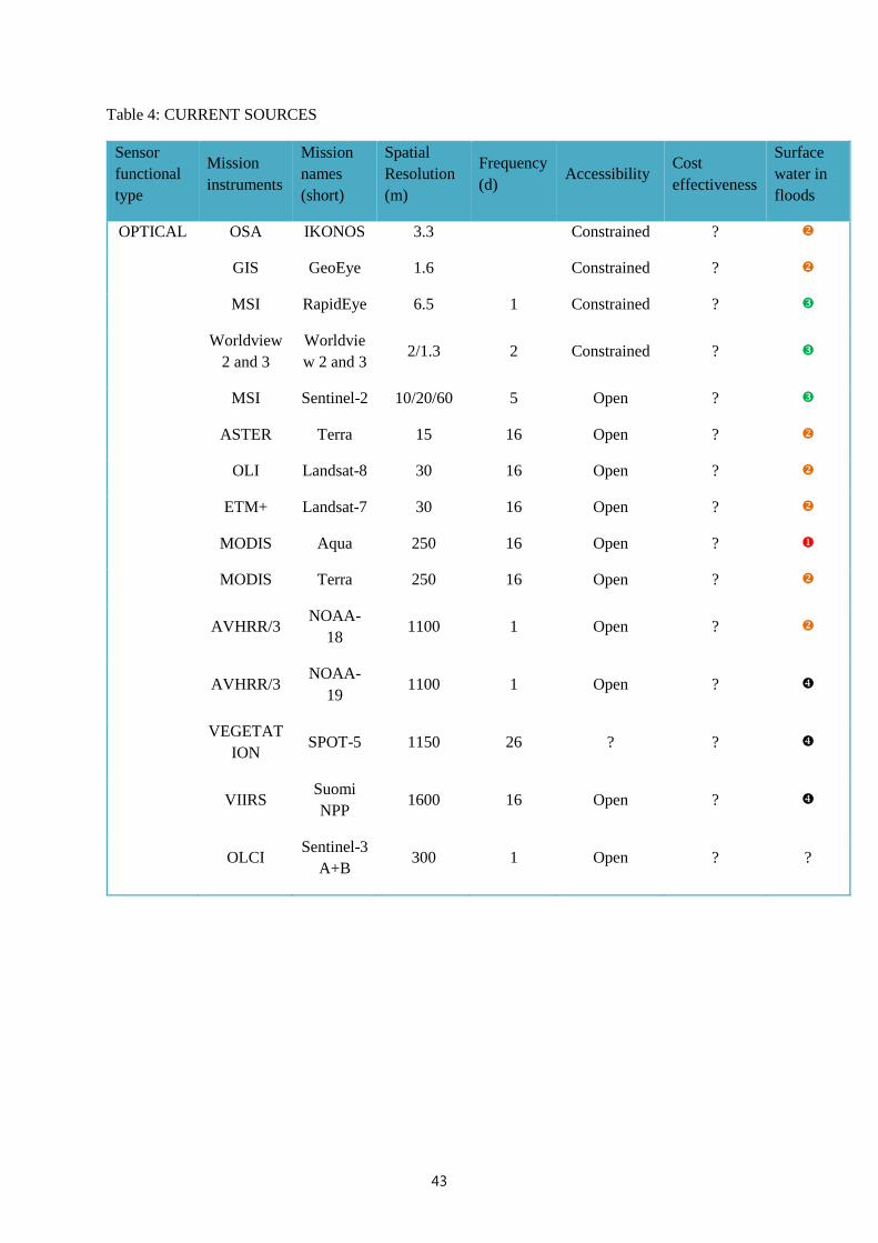
43
Table 4: CURRENT SOURCES
Sensor
functional
type
Mission
instruments
Mission
names
(short)
Spatial
Resolution
(m)
Frequency
(d) Accessibility
Cost
effectiveness
Surface
water in
floods
OPTICAL OSA IKONOS 3.3 Constrained ? ❖
GIS GeoEye 1.6 Constrained ? ❖
MSI RapidEye 6.5 1 Constrained ?
Worldview
2 and 3
Worldvie
w 2 and 3 2/1.3 2 Constrained ?
MSI Sentinel-2 10/20/60 5 Open ?
ASTER Terra 15 16 Open ? ❖
OLI Landsat-8 30 16 Open ? ❖
ETM+ Landsat-7 30 16 Open ? ❖
MODIS Aqua 250 16 Open ?
MODIS Terra 250 16 Open ? ❖
AVHRR/3 NOAA-
18 1100 1 Open ? ❖
AVHRR/3 NOAA-
19 1100 1 Open ?
VEGETAT
ION SPOT-5 1150 26 ? ?
VIIRS Suomi
NPP 1600 16 Open ?
OLCI Sentinel-3
A+B 300 1 Open ? ?

44
Which sensors to use to measure Vegetation and Land Cover metrics (NDVI, Albedo, fPAR and LAI)
Note: NDVI (Normalised Difference Vegetation Index)/ fPAR (fraction of PAR)/ PAR is photosynthetically Active radiation/Leaf Area Index (LAI).
Data
Currency
Sensor
Functional
Type
Mission
Instruments
Mission
Name
(Short)
Spatial
Resolution
(m)
Revisit
Period
(days)
Accessibility Launch
Date
End
Date NDVI Albedo fPAR LAI
Arc
hiv
al
Optical TM Landsat 5 30 16 Open Jul-82 Jun-13
MSS Landsat 1-
3
80 18 Open Jul-72 Sep-83 ❖ ❖ ❖ ❖
AVHRR/2 NOAA 7-
14
1100 1 Open Jun-81
❖
Curr
ent
Active
microwave
X-Band SAR TanDEM-
X
16 11 Open Jun-10
❖ ❖
X-Band SAR TerraSAR-
X
16 11 Open Jun-07
❖ ❖
S-Band SAR HJ-1C 20 31 Open Nov-12
❖ ❖
SAR
(RADARSAT
-2)
RADARS
AT-2
25 24 Constrained Dec-07
❖ ❖
Optical MSI RapidEye 6.5 1 Constrained Aug-08
❖ ❖ ❖ ❖

45
Data
Currency
Sensor
Functional
Type
Mission
Instruments
Mission
Name
(Short)
Spatial
Resolution
(m)
Revisit
Period
(days)
Accessibility Launch
Date
End
Date NDVI Albedo fPAR LAI
MSI Sentinel-2 10/20/60 5 Open Jun-15 ❖ ❖ ❖ ❖
ASTER Terra 15 16 Open Dec-99
OLI Landsat-8 30 16 Open Feb-13
❖
ETM+ Landsat 7 30 16 Open Apr-99
❖
Hyperion NMP EO-1 30 16 Open Nov-00 Oct-14
AWiFS RESOUR
CESAT-2
55 26 Open Apr-11
LISS-III
(Resourcesat)
RESOUR
CESAT-2
55 26 Open Apr-11
❖ ❖
MISR Terra 250 16 Open Dec-99
❖ ❖ ❖ ❖
MODIS Aqua 250 16 Open May-02
MODIS Terra 250 16 Open Dec-99
AVHRR/3 NOAA-18 1100 1 Open May-05
❖
AVHRR/3 NOAA-19 1100 1 Open Feb-09
❖
VEGETATI
ON
SPOT-5 1150 26 ? May-02 Dec-
14
❖ ❖

46
Data
Currency
Sensor
Functional
Type
Mission
Instruments
Mission
Name
(Short)
Spatial
Resolution
(m)
Revisit
Period
(days)
Accessibility Launch
Date
End
Date NDVI Albedo fPAR LAI
VIIRS Suomi
NPP
1600 16 Open Oct-11
Futu
re
Active
microwave
SAR (RCM) RADARS
AT C-1
50 12 Constrained 2018
❖ ❖
SAR (RCM) RADARS
AT C-2
50 12 Constrained 2018
❖ ❖
SAR (RCM) RADARS
AT C-3
50 12 Constrained 2018
❖ ❖
Optical LISS-III
(Resourcesat)
RESOUR
CESAT-
2A
5.8 26 Open 2015
❖ ❖
MSI
(Sentinel-2)
Sentinel-2
A
10 10 Open 2015
❖ ❖
MSI
(Sentinel-2)
Sentinel-2
B
10 10 Open 2016
❖ ❖
MSI
(Sentinel-2)
Sentinel-2
C
10 10 Open 2020
❖ ❖
LISS-IV RESOUR
CESAT-
2A
23.5 26 Open 2015
❖ ❖

47
Data
Currency
Sensor
Functional
Type
Mission
Instruments
Mission
Name
(Short)
Spatial
Resolution
(m)
Revisit
Period
(days)
Accessibility Launch
Date
End
Date NDVI Albedo fPAR LAI
HISUI ALOS-3 30 60 ? 2016
AWiFS RESOUR
CESAT-
2A
55 26 Open 2015
OLCI Sentinel-3
A
300 27 Open 2015/16
❖ ❖ ❖
OLCI Sentinel-3
B
300 27 Open 2017
❖ ❖ ❖
OLCI Sentinel-3
C
300 27 Open 2020
❖ ❖ ❖
VIIRS JPSS-1 1600 16 Open 2017
Source: Information derived from the Committee on Earth Observation Satellites (CEOS) Earth Observation Handbook (http://www.eohandbook.com/) and WMO Observing Systems Capability Analysis and Review
Tool (http://www.wmo-sat.info/oscar/).

48
2.15 Public and private sensors/satellites
There are three types of providers of satellite data; the national and multinational space agencies, most
of which are part of CEOS, commercial private industry providers and some private providers that are
linked to national space agencies such as ISRO for India and its affiliated company Antrix.
In tables 3 and 4 “open” and “constrained” satellite data sources are mentioned. Most open sources are
from the national and multinational space agencies and most constrained sources are the commercial
providers. The reason they are called constrained is because the End User License Agreement is usually
quite restrictive for sharing the raw data. Many of the commercial satellite data providers focus on very
high spatial resolution for defence, precision agriculture and precision mapping (e.g. cadastral)
purposes.
Most EO sources used to monitor ecosystem variables or renewable and non-renewable resources are
from the space agencies with an open data policy as that reduces or annuls the cost of data acquisition.
However, high value commodity monitoring does use the commercially available very high spatial
resolution data.
Although in the past much of the R&D was carried out by space agencies or large technological
institutes and academia, the last few years have seen an augmentation of applied research by
organisations such as GEO, NGOs, international development banks and the private sector. Thus, it is
crucial to adopt a pragmatic approach while entering the Big Data era, and work with all sectors. More
companies are getting involved in launching their own satellites or using satellite data products, and
some are taking the lead in some areas.
Even if governments used to rely only on their national satellites and sensors, they now understand the
urgent need to talk and work with private companies as they can offer satellite data services or products
which might be useful to manage Big Data and offer solutions. This section provides some examples
of private EO data sources; however this is by no means an exhaustive list.
There are an increasing number of companies that are investing in both satellites and the resulting data,
although there is also a wave of consolidation occurring with companies merging. At the same time
technology accelerators such as nanosats, cubesats, microsats etc. are evolving rapidly and augmenting
the space agencies and companies that have been launching and operating large systems with long
lifetimes. Thus, there is now a scale of operation of building and launching satellites of 100s to 1000
kilograms with long lifespans and very accurate measurements to smallsats or cubesats that weigh one
to a few kilograms but have limited lifespans.
This chapter provides information on available web based resources for the plethora of satellites
available and some guidelines on how to select the right satellite for the job at hand. The CEOS and
OSCAR databases focus more on the public sector systems.
Some of the private companies that provide highly relevant services are presented here but only as a
snapshot and without the intent of being complete. Some larger companies with a track record of
providing high spatial resolution and/or globally relevant data sets are:
• Digital Globe (https://www.digitalglobe.com/)
• AIRBUS Industries (http://www.satimagingcorp.com/satellite-sensors/other-satellite-sensors)
• Planet (https://www.planet.com/)
• Google Terra Bella (https://terrabella.google.com)

49
Many smaller dedicated companies exist that may have their own satellites such as the hybrid of space
agency and industry; the Chinese-Brazilian Earth Resources Satellite Program (CBERS) and the
collaboration between ISRO and ANTRIX in India. As a trend, increasingly space agencies are creating
joint venture type activities with private companies.
Open data policies are welcomed when it comes to public entities. Private satellite data providers are
generally not adopting the same policy because they can profit from selling such data. However, things
might change in that sector. In September 2015Will Marshall, CEO of Planet, announced the company
would open the access (under CC BY SA 4.0 open licence) to some high resolution satellite data
acquired by its constellation of microsatellites. Marshall made the announcement at the UN Assembly,
talking about how the data would contribute to the UN SDGs. In other words, their data can be used for
free, but whatever is produced using it must be made open in the same way (and this applies to value-
added products as well)13.
DigitalGlobe is a US leading global provider of commercial high‑resolution Earth imagery products
and services. It has activated FirstLook, the subscription service that provides emergency management
and humanitarian workers with fast, web-based access to pre and post event images of the impacted
area. DigitalGlobe provides images to help humanitarian crisis through Tomnod, another project that
uses crowdsourcing to identify objects and places in satellite images.
Therefore these companies acknowledge that while satellite imagery on its own is useful, greater benefit
comes from extracting meaningful information that can be used by first responder and recovery
agencies.
Another type of approach is by companies that have no space assets at all but harvest, harness and
display EO data from the actual providers such as Google Earth Engine, Amazon Web Services,
Facebook etc. Facebook's Internet.org project (population map) is an example that aims to beam
internet access to areas of the world that lack broadband access via drones and satellites. This internet
access can then be used access processed EO data providing geospatial information.
2.16 Future sensors and data architectures
The WMO OSCAR and CEOS EO sensors databases also include a comprehensive inventory of future
EO sensors.
In general EO sensors are becoming more sophisticated due to technological developments in the actual
sensors on the satellite platforms, the platforms themselves, the electronics, on board compression and
downlink rates to ground stations etc. These developments also lead to miniaturisation. Miniaturisation
leads to either enhanced capabilities in equal sized satellites (typically 500 to 1000 kg) or smaller
satellites right down to nano satellites or cubesats weighing only a few kilograms.
Another development in LEO sensors is the race between publicly funded and publicly available EO
data streams, and the commercial EO satellite sensors. In general, the coarser resolution sensors (pixel
size above 20 m) has been made available for free by most space agencies, and higher resolution data
has been provided at commercial rates. However, a gradual shift in publicly available spatial, temporal
and spectral resolution is going on: e.g. until the advent of Sentinel-2 in 2015 with freely available 10
m spatial resolution, Landsat with its 30 m pixels was the highest resolution free data. Thus commercial
operators now need to provide sub-10 m data to be competitive. The currently highest spatial resolution
13 http://www.eurisy.org/article-free-and-open-satellite-data-private-companies-join-in-the-game_18#sthash.0VQ20Ubf.dpuf

50
on offer from a commercial company is the WorldView-3 0.4 m panchromatic and the 1.3 m
multispectral and SWIR data.
Temporal resolution and area coverage are other areas of competition. Providing imagery on a ‘wall-
to-wall” basis, Landsat overpasses once every 16 days whereas Sentinel-2 (once both satellites 2A and
2B are launched) will provide imagery approximately once every 5 days world-wide. Spectral
resolution is also increasing, which will culminate in a shift from multispectral sensors (with typically
4 to 13 spectral bands) to imaging spectrometers (with 100s of spectral bands). Commercial operators
are providing increased temporal resolution by either having their EO sensors be pointable in all
directions in space, or by launching “swarms” of sensors such as the RapidEye constellation and
increasingly cubesat and nanosat constellations such as the SkySat constellation of 7 high resolution
satellites complementary to Planet’s existing medium resolution 60-satellite fleet. The former
enable regular, rapidly updated snapshots of select areas of the globe at sub-meter resolution; the
latter regular, global coverage at 3-5 meter resolution.
Geostationary sensors, which were exclusively the domain of meteorological coarse scale
measurements, are now providing higher spatial resolution imagery with more spectral bands,
especially adding bands in the blue and green wavelengths, making them much more useful for non-
meteorological use. The thermal bands are also becoming finer in resolution. The most recent type of
advanced GEO sensor is the Himawari-8, satellite from Japan which is positioned over Indonesia at
36000 km. It views half of the globe every 10 minutes, with spatial resolution of 500 to 2000 m pixels.
Several more Himawari type sensors (known as the GOES-R series, with a first launch for the Americas
accomplished late 2016) will be placed in geostationary orbits to cover the Americas and Africa and
Europe. There is fast progress in developing non-meteorological use of this advanced type of
geostationary EO data.
The potential new data architectures are also critical for the future of EO and the benefits of the use of
data. EO programmes of space agencies are facing a number of trends which are driving the need for
change in the ways in which data are processed, analysed and distributed. As the change is becoming
crucial, the CEOS Chair (CSIRO) for 2016 has proposed to study the issues around next-generation EO
data system architectures (CEOS Future Data Architectures (FDA) ad-hoc team), and the opportunities
offered by approaches such as the Data Cube (see2.17) and commercial cloud storage and processing
solutions. The ad-hoc team looked at the relevant current initiatives undertaken by CEOS; lessons
learned from early prototypes, identified the key challenges and expressed some recommendations. An
interim report is now available on CEOS website14. A more comprehensive report will be delivered in
2017.
Maximising the value of EO is actually a fundamental driver for space agencies. In recent years there
has been a steady trend across space agencies toward a greater integration of diverse EO data for various
applications in land, water, climate issues. The increased integration produced a more diverse range of
applications, which leads to complexity in the value chain when observations are combined with
analytics to meet multiple user requirements.
Another key message for NSOs is that, in addition to free and open data, space agencies realise how
desirable it becomes now to get free and open access to analysis software and tools that facilitate the
14 CEOS Future Data Access and Analysis Architectures Study - Interim Report (October 2016): http://ceos.org/meetings/30th-ceos-
plenary/ and more precisely here: http://ceos.org/document_management/Meetings/Plenary/30/Documents/5.2_Future-Data-Architectures-
Interim-Report_v.1.pdf

51
use of EO data. The CEOS Data Cube initiative, based on the Australian Geoscience Data Cube
(AGDC), see section 2.17) is an example of that trend. The project relies on open source software for
the creation of data cubes (ingesting satellite data) and the interaction with data cubes (application
programming interfaces= APIs). Open source software would undoubtedly stimulate application
innovation and the increased use of satellite data since these advanced technologies can be utilised
globally and even by developing countries that are not traditional users of satellite data,
This FDA report stressed that CEOS agencies will need to continue working on that issue given its
stakes. “Future work should help users benefit from all relevant CEOS data at all stages –
complementing past efforts which have emphasised unity of ‘discovery’, without fully addressing the
significant challenges in the analysis and exploitation of disparate or incompatible data after discovery.”
Figure 14: Future Global Data Flow Options for National Forest Monitoring Systems
2.17 Example: Data Cube initiatives
Australian Geoscience Data Cube
The Australian Geoscience Data Cube (AGDC) is a new collaborative approach for storing,
organising and analysing the vast quantities of satellite imagery and other Earth Observations, making
it quicker and easier to provide information on issues that can affect all Australians. The AGDC is
developed and maintained by a partnership between Geoscience Australia, the Commonwealth
Scientific and Industrial Research Organisation (CSIRO), and National Computational Infrastructure
(NCI).
The AGDC makes standardised and calibrated satellite data available in structures on a range of
processing platforms which can be either local, remote or cloud based. The AGDC software is also
optimised for use by High Performance Computing facilities, such as the ‘Raijin’ facility at the National
Computational Infrastructure in Australia. The AGDC is composed of a series of data structures and

52
tools which facilitate the efficient analysis of very large standardised and calibrated gridded data
collections, like satellite data, for multiple purposes (Figure 15). This enables a user to easily apply the
full potential of satellite data to real-world challenges like agricultural productivity and monitoring of
industrial impact on the landscape.
Figure 15: The Data Cube provides a common analytical framework to allow multiple data sources
(on the left) to produce information for multiple uses (on the right)
Standardisation and calibration increases the value which can be derived from EO, and other sources of
large gridded datasets. It allows for the rapid development of information products to enable informed
decision making across government and industry.
This standardisation and calibration is important for another reason. It means that products created by
different users to address different problems can be integrated. This ability to integrate information will
be critical to solving big national challenges. For example, efforts to improve agricultural productivity
are more effective if soil moisture information can be integrated with information on crop health and
on forecast precipitation.
Proving the concept
The AGDC has been used to complete analyses that were previously impractical. For example, a
recently completed study mapped observations of surface water across all of Australia for the period
1998 to 2012 at a nominal 25 metre resolution. This analysis would have taken 4-8 years under a
traditional model, but can now be produced in less than 4 hours using the AGDC. This product is now
an information source for the National Flood Risk Information Portal (Figure 16) helping communities
understand, and plan for, potential future flooding.
The section of land in Figure 15 shows the channel country adjacent to the Simpson Desert with
infrequently observed water in red through to permanent water bodies in blue.

53
Figure 16: Water Observations from Space (WOfS) mapped surface water observations for all of
Australia at 25 metre resolution using data from 1998 to 2012.
Key characteristics
The use of standardised and calibrated data is a key characteristic of the AGDC. In the past the
calibration of EO data has been performed on a per-application basis for subsets of data. This can be
inefficient and results in large overheads. By calibrating all data to the same standard it becomes
immediately usable by many different user groups, eliminating up to 80% of the non-productive ‘start
up’ activity often required in a traditional approach.
Another key characteristic of the data cube is it maintains every unique observation and makes it
available for analysis. This contrasts with traditional approaches where technical limitations mean only
small subsets are used. This enables the full ‘time series’, all of the observations acquired by the
satellites over many years, to be put to work. This is critical because many important phenomena only
become apparent when monitored regularly over time.
The final key characteristic of the AGDC is its ability to deliver ‘economies of scale’. The same costly
supercomputing facilities and data stores, the infrastructure that enables these levels of performance to
be achieved, can be used for multiple purposes. The ability to realise these economies of scale is of
increasing importance.
Data volumes that are already impossible to manage on a per-agency basis are scheduled to grow
exponentially as new satellites from the USA, Europe, Japan and elsewhere give us access to more data
than ever before. An approach which enables investment in shared infrastructure will be critical if we
are to benefit from this data.
The unique way in which the AGDC organises data enables it to be rapidly manipulated in a single high
performance computing environment (Figure 17) for many different purposes. The AGDC organises
images from multiple sources and times, such as the images on the left, into stacks of tiles (on the right).
The top of the stack is the most recent observations. As a result, the AGDC can help us embrace the
‘data deluge’.

54
Figure 17: AGDC organisation process
More information can be found at www.datacube.org.au and the source code is available on GitHub at
https://github.com/data-cube/agdc-v2.
Role of CEOS and the Data Cube technology
Many countries lack the knowledge, infrastructure, and resources to access and use space-based data.
Countries have expressed a desire for support from CEOS by providing search & discovery tools, cloud-
based storage and processing, and training & capacity building.
CEOS is leading several projects to demonstrate data services tools and build an architecture that
supports a growing volume of data. Some countries (Kenya and Colombia) have already asked CEOS
to help them building such an environment to manage Big Data on EO, and making them active pilot
projects for the Data Cube. The objective is these pilot projects will provide a solid foundation for future
operational systems to be funded and managed by UN organisations and individual countries.
While providing architecture and tools for countries to access and utilise satellite data, and also the
training and capacity building necessary to use those tools and manage satellite data, CEOS is
developing prototype projects to demonstrate those tools and services. CEOS is evaluating advanced
technologies in its architecture and tools, such as Data Services Platforms and Data Cubes based on
cloud computing.
Countries and regions with on-going and future Data Cube projects:
• Australia
• Kenya
• Colombia
• Switzerland
• South East Asia
NSOs interested in these future data programs are strongly encouraged to get in touch with the CEOS
Systems Engineering Office as they are building a global system to organise the implementation of Data
Cubes in countries.

55
2.18 Recommendations on selecting appropriate EO sources
As EO transforms from relying on a few publicly available well defined EO sensors, such as MODIS
and Landsat sources, to a much larger array of sensors with significantly enhanced specifications, the
trend will be towards more data, with greater accuracy and precision being a part of the new Era of Big
Data.
Before using EO satellite data, NSOs need to consider some key questions (cf. decision tree in Figure
33, Chapter 5) to decide whether or not using EO will assist in achieving their objectives and outputs
effectively. The research question can guide the user to decide what EO data sources might be
appropriate and useful.
If EO data is chosen as a data source, consider the best sensors to use (cf. CEOS or OSCAR of WMO
databases), depending on various previously defined criteria. The global initiative GFOI is a good
example of land surface monitoring, as a core data stream that has been well defined and is currently
operational.
Even though the accuracy is generally lower for one pixel than with a field data measurement for the
same field plot, EO products should still be considered an important alternative data source, as EO
imagery can provide information with greater spatial extent, spatial density, and/or temporal frequency
than any field-based (point-based) observation networks. The cost per unit area sampled and per
variable will significantly reduce, as EO satellite data become more prevalent.
By using smart methods for retrieving more and more valid information from EO data, the emphasis
can shift increasingly from field data to EO data. NSOs can benefit from using more EO data, where
relevant and appropriate, to replace or complement their results and analysis.
Another point to highlight is the importance of the public data provided by all national space agencies.
More and more private companies invest in satellites and launch their own missions to respond to
immediate, punctual and operational requests from their users. Despite the great interest in these new
activities in space, it is important to stress here the global coverage and continuity in time (missions
planned for the next decades); two main characteristics that were only provided by public and national
space agencies until now.
This fundamental aspect certainly needs to be taken into account for NSOs if they wish to use EO
satellite data in certain situations. For example, if the area of interest is how a relevant process, such as
erosion, land degradation, crop types, forest cover, wetlands extent, evapotranspiration, urban
expansion has developed over the last 30 years it is evident that the Landsat time series is the only
source of data. However, for example if the issue of interest is recent coal seam gas extraction has
caused any subsidence, then public or private high resolution SAR images in interferometric mode
would be most appropriate. These sources would give accuracies of millimetres deformation at any
temporal scale captured since the launch of the satellites. If an environmental or natural resources
baseline geospatial map is required, it could be best to opt for the highest spatial resolution imagery
accessible.
With the concept of ARD global coverage and continuity are important issues that involve a significant
amount of resources to create an ARD type EO Data Cube. This is only worthwhile if there will be
multiple uses made of the data for the past, present and future.

56
2.19 Illustrations
The United Nations has identified 17 Sustainable Development Goals (SDGs) to address challenges of
economic and social development and environmental sustainability. For each of the SDGs, the UN has
identified multiple targets and is developing indicators countries will use to track and report progress.
To achieve the SDGs, geospatial information and Earth observations, collected at local, national and
global levels, and supported by the best science, tools and technologies, can serve critical, insightful
roles in monitoring targets, tracking progress, and helping nations make mid-course corrections.
Combined with demographic and statistical data, these sources help enable nations to analyse and model
conditions, create maps, and monitor change over time in a consistent and standardised manner
(http://www.earthobservations.org/).
Below 2 SDGs are illustrated, which have an identified earth observation measurable component.
Examples of utilisation of EO satellite data for the UN SDGs (2030 Agenda)

57

58

59
SDGs and EO data: satellite data used in a varied range of applications (GEO document) 15
15 GEO “Supporting Official Statistics in Monitoring the SDGs”, March 2016 – 47th UN Statistical Commission in NYC. More here:
http://www.earthobservations.org/documents/meetings/201603_eo_sdgs_ny/2016_geo_un_flyer.pdf and here as well:
http://www.earthobservations.org/geo_sdgs.php

60
Source: CEOS/GEO EO4EDGs Initiative, 2017
1.4 1.5 1.4.2
2.3 2.4 2.c 2.4.1
3.3 3.4 3.9 3.d 3.9.1
5.a 5.a.1
6.1 6.3 6.4 6.5 6.6 6.a 6.b 6.3.1 6.3.2 6.4.2 6.5.1 6.6.1
7.2 7.3 7.a 7.b 7.1.1
8.4
9.1 9.4 9.5 9.a 9.1.1 9.4.1
10.6 10.7 10.a
11.1 11.3 11.4 11.5 11.6 11.7 11.b 11.c 11.1.1 11.2.1 11.3.1 11.6.2 11.7.1
12.2 12.4 12.8 12.a 12.b 12.a.1
13.1 13.2 13.3 13.b 13.1.1
14.1 14.2 14.3 14.4 14.6 14.7 14.a 14.3.1 14.4.1 14.5.1
15.1 15.2 15.3 15.4 15.5 15.7 15.8 15.9 15.1.1 15.2.1 15.3.1 15.4.1 15.4.2
16.8
17.2 17.3 17.6 17.7 17.8 17.9 17.16 17.17 17.18 17.6.1 17.18.1
Sustainable Development Goals
Earth Observations in Service of the Agenda 2030
Direct measure or indirect support
Indicator
Goal
Contribute to progress on the Target yet not the Indicator per se
Target

61
3. Methodology
3.1 Introduction
This chapter presents an overview of methodology for using spectral bands or frequencies generated
from earth observation (EO) data to estimate quantities of interest to NSOs. The chapter follows on
from Chapter 2, which describes the sources of EO data, and addresses the question, ‘now that we have
the data, how do we use it?’.
EO images, and the data that are extracted from them, fall into the category of ‘big data’. This term is
generally used to describe large datasets that are challenging to store, manage and analyse. For many
NSOs, traditional data management and analysis tools are inadequate. Other issues include choice of
appropriate statistics, consideration of the quality and accuracy of the data and results, and validation
and interpretation of the outputs.
The development of techniques and tools for the analysis of EO data has been occurring for over a
decade. However, the increasing resolution and availability of EO data has meant that it is now feasible
for organisations and agencies such as NSOs to consider including this data source in their systems.
This chapter commences in Section 3.2 with a discussion of the types of estimates relevant to NSOs
that can be derived from EO data. These include official statistics for use at a national level, as well as
statistics related to the 2030 Agenda for Sustainable Development. An overall description of the
approach to analysing EO data is provided in Section 3.3. Three broad steps involved in this approach
include pre-processing the images and data, analysing the data to obtain the required estimates, and
validating the results. These steps are described in more detail in Sections 3.4 to 3.7. The chapter closes
with a summary in Section 3.8.
3.2 EO data and official statistics
Sustainable Development Goals
The use of EO data for official statistics conforms to the 2030 Agenda for Sustainable Development,
through the use of a wider range of data to support implementation of the Sustainable Development
goals, targets and indicators (http://unstats.un.org/sdgs/indicators/indicators-list/). As described in
Section 2.19, EO data can contribute to many of the SDG targets and indicators. Examples of SDG
targets and indicators that are directly relevant to EO data include the following:
• 2.4 By 2030, ensure sustainable food production systems and implement resilient agricultural
practices that increase productivity and production, that help maintain ecosystems, that
strengthen capacity for adaptation to climate change, extreme weather, drought, flooding and
other disasters and that progressively improve land and soil quality.
o 2.4.1 Proportion of agricultural area under productive and sustainable agriculture.
• 6.3. By 2030, improve water quality by reducing pollution, eliminating dumping and
minimising release of hazardous chemicals and materials, halving the proportion of untreated
wastewater and increasing recycling and safe resuse globally.
o 6.3.2 Percentage of bodies of water with good ambient water quality.
• 6.6 By 2020, protect and restore water-related ecosystems, including mountains, forests,
wetlands, rivers, aquifers and lakes.
o 6.6.1 Change in the extent of water-related ecosystems over time.

62
• 15.1 By 2020, ensure the conservation, restoration and sustainable use of terrestrial and inland
freshwater ecosystems and their services, in particular forests, wetlands, mountains and
drylands, in line with obligations under international agreements.
o 15.1.1 Forest area as a proportion of total land area.
o 15.1.2 Proportion of important sites for terrestrial and freshwater biodiversity that are
covered by protected areas, by ecosystem type.
• 15.2. By 2020, promote the implementation of sustainable management of all types of forests,
halt deforestation, restore degraded forests and substantially increase afforestation and
reforestation globally.
o 15.2.1 Forest cover under sustainable forest management.
o 15.2.2. Net permananet forest loss.
• 15.3 By 2030, combat desertification, restore degraded land and soil, including land affected
by desertification, drought and floods, and strive to achieve a land degradation-neutral world.
o 15.3.1 Proportion of land that is degraded over total land area
Anderson et al. (2017) provide a number of examples that illustrate the use of EO in the service of the
2030 Sustainable Development Goals. The following advantages are highlighted: enablement of
informed decision-making and monitoring of the expected results; improvement of national statistics
for greater accuracy; assurance that the data are “spatially-explicit”; fostering of synergy between the
SDGs and multilateral environmental agreements by addressing cross-cutting themes such as climate
and energy; and facilitation of countries’ approaches for working across different development sectors.
3.2.1 Environmental and agricultural statistics
A current major focus of EO data analysis is on deriving environmental and agricultural statistics. Three
specific examples of statistics that can be derived from EO data are land cover, land use and land cover
change. These are defined in the FAO Global Strategy16 report as follows: land cover is the observed
(bio) physical cover on the Earth’s surface; land use is the use made of land by humans; and land change
studies attempt to describe where and what change is occurring over time, at what rate and perhaps
why.
Other agricultural statistics include crop identification and crop yield. Crop identification and crop yield
case studies are detailed in Chapter 4. For further information about using EO data for crop
identification and crop yield, refer to the FAO Handbook on Remote Sensing for Agriculture Statistics.
These statistics can be tabulated or displayed graphically, as illustrated in Figure 18 for Chiapas,
Mexico.
16 Global Strategy 2017. Handbook on Remote Sensing for Agricultural Statistics. Rome, www.gsars.org, 250pp.

63
Figure 18: Examples of geographic display of statistics relevant to the SDG indicators that can be
obtained in full or in part by EO data. Use of INEGI’s Land Use and Vegetation Map Series in the
Digital Map of Mexico (various scales available). Left: Indicator 15.2.1 Progress towards sustainable
forest management. Right: Indicator 15.2.2 Net permanent forest loss, estimated changes in tropical
broadleaf evergreen forest in Chiapas based on satellite images from 2006 to 2013.
Source: Figures extracted from Integrating Statistical and Geospatial Information: Experience in Mexico. Presentation by Mr. Rolando
Ocampo, Vice President, INEGI, Mexico. Meeting organised by UNSD on Geospatial Information and Earth Observations: Supporting
Official Statistics in Monitoring the SDGS, New York, 7th March 2016.
Another example of graphically displaying environmental and agricultural statistics derived from
satellite imagery is the Global Forest Change map by Hansen, Potapov, Moore, Hancher et al (2013).
Forest loss, forest cover loss and gain and percentage of tree cover are identified from time series
analysis of Landsat images and depicted on an interactive global map in Google Earth Engine. A section
of the map is below in Figure 19.
Figure 19: Global Forest Change map view of South America

64
See https://earthengineparnterns.appspot.com/science-2013-global-forest for more information and to
view the map.
3.2.2 Other statistics
Many other statistics of interest to NSOs can be obtained from EO data. Examples that address the
SDGs include water quality detection (Dekker et al., 2016), urban change (Taubenboch et al.,2012;
Esch et al., 2012) and natural disaster risk assessment (Geib and Taubenboch, 2013). Anderson et al.
(2017) also describe examples of global crop monitoring (by GeoGLAM), electricity access (visualised
using night time satellite imagery to assess the location and spread of electric lighting) for SDG 7.1, air
quality (by monitoring aerosols, hot spots and forest fires , SDG11.6) and biodiversity (by EO
monitoring of protected areas and potential criminal activity, SDGs 14 and 15).
Different forms of EO data can be combined to provide relevant statistics. For example, drones are now
being used extensively as EO data sources in their own right and in combination with satellite and radar
data. They are also being used in combination with traditional data sources such as surveys, and with
other big data sources such as mobile phone and social media data. For example, Steele et al. (2017)
give an example of combining EO and mobile phone data to obtain poverty estimates.
It is important to note that different definitions of quantities of interest can affect the calculation of the
estimates. This is described in the FAO Global Strategy report for the case of land cover change:
substantial differences were found in 11 cover classes derived from four different global databases. The
report notes (p. 23) that “this does not mean that the figures are inaccurate (as they relate to different
definitions of class membership); rather, they are inconsistent, especially where few classes are used.”
For this reason, a common Land Cover Classification System (LCCS)17 has been developed by the FAO
and UNEP, as detailed in the report18. The SEEA Central Framework19 is a useful international standard
for environmental accounting and its land cover classification is based on the set of rules and classifiers
set out in the LCCS.
3.3 General approach to analysing EO data
3.3.1 Steps in the analysis of EO data
The analysis of EO data can be divided into three broad steps, as follows:
The Pre-processing step is critical to successful analysis of big data, and the quality and integrity of
the obtained estimates. This step involves the following considerations:
17 Also refer to the LCCS2 http://www.fao.org/docrep/008/y7220e/y7220e00.htm and LCCS3 http://www.fao.org/3/a-i5232e.pdf)
18 Report reference: (http://gsars.org/wp-content/uploads/2016/08/TR_Information-on-Land-in-the-Context-of-Ag-Statistics-180816.pdf,
Information on Land in the Context of Agricultural Statistics, Technical Report Series GO-15-2016). 19 SEEA Central Framework https://unstats.un.org/unsd/envaccounting/seearev/seea_cf_final_en.pdf
Pre-processing Analysis Evaluation

65
• Data storage: This includes storage of the EO images and/or extracted data, and of the statistics
and derived products obtained from the analysis of the data.
• Data management: This includes management of the EO images and extracted data.
• Data quality: This includes critical evaluation of the data extracted from the EO images with
respect to its overall capacity for analysis and ability to provide reliable, accurate statistics.
• Other information sources: This includes identification, collation, storage, management and
evaluation of other supporting data that can be used in the analysis step.
• Software: Based on the above considerations, this includes identification of appropriate,
available software products that can be employed to help with the pre-processing step.
The Analysis step involves the following considerations:
• Overall aim: This includes defining the overall aim, such as provision of particular national
statistics or a SDG indicator; and defining the corresponding statistical estimates, predictions
or inferences that are to be obtained from the analysis.
• Data: This includes determining which subset of the stored data will be used in the analysis,
and whether the analysis will be based solely on the EO data or in combination with other data
sources.
• Analytic method: This includes selection of a general approach and specific technique for
extracting the required quantities, based on the aim and available data.
The Evaluation step involves the following considerations:
• Critical assessment of the results: This step involves collating, assessing and interpreting the
results of the analysis.
• Accuracy assessment: This includes a comparison between observed values and predicted
estimates where possible, assessment of the uncertainty or precision of the results, and
evaluation of the replicability of the results.
• Other concerns: This includes consideration of any other potential biases or concerns with the
results and their interpretation.
These steps are described in detail in Sections 3.4 to 3.7.
3.3.2 Implementation of methodology
Various NSOs have devised plans for implementing the analysis of EO data. These plans incorporate
the above steps in different ways.
As illustration, Figure 20 shows the template proposed by Denmark to facilitate the pathway from EO
data collection to estimation of relevant statistics and integration into NSO operations.
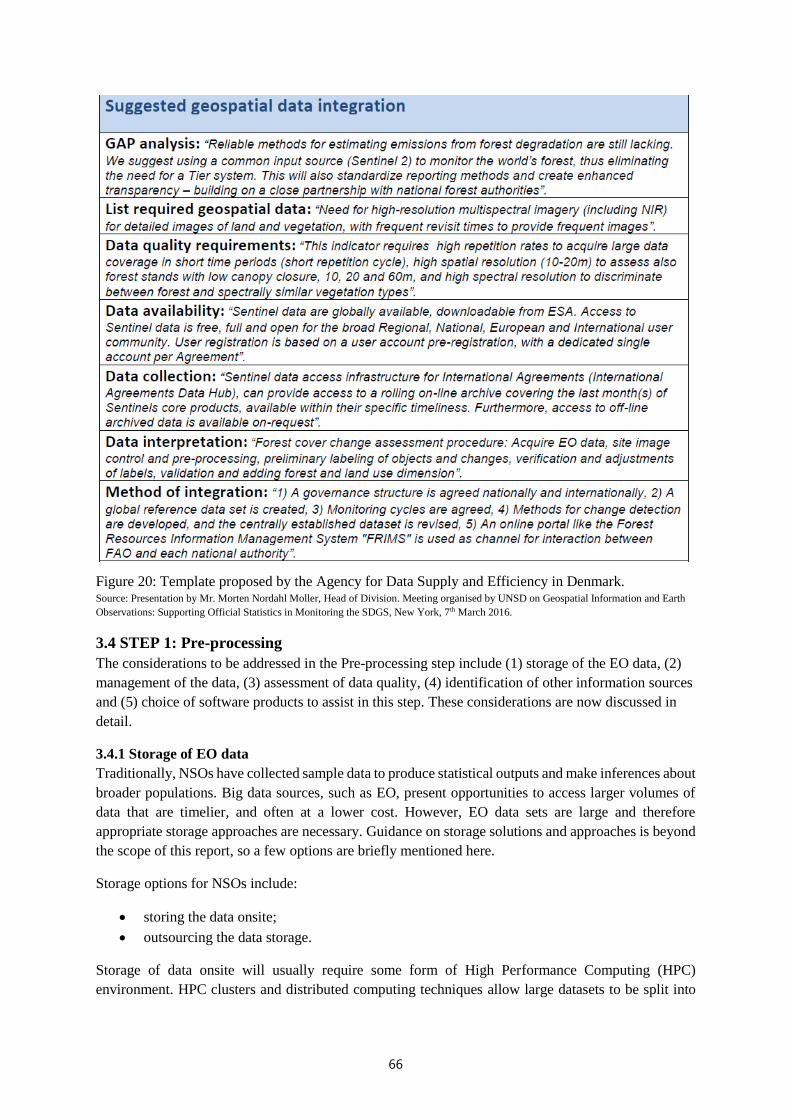
66
Figure 20: Template proposed by the Agency for Data Supply and Efficiency in Denmark. Source: Presentation by Mr. Morten Nordahl Moller, Head of Division. Meeting organised by UNSD on Geospatial Information and Earth
Observations: Supporting Official Statistics in Monitoring the SDGS, New York, 7th March 2016.
3.4 STEP 1: Pre-processing
The considerations to be addressed in the Pre-processing step include (1) storage of the EO data, (2)
management of the data, (3) assessment of data quality, (4) identification of other information sources
and (5) choice of software products to assist in this step. These considerations are now discussed in
detail.
3.4.1 Storage of EO data
Traditionally, NSOs have collected sample data to produce statistical outputs and make inferences about
broader populations. Big data sources, such as EO, present opportunities to access larger volumes of
data that are timelier, and often at a lower cost. However, EO data sets are large and therefore
appropriate storage approaches are necessary. Guidance on storage solutions and approaches is beyond
the scope of this report, so a few options are briefly mentioned here.
Storage options for NSOs include:
• storing the data onsite;
• outsourcing the data storage.
Storage of data onsite will usually require some form of High Performance Computing (HPC)
environment. HPC clusters and distributed computing techniques allow large datasets to be split into

67
blocks and run simultaneously on multiple nodes for faster computational time. Results from each node
are then combined in statistically sensible ways.
Setting up a HPC system that is capable of dealing with current – and future – EO data can be expensive
in terms of infrastructure, training, upkeep and currency. For these reasons, outsourcing data storage is
an appealing alternative. For example, there are various cloud-based storage solutions such as those
offered by Microsoft and Amazon Web Services, or local trusted companies can be considered.
Another option is to use third party or open data. Open EO data are becoming increasingly prevalent
and are now part of the remit of many EO data sources (e.g., Copernicus). Using analysis-ready data
can further simplify the process by eliminating not only problems of storage but also most of the pre-
processing burden. Data Cubes described in Chapter 2, for example, have HPC capability, and make
standardised and calibrated satellite data available in structures available on a range of processing
platforms which can be either local, remote or cloud based. Online and free data catalogues combined
with on-line modelling platforms such as the GEE – Code Editor may also be applicable.
3.4.2 Management of EO data
Management of EO data typically involves processing images to analysis ready data (ARD).
As described in Chapter 2 and in the previous section, some countries have a Data Cube or other sources
of ARD available. This can usually be analysed without further pre-processing. However, it is important
that other considerations, such as assessment of bias and validation of results, are still undertaken. These
issues are described in more detail in subsequent sections of this chapter.
For many NSOs, ARD data may not yet be available. As discussed in Chapter 2, raw EO data are not
able to be used for analysis unprocessed because this would lead to inaccurate results based on varying
sun-angles and sensor geometries, noise, haze and distortion of the underlying imagery data. Different
pre-processing levels are conducted in order to increase the quality of the imagery data.
The goal of the pre-processing is to extract the pure spectral information reflected from the surface of
the earth and recorded by the sensor without any obscuring aspects. This is done through so-called
correction algorithms, namely, geometric correction and radiometric correction. These algorithms filter
out and correct for specific and defined noise parameters. The goal of the geometric correction is to
improve the accuracy of surface spectral reflectance, emittance, or back-scattered measurements ob-
tained using a remote sensing system. This pre-processing step is also known as detector error
correction, or atmospheric and topographic correction. The radiometric correction deals with
atmospheric particles which can obscure spectral information.
In addition to these Top of Atmosphere satellite imagery corrections, “masking” of data is also required.
Masking refers to the process of detecting and then “masking” out obscuring artefacts such as cloud
cover, cloud shadow, fire clouds, water, and so on. All these corrections are an integral part of creating
Analysis Ready Data (ARD).
With some investment of time and skills, NSOs can set up a system to process raw satellite imagery
data to the ARD stage using either proprietary or open-source software.
Open-source software is potentially less expensive to set up and has the advantage of providing
independence from proprietary systems. This has advantages of allowing the software to be customised
and linked to a broader range of software products and systems that are already embedded in the

68
organisation. Moreover, there is often a large open source community that can provide support and
solutions to problems. On the other hand, proprietary software can be seen to be more reliable from the
client or consumer’s perspective, and may have the advantage of greater technical support. (Trevithick
and Gillingham, 2009). Software products are discussed further in Section 3.4.5.
A detailed system that uses open-source software to process raw satellite imagery data to ARD is
described in Section 3.4.6. This system was developed by the Remote Sensing group in the Queensland
Department of Science, Information Technology and Innovation (DSITI) in Australia. The system was
developed prior to the creation of the Australian Data Cube and has been actively used for more than a
decade. It uses Landsat data available from the United States Geological Survey (USGS) website and
applies a number of open source software packages that translate data formats, make atmospheric
corrections and program the image-processing. An example of how this processed data is used to
identify cropping activity and land use is outlined as a case study in Chapter 4.
3.4.3 Quality assessment of EO data
Traditionally, NSOs have collected sample data to produce statistical outputs and make inferences about
broader populations. Big data sources, such as EO, present opportunities to access larger volumes of
data that are timelier, and often at a lower cost.
There is a misconception that big data sources, such as EO, will be statistically valid simply due to the
magnitude of data available. Although increasing sample size can reduce sampling errors, it does not
reduce other sources of statistical bias such as measurement error. Further, data sets derived from these
sources are not necessarily random samples of the target population NSOs want to make inferences
about, therefore increasing the size of the dataset may not reduce sampling error or improve the quality
of the estimates.
In addition, big data sources have their own specific issues which can impact on statistical validity.
These include accumulation of errors (noise) and potential spurious correlations, as well as algorithmic
instability that can lead to inaccurate estimates. The different sources of data, and their aggregation, can
also lead to statistical biases (Fan, Han and Liu, 2014).
Some of these challenges of using big data for statistical purposes can be addressed by using appropriate
methodologies, depending on the data source and intended outputs. Examples of different
methodological techniques for EO data specifically are described in this chapter. However, it should be
noted that these methodologies will not counter issues related to data quality, data representativeness
or other related issues. This is discussed further in Section 3.7.3.
3.4.4 Other information sources
EO data can be analysed on its own, or with other datasets. The choice of other datasets depends on
the following considerations:
• Aim: Different datasets will be required for different purposes, based on the required
estimates, selected method for analysis, spatial and temporal resolution and scope of the
analysis, quality of the available EO data, and so on.
• Access: Datasets can include existing resources held by the NSO and/or they can be obtained
from external parties. Access considerations also include intellectual property, confidentiality,
cost, reputation, and continuity of access.

69
• Content: A wide range of data can potentially complement EO data in an analysis, such as
censuses, household or agricultural surveys, administrative data, environmental and
meteorological data.
The FAO report on a Global Strategy for Improving Agricultural and Rural Statistics (2016) provides
advice about constructing and maintaining a Minimum Set of Core Data (MSCD) that includes EO and
other spatial and non-spatial information in a Master Sample Frame (MSF) database. The MSF is
constructed by combining satellite images classified by geo-referenced land use and digitised
administrative data, digitised enumeration areas, and overlaying this with population and agricultural
census data, other relevant data such as a register of commercial farms, and an area frame.
(http://gsars.org/wp-content/uploads/2016/08/TR_Information-on-Land-in-the-Context-of-Ag-
Statistics-180816.pdf, Information on Land in the Context of Agricultural Statistics, Technical Report
Series GO-15-2016)
Many NSOs are in various stages of implementing systems to integrate EO data with other data for
official statistics and SDGs. For example, Table 5 shows how Mexico envisages the use of different
resolutions of satellite imagery for national statistics and to support the related SDGs. These statistics
can be geographically displayed as illustrated in Figure 18.
Table 5 Integrating Statistical and Geospatial Information: Experience in Mexico.
Source: Presentation by Mr. Rolando Ocampo, Vice President, INEGI, Mexico. Meeting organised by UNSD on Geospatial Information and
Earth Observations: Supporting Official Statistics in Monitoring the SDGS, New York, 7th March 2016.

70
3.4.5 Software products
There is a range of proprietary and open source software products available for working with EO data.
The products can be used to assist with preparation, storage and management of data. This chapter does
not make recommendations on software product because the most appropriate tool will vary for
individual NSOs.
When choosing a product, NSOs should consider the capabilities and experience of their staff using
different software, cost if choosing a commercial product, and long term accessibility if choosing an
open source product. For example, if the NSO built a statistical collection around data produced using
an open source product, how would they be impacted if the provider started charging for access and
have contingency plans in place.
The list of software available is increasing rapidly. Some popular products that are available now are
briefly described here.
Hadoop is a popular technology related to big data management (Scannapieco, Virgillito and Zardetto
(2013). It is an open-source software project, developed by the Apache Software Foundation,
targeted at supporting the execution of data-oriented application on clusters of generic hardware.
The main components of Hadoop are HDFS, which sends tasks to multiple cores for processing,
and MapReduce, which keeps track of the data packets and combines the results of the processes.
Many products are now available that use Hadoop as a platform and provide improved interfaces
for easier engagement by end-users. Popular current examples include Spark and its derivatives
(such as Sparkling Water and Steam), and Tensor Flow.
GDAL/OGR - Geospatial Data Abstraction Library (reading and writing raster and vector geospatial
data formats) - most of the commonly used geospatial software applications use GDAL/OGR.
GDAL supports more than 140 raster formats; OGR supports over 80 vector formats (see Warmerdam
et al. (2016) for more information).
Some software packages (e.g. raster in R (R Core Team, 2016)) allow manipulation of data too large to
load into memory in its entirety by only creating structure information about the data, and processing
in chunks when manipulating the data itself.
GIS - System for Automated Geoscientific Analyses (SAGA) SAGA is open source software which
is intended to give scientists an effective but easily learnable platform for implementing geoscientific
methods and enables the user to perform vector and raster based spatial analysis, edit and manipulate
diverse data and store it in a format which allows sharing with other GIS communities and commercial
software packages. Further, it can perform interpolations using triangulation, nearest neighbour, inverse
distance and other metrics. SAGA GIS can be downloaded at http://www.saga- gis.org/en/index.html.
SAGA has a fast-growing set of geoscientific methods and is written in C++. It was developed at the
Department of Physical Geography at the University of Gottingen, Germany and is now being
maintained and extended by an international developer community. The initial release was in
February 2004.

71
Google Earth Engine
As described in Section 3.2.1, Google Earth Engine can be used to display and interpret EO data.
Landsat data is now available in Earth Engine through collaboration with USGS and NASA. Earth
Engine provides this data in its raw form, as a TOA-corrected reflectance and in various ARD computed
products such as NDVI and EVI vegetation indices. See https://earthengine.google.com/datasets.
Extensions to existing software products
A growing number of software products that traditionally dealt only with databases are now providing
big data capability and data management tools. Examples include SAP (Hana) and HPE (Vertica).
Similarly, statistical and mathematical modelling packages such as R, Matlab, Stata and SAS now
provide big data management tools, often based on Hadoop and similar frameworks.
Bespoke data management tools can also be found, and/or written in programming languages such as
R (see, for example, RStoolspack) and Python.
Further examples of software used to pre-process EO data are discussed in the case study described in
the next section.
3.4.6 Case Study: Data Pre-Processing
In Australia, the Queensland Department of Science, Information Technology and Innovation (DSITI)
created a system using open-source software to process raw satellite imagery data to ARD. This was
prior to the creation of the Australian Data Cube.
The software packages which are crucial to the process are GDAL, 6S and Python. These programs are
open source. GDAL is a translator library for raster and vector geospatial data formats. 6S is
atmospheric radiative transfer modelling software which is used to make atmospheric corrections.
Python is a programming language used for the majority of the image-processing in this study.
First, raw Landsat data is obtained for the entire state of Queensland from the United States Geological
Survey (USGS) website. The Landsat data is included if it has <80% cloud cover. The data in the files
is then unpacked into reflective, thermal and panchromatic components and saved as ERDAS Imagine
(.img) files. Other GDAL software readable formats could also be used. The processing for the thermal,
panchromatic and reflective components is briefly described below, in no particular order.
Thermal component
The thermal component is adjusted for temperature, and cloud and shadow masks are automatically
applied. Next, snow, cloud and cloud shadow masks are automatically applied. This masked data is then
included in the automatic seasonal fractional cover step in the reflective component process. It is an
input to the cloud and cloud shadow masks that are applied to produce the ARD.
Panchromatic component
This is a one step process in which the raw data is processed in python to produce a panchromatic
image. This component is not used further in analysis.
Reflective component
From the raw Landsat data, a scaled top-of-atmosphere radiance image is automatically produced. This
top-of atmosphere radiance image is then corrected for atmospheric effects and saved as an .img file.

72
According to Flood et al (2013) “atmospheric effects on the signal include a range of scattering and
absorption processes, and are a function of the various angles relating the sun, surface and satellite.
These effects are assumed to be well modelled by widely available atmospheric radiative transfer
models” (p. 86).
In the DSITI process, the Second Simulation of the Satellite Signal in the Solar Spectrum (widely
known as 6S) model is used to apply atmospheric corrections and produce the atmospherically corrected
.img file. For further details on the 6S model application, see Flood et al (2013) section 2.2.
The atmospherically corrected .img file, with various cloud cover, cloud-shadow, incidence, topo-
shadow and water masks applied, is the resulting ARD used in analysis.
Once these processes are completed the data is ready for analysis. Note that only the reflective
component is included in the ARD, and within that only a subset of reflectance images with <60% cloud
cover.
3.5 STEP 2: Analysis
Prior to undertaking the analysis, the following questions should be considered:
1. What measures are required?
2. What statistics will be used to estimate these measures?
3. What data are required to obtain these statistics?
The first two questions have been addressed above in the context of NSOs and SDGs; see, for example,
Section 3.2. In addressing the third question, it is important to recognise that not all of the available
data are required for a particular analysis. A good data management structure will allow either the
aggregation of relevant data for analysis, or alternatively provide the tools to access datasets from
different databases stored in different (virtual) locations. There are advantages and disadvantages of
both of these approaches. Identifying only relevant data for the analysis helps to guard against the
generation of spurious results due to the inclusion of superfluous information.
3.5.1 Analytic Approach
In addition to identifying the type of analytic problem, it is necessary to choose an analytic approach
(or combination of approaches). As discussed in Section 2.4, analytic approaches can be categorised
into five types of methods:

73
Figure 21: Analytic approaches for analysis of EO and other data
The choice of analytic approach depends on the available data and degree of understanding of the
physical processes underlying the relationship between the EO inputs and the target estimates. For
example, if there is a strong understanding of the biological or physical processes, then a physics-based
approach is appropriate, otherwise an empirical or machine learning approach may be adopted. If data
are available and there is knowledge of the process, then semi-empirical methods can be used.
Although the five methodological approaches have distinct characteristics, there is substantial overlap.
For example, although empirical approaches focus more on the model and machine learning approaches
focus more on the algorithm, both approaches aim to create relationships based on the observed data
and they share a common set of methods to achieve this. Similarly, mathematical and statistical models
tended to be treated as distinct, but it is now common to merge mathematical or physics-based methods
with statistical models and simulation where this is relevant. For example, a mathematical
representation of a process can be combined with statistical descriptions of less well known parts of the
process and/or uncertainty in input parameters. Simulation can then be included to describe more
complex components or further evaluate uncertainty in inputs and outputs, or evaluate ‘what if’
scenarios.
Empirical methods
Empirical methods are defined in Chapter 2 as cases where a statistical relationship is established
between the spectral bands or frequencies used and the variable measured (field-based) without there
necessarily being a causal relationship. This relationship can be parametric, semi-parametric or
nonparametric.
The main advantages of empirical (statistical model-based) approaches are they provide a
mathematically rigorous way of describing sampling and model error, estimating and predicting
outcomes of interest and relationships between variables, and quantifying the uncertainty associated
with these estimates and predictions. They can also be used to test hypotheses under specified
assumptions. Disadvantages are they often include assumptions about the data generating process
(unlike many of the machine learning methods) and require in-situ data (unlike the physics-based
models). This reliance on in-situ data also means they may be difficult to extrapolate or transfer to other
contexts (Dekker et al. 2013).
Beyond the spatial scope, many forms of remotely sensed data (particularly from satellites) are collected
over time. Although adding a temporal dimension increases the data size substantially, this can be
managed by careful selection of data (for example, based on a priori knowledge regarding particular
crop growth cycles). Including a temporal dimension in the analysis can add a wealth of useful insights,
such as substantially more accurate crop classification as well as estimation and prediction of and crop
yield.
Semi-empirical methods
Semi-empirical methods combine knowledge about the process with statistical models. This knowledge
can be about the process itself or about the variables that are included in the process.
These methods have been used for EO data analysis for over a decade. For example, Phinn et al. (2005)
used Landsat 7 Enhanced Thematic Mapper image data to map selected water quality and substrate
cover type parameters. More recently, Dekker et al. (2013) describe a semi-empirical approach to water
quality detection, in which knowledge about the spectral characteristics of some of the parameters is

74
used to refine the statistical model. In their example, only a subset of variables is used in the model,
with well-chosen spectral areas and appropriate wavebands or combinations of wavebands. The authors
highlight the popularity and utility of these approaches, but also caution that they still require in-situ
data. Thus while they are arguably more transferable than purely empirical models (since they contain
information about the process), they can still be limited by the generality of the data used to build them.
Tripathy et al. (2014) also use a semi-empirical method which incorporates physiological measures,
spectral measures and spatial features for estimating wheat yield. The authors note that while spectral
(empirical) and physics-based (mechanistic) models based on vegetation indices are widely used, they
are respectively limited by being data-intensive and complex. Their semi-empirical approach is
proposed as an intermediate method.
Physics based methods
As outlined in Chapter 2, physics based models are based on detailed knowledge of the system that is
being modelled. They can be built without data, or data can be used to calibrate the model parameters.
This method is suitable for automation across large areas, provided the model is appropriately and
accurately parameterised.
Biophysical and geophysical models that utilise EO data have been developed and applied to a wide
range of problems for over 15 years. An early example is the extension of a PHYSGROW plant growth
model to include NOAA and NASA satellite data products in order to create forage production maps
for a large landscape. The EO derived inputs were gridded daily temperature, rainfall and a Normalised
Difference Vegetation Index (NDVI), with cokriging to take advantage of spatial autocorrelation
(Angerer et al., 2001). The authors concluded that the mapped surfaces of the cokriging output could
successfully identify areas of drought and argued these maps could be used as part of a Geographic
Information System (GIS), ‘which could then be linked to economic models, natural resource
management assessments, or used for drought early warning systems’.
Phinn et al. (2005) pioneered the use of these methods in a marine context, using Landsat 7 Enhanced
Thematic Mapper image data to map selected water quality and substrate cover type parameters. A
more recent physics-based method for detecting water quality using EO data is described by Dekker et
al. (2013). There are now many examples of these types of models. For instance, Watts et al. (2014)
extended a terrestrial flux model that allows for satellite data as primary inputs to estimate CO2 and
CH4 fluxes, and Gow et al. (2016) combined satellite observations of land surface temperature with a
surface energy balance model to estimate groundwater use by vegetation.
These physics-based approaches are typically based on sophisticated algorithms that take into account
sensor performance, multiple environmental impacts from the atmosphere and sea surface, as well as
the optical properties of the water body and seafloor. For more information, see Wettle et al (2013).
Object based image analysis
Two types of object based image analysis are field-based aggregation approaches and contextual
classification approaches.
The simplest approach is field-level aggregation. This method aggregates pixels up to “fields” (per-
field classification) or “objects” (object- oriented classification) and then estimates or classifies at this
new, aggregated level. These approaches spatially smooth the data by averaging over all pixels within
a field or object. This is computationally efficient and has also been shown to produce more accurate
and robust outputs than pixel-based approaches, particularly with fine resolution spatial data. For

75
example, Hoque et al. (2016) and Hoque et al. (2017) employ field-level approaches for modelling
cyclone impacts, with the latter paper evaluating cyclone risks for present and future climate change
scenarios.
Contextual techniques explicitly acknowledge and incorporate spatial dependencies between
neighbouring pixels. They may make use of spatial smoothers, Markov Random Fields, and spatial
statistics and models in combination with classification techniques. Estimation or classification occurs
either after spatial dependencies are accounted for (pre-smoothing) or before (post-smoothing).
Artificial intelligence and machine learning methods
Machine learning methods, also called artificial intelligence (ML) methods, use algorithmic models to
analyse data. These methods treat the way in which the data were generated or relationships between
the variables as unknown (Breiman, 2001).
There are many ML algorithms that perform different tasks. Some of the algorithms that are relevant to
EO data applied to SDG targets are listed in the following figure, and are grouped according to four
main analytic aims: classification, clusting, regression and dimension reduction. These aims are
described in Sections 3.5.2 and 3.5.3. Details of the algorithms are presented in the Appendix.
Figure 22: Empirical and machine learning methods for analysis of EO and other data, collated
according to the analytic aim.
Ensemble Approaches
Recent trends in ML and remote sensing analyses centre around the combination of multiple ML and
empirical methods to form hybrid approaches. These ensemble approaches are also known by other
names, such as Multiple Classifier Systems for classification problems (Du et al., 2012; Woźniak et al.,
2014). Ensemble methods fall into two categories: serial (or concatenation) and parallel.
Serial combination refers to the methods being combined in a serial fashion - the results of the first
analysis are used as inputs into the next analysis, and so on. The final output (classification, estimate,
clustering, dimension reduction, etc) is determined by the output of the final method in the series.

76
Parallel combination refers to the approach that applies multiple methods to the data simultaneously;
with the final output determined using some kind of decision rule. The most popular decision rule for
continuous outcomes is the simple average of all of the methods. For Multiple Classifier Systems, the
most popular rule is the majority vote, whereby the final class membership is the one which the majority
of classifiers predict. The output of the methods can also be weighted by its estimated accuracy using a
training set. Other decision rules include Bayesian averaging, fuzzy integration, and consensus theory
(Due et al., 2012).
Examples of recent work in the remote sensing literature utilising a Multiple Classifier Systems
approach include: Briem et al. (2002), Huang and Zhang (2013), Zhang et al. (2015b), Li et al.
(2012b), Roy et al. (2014), Bigdeli et al. (2015), Wu and Gao (2012), Samat et al. (2014), Clinton et
al. (2015), Han and Liu (2015), Li et al. (2014), Zhang and Xie (2014).
3.5.2 Analysis of static data
Static data refer to data obtained for a single time period (dynamic analyses, which refer to analysis of
data over time, are discussed in Section 3.5.3.) As indicated in the figure above, four of the most
common aims of static analyses are classification, clustering, regression and dimension reduction.
Classification is applicable if the overall aim is to accurately allocate objects to a discrete (usually
small) set of known classes, or groups. This allocation is based on a set of input variables (also called
explanatory variables, factors, predictor variables, independent variables, covariates or attributes). A
set of data containing input variables and the output variable (the corresponding classes are used to
develop or ‘train’ the model). This model can then be applied to test datasets that contain only the input
variables.
An example is the categorisation of pixels in an image into crop types, based on a training dataset that
contains variables extracted from the images (the input variables) and ground-truth crops (the output
variable) at a set of sites. The crop classification model that is developed can then be applied to the rest
of the image where ground-truth data are not available.
Clustering is applicable if the aim is to combine objects into groups or classes based on a set of input
variables. Unlike classification, we don’t know the output variable, or classes, even in the training
dataset. Therefore we need to work out a measure of similarity between the objects and a way of
grouping them according to these similarities. We can specify the number of groups (clusters), or also
make this unknown and estimate the number of groups as part of the analysis. The analysis can be used
to make decisions about the objects that were clustered, or to predict cluster membership for new
objects. An example is the allocation of pixels into groups based on a set of input variables extracted
from an image. These groupings can then be inspected, described and compared in terms of their
characteristics.
Regression is applicable if the aim is estimation or prediction of a response (output) variable based on
a set of covariates or explanatory (input) variables. This is similar to classification methods, but the
response is continuous instead of categorical. Like classification methods, the regression model is
developed or trained based on set of input variables for which the response is known. The model can
then be used to predict responses for test datasets (with input variables but no response variable),
identifying which input variables are most important in providing good estimates or predictions, or
inspecting the relationships between the input variables. An example of regression is accurately

77
estimating or predicting crop yield based on variables extracted from an EO image. In this case, crop
yield is a continuous variable, rather than the crop type classes described as in the above classification
example.
Dimension reduction is applicable if there are many variables that can be extracted from EO data (and
other data sources), and the aim is to construct a small set of new variables that contain all (or most) of
the information contained in the original (large) set of input variables. These new variables can be used
as inputs into other analyses, or they can be end products in their own right. For example, they may be
inspected to gain a better understanding of important variables, or interpretated as ‘features’ or ‘indices’
(e.g., two satellite reflectance variables are combined to give a single Vegetation Index variable, VI).
This is an unsupervised learning process, since there is no response variable to estimate.
3.5.3 Analysis of dynamic data
Dynamic data are data collected over time. Analysis of dynamic data is important for measuring
progress of SDG targets. The number of time periods might be small or large, depending on the analytic
aim. Examples of these aims are:
• Comparison of before-after outcomes, for example comparing water quality or forest cover as
a result of an extreme weather event.
• Estimation and/or comparison of trends over time, for example, monitoring annual land use
change over decades or crop growth over a number of seasons.
If the aim is the comparison of before-after outcomes, then it is typical to have a small number of (EO
and other relevant) datasets corresponding to a small number of time periods. For these types of data,
two common approaches are as follows.
• Analyse the data for each time period separately using the methods described in Section 3.5.2
and compare the results.
• Take the difference in pixel or object values between the EO (image) data for two periods of
interest, and analyse the differences using the methods described in Section 3.5.2.
• Include time period as a covariate (input) in the methods described in Section 3.5.2.
If the aim is to estimate or compare trends over time, then it is typical to have a larger time series of
datasets. For example, the aim may be to monitor land use changes or urban expansion over a decade,
changes in water bodies during and after an extreme weather event, and so on.
There are many approaches to analysing time series data. Fulcher et al (2013) analysed over 9000 time-
series analysis algorithms and annotated collections of over 35,000 real-world and model generated
time series. They developed a resource which automates selection of useful methods for time-series
classification and regression tasks. Examples of the types of questions that can be answered using this
resource are shown in the figure below.
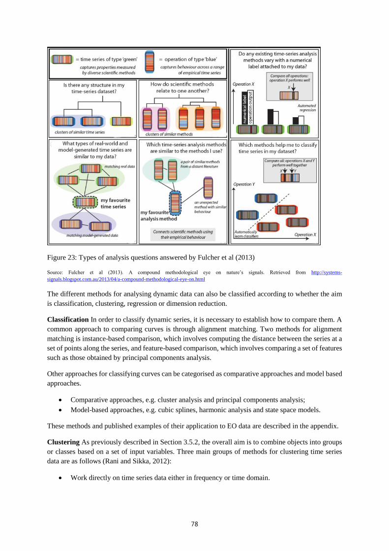
78
Figure 23: Types of analysis questions answered by Fulcher et al (2013)
Source: Fulcher et al (2013). A compound methodological eye on nature’s signals. Retrieved from http://systems-
signals.blogspot.com.au/2013/04/a-compound-methodological-eye-on.html
The different methods for analysing dynamic data can also be classified according to whether the aim
is classification, clustering, regression or dimension reduction.
Classification In order to classify dynamic series, it is necessary to establish how to compare them. A
common approach to comparing curves is through alignment matching. Two methods for alignment
matching is instance-based comparison, which involves computing the distance between the series at a
set of points along the series, and feature-based comparison, which involves comparing a set of features
such as those obtained by principal components analysis.
Other approaches for classifying curves can be categorised as comparative approaches and model based
approaches.
• Comparative approaches, e.g. cluster analysis and principal components analysis;
• Model-based approaches, e.g. cubic splines, harmonic analysis and state space models.
These methods and published examples of their application to EO data are described in the appendix.
Clustering As previously described in Section 3.5.2, the overall aim is to combine objects into groups
or classes based on a set of input variables. Three main groups of methods for clustering time series
data are as follows (Rani and Sikka, 2012):
• Work directly on time series data either in frequency or time domain.

79
The most common similarity measures used for direct comparison of time series include
correlation, distance between data points and information measures. Hierarchical clustering and
k-means methods are then applied to these measures.
• Work indirectly with features extracted from time series.
The most common features extracted from time series data include points identified visually,
via transformations of the data, or via dimension reduction. The most common distance
measure is the Euclidean distance, although Kullback-Liebler and geometric distances are also
used.
• Work with models built from the time series.
The most common time series models include moving average (MA), autoregressive (AR) and
autoregressive moving average (ARMA) models and variants, hidden Markov models (HMM)
and fuzzy set methods.
Regression Time series regression aims to predict a future response based on the response history from
relevant predictors. Two common methods that are used for this purpose are parametric time series
models that capture temporal dynamics are listed above (MA, AR, ARMA and HMM) and
nonparametric convolutional neural networks which are an extension of static neural networks, adapted
to describe data over time.
Another common aim for time series regression is interpolation of missing data within the spatial and
temporal span of the data. For example, cloud cover is a common reason for missing data in EO images.
Splines are widely used for both spatial and temporal interpolation.
Dimension reduction A common approach to dimension reduction of temporal data is principal
components analysis (PCA). This approach is described in the Appendix. An example of PCA applied
to a time series of Enhanced Vegetation Index (EVI) values is described in Potgieter et al (2007). EVI
from 16-day MODIS satellite imagery within the cropping period (i.e. April–November) was
investigated to estimate crop area for wheat, barley, chickpea, and total winter cropped area for a case
study region in North East Australia. The PCA classification method, and others used in the study, were
trained on ground truth data collected from the study region. In this study, principal component analysis
was used to reduce the EVI time series at each pixel from the 23-image sequence into a smaller set of
transformed variables or principal components (PC), which explained 90% or more of the temporal
variability in the series. Overall, PCA correctly classified 98% of pixels as wheat, barley, chickpea or
non-cropping. This example is discussed further in the Appendix.
3.5.4 Choice of method
The choice of method used for analysis of EO data depends on a number of factors:
• The nature and amount of training data
• The amount of calibration (ground-truthed, in-situ) data
• The type of estimates and inferences required
• The availability of software for modelling and analysis
• The expertise of the team performing the modelling and analysis
The following overall statements can be made:
• Empirical methods are useful if there is sufficient training and calibration data, if a model-based
approach is required, and if the assumptions of the models are tenable.

80
• Semi-empirical methods are useful if the conditions for empirical methods are fulfilled and if
there is some expert knowledge about the input variables and system.
• Physics-based methods are useful if there is a deep knowledge about the system under
consideration and/or if there is a lack of calibration or training data.
• Machine Learning models are useful if there are data available to train the models and evaluate
their fit, but there is an inability or unwillingness to make model-based assumptions or develop
physics-based processes.
A review of studies that have compared different statistical and machine learning algorithms for the
analysis of static EO data is provided in the Appendix.
For dynamic EO data analysis, the Australian Bureau of Statistics (ABS) has recommended the use of
state-space models for the analysis of dynamic EO data. See Tam, S-M. (2015). A Statistical
Framework for Analysing Big Data for more information. These are described in the Appendix.
3.6 STEP 3: Evaluation
The considerations to be addressed in the Evaluation step include (1) critical assessment of the results,
(2) assessment of the accuracy of the results, and (3) assessment of other potential biases or concerns
with the results or their interpretation.
3.6.1 Critical assessment of results
As with any statistical analysis, it is essential to critically review the results with respect to whether
they are sensible from both statistical and domain-knowledge perspectives. This is particularly
important with estimates derived from big data or multiple data sources. Evaluations can include:
• Inspection of the overall magnitude of the results, and identification of results that are outside
expected ranges, etc.;
• Inspection of the precision of the estimates, the size of the prediction intervals and other
measures of variability of the results;
• Comparison of the results with other relevant results;
• Evaluation of whether any assumptions in the model or the modelling process have been met.
3.6.2 Accuracy assessment
Accuracy “is a relative measure of the exactness of an estimate and accounts for systematic errors also
referred to as bias. Therefore, an accurate estimate does not systematically over or underestimate the
true value” (FAO 2016, p. 1).
When considering accuracy assessment, it is important to recognise that sampling effort (accuracy and
representativeness of sampled data used for training) as well as the analytical technique(s) utilised play
important roles. These issues have been described above.
Good practice involves reporting details of these processes, as well as details of the model fit, the
accuracy of the estimates or predictions obtained from the model, and quantification of uncertainty of
these estimates and predictions (Olofsson et al., 2014). These issues are now discussed in more detail.
Model assessment
Regardless of the type of model (empirical, semi-empirical, physics-based, machine learning), the
goodness of fit of the model is typically assessed by comparing the estimated or predicted values
obtained from the model with the observed values, if available.

81
Statistical models are typically subjected to further goodness of fit evaluations using criteria such as
AIC, BIC, likelihood ratios for nested models, and traditional hypothesis tests (if available and
applicable). Where possible, estimates obtained from the model are typically compared with the
observed data, using measures such as misclassification rates for categorical responses and mean
squared error of prediction for continuous responses.
Depending on the available data, a typical statistical practice is to define complementary training and
testing datasets by randomly partitioning the original data (for example, randomly splitting the dataset
into a 75% training set and a 25% testing set). A model is then built using the training data, which is
then assessed for accuracy in various ways on the test dataset. For example, for classification models,
misclassification rates and/or positive predictive value (PPV) could be used to assess how well the
training data predict the test data, and hence how well the trained model may be expected to perform
on new, unknown samples.
Another commonly used approach is cross-validation techniques. Cross-validation is often used in
situations where partitioning the data as described above would significantly hamper the training and/or
testing of the model (for example, smaller datasets where partitioning would leave either the test or
training data sample size too small). The idea of cross-validation is to repeat the validation procedure
described above, using different data subsets each time. The measured fit (for example, the
misclassification rate) is then averaged across these repeats to provide a more accurate measure of the
predictive capabilities of the model under investigation. Cross-validation techniques can generally be
classified into two groups: Exhaustive (all possible splits of the data are undertaken – for example leave-
one-out and leave-k-out cross validation) and Non-exhaustive (not every partition of the data is
computed – these cross-validation approaches can be considered approximations to the leave-k-out
cross-validation technique). Which approach is taken often simply comes down to computational
burden.
Accuracy assessment of map data
An example of accuracy assessment practices for EO data analyses is given by the FAO Map Accuracy
Assessment and Area Estimation Practical Guide (FAO, 2016, http://www.fao.org/3/a-i5601e.pdf).
The following information is extracted from the FAO report, pp. 6, 17.
In an accuracy assessment of map data, the map is compared with higher quality data. The higher quality
data, called reference data, is collected through a sample based approach, allowing for a more careful
interpretation of specific areas of the map. The reference data is collected in a consistent manner and is
harmonised with the map data, in order to compare the two classifications. The comparison results in
accuracy measures and adjusted area estimates for each map category. This process is broken down into
four major components: (i) a map, (ii) the sampling design (iii) the response design and (iv) the analysis.

82
Figure 24: The main four steps of an accuracy assessment: Obtaining and finalising the map data,
sampling design, response design and analysis. The symbols show the software that can accomplish
that step: 1 is R, 2 is QGIS, 3 is Excel, and 4 is Collect Earth.
In an analysis step, an error matrix is produced. The error matrix is a cross-tabulation of the class labels
allocated by map and reference data. It is derived as a q x q matrix with q being the number of classes
assessed. The elements show the number of data points which represent a map class i and reference
class j (nij). Usually the map classes are represented in rows and the reference classes in columns. The
diagonal of the matrix contains the correctly classified data points, whereas the cells off the diagonal
show commission and omission errors.
The accuracy measures are derived from the error matrix and reported with their respective confidence
intervals. They include overall accuracy, user’s accuracy and producer’s accuracy. The overall accuracy
is the proportion of area classified correctly, and thus refers to the probability that a randomly selected
location on the map is classified correctly (see equation 3). User’s accuracy is the proportion of the area
classified as class i that is also class i in the reference data (see equation 4). It provides users with the
probability that a particular area of the map of class i is also that class on the ground. Producer’s
accuracy is the proportion of area that is reference class j and is also class j in the map (see equation 5).
It is the probability that class j on the ground is mapped as the same class.

83
For all three accuracy measures, the confidence intervals need to be derived as well. The formula for
the variance are presented in equations 5, 6 and 7 in Olofsson et al. (2014), and the 95% confidence
interval can be calculated by multiplying the square root of the variance by 1.96.
FAO has applied these accuracy assessment steps to measure forest area and forest area change. These
measures are important for countries with reporting requirements to access results based payments for
reducing emissions from deforestation and forest degradation.
Interpretation of accuracy estimates
For map accuracy judgement on the validity of the data depends on the purpose of the map and should
be assessed on a case by case basis. The following discussion is extracted from the FAO (2016) report,
pp. 20, 21.
For example, for land cover change, it is necessary to look at the accuracy of change and not at the
accuracy of two single land cover maps. Even if both land cover maps have high accuracy measures for
a single point in time, it does not provide any information about the accuracy for change classes. A new
change analysis using remote sensing images is necessary rather than comparing maps from different
times.
The overall map accuracy is not always representative of the accuracy of individual classes (GFOI,
2013). High overall map accuracy does not guarantee high accuracy for forest loss. Therefore, both
producer’s and user’s accuracy for all single classes need to be considered.
Additionally total sample size, the number of strata and the allocation of the total sample size to the
strata can favour one accuracy measure over the other. Accuracy is usually higher for stable classes
than for change classes. Furthermore, accuracy is variable in different landscapes. The steps of the
accuracy assessment described in the FAO practical guide need to be considered when assessing
accuracy value.
Reporting accuracy assessment results
Again, extracting from the FAO (2016) report, p. 23:
When reporting the results of accuracy assessment, the report should not only include the estimates of
accuracy assessment, adjusted area and their respective confidence intervals but also the assumptions
implied by several elements of the accuracy assessment. The assumptions can influence the level of
accuracy, and include, but are not limited to:
1. the minimum mapping unit and the spatial assessment unit
2. the sampling design
3. the forest definition
4. the source of reference data
5. the confidence level used for calculating the confidence intervals (typically 95 %).
The estimates always need to be reported with their respective confidence intervals. Additionally, it is
recommended to present the error matrix in terms of estimated area proportions instead of absolute
sample.

84
For details of the practical application of accuracy assessment, see the Global Forest Change (GFC)
example in the FAO Map Accuracy Assessment and Area Estimation Practical Guide 2016.
3.6.3 Other concerns
Other concerns about the results of EO data analyses can include:
• bias in the data used to generate the model estimates.
• assumptions underlying the adopted model.
• influence of the choice of method of estimation of the quantities of interest.
• potential misinterpretation of the results.
• bias of area estimates directly computed from classified images.
The first two points have been addressed earlier in this chapter, and the last point has been discussed
above. The concern about the choice of estimation method is important since it raises the question of
the margin for subjectivity of the results. Given the wide range of image classifiers and analytic
methods, there is a concern that they can be ‘tuned’ to get the ‘right’ results, for example a desired
proportion between classes, and hence that an analyst could choose/tune the algorithm to obtain the
figure that better corresponds to their a priori belief.
Another concern is the accuracy of the bias correction depends on the sample size of the field data used.
A consequence of this is the value added of remote sensing is generally proportional to the effort put
on the field survey, with the exception of some classes for which identification in the image is
particularly reliable.
These issues can be resolved in large part by following good practice guides – see, for example, the
GEOSS guide by Gallego et al. (2008) – and by promoting transparent reporting, open data,open models
and results and replication of results by independent groups.
3.7 Summary
This chapter has described a range of methodologies for analysing EO data. Following a discussion
about the type of estimates that can be obtained from EO data, the focus turned to the three broad steps
of pre-processing the data, techniques for analysing the data, and the critical evaluation of the analysis
results.
A range of references has been provided to indicate the relevance of the methods described and their
practical application to EO data. The areas of application range across agricultural and environmental
statistics to other fields such water quality detection and urban growth. The relevance of these estimates
for the 2030 Sustainable Development Goals is a focus of the chapter, as described in Section 3.2.
References have also been provided for the technical details of the methods described here. Further
details are provided in the Appendix for selected methods.
In addition to providing references, the chapter has also highlighted a case study for each of the three
broad steps. These include details of a practical approach for pre-processing the data (developed and
used by DSITI, Australia, for over a decade), a state space model for analysing time series of remotely
sensed images (recommended by the Australian Bureau of Statistics) and good practice guidelines for
accuracy assessment based on FAO (2016), and GEOSS (2008). More detailed case studies that employ
the methods described in this chapter are presented in Chapter 4.

85

86
4. Pilot Projects and Case Studies
A number of pilot projects were formulated under the umbrella of the Task Team, covering a range of
applications. These projects are aligned with the mission and strategies of the Task Team; to contribute
to the improvement of official statistics through the use of satellite imagery data, as well as supporting
the monitoring of SDGs.
Pilot projects can be considered examples of how the Task Team is working on its four specific
activities:
• Identify reliable and accurate statistical methods for estimating quantities of interest;
• Suggest approaches for collecting representative training and validation data of sufficient
quality;
• Research, develop and implement assessment methods for the proposed models including
measures of accuracy and goodness of fit;
• Establish strategies to reuse and adapt algorithms across topics and to build implementations
for large volumes of data.
Naturally, progress achieved to date is not homogeneous. Pilot projects show different levels of
development. Three of the more mature projects are showcased in this chapter:
Pilot Project 1: Application of satellite imagery data in the production of agricultural statistics,
undertaken by the Australian Bureau of Statistics (ABS).
Pilot Project 2: Study on Skybox Commodity Inventory Assessment, led by UNSD and undertaken
by Google.
Pilot Study 3: Study on the use of satellite images to calculate statistics on land cover and land use,
undertaken by DANE, Colombia.
Each report describes the processing techniques, data sources, selection criteria, and quality issues
associated with data, as well as the analyses and results obtained at the time of this report.
In addition to the pilot projects, five case studies are included in this chapter to complement the Task
Team Pilot Projects. The case studies are as follows:
Case Study 1: an evaluation of the implementation of various machine learning techniques for
analysis of EO data for crop classification, undertaken by the Department of Science
Information Technology and Innovation (DSITI) Australia and Queensland University of
Technology (QUT) Australia.
Case Studies 2 and 3: two published implementations of EO data analyses for estimation of crop
yield.
Case Studies 4 and 5: two fully operational methods developed for the analysis of EO data to derive
official statistics. These have been developed by the National Statistics Office in Canada and
the DSITI in Australia, respectively.

87
4.1 PILOT PROJECT 1: Application of satellite imagery data in the production of
agricultural statistics (Australia)
The Australian Bureau of Statistics Pilot Study for the application of satellite imagery data in the
production of agricultural statistics outlines the outcomes for the study to be: “(…) to assess the
feasibility of statistical methodology for classifying satellite surface reflectance data to crop type and
estimating crop production”. This project was based on an empirical approach. The full paper is
available on request through the Australian Bureau of Statistics (Marley et al 2014).
Data specifications
ABS acquired Landsat 7 imagery data from Geoscience Australia (GA) since this was the active Landsat
satellite collecting data during the period for which they had ground truth data. Since the pilot was
conducted, it would be recommended to use Landsat 8 or Sentinel 2 data as sources. The Landsat
imagery data in the Australian Geoscience Data Cube (AGDC) is stored in one-degree latitude and
longitude tiles. Each tile is approximately 100km x 100km, with each pixel representing a 25m x 25m
area of land. Each pixel has six reflectance measurements associated with it, corresponding to six
distinct bandwidths on the electromagnetic spectrum, namely red, green, blue, near infra-red (NIR),
short-wave infra-red (SWIR) 1 and SWIR 2. Landsat 7 revisits the same area of land, on average every
16 days, meaning that most pixels have a set of six reflectance measurements every 16 days.
ABS acquired satellite imagery data from the AGDC for the 2010-12 calendar years. The Landsat data
was used for crop classification. The extent of missing data in Landsat 7 imagery is a key quality issue,
which is described in 4.1.4. For future projects this issue could be overcome by using Landsat 8 or
Sentinel 2 data. Since there is a significant amount of missing data, a possible line of future research is
to investigate possible methods for adjusting or imputing for the missing data. A possible solution is
the use Model Data Assimilation approaches described in Chapter 2.
Several MODIS data products are available at the Commonwealth Scientific and Industrial Research
Organisation (CSIRO) and those that were of particular interest to the pilot study are listed in Table 6.
Data from the MOD13Q1.005 product was used to investigate the feasibility of crop detection, which
is measuring the presence or absence of crops, regardless of crop type. Product MOD13Q1.005 contains
the Enhanced Vegetation Index (EVI) layer and the two main quality layers of interest; namely, the
pixel reliability layer and Vegetation Index (VI) quality layer.
The EVI is an example of the semi-empirical algorithm type referred to in Chapters 2 and 3, as the
spectral bands used are known for having a relationship with chlorophyll and thus a measure of
photosynthesis in plants, as well as the nearby infrared reflectance peak caused by healthy leaves.
Product Description
MOD09A1.005 500m pixels
8 day composites20
Band 1 to band 7 plus quality layers
MOD09GA.005 500m pixels
Daily
20 Products described as being 8 or 16 day composites indicates that the data provided for each image pixel are the best quality
measurements from an 8 or 16 day period. In these cases, an additional variable is included, specifying the exact day of the year that the data was measured.

88
Band 1 to band 7 plus quality layers
MOD09Q1.005 250m pixels
8 day composites
Band 1 and band 2 (red and NIR)
MOD11A1.005 1000m pixels
Daily
Land surface temperature/emissivity
MOD11A2.005 1000m pixels
8 day composites
Land surface temperature/emissivity
MOD13Q1.005 250m pixels
16 day composites
Vegetation indices (EVI, NDVI) plus quality layers
Table 6: MODIS data products used in the ABS pilot study
Data processing
This investigative pilot study develops various processing techniques to prepare data for use in
accurately classifying satellite imagery as different crop classes and producing quality crop area
statistics. The technical tasks were preparation and exploration of training data for crop type
classification and preparation of training data for crop detection.
Training data is the data used to build classification models; it is the product of integrating satellite
imagery data and ground truth data and matches satellite land surface reflectance measurements to land
cover or land use classes.
Starting with the ground truth dataset from the Queensland Department of Science, Information
Technology and Innovation (DSITI) the technical tasks, the preparation of training data for crop type
classification consisted of two parts. Firstly, determine the field boundaries and secondly, the estimation
of field-level sowing and harvest dates.
Field boundaries were determined around the observed latitude and longitude points, to capture within
field variation. Manual inspection of satellite imagery data and drawing of boundaries using geo-spatial
software was the most accurate and time-efficient means for determining field boundaries for this small
scale feasibility study.
For each pixel within the manually derived field boundaries, the Landsat 7 reflectance measurements
were extracted for all the time points available from 2010 to 2012 using an internally developed R code.
From this integrated dataset, the next task was to determine the sowing and harvest dates that define the
growing season for each field.
The estimation of field-level sowing and harvest dates was as follows;
• Calculate the median pixel-level EVI value for each field, at each observed time point;
• Fit a smoothing spline to the irregular time series of field-level median EVI values; then the
dates associated with the nearest local minima either side of the date when the ground truth data
was observed were labelled as the sowing (left side) and harvesting (right side) dates.
A number of business rules were incorporated for fields for which the ground truth data had insufficient
satellite imagery data (due to missing data, poor quality data and cloud cover) to support confident

89
estimation of sowing and harvest dates. Out of 962 ground truth sites, this automated method
determined the sowing and harvesting dates for 414 sites. These 414 fields only included those with a
seasonal reflectance pattern that showed distinct peaks and troughs. For future studies, the variance of
the fitted spline could be calculated.
To create the final training dataset, these estimated sowing and harvest dates were used to strip down
the intermediate, integrated dataset to only those pixel reflectance measurements that corresponded to
the growing season of the crop that was observed. A second training dataset was also created, which
contained the smoothed median EVI values at regular intervals over the estimated growing season of
each observed field.
Exploratory data analysis was undertaken on the training data to identify suitable covariates that would
enhance the predictive power of a crop classification model, using repeated measures ANOVA on EVI
and other measurements. Repeated measures ANOVA at the pixel level, with random effects for crop
class and field, was conducted to test the variation of reflectance measurements and the EVI between
crop classes (namely, maize, sorghum, barley and wheat). In the absence of random field effects, an
ANOVA analysis showed that mean reflectance measurements were significantly different between
crop types. However, when random field effects were included, these differences dissipated. While
there was significant variation within and between fields, the variation between crops was not
statistically significant.
The strength of relationships between soil and landscape characteristics available in CSIRO’s Soil and
Landscape Grid (SLG) data and EVI values were explored via various visualisation techniques
including density plots, box plots and scatter plots. The visualisations demonstrated there is not enough
evidence to indicate the SLG variables have significant relationships with the satellite reflectance
measurements. Random forests were also considered for variable selection. As a result of this brief
investigation, only a small number of significant relationships were found. For example, wheat crops
require deeper soils with higher levels of clay. However, the results showed the inclusion of the soil
and landscape variables actually increased prediction error; hence this was not considered further.
A number of phenological characteristics were derived from the field-level smoothed EVI curves, to
use in crop classification models, including length of a crop growth cycle in days, number of days taken
to reach maximum EVI since sowing, areas under the curve in different growth phases and within field
EVI distributional measures such as range, maximum, minimum, kurtosis, skewness and variance. A
major limitation of crop growth curve characteristics for statistical modelling is a potential high degree
of multi-collinearity between variables. Multi-collinearity can be overcome by dimension reduction
techniques, such as principal component analysis (PCA). An alternative methodology, functional data
analysis, was also trialled which created functional forms from the entire (smoothed) EVI series for the
growing season. This approach avoided problems in model variable selection of suitable phenological
characteristics and the issue of multi-collinearity.
Next training data was prepared for crop detection. It started with building a crop detection model,
which served to create a crop mask. To create a crop mask, ground truth data containing sites that have
been and have not been used for cropping is required. The north-west region of Victoria was chosen as
the pilot region for this exercise, for which ground truth data was available from the Australian Ground
Cover Reference Sites Database (AGCRDS) and the ABS 2010-11 Agricultural Census.
The ground truth dataset included 18 unique sites in the AGCRSD within the north-west region of
Victoria, and nine sites from the 2010-11 Agricultural Census respondents in the study area. Additional

90
sites that were used for non-cropping land use (such as bodies of water, national parks, forests, etc.)
were required to give balanced ground truth data, and these were selected manually by eye using Google
maps. The bounding latitudes and longitudes of the selected sites were recorded in the ground truth
dataset, along with the crop status and the season; only the year that the ground truth data was collected,
in which the ground truth observation occurred.
Data selection
To satisfy the project purposes, different data sources were included; satellite imagery (mainly MODIS
and Landsat); ground truth data (agricultural census, reference sites and roadside observation data
collected by DSITI). In future work, these datasets may be complemented with additional data sources
such as Sentinel-2, VIIRS, Sentinel-3, Synthetic aperture radar data from Sentinel-1, SLG data, and
meteorological and climate data.
Nevertheless, there is a key issue concerning the availability and suitable quality of EO data sources;
freely and commercially available data have restrictions related to missing values, periodicity and
quality. Two ways to overcome these issues were considered. The first was validation and
standardisation. This involved comparing data from the same source at different times, and/or
comparing between several sources. The AGDC Landsat data for Australia has been pre-processed and
calibrated to the same standard across time. CSIRO’s MODIS data has been similarly standardised,
however other satellite imagery sources would need to be standardised before usage in crop detection
and classification analysis. The second issue was capacity. Even freely available data and tools require
qualified personnel (e.g. data scientists) to properly extract the wealth of information contained in them.
This process may nevertheless be quite resource intensive and needs to be planned for in any Big Data
undertaking.
4.1.4 Quality issues
Missing data was a key quality issue for this pilot project. There are two main sources of the missing
data:
1. Landsat 7 images are plagued with stripes of missing data, caused by a malfunction of the scan
line corrector on board the satellite since May 2003. The stripes are regularly spaced following
the edge of Landsat’s scan and should not be correlated with the type of agriculture grown in
the pixels affected; hence it should not lead to statistical bias except in terms of reducing the
effective sample size. This is not a problem for other satellites, in particular Landsat 8 which
is now in use and retrieving data and Sentinel-2 which is now collecting more frequent data at
10 m resolution.
2. GA supplied a quality layer with the satellite imagery data, treating any pixels labelled as poor
quality as unusable. The main causes of poor quality are cloud cover or cloud shadow. This
approach prevents poor quality pixels affecting results.
There is also significant variation in satellite reflectance patterns between different fields growing the
same crop type. Obtaining additional predictor variables that explain these variations from one area to
another might help improve the classification model’s prediction accuracy, however this has proved to
be a significant hurdle to obtaining more statistically accurate results. This problem is associated with
the empirical approach, but potentially could be overcome by using biophysical approaches which were
not in scope of this pilot project.

91
4.2 PILOT PROJECT 2: Skybox Commodity Inventory Assessment- now part of Planet
(UNSD and Google)
The Google pilot project explored the estimation of crude oil inventory using analytics derived from
satellite imagery as a means to promote economic transparency.
The pilot specifically focused on quantifying volumes of base commodities, namely crude oil, using
satellite imagery. The trade of this commodity, though vital to the global system and central to the
economies of numerous emerging countries, is often inaccessible or inaccurate.
By measuring the shadows on floating lid crude oil tanks, Skybox attempted to assess the volume of
inventory present in a given tank. This was done using fairly straightforward trigonometry, taking into
account the target’s latitude & longitude, the time of day, and the satellite’s collection angle.
To assess the accuracy of the core methodology, Google conducted analysis of the Cushing, Oklahoma,
USA oil storage site. This is the largest oil storage facility in the world, and the EIA conveniently
publishes weekly data on oil inventory stored there. By analysing the difference between Google
estimates and official reporting, one should be able to assess the accuracy of approach.
Data specifications
Panchromatic 450 – 900nm
Blue 450 – 515 nm
Green 515 – 595 nm
Red 605 – 695 nm
NIR 740 – 900 nm
Panchromatic GSD 90 cm at nadir
Multispectral GSD 2 m at nadir
Swath Width 8 km at nadir
File Format 16 – bit Geo TIFF
Table 7: Imagery specifications
Colour Panchromatic
Duration Up to 90 seconds
Frame Rate 30 frames per second
GSD 1.1 m at nadir
FOV 2 km by 1,1 km
File Format MPEG – 4 (H 264
encoding)
Table 8: Video specifications
Data processing
Normal issues such as cloud cover were presented and solved by a combination of human and automated
processing. Further details about data processing techniques were not included due to commercial
sensitivities related to the project.

92
Data selection
Data were adequate to fit the purpose of the project. In this case, a single source has been used; SkyBox
(now Planet) imagery sub-meter accuracy.
The data used by Google focused on monitoring specific targets with high economic importance; the
major refineries, metropolitan areas, mines and maritime ports, among others.
Quality issues
Google used images from Skybox. Regarding the crude inventory assessment, Skybox leveraged a
proprietary combination of fully-automated and human-refined processes. The error in the
measurements is being researched on an ongoing basis, but potential sources include relatively high
solar angle during summer months, image processing methodology, signal to noise ratio, facility and
infrastructure idiosyncrasies, and satellite collection angle.
In some cases there were gaps in collection due to cloud cover. However, with a full constellation of 24
satellites, Skybox will be able to observe any location on earth between five and seven times per day.
This could help significantly to overcome missing data issues.

93
4.3 PILOT PROJECT 3: Use of satellite images to calculate statistics on land cover and
land use (Colombia)
DANE conducted a pilot project with the aim to propose a method to calculate SDG indicator 68 "Ratio
of land consumption rate and population growth rate", and seeks to obtain an estimation of land use
efficiency, through monitoring the relationship between land consumption and population growth
(SDSN, 2016):
“(…) this indicator benchmarks and monitors the relationship between land consumption and
population growth. It informs and enables decision-makers to track and manage urban growth at
multiple scales and enhances their ability to promote land use efficiency. In sum, it ensures that the
SDGs address the wider dimensions of space and land adequately and provides the frame for the
implementation of several other goals, notably health, food security, energy and climate change”.
The objectives of the project were;
• To assess the feasibility of applying remote sensing methods for the estimation of land
consumption rate, and Geographic Information Systems (GIS) based spatial analysis for the
calculation of the relationship between land consumption and population growth in
metropolitan areas;
• To evaluate the methodology by its application to the Barranquilla metropolitan area, through
satellite images and population data for the years 2005, 2010 and 2015.
Data Specifications
To calculate the indicator, the time interval of five years was chosen. This criterion was considered
appropriate to see the evolution in the population and to have adequate imagery coverage. The years
included in the analysis are 2005, 2010 and 2015.
The criteria to choose the images were:
• Availability
• Cloud coverage under 10% of the study area
• Same month for each year to minimise the changes generated by rainy or drought seasons,
phases of crops and others
• Full coverage of the metropolitan area to avoid image mosaics
• Similar spectral bands.
Free Landsat images were used, and were downloaded from the United States Geological Survey
(USGS) Earth Explorer website (http://earthexplorer.usgs.gov/). The study area is covered by the
Landsat path-row 9-52. Table 10 shows mission, date and file name for each image used in the pilot
project.
Path-Row Mission Capture date File
9-52 Landsat 7 January 7 2005 LE70090522005007ASN00
9-52 Landsat 7 February 8 2005 LE70090522005039EDC00
9-52 Landsat 5 January 29 2010 LT50090522010029CHM01
9-52 Landsat 8 January 11 2015 LC80090522015027LGN00
Table 10: Landsat images included in the pilot project
For 2005, two scenes were collected. This was necessary to perform an enhancement on the image. The
process is described in the processing section.

94
Data processing
Processing techniques involved two steps; imagery pre-processing and change detection
(image segmentation and classification). Imagery pre-processing included procedures to prepare
the images for the classification process; filling the gaps (for the year 2005 image), radiometric
resolution scaling (for the year 2015 image), cartographic projection, subset image creation and layer
stacking. To fill the gaps, the USGS Gap-Fill Algorithm was used to improve 2005 images Landsat 7
ETM+ due to lack of Scanning Line Corrector (SLC). A radiometric resolution scaling was carried out
for the 2015 Landsat 8 image.
Subsets of the images were generated covering a buffer of 500 meters around the metropolitan area of
Barranquilla. This distance is a compromise between the coverage of the surrounding areas and the
spatial limitation of the 2010 Landsat 5 image, which is smaller than those from the other missions. The
transition from Landsat 5 to Landsat 7 and then to Landsat 8 included the addition of new bands (layer
stacking) and some previously defined were sub-divided. Even so, most of them are comparable.
The second process carried out was change detection. It was used for post-classification comparison. In
this method, each date of rectified imagery is independently classified to fit a common land type schema
(equal number and type of land-cover classes). The resulting land cover maps are then overlaid and
compared on a pixel-by-pixel basis. The result is a map of land-cover change. This per-pixel comparison
can also be summarised in a ‘from-to’ change matrix, also called a transition matrix. The ‘from-to’
change matrix shows every possible land cover change under the original classification schema.
Image classification is the process used to produce thematic maps from imagery. Since one of the
objectives in the pilot project was to identify urban settlements and given their spectral response is very
similar to that from barren or minimal vegetation, the OBIA method was used in order to include
additional features to the spectral ones and to improve the thematic accuracy. To perform the process,
the open-source INTERIMAGE was used (no license payment). The image to be classified, and the
semantic network (hierarchical entities that will be identified in the image) were entered to
INTERIMAGE as input. Then, the methods and operators that allow the generation of objects and their
classification were defined.
Figure 25 describes the components of the interpretation process on INTERIMAGE. The system
implements a specific interpretation control strategy, guided by a structured knowledge model through
a semantic net (hierarchical entities that will be identified in the image). The interpretation control is
executed by the system core, which uses as input a set of geo-referenced images, SIG layers, digital
elevation data or other geo-registered data. Through the interpretation of the scene, input data are
processed with the help of top-down and bottom-up operators.

95
Figure 25: INTERIMAGE flow chart for object-based classification.
Top-down operators are responsible for the partition of the scene into regions, considered as object
(segmentation). This process creates objects by grouping similar pixels. It starts with each pixel forming
one image object, which is sequentially merged to form bigger ones. The Normalised Difference
Vegetation Index (NDVI) numerical indicator and TA Baatz Segmenter algorithms were used to
obtain the image segmentation.
After defining the segmentation algorithms, decision rules were introduced for each node of the
semantic network. These rules allow filtering, from the set of objects, those that belong to the class of
interest. In a decision rule, it is possible calculate a variety of attributes based on spectral values, shape,
texture and topological characteristics of image segments. These attributes can be used to select objects
within a set, with a user-defined threshold. Objects that are not within a threshold are evaluated in a
different class according to the order defined in the semantic network. If an object meets the criteria for
more than one class, it is assigned to that with the higher reliability.
Top-down operators are responsible for the partition of the scene into regions, considered as object
hypotheses (segmentation). This is a preliminary classification which identifies segments with the
potential to belong to each class. The bottom-up operators refine the classifications produced in the top-
down step (confirming or rejecting) and solving possible spatial conflicts between them. At the end of
the interpretation process, the hypotheses become validated object instances (classification).
The image to be classified, and the semantic network (hierarchical entities that will be identified in the
image) are entered to INTERIMAGE as input. Then, the methods and operators that allow the
generation of objects and their classification are defined.
The project’s semantic net was created based on the previous knowledge of the study area and taking
into account the Landsat imagery land cover classification from the project GeoCover21.
21 http://www.mdafederal.com/geocover

96
Finally, the Normalised Difference Vegetation Index (NDVI) numerical indicator and TA Baatz
Segmenter algorithms were used to obtain the image segmentation
Data selection
Despite some quality issues, the Landsat data was fit for the purposes of the project because it was
freely available and there are several tools to solve quality issues. For future projects using EO data
sources such as Landsat 8 and Sentintel-2 could overcome quality issues associated with Landsat 7
data.
The second source of data was population data. Considering that 2005 was the last year a census was
carried out in Colombia, population projections were used. This could affect the quality of the results,
but is the most common available option to have population information during inter-census periods.
This data source was adequate to meet the project´s goals.
Criteria to select data were related to free availability and opportunity. In this sense, they were
appropriate. A possible search of additional sources can be done in future exercises with MODIS,
Sentinel-2 Landsat 8, Sentinel-3 VIIRS imagery, for instance, and emerging processing tools like
Google Earth Engine.
Quality issues
After using the USGS Gap-Fill Algorithm, the improved Landsat 7 images showed enough quality for
the study purposes. A confusion matrix was calculated using Google Earth images and orthophotos
for reference. This matrix, as mentioned previously in Chapter 3, allows assessment of the
classification quality.
97
4.4 CASE STUDY 1: Application of machine learning techniques to satellite imagery data
in the production of agricultural statistics (Australia)
As an extension of the ABS pilot project for the task team, researchers at the Queensland University of
Technology (QUT) in Australia applied a range of machine learning techniques to the problem of crop
classification, using the same data that were acquired for Pilot Project 1. The aim was to evaluate the
ease of application of the methods and compare the resultant estimates.
The machine learning methods included neural networks, boosted regression trees and regularised
multinomial regression. These methods are described in the Appendix. Two types of regularisation were
used as forms of variable selection, with Ridge regularisation shrinking the coefficients of ineffective
variables substantially, and Lasso regularisation shrinking them to zero and hence effectively
excluding them from the analysis.
Data specifications
This case study used the Landsat data from the ABS pilot project. Data specifications are described in
Section 4.1.1.
The response variable was crop type. The ground truth dataset comprised seventeen (17) crop types:
bare soil, barley, barley, cotton, leucaena, lucerne, maize, millet, mungbean, oats, improved pasture,
natural pasture, peanut, sorghum, forage sorghum, sunflower, wheat and woody vegetation.
The six spectral bands from the Landsat data, as well as the month and year of the observation, were
used to predict the crop type. As no time series method was incorporated here the data set was reduced
to only those months known to have ground truth values (March 2011, September 2011 and February
2012). A ground referenced dataset of land cover categories for 1186 sites was available to construct
and evaluate the models.
Data processing
Ground referenced observations of land cover typically were for areas spanned by multiple pixels of
Landsat 7 imagery. Thus the 1186 ground referenced observations of land cover categories expanded
to 247 210 pixels of satellite imagery. These ground referenced pixels are referred to as observations.
The proportion of pixels corresponding to each crop type in the ground referenced dataset varied widely.
Dominant crop types were cotton (28%), sorghum (22%), natural pasture (13%) and wheat (11%). Nine
(9) crop types had less than 1% of the total number of ground referenced pixels.
An 80/20 training/validation split was used for all analyses (i.e., a random sample of 80% of the ground
referenced observations was used to construct the model and the predictive capability of the model was
then assessed using the remaining 20% of the data). The number of repetitions (runs) with different
training/validation samples varied for the different machine learning methods, and was generally small
because the large volume of data meant that runs were computationally prohibitive and that the variance
in results between runs was minimal.
Various vegetation indices (VIs) were calculated as functions of the Landsat imagery data. As described
earlier in this chapter, VIs are designed to highlight the contrasts between bands that may be indicative
of vegetation characteristics. The functions that define VIs can be more complex than the products and
polynomial terms typically used for covariates in regression analyses. There is a range of software to
calculate VIs from reflectance data; see, for example, the R packages ‘hsdar’ Meyer and Lehnert (2016)
and ‘RStoolbox’ Leutner and Horning (2016). However, given the apparent internal inconsistencies in
the ‘hsdar’ package and the requirement of the ‘RStoolbox’ package of reflectance data in raster format,

98
selected vegetation indices were calculated by hand using the formulae in the RStoolbox package and
constants provided by Ahmadian et al. (2016) and She et al. (2015).
Implementation of Methods
All analyses were undertaken using the R statistical software. The parameters of the neural network and
boosted regression trees were tuned by hand to provide optimal results. The neural network was fitted
using the H2O package with the ‘rectifier’ activation function and hidden layer layout of 200 nodes in
layer 1, 100 nodes in layer 2 and 15 nodes in layer 3. The boosted regression tree was fitted using the
‘gbm’ package. Both ridge and LASSO regularised multinomial logit regression models were fitted
using the R package ‘glmnet’ with 100-fold cross validation. Since cross validation on data with
extremely rare categories is problematic, the regression models were restricted crops with at least
10,000 observations (bare soil, cotton, maize, natural pasture, peanut, sorghum and wheat).
For the regression methods, since there was considerable collinearity among the original imagery bands
and vegetation indices, the design matrix was filtered to enforce a maximum correlation coefficient
magnitude between remaining covariates of 0.85. The retained variables were Landsat bands 1, 3, 4 and
5, the Normalised Difference Vegetation Index (NDVI), Soil Adjusted Vegetation Index, Modified
Normalised Difference Water Index (MDWI) and Simple Ratio Vegetation Index (SR). All covariates
were re-centred and re-scaled (to column means of zero and column Ll norms of one). Linear, pairwise
interactions and polynomial terms up to polynomial order four were included in the regression models.
Two different approaches were used to assess the results, namely a confusion matrix and a Receiver
Operating Characteristic (ROC) curve. In the confusion matrix, the predicted crop classes are compared
with the actual classes. The ROC shows the correct classification rate of a binary classifier as the
discrimination threshold is varied.
Results
The neural network configuration resulted in an overall misclassification rate of approximately 26%
averaged over 10 iterations. The variance for these iterations was less than 8.3e-06. However, the
misclassification rates for specific classes were far worse. There was a fairly clear correlation between
the accuracy for a given class the overall proportion of that class in the sample. One potential method
to address this would be to use a more even sample distribution by class which is non representative of
the true ratios. Alternatively, a small proportion of classes could be dropped or combined into a single
‘other’ class.
The boosted regression tree approach revealed the domination of one variable, band 5 of the Landsat
imagery, in discriminating between the crop types. The relative influence of this band compared with
the other five bands is shown below. Band 5 (1.55 - 1.75u m) is sensitive to the turgidity or the amount
of water in plants. In other environmental studies band 5 has separated forest lands, croplands, and
water bodies. Forests have appeared as a comparatively darker tone than croplands (light grey) and
grass lands (lighter tone). No improvement was gained by including the derived vegetation indices. It
is likely that any complex relationship captured by a pre-processed VI could be similarly represented
by the original variables in the boosted regression tree analysis and therefore adds little value.

99
Figure 26: Relative influence of Landsat imagery bands, obtained from the boosted regression tree
analysis.
The Lasso regularised multinomial logistic regression models were able to correctly categorise 78% of
the Landsat pixels. The nonlinear and interaction terms contributed less than half a percent to overall
classification accuracy, but they improved the classification of particular crop types. For example, under
the Lasso models the inclusion of these terms provided much better classification of maize.
The Ridge models achieved an overall correct classification rate of 68.5% using only linear effects. In
contrast to the Lasso models, the Ridge models assigned no pixels to maize and very few to wheat, and
were also substantially less accurate in classifying peanut and natural pasture. The addition of nonlinear
and interaction terms increased the overall correct classification to 75%, with substantial improvement
in classification of wheat, maize and peanut. In contrast to the Lasso models which by construction
eliminates uninformative variables, all covariate terms are retained in the Ridge models.
Discussion
This study achieved its aim to implement a range of machine learning methods for analysis of EO data.
For all methods, there were challenges in managing large datasets and correctly classifying a large
number of crop types, some of which are very small. While the methods are readily available in software
such as R, these challenges meant that considerable time and effort was required to implement and tune
the methods. Nonetheless, the study confirmed the conclusions of other published papers, that these
methods hold great promise for automatic crop type identification.
Some improvements to the implementation of the methods were noted. First, in the current analysis the
cross validation folds were constructed by random subsetting of the full data set using the default
method supplied in the ‘glmnet’ package. A better strategy would be to use a set of folds constructed to
ensure that each fold contains approximately the same proportion of observations of the different
response categories as are present in the complete data. Second, the challenge of identifying rare
responses could be better addressed by artificially inflating the number of observations in these
categories using bootstrapping or subsampling techniques, or by enforcing different degrees of
coefficient shrinkage for the various response categories. Third, additional model diagnostics could
assist in better understanding the misclassification rates for different crop categories and hence reducing
them. Fourth, additional covariates could be considered, such as MODIS derived variables and tasselled
cap indices. Fifth and last, other regularisation methods for the regression models, such as elastic net,
could be evaluated, taking into account the different computational burdens.

100
4.5 CASE STUDY 2: Crop yield prediction (USA)
This study, reported by Gao et al (2017), aimed to derive crop growth stage and predict yield from
remotely sensed data, to contribute to more efficient management of irrigation, improved food security
and efficient commodity trading.
The EO data were intended to supplement ground based observation on crop progress and condition
currently published by USDA NASS. Under this system, reporters provide visual observations and
subjective estimates of crop progress, which are published weekly in the NASS Crop Progress reports.
Gao et al extend the application of data fusion down to sub-field scales for phenology mapping over
agricultural landscapes. The main objective was to test the ability of this Landsat-MODIS data fusion
methodology to map crop phenology at 30-m resolution, where crop growth stages for different crops
can be distinguished. Maps of crop progress were produced across an intensively cropped area in central
Iowa.
Data specifications
The study area was in central Iowa, in a rain-fed agricultural area in the U.S. Corn Belt region. Corn
and soybean are the major crop types.
Nine years of Landsat and MODIS data from 2001 to 2014 were chosen to generate the fused Landsat-
MODIS reflectance time-series for crop phenology mapping.
Other data sources included in the study are briefly summarised here:
• The cropland data layer (CDL). NASS CDL 30-m resolution data from 2001 to 2014 were
downloaded and used to analyse the crop phenology patterns for major crop types over the
study area.
• Flux tower data. In-situ meteorological and surface flux measurements were collected over a
pair of adjacent agricultural fields north of Ames (near Buckeye), IA in Hardin County.
• Field biophysical data. Field observations of crop progress were conducted during growing
seasons from 2010 to 2013, sampling two observation sites in Dallas County, Iowa located
within the study area.
Data processing
The analyses conducted in this study include two core components: data fusion and phenology
extraction. The entire processing flow chart is shown below. For further details see Gao et al (2017).

101
Crop phenology data processing and analysis flow chart. Rectangles indicate data products and ellipses
represent processing steps/modules
Source: Gao et al (2017). Toward mapping crop progress at field scales through fusion of Landsat and
MODIS imagery. Retrieved from:
http://www.sciencedirect.com/science/article/pii/S0034425716304369
Data selection
Only mostly clear Landsat scenes were used as fine resolution images to pair with MODIS data as input
to STARFM. Partially clear Landsat images were not used in the data fusion process. Landsat 7 images
that suffer SLC failure after May 2003 were not used as input pair images since SLC-off gaps will
remain in the fused images and affect the subsequent phenology mapping. However, all valid and clear
pixels (as identified in the cloud mask) from all available Landsat images, including partially clear and
Landsat 7 SLC-off images, were used in the phenology mapping itself.
Method
The STARFM approach was used to produce multi-year daily 30-m surface reflectance and NDVI time-
series which captured spatial and seasonal variability between the corn, soybean and forested vegetation
classes that characterise this region. The STARFM data fusion approach has been described in detail in
Gao et al. (2006).

102
Two approaches (MODIS and TIMESAT) were applied to extract crop phenology from the daily time-
series NDVI. The TIMESAT approach relies on a pre-defined threshold (percent change of the seasonal
amplitude between minimum and maximum NDVI values) to determine the start of the season, the end
of the season, and the length of the season. The MODIS phenology approach uses curvature analyses
to identify inflection points in the fitting curve. A double logistic function was selected to fit time-series
NDVI for both approaches.
Crop phenology metrics retrieved from the fused Landsat-MODIS data were compared to crop growth
stages reported at district and county levels from the NASS CP reports. Observations at the field scale
were examined using the corresponding Landsat pixels.
The figure below shows the fitted NDVI curves from 2011 for corn and soybean pixels at the two South
Fork flux tower sites, overlaid with the crop growth stages from NASS county-level CP reports. Also
shown are daily NEE and GPP estimates derived from eddy covariance measurements during the
growing season in 2011. The general correspondence in the time behaviour of the NDVI and crop
carbon uptake curves demonstrates that the NDVI time-series appears to be behaving reasonably in
these two fields in relationship with the NASS CP stages.
Figure 27: NDVI curves for corn (a) and soybean (b) pixels compared to daily NEE and GPP (secondary
axis, only measured during vegetative growing season) and crop growth stages from NASS county-
level reports in 2011 (red vertical lines). Clear correspondences can be identified among time-series
NDVI, NEE and GPP during crop vegetative stages at the Landsat pixel resolution.

103
Source: Gao et al (2017). Toward mapping crop progress at field scales through fusion of Landsat and MODIS imagery. Retrieved from:
http://www.sciencedirect.com/science/article/pii/S0034425716304369
Quality issues
Application of these methods in real-time is another area that requires additional research.
Operationally, crop growth stages and conditions need to be reported weekly throughout the current
growing season. The phenology programs used in this paper were not designed to map within-season
crop phenology using partial years of data. However, the growth-shape model approach of Sakamoto
et al., 2010 and Sakamoto et al., 2011 may be adaptable for real-time field-scale applications using
fused Landsat-MODIS time series.
Results
The STARFM approach was used to produce multi-year daily 30-m surface reflectance and NDVI time-
series which captured spatial and seasonal variability between the corn, soybean and forested vegetation
classes that characterise this region. Biases between fused and observed Normalized Difference
Vegetation Index (NDVI) were between − 0.011 to 0.028 and mean absolute differences were < 0.083
for all years from 2001 to 2014. These biases are due in part to sensor, waveband, and view angle
differences between Landsat and MODIS acquisitions, and it was demonstrated that it is important to
characterise these biases to fully understand performance of the fusion output.
Using time-series of 30-m resolution NDVI maps derived from Landsat-MODIS data fusion, crop
phenological metrics were extracted using two established phenology programs (MODIS and
TIMESAT). While both approaches generated comparable metrics, the MODIS curvature approach was
deemed most practical for operational applications because it does not necessitate specification of pre-
defined thresholds, as required by the TIMESAT approach.
The results of the study suggest there is utility for robustly backcasting emergence from remote sensing,
e.g. as input to crop simulation models. This study demonstrated that time-series data from multiple
remote sensing sources can be effectively integrated and used to detect major crop physiological stages
at the field scale. At 30-m resolution, the phenology for corn and soybean crops can be clearly separated
and quantified for field sizes typical in the United States. This capability has applications in farmland
management and yield prediction. However, routine mapping of crop growth stages within the season
is still challenging due to the fact that only a partial year of data is available for near real-time mapping.
Real-time applications will require an appropriate phenology approach and frequent clear-sky remote
sensing imagery. Satellite image data fusion can play a significant role in achieving this goal.

104
4.6 CASE STUDY 3: Monitoring crop development (South Korea)
The aim of this study was to investigate the applicability of high-temporal-resolution Geostationary
Ocean Colour Imagery (GOCI) satellite data for monitoring the development of paddy rice in South
Korea. The monitoring measures included spectral analyses and vegetation index profiles. GOCI
launched successfully on 27 June 2010. It is designed to detect, monitor, and predict regional ocean
phenomena around Korea and is equipped with eight spectral bands (six visible, two near infrared).
Data specifications
In this study, two paddy rice areas were selected; one was located in Kyehwa and corresponds to a
GOCI pixel with coordinates of 35°46′37N and 126°41′03E (Figure 1b). The other was in Kimjae and
corresponds to a GOCI pixel with coordinates of 35°44′59N and 126°52′15E (Figure 1c).
The study site at Kimjae represents the double cropping of barley and early maturing rice cultivars, and
the site in Kyehwa represents the most popular paddy rice agriculture with an intermediate-late-
maturing rice cultivar. As these study sites are relatively homogeneous, despite the small paddy units,
the temporal dynamics of different crops should be recognisable in the daily satellite image data
analysis.
Figure 28: Study area. (a) Red Green Blue (RGB) colour composite image from the Geostationary
Ocean Colour Imager (GOCI) acquired on 1 April 2011. The red rectangles, (b) and (c), in (a) are shown
in (b), and (c), respectively, giving detailed views using high-resolution RapidEye multispectral data
obtained on 5 August 2011 (b), and 11 October 2011 (c). The blue rectangles in (b), and (c) are
geometrically matched with corresponding satellite observation pixels.
Source: Yeom, J-M., and Kim, H-O. (2015) Comparison of NDVIs from GOCI and MODIS Data towards Improved Assessment of Crop
Temporal Dynamics in the Case of Paddy Rice. Remote sensing (7), 11326 – 11343.

105
Ground measurements were performed using the multispectral radiometer (MSR) to evaluate satellite-
based vegetation profiles for comparative analysis. Field measurements were carried out from June to
October 2014. To obtain the crop development characteristics of the paddy rice, measurements were
made on eight dates based on the cultivation schedule, including transplantation and harvest.
Data processing
For the GOCI satellite image, further pre-processing, including conversion of digital numbers (DN) to
radiance, cloud masking, and atmospheric correction, was performed to calculate surface reflectance.
See Yeom and Kim (2015) for further details.
Data selection
The study compared two sets of optical earth observation satellite data with the same spatial resolution
of 500 m; one was from a geostationary (GOCI) and the other from a sun-synchronous satellite
(MODIS). The fifth and eighth GOCI bands were used for calculating the normalised difference
vegetation index (NDVI). For comparison, MODIS NDVI products were applied as a reference. This
study analysed the data for the years 2011 to 2014.
Quality issues
For the comparison of the NDVI calculated using moderate-resolution satellite data with the field
measurements, it is necessary to consider the mixed-pixel problem. Because the paddy units in South
Korea are relatively very small, it is very difficult to observe a non-mixed spectral value for rice paddies
on the moderate spatial resolution GOCI data.
Method
A vegetation index was calculated from GOCI data based on the bidirectional reflectance distribution
function (BRDF)-adjusted reflectance, which was then used to visually analyse the seasonal crop
dynamics. These vegetation indices were then compared with those calculated using the Moderate-
resolution Imaging Spectroradiometer (MODIS)-normalised difference vegetation index (NDVI) based
on Nadir BRDF-adjusted reflectance.
Results
The results show clear advantages of GOCI, which provided four times better temporal resolution than
the combined MODIS sensors, interpreting subtle characteristics of the vegetation development. In
general, GOCI and MODIS displayed similar temporal variation in NDVI under benign weather
conditions, because they can secure enough cloud-free observations for full inversion BRDF modelling.
During the monsoon season, however, with its long periods of rain and many cloudy days, GOCI was
found to be more useful for extracting cloudless or less cloudy areas by arraying its eight images to
calculate representative daily data.
The study also found the GOCI BAR NDVI was more useful for crop signal monitoring than the widely
used MVC NDVI. The authors concluded the very high temporal resolution of GOCI is very beneficial
for monitoring crop development, and has potential for providing improved information on phenology.
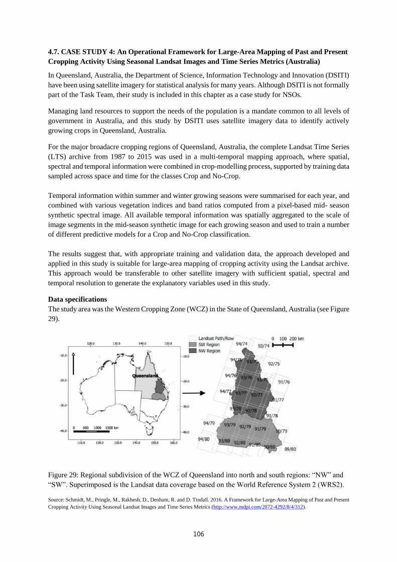
106
4.7. CASE STUDY 4: An Operational Framework for Large-Area Mapping of Past and Present
Cropping Activity Using Seasonal Landsat Images and Time Series Metrics (Australia)
In Queensland, Australia, the Department of Science, Information Technology and Innovation (DSITI)
have been using satellite imagery for statistical analysis for many years. Although DSITI is not formally
part of the Task Team, their study is included in this chapter as a case study for NSOs.
Managing land resources to support the needs of the population is a mandate common to all levels of
government in Australia, and this study by DSITI uses satellite imagery data to identify actively
growing crops in Queensland, Australia.
For the major broadacre cropping regions of Queensland, Australia, the complete Landsat Time Series
(LTS) archive from 1987 to 2015 was used in a multi-temporal mapping approach, where spatial,
spectral and temporal information were combined in crop-modelling process, supported by training data
sampled across space and time for the classes Crop and No-Crop.
Temporal information within summer and winter growing seasons were summarised for each year, and
combined with various vegetation indices and band ratios computed from a pixel-based mid- season
synthetic spectral image. All available temporal information was spatially aggregated to the scale of
image segments in the mid-season synthetic image for each growing season and used to train a number
of different predictive models for a Crop and No-Crop classification.
The results suggest that, with appropriate training and validation data, the approach developed and
applied in this study is suitable for large-area mapping of cropping activity using the Landsat archive.
This approach would be transferable to other satellite imagery with sufficient spatial, spectral and
temporal resolution to generate the explanatory variables used in this study.
Data specifications
The study area was the Western Cropping Zone (WCZ) in the State of Queensland, Australia (see Figure
29).
Figure 29: Regional subdivision of the WCZ of Queensland into north and south regions: “NW” and
“SW”. Superimposed is the Landsat data coverage based on the World Reference System 2 (WRS2).
Source: Schmidt, M., Pringle, M., Rakhesh, D., Denham, R. and D. Tindall. 2016. A Framework for Large-Area Mapping of Past and Present
Cropping Activity Using Seasonal Landsat Images and Time Series Metrics (http://www.mdpi.com/2072-4292/8/4/312).

107
All available Landsat 5 TM, Landsat 7 ETM+ and Landsat 8 OLI data across 27 footprints with cloud
cover of less than 60% were used. This criterion was chosen to reduce the potential for noise in the data
due to imperfect cloud/cloud shadow masking and water vapour variations.
All images were cloud-masked with a regionally adapted version of Fmask22 then NBAR-corrected23;
this latter step converts the units of the imagery to bottom-of-atmosphere reflectance, scaled to the
interval (0, 1). The high internal geometric consistency of the USGS-based Landsat imagery allows
further data processing and analysis without further geometric adjustment.
Data processing
All archived images were used to generate a synthetic spectral image for each season and year. These
images were generated per pixel and per spectral band, excluding the thermal band, based on a statistical
model. Figure 30 provides an example contrived to demonstrate, for a single pixel, how synthetic
reflectance values for a Landsat band were generated for the midpoint of a growing season, t0, within
a particular year. Outliers were Winsorised, then the 4 nearest neighbours to t0 were used in a linear
regression to predict reflectance at t0. For further details see Schmidt et al (2016).
Figure 30: Example of synthetic reflectance value generation process Source: Schmidt, M., Pringle, M., Rakhesh, D., Denham, R. and D. Tindall. 2016. A Framework for Large-Area Mapping of Past and
Present Cropping Activity Using Seasonal Landsat Images and Time Series Metrics (http://www.mdpi.com/2072-4292/8/4/312).
The most recent Queensland Land Use Mapping Program (QLUMP) mapping was used to mask areas
from each synthetic image that were associated with land uses that were not of interest for this study,
such as conservation areas, forestry and intensive uses. Water bodies and travelling stock routes were
also masked for each synthetic image.
22 Flood, N. Continuity of Reflectance Data between Landsat-7 ETM+ and Landsat-8 OLI, for Both Top-of-Atmosphere and Surface
Reflectance: A Study in the Australian Landscape. Remote Sens. 2014, 6, 7952–7970.
Frantz, D.; Roder, A.; Udelhoven, T.; Schmidt, M. Enhancing the Detectability of Clouds and Their Shadows
in Multitemporal Dryland Landsat Imagery: Extending Fmask. IEEE Geosci. Remote Sens. Lett. 2015, 12, 1242–1246.
Zhu, Z.; Woodcock, C.E. Object-based cloud and cloud shadow detection in Landsat imagery. Remote Sens. Environ. 2012, 118, 83–94. 23 Flood, N. Continuity of Reflectance Data between Landsat-7 ETM+ and Landsat-8 OLI, for Both Top-of-Atmosphere and Surface
Reflectance: A Study in the Australian Landscape. Remote Sens. 2014, 6, 7952–7970.
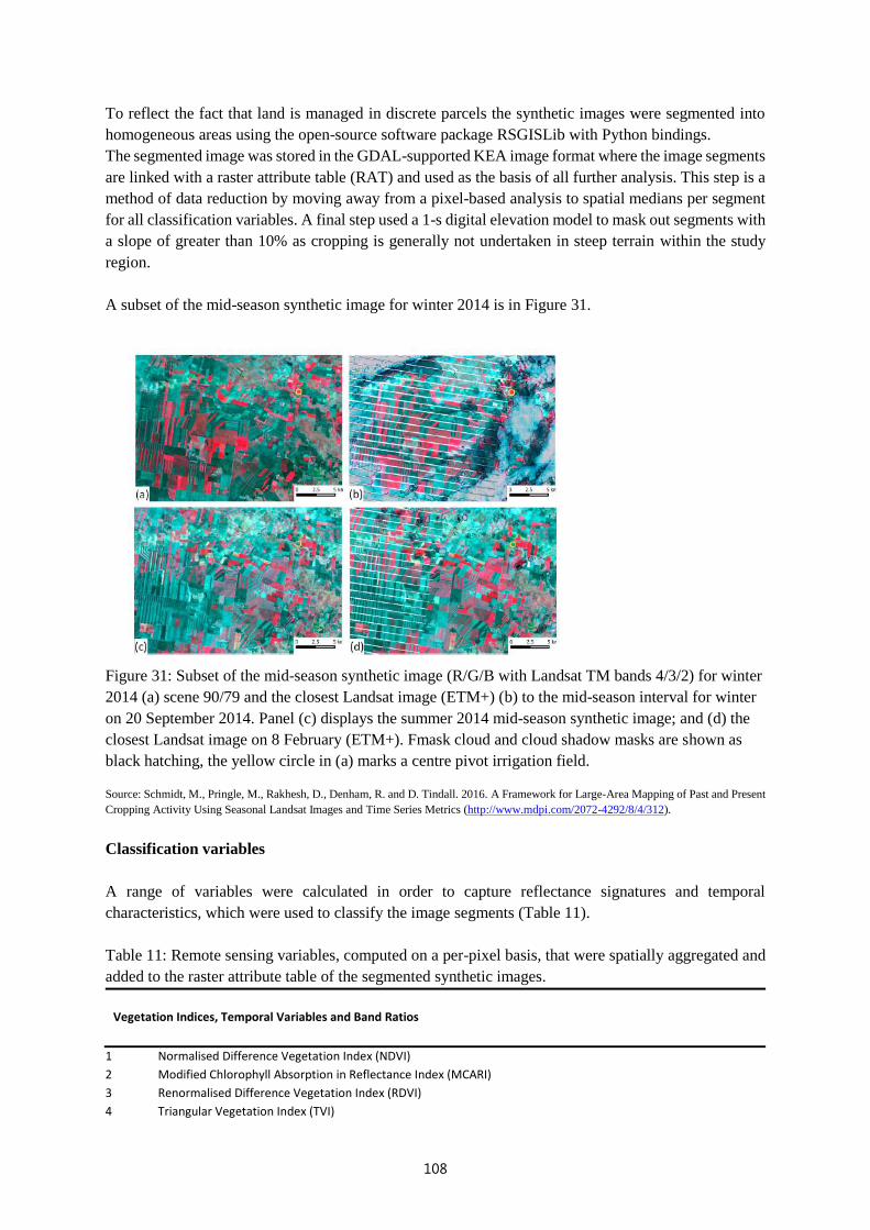
108
To reflect the fact that land is managed in discrete parcels the synthetic images were segmented into
homogeneous areas using the open-source software package RSGISLib with Python bindings.
The segmented image was stored in the GDAL-supported KEA image format where the image segments
are linked with a raster attribute table (RAT) and used as the basis of all further analysis. This step is a
method of data reduction by moving away from a pixel-based analysis to spatial medians per segment
for all classification variables. A final step used a 1-s digital elevation model to mask out segments with
a slope of greater than 10% as cropping is generally not undertaken in steep terrain within the study
region.
A subset of the mid-season synthetic image for winter 2014 is in Figure 31.
Figure 31: Subset of the mid-season synthetic image (R/G/B with Landsat TM bands 4/3/2) for winter
2014 (a) scene 90/79 and the closest Landsat image (ETM+) (b) to the mid-season interval for winter
on 20 September 2014. Panel (c) displays the summer 2014 mid-season synthetic image; and (d) the
closest Landsat image on 8 February (ETM+). Fmask cloud and cloud shadow masks are shown as
black hatching, the yellow circle in (a) marks a centre pivot irrigation field.
Source: Schmidt, M., Pringle, M., Rakhesh, D., Denham, R. and D. Tindall. 2016. A Framework for Large-Area Mapping of Past and Present
Cropping Activity Using Seasonal Landsat Images and Time Series Metrics (http://www.mdpi.com/2072-4292/8/4/312).
Classification variables
A range of variables were calculated in order to capture reflectance signatures and temporal
characteristics, which were used to classify the image segments (Table 11).
Table 11: Remote sensing variables, computed on a per-pixel basis, that were spatially aggregated and
added to the raster attribute table of the segmented synthetic images.
Vegetation Indices, Temporal Variables and Band Ratios
1 Normalised Difference Vegetation Index (NDVI)
2 Modified Chlorophyll Absorption in Reflectance Index (MCARI)
3 Renormalised Difference Vegetation Index (RDVI)
4 Triangular Vegetation Index (TVI)

109
5 Modified Simple Ratio (MSR)
6 Normalised Difference Burn Ratio (NDBR)
7 NDVI seasonal variance (ndviTsVr)
8 NDVI seasonal minimum (ndviTsMn)
9 NDVI seasonal maximum (ndviTsMx)
10 NDVI seasonal coefficient of variation (ndviTsCV)
11 NDVI seasonal range (ndviTsRng)
12 NDVI gradient up (first minimum to maximum) (ndviTsGr1)
13 NDVI gradient down (maximum to second minimum) (ndviTsGr2)
14 NDVI day of time series maximum (ndviTsDyMx)
15 b7 _ b3/(b7 + b3) (nr73)
16 b7 _ b2/(b7 + b2) (nr72)
17 b5 _ b7/(b5 + b7) (nr57)
18 b4 _ b5/(b4 + b5) (nr45)
19 b5 _ b3/(b5 + b3) (nr53)
20 b5 _ b2/(b5 + b2) (nr52)
21 b4 _ b2/(b4 + b2) (nr42)
22 b2/b3 (r23)
23 b4/b3 (r43)
Source: Schmidt, M., Pringle, M., Rakhesh, D., Denham, R. and D. Tindall. 2016. A Framework for Large-Area Mapping of Past and Present
Cropping Activity Using Seasonal Landsat Images and Time Series Metrics (http://www.mdpi.com/2072-4292/8/4/312).
Field-based training data, collected between September 1999 and February 2012, were used in the
study. All records were recoded as either Crop or No-Crop. An additional set of records were generated
through desktop interpretation of seasonal synthetic images sampled at random over space, growing
season and years.
Four classification algorithms were applied to the same training data; SVM, multinomial logistic
regression, decision-tree classifier and RF, all implemented with the R software. Validation revealed
that the predictive accuracy varied by growing season and region and a random forest classifier
performed best, with K = 0.88 to 0.91 for the summer growing season and K = 0.91 to 0.97 for the winter
growing season, and are thus suitable for mapping current and historic cropping activity.
Data selection
All available Landsat 5 TM, Landsat 7 ETM+ and Landsat 8 OLI data since 1987 across 27 footprints
with cloud cover of less than 60% were used. For the majority of seasons there are 10 or more Landsat
images with less than 60% cloud cover. This threshold was applied to reduce the risk of image artefacts
from imperfect cloud and cloud-shadow masking, thin undetected clouds and water vapour variations
which can influence an individual pixel’s reflectance values. High levels of cloud cover also impacted
the geometric accuracy of Landsat 5 data. The data were fit for purpose for the study.
Quality issues
A relatively minor issue is the image segments for the cropped field may not always be sharp on the
field boundaries so some discrepancies with the true field outlines are apparent. Also, the comparison
of the mid-season synthetic image is effective if the crops are greening-up during the particular time,
but if the crop is planted late it might not appear green in the synthetic image. This could lead to
misclassification of segments as no crop in some cases.

110
Recently, the authors have used a similar framework and expanded the mapping approach to broad crop
types (Pingle et al, 2018). This approach includes all available Landsat imagery dating back to 1987
until current, and incorporates additionally Sentinel-2 imagery (from 2015 onwards). In case of large
temporal gaps where also MODIS imagery used as a backup option. In this updated approach a temporal
adaptive seasonal image composite at the time of the maximum EVI was used as input for GEOBIA,
followed by a tree based image classification algorithm of phenological metrcis. The crop types of (i)
Cereal crop (wheat, barley, oats), and (ii) Pulse crop (chickpea) for winter, as well as (i) Coarse-grain
& Pulse (sorghum, maize, mungbean, soybean), and (ii) Cotton crop for summer were compared with
values of official statistics (Figure 32).
Figure 32: The area devoted to the different groups in each growing season, as predicted by the DSITI
model (lines). When available, independent Queensland-wide values are presented (points). The solid
line is the total for the entire study region; the broken line is the total associated soley with a land-use
cropping.
Source: Pringle, M., Schmidt, M. and Tindall, D. (2018): Multi season, multi sensor time series modelling based on geostatistical concepts -
to predict broad groups of crops. Submitted to Remote Sensing of Environment.
For the summer cropping season appears to be an excellent correspondence between state-wide
averages of the crop type maps and official commodities data (ABARES, 2016). The over-prediction
of of the class 'Cereal' seem to be a similar to the under-predction of the class 'Pulse'. The authors have
found little difference between the crop-related summations for their study region.
4.8 CASE STUDY 5: An Operational Approach to Integrated Crop Yield Modelling Using
Remote Sensing, Agroclimatic Data and Survey Data (Canada)
Statistics Canada is an NSO which has used remote sensing data since the early 1980s for applications
such as census and survey validation, crop mapping and area estimation and support program
development. In 2016 they became the first NSO to replace a statistical survey with a remote sensing
model-based approach. The goal of the model was to produce a preliminary estimate of the expected
harvest yield of the crops in late summer using information from existing data sources.
Although Statistics Canada did not produce a pilot project as part of the Task Team, their case study is
included as an example of an NSO using EO data to produce official statistics in practice.

111
Statistics Canada investigated the use of remote sensing, agroclimatic and survey data to model reliable
crop yield estimates as a preliminary estimate to the November Farm Survey estimates, an occasion of
the Crop Reporting Series at Statistics Canada.
Initially these estimates were made available before the September Farm Survey estimates were
released. However, since 2016 the farm survey has not been conducted and only the model based
estimates are published. The process prior to 2016 is described in this case study to demonstrate the
process Statistics Canada used to achieve replacing survey collected estimates with model based
estimates. The work was completed by the Remote Sensing and Geospatial Analysis Section,
Agriculture Division, and by the Business Survey Methods Division at Statistics Canada in
collaboration with Agriculture and Agri-Food Canada (AAFC).
Data specifications
A methodology for modelling crop yield was developed and tested on the crops that are typically
published at the provincial and national levels by the September Farm Survey, as shown in Table 12.
The five provinces listed account for approximately 98% of the agricultural land in Canada, across a
diverse range of climate zones and soil types. The crops that account for approximately 85% of the
revenue for the 19 crops listed are referred to as the seven major crops.
Source: Statistics Canada (2015). Integrated Crop Yield Modelling Using Remote Sensing, Agroclimatic Data and Survey Data. Retrieved
from: http://www23.statcan.gc.ca/imdb-bmdi/document/5225_D1_T9_V1-eng.htm
Table 12: Crops typically published in the results of the September Farm Survey, by province
Table summary
Crops typically published in the results of the September Farm Survey. The information is grouped
by Crop type (appearing as row headers), Province (appearing as column headers).
Crop type Province
Quebec Ontario Manitoba Saskatchewan Alberta
7 major crops
Barley X X X X X
Canola X X X X X
Corn for grain X X X
Durum wheat X X
Oats X X X X X
Soybeans X X X
Spring wheat X X X X X
12 additional crops
Canary seed X
Chickpeas X X
Coloured beans X X
Fall rye X X X X
Field peas X X X
Flaxseed X X X
Lentils X
Mixed grains X X X X X
Mustard seed X X
Sunflower seed X
White beans X X
Winter wheat X X X X X
Note: Fodder corn is typically published in the September Farm survey. However, it was not
modelled due to a lack of July Farm Survey yield estimates.

112
The modelling methodology used three data sources: 1) the coarse resolution satellite data used as part
of Statistics Canada’s Crop Condition Assessment Program; 2) Statistics Canada’s Crop Reporting
Series data, and 3) agroclimatic data for the agricultural regions of Canada.
Data processing
Normalised Difference Vegetation Index (NDVI)
A spectral vegetation index, the NDVI, was used as a surrogate for photosynthetic potential. NDVI is
the normalised ratio of the Near-Infrared (NIR) to Red (R) reflectance (NDVI = (ρNIR − ρR)/(ρNIR +
ρR)) and varies from −1 to 1, with values close to one indicating high vegetation content and values
close to zero indicating no vegetation over bare ground.
The NDVI data were processed on a continuous basis throughout the agricultural growing season (April
to October) for the entire land mass of Canada. Statistics Canada has a time series of NDVI data from
1987 to present, which includes years of severe drought and record production. The daily NDVI images
were processed into seven-day composites as described by Latifovic et al. (2005) and the methodology
was further refined by Statistics Canada to minimise or eliminate NDVI errors introduced by the
presence of clouds (Bédard 2010).
Cropland NDVI statistics by census agricultural region (CAR) were computed and stored in a relational
database for each weekly NDVI composite. Only NDVI picture elements, or pixels, that geographically
coincide with an agriculture land cover database produced by AAFC as part of an annual crop inventory
were extracted to generate the mean NDVI value for cropland within each of the CARs. The agriculture
land cover file and the associated metadata file produced by AAFC were accessible at
www.geobase.ca/geobase/en/data/landcover/index.html.
After the mean NDVI values were computed they were imported as one of the input variable databases
to the crop models as three-week moving averages from week 18 to 36 (May to August).
Survey area and yield data
Statistics Canada’s Field Crop Reporting Series surveys were another dataset used in the model. These
surveys obtain information on grains and other field crops stored on farms (March, July, September and
December Farm Surveys), seeded area (March, June, July, September and November Farm Surveys),
harvested area, expected yield and production of field crops (July, September and November Farm
Surveys). These data provide accurate and timely estimates of seeding intentions, seeded and harvested
area, production, yield and farm stocks of the principal field crops in Canada at the provincial level.
For abundant crops, CAR level crop yield estimates from the July and November Farm Surveys from
1987 to present were used as input variables for the models while yield estimates from the September
Farm Survey and the November Farm Survey were used to verify the accuracy of the yield model
results. For less abundant crops, the survey data were compiled at the provincial level.
Agroclimatic indexes
The climate data collected during the growing season were the third data source used for modelling
crop yields. The station-based daily temperature and precipitation data provided by Environment

113
Canada and other partner institutions were used to generate the climate-based predictors (Chipanshi et.
al. 2015).
Average values of the indexes at all stations within the cropland extent of a specific CAR were used to
represent the mean agroclimate of that CAR. If a CAR lacked input climate data, stations from
neighbouring CARs were used.
To form a manageable array of potential crop yield predictors, AAFC aggregated the daily agroclimatic
indexes into monthly sums and means for the months of May to August. Their standard deviations (Std)
over the month were also calculated and included in the modelling methodology (Newlands et al. 2014;
Chipanshi et al. 2015). The Std value shows how the daily index varies over the one-month period. The
larger the Std, the higher the variability of the parameter in that month.
Data selection
For abundant crops, CAR level crop yield estimates from the July and November Farm Surveys from
1987 to present were used as input variables for the models while yield estimates from the September
Farm Survey and the November Farm Survey were used to verify the accuracy of the yield model
results. For less abundant crops, the survey data were compiled at the provincial level.
The model was selected by first reviewing the existing models, then by assessing the models available
in SAS. Modelling was done at the smallest geographic level for which historical survey data were
available. Only the five main crop-producing provinces (Quebec, Ontario, Manitoba, Saskatchewan and
Alberta) were modelled.
After comparing results with other models, including a step-wise non robust model and a least-angle
robust model, Statistics Canada made the decision to adopt a SAS LASSO robust model. See Statistics
Canada (2015)24 for more details.
Quality issues
The November Farm Survey estimates are considered the most accurate estimate of yield for a given
year, due to the fact that the data are collected after the majority of harvesting is completed and the
sample size is the largest of all six of the survey occasions. The results of the September Farm Survey
can be considered a preliminary estimate of the November results. Therefore, the goal of the modelled
yield is not to replicate the results of the September Farm Survey but rather to obtain a sufficiently
accurate yield estimate in advance of the November survey results.
The relative difference (presented as a percentage) between the yield estimate of a given method (i.e.,
September Farm Survey or the yield model) and the November Farm Survey yield estimate was the
measure of accuracy. A negative relative difference indicated that the given yield estimate was smaller
than the November Farm Survey estimate, while a positive relative difference indicated that the given
yield estimate was larger than the November Farm Survey estimate.
24 Integrated Crop Yield Modelling Using Remote Sensing, Agroclimatic Data and Survey Data. Retrieved from:
http://www23.statcan.gc.ca/imdb-bmdi/document/5225_D1_T9_V1-eng.htm for more details.
𝑅𝑒𝑙𝑎𝑡𝑖𝑣𝑒 𝑑𝑖𝑓𝑓𝑒𝑟𝑒𝑛𝑐𝑒 = 100 ∗𝐺𝑖𝑣𝑒𝑛 𝑦𝑖𝑒𝑙𝑑 𝑒𝑠𝑡𝑖𝑚𝑎𝑡𝑒 − 𝑁𝑜𝑣𝑒𝑚𝑏𝑒𝑟 𝐹𝑎𝑟𝑚 𝑆𝑢𝑟𝑣𝑒𝑦 𝑦𝑖𝑒𝑙𝑑 𝑒𝑠𝑡𝑖𝑚𝑎𝑡𝑒
𝑁𝑜𝑣𝑒𝑚𝑏𝑒𝑟 𝐹𝑎𝑟𝑚 𝑆𝑢𝑟𝑣𝑒𝑦 𝑦𝑖𝑒𝑙𝑑 𝑒𝑠𝑡𝑖𝑚𝑎𝑡𝑒

114
Larger relative differences were observed in the model estimates for crops that have a limited amount
of historical data available. Estimates derived from models that were constructed with only a limited
number of data points were at risk of being statistically unreliable.
Statistics Canada has established three criteria based on the availability of the input data, as well as
quality indicators that must be met to ensure the statistical integrity of the estimates and to determine
which of the modelled crop yields were of acceptable quality to be published at provincial and national
levels. For each year, the yield model estimates for each crop would be evaluated to determine whether
their quality is sufficient for publication.
Results
The estimates produced by the SAS LASSO robust model were comparable to those produced by the
September survey in terms of relative difference from the November survey estimates for the seven
major crops and many of the 12 additional crops published in September. On rare occasions, both the
model and the September survey produced extreme relative differences from the November survey
estimates, but not necessarily for the same crops/years. These extreme relative differences tended to be
larger for the model than for the September survey.
The model produced yield estimates of similar accuracy to the survey based estimates. The modelled
estimates were able to be released earlier, resulted in cost savings to Statistics Canada and reduced
respondent burden. Since 2016 the farm survey has not been conducted and only the model based
estimates are published.

115
5. Guidelines for NSOs considering the use of EO for official statistics
EO data and big data more broadly represent significant opportunities for complementing and
enhancing official statistics. However, there are also challenges in implementing these data sources for
statistical purposes. As outlined in this report, it is important for NSOs to identify the algorithmic
approach and statistical applications that are most suited to the use of EO data, based on clear
organisational benefits, feasibility of methods and likely cost savings. It is also worth considering the
range of statistical applications that benefit from EO data is more likely to increase with time as the
quality, coverage, frequency and bandwidth resolution of available satellite imagery increases. Given
this, it is important for NSOs to critically assess whether using big data generally, and EO data
specifically, is appropriate for their statistical purposes.
This chapter provides recommendations to assist NSOs to complete this assessment, however it is not
intended to be a one size fits all guide.
5.1 Potential applications of EO data for official statistics
EO data and other big data sources can be applied to improve or replace some NSO processes which
produce official statistics. The following applications are suggested by Tam and Clark (2015) by
drawing parallels with well-established uses of administrative data for official statistics:
• sample frame or register creation – identifying survey population units and/or providing
auxiliary information such as stratification variables;
• partial data substitution for a subgroup of a population – reducing sample size;
• partial data substitution for some required data items – reducing survey instrument length, or
enriching the data set without the need for statistical linking;
• imputation of missing data items – substituting for same or similar unit;
• editing – assisting the detection and treatment of anomalies in survey data;
• linking to other data – creating richer data sets and/or longitudinal perspectives;
• data confrontation – ensuring the validity and consistency of survey data; and
• generating new analytical insights – enhancing the measurement and description of economic,
social and environmental phenomena. (p. 442).
This is a selection of applications for EO data and other big data sources, and not necessarily an
exhaustive list. As NSOs become more experienced in using EO data for official statistics, more
applications may emerge.
5.2 Cost-benefit analysis
Conducting a cost-benefit analysis is useful to decide whether to use EO data for statistical applications.
Big data sources, including EO data, should only be used if there is a strong business need, and if it will
improve statistical outcomes based on objective cost-benefit criteria.
According to Tam (2015)
Big Data should only be used if it can;
• improve the product offerings of statistical offices e.g. more frequent release of official
statistics, more detailed statistics, more statistics for small population groups or areas, or filling
an important data gap – business need; or

116
• improve the cost efficiency in the production of official statistics – business benefit (p.4).
According to Tam and Clarke (2015)
The costs and benefits of using the new data source need to be assessed in terms of factors such as
reduction in provider load, sustainability of new source, as well as the accuracy, relevance, consistency,
interpretability, and timeliness of those outputs stipulated in Data Quality Frameworks (p.8).
An example of making these assessments is given, using the ABS agricultural pilot project described in
Chapter 4.
The full data substitution of survey-based with satellite sensing data for producing agricultural statistics
– such as land cover and crop yield – can be assessed as follows:
• Costs: What are the likely costs for acquiring, cleaning and preparing the satellite sensing data
in a form suitable for further official processing, noting that the computational demands of
acquiring, transferring, processing, integrating and analysing large imagery data sets are
presently unknown, but are likely to decline over time? What are the costs for the development
of a statistical methodology to transform the satellite sensing data into crop yields; and the
development of a statistical system to process and dissemination satellite sensing data? What
are the costs of obtaining ground reference information (e.g. ABS ground reference data
covering ~1k locations? LUCAS survey covering all over Europe ~ 270k locations)? What are
the equivalent costs for direct data collections, and how they compare with one another?
• Reduction in provider load: How much reduction in provider load would result if direct data
collection is replaced by satellite sensing data? How important is it to have this reduction, based
on existing provider experience, and prevailing Government policy on reduction of regulatory
“red tape”? What is the current degree of cooperation from the farmers and how likely is this
degree change for the better, or worse, in the future? What are the data otherwise obtained e.g.
by farmers obtained electronically such as yield?
• Sustainability of the statistical outputs: Is the data source available to official statisticians for
the regular production of official statistics? What is the likelihood that the data source will
continue into the future and maintain the current level of quality?
• Accuracy, relevance, consistency, interpretability, and timeliness: How does the new
source of data compare with the current source, against the criteria outlined in Data Quality
Frameworks (referred to in Chapter 2)? Whilst optical satellite sensing provides accurate
measurements of “reflectance” – measures of the amount of light reflected from earth back to
the satellite sensors - there are several other issues.
• Availability of knowledge for processing of EO data as well as data scientists?
Are these issues/accuracies bigger, or smaller, than those due to missing data from direct data
collections? In addition, transforming reflectance into crop production statistics require scientific or
statistical modelling, an endeavour not commonly adopted by NSOs and may raise interpretability
issues. On the other hand, the statistical accuracy of prediction estimates made from these models can
be quantified as well as data quality issues in producing these estimates.
As satellite sensing data are available on average at any given interval (from 15 minutes over daily to
monthly), they clearly have a distinct advantage over annual or sub-annual direct data collections in
terms of the frequency in the availability of crop yield statistics (Tam and Clarke, 2015, p.8).

117
This section has described the questions ABS posed and answered to produce its pilot project using EO
data for crop identification, and is an example of how other NSOs can approach the decision of whether
to implement EO data into their statistical outputs.
5.3 Validity of statistical inference
If it is determined using EO data will meet a business need or create efficiency, it should also be
considered whether using EO data will be statistically valid. According to Tam and Clarke (2015) “the
proposition that bigger datasets are somehow closer to the “truth” is a not accepted by statisticians,
since the objective “truth” is very much dependent on how representative a particular Big Data source
is of the underlying population and the nature of the statistical inference drawn from such data” (p.437).
Under coverage can be an issue for EO data sources because although the datasets are often large they
don’t necessarily capture the target population the NSO wants to make inferences about. For example,
if a dataset contained crop yield EO data for Tasmania, this would not be valid to make inferences about
the whole of Australia. According to Tam and Clark (2015) in some cases big data sources “might need
to be supplemented with survey data to obtain coverage of un-represented segments of the population.
In other cases, it may be useful to publish statistics that describe sub-populations.” (p.442).

118
5.4 Selecting an appropriate EO data set
When determining whether EO data is appropriate for specific statistical purposes, a key question is
whether the required data or information products can be generated from EO at all. The decision-tree
in Figure 33 will help to decide whether it is appropriate and possible to use EO data products.
Figure 33: CSIRO Decision Tree on usage of EO data for NSOs
Case studies of implementation of EO data for statistical purposes would be useful in order to further
assist with making decisions for the business case about methodological feasibility and costs of
acquiring, preparing and pre-processing this data. Such case studies could then help inform decisions
for future applications.

119
5.4.1 Minimum data requirements for EO
To determine minimum EO data requirements, the following questions need to be raised and answered
before deciding to use EO data:
Justification Do you need to use EO? Is there a better
alternative source?
Suitability Can EO provide the required data
products?
Spatial resolution What is the appropriate size of pixel?
Temporal frequency What is the required frequency of these
EO data acquisitions?
Record length How far back in time does your data
record need to go?
Reliability Do you need guaranteed continuation of
data supply into the future?
Accuracy What degree of accuracy is needed in the
information product?
Maturity Do you want to use only information
products that are well documented and
are commonly used?
Complexity What data management, processing and
analysis capacity is available?
Figure 34: Requirements for the use of EO
Besides these traditional EO requirements, other criteria need to be considered.
5.4.2 Data sources: access and ownership
Once an NSO has determined that EO data is appropriate to meet their statistical output requirements,
sources need to be identified and accessed. Chapter 2 outlined a variety of available sources, including
some freely available and privately owned resources.
A key risk for NSOs incorporating EO data into their statistical process is they “have little control or
mandate with respect to big data held by private entities, nor is there an assurance that the company and
its data will exist into the future. If access is denied in the future, or the data production is terminated,
then there is a significant risk to data continuity and time-series datasets, especially if existing systems
have been replaced by the new big data solution.” (Kitchin, 2015). In the literature, it is generally
thought there is currently a general lack of legislation and a framework for NSOs regarding data
ownership and access in the big data and EO space.
This is a consideration for NSOs beginning to work with EO data for the first time and an on-going
basis. Thought should be given to how the statistical process and outputs would be affected if access to
the EO source was no longer possible or if the data source content changed. One example is the sudden

120
loss of contact with the over 10 years in operation ENVISAT satellite with 9 instruments on board.
Another example is that of the two MODIS sensors (Terra and Aqua) that were intended as research
instruments but where so successful (and outlived their life expectancy two to three fold) that they
generated a significant operational output. With the advent of the Copernicus Sentinel long-term
operational satellite missions funded by the European Community and operated by ESA and
EUMETSAT there is now an opportunity to invest in methods to use this sophisticated EO data for at
least the next 15 years.
5.5 Assessing quality
Data quality depends not only on its own features but also if it conforms to the relevant uses and meets
business requirements (Cai & Zhu, 2015). Quality is therefore a multidimensional concept which not
only includes the accuracy of statistics, but also stretches to include other aspects such as; relevance,
timeliness, accuracy, coherence, interpretability and accessibility. Therefore, the quality assessment
should include these aspects.
Commonly, the products obtained using remote sensing must have an accuracy assessment indicator,
which indicates the degree to which the data correctly describe the phenomenon they were designed to
measure. The accuracy assessment might require a comparison of the results with another independent
(but also prone to errors) source of information such as: ground reference data, administrative registers,
etc.
According to the GEOSS data quality guidelines (2013), data providers should “address the multiple
dimensions of quality. The purpose is not to judge or rank data resources, but to describe the
characteristics needed to be known in order for the user to decide whether he/she should use them”
(p.1).
These characteristics include (see Table 1 in Chapter 2):
• Coverage, including both spatial and temporal dimensions;
• Consistency, including long-term consistency;
• Uncertainties estimated and documented, including both spatial and temporal dimensions;
• Attribution of error sources (frequency and cause of missing values);
• Validation information, i.e. how the data was assessed for uncertainties by comparison with
• alternative measurements;
• Latency from time of observation;
• Resolution, including both spatial and temporal dimensions;
• Usability, in the sense of being in form and content convenient to use for the specific purpose;
• Simplicity, such that the data and the underlying data model are not unnecessarily complicated
or difficult to understand or manipulate (GEOSS, 2013, p.2);
5.6 Dissemination of outputs
The dissemination strategy implemented by the NSO should facilitate access, interpretability and reuse
of the data. These factors help to strengthen the use of the information.
Some aspects that could be considered when disseminating results based on EO data are;
• Estimates based on statistical models and other approaches, outlined in Chapter 3 and the
supplementary material, should give an associated measure of the statistical accuracy of the
estimate, using defensible methods that are clearly documented.

121
• The methodology behind the statistical model, inherent assumptions and their likely
implications, the quality of the EO data and processes undertaken for preparing the data, as seen
in Chapter 2, should be fully documented in a user guide.
• Data visualisation: Commonly, products associated with EO data processing have a spatial
component (maps, images, geographical layers). The use of geographic viewers allows the
query of this information.
• Interpretability: With the aim to promote the usefulness of the information, it is recommended
to provide metadata, which describe the main characteristics of the image used (capture date,
spatial resolution, sensor), procedures, measures of accuracy and others aspects considered
relevant.
• Timeliness: In order to reduce the “time-to-market” of statistical products the delay between
the reference period (to which the data pertain) and the date at which the data become available
should be the minimum.
• Non –proprietary format: If the products are available for download, it is recommended to
publish in a non-proprietary format.
• Legal aspects: It should be guaranteed that the information published fulfil legal aspects
established in the country.
5.7 Other considerations and issues
In addition to the issues outlined previously in this chapter, the following should also be considered if
an NSO chooses to work with EO data.
• Technological improvements and advancements, such as more sophisticated sensors, will lead
to new EO data sources over time. NSOs should regularly review and update their data sources
for statistical outputs as better quality sources become available.
• Identification of a specific project or group of projects that can be addressed in a reasonable
time. Under this approach, the NSO aims for manageable outcomes, which are likely to gain
support from senior management.
• Estimation of the resources that can be deployed. Issues such as budget, hardware, storage
devices, software and information policies are determining factors.
• An objective evaluation of knowledge and skills available at the organisation is a key factor.
According to the Australian Government Big Data Working Group (2015) “A significant
constraint on realising value from big data will be a shortage of talent, particularly of people
with deep expertise in statistics and machine learning, and the managers and analysts who know
how to operate companies by using insights from big data.” (p.12). Decisions on training and
development of collaborators improve the sustainability of the initiatives and their success. As
was mentioned in Chapter 2, there are more approaches to using EO data than the pure statistical
approach and in the long term these more physics-based approaches (including model data
assimilation) may be more amenable to automation and thus reduced costs. The question then
becomes how NSOs interact with those expert organisations that have the right capabilities.
• When statistical data and information are geo-referenced or spatially enabled, new or further
development of skills are required. Skills in spatial thinking and analysis must be improved or
be acquired in order to answer questions like sample size and distribution, statistical and
geographical coverage, geographic levels, data capture and dissemination and data
confidentiality, among others.
• Active participation in forums like the UN GWG on Big Data makes the transition to utilising
big data sources and EO data easier. Access to practices, methods, trends and permanent
122
discussion are very important tools to keep the EO based projects 'alive'. Partnering or
collaborating with the two international organisations that are harnessing and coordinating EO
data such as GEO and CEOS is recommended.
5.8 Further Recommendations for practitioners working with their first satellite
imagery/earth observations data.
Build capability through collaboration with international and national agencies.
Beginning to work with EO data for the first time can be challenging, so NSOs should learn from the
knowledge and experience of other agencies. As they become more experienced with EO themselves,
NSOs should share this knowledge with other organisations in their network, building the capability of
stakeholders globally over time. Partnerships between data providers, NSOs, private industry and
academia are important to progress the use of EO data for official statistics. In cases where a NSO does
not have experience with topics such as geodetic reference systems, map projections, raster and vector
formats, etc., the data landscape can be challenging. An initial step to overcome the situation is to
strengthen ties with the national mapping agency of the country.
Intensive courses
A tried and successful method to train NSO experts could be to create intensive courses of one to three
weeks to boost the EO required knowledge to the right level for successful implementation of this data
for statistical purposes.
Take advantage of open source information online
Nowadays, a lot of help is available in websites, blogs, videos, user forums and free courses. This
information sharing can provide a great advantage and, it could be said that the most of the practical
issues can be dealt with these tools.
Identify skills required by the organisation
As experience is gained in working with EO data, NSOs can identify internal skill gaps where people
with higher or different qualifications are needed. For example, organisational capacity building
programs could include education in data science, spatial data infrastructures, remote sensing, spatial
data analysis and computer science, among others. If an NSO doesn’t have the necessary skills
internally, it could also consider whether outsourcing some tasks to other organisations with the relevant
expertise or forming multidisciplinary teams across agencies.
Engage with the public to improve perceptions of privacy
When introducing the use of big data such as EO, it is important to engage with the public to ensure
their trust in the NSO and its statistical outputs is not negatively impacted. There can be concerns in the
community that by using and combining big data sources for official statistics their privacy will be
compromised. For NSOs “it is critical that these concerns be addressed through practices such as being
transparent about what and how Big Data sources are used” (Strujis, Braaksma and Daas, 2014). EO
data is one of the most acceptable forms of Big Data as it is commonly used through Google Earth and
the weather forecasts (based on assimilating physics based models with in-situ data and earth
observation data by meteorological satellites) including rain radars.

123
Consider ethical principles and current privacy legislation
As legislation has not currently been updated to comprehensively address cases involving Big Data and
privacy concerns, legal obligations of NSOs are not always clear. Preventing “the disclosure of the
identity of individuals is an imperative, but this is difficult to guarantee when dealing with Big Data”
(Strujis, Braaksma and Daas, 2014). NSOs have their own policies and mandates regarding the privacy
and protection of information they collect and showing reasonable care has been taken to protect the
identity of individuals and considering ethical standards can serve as a guide. As legislation and
guidelines are updated, NSOs should update their policies to reflect this. This aspect applies mainly to
the use of very high (sub metre) resolution satellite data.
Consider using Analysis Ready Data (ARD)
The processing required to transform raw EO data to be analysis ready can be time consuming and
costly. For NSOs new to the practice and lacking the required skills, the costs of this process could be
prohibitive. If this is the case, NSOs should assess whether acquiring ARD would be more cost
effective, either by initially seeking ARD or outsourcing the processing of the raw data. For further
reading on ARD for statistical purposes refer to section 2.7 of this report.
Disseminate analysis of results and algorithms
By disseminating results of analysis of EO data, NSOs can help other organisations develop their skills
working with EO by providing examples, receive feedback and advice from peers and provide value to
the public through statistical outputs produced with lower provider burden.
As further exploration is done on the use of earth observations for statistical purposes, if stakeholders
continue to share their learnings and experiences with others through global channels, such as the UN
GWG on Big Data and UN GGIM, work in this field will continue to evolve and benefit the global
community through applications such as measuring populations and monitoring SDGs. Reproducibility
of the results by sharing workflow/scripts enhances these considerably.

124
6. Conclusion
The use of EO data for official statistics represents opportunities and challenges for NSOs. This report
has provided information to guide practitioners through the process of critically assessing their business
need for EO data, consideration of sources, methodological approaches, examples of case studies and
guidelines to consult when making decisions about the use of EO data for statistical purposes.
The use of EO data should be implemented when there is a clear business benefit, and this needs to be
assessed on a case by case basis. Given this variability for when and how it is appropriate to use EO
data, going forward sharing information, expertise and lessons learned between governments, private
businesses and the research community will be essential.
To this end, the initiatives of the UNSD Global Working Group on Big Data and its task teams, UN
GGIM, CEOS and GEO will continue to provide a valuable international network of professionals
sharing knowledge and progressing the potential of using big data sources, such as EO, for statistical
and policy applications. A highly visible application will be the measuring, monitoring and reporting
on progress of the 2030 Agenda for Sustainable Development SDGs.
As use of EO data becomes more prevalent and techniques for using these sources are finessed, further
applications may become apparent and expand into fields that are not currently anticipated. Throughout
this process of expansion, open communication and knowledge sharing will continue to be important,
particularly for the benefit of practitioners new to implementing EO data sources into their organisation.

125
Appendix. Overview of Statistical and Machine Learning Approaches
While statisticians are familiar with standard statistical models, they may not be as familiar with
machine learning methods. The purpose of this Appendix is to describe a range of machine learning
models that have been used in the analysis of EO data, point to examples of their use in this context,
and provide references for further reading. The methods are categorised according to the four types of
analytic aims detailed in Chapter 3, namely classification, clustering, regression and dimension
reduction. They are also categorised according to whether the focus is an analysis at a single period of
time (static data) or over time (dynamic data).
A.1 Methods for analysis of static data
Classification methods
Logistic and multinomial regression are part of the family of generalised linear models (glm).
Other examples of generalised linear models that can be used for classification are Poisson regression
(e.g., for count data) and negative binomial regression (e.g., for more rare spatial outcomes). Logistic
regression is used when the output (response) variable is categorical with two levels (vegetation/not
vegetation, high/low, present/absent). Multinomial logistic regression is used when the response
variable has more than two levels (trees/grass/bare ground/crop/water, high/medium/low).
If there is a large number of input variables or some variables are potentially redundant, regularisation
methods can be employed to reduce or eliminate the effect of variables that do not contribute
substantially to the analysis. Common methods include ridge and LASSO regularisation and more
general elastic net regularisation. Other methods for variable selection include the familiar forward,
backward and stepwise regression approaches, known as forward feature construction and backward
feature elimination in the machine learning literature (Silipo, 2015). However, these approaches are
quite time consuming and computationally expensive, and are practically only applicable to a data set
with an already relatively low number of input variables.
An example of the use of logistic regression with EO data is given by Bavaghar (2015). The author
employs the method to estimate the location and extent of deforestation based on variables such as slope
and distance to roads and residential areas, and highlights in particular the ability to quantify the
uncertainty in predictions as a strength of the approach. An overall 75% correct classification rate was
obtained, with an estimate of 12% deforestation of the total study site over the 27 years from 1967 to
1994.

126
Figure 35: Probability of deforestation obtained using a logistic regression analysis of EO data. Bhavaghar
(2015)
Gaussian maximum likelihood classification is one of the most widely used supervised
classification techniques with satellite imagery data (Richards, 2013). The goal is to classify
observations into groups, where observations in each group are considered to have a Gaussian
distribution. More flexible alternatives based on semi-parametric kernel estimation are also available.
Maximum Likelihood is also argued to be equivalent to linear or quadratic discriminant analysis
(Hogland et al., 2013).
Neural networks are popular classification methods. Neural networks can also be used for
regression (see below). When represented graphically a neural network is arranged in a number of
layers. The first layer is the input layer representing each of the predictor variables. This is followed by
one or more layers of hidden nodes which each represent an activation function acting on a weighted
input of the previous layers’ outputs. Finally, the output layer may be a single layer in the case of
regression or in the case of classification will consist of a node for each possible output category. Due
to the dense connectivity of the nodes in a neural network, the final function can represent complex
relationships among the input variables, and between the input and output variables.
Neural networks are typically ‘trained’ or quantified via a back propagation algorithm, which is similar
to gradient descent, and iteratively adjusts the weights of the graph after seeing each new data point.
This updating of the weights moves the neural network toward some local minima in the parameter
space in relation to the training accuracy. Effectively training neural networks generally requires a
relatively large training data set.
Deep learning refers to the development of new algorithms to overcome the challenges associated with
training neural networks, which have many hidden layers. In particular the ‘vanishing gradient’ issue
which refers to the limitation of traditional back propagation in updating the weights of earlier layers in
deep networks.
Neural networks have been used for the analysis of EO data for almost two decades; see studies by
Chen et al. (1995), Paola and Schowengerdt (1995), Atkinson and Tatnall (1997), Paola and
Schowengerdt (1997) and Foody and coauthors (1995, 1997, 2001), Kavzoglu and Mather (2003),
Mertens et al. (2004), Verbeke et al. (2004), Erbek et al. (2004), Kussul et al. (2006) and Kavzoglu and
Reis (2008). More recent examples of classification using NN of EO data are given by Srivastava et al.
(2012), Shao and Lunetta (2012) and Wang et al. (2015).

127
For example, neural network techniques have been used to discriminate differences in reflectance
between wheat and grass weeds by López-Granados et al. (2008). The authors used a preliminary
computation of the most relevant principal components to considerably improve the correct
classification rate to between 90% and 100%.
Classification trees are a supervised classification technique that represents class memberships
as “leaves” and input variables are “nodes”. Branches are formed from these nodes based on splitting
the values of the input variables to best group the data.
A classification tree is a member of the family of decision tree methods, which include regression trees,
boosted trees, bagged trees, and so on. Classification trees are similar to regression trees (see below),
the difference lying in the distribution of the response (categorical or continuous). Classification and
regression trees (CART) are constructed using a recursive partitioning approach whereby variables are
chosen at each step that best split the data into homogeneous classes. The criteria for choosing the
variables and deciding the splits is typically a measure of subset homogeneity such as the Gini index or
entropy or, in the case of regression trees, variance reduction.
The main advantage of classification trees in particular, and decision trees in general, is that they are
simple and easy to understand. Due to their computational simplicity they can be applied to large
amounts of data. However, decision trees can suffer from over‐fitting and often require pruning, which
in essence is a model selection problem. Furthermore, there is no guarantee of finding the globally
optimum tree. Popular extensions to decision trees, designed to address these issues of bias and
variance, include boosting (constructing a sequence of trees, each one built from the misclassified
observations of the previous tree) and bagging (constructing a set of trees based on random samples of
the data). A random forest (RF) is a set of ‘shallow’ trees constructed from many random samples.
Classification trees have been used to analyse EO data for over 15 years. For example, Lawrence and
Wright (2001) employed this method to classify land cover in the Yellowstone ecosystem in the USA,
based on Landsat TM imagery. The remote sensing input variables were extracted from two TM scenes
covering the region, and included bands 1-7 for each data as well as brightness, greenness and wetness.
Elevation, slope and aspect were extracted from a Digital Elevation Map (DEM), and 30-100 reference
sample sites were coded from aerial photos. A ‘rule based classification’ was derived from the
classification tree analysis; an extract of this scheme is shown below.
Figure 36: Extract of a rule-based decision framework constructed using a classification tree based on EO data.
Lawrence and Wright (2001).

128
More recent references to decision trees and remote sensing include Sharma et al. (2013), Al-Obeidat
et al. (2015), Chasmer et al. (2014), Otukei and Blaschke (2010) and Peña-Barragán et al. (2011). As
discussed in the Case Study in Chapter 4 of this report, Schmidt et al. (2016) compared a number of
methods for classifying crop/no crop in Australia, using Landsat imagery, and found that random forests
provided the best accuracy and robustness.
Figure 37: Crop/No Crop classification determined from Random Forest analysis of Landsat imagery. Schmidt
et al. (2016)
Support vector machines (SVM) are a class of non‐parametric supervised classification
techniques. In their simplest form, 2-class SVMs are linear binary classifiers. The term “support vector”
refers to the points lying on the separation margin between the data groups or classes.
Linear separability is often not achievable (to a desired level of misclassification accuracy) in practical
data applications, so various techniques have been proposed to overcome this limitation. One of the
most common is to use kernels to map data to a higher dimensional space in the hope that in this space
the data become separable (or at least separable to a reasonable level of misclassification). There are
many potential kernel functions available, though the most common in the crop classification literature
appear to be the radial basis function and polynomial kernels. The SVM algorithm then constructs a
(linear) hyperplane in this higher dimensional space to optimally separate the groups, and then maps
this hyperplane back onto the original space. The result for an image, for example, is a curve that
allocates observations to classes depending on which side of the line they lie.
An excellent reference for the use of SVMs for remote sensing is Mountrakis et al. (2011). Some other
papers that examine the use of SVMs for analysis of EO data include Szuster (2011) for land use and
land cover classification in tropical coastal zones; Mathur and Foody (2008) for crop classification;
Huang et al. (2002a) for land cover classification; Melgani and Bruzzone (2004) for remotely sensed
data; and Shao and Lunetta (2012) for land classification.
Some of these papers compared various approaches with SVMs. For example, in the paper by Shao and
Lunetta (202), although the CART models were preferred for speed and ease of use, SVMs and NNs
were preferred for classification accuracy.

129
Figure 38: Land classification map created from a CART analysis of EO data. Shao and Lunetta (2012)
Nearest neighbour methods (k-nn) have been used over half a century (Fix and Hodges Jr,
1951). They are a well-known and popular nonparametric classification technique due to their relative
simplicity. In their simplest form an object is classified according to a majority vote of its k nearest
neighbours. That is, an object’s class is assigned to it by the most common class among its k nearest
neighbours, where k is generally a small positive integer.
Contributions of neighbours to an object’s class can be weighted (for example by the inverse of their
distance to the object). Extensions of the method to allow “doubt” options are known as (k, l) rules:
these rules take a vote among the classes of the k nearest neighbours but do not allocate the majority
class to the object unless it receives l or more votes (otherwise the class is declared “in doubt”).
Classification using the k-nn rule can be very dependent on the distance used to determine an object’s
nearest neighbours, as well as the choice of k. In addition, k-nn is known as a “lazy learner”: it does not
learn from training data, rather it simply uses the training set to undertake classification of new objects.
Because of this the method can be very dependent on local data structures, and there can be memory
overheads to store adequate training data, making it slow. However, data editing can ameliorate these
issues somewhat by taking advantage of the idea that in many cases only a small subset of the training
data is necessary to approximate very well the k-nn decision boundary. Many data editing algorithms
exist: see Ripley (1996) for some examples.
Some early examples of work in the remote sensing literature using k-nn approaches include Hardin
and Thomson (1992), Hardin (1994), Franco-Lopez et al. (2001), Ohmann and Gregory (2002), Collins
et al. (2004), Haapanen et al. (2004), Zhu and Basir (2005), Triepke et al. (2008) and Blanzieri and
Melgani (2008).
For example, McRoberts et al. (2007) employed k-nn methodology for forest inventory mapping and
estimation. The EO data comprised Landsat imagery for 3 dates in 1999-2001 corresponding to early,
peak and late vegetation green-up. The imagery was used to derive 12 satellite image-based predictor
variables, NDVI and the TC transformations (brightness, greenness, wetness). These predictor variables
were then used to estimate four forest attributes: proportion forest area (PFA), volume (m3 /ha) (VOL),
basal area (m2 /ha) (BA), and stem density (tree count/ha) (D). Multiple pixels were aggregated to obtain
estimates (mean, variance) for an area of interest (AOI). The authors found that some of the advantages
of the k-nn approach were small area estimation, multivariate estimation, and both point estimation and
uncertainty.

130
Although nearest neighbour methods are conceptually appealing and computationally fast, they are not
always the best model for EO data. For example, ver Hoef and Temesgen (2013) compared k-nn and
spatial linear models for forestry applications and found that the spatial model was preferred. However,
their accuracy and predictive capability can be improved by combining them with other models. For
example, Blanzieri and Melgani (2008) preferred a combination of k-nn and SVM methods for
classification of remote sensing images.
Intra-or sub-pixel classification approaches can be used to address the issue of so-called
“mixed” pixels: pixels that display characteristics of more than one group. Mixed pixels are mainly a
concern in coarse (eg MODIS) or moderate (eg Landsat) resolution remotely sensed data. In the context
of crop identification, mixed pixels may contain, for example, field boundaries.
The two most common approaches in the remote sensing literature to the mixed pixel classification
problem are Spectral Mixture Analysis (SMA) and soft, or fuzzy, classifiers. There is an enormous
amount of literature on both of these methods. Fuzzy classifiers and their variants are described in a
recent book by Mather and Tso (2016), along with many other methods for classification for remotely
sensed data. Details of SMA and its comparative advantages and disadvantages for analysis of remotely
sensed data are discussed in the book by Thenkabail (2015, p.229). The method is available in many
software packages, for example the Wiki Landscape Toolbox:
(http://wiki.landscapetoolbox.org/doku.php/remote_sensing_methods:spectral_mixture_analysis).
An example of intra-pixel classification is given by Zhang et al. (2015a), who propose a stratified
temporal spectral mixture analysis (STSMA) for cropland area estimation using MODIS time-series
data.
Bayesian networks (BN) are also being used more frequently with EO data for classification.
A BN aims to develop a set of relationships between the input variables and the output variable
(response) using the conditional dependence of each attribute on each other attribute. The resulting
model can be displayed graphically, with input variables as nodes and dependencies between the
variables as directed arrows that link the nodes. Each node is quantified conditional on the nodes that
affect it, so that the resultant model is a sequence of conditional probabilities leading to the overall
probability of the response. The network can inform about the relative importance of variables in
influencing the response, effects on the response due to changes in input variables given all of the other
variables in the model, and optimal values of the input variables leading to the best response. BNs have
been used in the analysis of EO data for over a decade. For example, Stassapoulou et al. (1998) applied
a BN to GIS data and demonstrated an additional advantage of easily combining multiple data sources
in a complex modelling framework. A more recent example is given by Mello et al. (2013) who
employed BNs for soybean crop detection using remotely sensed data, highlighting the ability to include
expert information in the model to improve classification.
Clustering methods
k-means is one of the most common clustering approaches used in machine learning. The
algorithm assumes the data is drawn from K different clusters and assigns each unlabelled point to the
closest group centre, which are recalculated until no changes occur.
k-means can be used for a range of purposes. For example, it is often employed as a dimension reduction
technique for analysis of EO data: a value of k is chosen, which is large but much smaller than the
original number of pixels, and the resultant clusters are then used for further classification, regression

131
or other analysis. Alternatively, the clusters obtained from a k-means analysis can be inspected to gain
insight into important factors that differentiate between the groups, or for post-hoc classification. For
example, Usman (2013) used a k-means approach to classify high resolution satellite imagery data into
classes which were then determined to farmland, bare land and built up areas.
Figure 39: Example of k-means clustering of satellite data with different values of k. Clusters are classified into
landuse types. Usman (2013).
Agglomerative clustering and its variants (e.g., hierarchical agglomerative clustering) is also a
very popular approach for clustering. The algorithms starts with each point as its own cluster and
iteratively merges the closest clusters until a stopping rule is reached.
Mixture models are a popular method for clustering in both the statistical (empirical) and
machine learning communities. These models are also known as soft, or fuzzy classifiers.
Mixture models are based on the premise that observed data arise from various sources, or groups. Each
group is assumed to have a particular distribution; for example in a Gaussian mixture model the
observations in a group may be normally distributed with a group-specific mean and variance. The
mixture model is then a weighted sum of these distributions, where the weights correspond to the
proportion of observations in the population that belong to that group; this can also be interpreted as the
probability that an observation belongs to that particular group. Thus in a ‘soft classification’,
observations are allocated to more than one group with a certain probability; this is in contrast to ‘hard
classifiers’ such as kNN or k-means (see section on machine learning methods below) in which the
observation is allocated to only one group.
In a mixture model, the number of groups, the weights, and the parameters of the distributions that
describe the groups (e.g. the means and variances of the components of a Gaussian mixture model) may

132
be known or unknown. The analysis then attempts to estimate the unknown components of the model,
and thus unscramble the data into its constituent groups. These are then interpreted as the clusters.
Other examples of the use of mixture models for analysis of EO data include de Melo et al. (2003) for
supervised classification of remote sensing multispectral images in an area of Tapajós River in Brazil.,
and Walsh (2008), who combine secondary forest estimates derived from EO data and a household
survey to characterize causes and consequences of reforestation in an area in the Northern Ecuadorian
Amazon.
More recently, Tau et al. (2016) employed a Gaussian Mixture Model to estimate and map urban land
cover using remote sensing images with very high resolution. Their conclusion was that “the optimized
GMM-based method performs at least comparably or superior to the state-of-the-art classifiers such as
support vector machines (SVMs), characterizes man-made land-cover types better than conventional
methods, fuses spectral and textural features of VHR image properly, and meanwhile has lower
computational complexity.”
Regression methods
Linear regression is one of the most common empirical models. Here, the response variable is used
in its natural form or it is transformed to be more symmetric, for example through a log transformation
if the distribution is very skew. The response is then estimated by a linear combination of predictor
variables. These predictors can include the original input variables, polynomials (to describe nonlinear
relationships with the response), combinations of variables (to describe interactions).
Linear regression can be used in innovative and extended ways to provide official statistics. For
example, Liao (2017) used the technique to determine the impact of energy consumption on surface
temperature in urban areas. The focus of the study was on 32 major cities in China. Five steps were
employed in this analysis:
1. Obtain data for total nighttime lights and total energy consumption (per province per year).
2. Use EO data to identify urban areas.
3. Estimate total energy consumption in urban areas based on total nighttime lights.
4. Use EO data to develop maps of surface temperature.
5. Relate total energy consumption to surface temperature.
6. Extent of urban areas:
Data sources used in this study included:
• a land cover/use map of China in 2010, generated by visual interpretations of Landsat
TM/ETM+ images from the Data Center for Resources and Environmental Sciences, Chinese
Academy of Sciences, used to identify six land use types: artificial surfaces, cultivated land,
forest, grassland, water bodies, and unused land.
• Land surface temperature (LST), obtained from Aqua MODIS 8-day, at spatial resolution of 1
km, for 2008 to 2012, during daytime and nighttime.
• Nighttime light (NTL) images from the National Oceanic and Atmospheric Administration
(NOAA) of the National Geophysical Data Center (NGDC) for 2008-2012.
• Total energy consumption for each year from 2008 to 2012, for each province in mainland
China from the China Energy Statistical Yearbook, except for Taiwan and Tibet.

133
A regression model was used to estimate total energy consumption (EC) from sum of nighttime lights
(NTL) in each province, as illustrated below.
Figure 40: Top left: linear regression analysis to estimate energy consumption from sum of nighttime lights. Top
right: comparison of actual and estimated energy consumption. Liao (2017)
The results included estimates of spatial and temporal differences in the correlation between urban-
suburban difference in annual mean energy consumption intensity (ECI) and SUHI.
Figure 41: Extracts from Liao (2017) showing a map of differential urban-suburban energy use (left) and linear
relationship between this estimate and daytime (middle) and nighttime (right) SUHI.
There are many extensions to linear regression models for analysis of EO data. Three examples are
described below.
Generalised linear models (GLMs) can more appropriately incorporate the distribution of the (non-
normal) response variable and flexibly link it to the linear function of explanatory (input) variables (e.g.
modelling counts as Poisson distributed, with a log link). GLMs can themselves be extended to provide
further flexibility, for example as generalised linear mixed models (GLMMs) which describe groupings
in the data. Overviews of the use of GLMs for EO data are provided by Morisette and Khorram (1997)
and Morisette, Khorram and Mace (1999) in the context of satellite-based change detection.
Spatial models are extensions of regression models that take into account the fact that sites that are
geographically close are more likely to be similar than sites that are further away. This spatial
autocorrelation can be incorporated in the model to improve predictions. In a similar manner, temporal

134
patterns, such as daily peaks and troughs, seasonality or longer-varying trends, can be described in a
regression model.
Spatio-temporal models incorporate patterns in the image that vary over space, or space and time,
respectively. These patterns can be modelled in different ways, for example as temporally varying
spatial signatures, or spatially varying patterns at different time periods, or as a full interaction between
the three dimensions.
Other extensions include support vector regression (SVR), kernel ridge regression (KRR), random
forest regression (RFR) and partial least squares regression (PLSR). These are described by Okujeni
and van der Linden (2014) in the context of quantifying urban land cover from HyMap data at 3.6 and
9m spatial resolution. These authors found that SVR and KRR yielded high accuracies for mapping
complex urban surface types, i.e. rooftops, pavements, grass- and tree-covered areas.
Figure 42: Mean absolute error (MAE%) in object identification (left Roof, right Tree) from various regression
analyses of EO data.
Regression trees are a variant on the classification tree methods described in the classification
approaches section above, but here the response is continuous and the aim is to minimise the difference
in responses within the groups and maximise the difference in average response between the groups.
The tree will then predict the expected response for a new object, based on following the branches of
the tree to the final (terminal) node and calculating the average value of the responses in that group of
objects. The uncertainty of the prediction can also be estimated by the variance of the responses in this
group. There are many different kinds of regression trees, including Boosted Regression Trees (BRT)
and Random Forests (RF) and gradient boosted machines (GBMs). For example, in GBMs, regression
trees are added together, such that each new tree is trained on the errors of the previous trees added
together. The sum of these trees is then used to predict the value of new data points.
An excellent introduction and tutorial on boosted regression trees, with implementation in the R
statistical software package, is given by Elith, Leathwick and Hastie (2008).
Spectral angle classification is based on the cosine of the angle between pixels’ reflectance
spectra. It is also known as the 𝑐𝑜𝑠𝜃 distance metric in other disciplines. More correctly, spectral angle
is a distance or similarity metric which can be used to assess similarity to reference spectra via an
appropriate decision rule or criteria. Examples of work using spectral angle approaches in remote
sensing applications include Sohn and Rebello (2002), Kuching et al. (2007), Petropoulos et al. (2010),
Yuhas et al. (1992), Sohn et al. (1999).
Neural networks (NN) are popular regression methods. See the description in the Classification
section above. An innovative example of the use of NN for regression analysis with EO data is given
by Xie et al. (2016). These authors employ a ‘transfer learning’ approach, which entails a sequential
combination of different analyses (one of which is NN), to map poverty in Uganda, based on nighttime
light intensity derived from satellite imagery. The results are illustrated in the figure below.
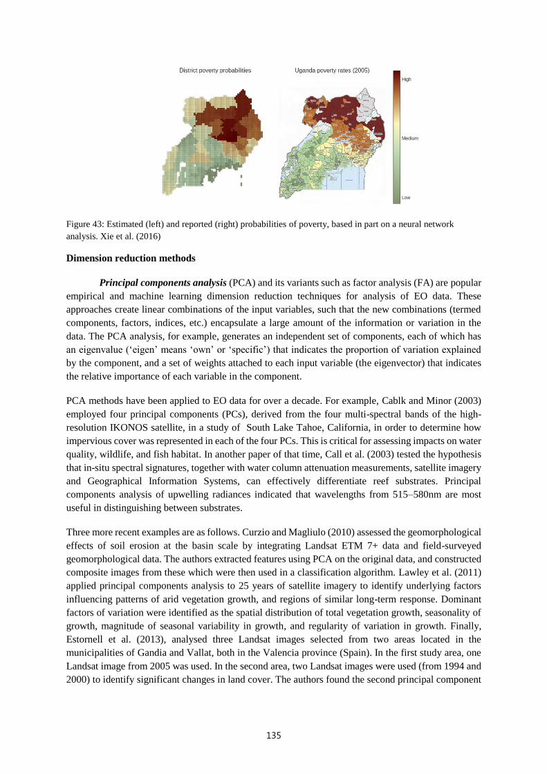
135
Figure 43: Estimated (left) and reported (right) probabilities of poverty, based in part on a neural network
analysis. Xie et al. (2016)
Dimension reduction methods
Principal components analysis (PCA) and its variants such as factor analysis (FA) are popular
empirical and machine learning dimension reduction techniques for analysis of EO data. These
approaches create linear combinations of the input variables, such that the new combinations (termed
components, factors, indices, etc.) encapsulate a large amount of the information or variation in the
data. The PCA analysis, for example, generates an independent set of components, each of which has
an eigenvalue (‘eigen’ means ‘own’ or ‘specific’) that indicates the proportion of variation explained
by the component, and a set of weights attached to each input variable (the eigenvector) that indicates
the relative importance of each variable in the component.
PCA methods have been applied to EO data for over a decade. For example, Cablk and Minor (2003)
employed four principal components (PCs), derived from the four multi-spectral bands of the high-
resolution IKONOS satellite, in a study of South Lake Tahoe, California, in order to determine how
impervious cover was represented in each of the four PCs. This is critical for assessing impacts on water
quality, wildlife, and fish habitat. In another paper of that time, Call et al. (2003) tested the hypothesis
that in-situ spectral signatures, together with water column attenuation measurements, satellite imagery
and Geographical Information Systems, can effectively differentiate reef substrates. Principal
components analysis of upwelling radiances indicated that wavelengths from 515–580nm are most
useful in distinguishing between substrates.
Three more recent examples are as follows. Curzio and Magliulo (2010) assessed the geomorphological
effects of soil erosion at the basin scale by integrating Landsat ETM 7+ data and field-surveyed
geomorphological data. The authors extracted features using PCA on the original data, and constructed
composite images from these which were then used in a classification algorithm. Lawley et al. (2011)
applied principal components analysis to 25 years of satellite imagery to identify underlying factors
influencing patterns of arid vegetation growth, and regions of similar long-term response. Dominant
factors of variation were identified as the spatial distribution of total vegetation growth, seasonality of
growth, magnitude of seasonal variability in growth, and regularity of variation in growth. Finally,
Estornell et al. (2013), analysed three Landsat images selected from two areas located in the
municipalities of Gandia and Vallat, both in the Valencia province (Spain). In the first study area, one
Landsat image from 2005 was used. In the second area, two Landsat images were used (from 1994 and
2000) to identify significant changes in land cover. The authors found the second principal component

136
of the Gandia area image allowed detection of the presence of vegetation. The same component in the
Vallat area allowed detection of a forestry area affected by forest fire.
Although PCA is a highly useful and effective method for dimension reduction in satellite image
analysis, like any dimension reduction method it does possess a shortcoming: the dominant components
(factors) do not contain all of the information in the data. Thus the common practice of choosing only
the dominant components and using these for further interpretation and analysis can sometimes lead to
inaccurate estimation of covariance matrices and may also lead to a loss of spatial information. Other
caveats for PCA are that it may not be reliable if only a small number of images are available, and it
can be quite time and resource intensive when applied to large image data. Various extensions to PCA
have been proposed to overcome some of these issues.
Independent Component Analysis (ICA) is a technique which finds so-called “independent
components” of observed data. This data is assumed to be realisations of linear mixtures of unknown
latent variables (the independent components) which in turn are assumed to be non-Gaussian and
mutually independent. ICA separates a multivariate signal into additive subcomponents.
Independent Component Analysis is related, in a certain sense, to both principal component analysis
and factor analysis. However, one of the advantages of ICA over these techniques is that it will often
work in situations where the former may fail.
A.2 Summary of methods for static data
The following table summarises some of the techniques discussed above and provides some guidance
in the selection of the most appropriate technique under certain situations. It is important to recognise
that each technique has its own merits and limitations, and that in any particular application the use of
more than one technique may provide greater insight than the use of any one in isolation.

137
Technique Parametric?
Computational
Load (training
speed)
Amount of
Parameter
Tuning
Required
Probabilities
of Class
Membership?
Spatial and
Temporal
Dependencies?
Small amount of
Training Data?
Tendency To
Overfit?
SVM No Slow Significant No No Yes No
Neural
Networks No Moderate Significant No No Maybe Yes
Decision
trees No Fast Low Yes No No Yes
Boosted
Regression
Trees
No Fast Low Yes No No Unsure
Multinomi
al Logistic
regression
Yes Slow Moderate Yes Can be modified No No, under user
control
K-nn No Fast Low No No No Yes
SSMs Yes Slow Moderate Depends Yes No Under user control
INLA-
Based Yes
Faster than
equivalent
options such as
MCMC
Moderate Depends Yes No Under user control

138
A.3 Methods for analysis of dynamic data
As described in Chapter 3, there is a variety of heuristic, statistical and machine learning methods for
analysing EO data over time.
Comparative approaches
These approaches are popular, as described in Section 3. Fulcher et al (2014) describe how the two
approaches outlined in that section can be used for classification. By creating a database of known
time series and their classifications, a new time series can be classified by comparing the distance
measures between the series in the database. The method proposed by Fulcher et al (2014) learns the
properties of a given class of time series and classifies new time series according to these learned
properties.
Figure 44: Comparing time series by their structural features
Source: Fulcher et al (2014). What’s the difference? Telling apart two sets of signals. Retrieved from: http://systems-signals.blogspot.com.au/
Cubic splines
These models are semi-parametric regression equations which fit a series of (cubic) polynomials to
the temporal data (Pollock, 2009); see, for example Reed et al. (1994) for an example of their use in
analysis of Normalised Difference Vegetation Index (NDVI) phenological parameters using satellite
imagery.
Figure 45: Modelling crop growth (left) using a cubic spline model (right)
Harmonic models
These models fit more structured sinusoidal (shaped like a sine curve) curves to the data. Here, the
model parameters are the phase and amplitude. For example, Potgieter and coauthors (2007, 2010,

139
2011) employ these models for crop estimation using EO data. The Enhanced Vegetation Index (EVI)
from 16-day MODIS satellite imagery within the cropping period (i.e. April–November) was
investigated to estimate crop area for wheat, barley, chickpea, and total winter cropped area for a case
study region in northeast Australia. The authors found significant overall capability to estimate total
winter crop area and high accuracy at pixel scale (>98% correct classification) for identifying overall
winter cropping. However, discrimination among crops was less accurate.
Figure 46: Illustration of harmonic analysis (left) and its application to MODIS imagery of time series of winter
crops in 2005 (top right) and 2006 (bottom right). Potgeiter et al. (2007, 2011, 2013)
Spectral decomposition
Just as Principal Components Analysis (PCA) and Independent Components Analysis (ICA) are forms
of dimension reduction for static data, spectral decomposition methods such as Fourier transforms can
be used as dimension reduction techniques for dynamic data. These methods extract important
information from high dimensional space to a smaller dimensional space. The analysis can be an end in
itself, or the smaller dimensional space can then be fed to another statistical or machine learning
algorithm to form an ensemble approach.
Following on from the example described above, Potgieter et al. (2007) utilise spectral decomposition
in the form of the Fast Fourier Transform on MODIS time series data, the results of which are then used
in a discriminant analysis. A similar approach (spectral decomposition of remotely sensed temporal
data being fed to a discriminant analysis supervised classification technique) was undertaken in
Potgieter et al. (2011). An alternative approach is to fit parametric curves to remotely sensed crop
growth data (the previous approaches could be categorised as non-parametric in this sense). Potgieter
et al. (2013) utilise parametric Gaussian functional curves to reduce data dimensionality, and again
classify the resultant curve parameters via discriminant analysis. It is not always clear whether the
discriminant analysis assumptions (multivariate normality, for example) are met in these cases.
HANTS (Verhoef et al 1996)
(a)
(b)
(c)
Amplitude
Phase
0 353
Day of Year (DOY)
(a)
(b)
(c)
Amplitude
Phase
(a)
(b)
(c)
(a)
(b)
(c)
Amplitude
Phase
0 353
Day of Year (DOY)
(a )
0
1000
2000
3000
4000
5000
6000
7000
1
17
33
49
65
81
97
11
3
12
9
14
5
16
1
17
7
19
3
20
9
22
5
24
1
25
7
27
3
28
9
30
5
32
1
33
7
35
3
DOY
EV
I
Actual
Reconstructed
(b )
0
1000
2000
3000
4000
5000
6000
7000
1
17
33
49
65
81
97
11
3
12
9
14
5
16
1
17
7
19
3
20
9
22
5
24
1
25
7
27
3
28
9
30
5
32
1
33
7
35
3
DOY
EV
I
Actual
Reconstructed

140
Functional data analysis (FDA)
FDA is a nonparametric method for describing and classifying curves, in which each sample point in
the time series is considered to be a function observed along an underlying continuum (e.g. time). This
provides great flexibility in describing the underlying curve.
FDA approaches have been around for over two decades. For example, a FDA method for logistic
regression was described by Escabias et al. (2005). In this paper, the authors modelled the relationship
between the risk of drought and curves of temperatures. A functional logistic regression model was also
employed to predict land use based on the temporal evolution of coarse-resolution EO remote sensing
data by Cardot et al. (2003).
A more recent paper on this topic is by Liu et al. (2012) on rotating functional factor analyses to improve
estimation of periodic temporal trends in EO data. These authors demonstrated their approach on a six-
year time series at 8-day intervals of vegetation index measurements obtained from remote sensing
images.
State space models
State space models have been recommended by the Australian Bureau of Statistics (ABS) for the
analysis of dynamic EO data. See the paper by Tam and Clark (2015) on “A Statistical Framework for
Analysing Big Data” for an exposition of the use of SSMs with reference to official statistics.
State space models are a very common form of spatio-temporal model that can provide a natural setting
for analysing time series of EO data, particularly if the process to be modelled can be viewed as one
that is spatially evolving through time. Depending on the nature of the data (geostatistical or
lattice/areal), various spatial, temporal, and spatio-temporal dependency structures can be incorporated
into the model. Cressie and Wikle (2011) devote an entire chapter (Chapter 7) to the various
permutations of spatial and temporal dependency models that can be incorporated into what they denote
as Dynamic Spatio‐Temporal Models (DSTMs), and a further chapter (Chapter 8) to methods of
inference for these models.
By far the most common approach to modelling spatio-temporal data is to assume a spatial process
evolving through time (e.g. Chen et al. (2006), Waller et al. (1997), Lagazio et al. (2001), Knorr-Held
and Besag (1998), Mugglin et al. (2002), Jin et al. (2005), Jin et al. (2005), Norton and Niu (2009),
Allcroft and Glaseby (2003), Zhu et al. (2005), Zhu et al. (2008), Zheng and Zhu (2008), Daniels et al.
(2006), Ugarte et al. (2010)). As noted in Cressie and Wikle (2011), this approach is conceptually
reasonable in many applications, and enables the spatio-temporal process to fit within the remit of a
dynamic spatial modelling approach, or the state space modelling framework. This approach was
investigated by the Australian Bureau of Statistics as a pilot project.
A linear Gaussian state space model takes the general form
𝑌𝑡 = 𝐻𝑡𝑋𝑡 + 𝑣𝑡 , 𝑣𝑡 ∼ 𝑁𝑚𝑡(0, 𝑅𝑡)
𝑋𝑡 = 𝑀𝑡𝑋𝑡−1 + 𝑤𝑡 , 𝑤𝑡 ∼ 𝑁𝑛(0, 𝑄𝑡) ,
where, for time 𝑡, 𝑡 = 1, ⋯ , 𝑇, 𝑌𝑡 denotes the 𝑚𝑡‐dimensional data vector, 𝑋𝑡 denotes the n‐dimensional
unobserved “state” vector, 𝑣𝑡 is the serially independent observation error, and 𝑤𝑡 is the serially
independent innovation error (Shumway and Stoffer, 2011). It is generally assumed that 𝑣𝑡 and 𝑤𝑡 are
mutually independent. It is also generally assumed that the observation matrix 𝐻𝑡, the state transition

141
matrix 𝑀𝑡 (also known as the evolution or propagator matrix), and the two covariance matrices 𝑅𝑡 and
𝑄𝑡, are known, although this can be relaxed.
Typically the main mechanism for incorporating spatio-temporal dependencies is through the
covariance matrices 𝑅𝑡 and 𝑄𝑡. It is common, for example, to view the states 𝑋𝑡 as being driven not
only by temporal processes but also by spatial ones, thus some form of spatial structure is placed on 𝑄𝑡.
This may take the form of one of the common covariance function structures for geostatistical data or
perhaps a sparse, neighbour-based covariance matrix induced by assuming a Markov random field in
lattice data. Spatial, temporal, or spatio-temporal structures can also be assumed on the measurement
structure.
Extensions to these models include non-Gaussian state-space models, non-linear observation equation
models, agent-based approaches, generalised additive mixed effects models and multivariate response
models. Another important area of research in this context is dimension reduction via spectral
decompositions. Such dimension reduction can substantially reduce computational load when fitting
these dynamic models to data.
State space models have been employed for crop estimation and prediction for over 15 years. For
example, Wendroth et al. (2003) used this approach to predict yield of barley across a landscape. More
recently, Schneibel et al. (2017) applied the method to annual Landsat time series data with the aim of
detecting dry forest degradation processes in South-Central Angola.
An example of using a Hidden Markov Model to analyse EO data is given by Yuan et al. (2015) in the
context of detecting urban encroachment onto farmland in China. Two sources of data were used in this
study:
• MODIS data 2001-2010 (large-scale coverage, high temporal resolution [16 day], open)
downloaded from the Level 1 and Atmosphere Archive and Distribution System (LAADS)
website; this provided four spectral reflectance bands for vegetation and land surface, i.e., band
1 (red: 620–670 nm), band 2 (NIR: 841–875 nm), band 3 (blue: 459–479 nm), band 7 (MIR:
2105–2155 nm)
• ESA Global Land Cover (GlobCover) map for 2009, for model training: farmland, built-up
classes.
As a pre-processing step, Functional Analysis (via a Fourier model, see above) was used to create high
quality time series of band reflectances. A k-means analysis was also employed to cluster land use,
using training data. A sliding window was then used to smooth estimates and a Hidden Markov Model
was employed to identify change in classes. The authors obtained 96% correct change detection and
0.04% false alarm.

142
Figure 47: (Top) Functional analysis employed to interpolate EO data time series. (Middle) K-means clustering
employed to classify farmland. (Bottom) Hidden Markov model to identify urban encroachment. Yuan et al.
(2015)
A.4 Choice between methods
Comparisons between various empirical methods and machine learning approaches have been made for
over a decade. Advantages and disadvantages of the different methods depend on the nature of the
problem. Some examples of these comparisons are as follows:
• A comparison was made by Hogland et al. (2013) between the ML technique and multinomial
(a.k.a. polytomous) logistic regression for the analysis of remotely sensed data. Their
conclusion was that the logistic regression methods were less restrictive, more flexible and
easier to interpret. The authors also referenced papers that show these approaches perform at
least as well as other machine learning techniques; see below.
• De Melo et al. (2003) compared ML with Gaussian mixture models for supervised
classification of remote sensing multispectral images, with a general preference for Gaussian
mixture models.
• Shao and Lunetta (2012) compared support vector machines (SVMs) to neural networks and
CART (classification and regression trees) on limited training data for Land cover
classification using MODIS time series data.
• Otukei and Blaschke (2010) considered land cover change assessment using decision trees,
SVMs (with a radial basis kernel function), and the maximum likelihood classifier and
concluded that decision trees performed best.
• Szuster et al. (2011) compared maximum likelihood classification and ANNs to SVMs for land
use and land cover classification in tropical coastal zones.
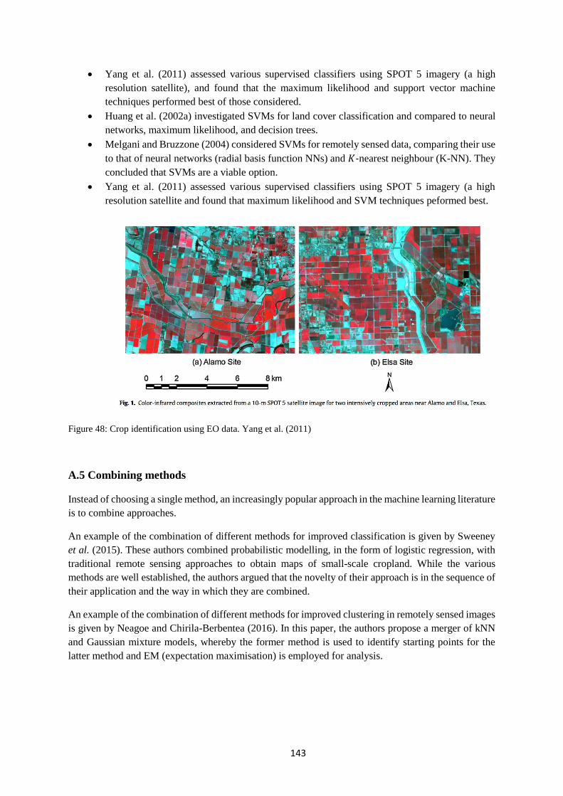
143
• Yang et al. (2011) assessed various supervised classifiers using SPOT 5 imagery (a high
resolution satellite), and found that the maximum likelihood and support vector machine
techniques performed best of those considered.
• Huang et al. (2002a) investigated SVMs for land cover classification and compared to neural
networks, maximum likelihood, and decision trees.
• Melgani and Bruzzone (2004) considered SVMs for remotely sensed data, comparing their use
to that of neural networks (radial basis function NNs) and 𝐾‐nearest neighbour (K-NN). They
concluded that SVMs are a viable option.
• Yang et al. (2011) assessed various supervised classifiers using SPOT 5 imagery (a high
resolution satellite and found that maximum likelihood and SVM techniques peformed best.
Figure 48: Crop identification using EO data. Yang et al. (2011)
A.5 Combining methods
Instead of choosing a single method, an increasingly popular approach in the machine learning literature
is to combine approaches.
An example of the combination of different methods for improved classification is given by Sweeney
et al. (2015). These authors combined probabilistic modelling, in the form of logistic regression, with
traditional remote sensing approaches to obtain maps of small-scale cropland. While the various
methods are well established, the authors argued that the novelty of their approach is in the sequence of
their application and the way in which they are combined.
An example of the combination of different methods for improved clustering in remotely sensed images
is given by Neagoe and Chirila-Berbentea (2016). In this paper, the authors propose a merger of kNN
and Gaussian mixture models, whereby the former method is used to identify starting points for the
latter method and EM (expectation maximisation) is employed for analysis.

144
References
ABARES, (2016). Agricultural Commodity Statistics 2016. Australian Bureau of Agricultural and
Resource Economics and Sciences, Canberra. Retrieved from
www.agriculture.gov.au/abares/publications/display?url=http://143.188.17.20/anrdl/DAFFService/dis
play.php%3Ffid%3Dpb_agcstd9abcc0022016_Sn9Dg.xml
Adams, J. B., Sabol, D. E., Kapos, V., Almeida Filho, R., Roberts, D. A., Smith, M. O. and
Gillespie, A. R. (1995). Classification of multispectral images based on fractions of endmembers:
Application to land-cover change in the Brazilian Amazon. Remote sensing of Environment, 52(2),
137–154.
Allcroft, D. J. and Glaseby, C. A. (2003). A latent Gaussian Markov random field model for spatio-
temporal rainfall disaggregation. Journal of the Royal Statistical Society. Series C: Applied
Statistics, 52(4), 487–498.
Al-Obeidat, F., Al-Taani, A. T., Belacel, N., Feltrin, L. and Banerjee, N. (2015). A Fuzzy Decision
Tree for Processing Satellite Images and Landsat Data. Procedia Computer Science, 52, 1192–1197.
Anderson, K., Ryan, B., Sonntag, W., Argyro, K., Friedl, L. (2017) Earth observation in service of the
2030 Agenda for Sustainable Development, Geo-spatial Information Science, 20:2, 77-96.
Aplin, P. and Atkinson, P. M. (2001). Sub-pixel land cover mapping for per-field classification.
International Journal of Remote Sensing, 22(14), 2853–2858.
Aplin, P., Atkinson, P. M., Curran, P. J. and Others (1999). Per-field classification of land use using
the forthcoming very fine spatial resolution satellite sensors: problems and potential solutions.
Advances in remote sensing and GIS analysis, pp. 219–239.
Atkinson, P. M. and Tatnall, A. R. L. (1997). Introduction neural networks in remote sensing.
International Journal of remote sensing, 18(4), 699–709.
Augustin, N. H., Musio, M., von Wilpert, K., Kublin, E., Wood, S. N. and Schumacher, (2009).
Modelling spatio temporal forest health monitoring data. Journal of the American Statistical
Association,104 (487), 899-911.
Baıllo, A., Cuesta-Albertos, J. A. and Cuevas, A. (2011a). Supervised Classification for a Family of
Gaussian Functional Models. Scandinavian Journal of Statistics, 38, 480– 498.
Baıllo, A., Cuevas, A. and Fraiman, R. (2011b). Classification Methods for Functional Data. In The
Oxford Handbook of Functional Data Analysis. (Eds F. Ferraty and Y. Romain), pp. 259–297. Oxford:
Oxford University Press, UK.
Banerjee, S., Carlin, B. P. and Gelfand, A. E. (2014). Hierarchical modeling and analysis for spatial
data. Crc Press, second edition.
Banerjee, S., Gelfand, A. E., Finley, A. O. and Sang, H. (2008). Gaussian Predictive Process Models
for Large Spatial Data Sets. Journal of the Royal Statistical Society. Series B (Statistical Methodology),
70(4), 825–848.

145
Bastin, L. (1997). Comparison of fuzzy c-means classification, linear mixture modelling and MLC
probabilities as tools for unmixing coarse pixels. International Journal of Remote Sensing, 18(17),
3629–3648.
Bateson, C., Asner, G. P., Wessman, C. and Others (2000). Endmember bundles: A new approach to
incorporating endmember variability into spectral mixture analysis. Geo- science and Remote
Sensing, IEEE Transactions on, 38(2), 1083–1094.
Bavaghar, P. (2015) Deforestation modelling using logistic regression and GIS. Journal of Forest
Science 61, 193-199.
Bédard, F. and Reichert, G. (2013). Integrated Crop Yield and Production Forecasting using Remote
Sensing and Agri-Climatic data. Analytical Projects Initiatives final report. Remote Sensing and
Geospatial Analysis, Agriculture Division, Statistics Canada
Benediktsson, J. A. and Swain, P. H. (1992). Consensus theoretic classification methods. IEEE Trans.
Syst., Man, Cybern., vol. 22, 688–704.
Benediktsson, J. A., Sveinsson, J. R. and Swain, P. H. (1997). Hybrid consensus theoretic
classification. Geoscience and Remote Sensing, IEEE Transactions on, 35(4), 833–843.
Benz, U. C., Hofmann, P., Willhauck, G., Lingenfelder, I. and Heynen, M. (2004). Multi- resolution,
object-oriented fuzzy analysis of remote sensing data for GIS-ready information. ISPRS Journal of
photogrammetry and remote sensing, 58(3), 239–258.
Berliner, L. M., Wikle, C. K. and Cressie, N. (2000). Long-lead prediction of Pacific SSTs via Bayesian
dynamic modeling. Journal of Climate, 13(22), 3953–3968.
Berliner, L. M., Wikle, C. K. and Milliff, R. F. (1999). Multiresolution wavelet analyses in hierarchical
Bayesian turbulence models. In Bayesian inference in wavelet-based models (Eds P. Mueller and B.
Vidakovic), Chapter 21, pp. 341–359. New York: Springer.
Bernardinelli, L., Clayton, D., Pascutto, C., Montomoli, C., Ghislandi, M. and Songini, M. (1995).
Bayesian analysis of space–time variation in disease risk. Statistics in medicine, 14(21-22), 2433–2443.
Besag, J. (1974). Spatial interaction and the statistical analysis of lattice systems. Journal of the Royal
Statistical Society. Series B (Methodological), 36(2), 192–236.
Bigdeli, B., Samadzadegan, F. and Reinartz, P. (2015). Fusion of hyperspectral and LIDAR data using
decision template-based fuzzy multiple classifier system. International Journal of Applied Earth
Observation and Geoinformation, 38, 309–320.
Billheimer, D., Cardoso, T., Freeman, E., Guttorp, P., Ko, H. W. and Silkey, M. (1997). Natural
variability of benthic species composition in the Delaware Bay. Environmental and Ecological
Statistics, 4(2), 95–115.
Blangiardo, M., Cameletti, M., Baio, G. and Rue, H. H. (2013). Spatial and spatio– temporal
models with R--INLA. Spatial and Spatio–temporal Epidemiology, 7, 39–55.
Blanzieri, E. and Melgani, F. (2008). Nearest neighbor classification of remote sensing images with
the maximal margin principle. Geoscience and Remote Sensing, IEEE Transactions on, 46(6),
1804–1811.

146
Bolin, D. and Lindgren, F. (2013). A comparison between Markov approximations and other
methods for large spatial data sets. Computational Statistics & Data Analysis, 61, 7–21.
Bradley, J. R., Wikle, C. K. and Holan, S. H. (2016) Bayesian Spatial Change of Support for Count-
Valued Survey Data with Application to the American Community Survey. Journal of the American
Statistical Association, 0(ja), 1–43.
Breiman, L. (1996). Bagging Predictors. Machine Learning, 24(2), 123–140.
Breiman, L. (2001) Statistical modeling: the two cultures. Statistical Science 16(9), 199-231.
Breiman, L., Friedman, J., Stone, C. J. and Olshen, R. A. (1984). Classification and Regression
Trees. CRC press.
Briem, G. J., Benediktsson, J. A. and Sveinsson, J. R. (2002). Multiple classifiers applied to
multisource remote sensing data. Geoscience and Remote Sensing, IEEE Transactions on, 40(10),
2291–2299.
Brynjarsdottir, J. and Berliner, M. (2014). Dimension–Reduced Modelling of Spatio– Temporal
Processes. Journal of the American Statistical Association, 109(508), 1647– 1659.
Cablk, M.E. and Minor, T.B. (2003). Detecting and discriminating impervious cover with high-
resolution IKONOS data using principal component analysis and morphological operators.
International Journal of Remote Sensing, 24: 4627–4645.
C alıs, N. and Erol, H. (2012). A new per-field classification method using mixture discriminant
analysis. Journal of Applied Statistics, 39(10), 2129–2140.
Calder, C. A. (2007). Dynamic factor process convolution models for multivariate space- time data
with application to air quality assessment. Environmental and Ecological Statistics, 14(3), 229–247.
Call , K.A., Hardy, J.T., and Wallin, D. O. (2003). Coral reef habitat discrimination using multivariate
spectral analysis and satellite remote sensing. International Journal of Remote Sensing, 24: 2627–
2639.
Cao, Q., Guo, Z. and Yang, Y. (2015). An improved back propagation neural network approach to
the remote sensing land use and land cover classification. Computer Science and Applications:
Proceedings of the 2014 Asia-Pacific Conference on Computer Science and Applications (CSAC 2014),
Shanghai, China, 27-28 December 2014, 369. CRC Press.
Cardot H, Faivre R, Goulard M (2003) Functional approaches for predicting land use with the
temporal evolution of coarse resolution remote sensing data. Journal of Applied Statistics 30: 1185-
1199.
Carlin, B. P., Polson, N. G. and Stoffer, D. S. (1992). A Monte Carlo approach to non-normal and
nonlinear state-space modelling. Journal of the American Statistical Association, 87(418), 493–500.
Carr, J. R. (1999). Classification of digital image texture using variograms. Advances in remote
sensing and GIS analysis, pp. 135–146.
Cavalli, R.M., Licciardi, G.A., and Chanussot, J. (2013). Detection of Anomalies Produced by Buried
Archaeological Structures Using Nonlinear Principal Component Analysis Applied to Airborne

147
Hyperspectral Image. IEEE Journal of Selected Topics in Applied Earth Observations and Remote
Sensing, 6: 659 – 669.
Chasmer, L., Hopkinson, C., Veness, T., Quinton, W. and Baltzer, J. (2014). A decision- tree
classification for low-lying complex land cover types within the zone of discontinuous permafrost.
Remote Sensing of Environment, 143, 73–84.
Chen, K. S., Tzeng, Y. C., Chen, C. F. and Kao, W. L. (1995). Land-cover classification of
multispectral imagery using a dynamic learning neural network. Photogrammetric Engineering and
Remote Sensing, 61(4), 403–408.
Chen, L., Fuentes, M. and Davis, J. M. (2006). Spatial-temporal statistical modelling and prediction
of environmental processes. In Hierarchical Modelling for the Environmental Sciences: Statistical
methods and applications (Eds J. S. Clark and A. E. Gelfand), chapter 7, pp. 121–144. New York:
Oxford University Press.
Chiang, S.-S., Chang, C.-I. and Ginsberg, I. W. (2000). Unsupervised hyperspectral image analysis
using independent component analysis. Geoscience and Remote Sensing Symposium Proceedings.
IGARSS 2000. IEEE 2000 International, volume 7, pp. 3136–3138.
Chipanshi, A., Zhang, Y., Kouadio, L., Newlands, N., Davidson, A., Hill, H., Warren, R., Qian, B.,
Daneshfar, B., Bedard, F. and Reichert, G. (2015). Evaluation of the Integrated Canadian Crop Yield
Forecaster (ICCYF) Model for In-season Prediction of Crop Yield across the Canadian Agricultural
Landscape. Agricultural and Forest Meteorology, 206:137-150. DOI:
http://dx.doi.org/10.1016/j.agrformet.2015.03.007
Clark, J. S. and Gelfand, A. E. (2006). Hierarchical Modelling for the Environmental Sciences:
Statistical methods and applications. New York: Oxford University Press, UK.
Clayton, D. G. (1996). Generalized Linear Mixed Models. In Markov Chain Monte Carlo in Practice
(Eds W. Gilks, S. Richardson and D. Spiegelhalter), 275–301. Chapman & Hall.
Clayton, D. G. and Bernardinelli, L. (1992). Bayesian methods for mapping disease risk. In
Geographical and Environmental Epidemiology: Methods for Small–Area Studies (Eds P. Elliot, J.
Cuzick, D. English and R. Stern), 205–220. UK: Oxford University Press.
Cliff, A. D. and Ord, J. K. (1981). Spatial processes: models and applications. London, UK: Pion.
Clinton, N., Yu, L. and Gong, P. (2015). Geographic stacking: Decision fusion to increase global land
cover map accuracy. ISPRS Journal of Photogrammetry and Remote Sensing, 103, 57–65.
Collins, M. J., Dymond, C. and Johnson, E. A. (2004). Mapping subalpine forest types using networks
of nearest neighbour classifiers. International Journal of Remote Sensing, 25(9), 1701–1721.
Cowles, M. K. (2003). Efficient model-fitting and model-comparison for high-dimensional Bayesian
geostatistical models. Journal of Statistical Planning and Inference, 112(1-2), 221–239.
Crammer, K. and Singer, Y. (2002). On the algorithmic implementation of multiclass kernel-based
vector machines. The Journal of Machine Learning Research, 2, 265– 292.
Cressie, N. A. C. (1993). Statistics for Spatial Data Revised Edition. Wiley Series in probablility
and mathematical statistics. New York: John Wiley & Sons, Inc.

148
Cressie, N. and Huang, H.-C. (1999). Classes of nonseparable, spatio-temporal stationary covariance
functions. Journal of the American Statistical Association, 94(448), 1330– 1339.
Cressie, N. and Verzelen, N. (2008). Conditional-mean least-squares fitting of Gaussian Markov
random fields to Gaussian fields. Computational Statistics and Data Analysis, 52(5), 2794–2807.
Cressie, N. and Wikle, C. K. (2011). Statistics for Spatio–Temporal Data. Wiley.
Cressie, N., Shi, T. and Kang, E. L. (2010a). Fixed Rank Filtering for Spatio-Temporal Data.
Journal of Computational and Graphical Statistics, 19(3), 724–745.
Cressie, N., Shi, T. and Kang, E. L. (2010b). Fixed rank filtering for spatio–temporal data.
Cuevas, A. (2014). Journal of Statistical Planning and Inference A partial overview of the theory of
statistics with functional data. Journal of Statistical Planning and Inference, 147, 1–23.
Curzio, S.L. and Magliulo, P. (2010). Soil erosion assessment using geomorphological remote sensing
techniques: an example from southern Italy. Earth Surface Processes and Landforms 35: 262–271.
Daniels, M. J., Zhou, Z. and Zou, H. (2006). Conditionally Specified Space-Time Models for
Multivariate Processes. Journal of Computational and Graphical Statistics, 15(1), 157–177.
De Fries, R. S., Hansen, M., Townshend, J. R. G. and Sohlberg, R. (1998). Global land cover
classifications at 8 km spatial resolution: the use of training data derived from Landsat imagery in
decision tree classifiers. International Journal of Remote Sensing, 19(16), 3141–3168.
De Melo, A.C.O, de Moraes, R.M., dos Santos Machado, L. (2003) Gaussian mixture models for
supervised classification of remote sensing multispectral images. In Progress in Pattern Recognition,
Speech and Image Analysis, Volume 2905 of the series Lecture Notes in Computer Science, pp. 440-
447.
De Wit, A. J. W. and Clevers, J. (2004). Efficiency and accuracy of per-field classification for
operational crop mapping. International journal of remote sensing, 25(20), 4091– 4112.
Dekker, A., Peters, S., Vos, R., Rijkeboer, M. (2013) Remote sensing for inland water quality
detection and monitoring: state-of-the-art application in Friesland waters. In van Dijk, A., Bos, G.
(Eds) GIS and Remote Sensing Techniques in Land and Water management. CRC Press. Chapter 3.
Delaigle, A. and Hall, P. (2012a). Achieving near perfect classification for functional data. Journal of
the Royal Statistical Society. Series B: Statistical Methodology, 74(2), 267– 286.
Delaigle, A. and Hall, P. (2012b). Methodology and theory for partial least squares applied to functional
data. Annals of Statistics, 40(1), 322–352.
Delaigle, A., Hall, P. and Bathia, N. (2012). Componentwise classification and clustering of functional
data. Biometrika, 99(2), 299–313.
Delsol, L., Ferraty, F. and Martinez-Calvo, A. (2011). Functional Data Analysis: An
Interdisciplinary Statistical Topic. In Statistical Learning and Data Science. (Eds.

149
Dennison, P. E. and Roberts, D. A. (2003). Endmember selection for multiple endmember spectral
mixture analysis using endmember average RMSE. Remote Sensing of Environment, 87(2), 123–
135.
Diggle, P. J. and Ribeiro, P. J. J. (2007). Model–Based Geostatistics. New York: Springer.
Doucet, A., de Freitas, N. and Gordon, N. (eds) (2001). Sequential Monte Carlo methods in practice.
New York: Springer Science & Business Media.
Du, P., Xia, J., Zhang, W., Tan, K., Liu, Y. and Liu, S. (2012). Multiple classifier system for remote
sensing image classification: A review. Sensors, 12(4), 4764–4792.
Elith, J., Leathwick, J.R., Hastie, T. (2008) A working guide to boosted regression trees. Journal of
Animal Ecology 77, 802-813.
Erbek, F. S., O zkan, C. and Taberner, M. (2004). Comparison of maximum likelihood
classification method with supervised artificial neural network algorithms for land use activities.
International Journal of Remote Sensing, 25(9), 1733–1748.
Erol, H. and Akdeniz, F. (2005). A per-field classification method based on mixture distribution
models and an application to Landsat Thematic Mapper data. International Journal of Remote
Sensing, 26(6), 1229–1244. Evensen, G. (2009) Data assimilation: the ensemble Kalman filter. New
York: Springer Science & Business Media, second edition.
Escabias M., Aguilera, A.M., Valderrama, M.J. (2005). Modelling environmental data by functional
principal component logistic regression. Environmetrics 16: 95-107.
Esch, T., Taubenbock, H., Roth, A., Heldens, W., Felbier, A., Thiel, M., Schmidt, M., Muller, A., Dech,
S. (2012). TanDEM-X mission – new perspectives for the inventory and monitoring of global settlement
patterns. Journal of Applied Remote Sensing 6(1), 061702-1-061702-21.
Estornell, J., Marti-Gavila, J.M. , Sebastia, M. T. and Mengual, J. (2013). Principal component
analysis applied to remote sensing. Modelling in Science Education and Learning, 6(2): 83–89.
European Commission (2016). MARS bulletins May 2016. Retrieved from
https://ec.europa.eu/jrc/en/publication/eur-scientific-and-technical-research-reports/jrc-mars-bulletin-
crop-monitoring-europe-may-2016-fairly-good-outlook-despite-unsettled
Fan, J., Han, F. and Liu, H. (2014). Challenges of Big Data analysis. National Science Review (June
2014) 1 (2): 293-314. Retrieved from http://nsr.oxfordjournals.org/content/1/2/293.full.
Febrero-Bande, M. and de la Fuente, M. O. (2012). Statistical Computing in Functional Data
Analysis: The R Package fda.usc. Journal of Statistical Software, 51(4), 1–28.
Fernandez-Prieto, D. (2002). An iterative approach to partially supervised classification problems.
International Journal of Remote Sensing, 23(18), 3887–3892.
Ferraty, F. and Romain, Y. (eds) (2011). The Oxford Handbook of Functional Data Analysis. Oxford:
Oxford University Press, UK.

150
Ferreira, M. A. R., Holan, S. H. and Bertolde, A. I. (2011). Dynamic multiscale spatiotemporal models
for Gaussian areal data. Journal of the Royal Statistical Society. Series B: Statistical Methodology,
73(5), 663–688.
Finkenstadt, B., Held, L. and Isham, V. (eds) (2007). Statistical methods for spatio- temporal
systems. Boca Raton, FL: CRC Press.
Fix, E. and Hodges Jr, J. L. (1951). Discriminatory analysis-nonparametric discrimination: consistency
properties. Technical report, DTIC Document.
Food and Agriculture Organisation (FAO) (2016). FAO Cereal Supply and Demand Brief. Retrieved
from http://www.fao.org/worldfoodsituation/csdb/en/.
Foody, G. M. (1996a). Approaches for the production and evaluation of fuzzy land cover
classifications from remotely-sensed data. International Journal of Remote Sensing, 17(7), 1317–
1340.
Foody, G. M. (1996b). Fuzzy modelling of vegetation from remotely sensed imagery. Ecological
modelling, 85(1), 3–12.
Foody, G. M. (1997). Fully fuzzy supervised classification of land cover from remotely sensed
imagery with an artificial neural network. Neural Computing & Applications, 5(4), 238–247.
Foody, G. M. (1999). Image classification with a neural network: from completely-crisp to fully-
fuzzy situations. Advances in remote sensing and GIS analysis, pp. 17–37.
Foody, G. M. and Arora, M. K. (1997). An evaluation of some factors affecting the accuracy of
classification by an artificial neural network. International Journal of Remote Sensing, 18(4), 799–
810.
Foody, G. M., Lucas, R. M., Curran, P. J. and Honzak, M. (1997). Non-linear mixture modelling without
end-members using an artificial neural network. International Journal of Remote Sensing, 18(4),
937–953.
Foody, G. M., McCulloch, M. B. and Yates, W. B. (1995). Classification of remotely sensed data
by an artificial neural network: issues related to training data characteristics. Photogrammetric
Engineering and Remote Sensing, 61(4), 391–401.
Franco-Lopez, H., Ek, A. R. and Bauer, M. E. (2001). Estimation and mapping of forest stand
density, volume, and cover type using the k-nearest neighbors method. Remote sensing of
environment, 77(3), 251–274.
Freund, Y., Schapire, R. E. and Others (1996). Experiments with a new boosting algorithm. In ICML,
volume 96, pp. 148–156.
Friedl, M. A. and Brodley, C. E. (1997). Decision tree classification of land cover from remotely
sensed data. Remote sensing of environment, 61(3), 399–409.
Friedman, J., Hastie, T. and Tibshirani, R. (2010) Regularisation Paths for Generalized Linear
Models via Coordinate Descent. Journal of Statistical Software, 33(1), 1–22.

151
Friedman, J., Hastie, T., Tibshirani, R. and Others (2000). Additive logistic regression: a statistical
view of boosting (with discussion and a rejoinder by the authors). The annals of statistics, 28(2), 337–
407.
Fruhwirth-Schnatter, S. (2006). Finite Mixture and Markov Switching Models. New York: Springer.
Fulcher, B.D., Little, M.A., Jones, N.S. (2013). Highly comparative time-series analysis: the empirical
structure of time series and their methods. Journal of the Royal Society
https://doi.org/10.1098/rsif.2013.0048
Fuentes, M., Chen, L. and Davis, J. M. (2008). A class of nonseparable and nonstationary spatial
temporal covariance functions. Environmetrics, 19, 487–507.
Gallego, J.C.M., Michaelsen, J., Bossyns, B., Fritz, S. (2008) Best practices for crop area estimation
with Remote Sensing. GEOSS Community of Practice Ag 0703a. JRC Scientific and Technical
Reports. Retrieved from
https://www.earthobservations.org/documents/cop/ag_gams/GEOSS%20best%20practices%20area%
20estimation%20final.pdf
Gao, F., Masek, J., Schwaller, M., and Hall, F. (2006). On the blending of the Landsat and MODIS
surface reflectance: predict daily Landsat surface reflectance. Remote Sensing, 44(8), 2207-2218
Gao, F., Anderson, M.C., Zhang, X., Yang, Z., Alfieri, J.G., Kustas, W.P., Mueller, R., Johnson,
D.M., and J.H. Prueger. (2017). Toward mapping crop progress at field scales using Landsat and
MODIS imagery. Remote Sens. Environ., 188, 9–25.
Geib, C., Taubenbock, H. (2013) Remote sensing contributing to assess earthquake risk: from a
literature review towards a roadmap. Natural Hazards 68 (1), 7-48.
Gelfand, A. E. and Vounatsou, P. (2003). Proper multivariate conditional autoregressive models for
spatial data analysis. Biostatistics, 4(1), 11–25.
Gelfand, A. E., Diggle, P. J., Fuentes, M. and Guttorp, P. (eds) (2010). Handbook of Spatial Statistics.
Boca Raton, FL: Chapman & Hall.
Gelfand, A. E., Schmidt, A. M., Banerjee, S. and Sirmans, C. F. (2004). Nonstationary multivariate
process modeling through spatially varying coregionalization. Test, 13(2), 263–312.
Geneletti, D. and Gorte, B. G. H. (2003). A method for object-oriented land cover classification
combining Landsat TM data and aerial photographs. International Journal of Remote Sensing, 24(6),
1273–1286.
Gettler-Summa, M., Bottou, L., Goldfarb, B., Murtagh, F., Pardoux, C., and Touati, M. (2011).
Statistical Learning and Data Science p. 189–195. Boca Raton, FL: Chapman & Hall.
Ghosh, A., Mishra, N. S. and Ghosh, S. (2011). Fuzzy clustering algorithms for unsupervised
change detection in remote sensing images. Information Sciences, 181(4), 699–715.
Ghosh, A., Subudhi, B. N. and Bruzzone, L. (2013). Integration of Gibbs Markov random field and
Hopfield-type neural networks for unsupervised change detection in remotely sensed multi-temporal
images. Image Processing, IEEE Transactions on, 22(8), 3087– 3096.

152
Global Strategy 2017. Handbook on Remote Sensing for Agricultural statistics. Rome,
www.gsars.org, 250pp.
Gneiting, T. (2002). Nonseparable , Stationary Covariance Functions for Space-Time Data. Journal of
the American Statistical Association, 97(458), 590–600.
Goldfarb, B., Murtagh, F., Pardoux, C., and Touati, M., pp. 197–203. Boca Raton, FL: Chapman &
Hall.
Gonzalez - Manteiga, W. and Vieu, P. (2011). Methodological Richness of Functional Data Analysis. In
Statistical Learning and Data Science.
Gordon, N., Salmond, D. and Smith, A. (1993). Novel approach to nonlinear/non-Gaussian Bayesian
state estimation. IEE Proceedings F Radar and Signal Processing, 140(2), 107–113.
Grenzdörffer, G. (2001). Requirements and possibilities of remote sensing for precision agriculture -
current status and future developments. In: Grenier, G., and Blackmoore S. [ed.] (2001). Proceedings
of the Third European Conference on Precision Agriculture, Montpellier June 18th-21st, 1, 211 – 216.
Guerschman, J. P. , Donohue, R. J., Van Niel T. G., Renzullo L. J., Dekker A. G. , Malthus T. J.,
McVicar T. R. and Van Dijk, A. I. J. M. (2016). Earth observation for water resources management
Part II in Earth observation for water resources management: current use and future opportunities for
the water sector, (2016) Eds. García, L., Rodríguez, D., Wijnen, M. and Pakulski, I., World Bank,
Washington, US. ISBN: 978-1-4648-0475-5; e-ISBN: 978-1-4648-0476-2 ;
http://dx.doi.org/10.1596/978-1-4648-0475-5., PDF:
https://openknowledge.worldbank.org/bitstream/handle/10986/22952/9781464804755.pdf
Guha, S., Hafen, R., Rounds, J., Xia, J., Li, J., Xi, B. and Cleveland, W. S. (2012). Large complex
data: divide and recombine (D & R ) with RHIPE. Stat, 1, 53–67.
Haapanen, R., Ek, A. R., Bauer, M. E. and Finley, A. O. (2004). Delineation of forest/nonforest
land use classes using nearest neighbor methods. Remote Sensing of Environment, 89(3), 265–271.
Han, M. and Liu, B. (2015). Ensemble of extreme learning machine for remote sensing image
classification. Neurocomputing, 149, 65–70.
Hansen, M. C., DeFries, R. S., Townshend, J. R. G. and Sohlberg, R. (2000). Global land cover
classification at 1 km spatial resolution using a classification tree approach. International journal of
remote sensing, 21(6-7), 1331–1364.
Hansen, M., Dubayah, R. and DeFries, R. (1996). Classification trees: an alternative to traditional
land cover classifiers. International journal of remote sensing, 17(5), 1075– 1081.
Hardin, P. J. (1994). Parametric and nearest-neighbor methods for hybrid classification: a comparison
of pixel assignment accuracy. Photogrammetric Engineering and Remote Sensing, 60(12), 1439–
1448.
Hardin, P. J. and Thomson, C. N. (1992). Fast nearest neighbor classification methods for
multispectral imagery. The Professional Geographer, 44(2), 191–202.
Hastie, T., Tibshirani, R. and Friedman, J. (2009). The Elements of Statistical Learning Data
Mining, Inference and Prediction. New York: Springer, second edition.
153
Hentze, K., Thonfeld, F. and Menz, G. (2016). Evaluating Crop Area Mapping from MODIS Time-
Series as an Assessment Tool for Zimbabwe’s “Fast Track Land Reform Programme”. PloS
one, 11(6).
Hogland, J., Billor, N., Anderson, N. (2013) Comparison of standard maximum likelihood
classification and polytomous logistic regression used in remote sensing. European Journal of Remote
Sensing 46, 623-640.
Hooten, M. B. and Wikle, C. K. (2008). A hierarchical Bayesian non-linear spatio- temporal
model for the spread of invasive species with application to the Eurasian Collared-Dove.
Environmental and Ecological Statistics, 15(1), 59–70.
Hooten, M. B. and Wikle, C. K. (2010). Statistical Agent-Based Models for Discrete Spatio-
Temporal Systems. Journal of the American Statistical Association, 105(October 2014), 236–248.
Hooten, M. B., Wikle, C. K., Dorazio, R. M. and Royle, J. A. (2007). Hierarchical spatio-temporal
matrix models for characterizing invasions. Biometrics, 63(2), 558–567.
Hoque, Phinn, S. et al. (2016) Assessing tropical cyclone impacts using object-based moderate spatial
resolution image analysis: a case study in Bangladesh. International Journal of Remote
Sensing, 37 22: 5320-5343.
Hoque, Phinn, S. et al. (2017): Modelling tropical cyclone risks for present and future climate change
scenarios using geospatial techniques. International Journal of Digital Earth, 1-18.
Horvath, L. and Kokoszka, P. (2012). Inference for Functional Data with Applications. New York:
Springer.
Huang, C., Davis, L. S. and Townshend, J. R. G. (2002). An assessment of support vector machines for
land cover classification. International Journal of Remote Sensing, 23(4), 725–749.
Huang, G., Huang, G. B., Song, S. and You, K. (2015). Trends in extreme learning machines: A
review. Neural Networks, 61, 32–48.
Huang, X. and Zhang, L. (2013). An SVM ensemble approach combining spectral, structural, and
semantic features for the classification of high-resolution remotely sensed imagery. Geoscience and
Remote Sensing, IEEE Transactions on, 51(1), 257–272.
Irwin, M. E., Cressie, N. and Johannesson, G. (2002). Spatial-temporal nonlinear filtering based on
hierarchical statistical models. Test, 11(2), 249–302.
Walter, V. (2003). Object-based classification of remote sensing data for change detection. ISPRS
Journal of photogrammetry and remote sensing, 58(3), 225–238.
Jackson, Q., Landgrebe, D. and Others (2002). Adaptive Bayesian contextual classification based on
Markov random fields. Geoscience and Remote Sensing, IEEE Transactions on, 40(11), 2454–2463.
Jacques, J. and Preda, C. (2014). Functional data clustering: a survey. Advances in Data Analysis and
Classification, 8(3), 231–255.

154
Jin, X., Banerjee, S. and Carlin, B. P. (2007). Order-Free Co-Regionalized Areal Data Mod- els with
Application to Multiple-Disease Mapping. Journal of the Royal Statistical Society. Series B
(Statistical Methodology), 69(5), 817–838.
Jin, X., Carlin, B. P. and Banerjee, S. (2005). Generalized Hierarchical Multivariate CAR Models for
Areal Data. Biometrics, 61(4), 950–961.
Julea, A., Méger, N., Bolon, P., Rigotti, C., Doin, M.P., Lasserre, C., Trouvé, E. and Lazarescu, V.N.
(2011). Unsupervised spatiotemporal mining of satellite image time series using grouped frequent
sequential patterns. IEEE Transactions on Geoscience and Remote Sensing, 49(4),1417-1430.
Julea, A., Méger, N., Rigotti, C., Trouvé, E., Jolivet, R. and Bolon, P. (2012). Efficient Spatio-
temporal Mining of Satellite Image Time Series for Agricultural Monitoring. Trans. MLDM, 5(1), 23-
44.
Katzfuss, M. and Cressie, N. (2011). Spatio–Temporal Smoothing and EM Estimation for Massive
Remote–Sensing Data Sets. Journal of Time Series Analysis, 32(4), 430–446.
Katzfuss, M. and Cressie, N. (2012). Bayesian hierarchical spatio–temporal smoothing for very large
datasets. Environmetrics, 23(1), 94–107.
Katzfuss, M., Stroud, J. R. and Wikle, C. K. (2016). Understanding the ensemble Kalman filter. The
American Statistician.
Kavzoglu, T. and Mather, P. M. (2003). The use of backpropagating artificial neural networks in land
cover classification. International Journal of Remote Sensing, 24(23), 4907–4938.
Kavzoglu, T. and Reis, S. (2008). Performance analysis of maximum likelihood and artificial neural
network classifiers for training sets with mixed pixels. GIScience & Remote Sensing, 45(3), 330–342.
Kim, H., Sun, D. and Tsutakawa, R. K. (2001). A Bivariate Bayes Method for Improving the
Estimates of Mortality Rates with a Twofold Conditional Autoregressive Model. Journal of the
American Statistical Association, 96(456), 1506–1521.
Kittler, J., Hatef, M., Duin, R. P. W. and Matas, J. (1998). On combining classifiers. Pattern Analysis and
Machine Intelligence, IEEE Transactions on, 20(3), 226–239.
Kneip, A. and Sarda, P. (2011). Factor Models and Variable Selection in High-Dimensional Regression
Analysis. The Annals of Statistics, 39(5), 2410–2447.
Knorr-Held, L. (2000). Bayesian modelling of inseparable space-time variation in disease risk.
Statistics in medicine, 19(17-18), 2555–2567.
Knorr-Held, L. and Besag, J. (1998). Modelling risk from a disease in time and space. Statistics in
medicine, 17(18), 2045–2060.
Knorr-Held, L. and Rue, H. (2002). On Block Updating in Markov Random Field Models for Disease
Mapping. Scandinavian Journal of Statistics, 29(4), 597–614.
Kong, Z. and Cai, Z. (2007). Advances of Research in Fuzzy Integral for Classifiers’ fusion.
Software Engineering, Artificial Intelligence, Networking, and Parallel/Distributed Computing,
2007. SNPD 2007. Eighth ACIS International Conference on, volume 2, pp. 809–814.

155
Kuching, S., Shafri, H. Z. M., Suhaili, A. and Mansor, S. (2007). The Performance of Maximum
Likelihood, Spectral Angle Mapper, Neural Network and Decision Tree Classifiers in Hyperspectral
Image Analysis. Journal of Computer Science, 3(6), 419–423.
Kuhn, H. (1955). The Hungarian Method for the Assignment Problem. Naval Research Logistics
Quarterly, 2(1-2), 83–97.
Kussul, N., Skakun, S. and Kussul, O. (2006). Comparative analysis of neural networks and
statistical approaches to remote sensing image classification. International Journal of Computing, 5(2),
93–99.
Lagazio, C., Dreassi, E. and Biggeri, A. (2001). A hierarchical Bayesian model for space time
variation of disease risk. Statistical Modelling, 1(01), 17–29.Lam, L. (2000). Classifier combinations:
implementations and theoretical issues. In Mul- tiple classifier systems, pp. 77–86. Springer.
Lange, T., Mosler, K. and Mozharovskyi, P. (2014). Fast nonparametric classification based on
data depth. Statistical Papers, 55(1), 49–69.
Latifovic, R., Trishchenko, A. P., Chen J., Park W.B., Khlopenkov, K. V., Fernandes, R., Pouliot, D.,
Ungureanu, C., Luo, Y., Wang, S., Davidson, A., Cihlar, J., (2005). Generating historical AVHRR 1
km baseline satellite data records over Canada suitable for climate change studies. Canadian Journal
of Remote Sensing,31(5), 324-346.
Lawley, E.F., Lewis, M.M., and B. Ostendorf. (2011). Environmental zonation across the Australian
arid region based on long-term vegetation dynamics. Journal of Arid Environments, 75: 576–585.
Lawrence, R.L. and Wright, A. (2001) Rule-based classification systems using Classification and
Regression Tree (CART) analysis. Photogrammetric Engineering and Remote Sensing, 67, 1137-
1142.
Lawson, A. B. (2013). Bayesian disease mapping: hierarchical modeling in spatial epidemiology.
CRC press, second edition.
Le, N. D. and Zidek, J. V. (2006). Statistical analysis of environmental space-time processes.
Springer Science & Business Media.
Lee, T.-W. and Lewicki, M. S. (2002). Unsupervised image classification, segmentation, and
enhancement using ICA mixture models. Image Processing, IEEE Transactions on, 11(3), 270–279.
Lee, T.-W., Lewicki, M. S. and Sejnowski, T. J. (2000). ICA mixture models for unsupervised
classification of non-Gaussian classes and automatic context switching in blind signal separation.
Pattern Analysis and Machine Intelligence, IEEE Transactions on, 22(10), 1078–1089.
Lee, Y., Lin, Y. and Wahba, G. (2001). Multicategory support vector machines. In Proceedings of the
33rd Symposium on the Interface. Costa Mesa, CACiteseer, TECHNICAL REPORT NO. 1043.
Lee, Y., Lin, Y. and Wahba, G. (2004). Multicategory support vector machines: Theory and application
to the classification of microarray data and satellite radiance data. Journal of the American Statistical
Association, 99(465), 67–81.
Lewis, A., Lymburner, L., Purss, M.B.J., Brooke, B., Evans, B., Dekker, A.G., Irons, J.R., Minchin,
S., Mueller, N., Oliver, S., Roberts, D., Ryan, B., Thankappan, M., Woodcock, R. & Wyborn (2016),

156
Rapid, high-resolution detection of environmental change over continental scales from satellite data -
the Earth Observation Data CubeRapid, high-resolu
; International Journal of Digital Earth 9 (1),
INTERNATIONAL 9106-111.
0DOI: 10.1080/17538947.2015.1111952.
Li, C.H., Kuo, B.C., Lin, C.T. and Huang, C.S. (2012a). A spatial–contextual support vector
machine for remotely sensed image classification. Geoscience and Remote Sensing, IEEE
Transactions on, 50(3), 784–799.
Li, J., Marpu, P. R., Plaza, A., Bioucas-Dias, J. M. and Benediktsson, J. A. (2012b). A New Multiple
Classifier System for Semi-supervised Analysis of Hyperspectral Images. In ICPRAM (1), pp. 406–
411.
Li, X., Liu, X. and Yu, L. (2014). Aggregative model-based classifier ensemble for improving land
use/cover classification of Landsat TM Images. International Journal of Remote Sensing, 35(4),
1481–1495.
Liao (2017) The Impact of Energy Consumption on the Surface Urban Heat Island in China’s 32
Major Cities. Remote Sensing 9, 250.
Lindgren, F. and Rue, H. (2015). Bayesian Spatial Modelling with R-INLA. Journal of Statistical
Software, 63(19), 1-25.
Lindgren, F., Rue, H. and Lindstrom, J. (2011). An explicit link between Gaussian fields and
Gaussian Markov random fields : the stochastic partial differential equation approach [with
Discussion]. Journal of the Royal Statistical Society Series B: Methodology, 73(4), 423–498.
Liu, C., Ray, S., Hooker, G., Friedl, M. (2012) Functional factor analysis for periodic remote sensing
data. The Annals of Applied Statistics 6(2), 601-624.
Lloyd, C. D. (2010). Local models for spatial analysis. CRC Press, second edition.
Lopatin, J., Dolos, K., Hernandez, H.J., Gelleguillos, M., Fasshacht, F.E. (2016). Comparing
Generalized Linear Models and random forest to model vascular plant species richness using LiDAR
data in a natural forest in central Chile. Remote Sensing of the Environment 173, 200-2010.
López-Granados, F., Peña-Barragán, J.M., Jurado-Expósito, M., Francisco- Fernández, M., Cao, R.,
Alonso-Betanzos, A., and Fontenla-Romero, O. (2008). Multispectral classification of grass weeds
and wheat (Triticum durum) using linear and nonparametric functional discriminant analysis and
neural networks. Weed Research, 48, 28–37.
Low, F., Michel, U., Dech, S. and Conrad, C. (2013). Impact of feature selection on the accuracy
and spatial uncertainty of per-field crop classification using support vector machines. ISPRS
Journal of Photogrammetry and Remote Sensing, 85, 102–119.
Low, F., Schorcht, G., Michel, U., Dech, S. and Conrad, C. (2012). Per-field crop classification in
irrigated agricultural regions in middle Asia using random forest and support vector machine
ensemble. In SPIE Remote Sensing, (8538). International Society for Optics and Photonics.
Lu, D. and Weng, Q. (2007). A survey of image classification methods and techniques for improving
classification performance. International Journal of Remote Sensing, 28(5), 823–870.

157
Lu, D., Batistella, M., Moran, E. and Mausel, P. (2004). Application of spectral mixture analysis to
Amazonian land-use and land-cover classification. International Journal of Remote Sensing, 25(23),
5345–5358.
Lu, D., Moran, E. and Batistella, M. (2003). Linear mixture model applied to Amazonian vegetation
classification. Remote sensing of environment, 87(4), 456–469.
M. K., Plant, R. E. and Six, J. (2011). Object-based crop identification using multiple vegetation
indices, textural features and crop phenology. Remote Sensing of Environment, 115(6), 1301–1316.
MacNab, Y. C. and Dean, C. B. (2001). Autoregressive spatial smoothing and temporal spline
smoothing for mapping rates. Biometrics, 57(3), 949–956.
Marchesi, S. and Bruzzone, L. (2009). ICA and kernel ICA for change detection in multi- spectral
remote sensing images. In Geoscience and Remote Sensing Symposium, 2009 IEEE International,
IGARSS 2009, volume 2, pp. II-980. IEEE.
Marley, J., Defina, R., Traeger, K., Elazar, D., Amarasinghe, A., Biggs, G., and Tam. S-M. 2016.
Investigative Pilot Report (unpublished).
Martino, S., Aas, K., Lindqvist, O., Neef, L. R. and Rue, H. (2011). Estimating stochastic volatility
models using integrated nested Laplace approximations. The European Journal of Finance, 17(7),
487–503.
Martins, T. G., Simpson, D., Lindgren, F. and Rue, H. (2013). Bayesian computing with INLA: New
features. Computational Statistics and Data Analysis, 67, 68–83.
Maselli, F., Rodolfi, A. and Conese, C. (1996). Fuzzy classification of spatially degraded Thematic
Mapper data for the estimation of sub-pixel components. International Journal of Remote Sensing,
17(3), 537–551.
Mather, P., Tso, B. (2016) Classification Methods for Remotely Sensed Data, Second Edition. CRC
Press.
Mathur, A. and Foody, G. M. (2008). Crop classification by support vector machine with intelligently
selected training data for an operational application. International Journal of Remote Sensing, 29(8),
2227–2240.
McIver, D. K. and Friedl, M. A. (2002). Using prior probabilities in decision-tree classification of
remotely sensed data. Remote Sensing of Environment, 81(2), 253–261.
McRoberts et al. (2007) Estimating areal means and variances of forest attributes using the k-Nearest
Neighbors technique and satellite imagery. Remote Sensing of the Environment 111.
Melgani, F. and Bruzzone, L. (2004). Classification of hyperspectral remote sensing images with
support vector machines. IEEE Transactions on Geoscience and Remote Sensing, 42(8), 1778–
1790.
Mello, M.P., Risso, J., Atzberger, C., Aplin, P., Pebesma, E., Vieira, C.A.O., Rudorff, B.F.T. (2013)
Bayesian networks for raster data (BayNeRD): plausible reasoning from observations. Remote Sensing
5(11), 5999-6025.

158
Mertens, K. C., Verbeke, L. P. C., Westra, T. and De Wulf, R. R. (2004). Sub-pixel mapping and sub-pixel
sharpening using neural network predicted wavelet coefficients. Remote Sensing of Environment,
91(2), 225–236.
Mishra, N. S., Ghosh, S. and Ghosh, A. (2012). Fuzzy clustering algorithms incorporating local
information for change detection in remotely sensed images. Applied Soft Computing, 12(8), 2683–
2692.
Moreno-Seco, F., Inesta, J. M., De Leon, P. J. P. and Mico, L. (2006). Comparison of classifier
fusion methods for classification in pattern recognition tasks. Structural, Syntactic, and Statistical
Pattern Recognition, pp. 705–713. Springer.
Morisette, J.T., Khorram, S. (1997) An introduction to using generalized linear models to enhance
satellite-based change detection. Geoscience and Remote Sensing. IGARSS ’97. Remote Sensing – A
Scientific Vision for Sustainable Development. 1997 IEEE International.
DOI: 10.1109/IGARSS.1997.609064
Morisette, J.T., Khorram, S. and Mace, T. (1999) Land-cover change detection enhanced by
generalized linear models. International Journal of Remote Sensing 20(14), 2703-2721.
Moser, G. and Serpico, S. B. (2013). Combining support vector machines and markov random fields in
an integrated framework for contextual image classification. Geoscience and Remote Sensing, IEEE
Transactions on, 51(5), 2734–2752.
Moser, G., Serpico, S. B. and Benediktsson, J. A. (2013). Land-cover mapping by Markov modeling of
spatial–contextual information in very-high-resolution remote sensing im- ages. Proceedings of the
IEEE, 101(3), 631–651.
Mountrakis, G., Im, J. and Ogole, C. (2011). Support vector machines in remote sensing: A review.
ISPRS Journal of Photogrammetry and Remote Sensing, 66(3), 247–259.
Muff, S., Riebler, A. and Held, L. (2015). Bayesian analysis of measurement error models using
integrated nested Laplace approximations. Journal of the Royal Statistical Society Series C: Applied
Statistics, pp. 231–252.
Mugglin, A. S., Cressie, N. and Gemmell, I. (2002). Hierarchical statistical modelling of influenza
epidemic dynamics in space and time. Statistics in medicine, 21(18), 2703– 21.
Nakamura, R., Osaku, D., Levada, A., Cappabianco, F., Falcao, A. and Papa, J. (2013). OPF-MRF:
Optimum-path forest and markov random fields for contextual-based image classification. In Computer
Analysis of Images and Patterns, pp. 233–240. Springer.
Neagoe, V.-E., Chirila-Berbentea, V. (2016) Improved Gaussian mixture model with expectation-
maximization for clustering of remote sensing imagery. Geoscience and Remote Sensing Symposium
(IGARSS), 2016 IEEE International, DOI: 10.1109/IGARSS.2016.7729792
Newlands, N.K., Zamar, D.S., Kouadio, L.A., Zhang, Y., Chipanshi, A., Potgieter, A., Toure, S. and
Hill, H.S. (2014). An integrated, probabilistic model for improved seasonal forecasting of agricultural
crop yield under environmental uncertainty. Frontiers in Environmental Science, 2, 17.

159
Norton, J. D. and Niu, X.-F. (2009). Intrinsically Autoregressive Spatiotemporal Models With
Application to Aggregated Birth Outcomes. Journal of the American Statistical Association,
104(486), 638–649.
Ohmann, J. L. and Gregory, M. J. (2002). Predictive mapping of forest composition and structure
with direct gradient analysis and nearest-neighbor imputation in coastal Oregon, USA. Canadian
Journal of Forest Research, 32(4), 725–741.
Okujeni, A.O. and van der Linden, S. (2014) A Comparison of Advanced Regression Algorithms for
Quantifying Urban Land Cover. Remote Sensing 6, 6324-6346.
Olofsson, P., Foody, G.M., Herold, M., Stehman, S.V., Woodcock, C.E. and Wulder, M.A. (2014).
Good practices for estimating area and assessing accuracy of land change. Remote Sensing of
Environment, 148, 42-57.
Otukei, J. R. and Blaschke, T. (2010). Land cover change assessment using decision trees, support
vector machines and maximum likelihood classification algorithms. International Journal of Applied
Earth Observation and Geoinformation, 12(SUPPL. 1), 27– 31.
Pal, M. and Mather, P. M. (2003). An assessment of the effectiveness of decision tree methods for
land cover classification. Remote Sensing of Environment, 86(4), 554–565.
Pal, M. and Mather, P. M. (2005). Support vector machines for classification in remote sensing.
International Journal of Remote Sensing, 26(5), 1007–1011.
Paola, J. D. and Schowengerdt, R. A. (1995). A review and analysis of backpropagation neural
networks for classification of remotely-sensed multi-spectral imagery. International Journal of remote
sensing, 16(16), 3033–3058.
Paola, J. D. and Schowengerdt, R. A. (1997). The effect of neural-network structure on a
multispectral land-use/land-cover classification. Photogrammetric Engineering and Remote Sensing,
63(5), 535–544.
Pedley, M. I. and Curran, P. J. (1991). Per-field classification: an example using SPOT HRV
imagery. Remote Sensing, 12(11), 2181–2192.
Pena et al. (2016) Object based image classification of summer crops with machine learning methods.
Remote Sensing 6, 5019.
Pena-Barragan, J. M., Ngugi, M. K., Plant, R. E., Six, J., PeA a-BarragA n, J. M., Ngugi, Penaloza, M.
A. and Welch, R. M. (1996). Feature selection for classification of polar regions using a fuzzy
expert system. Remote Sensing of Environment, 58(1), 81–100.
Petropoulos, G. P., Vadrevu, K. P., Xanthopoulos, G., Karantounias, G. and Scholze, M. (2010). A
comparison of spectral angle mapper and artificial neural network classifiers combined with Landsat
TM imagery analysis for obtaining burnt area mapping. Sensors, 10(3), 1967–1985.
Pettitt, A. N., Weir, I. S. and Hart, A. G. (2002). A conditional autoregressive Gaussian process for
irregularly spaced multivariate data with application to modelling large sets of binary data. Statistics
and Computing, 12(4), 353–367.

160
Phinn, S.R., Dekker, A.G., Brando, V.E., and Roelfsema, C.M. (2005). Mapping water quality and
substrate cover in optically complex coastal and reef waters: an integrated approach, Marine Pollution
Bulletin, 51,(1–4),459-469. Retrieved from:
http://www.sciencedirect.com/science/article/pii/S0025326X04003583
Pitt, Michael, K. and Shephard, N. (1999). Filtering via simulation: Auxiliary particle filters.
Journal of the American Statistical Association, 94(446), 590–599.
Planet. (2016). About Planet. Retrieved from https://www.planet.com/about/
Platt, R. V. and Rapoza, L. (2008). An Evaluation of an Object-Oriented Paradigm for Land
Use/Land Cover Classification. The Professional Geographer, 60(1), 87–100.
Pollock, D. (2009). Trends in economic time series. Retrieved from:
http://www.le.ac.uk/users/dsgp1/COURSES/TSERIES/1TRENDS.PDF
Potgieter, A., Apan, A., Dunn, P., and Hammer, G. ( 2007). Estimating crop area using seasonal time
series of Enhanced Vegetation Index from MODIS satellite imagery. Crop and Pasture Science,
58(4), 316-325.
Potgieter, A., Apan, A., Hammer, G. and Dunn, P. ( 2011). Estimating winter crop area across seasons
and regions using time-sequential MODIS imagery. International journal of remote sensing, 32(15),
4281-4310.
Potgieter, A.B., Lawson, K. and Huete, A.R. (2013). Determining crop acreage estimates for specific
winter crops using shape attributes from sequential MODIS imagery. International Journal of Applied
Earth Observation and Geoinformation, 23, 254-263.
Preda, C., Saporta, G. and Leveder, C. (2007). PLS classification of functional data. Computational
Statistics, 22(2), 223–235.
PRIMS. (2016). Retrieved from http://philippinericeinfo.ph
Pringle, M., Schmidt, M. and Tindall, D. (2018): Multi season, multi sensor time series modelling
based on geostatistical concepts - to predict broad groups of crops. Submitted to Remote Sensing of
Environment.
Qiu, F. (2008). Neuro-fuzzy based analysis of hyperspectral imagery. Photogrammetric Engineering
& Remote Sensing, 74(10), 1235–1247.
Qi, Y. and J. Zhang. (2009). (2D) PCALDA: An efficient approach for face recognition. Applied
Mathematics and Computation, 213: 1–7.
R Development Core Team (2011). R: A Language and Environment for Statistical Computing.
Vienna, Austria : the R Foundation for Statistical Computing. ISBN: 3-900051-07-0. Retrieved from
http://www.R-project.org/.
Rahman, A. F. R. and Fairhurst, M. C. (2003). Multiple classifier decision combination strategies
for character recognition: A review. Document Analysis and Recognition, 5(4), 166–194.

161
Ramsay, J. O. and Silverman, B. W. (2005). Functional Data Analysis. New York: Springer,
second edition.
Ranawana, R. and Palade, V. (2006). Multi-classifier systems: Review and a roadmap for developers.
Int. J. Hybrid Intell. Syst., 3(1), 35–61.
Rani, S., and Sikka, G. (2012). Recent techniques of clustering of time series data: a survey.
International Journal of Computer Applications 52(15), 1-9.
Reed, B.C., Brown, J.F., VanderZee, D. et al. (1994) Measuring phenological variability from satellite
imagery. Journal of Vegetation Science 5(5), Applications of Remote Sensing and Geographic
Information Systems in Vegetation Science, pp. 703-714.
Richards, J. (2013) Remote Sensing Digital Image Analysis, Springer, Berlin
Scannapieco, M., Virgillito, A., and D. Zardetto. 2013. Placing Big Data in Official Statistics: A Big
Challenge? Accessed: https://ec.europa.eu/eurostat/cros/system/files/NTTS2013fullPaper_214.pdf
Richardson, S., Abellan, J. J. and Best, N. (2006). Bayesian spatio-temporal analysis of joint patterns
of male and female lung cancer risks in Yorkshire (UK). Statistical Methods in Medical Research,
15(4), 385–407.
Riebler, A., Held, L. and Rue, H. (2012). Estimation and Extrapolation of Time Trends in Registry
Data – Borrowing Strength from Related Populations. The Annals of Applied Statistics, 6(1), 304–333.
Ripley, B. D. (1977). Modelling Spatial Patterns. Journal of the Royal Statistical Society. Series B
(Methodological), 39(2), 172–212.
Ripley, B. D. (1988). Statistical Inference for Spatial Processes. Cambridge University Press.
Ripley, B. D. (1994). Neural networks and related methods for classification. Journal of the Royal
Statistical Society. Series B (Methodological), pp. 409–456.
Ripley, B. D. (1996). Pattern recognition and neural networks. Cambridge university press.
Roos, M. and Held, L. (2011). Sensitivity analysis in Bayesian generalized linear mixed models for
binary data. Bayesian Analysis, 6(2), 259–278.
Roy, M., Ghosh, S. and Ghosh, A. (2014). A novel approach for change detection of remotely
sensed images using semi-supervised multiple classifier system. Information Sciences, 269, 35–47.
Royle, J. A. and Berliner, L. M. (1999). A Hierarchical Approach to Multivariate Spatial Modeling
and Prediction. Journal of Agricultural, Biological, and Environmental Statistics, 4(1), 29–56.
Rue, H. and Held, L. (2005). Gaussian Markov random fields: theory and applications. CRC Press.
Rue, H., Martino, S. and Chopin, N. (2009). Approximate Bayesian inference for latent Gaussian
models by using integrated nested Laplace approximations. Journal of the Royal Statistical Society,
Series B, 71(2), 319–392.
Ruiz-Cardenas, R., Krainski, E. T. and Rue, H. (2012). Direct fitting of dynamic models using
integrated nested Laplace approximations - INLA. Computational Statistics and Data Analysis, 56(6),
1808–1828.

162
Sahu, S. K. and Mardia, K. V. (2005). Recent Trends in Modeling Spatio-Temporal Data.
Sain, S. R. and Cressie, N. (2007). A spatial model for multivariate lattice data. Journal of
Econometrics, 140(1), 226–259.
Sain, S. R., Furrer, R. and Cressie, N. (2011). A spatial analysis of multivariate output from
regional climate models. Annals of Applied Statistics, 5(1), 150–175.
Sakamoto, T., Wardlow, B.D., Gitelson, A.A., Verma, S.B., Suyker, A.E., and Arkebauer, T.J. (2010).
A two-step filtering approach for detecting maize and soybean phenology with time-series MODIS
data. Remote Sens. Environ., 114, 2146–2159.
Sakamoto, T., Wardlow, B.D., and Gitelson, A.A. (2011) Detecting spatiotemporal changes of corn
developmental stages in the US Corn Belt using MODIS WDRVI data. IEEE Trans. Geosci. Remote
Sens., 49, 1926–1936.
Samat, A., Du, P., Baig, M. H. A., Chakravarty, S. and Cheng, L. (2014). Ensemble learning with
multiple classifiers and polarimetric features for polarized SAR image classification. Photogrammetric
Engineering & Remote Sensing, 80(3), 239–251.
Scannapieco, M., Virgillito, A., and Zardetto,D. (2013). Placing Big Data in Official Statistics: A Big
Challenge? Accessed: https://ec.europa.eu/eurostat/cros/system/files/NTTS2013fullPaper_214.pdf
Schmidt, M., Pringle, M., Rakhesh, D., Denham, R. and D. Tindall. 2016. A Framework for Large-Area
Mapping of Past and Present Cropping Activity Using Seasonal Landsat Images and Time Series
Metrics. Retrieved from http://www.mdpi.com/2072-4292/8/4/312.
Schneibel et al. (2017) Using Annual Landsat Time Series for the Detection of Dry Forest
Degradation Processes in South-Central Angola. Remote Sensing 9, 905.
Schrodle, B. and Held, L. (2011a). A primer on disease mapping and ecological regression using INLA.
Computational Statistics, 26(2), 241–258.
Schrodle, B. and Held, L. (2011b). Spatio-temporal disease mapping using INLA. Environmetrics,
22(6), 725–734.
Schrodle, B., Held, L. and Rue, H. (2012). Assessing the Impact of a Movement Network on the
Spatiotemporal Spread of Infectious Diseases. Biometrics, 68(3), 736–744.
Sengupta, A. and Cressie, N. (2013). Hierarchical Statistical Modeling of Big Spatial Datasets
Using the Exponential Family of Distributions. Spatial Statistics, 4, 14–44.
Sengupta, A., Cressie, N., Frey, R. and Kahn, B. (2013). Statistical modelling of MODIS cloud data
using the spatial random effects model. National Institute for Applied Statistics Research Australia,
3111-3123.
Shaddick, G. and Wakefield, J. (2002). Modelling multivariate pollutant data at multiple sites.
Journal of the Royal Statistical Society. Series C: Applied Statistics, 51(3), 351– 372.

163
Shah, C. A., Arora, M. K. and Varshney, P. K. (2004). Unsupervised classification of
hyperspectral data: an ICA mixture model based approach. International Journal of Remote Sensing,
25(2), 481–487.
Shah, C. A., Varshney, P. K. and Arora, M. K. (2007) ICA mixture model algorithm for unsupervised
classification of remote sensing imagery. International Journal of Remote Sensing, 28(8), 1711–1731.
Shah, C., Arora, M. K., Robila, S., Varshney, P. K. and Others (2002). ICA mixture model based
unsupervised classification of hyperspectral imagery. In Applied Imagery Pattern Recognition
Workshop, 2002. Proceedings. 31st, pp. 29–35. IEEE.
Shah, V. P., Younan, N. H., Durbha, S. S. and King, R. L. (2010). Feature identification via a
combined ICA–wavelet method for image information mining. Geoscience and Remote Sensing
Letters, IEEE, 7(1), 18–22.
Shalan, M. A., Arora, M. K. and Ghosh, S. K. (2003). An evaluation of fuzzy classifications from
IRS 1C LISS III imagery: a case study. International Journal of Remote Sensing, 24(15), 3179–
3186.
Shao, Y. and Lunetta, R. S. (2012). Comparison of support vector machine, neural net- work, and
CART algorithms for the land-cover classification using limited training data points. ISPRS Journal of
Photogrammetry and Remote Sensing, 70, 78–87.
Sharma, R., Ghosh, A. and Joshi, P. K. (2013). Decision tree approach for classification of remotely
sensed satellite data using open source support. Journal of Earth System Science, 122(5), 1237–
1247.
Shekhar, S., Schrater, P. R., Vatsavai, R. R., Wu, W. and Chawla, S. (2002). Spatial contextual
classification and prediction models for mining geospatial data. Multimedia, IEEE Transactions on,
4(2), 174–188.
Shumway, R. H. and Stoffer, D. S. (2011). Time series analysis and its applications: with R examples.
New York: Springer Science & Business Media, third edition.
Sigrist, F., Kunsch, H. R. and Stahel, W. A. (2015). Stochastic partial differential equation based
modelling of large space-time data sets. Journal of the Royal Statistical Society. Series B: Statistical
Methodology, 77(1), 3–33.
Singh, K. K., Nigam, M. J., Pal, K. and Mehrotra, A. (2014). A fuzzy kohonen local information
C-means clustering for remote sensing imagery. IETE Technical Review, 31(1), 75–81.
Silipo, R. (2015). Seven Techniques for Data Dimensionality Reduction. Accessed:
https://www.knime.org/blog/seven-techniques-for-data-dimensionality-reduction
Sohn, Y. and Rebello, N. S. (2002). Supervised and unsupervised spectral angle classifiers.
Photogrammetric Engineering and Remote Sensing, 68(12), 1271–1280.
Sohn, Y., Moran, E. and Gurri, F. (1999). Deforestation in North-Central Yucatan (1985- 1995)-
Mapping secondary succession of forest and agricultural land use in Sotuta using the cosine of the angle
concept. Photogrammetric engineering and remote sensing, 65, 947–958.

164
Somers, B., Asner, G. P., Tits, L. and Coppin, P. (2011). Endmember variability in spectral mixture
analysis: A review. Remote Sensing of Environment, 115(7), 1603–1616.
Srivastava, P. K., Han, D., Rico-Ramirez, M. A., Bray, M. and Islam, T. (2012). Selection of
classification techniques for land use/land cover change investigation. Advances in Space Research,
50(9), 1250–1265.
Stassapoulou, A., Petrou, M., Kittler, J. (1998) Application of a Bayesian network in a GIS based
decision making system. International Journal of Geographic Information Science, 12, 23-46.
Statistics Canada (2015). Integrated Crop Yield Modelling Using Remote Sensing, Agroclimatic Data
and Survey Data. Retrieved from: http://www23.statcan.gc.ca/imdb-
bmdi/document/5225_D1_T9_V1-eng.htm
Steele, Pål Roe Sundsøy, Carla Pezzulo, Victor A. Alegana, Tomas J. Bird, Joshua
Blumenstock, Johannes Bjelland, Kenth Engø-Monsen, Yves-Alexandre de Montjoye, Asif M.
Iqbal, Khandakar N. Hadiuzzaman, Xin Lu, Erik Wetter, Andrew J. Tatem, Linus Bengtsson
Steele, J.E. Sundsoy, P.R., Pezzulo, C. et al. (2017) Mapping poverty using mobile phone and satellite
data. Journal of the Royal Society Interface. Published online 1 February 2017. DOI:
10.1098/rsif.2016.0690
Strickland, C. M., Simpson, D. P., Turner, I. W., Denham, R. and Mengersen, K. L. (2011). Fast
Bayesian analysis of spatial dynamic factor models for multitemporal remotely sensed imagery.
Journal of the Royal Statistical Society: Series C (Applied Statistics), 60(1), 109–124.
Stroud, J. R., Muller, P. and Sanso, B. (2001). Dynamic models for spatiotemporal data. Journal of
the Royal Statistical Society. Series B ( Methodological), 63, 673–689.
Stroud, J. R., Stein, M. L., Lesht, B. M., Schwab, D. J. and Beletsky, D. (2010). An ensemble
Kalman filter and smoother for satellite data assimilation. Journal of the American Statistical
Association, 105(491), 978–990.
Struijs, P., Braaksma, B. and Daas, P.J.H. (2014). Official statistics and Big Data. Big Data and
Society. electronic version last access 13072016
http://bds.sagepub.com/content/1/1/2053951714538417.article-info
Suliman, A. and Zhang, Y. (2015). A Review on Back-Propagation Neural Networks in the
Application of Remote Sensing Image Classification. Journal of Earth Science and Engineering, 5,
52–65.
Sweeney, S., Ruseva, T., Estes, L., Evans, T. (2015) Mapping cropland in smallholder-dominated
savannas: integrating remote sensing techniques and probabilistic modelling. Remote Sensing 7,
15295-15317.
Szuster, B. W., Chen, Q. and Borger, M. (2011). A comparison of classification techniques to support
land cover and land use analysis in tropical coastal zones. Applied Geography, 31(2), 525–532.
Tam, S-M. (1987). Analysis of a repeated survey using a dynamic linear model. International
Statistical Review, 55, 63-73.
Tam, S-M. (2015). A Statistical Framework for Analysing Big Data. Survey Statistician, 72, 36-51

165
Tam, S.-M. and Clarke, F. (2015). Big Data, Statistical Inference and Official Statistics. International
Statistical Review, 83(3), 436-448.
Tau, J. et al. (2016) A study of a Gaussian mixture model for urban land-cover mapping based on
VHR remote sensing imagery. International Journal of Remote Sensing 37.
Taubenbock, H. Esch, T., Felbier, A., Wisener, M., Roth, A., Dech, S. (2012) Monitoring
urbanization in mega cities from space. Remote Sensing of the Environment 117, 162-176.
Taubenbock, H. Esch, T., Felbier, A., Wisener, M., Roth, A., Dech, S. (2012) Monitoring
urbanization in mega cities from space. Remote Sensing of the Environment 117, 162-176.
Thenkabail, P.S. (2015) Remotely Sensed Data Characterization, Classification, and Accuracies. (Ed).
CRC Press.
Therneau, T., Atkinson, B. and Ripley, B. D. (2015). rpart: Recursive Partitioning and Regression
Trees.
Tierney, L. and Kadane, J. B. (1986). Accurate Approximations for Posterior Moments and Marginal
Densities. Journal of the American Statistical Association, 81(393), 82–86.
Tompkins, S., Mustard, J. F., Pieters, C. M. and Forsyth, D. W. (1997). Optimization of
endmembers for spectral mixture analysis. Remote Sensing of Environment, 59(3), 472–489.
Triepke, F. J., Brewer, C. K., Leavell, D. M. and Novak, S. J. (2008). Mapping forest alliances
and associations using fuzzy systems and nearest neighbor classifiers. Remote Sensing of Environment,
112(3), 1037–1050.
Tripathy, R., Chaudhary, K.N., Nigam, R., Manjunath, K.R., Chauhan, P., Ray, S.S., Parihar, J.S.
(2014). Operational semi-physical spectral-spatial wheat yield model development. The International
Archives of the Photogrammetry, Remote Sensing and Spatial Information Sciences, Volume XL-8,
2014 ISPRS Technical Commission VIII Symposium, 09 – 12 December 2014, Hyderabad, India
Tso, B. and Olsen, R. C. (2005). A contextual classification scheme based on MRF model with
improved parameter estimation and multiscale fuzzy line process. Remote Sensing of Environment,
97(1), 127–136.
Ugarte, M. D., Goicoa, T. and Militino, A. F. (2010). Spatio-temporal modeling of mortality risks using
penalized splines. Environmetrics, 21, 270–289.
United Nations Economic Commission for Europe (UNECE), (2013). Generic Statistical Business
Process Model – GSBPM - (Version 5.0, December 2013). Retrieved from
http://www1.unece.org/stat/platform/display/GSBPM/GSBPM+v5.0
United Nations Economic Commission for Europe (UNECE). (2015). Forty-sixth session, Report of
the Global Working Group on Big data for official statistics, E/CN.3/2015/4. Retrieved from
http://unstats.un.org/unsd/statcom/doc15/2015-4-BigData.pdf
United States Department of Agriculture (USDA) (2016). May report. Retrieved from
http://www.usda.gov/oce/commodity/wasde/.

166
Usman, B. (2013). Satellite Imagery Land Cover Classification using K-Means Clustering Algorithm:
Computer Vision for Environmental Information Extraction. Elixir Journal of Computer Science and
Engineering 18671-18675.
Vapnik, V. (1979). Estimation of Dependencies Based on Data.
Verbeke, L. P. C., Vancoillie, F. M. B. and De Wulf, R. R. (2004). Reusing back- propagation
artificial neural networks for land cover classification in tropical savannahs. International Journal of
Remote Sensing, 25(14), 2747–2771.
Ver Hoef, J.M, Temesgen, H. (2013) A Comparison of the Spatial Linear Model to Nearest Neighbor
(k-NN) Methods for Forestry Applications. PLoS ONE 8(3) //doi.org/10.1371/journal.pone.0059129
Wackernagel, H. (2003). Multivariate geostatistics: an introduction with applications. Berlin:
Springer Science & Business Media, third edition.
Wall, M. M. (2004). A close look at the spatial structure implied by the CAR and SAR models.
Journal of Statistical Planning and Inference, 121(2), 311–324.
Waller, L., Carlin, B. P., Xia, H. and Gelfand, A. E. (1997) Hierarchical Spatio-Temporal Mapping of
Disease Rates. Journal of the American Statistical Association, 92(438), 607–617.
Walsh, S. (2008) Integration of Hyperion Satellite Data and A Household Social Survey to Characterize
the Causes and Consequences of Reforestation Patterns in the Northern Ecuadorian Amazon.
Photogrammetric Engineering and Remote Sensing 74.
Walter, V. (2004). Object-based classification of remote sensing data for change detection.
Wang, F. (1990). Fuzzy supervised classification of remote sensing images. Geoscience and Remote
Sensing, IEEE Transactions On, 28(2), 194–201.
Wang, Q., Shi, W., Atkinson, P. M. and Li, Z. (2015). Land Cover Change Detection at Subpixel
Resolution With a Hopfield Neural Network. Selected Topics in Applied Earth Observations and
Remote Sensing, IEEE Journal of, 8(3), 1339–1352.
Warmerdam, F., Kiselev, A., Morissette, D., Butler, H., Shih, K., Neteler, M., Reimer, S., Amici,
A., Villeneuve, S., Byrne, M. and Krawczyk, D. (2016). GDAL - Geospatial Data Abstraction Library.
Wendroth et al. (2003). Predicting yield of barley across a landscape: A state-space modeling
approach. Journal of Hydrology, 272, 250-263.
Wettle, M., Hatmann, K., Heege, T., and A. Mittal. (2013). Satellite derived bathymetry using
physics-based algorithms and multispectral satellite imagery, Asian Association on Remote Sensing.
Accessed: http://www.a-a-r-
s.org/acrs/administrator/components/com_jresearch/files/publications/SC02-
0919_Full_Paper_ACRS2013_Wettle-et-al_online.pdf
Whiteside, T. and Ahmad, W. (2005). A comparison of object-oriented and pixel-based
classification methods for mapping land cover in northern Australia. In Proceedings of SSC2005
Spatial intelligence, innovation and praxis: The national biennial Conference of the Spatial Sciences
Institute, 1225–1231.

167
Whittle, P. (1954). On Stationary Processes in the Plane. Biometrika, 41(3/4), 434–449.
Wikle, C. K. (2002) A kernel-based spectral model for non-Gaussian spatio-temporal processes.
Statistical Modelling, 2(4), 299–314.
Wikle, C. K. (2010) Low rank representations as models for spatial processes. In Hand- book of
Spatial Statistics (Eds A. E. Gelfand, P. J. Diggle, M. Fuentes and P. Guttorp), 89–106. Boca Raton,
FL: Chapman & Hall.
Wozniak, M. M., Grana, M. and Corchado, E. (2014). A survey of multiple classifier systems as
hybrid systems. Information Fusion, 16(1), 3–17.
Wu, W. and Gao, G. (2012). Remote Sensing Image Classification with Multiple Classifiers Based
on Support Vector Machines. In Computational Intelligence and Design (ISCID), 2012 Fifth
International Symposium on, volume 1, pp. 188–191.
Wyborne, L. (2013). High Performance Computing. AusGeo News March 2013 Issue 109. Accessed
http://www.ga.gov.au/ausgeonews/ausgeonews201303/computing.jsp.
Xu, K., Wikle, C. K. and Fox, N. I. (2005). A Kernel-Based Spatio-Temporal Dynamical Model for
Nowcasting Weather Radar Reflectivities. Journal of the American Statistical Association, 100(472),
1133–1144.
Xu, L., Krzyzak, A. and Suen, C. Y. (1992). Methods of combining multiple classifiers and their
applications to handwriting recognition. Systems, man and cybernetics, IEEE transactions on, 22(3),
418–435.
Yang, C., Everitt, J. H. and Murden, D. (2011). Evaluating high resolution SPOT 5 satellite imagery for
crop identification. Computers and Electronics in Agriculture, 75(2), 347– 354.
Yang, X., Blower, JD., Bastin, L., Lush, V., Zabala, A., Masó, J., Cornford, D., Díaz, P.,
Lumsden, J. (2013). An integrated view of data quality in Earth observation. Phil Trans R Soc A
371: 20120072.http://dx.doi.org/10.1098/rsta.2012.0072.
Yang, C., Everitt, J. H. and Murden, D. (2011). Evaluating high resolution SPOT 5 satellite imagery
for crop identification. Computers and Electronics in Agriculture, 75(2), 347– 354.
Yang, J., Zhang, D., Frangi, A. F. and Yang, J.Y. (2004). Two-dimensional PCA: A new approach to
appearance-based face representation and recognition. IEEE Transactions on Pattern Analysis and
Machine Intelligence, 26: 131–137.
Ye, J., Janardan, R., and Q. Li (2005). Two-dimensional linear discriminant analysis, in L. K. Saul, Y.
Weiss & L. Bottou (eds), Advances in Neural Information Processing Systems 17, MIT Press,
Cambridge, MA, 1569–1576.
Yeom, J-M., and Kim, H-O. (2015) Comparison of NDVIs from GOCI and MODIS Data towards
Improved Assessment of Crop Temporal Dynamics in the Case of Paddy Rice. Remote sensing (7),
11326 – 11343.
Yuan et al. (2015) Continuous Change Detection and Classification Using Hidden Markov Model: A
Case Study for Monitoring Urban Encroachment onto Farmland in Beijing. Remote Sensing 7, 15318-
15339.

168
Yuhas, R. H., Goetz, A. F. H. and Boardman, J. W. (1992). Discrimination among semi- arid
landscape endmembers using the spectral angle mapper (SAM) algorithm. In Summaries of the third
annual JPL airborne geoscience workshop, volume 1, pp. 147–149. Pasadena, CA: JPL Publication.
Zhang, D.Q. and Zhou, Z.H. (2005). 2D PCA: Two-directional two-dimensional PCA for efficient
face representation and recognition, Neurocomputing, 2005, 69: 224–231.
Zhang, C. and Xie, Z. (2014). Data fusion and classifier ensemble techniques for vegetation mapping
in the coastal Everglades. Geocarto International, 29(3), 228–243.
Zhang, J. and Foody, G. M. (2001). Fully-fuzzy supervised classification of sub-urban land cover
from remotely sensed imagery: statistical and artificial neural network approaches. International
journal of remote sensing, 22(4), 615–628.
Zhang, J., Wei, F., Sun, P., Pan, Y., Yuan, Z. and Yun, Y. (2015a). A Stratified Temporal Spectral
Mixture Analysis Model for Mapping Cropland Distribution through MODIS Time-Series Data.
Journal of Agricultural Science, 7(8), 95–110.
Zhang, X. and Chen, C. H. (2002). New independent component analysis method using higher order
statistics with application to remote sensing images. Optical Engineering, 41(7), 1717–1728.
Zhang, Y., Yang, H. L., Prasad, S., Pasolli, E., Jung, J. and Crawford, M. (2015b). Ensemble multiple
kernel active learning for classification of multisource remote sensing data. Selected Topics in Applied
Earth Observations and Remote Sensing, IEEE Journal of, 8(2), 845–858.
Zhao, H., Yuen, P.C., and Kwok, J.T. (2006). A novel incremental principal component analysis and
its application for face recognition. IEEE Transactions on Systems, Man, and Cybernetics, Part B
(Cybernetics), 36: 873 – 886.
Zheng, Y. and Zhu, J. (2008). Markov chain Monte Carlo for a Spatial-Temporal Autologistic
Regression Model. Journal of Computational and Graphical Statistics, 17(1), 123–137.
Zhu, H. and Basir, O. (2005). An adaptive fuzzy evidential nearest neighbor formulation for
classifying remote sensing images. Geoscience and Remote Sensing, IEEE Trans- actions on, 43(8),
1874–1889.
Zhu, J., Huang, H. and Wu, J. (2005). Modeling Spatial-Temporal Binary Data Using Markov
Random Fields. Journal of Agricultural, Biological, and Environmental Statis- tics, 10(2), 212–225.
Zhu, J., Rasmussen, J. G., Moller, J., Aukema, B. H. and Raffa, K. F. (2008). Spatial- Temporal
Modeling of Forest Gaps Generated by Colonization From Below- and Above-Ground Bark
Beetle Species. Journal of the American Statistical Association, 103(481), 162–177.

169
1. List of acronyms
9.1 GENERAL TERMS
DQF (Data Quality Framework)
EO (Earth Observations)
NGOs (Non-Governmental organisations)
NSOs (National Statistics Officers)
9.2 TECHNICAL TERMS (Remote sensing)
ARD (Analysis Ready Data)
GEO (Geostationary) satellites
GSD Ground Sampling Distance
LAI (Leaf Area Index)
LEO (Low Earth polar Orbiting) satellites
LIDAR (Light Detection And Ranging)
MEO (Medium Earth Orbit) satellites
MIR (Mid Infrared) wavelengths
MODIS (MODerate-resolution Imaging Spectroradiometer)
NIR (Nearby Infrared) wavelengths
OLCI (Ocean Land Colour Imager)
RMSE (Root Mean Squared Error), bias, and CC (Correlation Coefficient)
SAR (Synthetic Aperture Radar)
SLAR (Synthetic Aperture Radar Altimeter)
SLSTR (Sea and Land Surface Temperature Radiometer)
SWE (Snow Water Equivalent)
SWIR (Shortwave Infrared) Wavelengths
TIR (Thermal Infrared) wavelengths
VIS (Visible) wavelengths

170
9.3 ORGANISATIONS/SYSTEMS AND ONLINE RESOURCES
CEOS (Committee on Earth Observation Satellites) http://ceos.org/
CRESDA (Center for Resource Satellite Data and Applications, China) http://www.cresda.com/EN/
CSA (Canadian Space Agency) http://www.asc-csa.gc.ca/eng/
CSIRO (Commonwealth Scientific and Industrial Research Organisation) http://www.csiro.au/
ESA (European Space Agency) http://www.esa.int/ESA
EU (European Union) http://europa.eu/index_en.htm
GA (Geoscience Australia) http://www.ga.gov.au/
GEO (Group on Earth Observations) https://www.earthobservations.org/index.php
GEOGLAM (GEO Global Agriculture Monitoring) https://www.earthobservations.org/geoglam.php
GEOSS (Global Earth Observation System of System) http://www.earthobservations.org/geoss.php
GFOI (Global Forest Observations Initiative) http://www.gfoi.org/
GWG (Global Working Group) on Big Data for Official Statistics http://unstats.un.org/unsd/bigdata/
INPE (Instituto Nacional de Pesquisas Espaciais, the Brasilian National Institute for Space Research)
www.inpe.br
JAXA (Japan Aerospace Exploration Agency) http://global.jaxa.jp/
NASA (National Aeronautics and Space Administration) https://www.nasa.gov/
NASA Earth Observation: https://earthdata.nasa.gov/earth-observation-data
OSCAR (Observing Systems Capability Analysis and Review Tool) https://www.wmo-sat.info/oscar/
OSCAR database: http://www.wmo-sat.info/oscar/spacecapabilities
UN GGIM (United Nations Committee of Experts on Global Geospatial Information Management)
http://ggim.un.org/
UN SC (Statistical Commission) http://unstats.un.org/unsd/statcom
UN SDSN (Sustainable Development Solutions Network) http://unsdsn.org/
USGS (United States Geological Survey) https://www.usgs.gov/
WMO (World Meteorological Organisation) SDGs (Sustainable Development Goals)
http://public.wmo.int/en/resources/bulletin/wmo-supporting-2030-agenda-sustainable-development
NCI (National Computational Infrastructure) http://nci.org.au/
VPAC (Victorian Partnership for Advanced Computing Ltd)