Earth’s surface heat ﬂuxEarth’s surface heat ﬂux J. H. Davies1 and D. R. Davies2 1School of Earth and Ocean Sciences, Cardiff University, Main Building, Park Place, Cardiff,

Solid Earth, 1, 5–24, 2010www.solid-earth.net/1/5/2010/© Author(s) 2010. This work is distributed underthe Creative Commons Attribution 3.0 License.

Solid Earth

Earth’s surface heat flux

J. H. Davies1 and D. R. Davies2

1School of Earth and Ocean Sciences, Cardiff University, Main Building, Park Place, Cardiff, CF103YE, Wales, UK2Department of Earth Science & Engineering, Imperial College London, South Kensington Campus, London, SW72AZ, UK

Received: 5 November 2009 – Published in Solid Earth Discuss.: 24 November 2009Revised: 8 February 2010 – Accepted: 10 February 2010 – Published: 22 February 2010

Abstract. We present a revised estimate of Earth’s surfaceheat flux that is based upon a heat flow data-set with 38 347measurements, which is 55% more than used in previousestimates. Our methodology, like others, accounts for hy-drothermal circulation in young oceanic crust by utilisinga half-space cooling approximation. For the rest of Earth’ssurface, we estimate the average heat flow for different ge-ologic domains as defined by global digital geology maps;and then produce the global estimate by multiplying it bythe total global area of that geologic domain. The averag-ing is done on a polygon set which results from an intersec-tion of a 1 degree equal area grid with the original geologypolygons; this minimises the adverse influence of clustering.These operations and estimates are derived accurately usingmethodologies from Geographical Information Science. Weconsider the virtually un-sampled Antarctica separately andalso make a small correction for hot-spots in young oceaniclithosphere. A range of analyses is presented. These, com-bined with statistical estimates of the error, provide a mea-sure of robustness. Our final preferred estimate is 47±2 TW,which is greater than previous estimates.

1 Introduction

Heat flow measurements at Earth’s surface contain integratedinformation regarding the thermal conductivity, heat produc-tivity and mantle heat flux below the measurement point.By studying Earth’s surface heat flux on a global scale, weare presenting ourselves with a window to the processes atwork within Earth’s interior, gaining direct information aboutthe internal processes that characterize Earth’s ‘heat engine’.The magnitude of the heat loss is significant compared to

Correspondence to:J. H. Davies([email protected])

other solid Earth geophysical processes. Consequently, thestudy and interpretation of surface heat flow patterns has be-come a fundamental enterprise in global geophysics (Lee andUyeda, 1965; Williams and Von Herzen, 1974; Pollack et al.,1993).

The global surface heat flux provides constraints onEarth’s present day heat budget and thermal evolution mod-els. Such constraints have been used to propose excitingnew hypotheses on mantle dynamics, such as layered con-vection with a deep mantle interface (Kellogg et al., 1999),and that D” is the final remnant of a primordial magmaocean (Labrosse et al., 2007). One class of thermal evolu-tion models are the so-called parameterised convection mod-els (Sharpe and Peltier, 1978). While such models havebeen examined for several years, they have recently been re-energised, with work in fields including: (i) alternative ther-mal models (Nimmo et al., 2004; Korenaga, 2003); (ii) re-fined estimates of mantle radioactive heating (Lyubetskayaand Korenaga, 2007a); (iii) estimates of core-mantle heatflow, following from observations of double crossing of theperovskite/post-perovskite phase transition (Hernlund et al.,2005); and (iv) advances in models of the geodynamo (Chris-tensen and Tilgner, 2004; Buffett, 2002). Earth’s global sur-face heat flux plays a fundamental role in all of the above.

A comprehensive estimate of the global surface heat fluxwas undertaken by Pollack et al. (1993) (hereafter abbrevi-ated to PHJ93), producing a value of 44.2 TW± 1 TW, froma data-set of 24 774 observations at 20 201 sites. Until therecent work of Jaupart et al. (2007) (hereafter abbreviatedto JLM07) this was widely regarded as the best estimate.JLM07 revisited this topic, making alternative interpretationsof the same heat flow data-set. One of their major contri-butions was in reassessing the corrections required for, anderrors in, a reasonable estimate of Earth’s total surface heatflux. Their final value is 46 TW± 3 TW.

Published by Copernicus Publications on behalf of the European Geosciences Union.

http://creativecommons.org/licenses/by/3.0/

6 J. H. Davies and D. R. Davies: Earth’s surface heat flux

In this study, we use Geographical Information Science(GIS) techniques, coupled with recently developed high-resolution, digital geology maps, to provide a revised es-timate of Earth’s surface heat flux. We employ a signifi-cantly (55%) larger data-set (38 347 data points) than pre-vious work. While we focus on our preferred value, we alsopresent a range of possible values based upon a variety of as-sumptions. This, combined with careful estimation of errors,provides a rigorous error estimate.

The structure of the paper is as follows. A brief intro-duction to the work of PHJ93 is first presented, along withsome background to our related methods. The heat flowand geology data-sets used are then described. This is fol-lowed by a description of our methodology, including thecorrections, which are guided by JLM07. The actual re-sults and, importantly, the errors, are then presented and dis-cussed. We conclude by discussing our preferred estimateof 47 TW, (rounded from 46.7 TW given that our error esti-mate is±2 TW) which is greater than recent estimates. Wenote, however, that this value overlaps with JLM07, whenconsidering the associated errors (±2 TW). Such error esti-mates are of great importance; our total error of around 2 TWis less than JLM07 (3 TW) but double the 1 TW of PHJ93.

2 Methods

Heat flow observations are sparse and non-uniformly dis-tributed across the globe. Pollack et al. (1993) (PHJ93) showthat even on a 5×5 degree grid, observations from their data-set cover only 62% of Earth’s surface. Therefore, to obtain aglobal estimate of surface heat flow, PHJ93 derived empiri-cal estimators from the observations by referencing the heatflow measurements to geological units. The underlying as-sumption is of a correlation between heat flow and surfacegeology. In this way, it is possible to produce estimates ofsurface heat flow for regions of the globe with no observa-tions (this could also be thought of as an area weighted av-erage based upon geological category). PHJ93 did this byfirst attributing every 1×1 degree grid cell to a specific ge-ology. The heat flow data in each cell was then averagedand resulting cell values were used to estimate an averageheat flow for each geology. An estimate was produced glob-ally for each geological unit by evaluating its area in termsof 1×1 degree grid-cells and multiplying by the estimatedmean heat flux derived for that geology. The total heat fluxwas evaluated by summing the contribution of each geologi-cal unit. Finally, estimates were made for hydrothermal cir-culation in young oceanic crust, using the model of Stein andStein (1992) (hereafter abbreviated to SS).

There has been a major revolution in the handling of spa-tial data in the intervening years, with the growth of GIS.GIS allows geological units to be defined by high-resolutionirregular polygons in digital maps. The highest resolutiongeology data-set (a combination of two data-sets) utilised in

this study has over 93 000 polygons. GIS allows us to evalu-ate the areas of these geology units exactly (to mapping accu-racy) and to also match heat flow measurements with specificlocal geology. PHJ93 had to estimate the area of geologicalunits by dividing Earth’s surface into 1×1 degree equal lon-gitude, equal latitude cells. They then hand-selected the pre-dominant geology of each cell and summed the number ofcells. Such a methodology could potentially generate errorsin the estimates of geological unit areas. In addition, in cellswith greater than one geological unit, this could lead to heatflow measurements being associated with the incorrect geol-ogy. Further advantages of GIS methods include the abilityto:

1. Easily match heat flow measurements with individualgeology polygons;

2. Undertake accurate re-calculations with different gridsand for different geology data-sets;

3. Use equal area grids (rather than equal longitude grids);

4. Make robust error estimates, weighted by area.

2.1 Heat flow data-set

The heat flow data-set utilised in this study (which we abbre-viate to DD10) was provided by Gabi Laske and Guy Mas-ters (Scripps Oceanographic Institution, La Jolla, California,USA) in the autumn of 2003 (personal communication). Itsubsumes the data-set of PHJ93 and has been supplementedby a large number of observations made in the interveningyears, giving a total of 38 374 data-points (this is a 55% in-crease from the 24 774 points of PHJ93). When comparedto the data-set of PHJ93 (which we obtained from Gosnaldand Panda, 2002), our analysis shows that the data-set usedherein has 15 362 new observations, 9976 observations di-rectly match those of PHJ93, while 13 036 have been mod-ified. The modifications are generally small changes to thelatitudes or longitudes of heat flow measurement sites and,less frequently, changes to the heat flow values themselves,to account for errors with units. The remainder of the PHJ93data-set has been discarded. We have looked closely at thedata-set for obvious blunders (for example, we removed 27data-points at exactly 0N0E→ 38374− 27= 38347), butwe do not have the resources to go through each individ-ual measurement in turn to verify its veracity. Detailed spotchecks however, have shown no further problems. Nonethe-less, given the statistical nature of the analysis and the verylarge number of measurements, a small number of erroneousindividual heat flow measurements have no influence on thefinal result.

Solid Earth, 1, 5–24, 2010 www.solid-earth.net/1/5/2010/

J. H. Davies and D. R. Davies: Earth’s surface heat flux 7

(a)

(b) (c)

Fig. 1. (a) Global distribution of heat flow measurements, showing the inhomogeneous distribution of data-points. This suggests thatextrapolations to develop a global heat flux estimate might benefit from utilising any global indicator that might be correlated with heat flow.In this study, we use geology for this purpose, following the work of Pollack et al. (1993).(b) Focussed on the African continent – note thesparsity of data points.(c) Focussed on Europe, where good coverage is apparent, particularly in areas such as the Central North Sea, BlackSea and Tyrrhenian Sea, where interest in surface heat flow has been extensive due to exploration and tectonism.

Figure 1 illustrates the global distribution of the data-set, clearly showing the inhomogeneous spread of measure-ments. Figure 2 includes a breakdown of the new data-setinto new points, those points included in PHJ93, and thosemodified from PHJ93, while histograms of the heat flowmeasurements are given in Fig. 3. We stress, like PHJ93,that while the histograms of the ocean and continental heatflow measurements look similar, this is misleading. Theoceanic region is dominated by sites with sediment coverand these are known to be biased systematically downwardsby hydrothermal circulation (Davis and Elderfield, 2004).

In addition, the uneven geographical distribution noted inFig. 1 should make one cautious in making global estimatesdirectly from the raw data. We follow PHJ93 in methods toaddress the issue of hydrothermal circulation and un-sampledregions, though our implementation is different.

www.solid-earth.net/1/5/2010/ Solid Earth, 1, 5–24, 2010


Fig. 2. As in Fig. 1a, but broken down into those points included in PHJ93 (blue) and additional points (red).

Fre

qu

en

cy

Fre

qu

en

cy

Heat Flow (mW m )-2

Heat Flow (mW m )-2

(a) (b)

0

2000

4000

6000

0 50 100 150 200 250 300 350 400

Global

Oceanic

Continental

0

2000

4000

6000

0 50 100 150 200 250 300 350 400

D D 10

Extra

Modified

Exact

Fre

qu

en

cy

Fre

qu

en

cy

Heat Flow (mW m )-2

Heat Flow (mW m )-2

(a) (b)

0

2000

4000

6000

0 50 100 150 200 250 300 350 400

Global

Oceanic

Continental

0

2000

4000

6000

0 50 100 150 200 250 300 350 400

D D 10

Extra

Modified

Exact

Fig. 3. (a) Histogram of heat flow measurements (global, oceanicand continental) grouped by value of measurement, in bins of 10.(b) A breakdown of the data-set used in this study (DD10), intothose points replicated in PHJ93 (exact), those points modified fromPHJ93 (modified) and additional points (extra).

2.2 Geology data-sets

We utilise two geology data-sets:

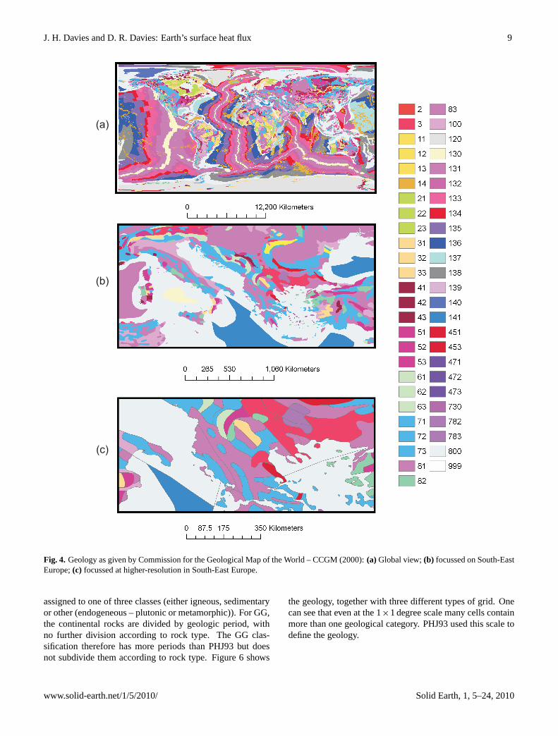
1. A global data-set, CCGM/CGMW (Commission for theGeological Map of the World, 2000), abbreviated toCCGM (the French initials for the data-set – Commis-sion de la Carte Geologique du Monde). It ascribes ev-ery point on Earth’s surface to a geological unit (seeFig. 4).

2. A data-set of continental geology (Hearn et al., 2003),abbreviated to GG – for Global GIS. It includes virtu-ally all land above sea-level, excluding Antarctica andGreenland (see Fig. 5).

The CCGM has 14 202 geology polygons, while the GGdata-set has 91 964 polygons. Therefore, GG has a muchhigher level of detail, especially in the USA. When usingthe GG data-set, the CCGM data-set is used for areas withno coverage (i.e. when the GG data-set is used, we also use1066 geology polygons from the CCGM data-set to representthe absent areas with heat flow observations – e.g. oceans).Table 1 presents the various 51 geology units in the CCGMdata-set, while Table 2 presents the 20 geology units in theGG data-set. Note that, compared to PHJ93, these data-setsuse a different division of geological units: PHJ93 repre-sented the geology using 21 subdivisions, where they subdi-vided the Cenozoic, Mesozoic and Paleozoic periods into ig-neous and others, but the Proterozoic, Archean and subaque-ous continental were all undifferentiated. When compared toPHJ93, the CCGM classification has only slightly more divi-sions of the oceanic domain. However, there are major dif-ferences on the continents, where CCGM has a finer divisionof geological time. In addition, the rocks of most periods are



(a)

(b)

(c)

Fig. 4. Geology as given by Commission for the Geological Map of the World – CCGM (2000):(a) Global view;(b) focussed on South-EastEurope;(c) focussed at higher-resolution in South-East Europe.

assigned to one of three classes (either igneous, sedimentaryor other (endogeneous – plutonic or metamorphic)). For GG,the continental rocks are divided by geologic period, withno further division according to rock type. The GG clas-sification therefore has more periods than PHJ93 but doesnot subdivide them according to rock type. Figure 6 shows

the geology, together with three different types of grid. Onecan see that even at the 1×1 degree scale many cells containmore than one geological category. PHJ93 used this scale todefine the geology.



Fig. 5. Geology (GG) as given by Hearn et al. (2003):(a) Global view(b) focussed on South-East Europe,(c) focussed at high-resolution inSouth-East Europe.

While we have already commented on the fact that thereis a strong variation in the density of heat flow observationswe should also note that there is a strong spatial variation inthe detail of geological classification provided by the digital

data-sets. This reflects the varying geological mapping thathas been undertaken in different regions of the world, in ad-dition to the intrinsic variability of global geology.



Table 1. Breakdown of the Geology in the Commission for the Geological Map of the World (2000), which we abbreviate to CCGM inthe text. Sed – sedimentary rocks (or undifferentiated facies); end – endogenous rocks (plutonic and/or metamorphic); arc – continental andisland arc margins; vol – extrusive volcanic rocks; SM – seamount, oceanic plateau, anomalous oceanic crust; OC – oceanic crust; undiff –undifferentiated.

Code Num. of Stratigraphy Lithology Total areaPolygons m2

100 824 Cenozoic – Quaternary Sed. 1.871E+1311 15 Precambrian (undiff.) Sed. 1.239E+1112 45 Precambrian (undiff.) Vol. 3.660E+10120 94 Glacier 1.439E+1313 138 Precambrian (undiff.) End. 3.950E+12130 489 Plio-Quaternary OC 1.613E+13131 292 Miocene OC 5.031E+13132 273 Oligocene OC 3.171E+13133 182 Eocene OC 3.763E+13134 221 Paleocene OC 2.105E+13135 87 Upper Cretaceous OC 4.547E+13136 44 Lower Cretaceous OC 3.459E+13137 16 Upper-Middle Jurassic OC 1.771E+13138 46 Age unknown OC 2.406E+13139 4 Neogene OC 4.548E+1114 1272 SM 2.184E+13140 1 Undiff. Cretaceous OC 1.171E+12141 3 Undiff. Jurassic - Cretaceous OC 6.290E+112 2 Proterozoic + Paleozoic (undiff) Vol. 4.374E+0921 74 Archean Sed. 3.748E+1122 106 Archean Vol. 4.141E+1123 495 Archean End. 7.246E+123 69 Precambrian + Paleozoic (undiff) End. 3.399E+1131 783 Proterozoic Sed. 6.754E+1232 123 Proterozoic Vol. 1.027E+1233 848 Proterozoic End. 1.168E+1341 704 Lower Paleozoic Sed. 8.191E+1242 27 Lower Paleozoic Vol. 1.395E+1143 281 Lower Paleozoic End. 5.743E+11451 40 Paleozoic (undifferentiated) Sed. 1.446E+11453 149 Paleozoic (undifferentiated) End. 1.345E+12471 41 Paleozoic + Mesozoic (undiff) Sed. 2.382E+11472 21 Paleozoic + Mesozoic (undiff) Vol. 8.199E+10473 15 Paleozoic + Mesozoic (undiff) End. 5.485E+1051 756 Upper Paleozoic Sed. 1.207E+1352 51 Upper Paleozoic Vol. 8.658E+1153 213 Upper Paleozoic End. 9.414E+1161 209 Triassic – Mesozoic Sed. 2.880E+1262 25 Triassic – Mesozoic Vol. 9.431E+1063 32 Triassic – Mesozoic End. 1.402E+1171 1080 Jurassic & Cretaceous – Mesozoic Sed. 2.033E+1372 275 Jurassic & Cretaceous – Mesozoic Vol. 3.239E+1273 636 Triassic – Mesozoic – Jurassic & Cretaceous End. 1.879E+12730 29 Age unknown End. 4.740E+10782 6 Meso-Cenozoic (undiff) Vol. 1.117E+10783 8 Meso-Cenozoic (undiff) End. 5.398E+10800 329 Arc 5.871E+1381 1203 Cenozoic Sed. 2.301E+1382 1192 Cenozoic Vol. 5.816E+1283 94 Cenozoic End. 4.284E+11999 240 Lake 9.616E+11

SUM 14202 5.101E+14



Table 2. Breakdown of the geology in Hearn et al. (2003), GlobalGIS (abbreviated as GG in the text).

Period Number of Total Area Number of heatpolygons (m2) flow measurements

Cambrian 2541 3.378E+12 160Carboniferous 3591 3.413E+12 349Cenozoic 486 2.431E+11 4Cretaceous 8492 1.287E+13 1661Devonian 3268 3.617E+12 353Eocene & Oligocene 39 2.122E+11 2Holocene 485 1.706E+11 26Jurassic 5376 5.394E+12 579Mesozoic 5200 3.536E+12 245Ordovician 1825 2.391E+12 200Paleozoic 7145 4.820E+12 681Permian 2463 3.421E+12 390Precambrian 11895 2.871E+13 1563Quaternary 12063 2.968E+13 2927Silurian 1558 1.723E+12 92Tertiary 18026 2.304E+13 6147Triassic 3463 4.537E+12 482Volcanic 442 7.290E+10 5Water/Ice 395 5.721E+11 87Undefined 3211 1.050E+12 380Total 91964 1.328E+14 16333

2.3 Grids

PHJ93 used a 1×1 degree equal longitude grid (64 800 gridcells) (see Fig. 6a for an example) in their analysis. Wehave undertaken our preferred analysis using a 1×1 degreeequal area grid, with 41 252 cells in total. These cells are1×1 degree at the equator, but at pole-ward latitudes the celllongitudes increase to approximate equal area. In this way,each cell has the same and equal weight (see Fig. 6b for anillustration of this grid in the North Atlantic). The differencebetween an equal area and equal longitude grid is greatest athigh latitudes. Since there are limited heat flow observationsat high latitudes, we expect that the improvement of usingan equal area grid might be limited in this study. Amongstour range of investigations we also used a 5×5 degree equallongitude grid (see Fig. 6c).

2.4 Analysis

To better illustrate the impact of various aspects of themethodology, we have undertaken a series of alternative anal-yses, giving us a handle on the level of uncertainty in ourestimate. We shall next describe, in detail, the methodologyused in our preferred analysis, since this is the most com-plex. This will allow us to more easily describe the otheranalyses, without having to repeat the complete descriptionof each stage:

(a)

(b)

(c)

Fig. 6. Presentation of CCGM Geology, focussed on the North At-lantic, together with 3 different grids:(a) 1 degree equal longitudegrid; (b) 1 degree equal area grid; and(c) 5 degree equal longitudegrid.

1. We plotted up all CCGM and GG geology. Wethen erased the GG geology from the CCGM geology(i.e. the areas covered by the GG data-set are removedfrom the CCGM data-set, such that recombining the re-sulting data-set with the GG data-set leads to completeglobal coverage, with no overlap).

2. The two resultant geologies were unioned with the1×1 degree equal-area grid. The union operation com-putes a geometric intersection of the input features; inthis case the geology layer and the grid layer. All fea-tures are output to a new layer, with the attributes ofboth input features. The result of this process is toproduce polygons that are the same or smaller thanthe original geology (and grid) polygons (see Fig. 7).The union process is undertaken to counter the strong



1 1

13

4

52

2

+ =

(a)

(b)

Fig. 7. The process of unioning:(a) We illustrate the union processwith two rectangles in the first layer and one circle in the secondlayer. Following union the resultant layer, in this case, has 5 poly-gons, none of which are circular or rectangular. We note that thenumber of polygon features in the output layer is greater than thenumber of polygons in either input layer. Any polygon on eitherinput layer can be made up from a number of polygons in the out-put layer. The resultant layer has the attributes ofboth input layerpolygons in its attribute table;(b) a schematic of how the processwould look for the grid and geology polygons.

clustering that exists in the heat flow data-set; by usingthe union methodology, large geologic regions do notget dominated by measurements from one heavily stud-ied site. It should be noted that both PHJ93 and Jaupartet al. (2007) (JLM07) utilise 1 degree equal longitudegrids to minimise the effects of clustering.

3. The resulting polygons were spatially joined to the heatflow data. In the spatial join, the attributes of the geol-ogy polygon containing the heat flow point is added tothe table of attributes of the heat flow points (i.e. eachheat flow point has its geology associated with it – seeFig. 8).

4. The mean heat flow for each geology polygon (unionedwith the grid as described above) was calculated, pro-ducing a new output (summary) table (see Fig. 9). Thegeology label of each polygon and the average heat flowwas stored in the summary table.

5. The mean heat flow value was calculated for each geol-ogy class using the summary table of the previous step.This, again, was a straightforward arithmetic mean ofall polygons that had non-zero heat flow polygons foreach specific geology.

6. The global area of each geological unit was calculated.

7. The final estimate of the global average heat flow wasevaluated by assuming that the average heat flow foundfor each geology could be assigned to all similar geol-ogy (i.e. for each geological category, its average heat

flow was multiplied by its global area to find its contri-bution to the global heat flux).

We follow JLM07 and PHJ93 and make an estimate for hy-drothermal circulation, assuming that the heat flow in youngoceanic crust is best described by a half-space model. Un-like PHJ93 who used the parameters of SS, we have used thevalue suggested by JLM07, but have also repeated the analy-sis using the parameters of Parsons and Sclater (1977) (here-after abbreviated to PS) and SS, to examine the differencesand uncertainties arising from these models. Thus, for allgeology younger than 66.5 Ma (66.4 Ma for 1983 timescale)we have replaced the heat flow obtained from the raw datawith a value obtained from the equation:

q = C/√

t (1)

where q is surface heat flux (mW m−2), C is a constant(mW m−2 Myr0.5), and t is the age of the oceanic litho-sphere in millions of years. The value ofC preferred byJLM07 is 490±20 mW m−2 Myr0.5; while the values of SSand PS are 510 and 430 mW m−2 Myr0.5, respectively. Theerror of JLM07 is small, partly because they use the con-straint that at infinite age the half-space model should pre-dict zero heat flux. While that is certainly correct, it mightbe over optimistic to believe that a half-space model with asingle constant is the correct model, at least as fit throughall the data selected over such a wide range. We note thatJLM07 ignore data at old age, since the half-space model isknown not to fit that data well (that miss-fit led to the devel-opment of plate models), and at very young age, since thehigh variability reduce their usefulness in constraining theparameters. As a result we take a slightly more conserva-tive estimate of the error inC and assume errors 50% greater(i.e.±30 mW m−2 Myr0.5 at 2 standard deviations).

Table 3 shows the results for the 56 individual geologyunits (the 20 units on the continents from GG, and the36 units from CCGM that represent the rest of the globenot included in the GG data-set) for this case. As describedabove, the final result is produced by multiplying the averageheat flow calculated for each geology by the global area forthat geology. Notice that some geological units have no (orvery few) heat flow measurements. However, these make uponly a very small proportion of the total area (1.5%, for lessthan 50 readings (excluding the Glacier category, which isdiscussed below and makes up∼3% of area)). For cases ofgeology with insufficient readings for the area to be included,we have shared the area among similar regions.

Taking the standard deviation of the heat flow values con-tributing to the estimate of a mean for a geological unit asthe basis for estimating the error in the mean, we find thatthe resulting errors, weighted by area, are small (i.e.±2.2and 3.0 mW m−2, for the GG and CCGM data-sets respec-tively, 2 std. dev.). There is, however, additional uncertainty,arising from: (i) the inaccuracy of the area; (ii) the fact thatthe extrapolating method is not perfect (i.e. the geology class



A

BC A

BC

Point

Polygon Polygon Attributes

Point Attributes

Point Attributes Polygon Attributes

A

A 1

B

B 1

C

C 2

11

2

2

SpatialJoin

Fig. 8. Schematic illustrating the spatial join between a layer with three points and a second layer of two polygons. The process adds theattributes of the appropriate polygon that contains the point of interest. This is how we assign a geology to each heat flow measurement.

Summariseon Geology

Original Table Summarised Table

Geology

GeologyMeanValue Frequency

FurtherAttribute

A

FurtherAttribute

B

FurtherAttribute

C

Heat FlowValue

A

A 3

1

1

B

C

56.2

59.57

78.7

33.767.6

54.9

33.7

78.7B

C

A

A

..... ..... .....

.....

.....

.....

..... .....

.....

.....

..........

.....

.....

.....

Fig. 9. Schematic illustrating the process of producing a summarytable. A target field is selected, in this case geology. The process“summarises” selected fields in defined manners e.g. mean, sum,standard deviation, that correspond to each unique entry in the se-lection field. In the example illustrated, the mean heat flow has beensummarised for each geology category. The summary table will alsocontain the number of rows (heat flow measurements) contributingto each summary value.

is not a perfect predictor of the heat flow); and (iii) the factthat large areas of Africa, Antarctica and Greenland are un-sampled. Errors in the area could arise due to poor definitionof geological boundaries in the digital geology maps. We donot estimate such errors here. However, we find that our es-timate of continent (ocean) area is slightly greater (less) thanJLM07, but as JLM07 point out, since the total area is fixed,these differences have only a small effect. The issue of theinadequate extrapolation and the poor coverage is more sig-nificant as a source of error and is later discussed in detail.

We have decided to include a value for the Glacier cate-gory in our preferred analysis. The Glacier category of theCCGM geology covers 3% of Earth’s surface area, primarilyacross Greenland and Antarctica. Depending upon the ex-act methodology used, we get between 2 and 5 final readings(grid, geology), and a mean heat flow value of between 105and 120 mW m−2, which is probably far too high a value. Anestimate of 65 mW m−2 was recently made for the heat fluxin Antarctica, from estimates of the depth to the Curie tem-perature, based upon magnetic field measurements (Maule etal., 2005). The work of Shapiro and Ritzwoller (2004) alsorefers to the problem of estimating the heat flow of Antarc-

tica, in this case using seismic measurements as a proxy.They suggest that the heat flow in West Antarctica is almost afactor of three higher, and more variable (more like the smallnumber of actual heat flow observations in our data-set), thanin East Antarctica, where the heat flow has an estimated “lo-cal mean” of 57 mW m−2. Since East Antarctica has a largerarea than West Antarctica (by a factor of∼3), the work ofShapiro and Ritzwoller (2004) would also argue for an over-all value for Antarctica closer to 65 mW m−2 rather than the∼105–120 mW m−2 given by the raw measurements. Whilethis is similar to current predictions of the average heat flowthrough continents, it must be viewed as an uncertain esti-mate. However, our preference is to use this estimate and(105–65) mW m−2 as the two standard deviation estimate ofthe error (105 mW m−2 being the minimum direct estimatefrom the data).

In Table 4 we list the heat flow and geology data-sets, thegrids, and the methods used for the various alternative anal-yses undertaken. Each case is next described in detail:

1. While we have not repeated the work of PHJ93, in ourfirst analysis, we used their heat flow data-set (takenfrom Gosnold and Panda, 2002), a 5× 5 degree equallongitude grid and their methodology of selecting geol-ogy for the whole of a cell, based on the majority geol-ogy of that cell. However, we used the CCGM geologydata-set.

2. As in Case 1, but using the new heat flow data-set(DD10).

3. As in Case 2, but a spatial join was undertaken betweenthe heat flow data and the underlying geological poly-gons.

4. As in Case 3, but, in addition, we undertook a unionbetween the geology and a 1 degree equal area grid.

5. As in Case 3, but with the combination of GG andCCGM geology data-sets.

6. The preferred analysis described above.



Table 3. Detailed breakdown of the preferred analysis for Earth’s surface heat flux. The raw data yields heat flow estimates of 105–120 mW m−2 for the Glacier category (113.5 mW m−2 in the preferred analysis); the value of 65 mW m−2 listed here comes from Maule etal. (2005), with the error estimate based on the difference between 105 and 65 mW m−2. The raw total, with no young ocean crust heat flowestimate, is 36.0 TW. The total over the GG geology is 9.2 TW. The total over the non-GG geology, including the young ocean estimate is36.4 TW, while 36.6 TW is the value after allowance is made for ignoring geology classes with<50 readings. Therefore, the final estimate,including the young ocean estimate, is 45.6 TW (or 45.7 TW, ignoring geology classes with<50 readings). Adding 1 TW for the effect ofhot-spots on young oceanic crust yields a final total of 46.7 TW.

PERIOD Number of Number of Avg. Std. Error in Total Totalpolygons with heat flow Heat Flow Dev. the mean Heat Flow correctedheat flow data obs. (mW m−2) (mW m−2) (TW) heat flow (TW)

Cambrian 87 160 50.5 23.6 2.0 0.170 0.170Carboniferous 206 349 71.9 161.9 6.8 0.245 0.245Cenozoic 3 4 49.2 18.6 9.5 0.012 0.012Cretaceous 672 1661 66.7 35.9 1.3 0.858 0.858Devonian 172 353 52.5 21.3 1.2 0.190 0.190Eocene & Oligocene 2 2 72.5 48.8 34.5 0.015 0.015Holocene 12 26 54.4 17.3 3.4 0.009 0.009Jurassic 266 579 64.1 36.3 4.0 0.346 0.346Mesozoic 141 245 68.7 38.5 2.3 0.243 0.243Ordovician 103 200 54.1 34.1 2.5 0.129 0.129Paleozoic 352 681 67.5 37.5 2.0 0.325 0.325Permian 122 390 57.7 21.6 0.9 0.197 0.197Precambrian 698 1563 59.9 55.5 1.5 1.720 1.720Quaternary 901 2927 82.0 103.2 6.5 2.435 2.435Silurian 53 92 53.9 20.9 2.4 0.093 0.093Tertiary 1660 6147 77.3 121.8 1.7 1.781 1.781Triassic 187 482 68.1 53.5 2.3 0.309 0.309Volcanic 5 5 39.0 10.1 4.5 0.003 0.003Water/Ice 12 87 58.4 21.4 3.2 0.033 0.033undefined 117 380 53.4 22.4 1.1 0.056 0.056

Sum over GG 5771 16 333 9.17 9.17

Glacier 1 2 65.0 0.0 20.0 0.92 0.92Plio-Quaternary OC 424 4397 132.6 102.9 5.00 2.139 6.847Miocene OC 826 3408 78.2 60.6 2.11 3.934 6.936Oligocene OC 361 1063 66.3 74.3 3.91 2.103 2.926Eocene OC 430 988 62.8 43.0 2.08 2.363 2.774Paleocene OC 266 652 61.0 28.5 1.75 1.284 1.326Upper Cretaceous OC 531 1571 66.8 52.8 2.29 3.036 3.036Lower Cretaceous OC 452 1399 61.1 48.6 2.29 2.114 2.114Upper-Middle Jurassic OC 304 1107 54.0 28.9 1.66 0.956 0.956Age unknown OC 266 642 71.5 51.4 3.15 1.720 2.270Neogene OC 15 29 127.6 36.4 9.40 0.058 0.093Seamount, oceanic plateau, anomalous oceanic crust 319 993 73.8 107.5 6.02 1.610 1.610Undifferentiated Cretaceous OC 12 58 54.8 4.3 1.25 0.064 0.064Undifferentiated Jurassic – Cretaceous OC 40 224 34.2 18.9 2.99 0.020 0.020Continental and island arc margins 1002 4556 73.8 91.1 2.88 4.242 4.242Lake (not in the legend) 46 618 64.1 71.8 10.59 0.045 0.045Cenozoic – Quaternary Sed. 26 40 72.1 19.5 3.83 0.019 0.019Precambrian (undifferentiated) End. 1 1 46.0 n/a 0.00 0.003 0.003Archean Ext 1 4 23.0 n/a 0.00 0.000 0.000Precambrian + Paleozoic (undifferentiated) End. 2 3 74.7 16.6 11.71 0.001 0.001Proterozoic Sed. 3 6 51.2 10.7 6.20 0.017 0.017Proterozoic Ext. 1 2 43.5 n/a 0.00 0.003 0.003Proterozoic End. 12 31 51.5 19.4 5.59 0.030 0.030Lower Paleozoic Sed. 13 17 62.7 29.2 8.09 0.020 0.020Paleozoic (undifferentiated) Sed. 1 0 0.0 n/a 0.00 0.000 0.000Paleozoic (undifferentiated) End. 4 5 60.5 32.2 16.10 0.008 0.008Upper Paleozoic Sed. 13 17 52.5 14.8 4.11 0.015 0.015Upper Paleozoic Ext. 1 1 46.0 n/a 0.00 0.002 0.002Upper Paleozoic End. 3 3 69.3 31.2 18.02 0.002 0.002Triassic – Mesozoic Sed. 3 7 36.6 22.6 13.05 0.003 0.003Jurassic & Cretaceous – Mesozoic Sed. 34 73 64.7 35.5 6.09 0.026 0.026Jurassic & Cretaceous – Mesozoic Ext. 4 9 39.3 11.0 5.50 0.014 0.014Triassic – Mesozoic – Jurassic & Cretaceous End. 4 4 49.0 31.6 15.82 0.009 0.009Age unknown End. 2 2 77.5 23.3 16.50 0.000 0.000Cenozoic Sed. 32 66 67.2 27.3 4.83 0.024 0.024Cenozoic Ext. 13 16 102.4 29.0 8.04 0.040 0.040

Total over non-GG 5468 22 014 26.85 36.42/36.63

TOTAL 11 239 38 347 36.0 45.6/45.7

FINAL TOTAL +1 TW for hot-spots 46.7on young oceanic crust



Table 4. Description of the various analyses undertaken. 5 deg eqlon; a grid with 5 degree spacing in longitude. 1 deg eq area; a gridwith 1 degree spacing in longitude at the equator, but varying longi-tude at other latitudes to maintain an equal area. Majority Geology;the geology which takes up the greatest area inside the grid cell isascribed to the whole grid cell. These and other aspects related tothis table, including union, are described further in the text.

Analysis Data-set Geology Grid Geology polygons

1 Pollack CCGM 5 deg equal lon Majority geology2 DD10 CCGM 5 deg equal lon Majority geology3 DD10 CCGM None Original polygons4 DD10 CCGM 1 deg equal area Union with Grid5 DD10 CCGM/GG None Original polygons6 DD10 CCGM/GG 1 deg equal area Union with Grid

3 Results

In Fig. 10, we plot the heat flow map of the world fromour preferred analysis. The standard error (2 std. dev.) forthe heat flow ascribed to each geological unit is presentedin Fig. 11. We note that the error is highest for the youngocean estimates and the Glacier domains. Of course, theseestimates of error are not useful locally; for example, someparts of Africa have no measurements. Therefore, like thevalue on the Global heat flow map being only indicative forthat geology unit, likewise the error.

Results from the various cases examined are listed in Ta-ble 5. One can see that the raw global heat flow in each casevaries from 35.8 to 36.7 TW, with our preferred analysis giv-ing a value of 36.7 TW. After the Stein and Stein (1992) SS-based young ocean estimate, one gets values ranging from44.1 to 47.2 TW, with 47.2 TW for our preferred analysis;or 40.7 to 43.5 TW using the Parsons and Sclater (1977) PS-based estimate (43.4 TW for our preferred analysis). We notethat the difference between estimates using only the raw data,and those using the SS half space model can vary between 7.8and 11.1 TW, with a difference of 10.5 TW for our preferredanalysis. We also note that using the SS and PS models leadsto a difference of 3.4 to 3.8 TW (3.8 TW preferred analysis).Our preferred correction is between those of PS and SS, giv-ing a total heat flow value of 46.7 TW.

The preferred analysis can be divided into four compo-nents (see Table 6): (i) young oceans; (ii) the rest of theoceans and continents; (iii) the Glacier category; and (iv) thecontribution from hot-spots. Each is next described in detail.

1. Our estimate for heat flow in young oceans produces23.1 TW (128 mW m−2), compared to the 24.5 TW ofPollack et al. (1993) (PHJ93) (based on SS). Jaupart etal. (2007) (JLM07), whose value ofC we have adopted,give 24.3 TW (the differences between our estimate andthat of JLM07 arise from: (i) variations in the areasof geological units; (ii) the division of geologic time;

and (iii) the fact that ours covers oceanic crust out to66.5 Ma while JLM07 extends out to 80 Ma), whileWei and Sandwell (2006) give a value of 20.4 TW. ThePS model, with our area, leads to a young ocean heatflow estimate that is 2.8 TW less than that adopted here,while the SS model gives a value 1 TW greater. Con-sidering the PS-model estimate might be too low, it isclear that an uncertainty of∼2 TW is suggested by thealternative analyses listed above; our assumption thatthe error inC is ±30 mW m−2 Myr0.5 at 2 standard de-viations, gives this component an error of±1.3 TW.

2. Estimates obtained for the rest of the oceans andcontinental components depend upon: (i) the fun-damental assumption of a correlation between heatflow and geology; and (ii) the use of a 1 degreeequal area grid to reduce the influence of clus-tering. Our preferred analysis predicts values of13.8 TW/73 mW m−2 (continents), 7.8 TW/66 mW m−2

(rest of oceans); for this component of the heat flow.This compares to 13.2 TW/65 mW m−2 (continents),7.6 TW/56.4 mW m−2 (rest of oceans) from PHJ93 and14 TW/65 mW m−2 (continents), 4.4 TW/48 mW m−2

(>80 Ma) from JLM07. A significant percentage ofthe increased global heat flux in this study thereforearises due to this component, suggesting that heat flowvalues recently added to the global heat flow data-sethave been, on average, slightly higher than earlier val-ues (as illustrated in the histogram of the raw data ofFig. 3b). This continues the slight upward trend in theestimate for global heat flux over recent years (see Ta-ble 4 PHJ93, and JLM07).

3. As described above, for the Glacier category we haveused a value of 65 mW m−2 based on the depth tothe Curie temperature found from undertaking a spec-tral analysis of aeromagnetic data (Maule et al., 2005),rather than the very small (2 to 5) measurements that fallwithin this category in the various analyses (the raw datagives heat flow estimates of 105 to 120 mW m−2 for thevarious analyses – 113.5 mW m−2 in the preferred anal-ysis). This gives a value of 0.9±0.3 TW. We note thatusing this alternative value for Antarctica (and Green-land), rather than the raw heat flow measurements, canmake a difference of between 0.7 and 1.0 TW (0.7 TWin our preferred analysis). PHJ93 do not really addressthis issue while JLM07 include it in their total continen-tal area and effectively use the global average, whichis 65.3 mW m−2. JLM07 include the error from thiscomponent in their total error estimate (for continents),which is 1 TW.

4. Hot-spot regions typically do not exhibit higher heatflow values compared to that expected for their crustalage, excluding a few sites at or near volcanic fea-tures (Stein and Von Herzen, 2007). Nonetheless,



(a)

(b) (c)

75 - 85

85 - 95

95 - 150

150 - 450

23 - 45

45 - 55

55 - 65

65 - 75

Fig. 10. (a)Map of the preferred global heat flux (mW m−2), utilising the underlying estimates for each geology category. Note that inregions with no data (see Fig. 1) the estimate is based solely on the assumed correlation between geology and heat flux. As a result, locally,the values presented could provide a poor estimate. Estimates in better-covered areas of the globe, however, suggest that on average, thecurrent estimates are robust; higher resolution plots, focussing upon Europe(b) and Japan(c) are also shown.



0 - 5

5 - 10

10 - 15

15 - 30

30 - 60

Fig. 11. Map of the estimated error in the preferred global heat flux (mW m−2). The error is based on the actual spread of heat flow valuesfor each geology category, with the exception of regions where the heat flow value is based on calculation (young oceanic crust) and theGlacier category (for more details see text). The mapped error does not include the component from hot-spots or the uncertainty in the areaof geology polygons. We note that the largest error is related to the young oceanic crust and the glacier category.

JLM07 include a contribution for hot-spots in their anal-ysis, which they argue are not accounted for in theirmethod. They estimate that this contribution is between2 and 4 TW globally, based on Davies (1988) and Sleep(1990); with an error of±1 TW. In our estimate forheat flow across young oceanic crust, we assume thatthe calibration measurements for the models have beenselected to avoid hot-spots and, therefore, the effect ofhot-spots is not included (thus a correction is needed).In contrast, we feel that hot-spot anomalies are includedin the rest of the measurements on the ocean floor andcontinent. As a result, we only include a hot-spot cor-rection for the young oceanic domains, which is propor-tional to the surface area included in the young oceanestimate. We take a contribution of 1±0.33 TW.

As mentioned above, some geology classes have very fewheat flow measurements. We have looked at limiting our es-timates to only geology classes with: (i) at least 5; and (ii) atleast 50 readings. Such a change has only a small effect onthe final global estimate, of order±0.3 TW (see Table 5).However, the random errors are reduced substantially by re-stricting the analysis to geology classes with at least 50 read-ings, although the errors in the young ocean estimates aremuch higher. This is because geology classes with less than50 readings cover only a small percentage of Earth’s surface.Indeed, the remaining classes (i.e. with>50 readings) cover

>96% of Earth’s surface. Our preference is to ignore ge-ology classes with<50 readings. Our final preferred valueis 46.7 TW, with an error of 2 TW (2 standard deviations).To be consistent with our error estimate of±2 TW we round46.7 to 47 TW. This final preferred estimate is separated intothe oceanic and continental realms in Table 7.

4 Discussion

In this section we primarily focus on various components thatlead to the uncertainty (±2.0 TW) in our final estimate. As-pects considered include: (i) the fundamental correlation as-sumed between geology and heat flow; (ii) potential issueswith the heat flow data, including the raw measurements andthe areal coverage of the data-set; (iii) the implications of thevarious methods undertaken; (iv) issues related to hydrother-mal corrections in oceanic crust; (v) hydrothermal circulationon continents; (vi) the glacier category; and (vii) combiningstatistical errors. We end by discussing the implications ofour preferred value of 47 TW.



Table 5. The total global surface heat flux from the various analyses undertaken. Note that the first row of results is from Pollack et al. (1993).Pollack is used as an abbreviation for the heat flow data-set, the geology and the method of using geology, used in Pollack et al. (1993). SS –Stein and Stein (1992); PS – Parsons and Sclater (1977); S. Join – spatial join; 1×1 long – 1 degree by 1 degree equal longitude grid; 1×1area – 1 degree by 1 degree equal area grid; CCGM – Commission Geology Map of World (2000); GG – Global GIS (2003); DD10 – thedata-set presented in this paper. The original version was provided by Laske and Masters (pers. comm.) and DD10 has only minor changes.See text for further explanation of terms and abbreviations used in table.

Cas

enu

mbe

rfr

omTa

ble

4

Sou

rce

ofH

eatF

low

Dat

aset

Geo

logy

Grid

How

isge

olog

yus

ed?

Tota

lHea

tFlo

w–

(TW

)–

data

base

d

Tota

lHea

tFlo

w–

with

pref

erre

dyo

ung

Tota

lHea

tFlo

w–

with

SS

Diff

eren

cebe

twee

nra

wda

ta

Tota

lHea

tFlo

w–

with

PS

Diff

eren

cebe

twee

nS

San

dP

S

Tota

lHea

tFlo

ww

ithS

Ses

timat

ebu

tass

um-

Diff

eren

cebe

twee

nor

igin

alan

das

sum

-

Tota

lHea

tFlo

w–

with

SS

estim

ate

(TW

)

Tota

lHea

tFlo

w–

with

SS

estim

ate

(TW

)

Ant

arct

ica

and

ocea

n

ocea

ncr

uste

stim

ate

(TW

)an

dho

t-sp

ot

base

des

timat

e(T

W)

and

SS

estim

ate

(TW

)

base

des

timat

e(T

W)

estim

ates

(TW

)

ing

65m

Wm−

2fo

rA

ntar

ctic

a(T

W)

ing

65m

Wm−

2fo

rA

ntar

ctic

a(T

W)

–ex

clud

ing

geol

ogie

sw

ith<5

read

ings

–ex

clud

ing

geol

ogie

sw

ith<50

read

ings

PHJ93 Pollack Pollack 1×1 long Pollack avg 33.51 44.20 10.691 Pollack CCGM 5×5 long Pollack avg 36.25 44.06 7.81 40.68 3.38 43.08 0.98 43.39 43.422 DD10 CCGM 5×5 long Pollack avg 36.26 44.09 7.83 40.71 3.38 43.11 0.98 43.43 43.453 DD10 CCGM None S. Join 35.83 45.86 10.03 42.16 3.70 45.27 0.59 45.63 45.404 DD10 CCGM 1×1 area Union 36.14 47.06 11.08 43.35 3.71 46.46 0.60 46.75 47.035 DD10 CCGM + GG None S. Join 37.17 47.20 10.03 43.50 3.56 46.51 0.69 46.93 46.986 DD10 CCGM + GG 1×1 area Union 36.71 46.68 47.23 10.52 43.44 3.79 46.54 0.69 46.99 47.13

Table 6. The preferred analysis of Earth’s surface heat flux, broken down into five categories: (i) continents from data; (ii) oceanic crustcontribution by calculation (age<66.5 Myr); (iii) oceanic crust from data (age≥66.5 Myr); (iv) the glacier category; and (v) the hot-spotcontribution. Columns of alternatives are also presented. “+1” signifies that this answer uses a 1-degree equal-area grid through a “union”, toreduce the influence of clustering. “50” means that only geology categories with at least 50 heat flow measurements were used in this answer.GG – Global GIS geology (Hearn et al., 2003); CCGM – CCGM geology (Commission for the Geological Map of the World, 2000); PHJ93– result from Pollack et al. (1993) (breakdown calculated by combining information in their Tables 2 and 3); JLM07 – result from Jaupart etal. 2007). C510, C490, C430 – estimation using C values in Eq. (1) of 510, 490 and 430 mW m−2 Myr0.5, respectively (SS – Stein and Stein(1992), whereC was 510 mW m−2 Myr0.5; PS – Parsons and Sclater (1977), whereC was 430 mW m−2 Myr0.5); WS – result for oceaniccrust heat flow younger than 66 Myr from Wei and Sandwell (2006); 1983 T.S. – the 1983 Geological Time Scale (Palmer, 1983). Maule etal. (2005) is the estimate of Antarctica’s heat flow from Maule et al. (2005). Preferred total = 13.77 + 23.14 + 7.84 + 0.92 + 1.00 = 46.67 TW.

Continents (TW) Young Ocean Estimate (TW) Rest of Oceans (TW) Glacier (TW) Hot-spots (TW)

GG+CCGM+1; 50 13.8 CCGM, C510, 24.1 CCGM+1; 50 7.8 Raw data, CCGM +1 1.6 PHJ93 0.0GG; 50 9.8 CCGM, C490, 23.1 CCGM; 50 8.3 Maule et al. (2005) 0.9 JLM07 3.0CCGM+1; 50 13.0 CCGM, C430, 20.3 CCGM + 1 7.8 DD10 1.0CCGM; 50 14.0 CCGM, C490, A (Eq. 3) 24.4 CCGM 7.8GG+CCGM+1 13.7 PHJ93 (<66.4 Myr) 24.5 PHJ93 (>66.4 Myr) 7.6GG 9.8 JLM07 (<80 Myr) 24.3 JLM07 (>80 Myr) 4.4CCGM+1 13.0 WS (<66 Myr) 20.4CCGM 14.2 CCGM, C490, 1983 T.S. 22.9PHJ93 13.2JLM07 14.0

Preferred 13.8 23.1 7.8 0.9 1.0



Table 7. Summary of continental and oceanic heat flow from ourpreferred estimates.

Area Heat Flow Mean Heat Flow(m2) (TW) (mW m−2)

Continent 2.073×1014 14.7 70.9Ocean 3.028×1014 31.9 105.4Global Total 5.101×1014 46.7 91.6

0

40

80

120

0 5 10 15 20 25

Square Root of Age (Myr0.5)

Mean

Heat

Flo

w(m

Wm

-2)

Fig. 12. A plot of the average heat flow for each geology categoryas a function of the square root of its mean age. There is a trend inthe data, of decreasing mean heat flow with increasing age. If oneexcludes the very oldest datum (the Archean – which stretches overa very long geologic age) and the very youngest data (these cate-gories have very few measurements), there is a strong correlation.While the correlation of heat flow with geology could apply withouta correlation between mean heat flow and age; the fact that such acorrelation exists does lend some support that this fundamental as-sumption might have some merit. The correlation is strong enough(R2 = 0.75) that it certainly seems better to take it into account thanignoring it.

4.1 The robustness of the fundamental correlationassumed

The fundamental correlation assumed by Pollack etal. (1993) (PHJ93) is that regions of similar geology have, onaverage, similar values for heat flow. From Table 3, one cansee that the standard deviation on the mean values for variousgeology categories is very high, suggestive that this assump-tion is not useful. However, this is misleading. In Fig. 12,we plot the mean heat flow of different geology categories asa function of the square root of age, for all categories withgreater than 50 measurements (the age for the Precambrianis hard to set; most of the measurements are likely to be inthe Late Proterozoic, but we have no way of knowing theexact age distribution. As a result, the Precambrian cate-gory is excluded from our plot). Polyak and Smirnov (1968)

were among the first to suggest such a relationship, whileMorgan (1985) pointed out that the relationship is weak.This weak relationship can be easily understood; althoughthere is evidence of some decrease in heat production withage, the range of heat production within each age group isgreater than the differences between age groups (Jaupart andMareschal, 2003, 2007). Nevertheless we find that there is aclear correlation in the data, with the average heat flow de-creasing with increasing age (R2 = 0.75). This implies thatthere is some power in the correlation and that using sucha methodology as an empirical estimator for un-sampled re-gions gives a better estimate (with slightly lower error) thana straightforward global average (as was done by Jaupart etal. (2007) (JLM07)). We remind readers that our assumptionis that there is a correlation on average between geologicalcategory (not necessarily age) and heat flow. It should alsobe noted that our final estimate and that of JLM07 are simi-lar. The relationship between average age and heat flow forthe continents with our data (excluding the Precambrian) is:

q = 102−2.25√

t (2)

whereq represents heat flow (mW m−2) andt is the age (mil-lions of years). We note that the thermo-tectonic age mightlead to a further improved correlation. However, at the timeof writing, such information was not available for the digitalgeologies used here.

Using this fundamental correlation, we find that the stan-dard error on each geology category is low, since our data-setcontains a large number of individual measurements. As aconsequence, the contribution of this to the final error is verysmall (note that the errors are area weighted, as is the globalestimate). However, since the correlation (between geologyand heat flow) is not perfect, the error in areas with very fewmeasurements could potentially be higher. As a result, it islikely that our estimate for this component of the error is un-realistically low. Nonetheless, once one realises that: (i) thespread of continental and old oceanic heat flow values havea limited range; and (ii) the uncovered area is not that great(at least at a 5 degree sampling), it cannot be very large. Theonly way to confirm our prediction is to continue measuringheat flow, especially in currently un-sampled areas.

4.2 The raw heat flow data

4.2.1 Measurement techniques

Heat flow readings are most robust when taken in deep bore-holes. However, such boreholes are rare and their construc-tion is expensive. Since the surface heat flux is small com-pared to the solar heat flux and the resulting advected heatby fluids through the near surface is large, it is always achallenge to obtain accurate estimates. The issues relatedto the collection of heat flow data are discussed in detail byBeardsmore and Cull (2001) for example, while Slagstad etal. (2009) illustrate a recent example of a leading edge study



that undertakes correction of heat flow measurements basedupon climate and topography (note that such modern correc-tions are likely very rare in the data-set used here). Whileobtaining more accurate heat flow measurements is essentialin constraining the global surface heat flux, we must acceptthat this will be a slow and expensive process. In the mean-time, as much as possible must be extracted from the mea-surements made to date.

4.2.2 Areal coverage of heat flow measurements

If we assume that the young ocean is well covered, since itis estimated from a model independent of our heat flow data,then at a 5 degree equal area grid sampling we find nearly84% coverage; at 1 degree equal area spacing we have 53%coverage. The coverage is not very much more than PHJ93(who had 62% coverage on a 5×5 degree grid), even thoughour data-set contains around 55% more heat flow measure-ments. This demonstrates that recent measurements added tothe data-set were made in similar geographical locations tothose in the data-set of PHJ93. Further measurements mustbe made in un-sampled regions to improve the reliability ofglobal heat flow estimates.

4.3 Various analysis choices

We have undertaken various analyses using different meth-ods and data-sets (see Tables 4, 5 and 6). Such a rangeof analyses allows us to evaluate that: (i) the effect of in-cluding alternative geology is between 0.1 and 0.2 TW (seeTable 5, 5th versus 7th row); (ii) not including the 1 degreegrid increases clustering and leads to a decreased heat flowof ∼0.15 TW (Table 5, last two rows); (iii) increasing thethreshold of points required to include a geology, as dis-cussed in Sect. 3, only changes the global heat flow slightly,but reduces that (small) component of the error; and (iv) thegeological time scales used give heat flow estimates that dif-fer by 0.2 TW (see Table 6, 2nd column, 23.1–22.9 TW),which is very small (we utilised the 2004 Geological TimeScale (Gradstein et al., 2005) for our preferred estimate. The1983 Geologic Time Scale (Palmer, 1983) was used for allother estimates). These analyses demonstrate that the finalresult is not sensitive to the details of these choices. In con-trast, the various analyses undertaken show that the youngocean estimate is a major contributor to the final error.

4.4 Hydrothermal correction in oceanic crust

It is well known that measurements of heat flow on youngoceanic crust grossly underestimate the actual heat flow(Davis and Elderfield, 2004). This is due to relatively shal-low hydrothermal circulation. Theoretically, heat flow is ex-pected to decline as the inverse square root of oceanic crustalage (Eq. 1). Indeed, this trend is observed in heat flow dataover old oceanic crust. Therefore, in obtaining a complete

estimate of Earth’s surface heat flux, one must correct for hy-drothermal circulation in young oceanic crust, using Eq. (1).A value for the constant C must therefore be selected and onemust know the distribution of ocean floor area as a functionof age. We note also that the theoretical expression cannotapply at the very youngest age. We discuss these aspects inturn.

4.4.1 TheC constant

As noted previously, estimates of the constantC vary; 430,490 and 510 mW m−2 Myr0.5, for PS, JLM07 and SS, re-spectively (note that these values are not strictly equiva-lent; JLM07 avoided hot-spots when calibrating data, butSS did not – in Table 5 we therefore do not include thehot-spot correction for the SS and PS cases. We have in-vestigated the influence of this constant on the total youngocean estimate by using all three values; the difference,bounded by the PS and SS values, is 3.8 TW. This is sig-nificant compared to other sources of uncertainty. Our pref-erence for C is the value of JLM07 (490 mW m−2 Myr0.5),although, as discussed in Sect. 2.4, we specify a larger un-certainty (30 vs. 20 mW m−2 Myr0.5). This increased uncer-tainty leads to a range of 2.6 TW, which is large, but less thanthe PS-SS range quoted above.

4.4.2 Area/age distribution

The estimate for heat flow in young oceanic crust is calcu-lated by multiplying the average heat flow for a certain agerange by the total area for that age. As a consequence, varia-tions in the estimate of area for different age ranges could besignificant. Table 1 lists the area of oceanic crust for CCGMgeology. While using the listed area is the best approach, inthis section we consider an alternative to get a sense of howsignificant this effect might be. JLM07, following Sclater etal. (1980) suggest that

dA

dτ= CA(1−τ/τm) (3)

whereA is the area of oceanic crust (km2), τ is the ageof the oceanic crust (years), andCA and τm are con-stants. In Fig. 13, we plot cumulative area as a functionof age, using the 2004 Geology Timescale, finding that itis well fit by the above expression (R2 = 0.98). We findCA = 3.7 km2 yr−1 while τm = 150 Myr. This compares to es-timates ofCA = 3.45 km2 yr−1 andτm = 180 Myr (Sclater etal., 1980) andCA = 3.34 km2 yr−1 (JLM07). If we use thearea given by Eq. (3), we get an estimate of 25.0 TW for theyoung oceans (for all ocean floor<66.5 Ma), compared to22.3 TW from a calculation using the actual areas. Using theconstants from JLM07 in Eq. (3), in an estimate of heat fluxout to age of 66.5 Ma, yields a value of 23.4 TW. Thereforethis source of error is∼1-2 TW at most, with a smaller errorlikely with using actual area as done in this work.



0.00E+00

1.00E+14

2.00E+14

3.00E+14

0 30 60 90 120 150 180

Age (Myr)

Area

(m

2)

Fig. 13. Cumulative area of oceanic crust (m2) as a function of age(Ma). A least squares fit through the data for Eq. (3) is shown as adark curve. We note that the data are reasonably well fit by such anexpression, as pointed out originally by Sclater et al. (1980).

4.4.3 Correction in very young oceanic crust

The half space formulation has a singularity (infinite value) atthe ridge axis (see Eq. 1). This is an integrable singularity soit causes no numerical problems. Davies et al. (2008) mod-elled the surface heat flow across a spreading ridge in a two-dimensional adaptive finite-element model. The model useda prescribed kinematic spreading upper surface to mimic thehalf space assumptions but avoided the unrealistic boundarycondition at the ridge and had the resolution to numericallyresolve the sharp variation. For a medium spreading rate of5 cm yr−1, Davies et al. (2008) found that the heat flow curvedeviates from the half space curve at around 0.15 Myr andwith an asymptotic value of just over 1 Wm−2. If these con-ditions were the weighted average conditions for all spread-ing ridges, the half-space model would overestimate the heatflow by around 0.1 TW. The overestimate would be locallygreater for slower spreading ridges and less for faster spread-ing ridges. While this effect is not negligible, it is less thanthe estimated error and, hence, we have not considered it inour final error estimate.

4.5 Hydrothermal circulation on continents

Since hydrothermal circulation is critical to estimates ofoceanic heat flux, it is sensible to enquire what role it mightplay on continents. JLM07 suggest that the contribution islikely to be small, given that the estimate for the entire Yel-lowstone system is around 5 GW, with similar values pre-dicted for the East African Rift. As stated by JLM07, itwould require 200 “Yellowstones” to increase the continen-tal heat loss by 1 TW. Our current understanding suggeststhat the contribution from this component is less than the es-timated error.

4.6 Glacier category

The error arising from the Glacier category is potentiallyvery large. As discussed earlier, our preference is a valueof 65 mW m−2 (Maule et al., 2005). The error bounds of theauthors (∼24 mW m−2) leads to an uncertainty of∼0.3 TW(0.9× 24/65), which is similar to our assumed error. Wenote that JLM07 estimate the error due to poor sampling tobe around 1 TW; effectively this combines the error from:(i) the poor sampling discussed earlier; and (ii) the error aris-ing from the Glacier category. Our weighted combined esti-mate for these sources of error is 0.8 TW.

4.7 Combining statistical errors

Our final estimate of the total area weighted error is 2 TW.This is slightly higher than the estimate of PHJ93 since wehave assumed more uncertainty arising from the young oceanestimate (and not ignored the uncertainty arising from poorlysampled categories – in this case arising from the “Glacier”category). It is 1 TW less than the error estimate of JLM07,even though our estimates of the error for individual com-ponents are similar. We estimate a contribution of: 1.3 TW(oceanic correction); 0.3 TW (Glacier category, which is re-lated to poor continental sampling in JLM07); 0.5 TW (restof oceans); 0.3 TW (rest of continents – CCGM); 0.4 TW(rest of continents – GG); and 0.3 TW (hot-spots). Assum-ing that these error terms are independent and uncorrelated,the combined uncertainty is only 2 TW (not 4 TW if one in-correctly added the error contributions naively (e.g. forA =

B +C, the errors should be combined1A2= 1B2

+1C2,not 1A = 1B +1C)). The biggest difference between ourerror and that of JLM07 is that we account for only 0.33 TW,compared to 1 TW, for the hot-spot correction.

4.8 Significance of result to thermal budget and thermalevolution models

Of the heat emerging at Earth’s surface (estimated at 47±

2 TW herein), it is believed that 6–8 TW is generated withinthe crust (e.g. Rudnick and Fountain, 1995; Jaupart andMareschal, 2003). It is argued that 5–13 TW originateswithin the core (e.g. Buffett, 2003; Lay et al., 2006), althoughthis range remains highly uncertain. The remainder (24–38 TW) must be provided by heat generation within the man-tle and by the secular cooling of the planet (plus minor con-tributions from other sources). Various models for the bulksilicate Earth (which includes the continental crust) lead to atotal present-day heat production of∼20 TW, with an uncer-tainty of∼15% (e.g. McDonough and Sun, 1995; Palme andO’Neill, 2003; Lyubetskaya and Korenaga, 2007b). Remov-ing the contributions from continental crust leaves a mantleheat production of 13±4 TW (JLM07). This would leave thebalance (7–29 TW) attributable to secular cooling. Recentstudies suggest that such rapid cooling is highly unlikely.



Indeed, JLM07 argue that the initial temperature of the solidEarth was only∼200 K higher than the present-day. Thesefigures therefore reveal an energy imbalance relating heatemerging at Earth’s surface and heat generated within Earth’sinterior. There are, however, many hypotheses for how thesediverging constraints can be satisfied, such as: (i) an in-creased CMB heat flux; and (ii) a delay between the gen-eration of heat in Earth’s interior and its arrival at the surface(see JLM07 for a discussion). Nonetheless, our revised es-timate of Earth’s surface heat flux only exacerbates this is-sue. Our result follows a recent trend of increasing globalheat flow estimates, which makes the global “energy para-dox” described above (Kellogg et al., 1999) more difficult tounderstand.

5 Conclusions

Our revised estimate of Earth’s total surface heat flow is47±2 TW, which is larger than previous investigations. Thisestimate was derived from an improved heat flow data-set,with 38 347 heat flow measurements and the methodologiesof Geographical Information Science. Given the sparse andinhomogeneous nature of heat flow measurements globally(poor sampling in Antarctica, Greenland, Africa, Canada,Australia, South America and parts of Asia), there remain un-certainties in our estimate. In addition, models for hydrother-mal circulation in young oceanic domains exert a significantcontrol on our final value. Our result follows a recent trend ofincreased estimates for Earth’s surface heat flow, thus posingdifficulties for simple interpretations of heat sources in themantle. Nonetheless, our estimate will provide a concreteboundary condition for future investigations of Earth’s ther-mal evolution.

Acknowledgements.We would like to acknowledge Gabi Laskeand Guy Masters, Scripps Institution of Oceanography, UC SanDiego, for providing us with the file of the enhanced heat flowmeasurements. We would also like to acknowledge all the indi-vidual hard work that has gone into collecting the raw data in thefield, and in assembling this large data-base; including the effortsof Pollack and colleagues at University of Michigan, continuingwith Gosnold and Panda, hosted at the University of North Dakota.We would like to acknowledge similarly the legions of hard workthat has gone into making geology maps, and then to the groupsthat have assembled the maps into manageable digital files forready use in GIS, especially the American Geological Institute(www.agiweb.org/pubs) and UNESCO/CCGM. All analyses wereundertaken using the ESRI software ArcGIS 9.2 at the ArcInfolicence level. Jean-Claude Mareschal and Carol Stein are thankedfor constructive and thorough reviews.

Edited by: J. C. Afonso

References

Beardsmore, G. R. and Cull, J. P.: Crustal Heat Flow, CambridgeUniversity Press, Cambridge, 2001.

Buffett, B. A.: Estimates of heat flow in the deep mantle based onthe power requirements for the geodynamo, Geophys. Res. Lett.,29, 1566, doi:1510.1029/2001GL014649, 2002.

Buffett, B. A.: The thermal state of Earth’s core, Science, 299,1675–1677, 2003.

Christensen, U. R. and Tilgner, A.: Power requirement of thegeodynamo from ohmic losses in numerical and laboratory dy-namos, Nature, 429, 169–171, doi:10.1038/nature02508, 2004.

Commission for the Geological Map of the World: Geological Mapof the World at 1:25000000, 2nd Edn., UNESCO/CCGM, 2000.

Davies, G. F.: Ocean bathymetry and mantle convection 1. Largeflow and hotspots, J. Geophys Res., 93, 10467–10480, 1988.

Davis, E. and Elderfield, H. (Eds.): Hydrogeology of the oceaniclithosphere, Cambridge University Press, Cambridge, 706 pp.,2004.

Davies, D. R., Davies, J. H., Hassan, O., Morgan, K., andNithiarasu, P.: Adaptive finite element methods in geodynam-ics: Convection dominated mid-ocean ridge and subductionzone simulations, Int. J. Numer. Method. H., 18, 1015–1035,doi:10.1108/09615530810899079, 2008.

Gosnold, W. D. and Panda, B.: The Global Heat Flow Database ofThe International Heat Flow Commission,http://www.und.edu/org/ihfc/index2.html(last access: 10 July 2007), 2002.

Gradstein, F. M., Ogg, J. G., and Smith, A. G.: A Geologic Timescale 2004, Cambridge University Press, Cambridge, 610 pp.,2005.

Hearn, P. J., Hare, T., Schruben, P., Sherrill, D., LaMar, C., andTsushima, P.: Global GIS – Global Coverage DVD (USGS),American Geological Institute, Alexandria, Virginia, USA, 2003.

Hernlund, J. W., Thomas, C., and Tackley, P. J.: A doubling ofthe post-perovskite phase boundary and structure of the Earth’slowermost mantle, Nature, 434, 882–886, 2005.

Jaupart, C. and Mareschal, J.-C.: Constraints on crustal heat pro-duction from heat flow data, in: Treatise of Geochemistry, Vol. 3,The Crust, edited by: Rudnick, R. L., Elsevier Science Publish-ers, Amsterdam, 65–84, 2003.

Jaupart, C. and Mareschal, J.-C.: Heat flow and thermal structureof the lithosphere, in: Treatise on Geophysics, Vol. 6, edited by:Schubert, G., 217–252, Oxford, Elsevier Ltd., 2007.

Jaupart, C., Labrosse, S., and Mareschal, J.-C.: Temperatures, heatand energy in the mantle of the Earth, in: Treatise on Geophysics,Vol. 7, Mantle Convection, edited by: Bercovici, D., Elsevier,253–303, 2007.

Kellogg, L. H., Hager, B. H., and van der Hilst, R. D.: Composi-tional stratification in the deep mantle, Science, 283, 1881–1884,1999.

Korenaga, J.: Energetics of mantle convection and thefate of fossil heat, Geophys. Res. Lett., 30, 1437,doi:10.1029/2002GL016179, 2003.

Labrosse, S., Hernlund, J. W., and Coltice, N.: A crystallizing densemagma ocean at the base of the Earth’s mantle, Nature, 450, 866–869, doi:10.1038/nature06355, 2007.

Lay, T., Hernlund, J., Garnero, E., and Thorne, M.: A post-perovskite lens and D” heat flux beneath the central Pacific, Sci-ence, 314, 1272–1276, 2006.


www.agiweb.org/pubs

http://www.und.edu/org/ihfc/index2.html

http://www.und.edu/org/ihfc/index2.html


Lee, W. H. K. and Uyeda, S.: Review of heat flow data, in: Terres-trial Heat Flow, edited by: Lee, W. H. K., Geophys. Mono., 8,AGU, Washington, D.C., 87–190, 1965.

Lyubetskaya, T. and Korenaga, J.: Chemical composition ofEarth’s primitive mantle and its variance: 2. Implicationsfor global geodynamics, J. Geophys. Res., 112, B03212,doi:10.1029/2005JB004224, 2007a.

Lyubetskaya, T. and Korenaga, J.: Chemical composition of Earth’sprimitive mantle and its variance: 1. Method and results, J. Geo-phys. Res., 112, B03211, doi:10.1029/2005JB004223, 2007b.

Maule, C. F., Purucker, M. E., Olsen, N., and Mosegaard, K.: Heatflux anomalies in Antarctica revealed by satellite magnetic data,Science, 309, 464–467, 2005.

McDonough, W. and Sun, S.: The composition of the Earth, Chem.Geol., 120, 223–253, 1995.

Morgan, P.: Crustal radiogenic heat production and the selectivesurvival of ancient continental crust, J. Geophys. Res., Supple-ment, 90, C561–C570, 1985.

Nimmo, F., Price, G. D., Brodholt, J., and Gubbins, D.: The influ-ence of potassium on core and geodynamo evolution, Geophys.J. Int., 156, 363–376, 2004.

Palme, H. and O’Neill, H. S. C.: Composition of the Primitive Man-tle, in: Treatise on Geochemistry, Vol. 2, The Mantle and Core,edited by: Carlson, R. W., Elsevier Scientific Publishers, Ams-terdam, 1–38, 2003.

Palmer, A. R.: Decade of North American Geology (DNAG), Geo-logic time scale, Geology, 11, 503–504, 1983.

Parsons, B. and Sclater, J.: An analysis of the variation of oceanfloor bathymetry and heat flow with age, J. Geophys. Res., 82,803–827, 1977.

Pollack, H. N., Hurter, S. J., and Johnson, J. R.: Heat-Flow from theEarths Interior – Analysis of the Global Data Set, Rev. Geophys.,31, 267–280, 1993.

Polyak, D. G. and Smirnov, Y. A., Relation between terrestrial heatflow and tectonics of the continents, Geotectonics, 4, 205–213,1968.

Rudnick, R. and Fountain, D.: Nature and composition of thecontinental-crust – A lower crustal perspective, Rev. Geophys.,33, 267–309, 1995.

Sclater, J. G., Jaupart, C., and Galson, D.: The heat flow throughoceanic and continental crust and the heat loss of the Earth, Rev.Geophys. Space Phys., 18, 269–311, 1980.

Shapiro, N. M. and Ritzwoller, M. H.: Inferring surface heat fluxdistributions guided by a global seismic model: particular ap-plication to Antarctica, Earth Planet. Sci. Lett., 223, 213–224,2004.

Sharpe, H. N. and Peltier, W. R.: Parameterized mantle convectionand the Earth’s thermal history, Geophys. Res. Lett., 5, 737–740,1978.

Slagstad, T., Balling, N., Elvebakk, H., Midttømme, K., Ole-sen, O., Olsen, L., and Pascal, C.: Heat-flow measurements inLate Palaeoproterozoic to Permian geological provinces in southand central Norway and a heat-flow map of Fennoscandia andthe Norwegian-Greenland Sea, Tectonophysics, 473, 341–361,2009.

Sleep, N. H.: Hotspots and mantle plumes : some phenomenology,J. Geophys. Res., 95, 6715–6736, 1990.

Stein, C. A. and Stein, S.: A model for the global variation inoceanic depth and heat flow with lithospheric age, Nature, 359,123–129, 1992.

Stein, C. A. and Von Herzen, R. P.: Potential effects of hydrother-mal circulation and magmatism on heat flow at hotspot swells,in: Plates, Plumes and Planetary Processes, edited by: Foulger,G. R. and Jurdy, D. M., Geol. Soc. Am. Sp. Paper, 430, 261–274,doi:10.1130/2007.2430(13), 2007.

Wei, M. and Sandwell, D.: Estimates of heat flow from Cenozoicseafloor using global depth and age data, Tectonophysics, 417,325–335, 2006.

Williams, D. L. and Von Herzen, R. P.: Heat loss from the Earth:new estimate, Geology, 2, 327–328, 1974.


Documents

Earth’s surface heat ﬂuxEarth’s surface heat ﬂux J. H. Davies1 and D. R. Davies2 1School of Earth and Ocean Sciences, Cardiff University, Main Building, Park Place, Cardiff,