Earthcasting the Future of the Critical Zonedels.nas.edu/resources/static-assets/besr/miscellaneous/Brantley.pdf · Earthcasting the Future of the ... Syncrude - a joint venture of

BESR, National Academy of Sciences, Nov 2013

S. L. Brantley

Earthcasting the Future of the Critical Zone

http://metro.co.uk/2012/12/06/nasa-earth-observatory-images-2012-3304198/earth-at-night-with-city-lights-as-seen-from-space-ay_99250251-jpg-3/

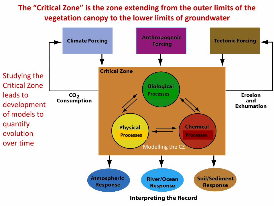
The “Critical Zone” is the zone extending from the outer limits of the vegetation canopy to the lower limits of groundwater

Photo by Andy Pike, (Univ Penn), Luquillo CZO

Studying the Critical Zone leads to development of models to quantify evolution over time

Modelling the CZ

Processes

Processes Processes

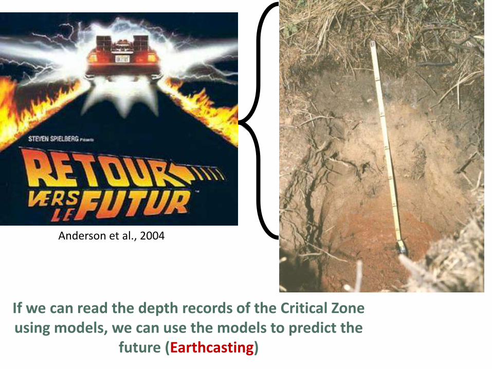
If we can read the depth records of the Critical Zone using models, we can use the models to predict the

future (Earthcasting)

ALL PROCESSES IN THE CRITICAL ZONE

Anderson et al., 2004 USGS circular 1139

Critical Zone Science Mission: • Learn to measure the fluxes

occurring today

• Learn to read the geological record of the cumulative effect of these fluxes over time

• Develop quantitative models of Critical Zone evolution

Critical Zone Science Vision:

By measuring what is happening today and reading what happened yesterday, we will learn to project

what will happen tomorrow

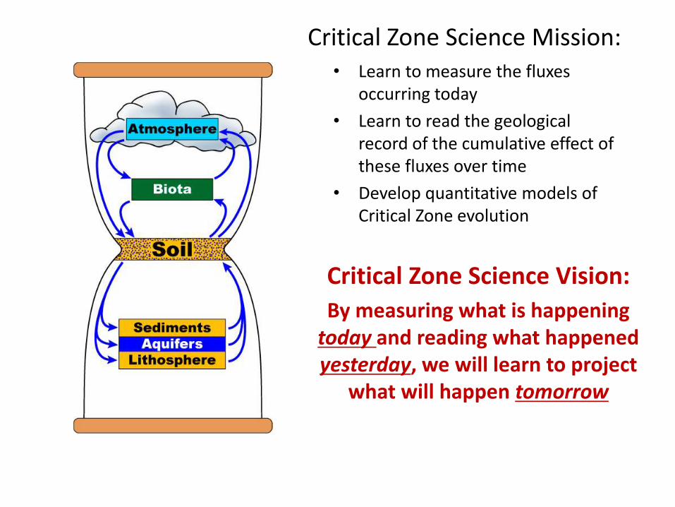
Critical Zone Science Mission: • Learn to measure the fluxes

occurring today

• Learn to read the geological record of the cumulative effect of these fluxes over time

• Develop quantitative models of Critical Zone evolution

Critical Zone Science Vision:

By measuring what is happening today and reading what happened yesterday, we will learn to project

what will happen tomorrow

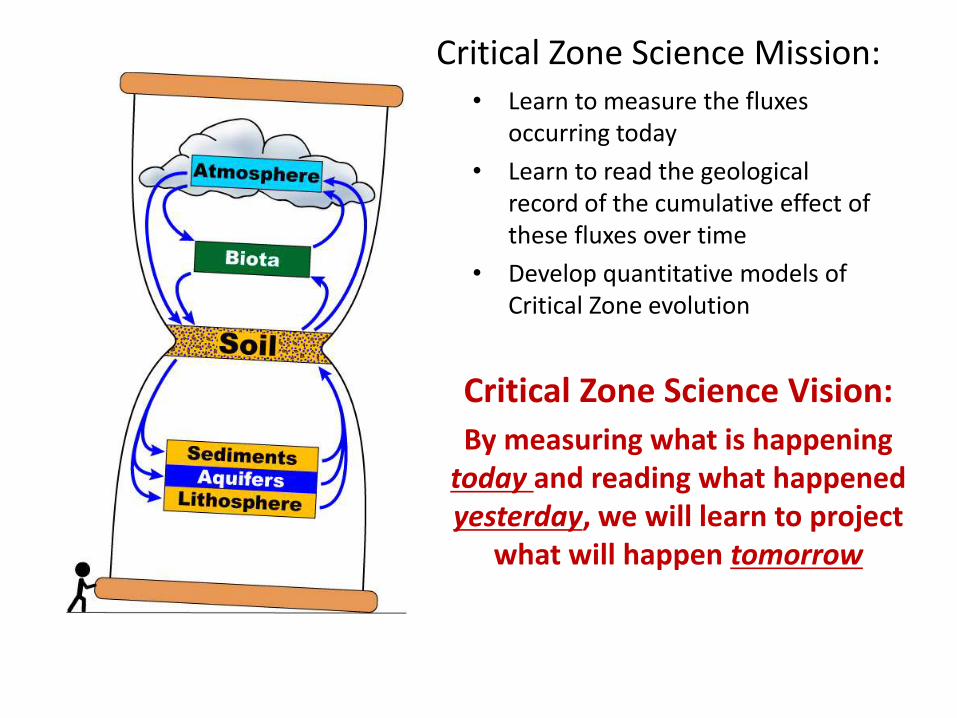
Welcome to the Anthropocene

• “The Earth is a big thing; if you divided it up evenly among its 7 billion inhabitants, they would get almost 1 trillion tonnes each. To think that the workings of so vast an entity could be lastingly changed by a species that has been scampering across its surface for less than 1% of its history seems, on the face of it, absurd. But it is not. Humans have become a force of nature reshaping the planet on a geological scale – but at a far-faster-than-geological speed.” From: The Economist: May 28, 2011

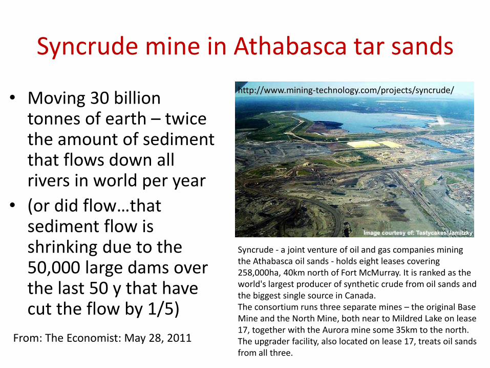
Syncrude mine in Athabasca tar sands

• Moving 30 billion tonnes of earth – twice the amount of sediment that flows down all rivers in world per year

• (or did flow…that sediment flow is shrinking due to the 50,000 large dams over the last 50 y that have cut the flow by 1/5)

From: The Economist: May 28, 2011

Syncrude - a joint venture of oil and gas companies mining the Athabasca oil sands - holds eight leases covering 258,000ha, 40km north of Fort McMurray. It is ranked as the world's largest producer of synthetic crude from oil sands and the biggest single source in Canada. The consortium runs three separate mines – the original Base Mine and the North Mine, both near to Mildred Lake on lease 17, together with the Aurora mine some 35km to the north. The upgrader facility, also located on lease 17, treats oil sands from all three.

http://www.mining-technology.com/projects/syncrude/

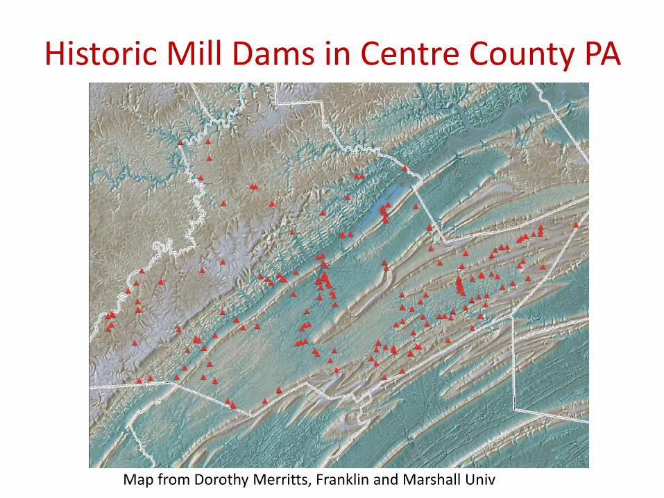
Historic Mill Dams in Centre County PA

Map from Dorothy Merritts, Franklin and Marshall Univ

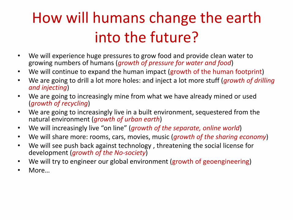
How will humans change the earth into the future?

• We will experience huge pressures to grow food and provide clean water to growing numbers of humans (growth of pressure for water and food)

• We will continue to expand the human impact (growth of the human footprint) • We are going to drill a lot more holes: and inject a lot more stuff (growth of drilling

and injecting) • We are going to increasingly mine from what we have already mined or used

(growth of recycling) • We are going to increasingly live in a built environment, sequestered from the

natural environment (growth of urban earth) • We will increasingly live “on line” (growth of the separate, online world) • We will share more: rooms, cars, movies, music (growth of the sharing economy) • We will see push back against technology , threatening the social license for

development (growth of the No-society) • We will try to engineer our global environment (growth of geoengineering) • More…

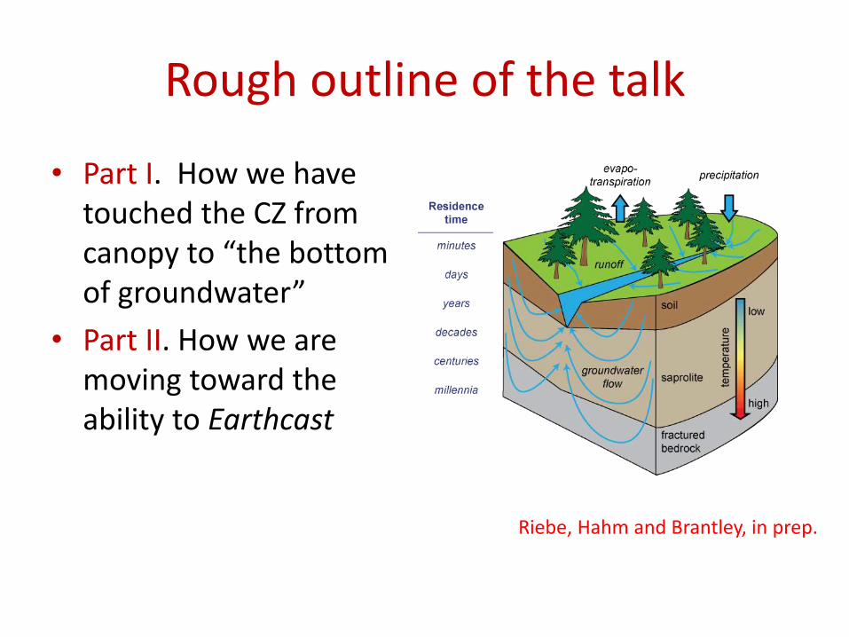
• Part I. How we have touched the CZ from canopy to “the bottom of groundwater”

• Part II. How we are moving toward the ability to Earthcast

Riebe, Hahm and Brantley, in prep.

Rough outline of the talk

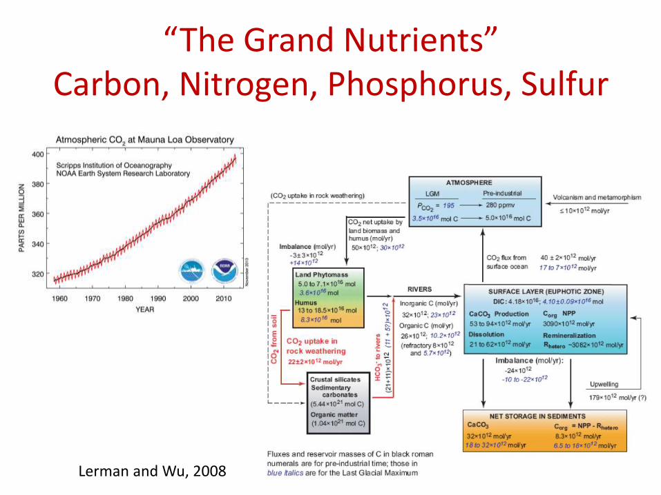
“The Grand Nutrients” Carbon, Nitrogen, Phosphorus, Sulfur

Lerman and Wu, 2008

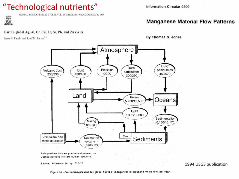
1994 USGS publication

“Technological nutrients”

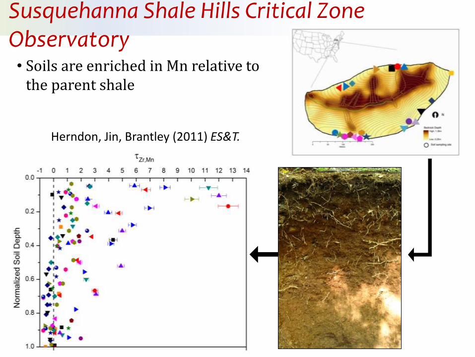
Herndon, Jin, Brantley (2011) ES&T.

Susquehanna Shale Hills Observatory (SSHO)

• Soils are enriched in Mn relative to the parent shale

Susquehanna Shale Hills Critical Zone Observatory

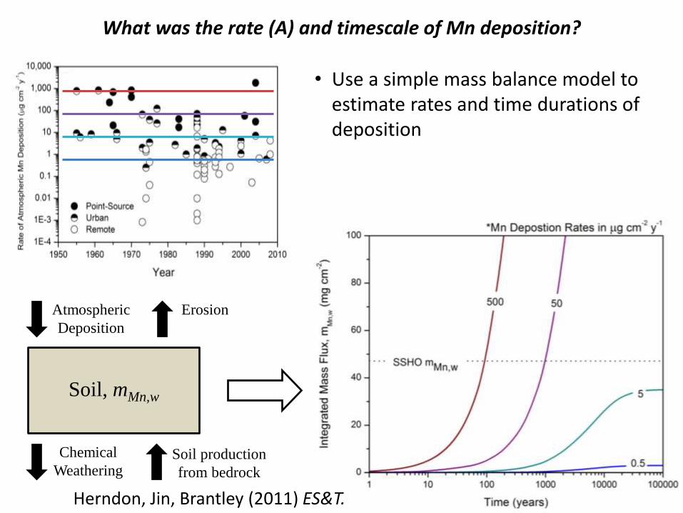
• Use a simple mass balance model to estimate rates and time durations of deposition

Soil, mMn,w

Atmospheric

Deposition

Chemical

Weathering

Soil production

from bedrock

Erosion

What was the rate (A) and timescale of Mn deposition?


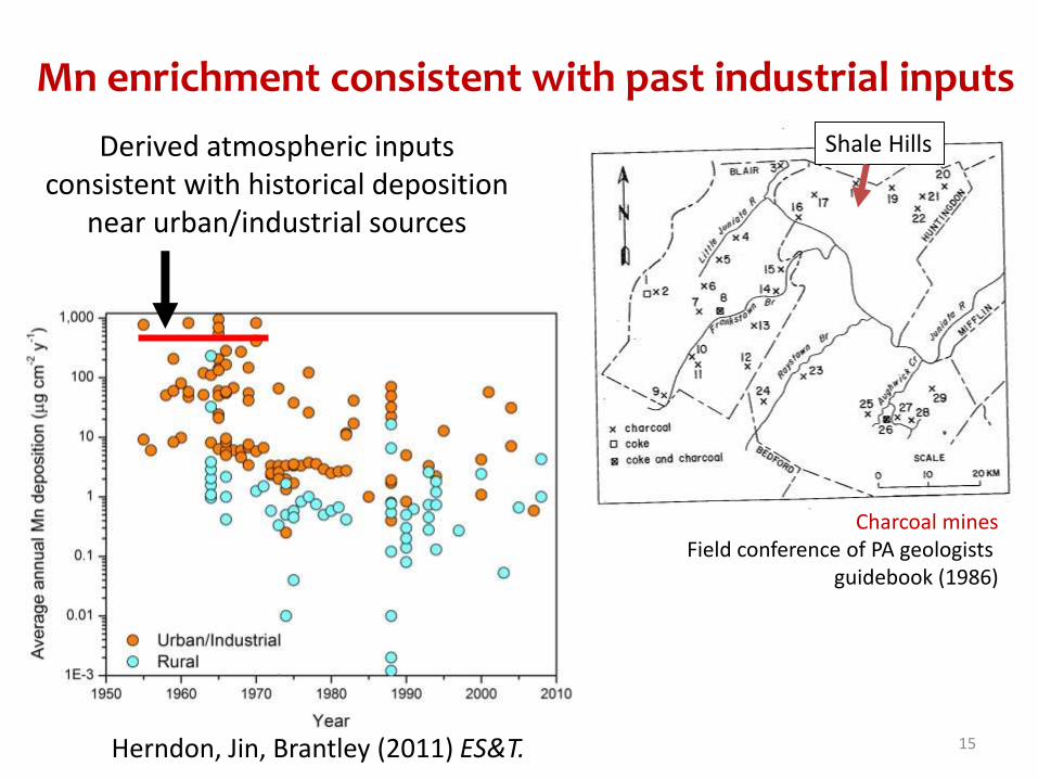
Mn enrichment consistent with past industrial inputs

Derived atmospheric inputs consistent with historical deposition

near urban/industrial sources

15

Charcoal mines Field conference of PA geologists

guidebook (1986)

Shale Hills


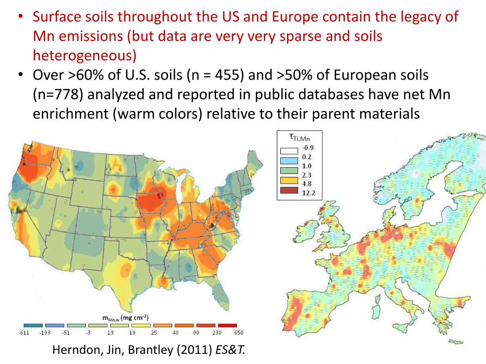
• Surface soils throughout the US and Europe contain the legacy of Mn emissions (but data are very very sparse and soils heterogeneous)

• Over >60% of U.S. soils (n = 455) and >50% of European soils (n=778) analyzed and reported in public databases have net Mn enrichment (warm colors) relative to their parent materials


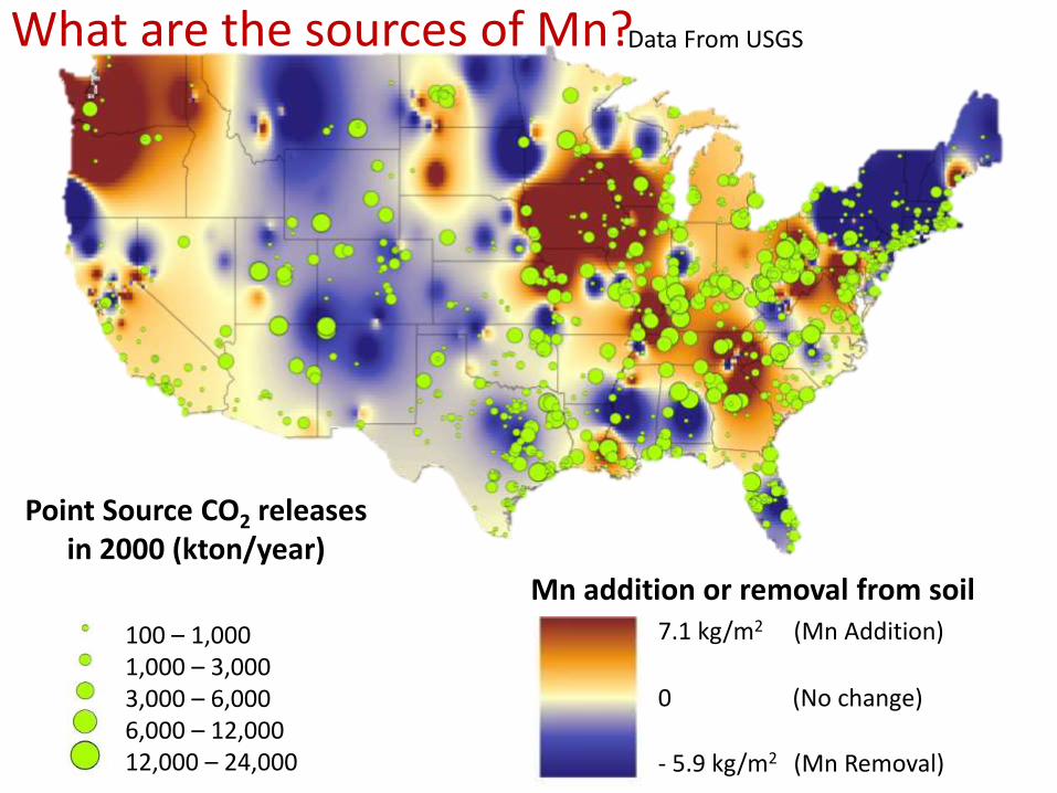
100 – 1,000 1,000 – 3,000 3,000 – 6,000 6,000 – 12,000 12,000 – 24,000

Point Source CO2 releases in 2000 (kton/year)

Mn addition or removal from soil 7.1 kg/m2 (Mn Addition)

- 5.9 kg/m2 (Mn Removal)

0 (No change)

Data From USGS What are the sources of Mn?

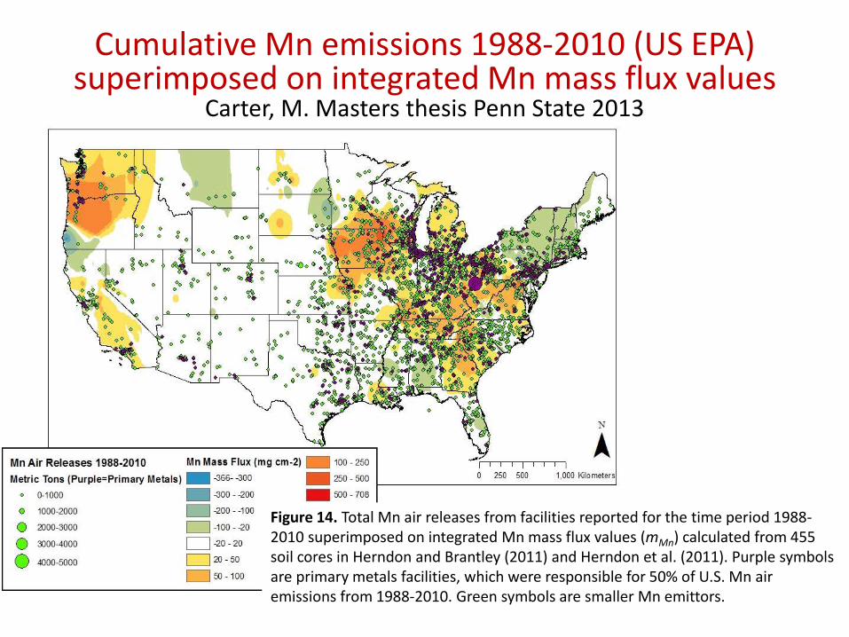
Cumulative Mn emissions 1988-2010 (US EPA) superimposed on integrated Mn mass flux values

Carter, M. Masters thesis Penn State 2013

Figure 14. Total Mn air releases from facilities reported for the time period 1988-2010 superimposed on integrated Mn mass flux values (mMn) calculated from 455 soil cores in Herndon and Brantley (2011) and Herndon et al. (2011). Purple symbols are primary metals facilities, which were responsible for 50% of U.S. Mn air emissions from 1988-2010. Green symbols are smaller Mn emittors.

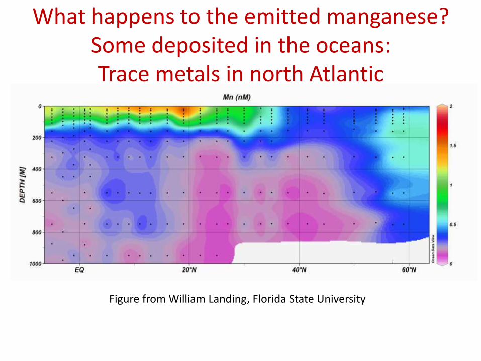
What happens to the emitted manganese? Some deposited in the oceans: Trace metals in north Atlantic

Figure from William Landing, Florida State University

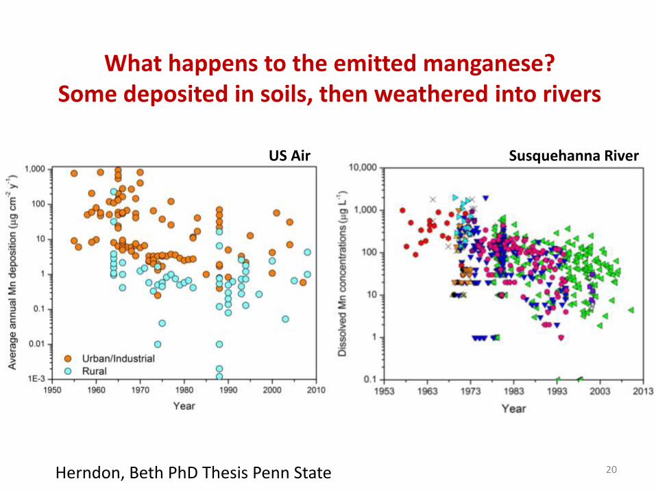
What happens to the emitted manganese? Some deposited in soils, then weathered into rivers

20

US Air Susquehanna River

Herndon, Beth PhD Thesis Penn State

21

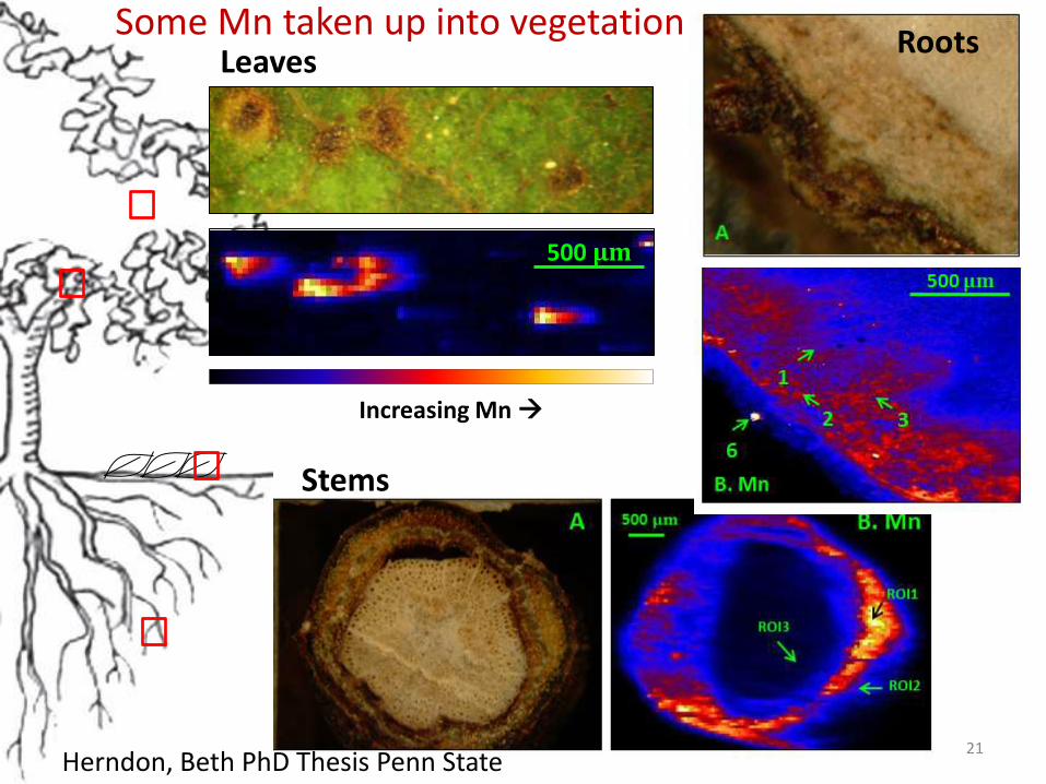
500 µm

Increasing Mn

Leaves

Stems

Roots

Herndon, Beth PhD Thesis Penn State

Some Mn taken up into vegetation

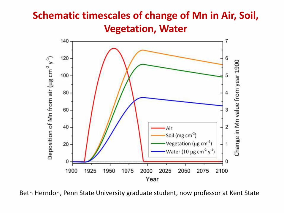
Schematic timescales of change of Mn in Air, Soil, Vegetation, Water

Beth Herndon, Penn State University graduate student, now professor at Kent State

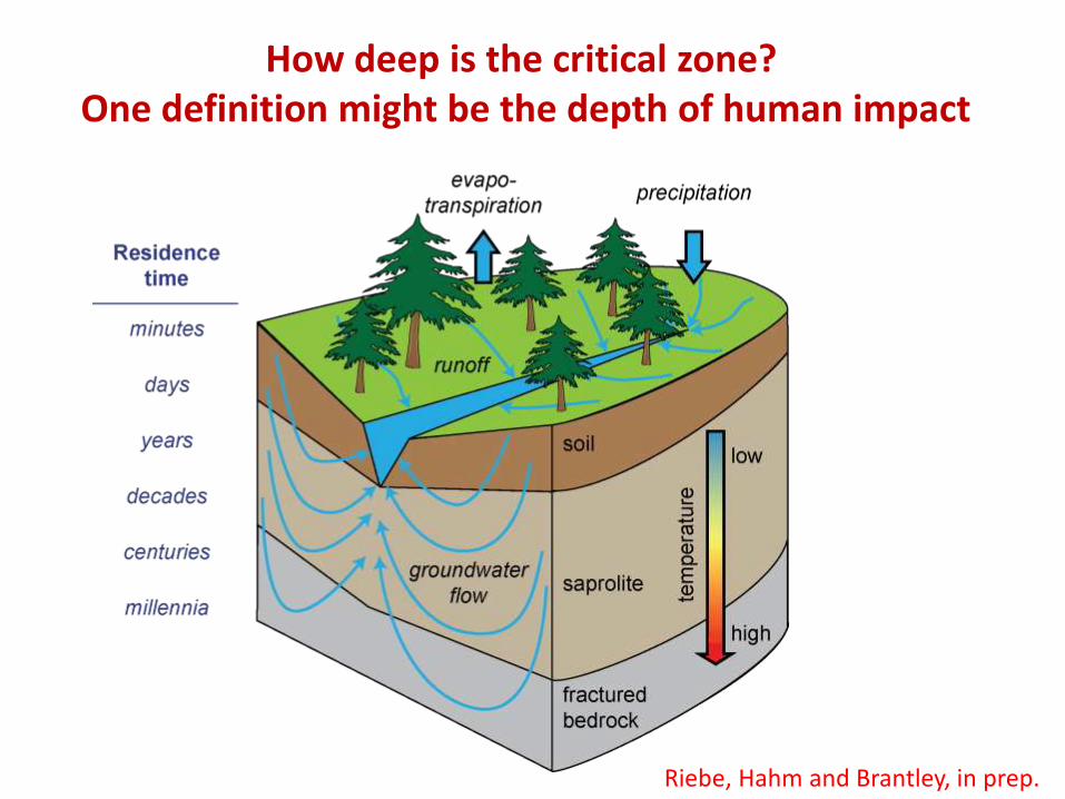
How deep is the critical zone? One definition might be the depth of human impact

Riebe, Hahm and Brantley, in prep.

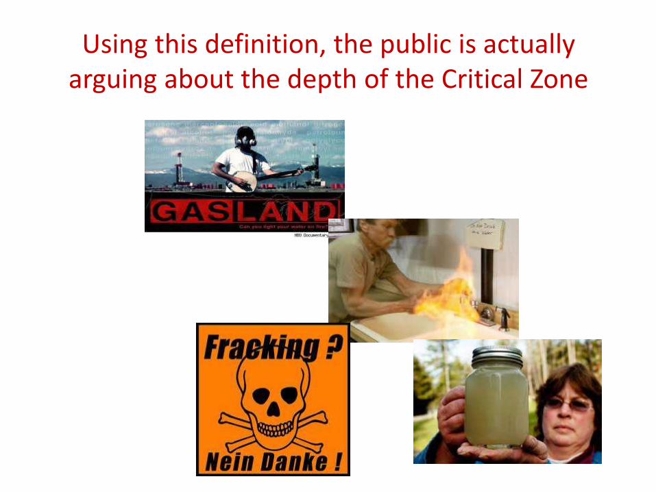
Using this definition, the public is actually arguing about the depth of the Critical Zone

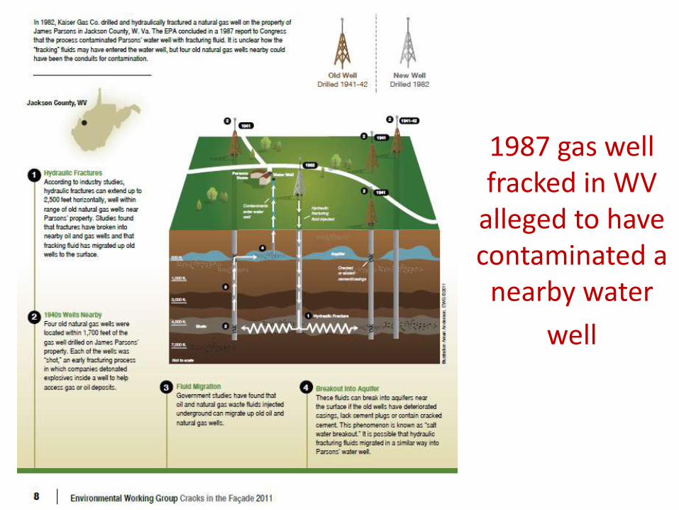
1987 gas well fracked in WV

alleged to have contaminated a

nearby water

well

From EPA report

• In 1982, Kaiser Gas Co. drilled a gas well on the property of Mr. James Parsons. The well was fractured using a typical fracturing fluid or gel. The residual fracturing fluid migrated into Mr. Parson’s water well (which was drilled to a depth of 416 feet), according to an analysis by the West Virginia Environmental Health Services Lab of well water samples taken from the property. Dark and light gelatinous material (fracturing fluid) was found, along with white fibers. The gas well is located less than 1000 feet from the water well. The chief of the laboratory advised that the water well was contaminated and unfit for domestic use, and that an alternative source of domestic water had to be found. Analysis showed the water to contain high levels of fluoride, sodium, iron, and manganese. The water, according to DNR officials, had a hydrocarbon odor, indicating the presence of gas.

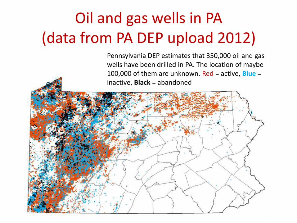
Oil and gas wells in PA (data from PA DEP upload 2012)

Pennsylvania DEP estimates that 350,000 oil and gas wells have been drilled in PA. The location of maybe 100,000 of them are unknown. Red = active, Blue = inactive, Black = abandoned

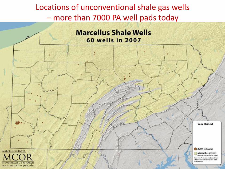
Locations of unconventional shale gas wells – more than 7000 PA well pads today

THE NSF-FUNDED SHALE NETWORK

The ShaleNetwork is creating a central and accessible repository for geochemistry and hydrology data collected by watershed groups, government agencies, industry stakeholders, and universities working together to document natural variability and potential environmental impacts of shale gas extraction activities.

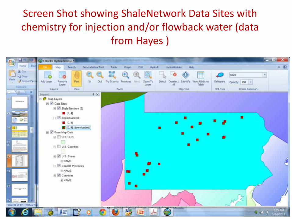
Screen Shot showing ShaleNetwork Data Sites with chemistry for injection and/or flowback water (data

from Hayes )

0

500

1000

1500

2000

2500

0 10 20 30 40 50 60 70 80 90 100

Co

nce

ntr

atio

n, p

pb

Days after hydrofracturing

Benzene

A

B

C

D

E

F

G

H

I

J

K

L

M

N

O

P

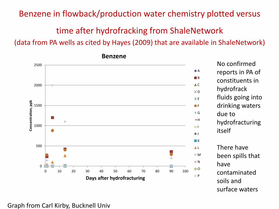
Graph from Carl Kirby, Bucknell Univ

No confirmed reports in PA of constituents in hydrofrack fluids going into drinking waters due to hydrofracturing itself There have been spills that have contaminated soils and surface waters

Benzene in flowback/production water chemistry plotted versus

time after hydrofracking from ShaleNetwork (data from PA wells as cited by Hayes (2009) that are available in ShaleNetwork)

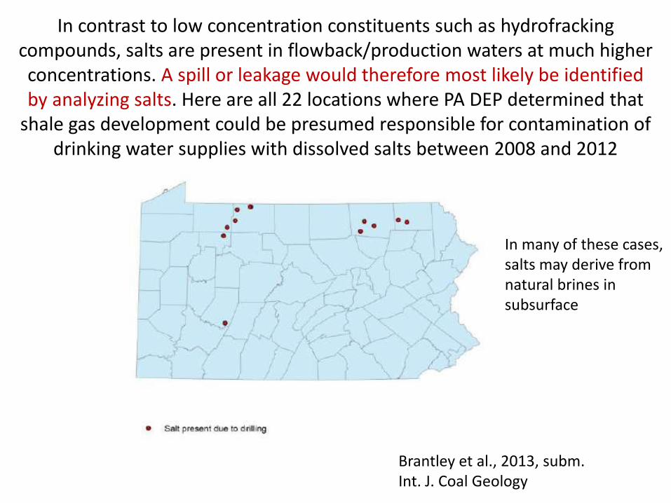
In contrast to low concentration constituents such as hydrofracking compounds, salts are present in flowback/production waters at much higher concentrations. A spill or leakage would therefore most likely be identified by analyzing salts. Here are all 22 locations where PA DEP determined that

shale gas development could be presumed responsible for contamination of drinking water supplies with dissolved salts between 2008 and 2012

Brantley et al., 2013, subm. Int. J. Coal Geology

In many of these cases, salts may derive from natural brines in subsurface

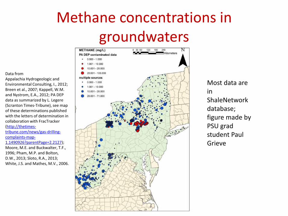
Methane concentrations in groundwaters

Most data are in ShaleNetwork database; figure made by PSU grad student Paul Grieve

Data from Appalachia Hydrogeologic and Environmental Consulting, I., 2012; Breen et al., 2007; Kappell, W.M. and Nystrom, E.A., 2012; PA DEP data as summarized by L. Legere (Scranton Times-Tribune), see map of these determinations published with the letters of determination in collaboration with FracTracker (http://thetimes-tribune.com/news/gas-drilling-complaints-map-1.1490926?parentPage=2.2127); Moore, M.E. and Buckwalter, T.F., 1996; Pham, M.P. and Bolton, D.W., 2013; Sloto, R.A., 2013; White, J.S. and Mathes, M.V., 2006.

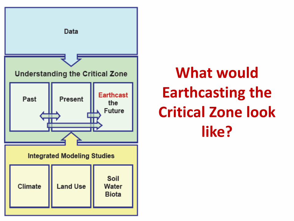
http://thetimes-tribune.com/news/gas-drilling-complaints-map-1.1490926?parentPage=2.2127











What would Earthcasting the Critical Zone look

like?

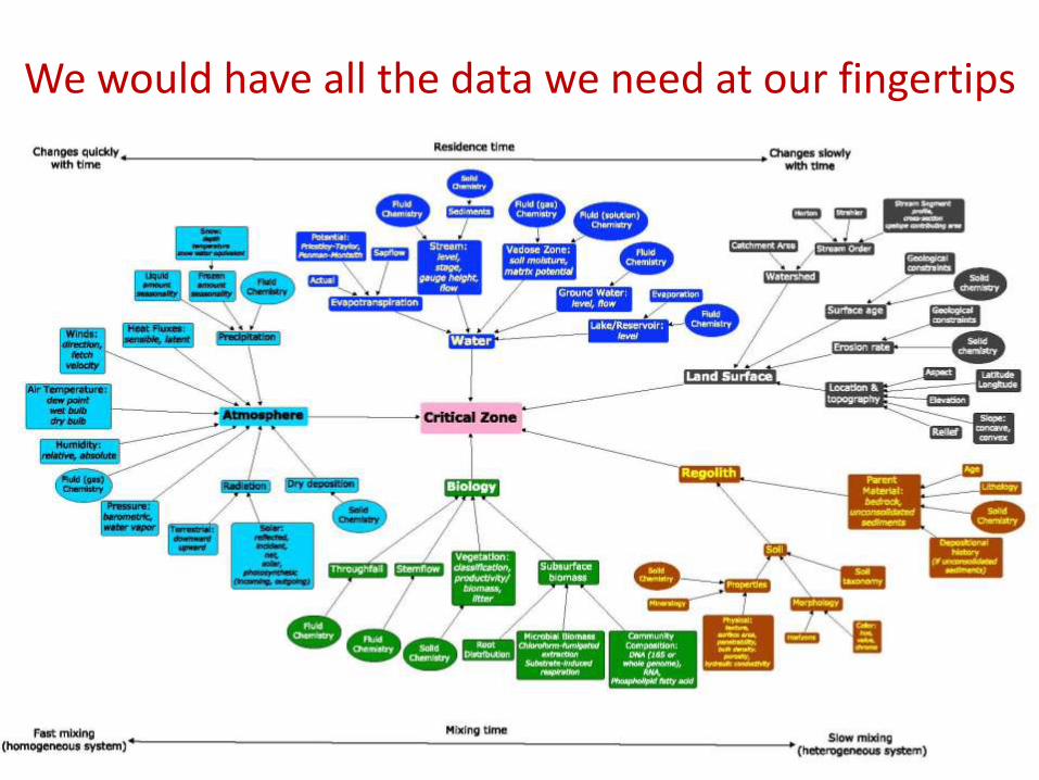
We would have all the data we need at our fingertips

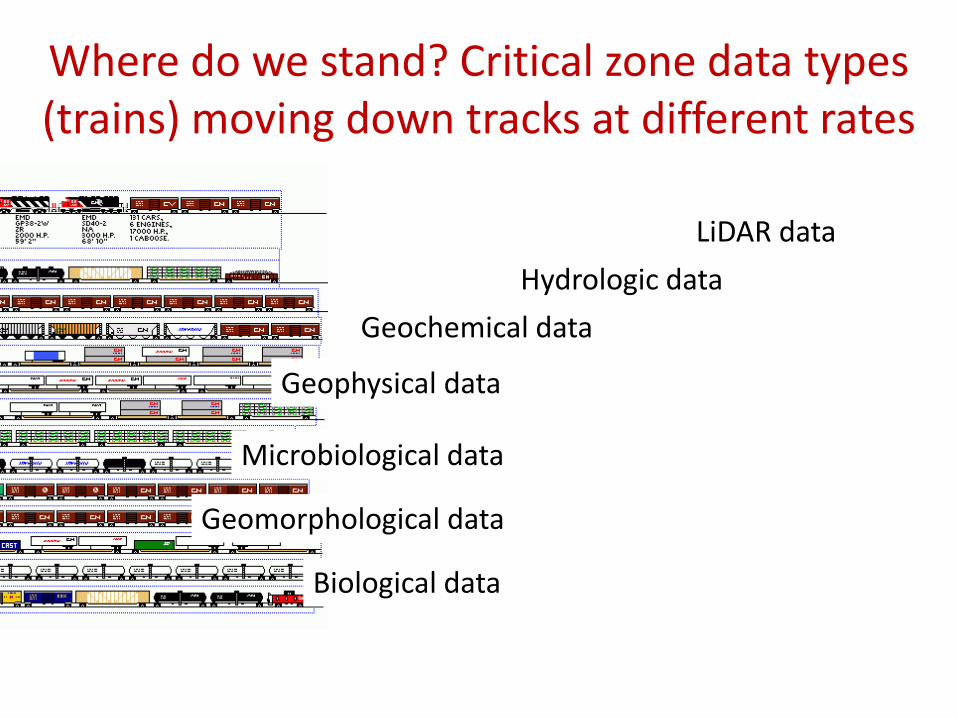
Where do we stand? Critical zone data types (trains) moving down tracks at different rates

Geochemical data

Hydrologic data

Geophysical data

Microbiological data

Geomorphological data

Biological data

LiDAR data

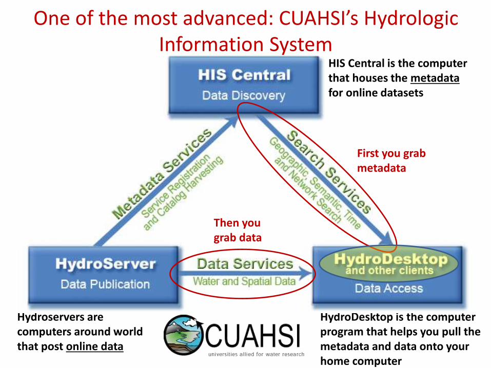
Hydroservers are computers around world that post online data

HydroDesktop is the computer program that helps you pull the metadata and data onto your home computer

One of the most advanced: CUAHSI’s Hydrologic Information System

HIS Central is the computer that houses the metadata for online datasets

First you grab metadata

Then you grab data

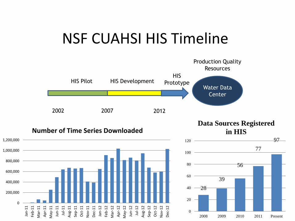
2002 2007 2012

Water Data

Center

HIS Pilot HIS Development HIS

Prototype

NSF CUAHSI HIS Timeline

Production Quality

Resources

0

200,000

400,000

600,000

800,000

1,000,000

1,200,000

Jan

-11

Feb

-11

Mar

-11

Ap

r-1

1

May

-11

Jun

-11

Jul-

11

Au

g-1

1

Sep

-11

Oct

-11

No

v-1

1

De

c-1

1

Jan

-12

Feb

-12

Mar

-12

Ap

r-1

2

May

-12

Jun

-12

Jul-

12

Au

g-1

2

Sep

-12

Oct

-12

No

v-1

2

De

c-1

2

Number of Time Series Downloaded

28

39

56

77

97

0

20

40

60

80

100

120

2008 2009 2010 2011 Present

Data Sources Registered

in HIS

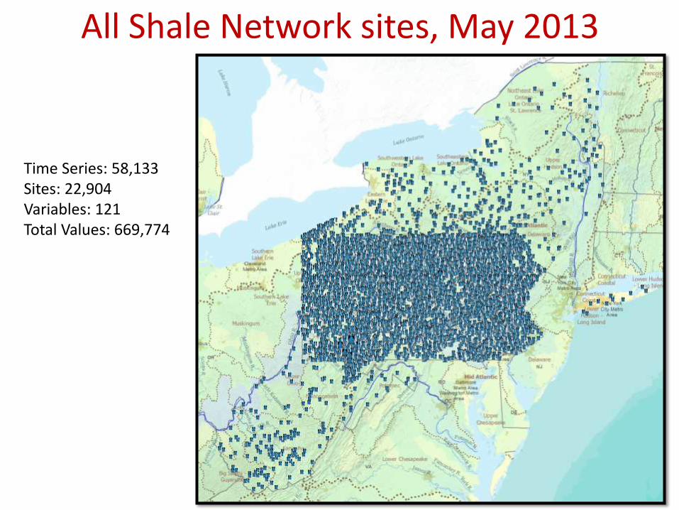
All Shale Network sites, May 2013

Time Series: 58,133 Sites: 22,904 Variables: 121 Total Values: 669,774

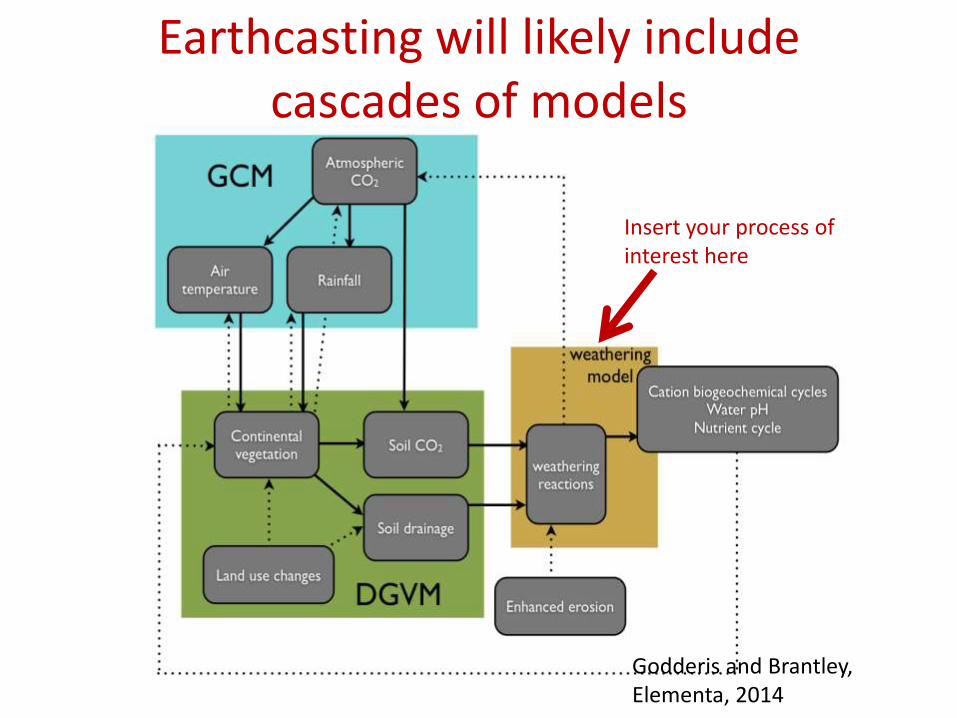
Earthcasting will likely include cascades of models

Insert your process of interest here

Godderis and Brantley, Elementa, 2014

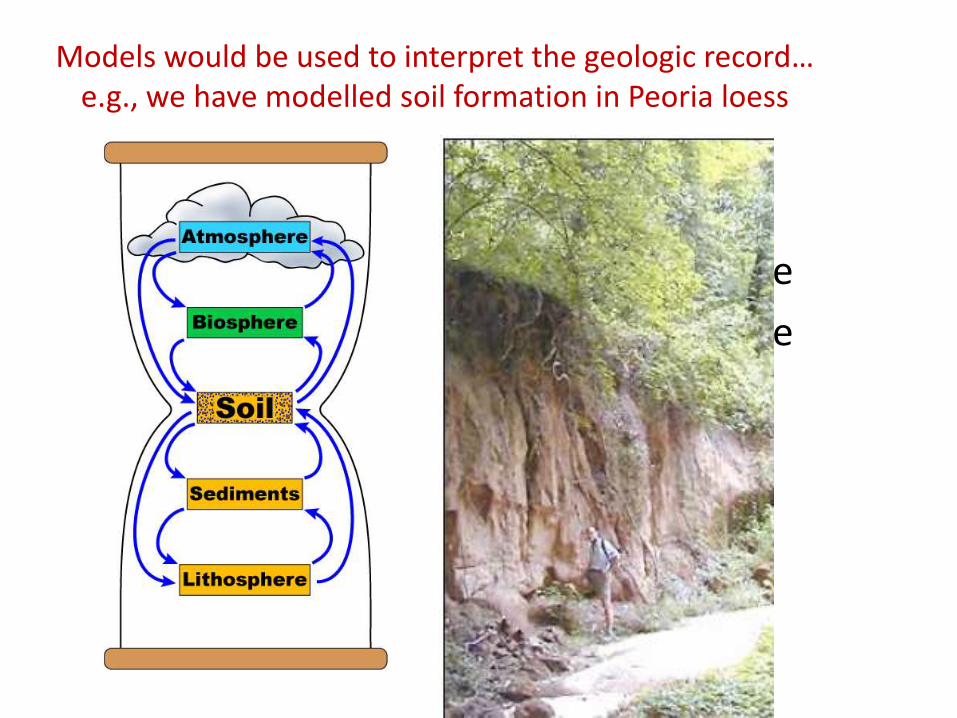
Models would be used to interpret the geologic record… e.g., we have modelled soil formation in Peoria loess

• 102 year timescale

• 104 year timescale

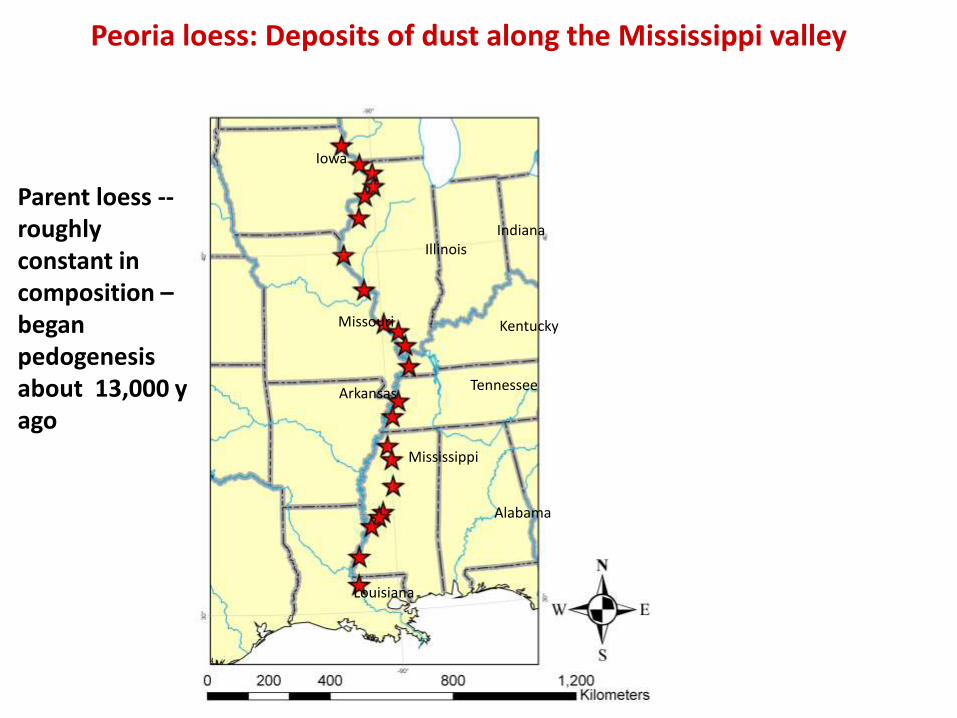
Peoria loess: Deposits of dust along the Mississippi valley

Iowa

Missouri

Arkansas

Louisiana

Illinois Indiana

Kentucky

Tennessee

Mississippi

Alabama

Parent loess -- roughly constant in composition – began pedogenesis about 13,000 y ago

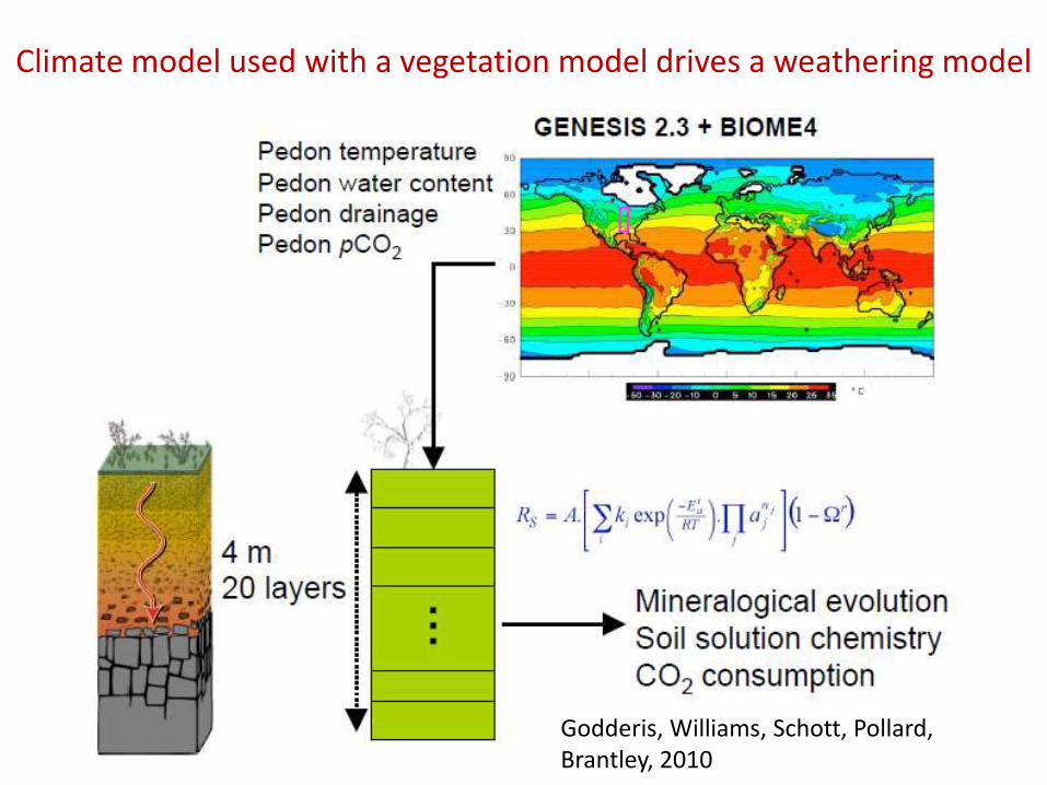
Climate model used with a vegetation model drives a weathering model

Godderis, Williams, Schott, Pollard, Brantley, 2010

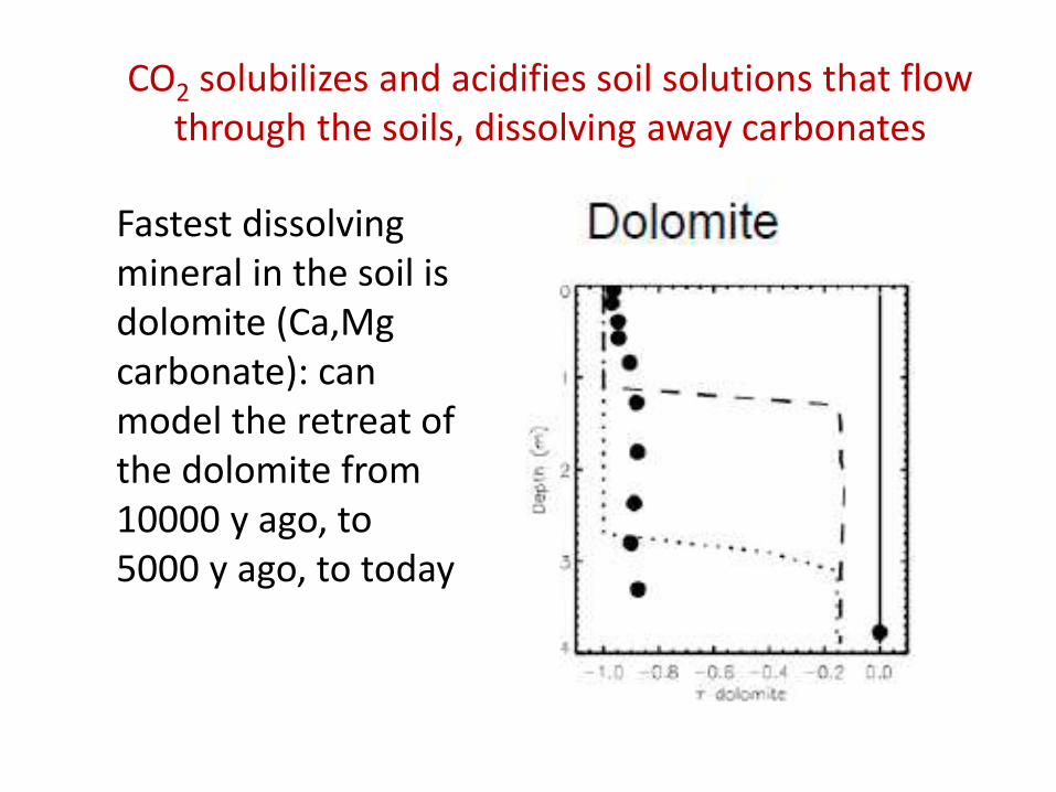
Fastest dissolving mineral in the soil is dolomite (Ca,Mg carbonate): can model the retreat of the dolomite from 10000 y ago, to 5000 y ago, to today

CO2 solubilizes and acidifies soil solutions that flow through the soils, dissolving away carbonates

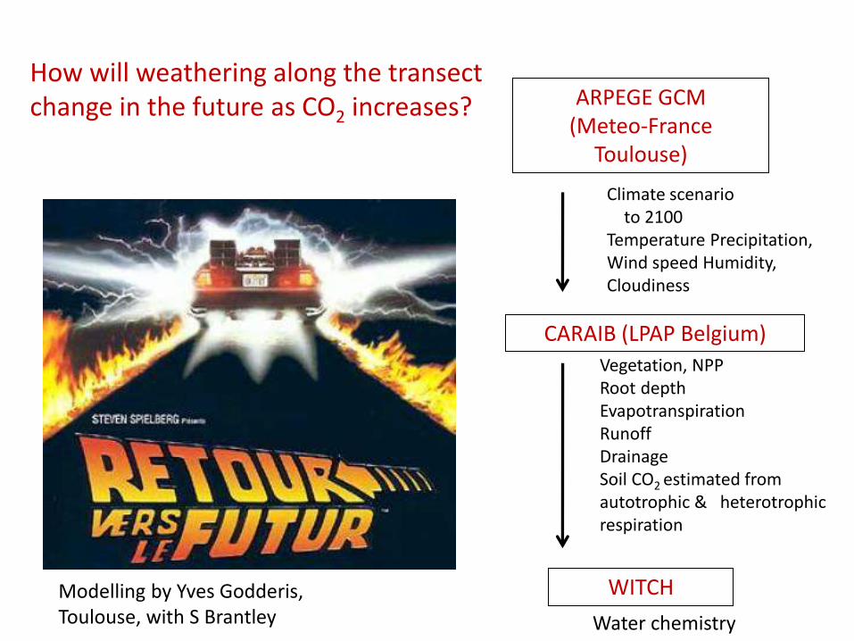
ARPEGE GCM (Meteo-France

Toulouse)

CARAIB (LPAP Belgium)

WITCH

Climate scenario to 2100 Temperature Precipitation, Wind speed Humidity, Cloudiness

Vegetation, NPP Root depth Evapotranspiration Runoff Drainage Soil CO2 estimated from autotrophic & heterotrophic respiration

Water chemistry

Modelling by Yves Godderis, Toulouse, with S Brantley

How will weathering along the transect change in the future as CO2 increases?

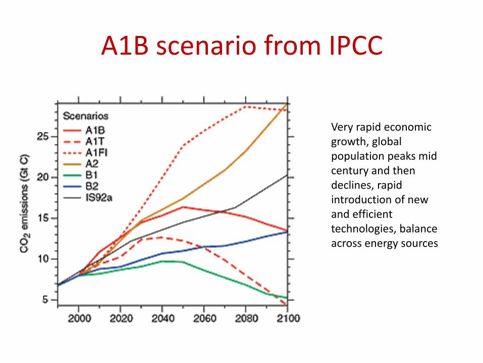
A1B scenario from IPCC

Very rapid economic growth, global population peaks mid century and then declines, rapid introduction of new and efficient technologies, balance across energy sources

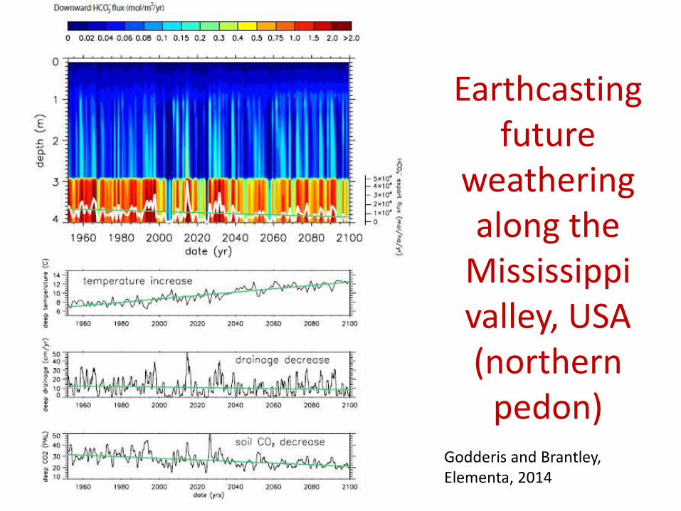
Earthcasting future

weathering along the

Mississippi valley, USA (northern

pedon) Godderis and Brantley, Elementa, 2014

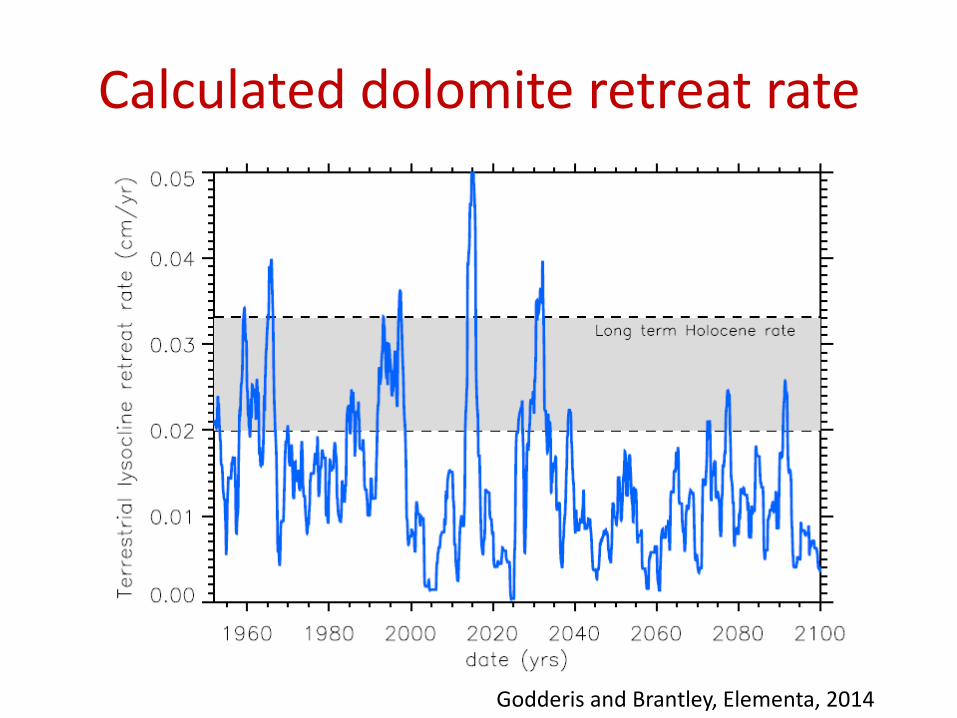
Calculated dolomite retreat rate

Godderis and Brantley, Elementa, 2014

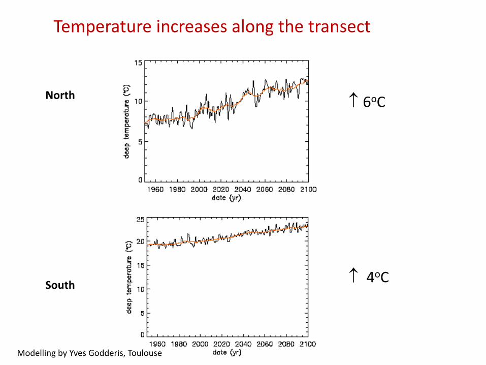
Temperature increases along the transect

North South

6oC 4oC

Modelling by Yves Godderis, Toulouse

North South

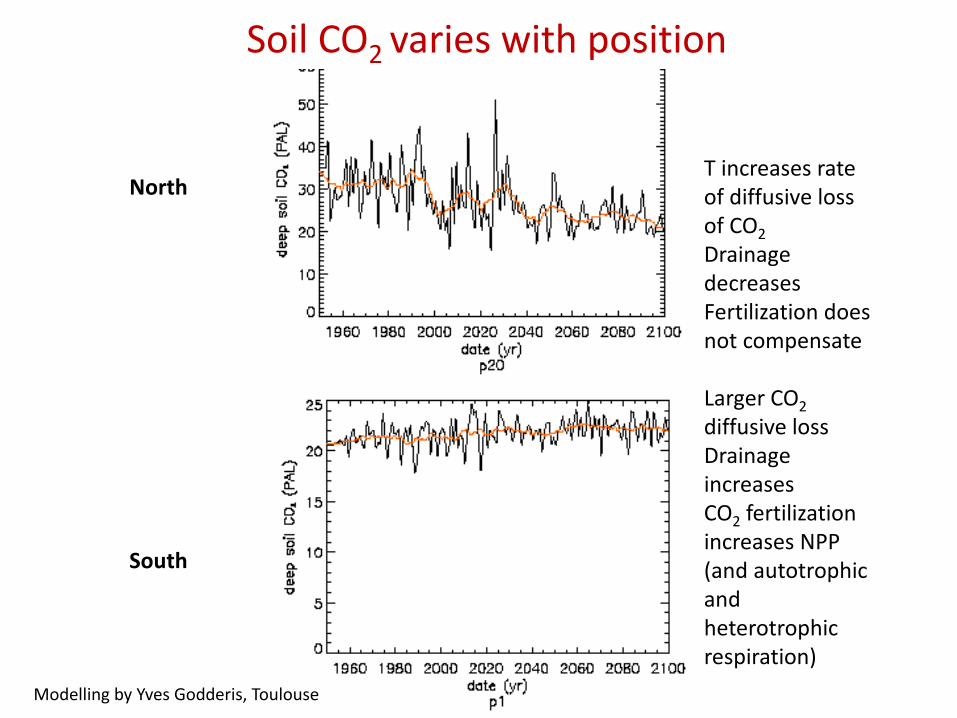
T increases rate of diffusive loss of CO2

Drainage decreases Fertilization does not compensate Larger CO2 diffusive loss Drainage increases CO2 fertilization increases NPP (and autotrophic and heterotrophic respiration)


Soil CO2 varies with position

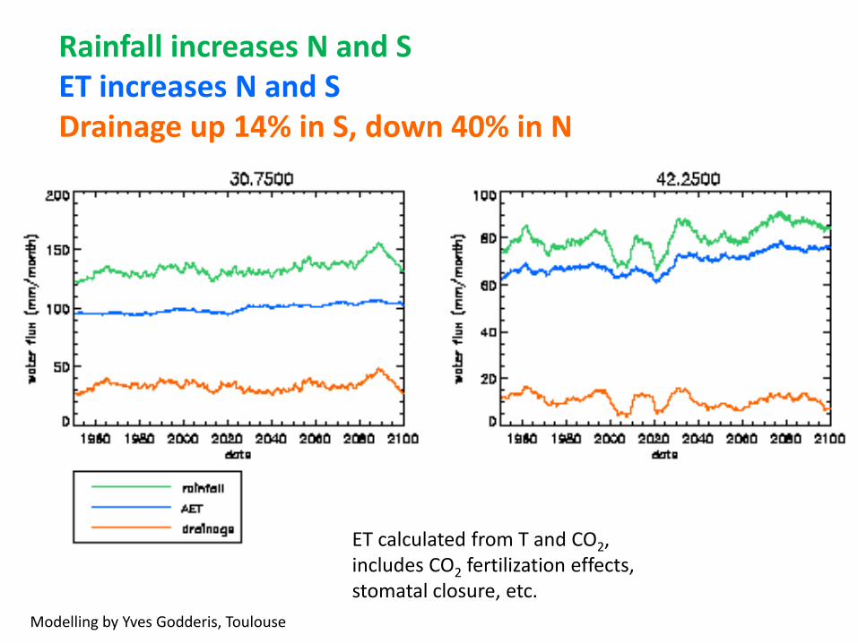
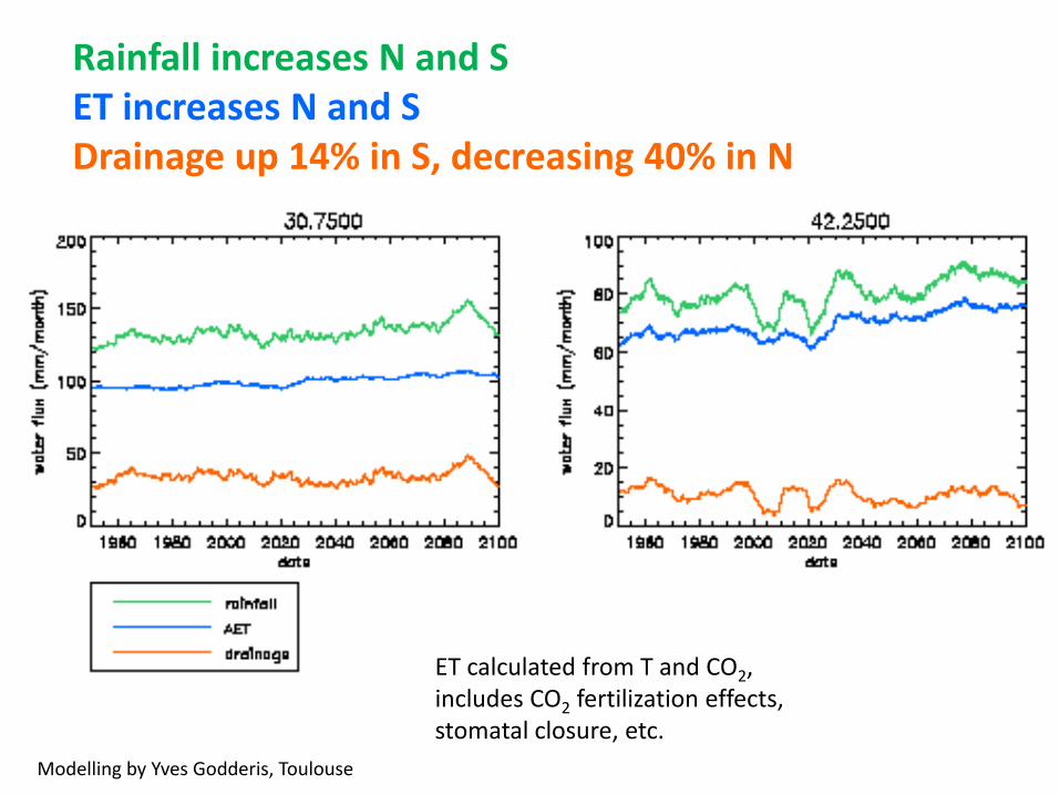
Rainfall increases N and S ET increases N and S Drainage up 14% in S, down 40% in N

ET calculated from T and CO2, includes CO2 fertilization effects, stomatal closure, etc.


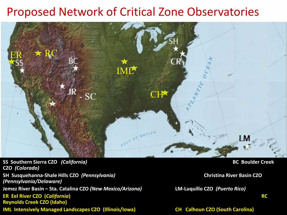
Proposed Network of Critical Zone Observatories

ER RC

IML

CH - SC

SS Southern Sierra CZO (California) BC Boulder Creek CZO (Colorado)

SH Susquehanna-Shale Hills CZO (Pennsylvania) Christina River Basin CZO (Pennsylvania/Delaware)

Jemez River Basin – Sta. Catalina CZO (New Mexico/Arizona) LM-Luquillo CZO (Puerto Rico)

ER Eel River CZO (California) RC Reynolds Creek CZO (Idaho)

IML Intensively Managed Landscapes CZO (Illinois/Iowa) CH Calhoun CZO (South Carolina)

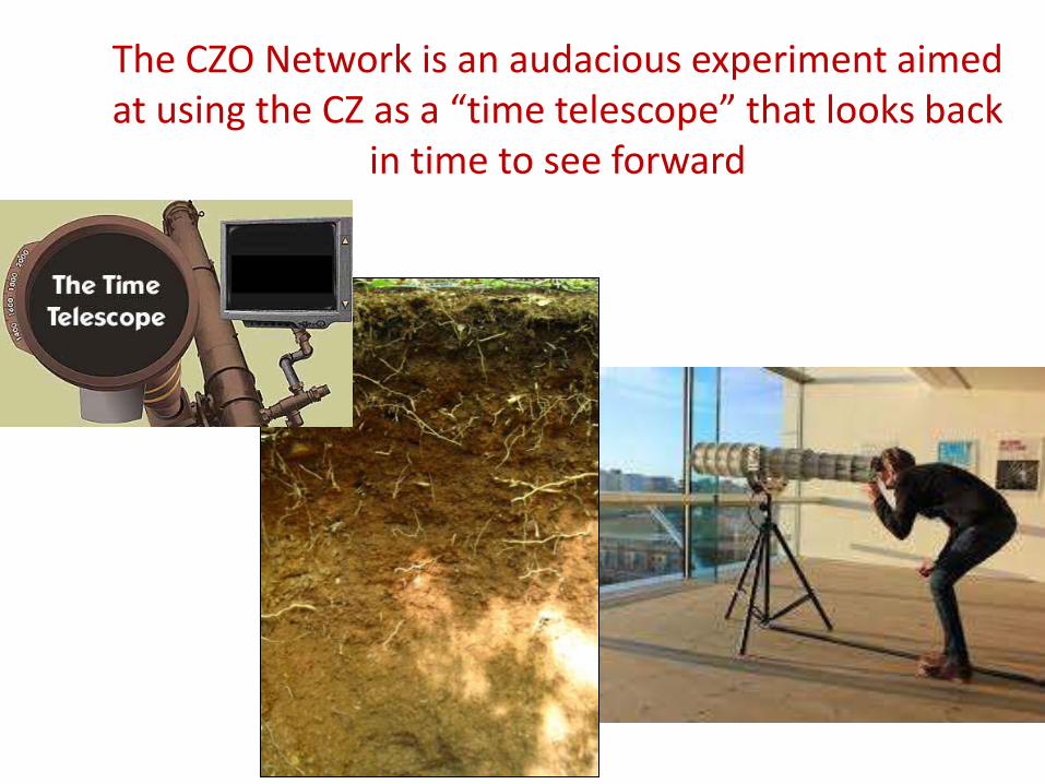
The CZO Network is an audacious experiment aimed at using the CZ as a “time telescope” that looks back

in time to see forward

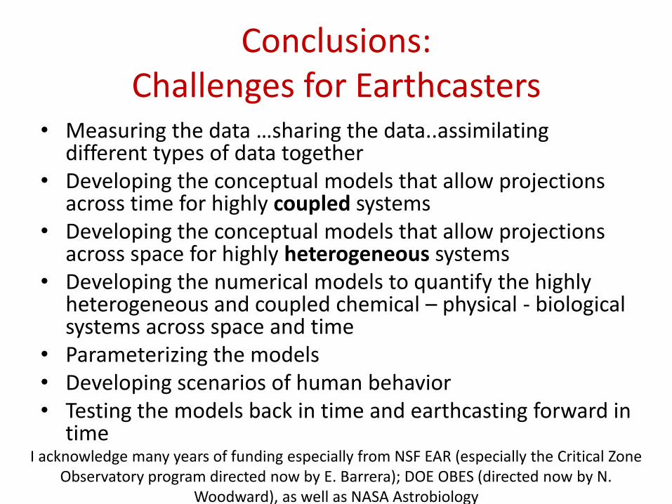
Conclusions: Challenges for Earthcasters

• Measuring the data …sharing the data..assimilating different types of data together

• Developing the conceptual models that allow projections across time for highly coupled systems

• Developing the conceptual models that allow projections across space for highly heterogeneous systems

• Developing the numerical models to quantify the highly heterogeneous and coupled chemical – physical - biological systems across space and time

• Parameterizing the models • Developing scenarios of human behavior • Testing the models back in time and earthcasting forward in

time I acknowledge many years of funding especially from NSF EAR (especially the Critical Zone

Observatory program directed now by E. Barrera); DOE OBES (directed now by N. Woodward), as well as NASA Astrobiology

Coming soon on cable… the Earth Channel?

Landslide occurs

Next years flooding from next year’s hurricane

The Earth Channel

data show enhanced erosion and weathering across southeastern Asia

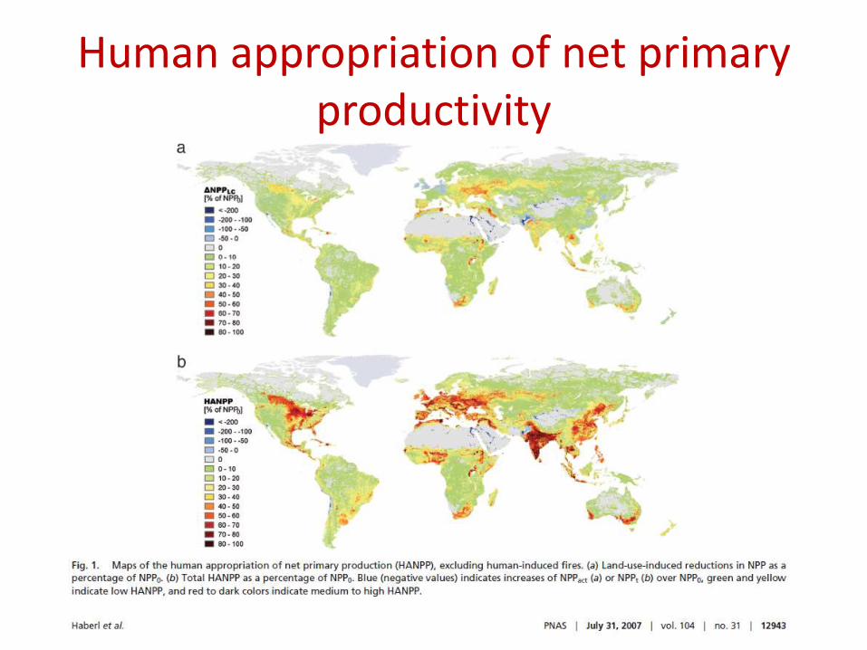
Human appropriation of net primary productivity

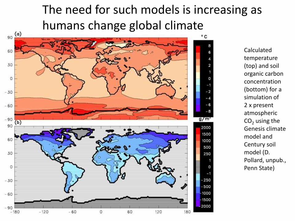
Calculated temperature (top) and soil organic carbon concentration (bottom) for a simulation of 2 x present atmospheric CO2 using the Genesis climate model and Century soil model (D. Pollard, unpub., Penn State)

The need for such models is increasing as humans change global climate

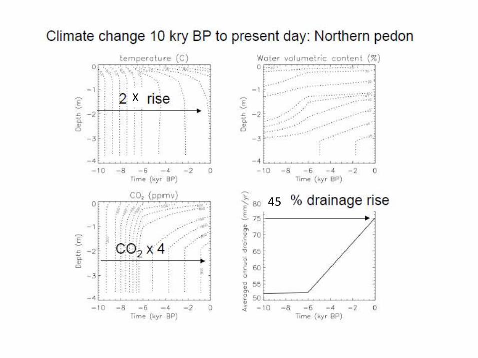
X

45

Temperature increases along the transect

North South

6oC 4oC


Rainfall increases N and S ET increases N and S Drainage up 14% in S, decreasing 40% in N

ET calculated from T and CO2, includes CO2 fertilization effects, stomatal closure, etc.


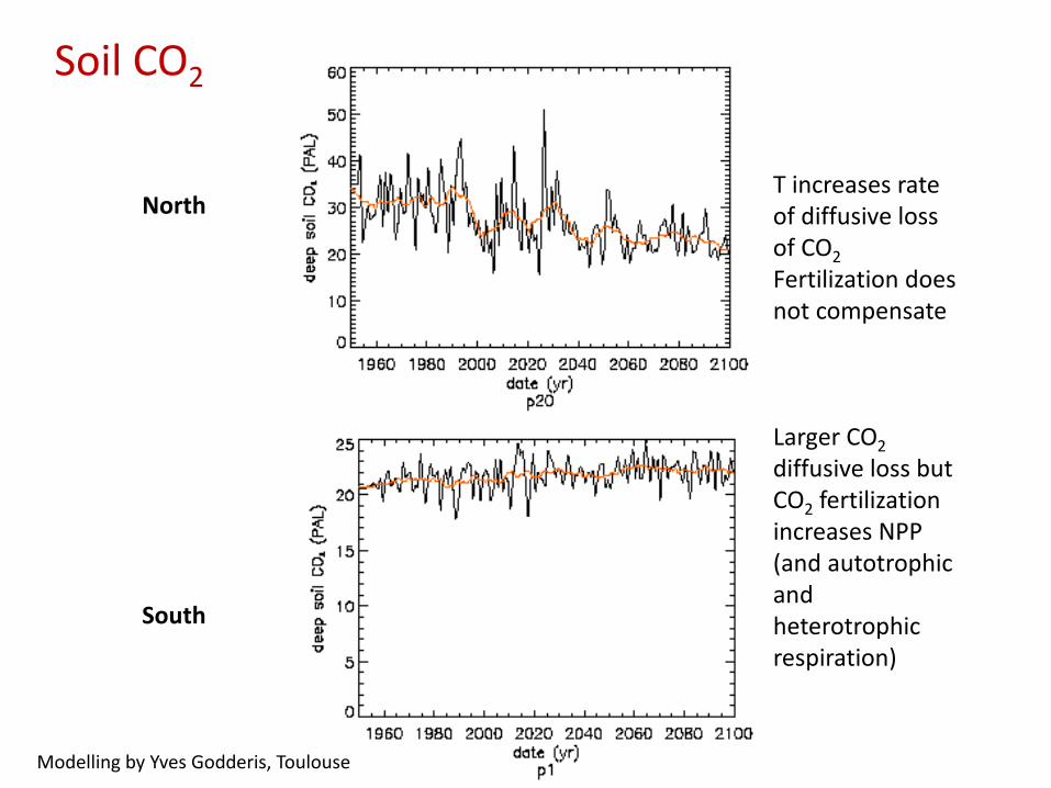
Soil CO2

North South

T increases rate of diffusive loss of CO2

Fertilization does not compensate Larger CO2 diffusive loss but CO2 fertilization increases NPP (and autotrophic and heterotrophic respiration)


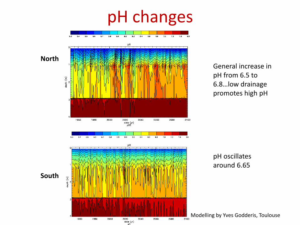
pH changes

North South

General increase in pH from 6.5 to 6.8…low drainage promotes high pH pH oscillates around 6.65


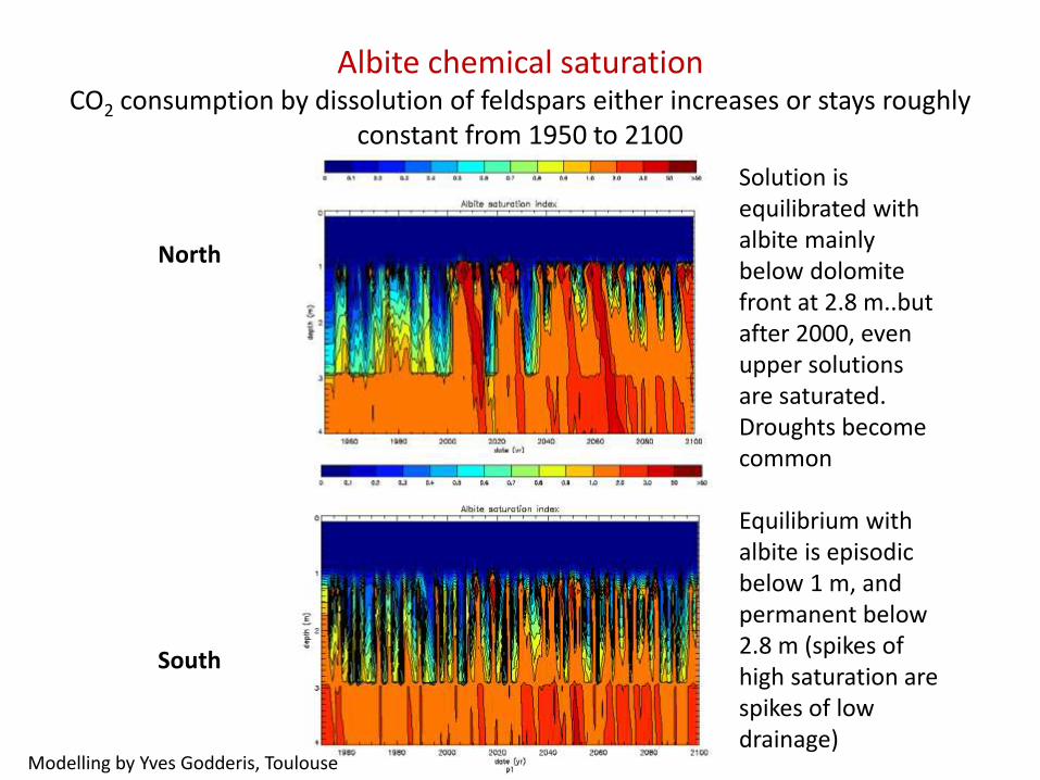
Albite chemical saturation CO2 consumption by dissolution of feldspars either increases or stays roughly

constant from 1950 to 2100

North South

Solution is equilibrated with albite mainly below dolomite front at 2.8 m..but after 2000, even upper solutions are saturated. Droughts become common Equilibrium with albite is episodic below 1 m, and permanent below 2.8 m (spikes of high saturation are spikes of low drainage)


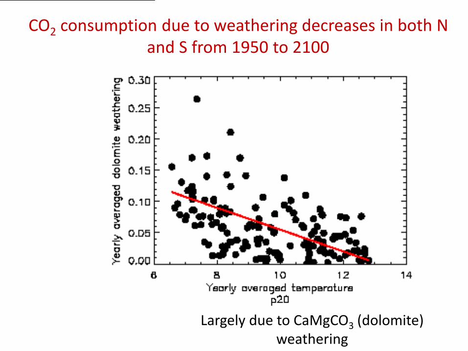
Largely due to CaMgCO3 (dolomite) weathering

CO2 consumption due to weathering decreases in both N and S from 1950 to 2100

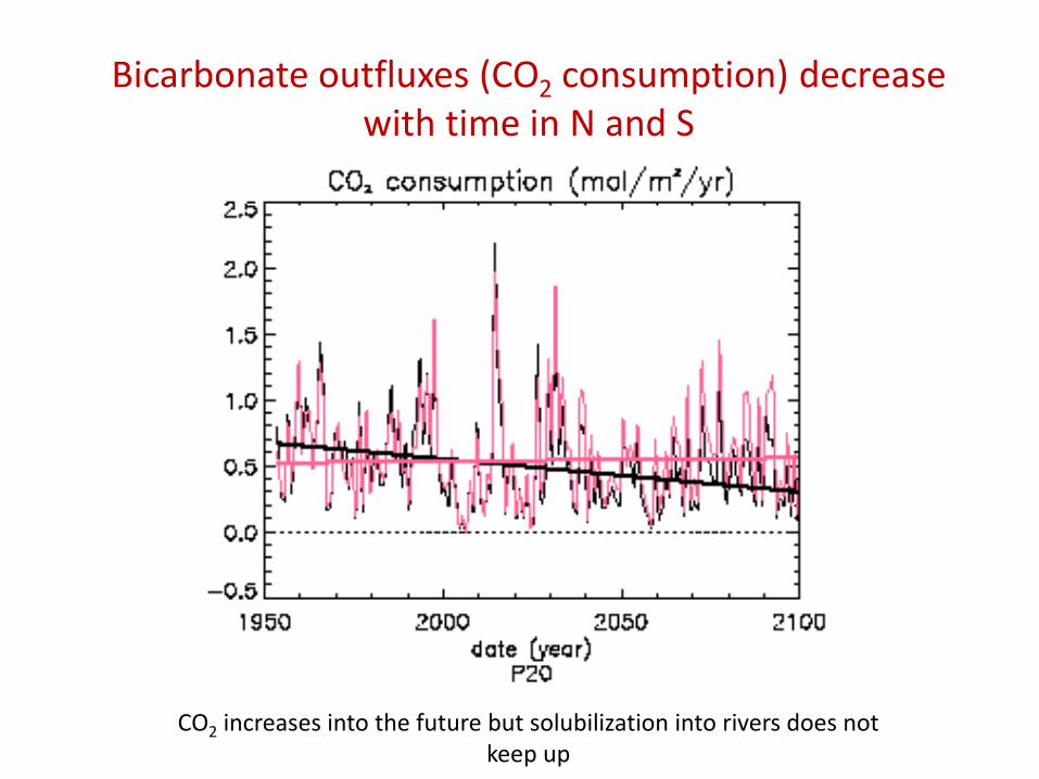
Bicarbonate outfluxes (CO2 consumption) decrease with time in N and S

CO2 increases into the future but solubilization into rivers does not keep up

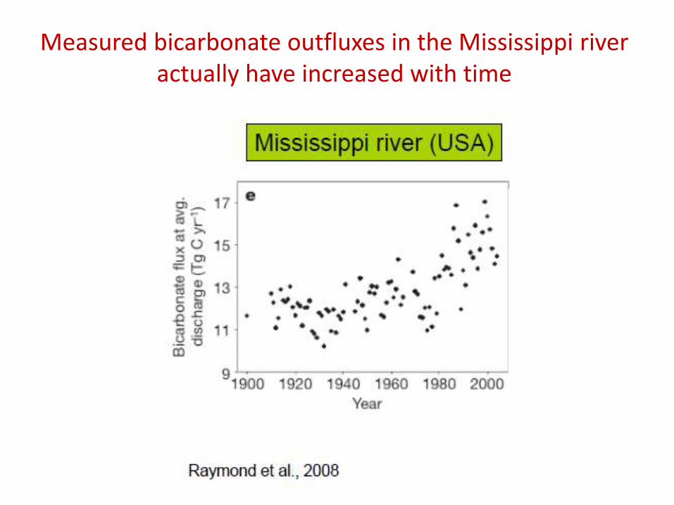
Measured bicarbonate outfluxes in the Mississippi river actually have increased with time

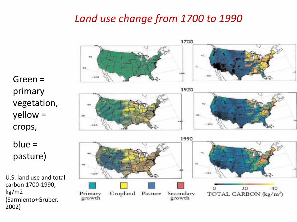
Land use change from 1700 to 1990

U.S. land use and total carbon 1700-1990, kg/m2 (Sarmiento+Gruber, 2002)

Green = primary vegetation, yellow = crops,

blue = pasture)

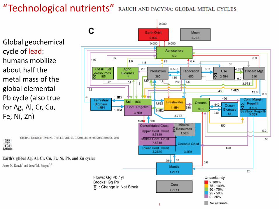
Global geochemical cycle of lead: humans mobilize about half the metal mass of the global elemental Pb cycle (also true for Ag, Al, Cr, Cu, Fe, Ni, Zn)

“Technological nutrients”

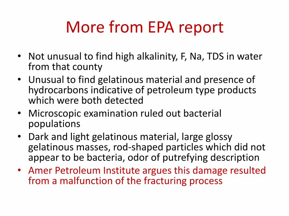
• Not unusual to find high alkalinity, F, Na, TDS in water from that county

• Unusual to find gelatinous material and presence of hydrocarbons indicative of petroleum type products which were both detected

• Microscopic examination ruled out bacterial populations

• Dark and light gelatinous material, large glossy gelatinous masses, rod-shaped particles which did not appear to be bacteria, odor of putrefying description

• Amer Petroleum Institute argues this damage resulted from a malfunction of the fracturing process

More from EPA report

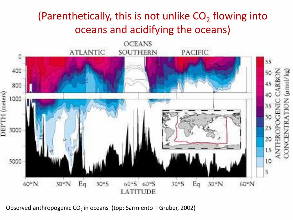
Observed anthropogenic CO2 in oceans (top: Sarmiento + Gruber, 2002)

(Parenthetically, this is not unlike CO2 flowing into oceans and acidifying the oceans)

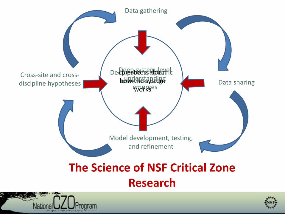
Data gathering

The Science of NSF Critical Zone Research

Data sharing

Model development, testing, and refinement

Cross-site and cross-discipline hypotheses

Deep process-specific understanding

Questions about how the system

works

Deep system-level understanding

emerges

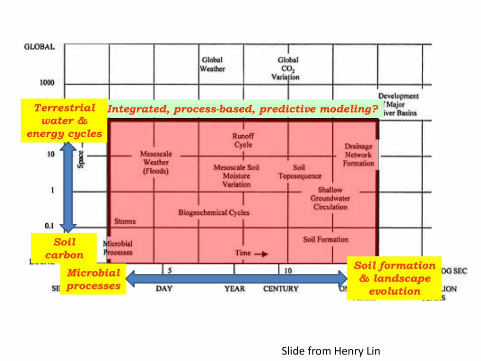
Integrated, process-based, predictive modeling?

Microbial

processes

Soil formation

& landscape

evolution

Soil

carbon

Terrestrial

water &

energy cycles

Slide from Henry Lin

Documents

Earthcasting the Future of the Critical Zonedels.nas.edu/resources/static-assets/besr/miscellaneous/Brantley.pdf · Earthcasting the Future of the ... Syncrude - a joint venture of