ECE 4680 DSP Laboratory 4: FIR Digital · PDF fileECE 4680 DSP Laboratory 4: FIR Digital Filters Problems 3 an analog filter. In particular, we can use this equipment to characterize

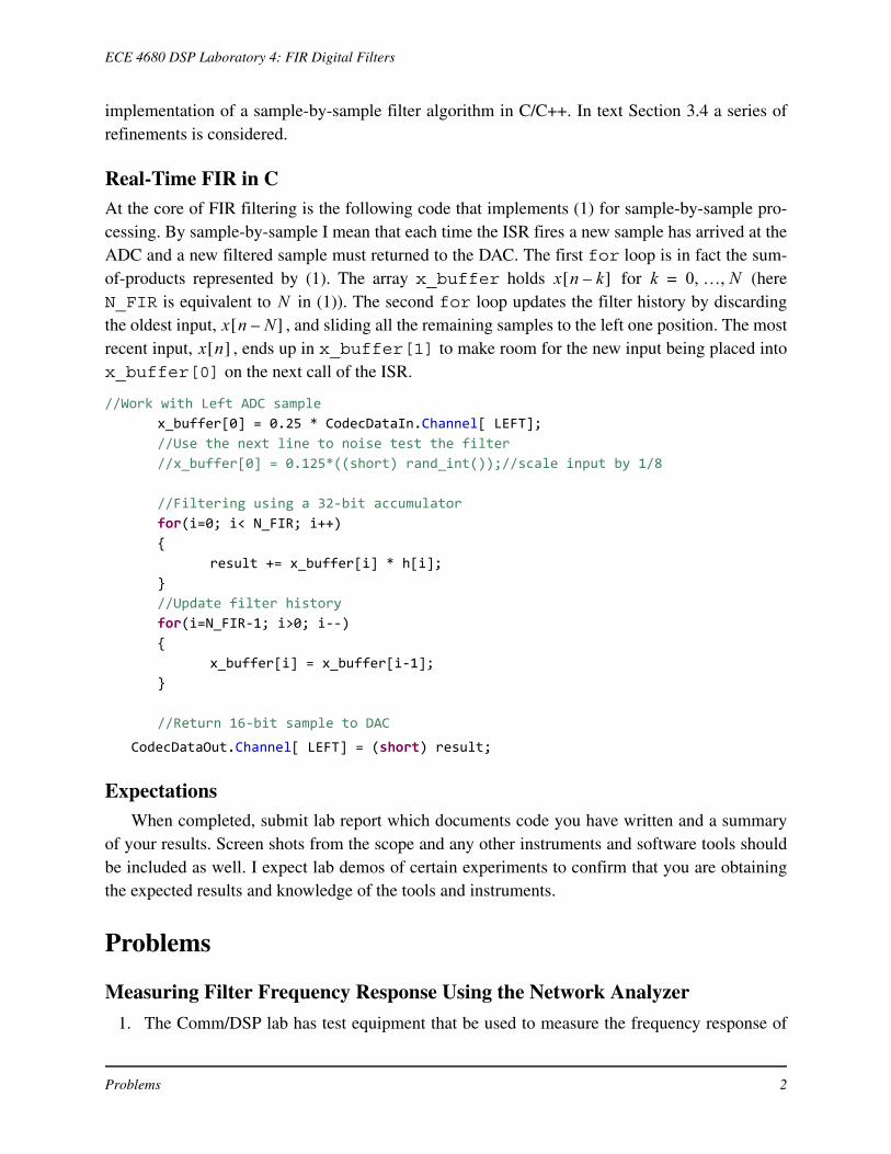
ECE 4680 DSP Laboratory 4: FIR Digital Filters

ECE 4680 DSP Laboratory 4:FIR Digital Filters

Due 12:15 PM Friday October 31, 2014

Introduction

Finite Impulse Response BasicsChapter 3 of the course text deals with FIR digital filters. In ECE 2610 considerable time wasspent with this class of filter. Recall that the difference equation for filtering input with filtercoefficient set , is

. (1)

The number of filter coefficients (taps) is and the filter order is . The coefficients are typ-ically obtained using MATLAB’s filter design function, fdatool(). The filter impulse responseis

(2)

the filter frequency response is

(3)

and the filter system function (z-domain representation) is

. (4)

From the system function it is clear why the filter order is N. The highest negative power of z is N.

Once a set of filter coefficients is available an FIR filter can make use of them. In MATLAB

code this is easy since we have the filter() function available. In MATLAB suppose x is a vec-tor input signal values that we want to filter and vector h contains the FIR coefficients. We canobtain the filtered output vector y via

>> y = filter(h,1,x);

In this lab we move beyond the use of MATLAB for filtering signals, and consider the real-time

x n[ ]b n[ ] n, 0 … N, ,=

y n[ ] h k[ ]x n k–[ ]k 0=

N

=

N 1+ N

h n[ ] h k[ ]δ n k–[ ]k 0=

N

=

H ejω( ) h k[ ]e jkω–

k 0=

N

=

H z( ) h k[ ]z 1–

k 0=

N

h 0[ ] h 1[ ]z 1– … h N[ ]z N–+ + += =

Introduction 1


implementation of a sample-by-sample filter algorithm in C/C++. In text Section 3.4 a series ofrefinements is considered.

Real-Time FIR in CAt the core of FIR filtering is the following code that implements (1) for sample-by-sample pro-cessing. By sample-by-sample I mean that each time the ISR fires a new sample has arrived at theADC and a new filtered sample must returned to the DAC. The first for loop is in fact the sum-of-products represented by (1). The array x_buffer holds for (hereN_FIR is equivalent to in (1)). The second for loop updates the filter history by discardingthe oldest input, , and sliding all the remaining samples to the left one position. The mostrecent input, , ends up in x_buffer[1] to make room for the new input being placed intox_buffer[0] on the next call of the ISR.

//Work with Left ADC samplex_buffer[0] = 0.25 * CodecDataIn.Channel[ LEFT];//Use the next line to noise test the filter//x_buffer[0] = 0.125*((short) rand_int());//scale input by 1/8

//Filtering using a 32-bit accumulatorfor(i=0; i< N_FIR; i++){

result += x_buffer[i] * h[i];}//Update filter historyfor(i=N_FIR-1; i>0; i--){

x_buffer[i] = x_buffer[i-1];}

//Return 16-bit sample to DAC

CodecDataOut.Channel[ LEFT] = (short) result;

ExpectationsWhen completed, submit lab report which documents code you have written and a summary

of your results. Screen shots from the scope and any other instruments and software tools shouldbe included as well. I expect lab demos of certain experiments to confirm that you are obtainingthe expected results and knowledge of the tools and instruments.

Problems

Measuring Filter Frequency Response Using the Network Analyzer

1. The Comm/DSP lab has test equipment that be used to measure the frequency response of

x n k–[ ] k 0 … N, ,=N

x n N–[ ]x n[ ]

Problems 2


an analog filter. In particular, we can use this equipment to characterize the end-to-endresponse of a digital filter that sits inside of an A/D- -D/A processor, such as theOMAP-L138. The instructor will demonstrate how to properly use the Agilent 4395A vec-tor/spectrum analyzer for taking frequency response measurements of the WinDSK8 equal-izer app.

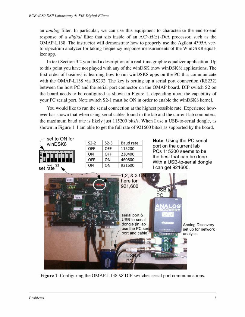
In text Section 3.2 you find a description of a real-time graphic equalizer application. Upto this point you have not played with any of the winDSK (now winDSK8) applications. Thefirst order of business is learning how to run winDSK8 apps on the PC that communicatewith the OMAP-L138 via RS232. The key is setting up a serial port connection (RS232)between the host PC and the serial port connector on the OMAP board. DIP switch S2 onthe board needs to be configured as shown in Figure 1, depending upon the capability ofyour PC serial port. Note switch S2-1 must be ON in order to enable the winDSK8 kernel.

You would like to run the serial connection at the highest possible rate. Experience how-ever has shown that when using serial cables found in the lab and the current lab computers,the maximum baud rate is likely just 115200 bits/s. When I use a USB-to-serial dongle, asshown in Figure 1, I am able to get the full rate of 921600 bits/s as supported by the board.

H z( )

{

S2-2 S2-3 Baud rate OFF OFF 115200 ON OFF 230400 OFF ON 460800 ON ON 921600

Note: Using the PC serialport on the current labPCs 115200 seems to bethe best that can be done.With a USB-to-serial dongleI can get 921600.

serial port &USB-to-serialdongle (in labuse the PC serialport and cable)

Analog Discoveryset up for networkanalysis

Figure 1: Configuring the OMAP-L138 s2 DIP switches serial port communications.

USB toPC

USB toPC

set to ON forwinDSK8

1,2, & 3 ONhere for921,600

set rate

Problems 3


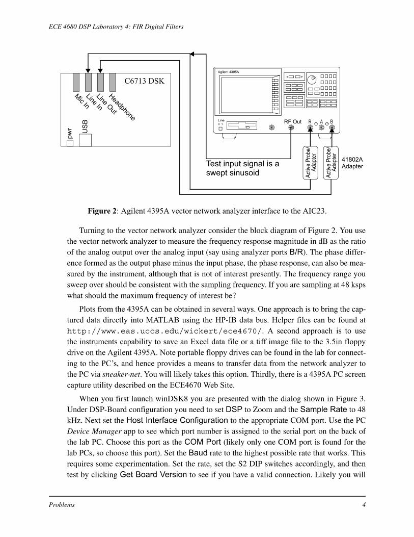
Turning to the vector network analyzer consider the block diagram of Figure 2. You usethe vector network analyzer to measure the frequency response magnitude in dB as the ratioof the analog output over the analog input (say using analyzer ports B/R). The phase differ-ence formed as the output phase minus the input phase, the phase response, can also be mea-sured by the instrument, although that is not of interest presently. The frequency range yousweep over should be consistent with the sampling frequency. If you are sampling at 48 kspswhat should the maximum frequency of interest be?

Plots from the 4395A can be obtained in several ways. One approach is to bring the cap-tured data directly into MATLAB using the HP-IB data bus. Helper files can be found athttp://www.eas.uccs.edu/wickert/ece4670/. A second approach is to usethe instruments capability to save an Excel data file or a tiff image file to the 3.5in floppydrive on the Agilent 4395A. Note portable floppy drives can be found in the lab for connect-ing to the PC’s, and hence provides a means to transfer data from the network analyzer tothe PC via sneaker-net. You will likely takes this option. Thirdly, there is a 4395A PC screencapture utility described on the ECE4670 Web Site.

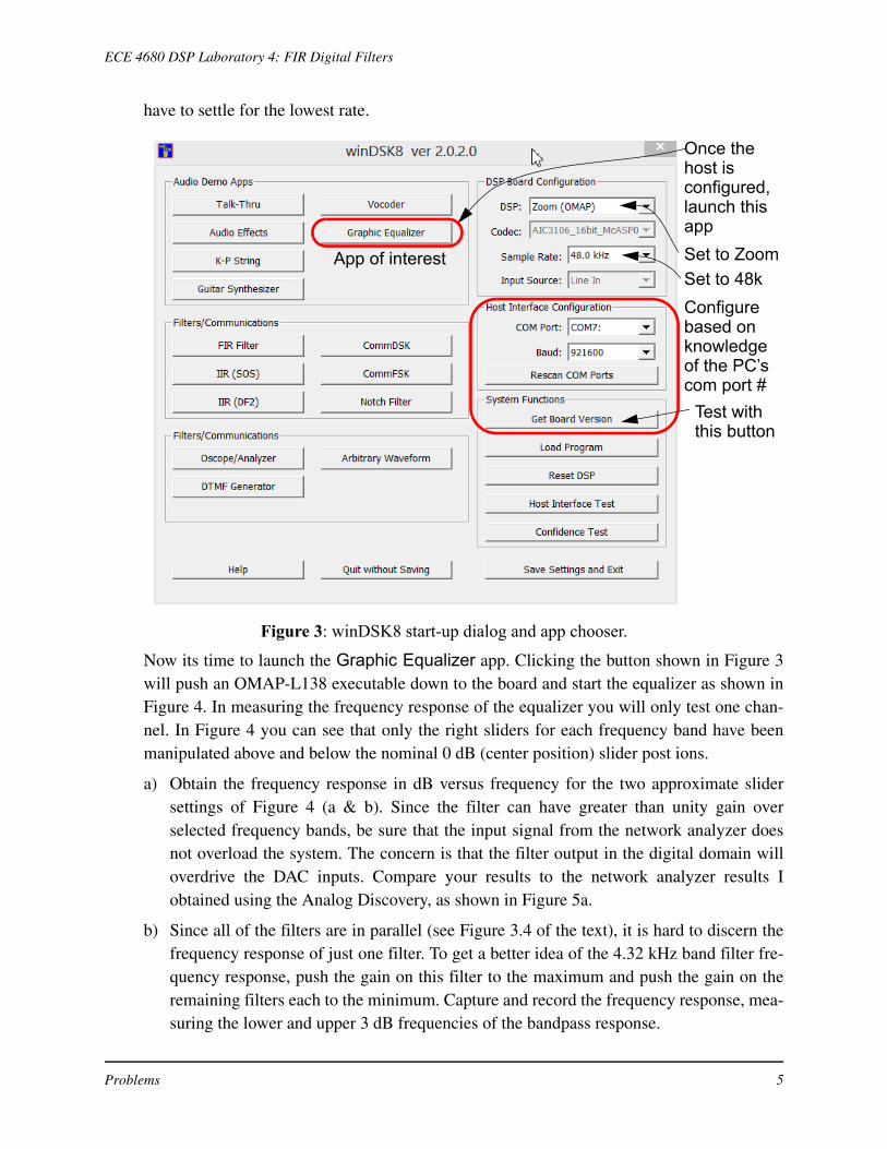
When you first launch winDSK8 you are presented with the dialog shown in Figure 3.Under DSP-Board configuration you need to set DSP to Zoom and the Sample Rate to 48kHz. Next set the Host Interface Configuration to the appropriate COM port. Use the PCDevice Manager app to see which port number is assigned to the serial port on the back ofthe lab PC. Choose this port as the COM Port (likely only one COM port is found for thelab PCs, so choose this port). Set the Baud rate to the highest possible rate that works. Thisrequires some experimentation. Set the rate, set the S2 DIP switches accordingly, and thentest by clicking Get Board Version to see if you have a valid connection. Likely you will

Figure 2: Agilent 4395A vector network analyzer interface to the AIC23.

Agilent 4395A

0 1 . . . .RF OutLine R BA

Activ

e Pr

obe/

Adap

ter

41802AAdapter

pwr USB

Mic InLine In

Line Out

Headphone

C6713 DSK

Activ

e Pr

obe/

Adap

ter

Test input signal is aswept sinusoid

Problems 4


have to settle for the lowest rate.

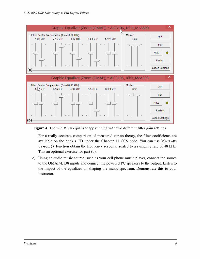
Now its time to launch the Graphic Equalizer app. Clicking the button shown in Figure 3will push an OMAP-L138 executable down to the board and start the equalizer as shown inFigure 4. In measuring the frequency response of the equalizer you will only test one chan-nel. In Figure 4 you can see that only the right sliders for each frequency band have beenmanipulated above and below the nominal 0 dB (center position) slider post ions.

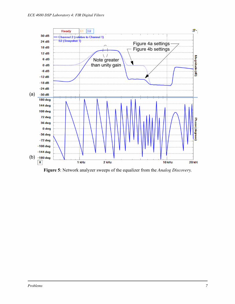
a) Obtain the frequency response in dB versus frequency for the two approximate slidersettings of Figure 4 (a & b). Since the filter can have greater than unity gain overselected frequency bands, be sure that the input signal from the network analyzer doesnot overload the system. The concern is that the filter output in the digital domain willoverdrive the DAC inputs. Compare your results to the network analyzer results Iobtained using the Analog Discovery, as shown in Figure 5a.

b) Since all of the filters are in parallel (see Figure 3.4 of the text), it is hard to discern thefrequency response of just one filter. To get a better idea of the 4.32 kHz band filter fre-quency response, push the gain on this filter to the maximum and push the gain on theremaining filters each to the minimum. Capture and record the frequency response, mea-suring the lower and upper 3 dB frequencies of the bandpass response.

App of interestSet to 48kConfigurebased onknowledgeof the PC’scom port #

Test withthis button

Once thehost isconfigured,launch thisapp

Figure 3: winDSK8 start-up dialog and app chooser.

Set to Zoom

Problems 5


For a really accurate comparison of measured versus theory, the filter coefficients areavailable on the book’s CD under the Chapter 11 CCS code. You can use MATLABsfreqz() function obtain the frequency response scaled to a sampling rate of 48 kHz.This an optional exercise for part (b).

c) Using an audio music source, such as your cell phone music player, connect the sourceto the OMAP-L138 inputs and connect the powered PC speakers to the output. Listen tothe impact of the equalizer on shaping the music spectrum. Demonstrate this to yourinstructor.

Figure 4: The winDSK8 equalizer app running with two different filter gain settings.

(a)

(b)

Problems 6


(a)

(b)

Figure 4a settingsFigure 4b settings

Figure 5: Network analyzer sweeps of the equalizer from the Analog Discovery.

Note greaterthan unity gain

Problems 7


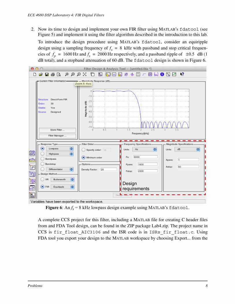
2. Now its time to design and implement your own FIR filter using MATLAB’s fdatool (seeFigure 5) and implement it using the filter algorithm described in the introduction to this lab.

To introduce the design procedure using MATLAB’s fdatool, consider an equirippledesign using a sampling frequency of kHz with passband and stop critical frequen-cies of Hz and Hz respectively, and a passband ripple of dB (1dB total), and a stopband attenuation of 60 dB. The fdatool design is shown in Figure 6.

A complete CCS project for this filter, including a MATLAB file for creating C header filesfrom and FDA Tool design, can be found in the ZIP package Lab4.zip. The project name inCCS is fir_float_AIC3106 and the ISR code is in ISRs_fir_float.c. UsingFDA tool you export your design to the MATLAB workspace by choosing Export... from the

fs 8=fp 1600= fs 2000= 0.5±

Figure 6: An fs = 8 kHz lowpass design example using MATLAB’s fdatool.

Designrequirements

Problems 8


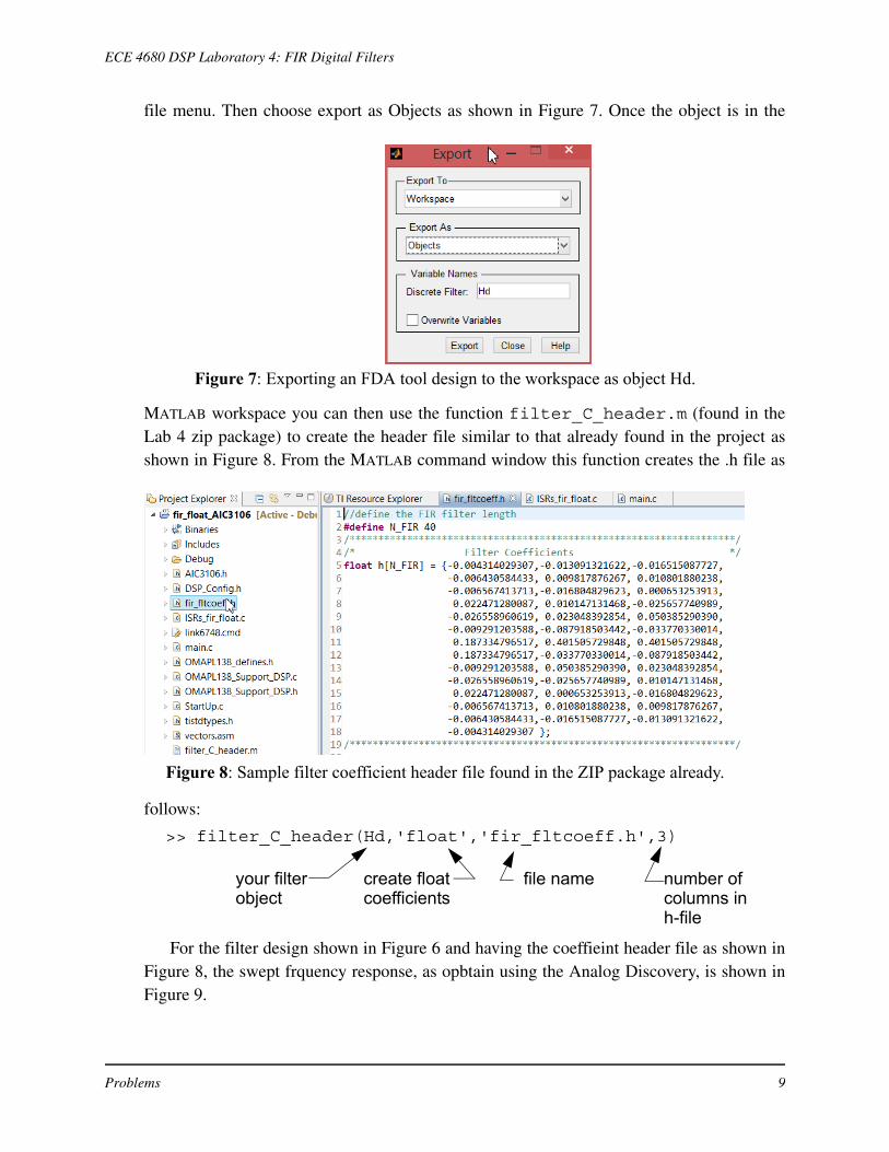
file menu. Then choose export as Objects as shown in Figure 7. Once the object is in the

MATLAB workspace you can then use the function filter_C_header.m (found in theLab 4 zip package) to create the header file similar to that already found in the project asshown in Figure 8. From the MATLAB command window this function creates the .h file as

follows:

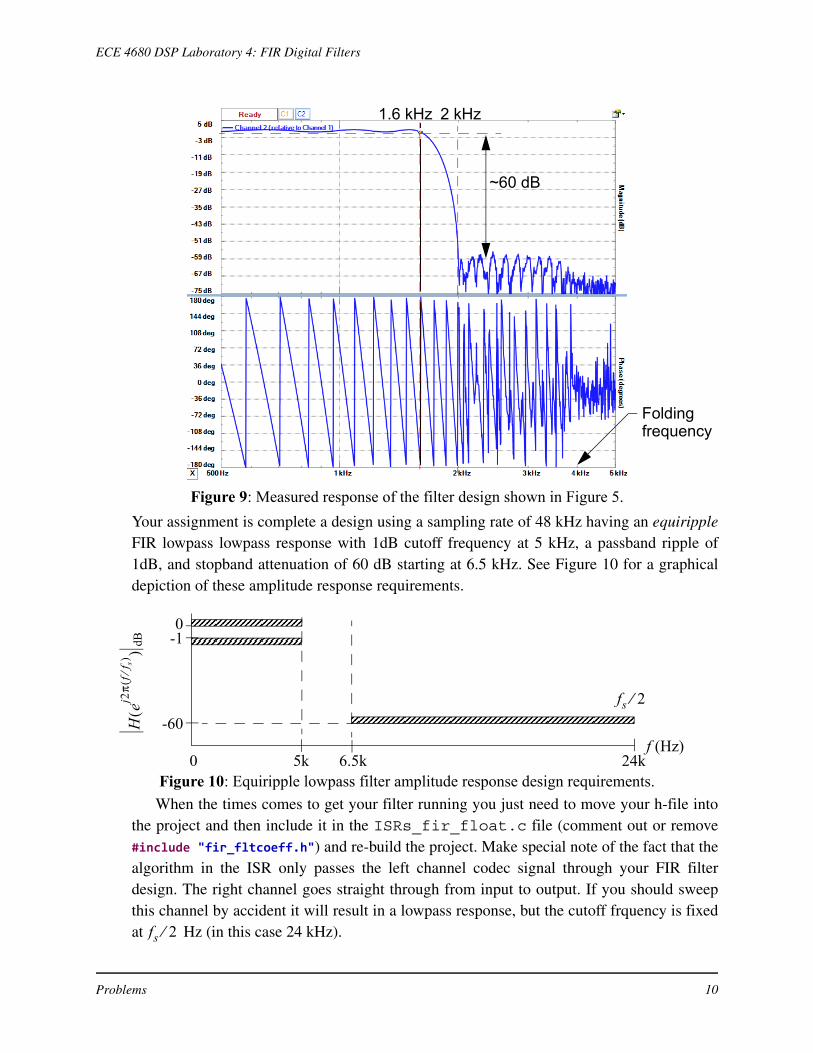
For the filter design shown in Figure 6 and having the coeffieint header file as shown inFigure 8, the swept frquency response, as opbtain using the Analog Discovery, is shown inFigure 9.

Figure 7: Exporting an FDA tool design to the workspace as object Hd.

Figure 8: Sample filter coefficient header file found in the ZIP package already.

>> filter_C_header(Hd,'float','fir_fltcoeff.h',3)

your filterobject

create floatcoefficients

file name number of columns inh-file

Problems 9


Your assignment is complete a design using a sampling rate of 48 kHz having an equirippleFIR lowpass lowpass response with 1dB cutoff frequency at 5 kHz, a passband ripple of1dB, and stopband attenuation of 60 dB starting at 6.5 kHz. See Figure 10 for a graphicaldepiction of these amplitude response requirements.

When the times comes to get your filter running you just need to move your h-file intothe project and then include it in the ISRs_fir_float.c file (comment out or remove#include "fir_fltcoeff.h") and re-build the project. Make special note of the fact that thealgorithm in the ISR only passes the left channel codec signal through your FIR filterdesign. The right channel goes straight through from input to output. If you should sweepthis channel by accident it will result in a lowpass response, but the cutoff frquency is fixedat Hz (in this case 24 kHz).

Figure 9: Measured response of the filter design shown in Figure 5.

Foldingfrequency

1.6 kHz 2 kHz

~60 dB

Figure 10: Equiripple lowpass filter amplitude response design requirements.

Hej2

πf

f s⁄(

)(

) dB

0-1

-60

0 5k 6.5k 24kf (Hz)

fs 2⁄

fs 2⁄

Problems 10


// A portion of ISRs_fir_float.cCodecDataIn.UINT = ReadCodecData();// get input data samples

//Work with Left ADC samplex_buffer[0] = 0.25 * CodecDataIn.Channel[ LEFT];//Use the next line to noise test the filter//x_buffer[0] = 0.125*((short) rand_int());//scale input by 1/8

//Filtering using a 32-bit accumulator ‘result’for(i=0; i< N_FIR; i++){

result += x_buffer[i] * h[i];}//Update filter historyfor(i=N_FIR-1; i>0; i--){

x_buffer[i] = x_buffer[i-1];}

//Return 16-bit sample to DACCodecDataOut.Channel[ LEFT] = (short) result;// Copy Right input directly to Right output with no filteringCodecDataOut.Channel[RIGHT] = CodecDataIn.Channel[ RIGHT];/* end your code here */WriteCodecData(CodecDataOut.UINT);// send output data to port

a) Using the network analyzer obtain the analog frequency response of your filter designand compare it with your theoretical expectations from FDA tool. Check the filter gain atthe passband and stopband critical frequencies to see how well hey match the theoreticaldesign results.

b) Measure the time spent in the ISR when running the FIR filter of part (a) when using -o3optimization. Recall your experiences with the digital output pin in Lab 3. Note that dig-ital I/O is enabled in this project. How much time do you have to spend in the ISR whensampling at 48 kHz? What is the maximum sampling rate you can operate your filter atand still meet real-time operation?

c) Suppose the total time spent in the ISR, call it , is composed of a fixed time compo-nent plus the time required to run the actual DSP algorithm, call it . Experi-mentally measure by bypassing the two for loops of the FIR filter routine. Theninfer from the two ISR time measurement you have made. Determine the maximumnumber of FIR coefficients the present algorithm can support with kHz and stillmeet real-time. Show your work. You can assume that grows linearly with the num-ber of coefficients, N_FIR.

TISRTfixed Talg

TfixedTalg

fs 48=Talg

Problems 11


Measuring Frequency Response Using White Noise Excitation

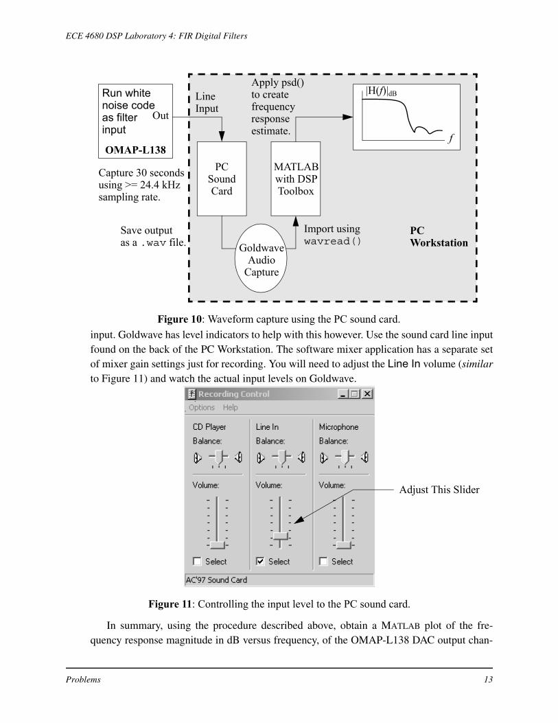
3. Rather than using the network analyzer as in Problems 1–2, this time you will use the PCdigital audio system to capture a finite record of DAC output as shown in Figure 10. Use thesame FIR filter as used in Problem 2. The software capture tool that is useful here is theshareware program GoldWave (goldwave.zip on Web site). A 30 second capture at 44.1kHz seems to work well. Since the sampling rate is only 32 ksps.

To get this setup you first need to add a function to your code so that you can digitallygenerate a noise source as the input to your filtering algorithm. Add the following uniformrandom number generator function to the ISR code module:

//White noise generator for filter noise testinglong int rand_int(void){

static long int a = 100001;

a = (a*125) % 2796203;return a;

}

Note the code is already in place in the project you extract from the Lab 4 zip file. Now youwill drive your filter algorithm with white noise generated via the function rand_int().In your filter code you will replace the read from the audio code with something like to fol-lowing:

//Work with Left ADC sample//x_buffer[0] = 0.25 * CodecDataIn.Channel[ LEFT];//Use the next line to noise test the filterx_buffer[0] = 0.125*((short) rand_int());//scale input by 1/8

Once a record is captured in GoldWave it can be saved as a .wav file. The .wav filecan then be loaded into MATLAB using the wavread() function. MATLAB has the abilityto import data files directly from the Import Data... option under the file menu. Note, Gold-Wave can directly display waveforms and their corresponding spectra, but higher qualityspectral analysis can be performed using the MATLAB signal processing toolbox. The spec-tral analysis function to be used in MATLAB is psd(), which implements Welch’s methodof averaged periodograms. Suppose that the .wav file is saved as test1.wav, then a plotof the frequency response would be created as follows:

>> [x,Fs] = wavread(‘test1.wav’); %Get x and sampling rate

>> % Use 2048 pt. FFT and plot with proper fs value

>> simpleSA(detrend(x),2048,48,-80,10); %detrend() removes DC offsets

>> % Rescale plot as needed and overlay other plots if desired.

Note the spectral estimation function simpleSA.m, which wraps psd(), can be found inthe zip package. One condition to watch out for is overloading of the PC sound card line

Problems 12


input. Goldwave has level indicators to help with this however. Use the sound card line inputfound on the back of the PC Workstation. The software mixer application has a separate setof mixer gain settings just for recording. You will need to adjust the Line In volume (similarto Figure 11) and watch the actual input levels on Goldwave.

In summary, using the procedure described above, obtain a MATLAB plot of the fre-quency response magnitude in dB versus frequency, of the OMAP-L138 DAC output chan-

OMAP-L138PC

SoundCard

Capture 30 secondsusing >= 24.4 kHzsampling rate.

Save outputas a .wav file.

MATLABwith DSPToolbox

Import usingwavread()

Apply psd()to createfrequencyresponseestimate. f

|H(f)|dB

PCWorkstation

LineInputOut

GoldwaveAudio

Capture

Figure 10: Waveform capture using the PC sound card.

Run whitenoise codeas filterinput

Adjust This Slider

Figure 11: Controlling the input level to the PC sound card.

Problems 13


nel. Normalize the filter gain so that it is unity at its peak frequency response magnitude.

Using a Circular Buffer

4. Implement the circular buffer as described in text Listing 3.6 into the filter design of Prob-lem 2. You will have to read through Section 3.4.3 of the text to get an understanding of thecircular buffer concept. The basic idea is trying to eliminate the update buffer history forloop. Using the real-time IRQ timing pulse see if you achieve any speed improvement under-o3 optimization. What is maximum number of filter coefficients you can handle at 48 kHz?

Problems 14


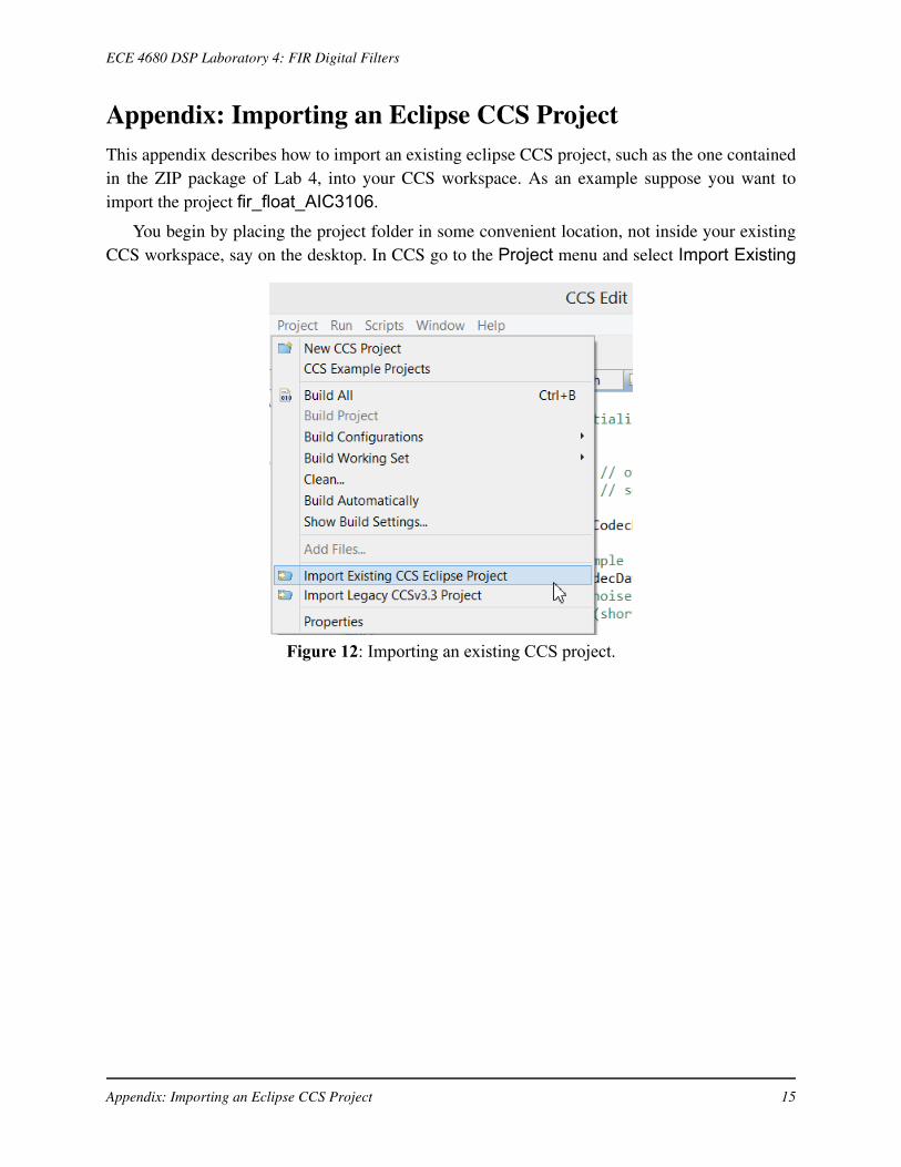
Appendix: Importing an Eclipse CCS ProjectThis appendix describes how to import an existing eclipse CCS project, such as the one containedin the ZIP package of Lab 4, into your CCS workspace. As an example suppose you want toimport the project fir_float_AIC3106.

You begin by placing the project folder in some convenient location, not inside your existingCCS workspace, say on the desktop. In CCS go to the Project menu and select Import Existing

Figure 12: Importing an existing CCS project.

Appendix: Importing an Eclipse CCS Project 15


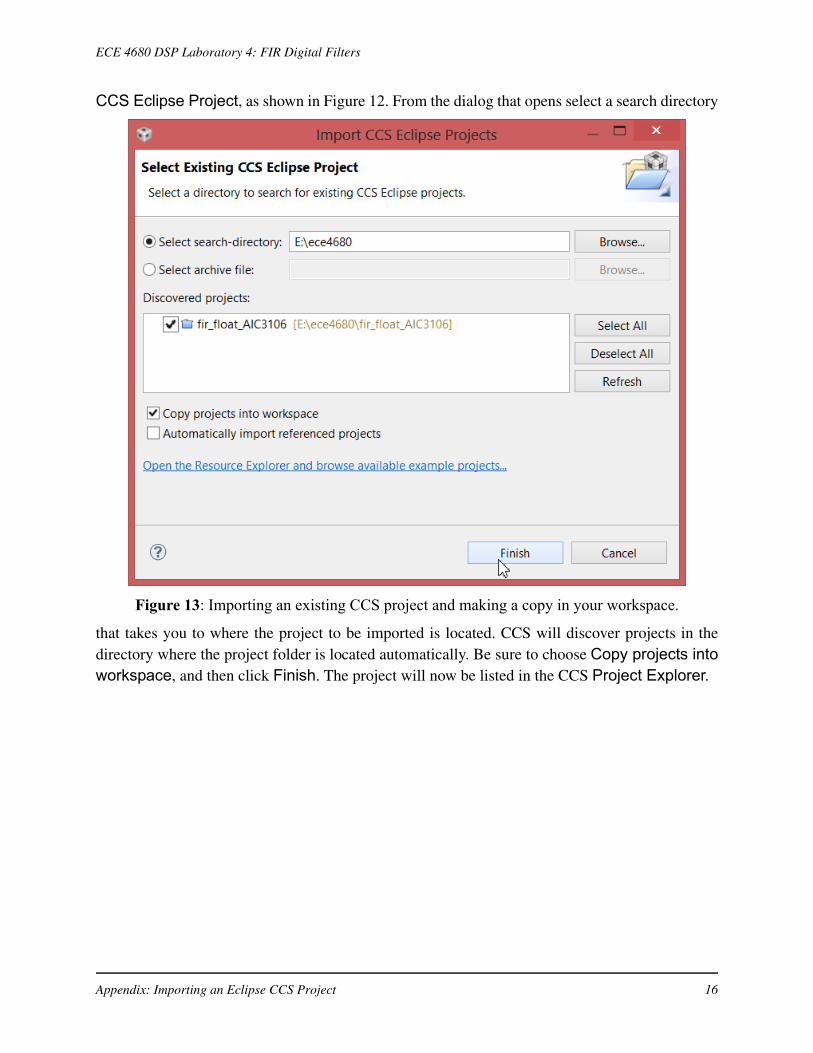
CCS Eclipse Project, as shown in Figure 12. From the dialog that opens select a search directory

that takes you to where the project to be imported is located. CCS will discover projects in thedirectory where the project folder is located automatically. Be sure to choose Copy projects intoworkspace, and then click Finish. The project will now be listed in the CCS Project Explorer.

Figure 13: Importing an existing CCS project and making a copy in your workspace.

Appendix: Importing an Eclipse CCS Project 16

Documents

ECE 4680 DSP Laboratory 4: FIR Digital · PDF fileECE 4680 DSP Laboratory 4: FIR Digital Filters Problems 3 an analog filter. In particular, we can use this equipment to characterize