Embed Size (px)
Citation preview

Efficient solution of a vibration equation involving
fractional derivativesAccepted Author’s Manuscript version of
International Journal of Non-Linear Mechanics 45:169–175, 2010
doi:10.1016/j.ijnonlinmec.2009.10.006
Attila Palfalvi
9 November 2009
Abstract
Fractional order (or, shortly, fractional) derivatives are used in viscoelasticity since thelate 1980s, and they grow more and more popular nowadays. However, their efficient numeri-cal calculation is nontrivial, because, unlike integer-order derivatives, they require evaluationof history integrals in every time step. Several authors tried to overcome this difficulty, eitherby simplifying these integrals or by avoiding them. In this paper, the Adomian decomposi-tion method is applied on a fractionally damped mechanical oscillator for a sine excitation,and the analytical solution of the problem is found. Also, a series expansion is derived whichproves very efficient for calculations of transients of fractional vibration systems. Numericalexamples are included.
Keywords: vibration , fractional derivative , fractional differential equation , Adomian de-composition
1 Introduction
It is common to date fractional calculus back to Leibniz, and several textbooks are available onthe subject (e.g. [26]). Several authors have been examining the possibility of using fractionalderivatives in material modelling in the last two-three decades [5; 6], and the field is of a grow-ing interest nowadays [1; 15–17; 27; 30]. Finite element formulations are also in development[8; 12; 30]. However, the wide spread of these models is obstructed among others by the diffi-culty concerning their efficient numerical calculation. This comes from the fact that they needthe evaluation of a time-history integral. There are several solution methods available in theliterature.
The analytical solution is theoretically known [26]. However, it requires the computationof a convolution of the two-parameter Mittag-Leffler function, which is numerically challenging.Therefore, other calculation methods are sought and used.
The most commonly used method is based on the well-known Grunwald–Letnikov definitionof fractional derivatives, used e.g. by Schmidt and Gaul [30]. These authors proceeded toreduce the volume of the time history integral [32], achieving an almost two-magnitude gain incalculation time on an example.
Suarez and Shokooh [35] solved a vibration equation with fractional damping of order 1/2analytically, taking advantage of the derivative order. Therefore, their solution is restricted tocases where the order of damping is one half. Still, the presented numerical results are widely
1

used as reference solutions. Moreover, Suarez and Shokooh presented a solution for the initialvalue problem of the vibration system, which is uncommon in the literature.
Yuan and Agrawal [38] have rewritten the definition of a fractional derivative, and turneda fractional differential equation to a system of linear differential equations. However, Schmidtand Gaul [31] have shown that in some cases, this method loses the advantages of fractionalcalculus over integer-order calculus. Later, this has also been checked by the present author [25]for the field of interest of this paper.
The Adomian decomposition method (ADM) has been introduced by George Adomian inthe late 1980s. Essentially, it approximates the solution of a non-linear differential equation witha series of functions. The method is getting into use for the solution of fractional differentialequations [9–11; 22; 29; 33; 36]. For a special case, Saha Ray, Poddar and Bera [29] have proventhat the Adomian solution converges to the analytical solution. Recently, Hu, Luo and Lu [19]have shown that this is true for any linear fractional differential equation. It will be shown inthe present paper that this series expansion is very efficient in many cases.
There are some further methods (e.g. the variational iteration method [23; 24], the methodof Atanackovic and Stankovic [2; 3] and the method of Singh and Chatterjee [34]) that will notbe treated in this paper. Also, the Adomian decomposition method has been improved by someauthors [20; 21; 28]. However, the convergence to the analytical solution has only been provenfor the original method.
The present paper aims to provide a computationally efficient solution method for the frac-tionally damped vibration equation using the Adomian decomposition method and Taylor series.The obtained solution will be compared to analytical solutions, either known previously or de-veloped here in a series form. To show the connection with classical methods, solutions usingthe Grunwald–Letnikov definition will also be calculated.
In this paper, Section 2 presents the fractionally damped vibration equation, also givinga brief introduction to fractional derivatives. It also describes the Adomian decompositionmethod which will be used afterwards. In Section 3, some solutions existing in the literature areshown. Next, in Section 4, new solutions are presented: in Section 4.1, the proposed methodis developed, while in Section 4.2, an analytical solution is calculated for reference. Finally,Section 5 shows the numerical examples, and Section 6 concludes the paper.
2 Preliminaries
This section gives the equation to be solved, including a basic introduction to fractional deriva-tives. The Adomian decomposition method, which is extensively used in this paper, is alsopresented.
2.1 The equation to be solved
The differential equation to be solved is the vibration equation with fractional damping, withone degree of freedom:
D2x(t) +c
mDαx(t) +
k
mx(t) = f(t) , (1)
where D =d
dtis the differential operator. Another common form of Equation (1) is
D2x(t) + 2ηω2−αn Dαx(t) + ω2
nx(t) = f(t) , (2)
with
2ηω2−αn =
c
mand ω2
n =k
m.
2

2.2 Fractional integrals
Fractional integrals and derivatives are deduced from the generalisation of the integer-orderoperations. It is usual to define the integral operator D−q as
aD−qt x(t) =
1
Γ(q)
∫ t
a(t− τ)q−1 x(τ) dτ , (3)
where q > 0 and Γ(x) is the Gamma function
Γ(x) =
∫
∞
0e−zzx−1 dz. (4)
For a continuous x(t),D−pD−qx(t) = D−(p+q)x(t) , (5)
as given in [26] (if both p and q are non-negative).The fractional integral of a polynomial will be needed later so it is given below:
D−qtν =Γ(ν + 1)
Γ(ν + 1 + q)tq+ν , (6)
With the fractional integral operator, fractional derivatives are easily introduced.
2.3 Fractional derivatives
For a real α > 0, Dα is defined by the Riemann–Liouville definition [26], using the abovefractional integral operator:
aDαt x(t) =
(
d
dt
)n
aD−(n−α)t x(t) =
1
Γ(n− α)
(
d
dt
)n ∫ t
a(t− τ)n−1−α x(τ) dτ . (7)
Another choice is the Caputo definition
CaD
αt x(t) =
1
Γ(n− α)
∫ t
a(t− τ)n−1−α
[(
d
dτ
)n
x(τ)
]
dτ . (8)
In both cases,(n− 1) < α < n.
Actually, the two definitions only differ in the consideration of conditions at the start of theinterval:
aDαt x(t) =
CaD
αt x(t) +
1
Γ (n− α)
n−1∑
k=0
Γ(n− α)
Γ(k − α+ 1)(t− a)k−α x(k)(a) . (9)
In the applications, D practically always means 0Dt, and most authors use the Riemann–Liouville, or the mathematically equivalent Grunwald–Letnikov definition (see [26] for preciseconditions of equivalence). Also, since the Riemann–Liouville definition has a singularity fornon-zero initial conditions, the initial conditions are often considered zero. For a physical inter-pretation of this singularity, see [18].
The composition (5) can be extended to an integral and a derivative:
D−pDqx(t) = DqD−px(t) = Dq−px(t) , (10)
with p, q ≥ 0 and a continuous x(t). (However, the composition of two fractional order deriva-tives is not straightforward.)
3

2.4 Adomian decomposition method
The decomposition method has been elaborated by George Adomian in the late 1980s, originallyfor non-linear differential equations. However, as mentioned in the introduction, it has also beenused by several authors for fractional differential equations [9–11; 22; 29; 33; 36]. As it will bealso used in this paper, it is presented in the followings.
The method has been described very clearly in [7]. The non-linear differential equation iswritten as:
Lx(t) + Rx(t) + Nx(t) = f(t) , (11)
where L is a linear operator which can be inverted easily, R is the remaining linear part and Nis a non-linear operator. The function x(t) is derived as a series expansion:
x(t) = x0(t) + x1(t) + x2(t) + . . . , (12)
usingx0(t) =
[
L−1Lx(t)− x(t)]
+ L−1f(t) (13)
andxn+1(t) = −L−1Rxn(t)− L−1An(t) (14)
with
An(t) =1
n!
[
dn
dλnN
(
∞∑
i=0
λixi(t)
)]
λ=0
. (15)
It has been proven recently by Hu, Luo and Lu [19] that for any linear fractional differentialequation, the solution given by the decomposition method converges to the analytical solution.Thus, Adomian decomposition is an adequate tool for solving such equations. In the followings,it will be shown that it can be very efficient, too.
3 Known solutions
This section presents solutions for the fractionally damped vibration equation (Section 2.1)which are well-established in the literature, and will be used here as reference solutions.
3.1 Analytical solution for α = 1/2
Suarez and Shokooh [35] calculate the analytical solution of Equation (2) for the special caseα = 1/2, both for a free vibration and a step function excitation. For the former, they obtain
xIC(t) =4∑
j=1
Ψ4jRj1√πt
+4∑
j=1
Ψ4jRjλjgj(t) , (16)
wheregj(t) = eλ
2
j t(
1 + erf(
λj
√t))
(17)
and λj and Ψj are the solution of the eigenproblem
AΨj = λjBΨj (18)
with
A =
0 0 1 00 1 0 01 0 0 00 0 0 −ω2
n
and B =
0 0 0 10 0 1 00 1 0 0
1 0 0 2ηω3/2n
,
4

and Ψ4j is the 4th coordinate of the jth eigenvector. In the above,
erf(x) =2√π
∫ x
0e−t2 dt
is the error function, and Rj comes from the initial conditions, by
R1
R2
R3
R4
=[
Ψ1 Ψ2 Ψ3 Ψ4
]
−1
v00x00
. (19)
The response to a step function force (using the Heaviside function H(t))
f(t) = f0H(t) ,
where X0 and V0 are considered zero, is
xH(t) = f0
4∑
j=1
Ψ24j
λj(gj(t)− 1) . (20)
For an arbitrary function f(t) and arbitrary initial conditions, the proposal of Suarez andShokooh is to consider the initial conditions according to the above. As for the force, theysuggest discretising the function and handling it as a series of step loads, one in each time step.However, with this method, the time history integral of the fractional derivative is replaced bya sum of displacement responses to step loads, which seems actually slower to calculate.
3.2 Grunwald–Letnikov formulation
It is common in the literature, especially in applications, to use the Grunwald–Letnikov definitionof a fractional derivative [26]:
Dαf(t) = limN→∞
(
t
N
)
−α N−1∑
j=0
Γ(j − α)
Γ(−α) Γ(j + 1)f
(
t− jt
N
)
. (21)
This, along with any time stepping scheme, allows to find a numerical solution for Equation (1).For simplicity, an explicit scheme has been used for time stepping in this paper:
vi+1 = vi + aih (22)
and
xi+1 = xi + vih+aih
2
2, (23)
where
ai = fi −k
mxi −
c
m
h−α
Γ(−α)
i−1∑
j=0
Γ(j − α)
Γ(j + 1)xi−j−1, (24)
h being the time step size and fi being the force per unit mass at t = ih.
4 New solutions
In this section, new solutions will be presented: first, an accurate and efficient series expansion,which is proposed for use; second, an analytical solution using the Adomian decompositionmethod as reference solution.
5

4.1 Proposed method: Taylor–Adomian series
The main goal of this paper is to propose a method for efficient calculation of the numericalsolution of Equation (1) with non-zero initial conditions. In the followings, this method will bepresented.
4.1.1 Description
In the proposed calculation method, Adomian decomposition is used, separately for initial con-ditions (starting displacement and velocity) and for the excitation. This can be done, as thedifferential operator defined in Section 2.3 is linear. The excitation is written in terms of Taylorseries, and the resulting method will be referred to as Taylor–Adomian series.
For our equation, a possible choice is
L = D2 , R =c
mDα +
k
mand N = 0.
In this case, conforming to Equations (13) and (14),
x0(t) =[
D−2D2x(t)− x(t)]
+D−2f(t) (25)
and
xn+1(t) = −k
mD−2xn(t)−
c
mDα−2xn(t) , (26)
the latter leading to
xn(t) =(−1)n
mn
n∑
j=0
(
n
j
)
cn−jkjD−((2−α)n+αj)x0(t) (27)
using the composition property (10) of an integral and a derivative operator.In Equation (25), the first term describes the contribution of initial conditions:
xIC0 (t) =[
D−2D2x(t)− x(t)]
= X0 + V0t, (28)
where X0 and V0 are the initial position and velocity, respectively. With Equations (27) and(6), one can write
xICn (t) =(−1)n
mnt(2−α)n
n∑
j=0
(
n
j
)
cn−jkjtjα(
X0
Γ(2n+ 1− (n− j)α)+
V0t
Γ(2n+ 2− (n− j)α)
)
. (29)
This result has also been obtained by Baclic and Atanackovic [4] using Laplace transformation.The second term of Equation (25) gives the response of the system to the excitation:
xf0(t) = D−2f(t) . (30)
Suppose an excitation of the form of the Taylor series
f(t) =∞∑
i=0
Titi, (31)
Tis being the coefficients of the polynomial. This, together with Equations (30) and (6), leadsto
xf0,i(t) = TiΓ(i+ 1)
Γ(i+ 3)ti+2 (32)
6

and
xfn,i(t) = Ti(−1)n
mnΓ(i+ 1) ti+(2−α)n+2
n∑
j=0
(
n
j
)
cn−jkj
Γ(i+ 3 + 2n− (n− j)α)tjα, (33)
xfn,i(t) being the nth term of the Adomian series of the response to the ith term of the Taylorseries of the excitation. The total response is
xf (t) =∞∑
n=0
∞∑
i=0
xfn,i(t) . (34)
Thus, the solution of Equation (1) has been given.
4.1.2 Technical considerations
The implementation of the method raises several questions. First, this is a double series ex-pansion, which means that both the number of terms in the Taylor series and the number ofterms in the Adomian series have to be defined. Moreover, Equations (29) and (33) show thatterms tjα become large for a relatively small t, which means a need for computing the differenceof large numbers. Thus, the evaluation of x(t) requires a computational precision better thanusual.
In the calculation code prepared for this paper, the number of terms is increased dynamicallythroughout the calculation, based on error estimations from the next ninc terms of the series:if the sum of the next ninc terms is larger than a small limit (‘error goal’), then the number ofterms is increased by ninc, and the error estimation will be based on the following ninc terms.This is applied separately for both series.
Another point is the required computational effort. The first two terms of the sum inEquation (29) give
xIC(t) = X0 + V0t−c
m
X0
Γ(3− α)t2−α −
k
m
X0
Γ(3)t2 −
c
m
V0
Γ(4− α)t3−α −
k
m
V0
Γ(4)t3 ± . . . (35)
This shows that the exponent of t in the series expansion is either an integer or a real number,the latter being computationally expensive. However, if α is restricted to be rational, as
α =p
q
with p and q both integers, the right-hand side of Equation (35) becomes a polynomial for(
t1/q)
:
xIC(t) = X0 + V0
(
t1/q)q
−c
m
X0
Γ(3− α)
(
t1/q)2q−p
−k
m
X0
Γ(3)
(
t1/q)2q
−c
m
V0
Γ(4− α)
(
t1/q)3q−p
−k
m
V0
Γ(4)
(
t1/q)3q
± . . . (36)
This can be computed efficiently.
4.1.3 Examples
Step function excitation For an excitation with the Heaviside function H(t) of the form
f(t) = f0H(t) ,
solved by Suarez and Shokooh [35] for α = 1/2, only T0 is non-zero of the Tis, resulting in
xfn(t) = f0(−1)n
mnt(2−α)n+2
n∑
j=0
(
n
j
)
cn−jkj
Γ(3 + 2n− (n− j)α)tjα. (37)
This has also been obtained by Saha Ray, Poddar and Bera [29] for α = 1/2 using Adomiandecomposition (with a slightly different selection for L, R, and N).
7
Sine excitation For a sine excitation of the form
f(t) = f0 sin(ωet) ,
the Taylor coefficients are
Ti =
0 if i is even
(−1)(i−1)/2 f0ωie
i!if i is odd
.
Using i = 2h+ 1 gives
Th = (−1)hω2h+1e
(2h+ 1)!,
which, inserted into Equation (33), leads to
xfn,h(t) = f0(−1)n+h
mnω2h+1e t(2−α)n+3+2h
n∑
j=0
(
n
j
)
cn−jkj
Γ(4 + 2 (n+ h)− (n− j)α)tjα, (38)
also using the propertyΓ(n+ 1) = n!
of the Gamma function.
4.2 Analytical solution by Adomian decomposition
Equation (27) gives the nth term of the Adomian series of x(t) if the original differential equationis Equation (1). For a sine excitation
f(t) = f0 sin(ωet) ,
this yields to
xn(t) =(−1)n
mn
n∑
j=0
(
n
j
)
cn−jkjD−((2−α)n+αj)(
D−2f0 sin(ωet))
.
Using the definition (3) of the integral operator, one obtains
x0(t) =
∫ t
0(t− τ) sin(ωeτ) dτ =
1
ω2e
(ωet− sin(ωet)) . (39)
This leads to
xn(t) =(−1)n
mn
f0ω2e
n∑
j=0
(
n
j
)
cn−jkj1
Γ(q)
∫ t
0(t− τ)q−1 (ωeτ − sin(ωeτ)) dτ , (40)
whereq = (2− α)n+ αj.
This results in
xn(t) =(−1)n
mn
f0ω2e
n∑
j=0
(
n
j
)
cn−jkj1
Γ(q + 2)
√t ω1/2−q
e s3/2+q,1/2(ωet) , (41)
for n > 0, where sµ,ν(t) is the Lommel-function [37]
sµ,ν(t) = 1F2
(
1;1
2(µ− ν + 3) ,
1
2(µ+ ν + 3) ;−
1
4t2)
tµ+1
(µ+ 1)2 − ν2
8
with 1F2(a1; b1, b2; t) being the hypergeometric function
1F2(a1; b1, b2; t) =∞∑
k=0
(a1)k(b1)k (b2)k
tk
k!,
where (a)k is the Pochhammer symbol
(a)k =Γ(a+ k)
Γ(a).
This can be calculated numerically by any computer algebra system.To the author’s knowledge, this solution has not been calculated in the literature before.
5 Numerical examples
So far, existing (Section 3) and new (Section 4) methods for the solution of the fractionallydamped vibration equation have been presented. In this section, they will be tested and com-pared for some parameter sets.
5.1 Software
First, some details are given on software used for the calculations.The code for the Taylor–Adomian series is written in C. The computational precision is
assured by the GNU Multiple precision library [14] and one of its derivatives, MPFR [13].The Grunwald–Letnikov formulation is also implemented in C, but it uses the conventional
double-precision arithmetics.The analytical solution of Suarez and Shokooh (described in Section 3.1) has been calculated
using the Maple computer algebra system.Also, for the analytical solution described in Section 4.2, the Maple computer algebra system
has been used with Equations (12), (29) and (41). Precision was higher than double precision,usually 50 or 75 decimal digits have been set. The run-time increase of the number of Adomianterms, described for the Taylor–Adomian method, has also been used here, with an error goalof 10−25 for ten terms.
5.2 Problems and results
In the followings, numerical examples and their results will be presented and compared. For thelatter purpose, let us introduce an absolute error indicator ε as
ε =1
N
N∑
i=1
∣
∣
∣xnumi − xrefi
∣
∣
∣.
Six problems have been analysed, two using a unit step force and four with a harmonicexcitation. Table 1 resumes the parameters of the different examples. They lead to steady-stateamplitudes between 0.012 and 0.021. The treated time interval is from 0 to 5 seconds. Withthe Taylor–Adomian method, 10 000 values of x(t) have been calculated for each problem. Thefloating-point precision was adjusted by hand as the required error level needed it; it was either128 or 192 bits for all calculations on this time interval.
9

Parameters 1 1u 2 2u 3 4
m 1 1 1 1 1 1α 1/2 1/2 1/2 1/2 1/5 1/5ωn 10 10 10 10 10 10η 0.5 0.5 0.05 0.05 0.5 0.05f0 1 1 1 1 1 1ωe 4π — 4π — 4π 4πX0 0.25 0.25 0.25 0.25 0.25 0.25V0 0 0 0 0 0 0
Table 1: Numerical parameters of the examples. Problems 1u and 2u use a step functionexcitation.
5.2.1 Derivative of order 1/2, step function excitation (problems 1u and 2u)
Here, the reference solution is from Suarez and Shokooh (Section 3.1), and the same numericalparameters have been used as in [35] to reproduce the same results (Figure 1). Here, and inthe followings, only the reference solutions are plotted; other solutions are very near when notpractically identical to them.
−0.25
−0.2
−0.15
−0.1
−0.05
0
0.05
0.1
0.15
0.2
0.25
0 1 2 3 4 5
Dis
plac
emen
t
Time
Problem 1uProblem 2u
Figure 1: Solution curves for problems 1u and 2u.
Figure 2 shows the error indicator ε and the elapsed CPU time for the two problems. It isimmediate to see that, for the same computational effort, the Taylor–Adomian method offers amuch greater precision. (However, an engineering precision is assured by any of the methods.)
The difference of the calculation times for the Taylor–Adomian method comes from the differ-ence of numerical conditions (mostly, the dissipation factor η), which require different numbersof terms in the Adomian series. As one would expect, the calculation times of the method basedon the Grunwald–Letnikov formulation were not affected by the numerical parameters.
10

1e−22
1e−20
1e−18
1e−16
1e−14
1e−12
1e−10
1e−08
1e−06
0.0001
0.01
0.01 0.1 1 10 100 1000 10000
Err
or (ε
)
CPU time [s]
Grünwald−Letnikov (1u)Taylor−Adomian (1u)
Grünwald−Letnikov (2u)Taylor−Adomian (2u)
Figure 2: Comparison of methods for problems 1u and 2u (α = 1/2, step function excitation).
5.2.2 Derivative of order 1/2, harmonic excitation (problems 1 and 2)
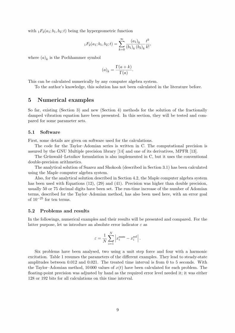
Here, the reference solution is the solution by Adomian decomposition (Section 4.2). Resultsare shown in Figure 3.
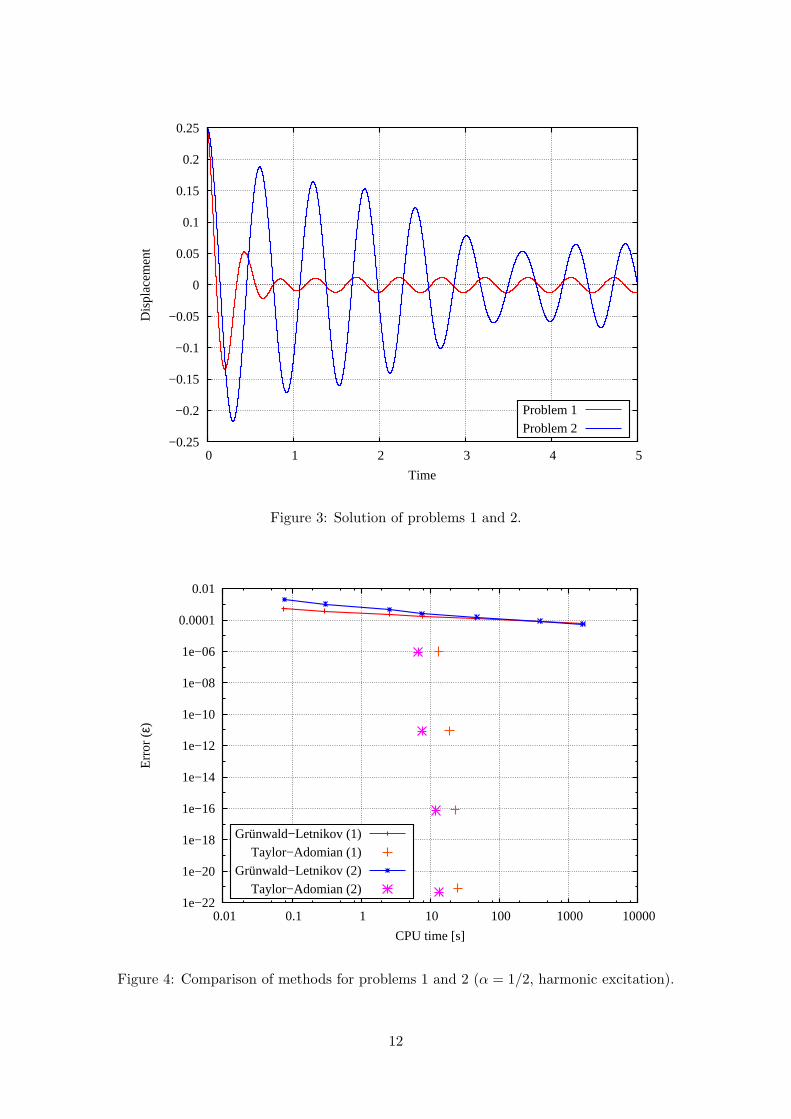
Error indicators and CPU times are shown in Figure 4. Observations are the same as above:for a calculation time of the 10-second order, the Taylor–Adomian method is much more precisethan the scheme with the Grunwald–Letnikov derivative.
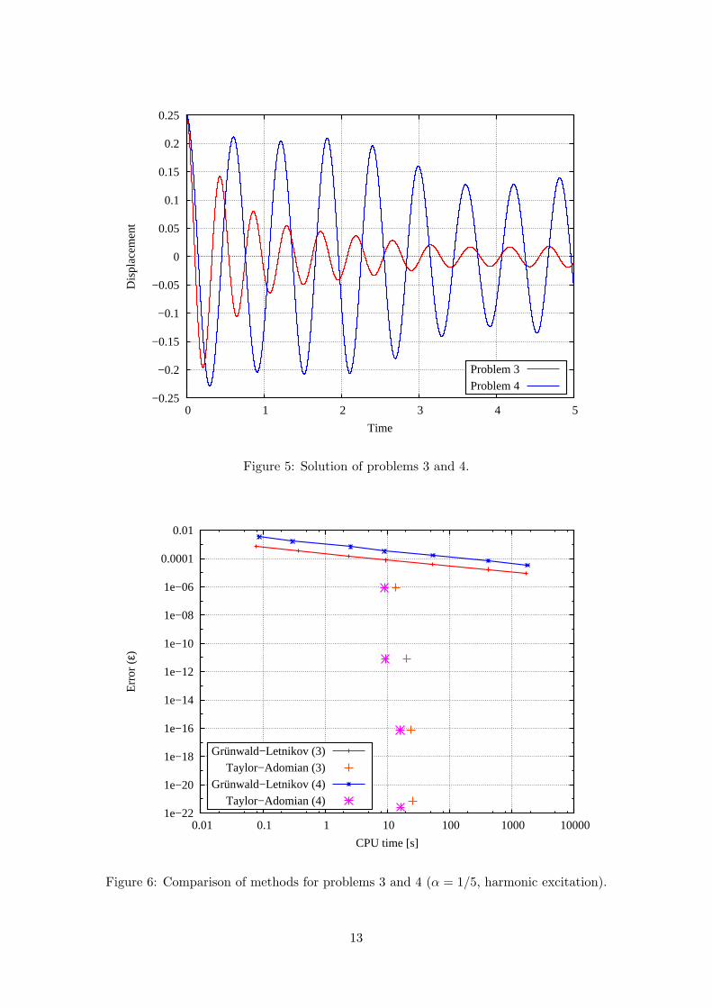
5.2.3 Derivative of order 1/5, harmonic excitation (problems 3 and 4)
To leave derivatives of order 1/2, another value has been chosen for α. The reference solutionfor these problems is the solution by Adomian decomposition (Section 4.2).
Results are shown in Figure 5, while Figure 6 shows the values of the error indicator andCPU times. It is immediate to see the same as before: the Taylor–Adomian method is clearlymuch more precise while keeping the calculation time low.
5.3 Simulating a longer time interval
As seen above, the terms of Equations (29) and (33) become very large as t increases. It is easyto see that a major limitation of the Taylor–Adomian method will be this property: beyonda certain interval length, a huge number of terms are required, which increases the calculationtime horrendously.
To check the extents of this phenomenon, calculations have been run with the Taylor–Adomian method up to the end of the transient, but at least to t = 25, with 200 calculatedpoints per time unit. The error goal was 10−10. Figure 7 shows elapsed CPU time versus simu-lated time. The points are at the end of the transient period, which is considered to be the end
11
−0.25
−0.2
−0.15
−0.1
−0.05
0
0.05
0.1
0.15
0.2
0.25
0 1 2 3 4 5
Dis
plac
emen
t
Time
Problem 1Problem 2
Figure 3: Solution of problems 1 and 2.
1e−22
1e−20
1e−18
1e−16
1e−14
1e−12
1e−10
1e−08
1e−06
0.0001
0.01
0.01 0.1 1 10 100 1000 10000
Err
or (ε
)
CPU time [s]
Grünwald−Letnikov (1)Taylor−Adomian (1)
Grünwald−Letnikov (2)Taylor−Adomian (2)
Figure 4: Comparison of methods for problems 1 and 2 (α = 1/2, harmonic excitation).
12
−0.25
−0.2
−0.15
−0.1
−0.05
0
0.05
0.1
0.15
0.2
0.25
0 1 2 3 4 5
Dis
plac
emen
t
Time
Problem 3Problem 4
Figure 5: Solution of problems 3 and 4.
1e−22
1e−20
1e−18
1e−16
1e−14
1e−12
1e−10
1e−08
1e−06
0.0001
0.01
0.01 0.1 1 10 100 1000 10000
Err
or (ε
)
CPU time [s]
Grünwald−Letnikov (3)Taylor−Adomian (3)
Grünwald−Letnikov (4)Taylor−Adomian (4)
Figure 6: Comparison of methods for problems 3 and 4 (α = 1/5, harmonic excitation).
13

of the last period of excitation for which the error indicator
1
N
N∑
i=1
∣
∣
∣xi − xsteadyi
∣
∣
∣
is above 1% of the steady-state amplitude.It is immediate to see that problems 1 and 3, i.e. the highly damped equations settle very
fast, and their CPU time for a very high precision is in the order of some or some 10 seconds.Even problem 2 settles within a CPU time of less than 10 minutes on an average 64-bit system.Contrarily, the transient of problem 4 required somewhat more than 6 hours to calculate on thesame computer. This shows that the presented Taylor–Adomian method may be very efficientfor the accurate solution of the fractionally damped vibration equation, especially when dampingis not very weak.
1
10
100
1000
10000
100000
5 10 20 30 40 50
CP
U ti
me
[s]
Simulated time
Problem 1Problem 2Problem 3Problem 4
Figure 7: Calculation times for longer time intervals.
6 Conclusion
In this paper, the main goal was to present a method to solve the fractionally damped, inho-mogeneous 1-DOF vibration equation with initial conditions. The Taylor–Adomian method hasbeen proposed and tested on step-function excited and harmonically excited cases. It has provenvery efficient in calculating the solution for a reasonably long time interval, practically with anarbitrarily low error. This makes the method immediately usable in providing quick referenceresults for other methods. The engineering application may be limited, however, due to thenecessity of high-precision arithmetics and the fast increase of calculation time as the simulatedtime interval gets longer.
Moreover, the analytical solution of the same equation (with a harmonic excitation) has beencalculated by the Adomian decomposition method. This solution served as a reference for the
14
Taylor–Adomian method.
Acknowledgement
The author would like to thank Prof. Laszlo Szabo for his encouragement and most helpfulcomments.
References
[1] Magnus Alvelid and Mikael Enelund. Modelling of constrained thin rubber layer withemphasis on damping. J. Sound Vibr., 300:662–675, 2007.
[2] T. M. Atanackovic and B. Stankovic. An expansion formula for fractional derivatives andits application. Fractional Calc. Appl. Anal., 7:365–378, 2004.
[3] T. M. Atanackovic and B. Stankovic. On a numerical scheme for solving differential equa-tions of fractional order. Mech. Res. Commun., 35:429–438, 2008.
[4] B. S. Baclic and T. M. Atanackovic. Stability and creep of a fractional derivative orderviscoelastic rod. Bull. Acad. Serb. Sci. Arts, CXXI:115–131, 2000.
[5] R. L. Bagley and P. J. Torvik. A theoretical basis for the application of fractional calculusto viscoelasticity. J. Rheol., 27:201–210, 1983.
[6] R. L. Bagley and P. J. Torvik. On the fractional calculus model of viscoelastic behavior. J.Rheol., 30:133–155, 1986.
[7] Wenhai Chen and Zhengyi Lu. An algorithm for Adomian decomposition method. Appl.
Math. Comput., 159:221–235, 2004.
[8] Fernando Cortes and Marıa Jesus Elejabarrieta. Homogenised finite element for transientdynamic analysis of unconstrained layer damping beams involving fractional derivative mod-els. Comput. Mech., 40:313–324, 2007.
[9] Varsha Daftardar-Gejji and Sachin Bhalekar. Solving multi-term linear and non-lineardiffusion–wave equations of fractional order by Adomian decomposition method. Appl.
Math. Comput., 202:113–120, 2008.
[10] Varsha Daftardar-Gejji and Hossein Jafari. Adomian decomposition: a tool for solving asystem of fractional differential equations. J. Math. Anal. Appl., 301:508–518, 2005.
[11] Varsha Daftardar-Gejji and Hossein Jafari. Solving a multi-order fractional differentialequation using Adomian decomposition. Appl. Math. Comput., 189:541–548, 2007.
[12] M. Enelund and G. A. Lesieutre. Time domain modeling of damping using anelastic dis-placement fields and fractional calculus. Int. J. Solids Struct., 36:4447–4472, 1999.
[13] Laurent Fousse, Guillaume Hanrot, Vincent Lefevre, Patrick Pelissier, and Paul Zimmer-mann. MPFR: A multiple-precision binary floating-point library with correct rounding.ACM Trans. Math. Softw., 33(2):13:1–13:15, 2007.
[14] Free Software Foundation, Inc. GNU multiple precision arithmetic library, version 4.2.4,2008.
15

[15] A. D. Freed and K. Diethelm. Fractional calculus in biomechanics: A 3D viscoelastic modelusing regularized fractional derivative kernels with application to the human calcaneal fatpad. Biomech. Model. Mechanobiol., 5:203–215, 2006.
[16] J. Hernandez-Santiago, A. Macias-Garcia, A. Hernandez-Jimenez, and J. Sanchez-Gonzalez.Relaxation modulus in PMMA and PTFE fitting by fractional Maxwell model. Polym. Test.,21:325–331, 2002.
[17] Nicole Heymans. Fractional calculus description of non-linear viscoelastic behaviour ofpolymers. Nonlinear Dyn., 38:221–231, 2004.
[18] Nicole Heymans and Igor Podlubny. Physical interpretation of initial conditions for frac-tional differential equations with Riemann–Liouville fractional derivatives. Rheologica Acta,45:765–771, 2006.
[19] Yizheng Hu, Yong Luo, and Zhengyi Lu. Analytical solution of the linear fractional differ-ential equation by Adomian decomposition method. J. Comput. Appl. Math., 215:220–229,2008.
[20] Hossein Jafari and Varsha Daftardar-Gejji. Revised Adomian decomposition method forsolving a system of nonlinear equations. Appl. Math. Comput., 175:1–7, 2006.
[21] Hossein Jafari and Varsha Daftardar-Gejji. Revised Adomian decomposition method forsolving systems of ordinary and fractional differential equations. Appl. Math. Comput.,181:598–608, 2006.
[22] Shaher Momani. A numerical scheme for the solution of multi-order fractional differentialequations. Appl. Math. Comput., 182:761–770, 2006.
[23] Shaher Momani and Zaid Odibat. Numerical approach to differential equations of fractionalorder. J. Comput. Appl. Math., 207:96–110, 2007.
[24] Shaher Momani and Zaid Odibat. Numerical comparison of methods for solving lineardifferential equations of fractional order. Chaos, Solitons & Fractals, 31:1248–1255, 2007.
[25] Attila Palfalvi. Methods for solving a semi-differential vibration equation. Period. Polytech.Ser. Mech. Eng., 51:1–5, 2007.
[26] Igor Podlubny. Fractional differential equations. Mathematics in Science and Engineering.Academic Press, 1999.
[27] Deepak S. Ramrakhyani, George A. Lesieutre, and Edward C. Smith. Modeling of elas-tomeric materials using nonlinear fractional derivative and continuously yielding frictionelements. Int. J. Solids Struct., 41:3929–3948, 2004.
[28] S. Saha Ray, K. S. Chaudhuri, and R. K. Bera. Application of modified decompositionmethod for the analytical solution of space fractional diffusion equation. Appl. Math. Com-
put., 196:294–302, 2008.
[29] S. Saha Ray, B. P. Poddar, and R. K. Bera. Analytical solution of a dynamic systemcontaining fractional derivative of order one-half by Adomian decomposition method. J.
Appl. Mech., 72:290–295, 2005.
[30] Andre Schmidt and Lothar Gaul. Finite element formulation of viscoelastic constitutiveequations using fractional time derivatives. Nonlinear Dyn., 29:37–55, 2002.
16
[31] Andre Schmidt and Lothar Gaul. On a critique of a numerical scheme for the calculationof fractionally damped dynamical systems. Mech. Res. Commun., 33:99–107, 2006.
[32] Andre Schmidt and Lothar Gaul. On the numerical evaluation of fractional derivatives inmulti-degree-of-freedom systems. Signal Proc., 86:2592–2601, 2006.
[33] Nabil T. Shawagfeh. Analytical approximate solutions for nonlinear fractional differentialequations. Appl. Math. Comput., 131:517–529, 2002.
[34] Satwinder Jit Singh and Anindya Chatterjee. Galerkin projections and finite elements forfractional order derivatives. Nonlinear Dyn., 45:183–206, 2006.
[35] L. E. Suarez and A. Shokooh. An eigenvector expansion method for the solution of motioncontaining fractional derivatives. J. Appl. Mech., 64:629–635, 1997.
[36] Qi Wang. Numerical solutions for fractional KdV-Burgers equation by Adomian decompo-sition method. Appl. Math. Comput., 182:1048–1055, 2006.
[37] Eric W. Weisstein. Lommel function. From MathWorld – A Wolfram Web Resource.
[38] Lixia Yuan and Om. P. Agrawal. A numerical scheme for dynamic systems containingfractional derivatives. J. Vib. Acoust., 124:321–324, 2002.
17