Embed Size (px)
Citation preview

ECMWF Slide 1
ECMWF
Data AssimilationTraining Course
-Kalman Filter Techniques
Mike Fisher
ECMWF Slide 2
Kalman Filter – Derivation 1
Consider a general linear analysis:
- where y is a vector of observations, xb is a background. K and L are matrices.
- Suppose also that we have an operator H that takes us from model space to observation space.
- Assume this can be done without error, so that:
We require that, if y and xb are error-free, the analysis should also be error-free:
I.e.
a b x Ky Lx
t t t x Ky Lx
t ty Hx
t t t
x KHx Lx
L I KH
( )a b b x x K y Hx
ECMWF Slide 3
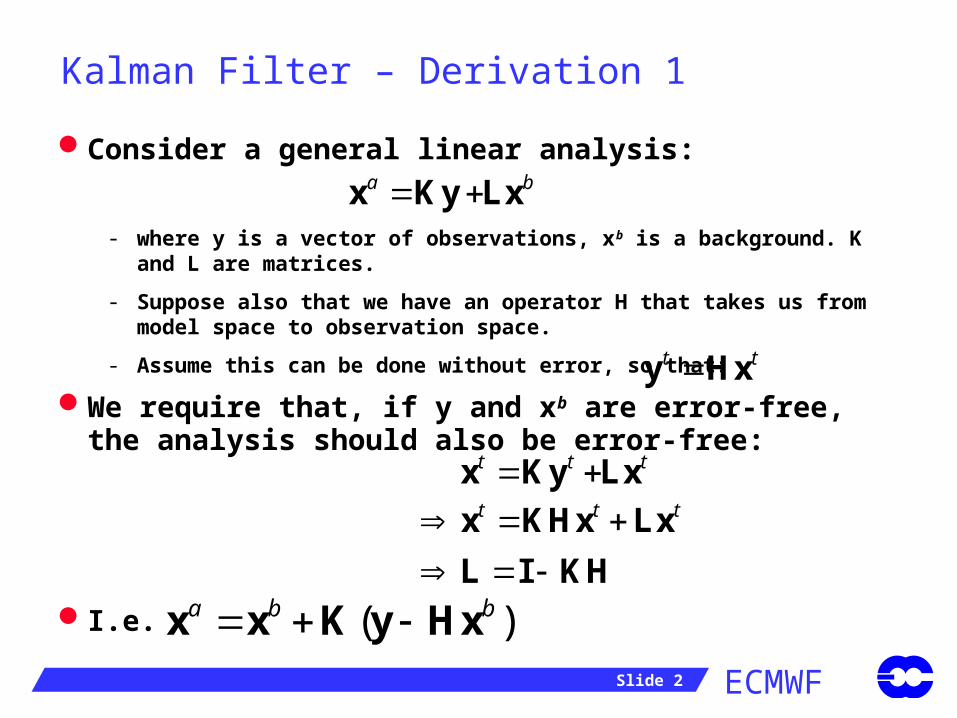
Kalman Filter – Derivation 1
Consider any analysis of the form:
Define errors,
Then:
- Where is representativeness error.
- ( is often ignored.)
Assume that the errors are unbiased.
a b b x x K y Hx
r t t ε y Hx
, , etc.b b t o t ε x x ε y y
a b o r b
o r b
ε ε K ε ε Hε
K ε ε I KH ε
rε
ECMWF Slide 4
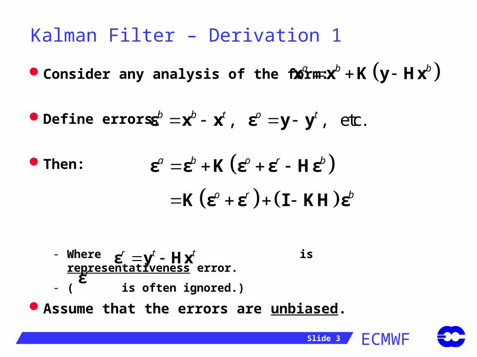
Kalman Filter – Derivation 1
Assume that is uncorrelated with
The covariance matrix for the analysis error is:
o rε ε
a b o r b
o r b
ε ε K ε ε Hε
K ε ε I KH ε
bε
T
T T T
T T
a a a
o r o r b
b b b
P ε ε
K ε ε ε ε HP H K
KHP P H K P
ECMWF Slide 5
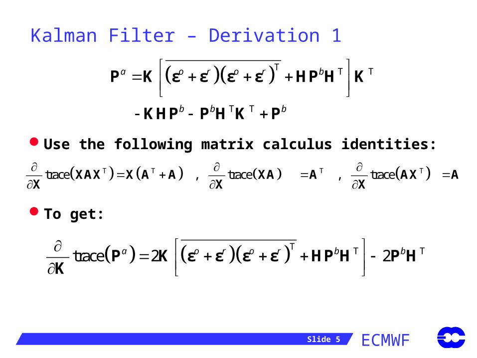
Kalman Filter – Derivation 1
Use the following matrix calculus identities:
To get:
T T T
T T
a o r o r b
b b b
P K ε ε ε ε HP H K
KHP P H K P
T T T Ttrace , trace , trace
XAX X A A XA A AX AX X X
T T Ttrace 2 2a o r o r b b P K ε ε ε ε HP H P H
K
ECMWF Slide 6
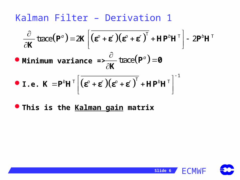
Kalman Filter – Derivation 1
Minimum variance =>
I.e.
This is the Kalman gain matrix
T T Ttrace 2 2a o r o r b b P K ε ε ε ε HP H P H
K
trace a
P 0
K
1
TT Tb o r o r b
K P H ε ε ε ε HP H
ECMWF Slide 7
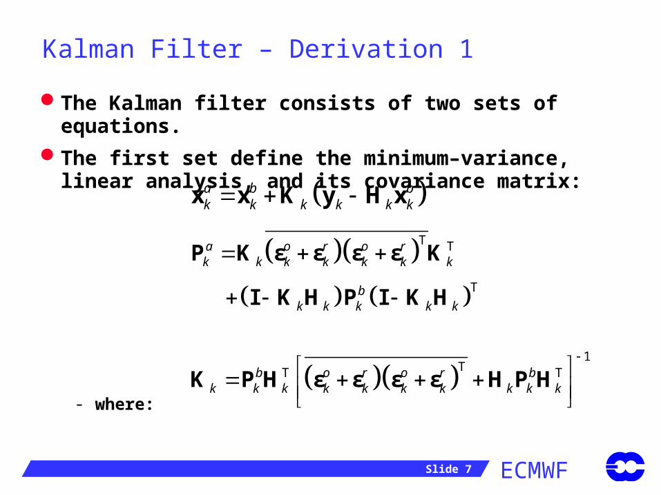
Kalman Filter – Derivation 1
The Kalman filter consists of two sets of equations.
The first set define the minimum–variance, linear analysis, and its covariance matrix:
- where:
a b bk k k k k k x x K y H x
1
TT Tb o r o r bk k k k k k k k k k
K P H ε ε ε ε H P H
T T
T
a o r o rk k k k k k k
bk k k k k
P K ε ε ε ε K
I K H P I K H
ECMWF Slide 8
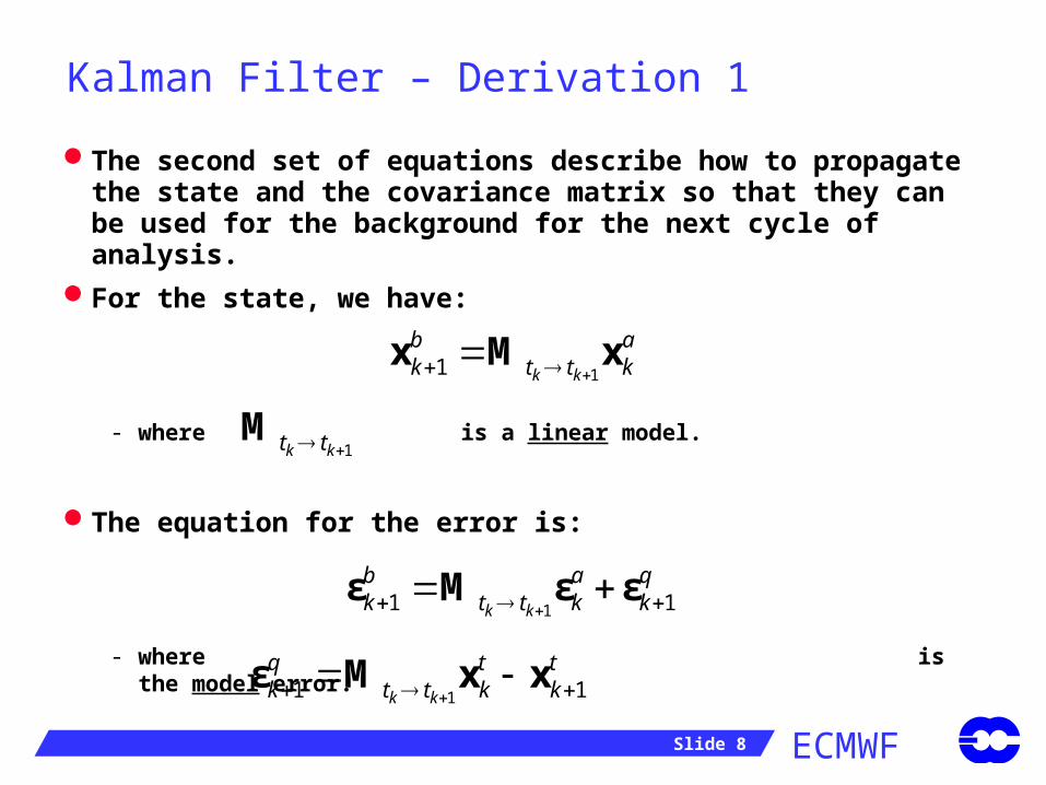
Kalman Filter – Derivation 1
The second set of equations describe how to propagate the state and the covariance matrix so that they can be used for the background for the next cycle of analysis.
For the state, we have:
- where is a linear model.
The equation for the error is:
- where is the model error.
11 k k
b ak t t k x M x
1k kt t M
11 1k k
b a qk t t k k ε M ε ε
11 1k k
q t tk t t k k ε M x x
ECMWF Slide 9
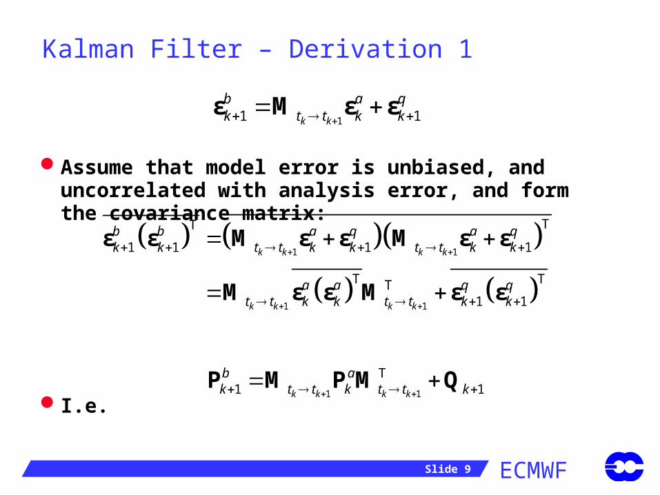
Kalman Filter – Derivation 1
Assume that model error is unbiased, and uncorrelated with analysis error, and form the covariance matrix:
I.e.
11 1k k
b a qk t t k k ε M ε ε
1 1
1 1
TT
1 1 1 1
T TT1 1
k k k k
k k k k
b b a q a qk k t t k k t t k k
a a q qt t k k t t k k
ε ε M ε ε M ε ε
M ε ε M ε ε
1 1
T1 1k k k k
b ak t t k t t k P M P M Q
ECMWF Slide 10
Kalman Filter – Derivation 1
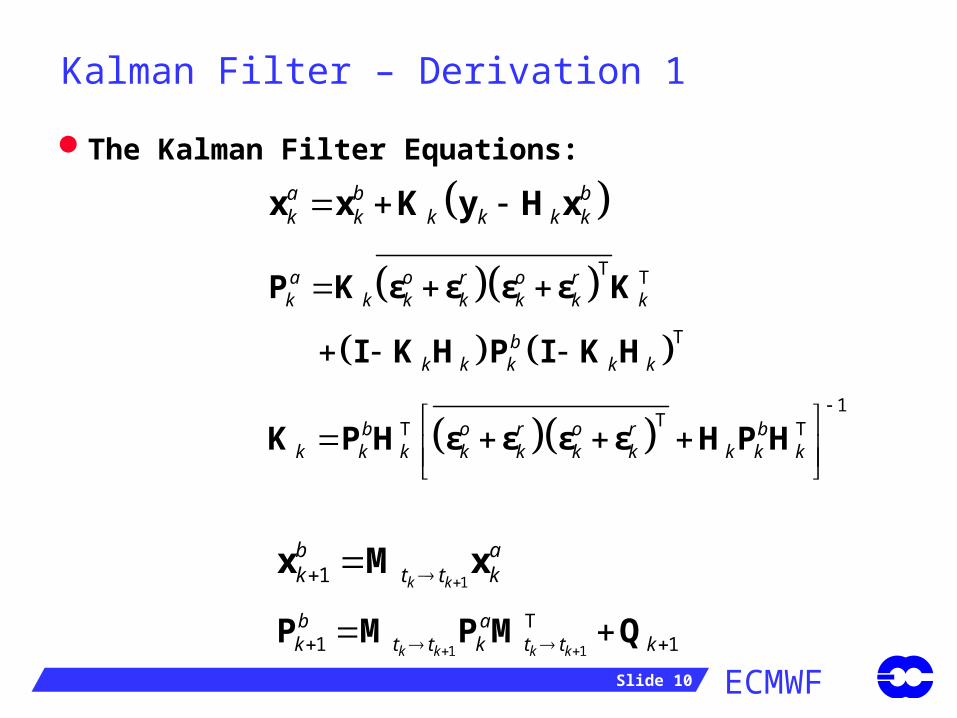
The Kalman Filter Equations:
1 1
T1 1k k k k
b ak t t k t t k P M P M Q
11 k k
b ak t t k x M x
a b bk k k k k k x x K y H x
1
TT Tb o r o r bk k k k k k k k k k
K P H ε ε ε ε H P H
T T
T
a o r o rk k k k k k k
bk k k k k
P K ε ε ε ε K
I K H P I K H
ECMWF Slide 11
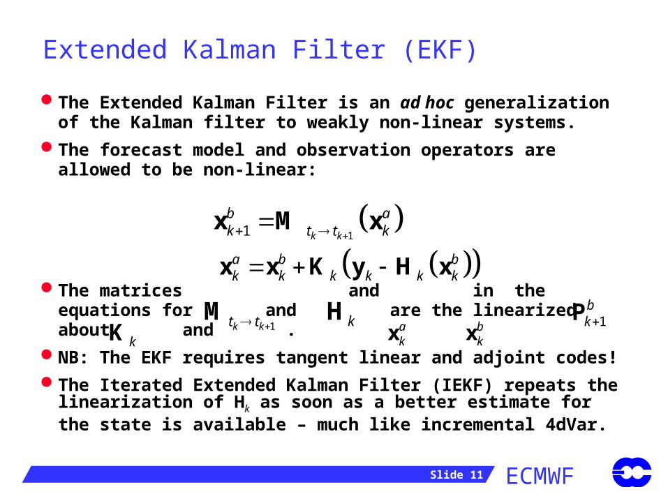
Extended Kalman Filter (EKF)
The Extended Kalman Filter is an ad hoc generalization of the Kalman filter to weakly non-linear systems.
The forecast model and observation operators are allowed to be non-linear:
The matrices and in the equations for and are the linearized about and .
NB: The EKF requires tangent linear and adjoint codes!
The Iterated Extended Kalman Filter (IEKF) repeats the linearization of Hk as soon as a better estimate for the state is available – much like incremental 4dVar.
11 k k
b ak t t k x xM
a b bk k k k k k x x K y xH
1k kt t M kH 1bkP
kK bkxa
kx
ECMWF Slide 12
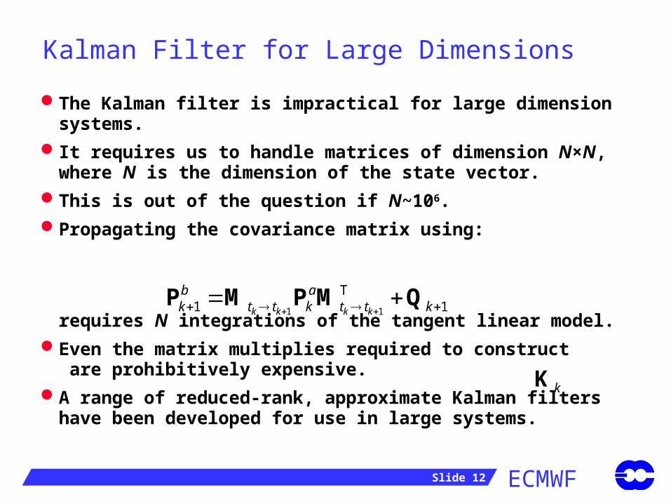
Kalman Filter for Large Dimensions
The Kalman filter is impractical for large dimension systems.
It requires us to handle matrices of dimension N×N, where N is the dimension of the state vector.
This is out of the question if N~106.
Propagating the covariance matrix using:
requires N integrations of the tangent linear model.
Even the matrix multiplies required to construct are prohibitively expensive.
A range of reduced-rank, approximate Kalman filters have been developed for use in large systems.
1 1
T1 1k k k k
b ak t t k t t k P M P M Q
kK
ECMWF Slide 13
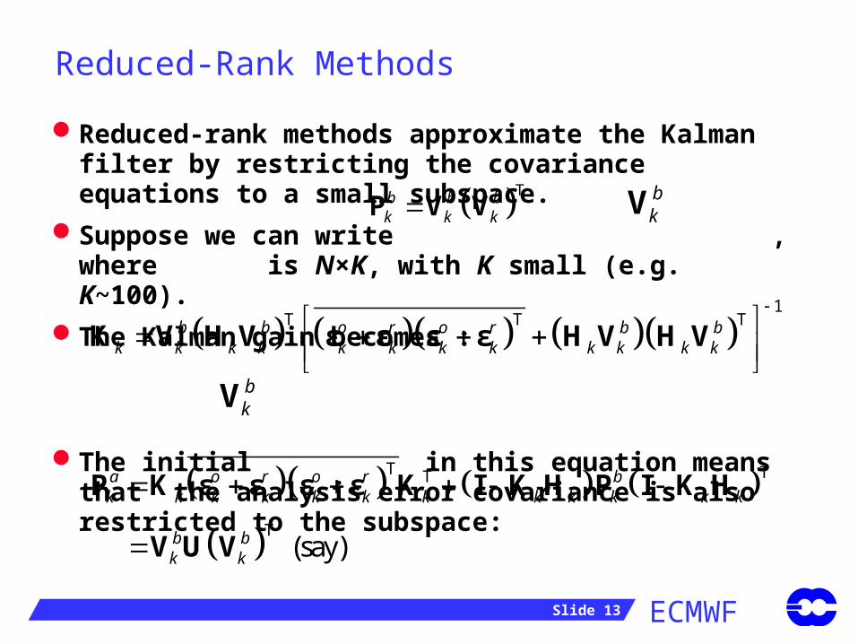
Reduced-Rank Methods
Reduced-rank methods approximate the Kalman filter by restricting the covariance equations to a small subspace.
Suppose we can write , where is N×K, with K small (e.g. K~100).
The Kalman gain becomes :
The initial in this equation means that the analysis error covariance is also restricted to the subspace:
1
T T Tb b o r o r b bk k k k k k k k k k k k
K V H V ε ε ε ε H V H V
Tb b bk k kP V V
bkV
T TT
T (say)
a o r o r bk k k k k k k k k k k k
b bk k
P K ε ε ε ε K I K H P I K H
V U V
bkV
ECMWF Slide 14
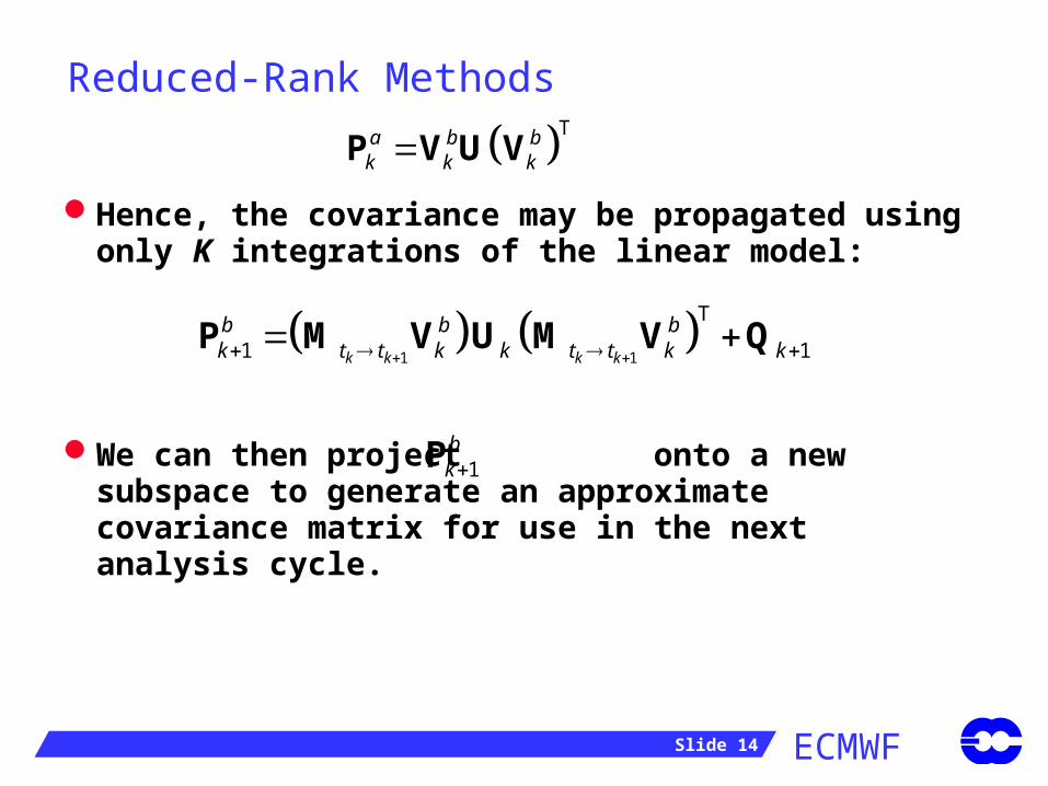
Reduced-Rank Methods
Hence, the covariance may be propagated using only K integrations of the linear model:
We can then project onto a new subspace to generate an approximate covariance matrix for use in the next analysis cycle.
Ta b bk k kP V U V
1 1
T
1 1k k k k
b b bk t t k k t t k k P M V U M V Q
1bkP
ECMWF Slide 15
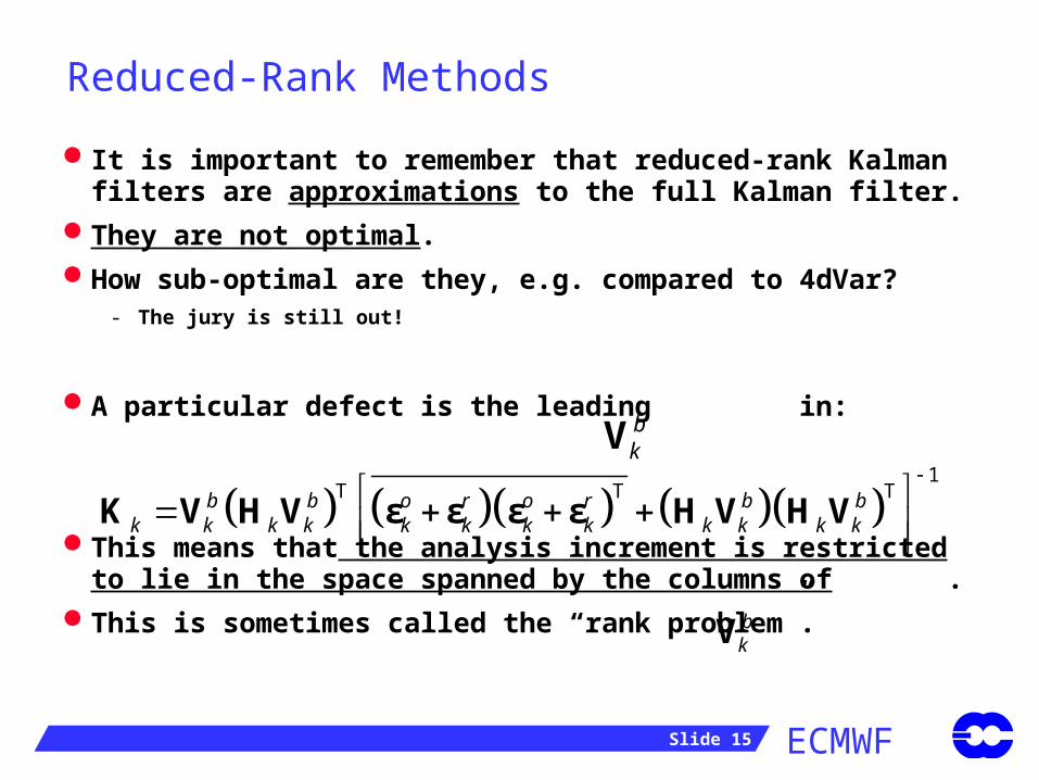
Reduced-Rank Methods
It is important to remember that reduced-rank Kalman filters are approximations to the full Kalman filter.
They are not optimal.
How sub-optimal are they, e.g. compared to 4dVar?- The jury is still out!
A particular defect is the leading in:
This means that the analysis increment is restricted to lie in the space spanned by the columns of .
This is sometimes called the “rank problem”.
1
T T Tb b o r o r b bk k k k k k k k k k k k
K V H V ε ε ε ε H V H V
bkV
bkV
ECMWF Slide 16
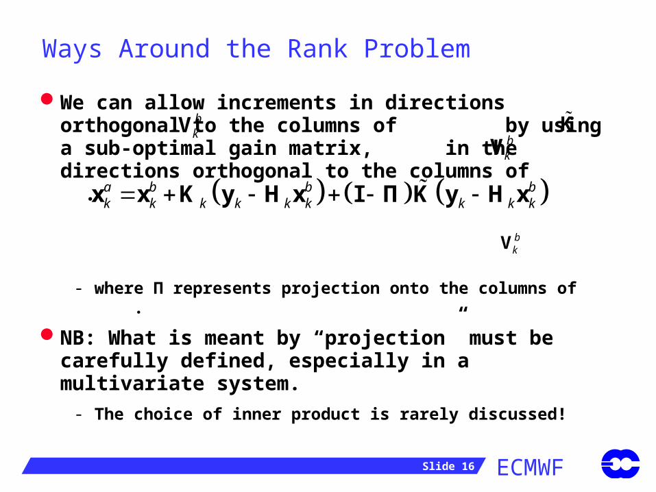
Ways Around the Rank Problem
We can allow increments in directions orthogonal to the columns of by using a sub-optimal gain matrix, in the directions orthogonal to the columns of .
- where Π represents projection onto the columns of .
NB: What is meant by “projection” must be carefully defined, especially in a multivariate system.
- The choice of inner product is rarely discussed!
bkV
bkV
a b b bk k k k k k k k k x x K y H x I Π K y H x
bkV
K
ECMWF Slide 17
Ways Around the Rank Problem
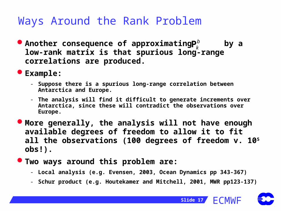
Another consequence of approximating by a low-rank matrix is that spurious long-range correlations are produced.
Example:- Suppose there is a spurious long-range correlation between Antarctica
and Europe.
- The analysis will find it difficult to generate increments over Antarctica, since these will contradict the observations over Europe.
More generally, the analysis will not have enough available degrees of freedom to allow it to fit all the observations (100 degrees of freedom v. 105 obs!).
Two ways around this problem are:- Local analysis (e.g. Evensen, 2003, Ocean Dynamics pp 343-367)
- Schur product (e.g. Houtekamer and Mitchell, 2001, MWR pp123-137)
bkP
ECMWF Slide 18
Ways Around the Rank Problem
Local analysis solves the analysis equations independently for each gridpoint (or for each of a set of regions).
Each analysis uses only observations that are local to the gridpoint (or region).
In this way, the analysis at each gridpoint (or region) is not influenced by distant observations.
The global analysis is no longer a linear combination of the spanning vectors.
The method acts to vastly increase the effective rank of the covariance matrix.
The analysis is sub-optimal because, at each gridpoint, only a subset of available information is used.
ECMWF Slide 19
Ways Around the Rank Problem
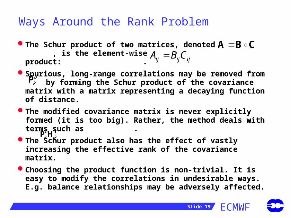
The Schur product of two matrices, denoted , is the element-wise product: .
Spurious, long-range correlations may be removed from by forming the Schur product of the covariance matrix with a matrix representing a decaying function of distance.
The modified covariance matrix is never explicitly formed (it is too big). Rather, the method deals with terms such as .
The Schur product also has the effect of vastly increasing the effective rank of the covariance matrix.
Choosing the product function is non-trivial. It is easy to modify the correlations in undesirable ways. E.g. balance relationships may be adversely affected.
A B Cij ij ijA B C
bkP
Tbk kP H
ECMWF Slide 20
Ensemble Methods
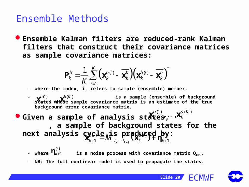
Ensemble Kalman filters are reduced-rank Kalman filters that construct their covariance matrices as sample covariance matrices:
- where the index, i, refers to sample (ensemble) member.
- is a sample (ensemble) of background states whose sample covariance matrix is an estimate of the true background error covariance matrix.
Given a sample of analysis states, , a sample of background states for the next analysis cycle is produced by:
- where is a noise process with covariance matrix Qk+1.
- NB: The full nonlinear model is used to propagate the states.
T( ) ( )
1
1 Kb b i b b i bk k k k k
iK
P x x x x
(1) ( ), ,b b Kk kx x
(1) ( ), ,a a Kk kx x
1
( ) ( ) ( )1 1k k
b i a i ik t t k k x x ηM
( )1ikη
ECMWF Slide 21
Ensemble Methods
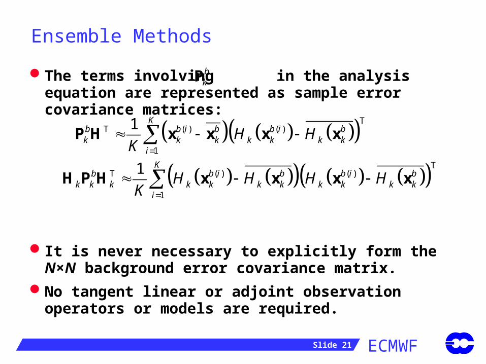
The terms involving in the analysis equation are represented as sample error covariance matrices:
It is never necessary to explicitly form the N×N background error covariance matrix.
No tangent linear or adjoint observation operators or models are required.
bkP
TT ( ) ( )
1
1 Kb b i b b i bk k k k k k k
iK
P H x x x xH H
TT ( ) ( )
1
1 Kb b i b b i b
k k k k k k k k k k kiK
H P H x x x xH H H H
ECMWF Slide 22
Ensemble Methods
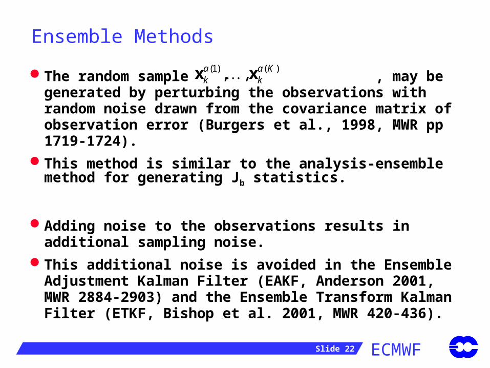
The random sample , may be generated by perturbing the observations with random noise drawn from the covariance matrix of observation error (Burgers et al., 1998, MWR pp 1719-1724).
This method is similar to the analysis-ensemble method for generating Jb statistics.
Adding noise to the observations results in additional sampling noise.
This additional noise is avoided in the Ensemble Adjustment Kalman Filter (EAKF, Anderson 2001, MWR 2884-2903) and the Ensemble Transform Kalman Filter (ETKF, Bishop et al. 2001, MWR 420-436).
(1) ( ), ,a a Kk kx x
ECMWF Slide 23
Ensemble Methods
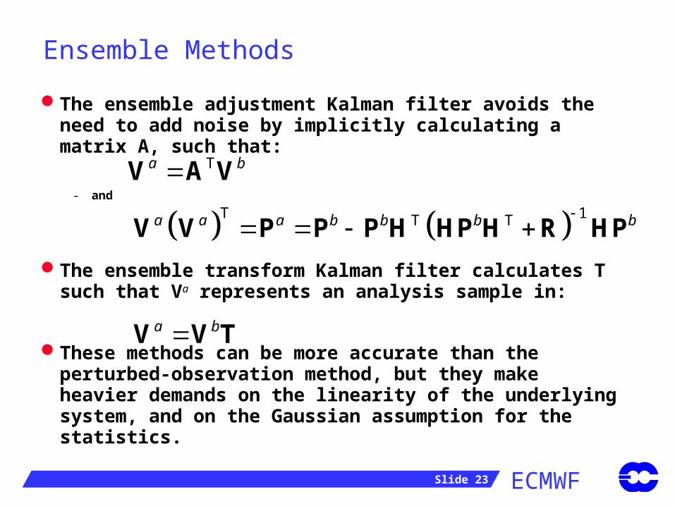
The ensemble adjustment Kalman filter avoids the need to add noise by implicitly calculating a matrix A, such that:
- and
The ensemble transform Kalman filter calculates T such that Va represents an analysis sample in:
These methods can be more accurate than the perturbed-observation method, but they make heavier demands on the linearity of the underlying system, and on the Gaussian assumption for the statistics.
Ta bV A V
a bV V T
T 1T Ta a a b b b b V V P P P H HP H R HP
ECMWF Slide 24
Other Low-Rank Methods
Ensemble methods are popular and attractive because they don’t require adjoint or tangent linear codes. However, a random basis is unlikely to be optimal.
Singular vectors, bred modes, etc. can be used to define deterministic subspaces for reduced-rank Kalman filtering that attempt to capture important aspects of covariance evolution.
ECMWF RRKF (R.I.P.)
- defined a subspace that evolved into the leading eigenvectors of the forecast error covariance matrix at day 2.
SEEK, SEIK, SSEIK, SEPLK (Pham et al, 1998)- a plethora of evolving/partially-evolving subspaces and a plague of acronyms!
Reduced Order Kalman Filter (Farrell and Ioannou, 2001)- uses model-reduction techniques to define an optimal subspace.
ECMWF Slide 25
Non-Gaussian Methods
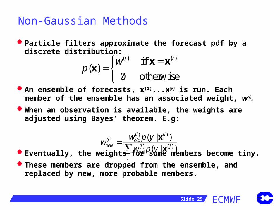
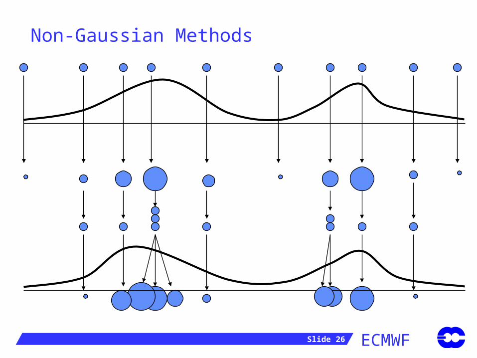
Particle filters approximate the forecast pdf by a discrete distribution:
An ensemble of forecasts, x(1)...x(K) is run. Each member of the ensemble has an associated weight, w(i).
When an observation is available, the weights are adjusted using Bayes’ theorem. E.g:
Eventually, the weights for some members become tiny.
These members are dropped from the ensemble, and replaced by new, more probable members.
( ) ( )if ( )
0 otherwise
i iwp
x xx
( ) ( )( ) oldnew ( ) ( )
old
( | )
( | )
i ii
i j
j
w p yw
w p y
x
x
ECMWF Slide 26
Non-Gaussian Methods
ECMWF Slide 27
Non-Gaussian Methods
Particle filters work well for highly-nonlinear, low-dimensional systems.- Successful applications include missile tracking, computer vision, etc.
(see the book “Sequential Monte Carlo Methods in Practice”, Doucet, de Freitas, Gordon (eds.), 2001)
van Leeuwen (2003) has successfully applied the technique for an ocean model.
The main problem to be overcome is that, for a large-dimensional system, with lots of observations, almost any forecast will contradict an observation somewhere on the globe.- => Every cycle, unless the ensemble is truly enormous, all the particles
(forecasts) are highly unlikely (given the obseravtions).
- van Leeuwen has recently suggested methods that may get around this problem.
ECMWF Slide 28
Non-Gaussian Methods
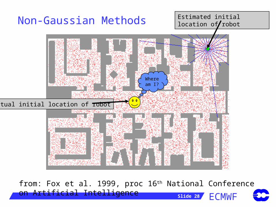
from: Fox et al. 1999, proc 16th National Conference on Artificial Intelligence
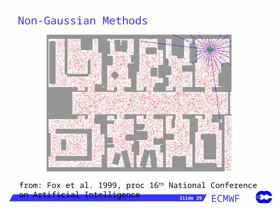
Estimated initial location of robot
Actual initial location of robot
Where am I?
ECMWF Slide 29
Non-Gaussian Methods
from: Fox et al. 1999, proc 16th National Conference on Artificial Intelligence
ECMWF Slide 30
The Non-Sequential Approach
All the preceding is based on the sequential (recursive) view of the filtering problem:
An optimal estimate for step k+1 is produced using only the state and covariance matrices from step k.
All the information from earlier steps is brought to the present step via the covariance matrices.
The advantage of the sequential approach is that we don’t need to go back any further than the previous step in order to determine the current analysis.
The disadvantage is that we must explicitly propagate the covariance matrices.
For very large systems, the matrices are so enormous that a non-sequential approach may be preferable.

ECMWF Slide 31
Kalman filter - Wikipedia dai - Mike Fisher - 7a http://en2.wikipedia.org/wiki/Kalman_filter
1 of 1 12/11/03 12:21
Main Page | Recent changes| Edit this page| Page historyPrintable version
Not logged inLog in | HelpGo Search
Kalman filterFrom Wikipedia, the free encyclopedia.
The Kalman filter (named after its inventor, Rudolf E Kalman ) is an efficient recursive computational solution of the least-squares method, which is applicable to distinguishing signals from noise so as to predict changes in a modeled system with time.
Kalman filtering is used extensive in control systemsengineering.
Compare with: Wiener filter
External links
The Kalman FilterKalman FilteringKalman filters
Edit this page | Discuss this page| Page history| What links here | Related changes
Main Page | About Wikipedia | Recent changes | Go Search
This page was last modified 11:51, 18 Jun 2003. All text is available under the terms of the GNU Free Documentation License.
Main PageRecent changesRandom pageCurrent events
Edit this pageDiscuss this pagePage historyWhat links hereRelated changes
Special pagesBug reportsDonations
ECMWF Slide 32
Equivalence of Kalman Smoother and 4dVar
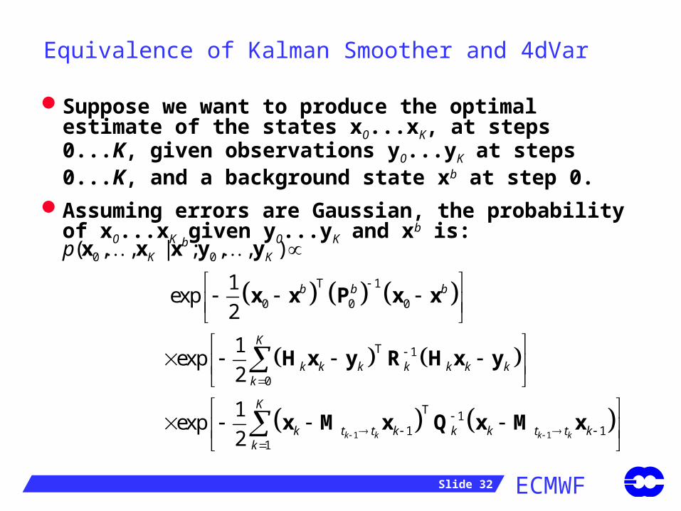
Suppose we want to produce the optimal estimate of the states x0...xK, at steps 0...K, given observations y0...yK at steps 0...K, and a background state xb at step 0.
Assuming errors are Gaussian, the probability of x0...xK given y0...yK and xb is:
1 1
0 0
T 1
0 0 0
T 1
0
T 11 1
1
( , , | ; , , )
1exp
2
1exp
2
1exp
2 k k k k
bK K
b b b
K
k k k k k k kk
K
k t t k k k t t kk
p
x x x y y
x x P x x
H x y R H x y
x M x Q x M x
ECMWF Slide 33
Equivalence of Kalman Smoother and 4dVar
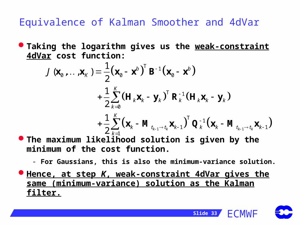
Taking the logarithm gives us the weak-constraint 4dVar cost function:
The maximum likelihood solution is given by the minimum of the cost function.
- For Gaussians, this is also the minimum-variance solution.
Hence, at step K, weak-constraint 4dVar gives the same (minimum-variance) solution as the Kalman filter.
1 1
T 10 0 0
T 1
0
T 11 1
1
1( , , )
21
2
1
2 k k k k
b bK
K
k k k k k k kk
K
k t t k k k t t kk
J
x x x x B x x
H x y R H x y
x M x Q x M x
ECMWF Slide 34
Equivalence of Kalman Smoother and 4D-Var
The solution of the minimization problem differs from the Kalman filter solution at steps 0…K-1.
- The 4dVar solution for step k is optimal with respect to observations at steps 0…K.
- The Kalman filter solution at step k is optimal only with respect to observations at steps 0…k.
I.e. weak constraint 4D-Var is equivalent to the Kalman smoother.
- A purely algebraic proof of this equivalence is given by Ménard and Daley (1996, Tellus 48A, 221-237). (See also Li and Navon (2001) QJRMS, 661-684.)
- This proof shows that the equivalence does not depend on the statistical assumptions made in formulating the analysis problem.
ECMWF Slide 35
The Non-Sequential Approach
So, to determine the optimal state at step K, given observations at steps 0...K, and a background at step 0, we can:
- Either: run a sequential Kalman filter, starting from the background at step 0, and updating the N×N covariance matrices at each step.
- Or: minimize the weak-constraint 4dVar cost function using all observations for steps 0…K.
The sequential approach is impractical for large N.
In principle, the 4dVar approach becomes impractical as K becomes large.
What may save 4dVar is the limited memory of the Kalman filter.- The analysis is insensitive to observations in the distant past
- => We can minimize over steps K-p...K, instead of 0...K.
ECMWF Slide 36
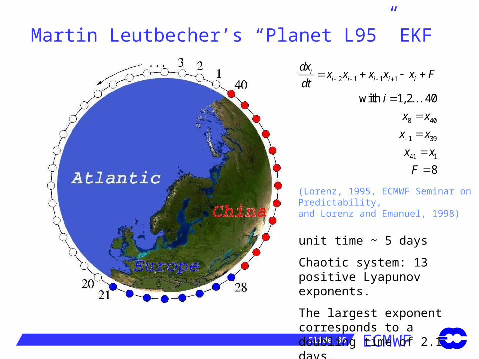
2 1 1 1
0 40
1 39
41 1
with 1,2 40
8
ii i i i i
dxx x x x x F
dti
x x
x x
x x
F
(Lorenz, 1995, ECMWF Seminar onPredictability,and Lorenz and Emanuel, 1998)
unit time ~ 5 days
Chaotic system: 13 positive Lyapunov exponents.
The largest exponent corresponds to a doubling time of 2.1 days.
Martin Leutbecher’s “Planet L95” EKF
ECMWF Slide 37
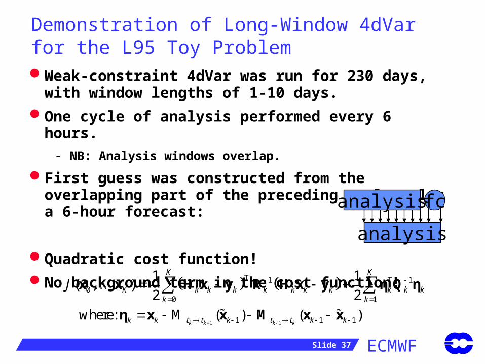
Demonstration of Long-Window 4dVar for the L95 Toy ProblemWeak-constraint 4dVar was run for 230 days, with
window lengths of 1-10 days.
One cycle of analysis performed every 6 hours.
- NB: Analysis windows overlap.
First guess was constructed from the overlapping part of the preceding cycle, plus a 6-hour forecast:
Quadratic cost function!
No background term in the cost function!
analysis fc
analysis
1 1
T 1 T 10
0 1
1 1 1
1 1( , , )
2 2
where: ( ) ( )k k k k
K K
K k k k k k k k k k kk k
k k t t k t t k k
J
x x H x y R H x y η Q η
η x x M x x
M
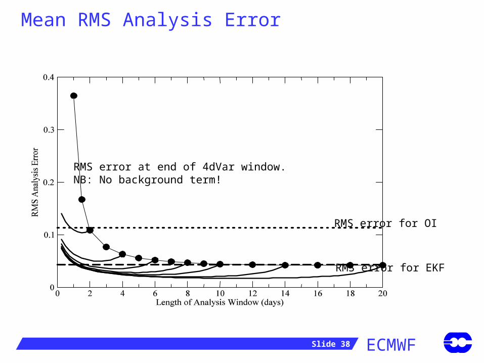
ECMWF Slide 38
RMS error for EKF
Mean RMS Analysis Error
RMS error for OI
RMS error at end of 4dVar window.NB: No background term!
ECMWF Slide 39
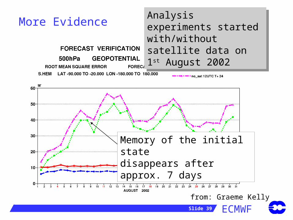
More Evidence Analysis experiments started with/without satellite data on 1st August 2002
Analysis experiments started with/without satellite data on 1st August 2002
from: Graeme Kelly
Memory of the initial statedisappears after approx. 7 days
ECMWF Slide 40
0 1 2 3 4 5 6 7 8 9 10 1112 13 14 15 16 17 1819 20 2122 23 24 2526 27 28 29 30Time (days)
0
2
4
6
8
10
12
14
16
18
20
RM
S sp
read
of
500h
Pa h
eigh
t (m
)Analysis EnsembleMore Evidence
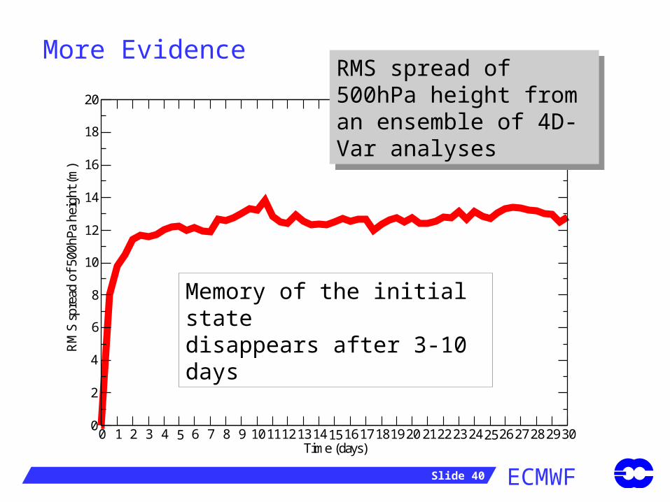
RMS spread of 500hPa height from an ensemble of 4D-Var analyses
RMS spread of 500hPa height from an ensemble of 4D-Var analyses
Memory of the initial statedisappears after 3-10 days
ECMWF Slide 41
0 1 2 3 4 5 6 7 8 9 10 1112 13 14 15 16 17 1819 20 2122 23 24 2526 27 28 29 30Time (days)
0
0.0001
0.0002
0.0003
0.0004
RM
S sp
read
of
leve
l 49
(~85
0hPa
) sp
ecif
ic h
umid
ity
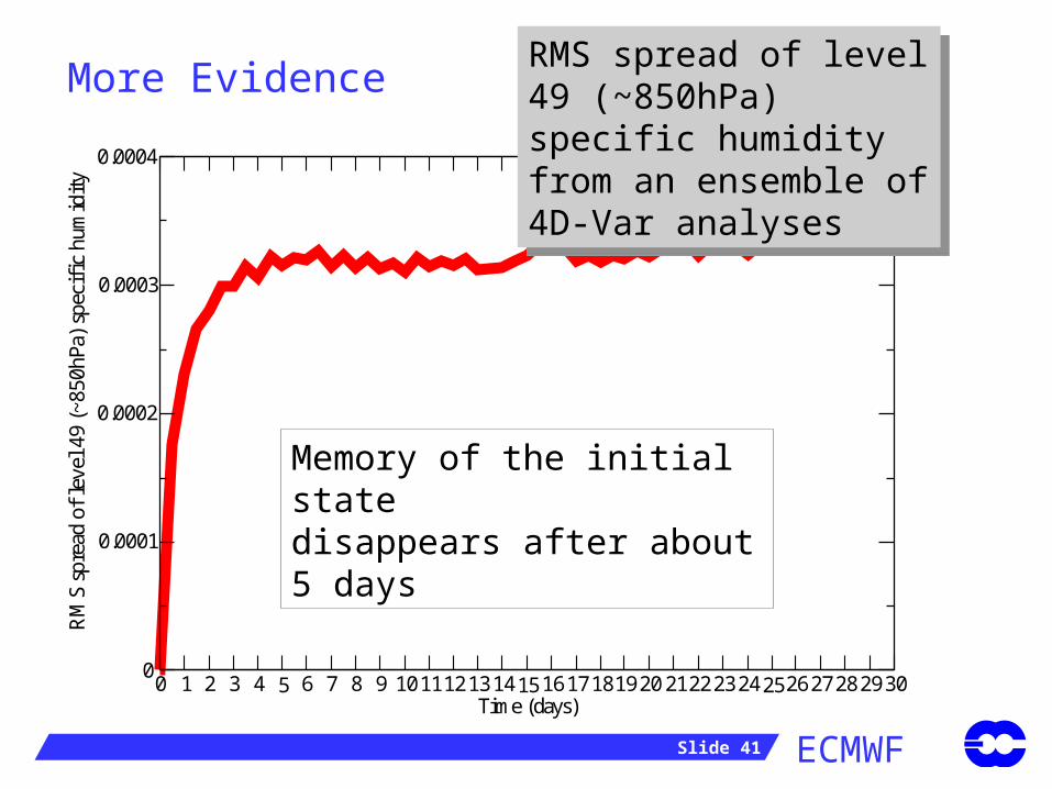
Analysis EnsembleMore Evidence RMS spread of level 49 (~850hPa) specific humidity from an ensemble of 4D-Var analyses
RMS spread of level 49 (~850hPa) specific humidity from an ensemble of 4D-Var analyses
Memory of the initial statedisappears after about 5 days
ECMWF Slide 42
Long-Window, Weak-Constraint 4dVar
Long window, weak constraint 4dVar is equivalent to the Kalman filter, provided we make the window long enough.
For NWP, 3-10 days is long enough.
This makes long-window, weak constraint 4dVar expensive.
But, the resulting Kalman filter is full-rank.
ECMWF Slide 43
Summary
The Kalman filter is the optimal (minimum-variance) analysis for a linear system.
For weakly nonlinear systems, the extended Kalman filter can be used, but it needs adjoints and tangent linear models and observation operators.
Ensemble methods are relatively easy to develop (no adjoints required), but little rigorous investigation of how well they approximate a full-rank Kalman filter has been carried out.
Particle filters are interesting, but it is not clear how useful they are for large-dimension systems.
For large systems, the covariance matrices are too big to be handled.
- We must either use low-rank approximations of the matrices (and risk destroying the advantages of the Kalman filter)
- Or use the non-sequential approach (weak-constraint 4dVar).