Embed Size (px)
Citation preview
POLITECNICO DI MILANO
Ph.D. in Hydraulics Engineering
XXIII Course
ECOHYDROLOGICAL MODELLING OF SOIL WATER AND NUNTRIENTS DYNAMICS IN TROPICAL AND SUBTROPICAL BIOMES
Tutor: Prof. Carlo DE MICHELE
Supervisor: Prof. Carlo DE MICHELE
Ph.D. Course Coordinator: Prof. Alberto GUADAGNINI
Ph.D. Dissertation of
Davide DONZELLI
Milano, January 2012

III
Sommario
Il presente lavoro descrive un approccio eco-idrologico allo studio delle interazioni tra cicli idrologici
e biogeochimici in biomi tropical e sub-tropicali, determinati dalla disponibilità di risorse nel suolo e
dalla competizione tra le componenti erbacee e arboree-arbustive che dominano tali ecosistemi.
Un primo modello si focalizza sulla competizione per acqua e azoto minerale tra tali componenti,
rappresentate attraverso un sistema dinamico non lineare, che viene studiato attraverso l’analisi di
biforcazione con continuazione numerica, sotto due ipotesi opposte di status competitivo, entrambe
supportate in letteratura. Il comportamento del modello viene utilizzato per discriminare le due ipotesi
attraverso un test statistico su un dataset di misurazioni compiute in differenti savane in Africa.
Il modello viene inoltre confrontato con i risultati di simulazioni ottenute tramite un modello
biogeochimico a scala globale, e sono studiate le variazioni di produttività primaria lungo gradienti di
disponibilità di queste due risorse.
Un secondo modello introduce la dinamica del fosforo nel suolo, studiando le condizioni di
limitazione e co-limitazione di N e P nello stesso intervallo latitudinale. Vengono descritte la
dinamica dell’acqua nel suolo e l’influenza delle condizioni di umidità sui processi di
mineralizzazione delle componenti organiche di questi due nutrienti. Il comportamento del modello
viene confrontato con risultati ottenuti da studi di fertilizzazione a scala regionale.
IV
Abstract
The present work describes an eco-hydrological approach in order to analyze the interaction between
hydrological and biogeochemical cycles in tropical and sub-tropical biomes, seen as ecosystems
shaped by resources limitation and competitition between the two dominating plant functional types of
trees and grasses.
A first model investigates the tree-grass competition for multiple resources, representing the
characteristics biomes succession mainly as the results of the dynamical behavior of tree and grasses
competing for water and mineral in a shared volume of soil.
We use a simple dynamical resource-competition model considering two contrasting hypotheses about
the behavior of tree and grasses respect to the resources: 1) tree is the superior competitor for nitrogen
and grass is the superior competitor for water, and 2) tree is the superior competitor for water, and
grass for nitrogen.
We study the model’s properties in both the two different hypotheses, calculating steady states and
bifurcations. We use data of some african savanna and a statistical analysis to select the hypothesis
which better represent the data.
In addition we compare the model’s results with a global simulated database finding an agreement of
about 72%. Finally we study patterns of vegetation along two gradients of resources in order to
investigate the potential changes of vegetation under climate variability, and patchiness of soil
properties.
We develop a second model which focuses on nitrogen and phosporous limitation in the same
latitudinal range. We start from a minimal description of the dynamics of soil moisture and its
interaction with the cycling of nutrients in soil, and in particular with the mineralization-
immobilization turnover. We shows that, despite its parsimonius parameterization, this model is able
to capture relevant characteristics of the observed patterns of nutrient limitation, in particular those
obtained in nutrient enrichment experiments.
V
Contents
SOMMARIO ....................................................................................................................................... III
ABSTRACT ......................................................................................................................................... IV
CONTENTS ....................................................................................................................................... V
LIST OF FIGURES ............................................................................................................................ VI
1 INTRODUCTION ........................................................................................................................... 9
1.1 OPEN PROBLEMS IN SAVANNAS DYNAMICS: AN OVERVIEW ...................................................... 10 1.2 PLANT-WATER RELATIONS IN TROPICAL AND SUBTROPICAL BIOMES ........................................ 13 1.3 NUTRIENTS DYNAMICS AND PATTERNS OF RESOURCE LIMITATION ........................................... 16
2 NUMERICAL TECHNIQUES FOR DYNAMICAL SYSTEMS ............................................ 23
2.1 CONTINUATION METHODS FOR BIFURCATION ANALYSIS ........................................................... 24 2.1.1 Continuation methods in MATCONT ................................................................................ 26
2.2 SIMULATION METHODS FOR NON-SMOOTH DYNAMICAL SYTEMS .............................................. 31
3 MODELS DESCRIPTION AND ANALYSIS ............................................................................ 35
3.1 TGSN MODEL: INTRODUCTION AND BIFURCATION ANALYSIS .................................................. 36 3.2 SNPV MODEL: INTRODUCTION AND PARAMETER ESTIMATION ................................................. 44
4 DATA COMPARISON AND RESULTS .................................................................................... 49
4.1 TGSN MODEL: TESTING COMPETITION STATUS HYPOTHESES ................................................... 50 4.2 TGSN MODEL: VALIDATION THROUGH A GLOBAL DATASET ..................................................... 54 4.3 TGSN MODEL: VEGETATION DYNAMICS UNDER GRADIENTS OF RESOURCE AVAILABILITY ...... 59 4.4 SNPV MODEL: ANALYSIS OF GLOBAL PATTERNS OF NUTRIENT LIMITATION ............................. 62
5 CONLUSIONS AND FURTHER DEVELOPMENTS ............................................................. 66
5.1 INSIGHTS FROM TGSN AND SNPV MODEL ............................................................................... 67 5.2 ONGOING ACTIVITIES ................................................................................................................ 68
REFERENCES ..................................................................................................................................... 70
VI
List of figures
FIG. 1.1 DIAGRAM OF BIOME DISTRIBUTION ACCORDING TO MEAN ANNUAL PRECIPITATION AND
TEMPERATURE, FROM WHITTAKER (1975), MODIFIED IN RICKLEFS (2000). THE SUBTROPICAL
CATENA OCCUPIES THE RANGE OF 20°-30° OF AVERAGE TEMPERATURE AND THE FULL RANGE OF
AVERAGE PRECIPITATION. ............................................................................................................. 13 FIG. 1.2 A COLUMN OF SOIL WITH RELATIVE WATER FLUXES, FROM DE MICHELE ET AL. (2008). ......... 15 FIG. 1.3 REPRESENTATION OF THE NITROGEN CYCLE IN SOILS. .............................................................. 17 FIG. 1.4 NITROGEN POOLS (GN/M2) AND FLUXES (GN/M2/YR) AT NYLSVELEY. ..................................... 19 FIG. 1.5 REPRESENTATION OF THE PHOSPOROUS CYCLE IN SOILS. ......................................................... 20 FIG. 1.6 PHOSPOROUS POOLS (GP/M2) AND FLUXES (GP/M2/YR) AT NYLSVELEY. .................................. 21 FIG. 1.7 EFFECT OF NUTRIENTS ENRICHMENT TREATMENTS ON TERRESTIAL BIOMES PRODUCTIVITY. THE
RESULTS ARE EXPRESSED IN TERM OF THE LOGARITHM OF THE RATIO BETWEEN THE MESURED
BIOMASS AFTER THE SPECIFIC TREATMENTS AND THE BIOMASS OF THE CONTROL PLOT. FROM
ELSER ET AL 2007. ........................................................................................................................ 22 FIG. 2.1 THE GRAPH OF ADJACENCY FOR EQUILIBRIUM AND LIMIT CYCLE BIFURCATIONS IN MATCONT.
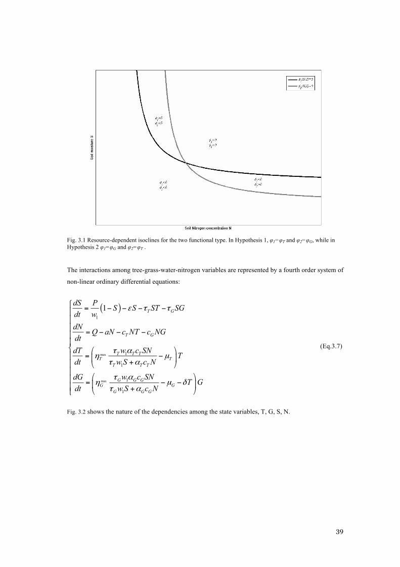
...................................................................................................................................................... 26 FIG. 2.2 MOORE-PENROSE CONTINUATION. .......................................................................................... 30 FIG. 2.3 ILLUSTRATING SCHEMATICALLY TRAJECTORIES OF A PIECEWISE-SMOOTH FLOW. ................... 32 FIG. 3.1 RESOURCE-DEPENDENT ISOCLINES FOR THE TWO FUNCTIONAL TYPE. IN HYPOTHESIS 1, Φ1=ΦT
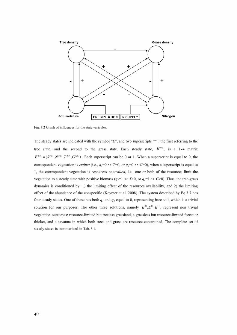
AND Φ2=ΦG, WHILE IN HYPOTHESIS 2 Φ1=ΦG AND Φ2=ΦT . ............................................................ 39 FIG. 3.2 GRAPH OF INFLUENCES FOR THE STATE VARIABLES. ................................................................ 40 FIG. 3.3 BIFURCATION DIAGRAM OF EQ.3.7 IN THE PLANE P-Q AND NORMALIZED TREE ABUNDANCE
WITHIN THE SAVANNA DOMAIN UNDER HYPOTHESIS 1. THE VALUES OF THE FIXED PARAMETERS
ARE: W1=0.35; Ε=1.2; Τ1=3.6; Τ2=25.0; A=0.1; C1=0.3; C2=10.0; Η1=1.8; Η2=3.2; Α1=5.0;
Α2=0.05; Μ1=0.3; Μ2=1.35; Δ=0.115. ........................................................................................... 42 FIG. 3.4 BIFURCATION DIAGRAM OF EQ.3.7 IN THE PLANE P-Q AND NORMALIZED TREE ABUNDANCE
WITHIN THE SAVANNA DOMAIN UNDER HYPOTHESIS 2. THE VALUES OF THE FIXED PARAMETERS
ARE: W1=0.35; Ε=1.2;Τ1=25.0; Τ2=3.6; A=0.1; C1=12.0; C2=0.3; Η1=1.5; Η2=2.5; Α1=0.05;
Α2=5.0; Μ1=2.9; Μ2=0.9; Δ=2.1. ................................................................................................... 43
VII
FIG. 3.5 SIMULATED AND MEASURED VALUES OF NORMALIZED VEGETATION DENSITY AFTER
PARAMETER ESTIMATION. .............................................................................................................. 46 FIG. 3.6 SENSITIVITY ANALYSIS FOR THE PARAMETER ESTIMATED ACCORDING TO SITE SPECIFIC MASS
BALANCES AT NYLSVLEY. ............................................................................................................. 48 FIG. 4.1 SAMPLE ESTIMATES (DOTS) OF KENDALL’S Τ IN VERTICAL (TOP LINE) AND HORIZONTAL
(BOTTOM LINE) SECTIONS, GROUPED FOR SOIL TYPE. THE BOX-AND-WHISKERS PLOTS REPRESENTS
THE SAMPLE DISTRIBUTIONS OF KENDALL’S Τ UNDER THE HYPOTHESIS OF NULL ASSOCIATION
(H0). ............................................................................................................................................. 52 FIG. 4.2 GEOGRAPHICAL DISTRIBUTION OF THE SITES CONSIDERED IN THE GLOBAL DATASET. .............. 55 FIG. 4.3 COMPARISON BETWEEN MODEL’S PREDICTIONS AND THE GLOBAL DATASET IN THE P-Q
BIFURCATION DIAGRAM. GRASSLAND (YELLOW DOTS), SAVANNA (GREEN DOTS), FOREST (BLUE
DOTS) POINTS, AND THE RELATIVE 60% CONVEX HULLS (YELLOW, GREEN, BLUE LINES). .............. 58 FIG. 4.4 COMPARISON BETWEEN THE P-Q BIFURCATION DIAGRAM AND GLOBAL DATASET DIVIDED FOR
CONTINENTS: ASIA AND OCEANIA (LEFT), AFRICA (CENTER), AND AMERICAS (RIGHT). ................ 58 FIG. 4.5 STEADY STATES OF TREE, GRASS, SOIL MOISTURE AND MINERALIZED NITROGEN ALONG THE
PATH P=0.18 Q. PANEL A) SHOWS THE RESOURCE PATH ON THE BIFURCATION DIAGRAM, PANEL B)
GIVES THE EQUILIBRIUM STATES FOR SOIL MOISTURE AND NITROGEN, PANEL C) ILLUSTRATES THE
EQUILIBRIUM STATES FOR TREE AND GRASS. ................................................................................. 60 FIG. 4.6 STEADY STATES OF TREE, GRASS, SOIL MOISTURE AND MINERALIZED NITROGEN ALONG THE
PATH P=0.006 Q. PANEL A) SHOWS THE RESOURCE PATH ON THE BIFURCATION DIAGRAM, PANEL
B) GIVES THE EQUILIBRIUM STATES FOR SOIL MOISTURE AND NITROGEN, PANEL C) ILLUSTRATES
THE EQUILIBRIUM STATES FOR TREE AND GRASS. .......................................................................... 61 FIG. 4.7 DISTRIBUTION OF MAP VALUES UNDER SIMULATED SITES CHARACTERIZED EITHER BY N OR P
LIMITATION. BOXES REPRESENT THE INTER-QUARTILE RANGE, WHISKERS ARE THE MINIMUM AND
MAXIMUM VALUES OBTAINED ....................................................................................................... 63 FIG. 4.8 CONTOUR PLOT OF THE BOUNDARY BETWEEN N AND P LIMITING CONDITIONS FOR DIFFERENT
MAP LEVEL. .................................................................................................................................. 64 FIG. 4.9 THREE-DIMENSIONAL PLOT OF THE BOUNDARY BETWEEN N AND P LIMITING CONDITIONS.
POINTS ARE FORM THE DATASET IN SANKARAN ET AL. (2005). ..................................................... 64 FIG. 4.10 RESULTS FROM SIMULATED 5-YEARS NUTRIENT ENRICHMENT EXPERIMENTS ON THE
SAVANNAS SITE REPORTED IN SANKARAN ET AL. (2005). .............................................................. 65

VIII

9
1 INTRODUCTION
This chapter exposes a review of relevant problems concerning the dynamics of vegetation and its
relation with the hydrological and biogeochemical cycles in tropical and sub-tropical biomes. Both
experimental and theoretical results are reported, focusing in particular on savannas, which represent
one of the most important biomes found within this latitudinal range, and are the most studied from
the prospective of eco-hydrological modelling.
The main results from savannas studies will be presented, focusing on the open problems in this field
of research as well. Then a synthetic description of the main processes in soil involving the
hydrological cycle and the biogeochemical cycles of nitrogen and phosporous.
10
1.1 Open problems in savannas dynamics: an overview
Near-tropical plant communities in which a grassy herbaceous layer coexists with a typically
discontinuous woody stratum cover, broadly called ‘savannas’ (Frost et al. 1986) cover about a fifth of
the global land surface (Scholes and Hall 1994). They occupy those climate regions where the rainfall
is enough to permit tree growth, but there is a sufficiently long dry season that an evergreen closed-
canopy forest does not develop. They are characterized by the frequent occurrence of low-intensity
fires.
Such communities exhibit structural similarities in climatically similar regions of the world,
independent of the vegetation history of those regions (Sankaran et al. 2008), and the mixture is
apparently stable and persistent at large scales, despite high temporal and spatial variability at the
patch scale. The global pattern of tree cover is predictable from environmental variables such as soil
water availability, nutrient supply, fire, and herbivory (Frost et al. 1986; Bucini and Hanan 2007), as
well as considerations on the history of human use. Soil moisture (i.e., the integrated effect of
precipitation and evaporation) and nutrients are the key factors affecting the patterns of primary
production and plant palatability to herbivores in savannas.
Savannas are second only to tropical forests in terms of their contribution to terrestial primary
production (Atjay et al. 1987). In the context of climate change, they represent a substantial terrestial
organic pool, which could act as either a net source or a sink of atmospheric carbon dioxide in future
decades, depending on the path of land use and vegetation-climate feedback that may occurs.
The strong and complex interactions between the woody and herbaceous plants give this biomes a
character of its own. While the central concept – a tropical mixed tree-grass community – is widely
accepted, there is no general consensus on the precise definition of savannas, particularly on the
delimitation of the boundaries.
The upper limit of tree abundance in savannas – expressed in terms of aboveground biomass, basal
area, woody plant cover, or mean height – is constrained by water availability, while actual abundance
at any site is often well below this limit, and is thought to reflect the disturbance history (Scholes et al.
2002, Sankaran et al. 2005).
The savannas of the world all occur in hot region with a highly seasonal rainfall distribution. This
results in a warm dry season (or two, in monsoonal climates) with a duration of three to eight months,
and a hot, wet season for the remainder of the year. The rainfall seasonality occurs as a results of the
latitudinal position of savannas with respect to the main tropical atmospheric circulation systems,
which oscillate north and south across the savanna belt on an annual basis. The near-tropical location
also implies high solar radiation. Since for much of the year there is insufficient water to absorb this
energy by evaporation, it results in high temperature. The high irradiance and heat and the low
11
humidity combine to create a high evaporative demand, which ensures that savannas are in net water
deficit for most of the year, including much of the rainy season.
Previous results (Breman and De Wit 1983; Scholes 1993) have shown that grass production in
drylands, in the absence of trees, increases linearly with mean annual precipitation (a crude measure
of plant available soil moisture) and that the slope of this relation is steeper when the nutrient
availability is high (Vezzoli et al. 2008).
A variety of soils are found under savanna vegetation. This is attributed to the interaction of varied
parent material with weathering regimes of different durations and intensities. The vegetation itself
does not have a profound effect on pedogenesis in savannas, although there is often a close
relationship between soil and vegetation type. Clay illuviation and ion movement are the dominant
soil-forming processes, resulting in distinct soil horizons and catenary sequences. The organic matter
content of savannas soils is generally low. This has been atrributed to the high temperature, which
lead to a high rate of organic matter decomposition, despite the fact that the water deficit in soils
negatively affects this process. It is also due to the frequently sandy nature of savannas soils, and the
predominance of low-activity clays, which do not encourage organic matter stabilisation. These
conditions often provide soils which are deep, structureless and low in plant nutrient.
Nutrient availability, or ‘soil fertility’, is indexed by the clay-plus-silt content of the soil, modified in
some cases by the soil depth, and is thought to be mechanistically tied to the biogeochemical cycles of
nitrogen and phosphorus. As already stated, this provides a further possible link between rainfall and
primary production, since the mineralization process, whereby organically-bound nutrients such as
nitrogen are made available for plant uptake in mineral form, is strongly controlled by soil water
availability (Scholes and Walker 1993; D’Odorico et al. 2003; Botter et al. 2008).
These factors influence in turn the kinds and extent of herbivores, associated animal impacts (Olff et
al. 2002), and the frequency and intensity of fire (D’Odorico et al. 2006, Hanan et al. 2008). In the
presence of trees, the grass production is usually greatly reduced, and the relationship between the
grass production and the woody plant abundance is characteristically non-linear.
Even if some exceptions could occur (for example, Scifres et al. 1982, Teague and Smit 1992, in
which is shown no reduction or even small increase of grass production for low tree density) the most
common pattern is the following: the initial increments in woody abundance sharply reduce the grass
production; but at the point where the woody abundance reaches the climate constraint line (i.e.,
becomes limited by tree-on-tree competition) there is typically still a small component of grass in the
system (Scholes 2003).
There has been many attempts in order to represent the patterns of multiple species co-existence in
terms of competition for multiple resources (Harpole and Tilman 2007, Dybzinski and Tilman 2007,
Higgins et al 2010, Harpole and Suding 2011). The resource ratio theory (Tilman 1982, 1985;
Dybzinski and Tilman 2007) predicts the co-existence of different vegetation species as the result of
multidimensionality niches, e.g., a large number of limiting resources. Using this theory, Harpole and
12
Tilman (2007) have shown how the loss of grassland species is due to the reduction of niche
dimensionality. Dybzinski and Tilman (2007) have investigated experimentally the pair-wise behavior
of six prairie perennial plant species sharing two resources: light and soil nitrogen. Studies in desert
ecosystems (Gebauer and Ehleringer 2000; Gebauer et al. 2002) have shown how the co-presence of
two species of shrubs could be due to the co-limitation of water and nutrients (principally nitrogen).
Competition based models for multiple resources require the determination for each resource of the
superior competitor. In tree-grass competition, a clear evidence of which is the superior competitor for
water and nitrogen seems not to emerge from the literature. The case where tree is the superior
competitor for the nitrogen, and grass is the superior competitor for the water, indicated hereafter as
“Hypothesis 1”, or the converse, denominated “Hypothesis 2”, are both supported by experimental
findings, as well as by explanations based on physiological characteristic of each functional type (tree
or grass) involved. In particular Kraaij and Ward (2006) and Meyer et al. (2009) support Hypothesis 1
while Wang et al. (2010 a, b) support Hypothesis 2.
Such analyses try to identify the superior competitor of each resource using a bottom-up approach, i.e.
through experimental set-ups, too local to produce generalizable evidences, or eco-physiological
principles, that seem to produce questionable ad-hoc explanations.
The first model that will be presented (TGSN) has been developed in order to investigate the tree-
grass competition for two resources, namely soil water and mineral nitrogen, and it will be introduced
in Chapter 3.1. Stationary states are determined and their stability is discussed, focusing the attention
on the domain of tree-grass coexistence (savanna stable state) and considering both Hypothesis 1 and
Hypothesis 2 of competition status.
Successively, data of some african savanna (Sankaran et al. 2005) are compared to the model’s
response through a statistical analysis based on the Kendall’s test of independence in order to support
one of the two hypotheses against the other (or none at all). Once characterized the vegetation
behavior respect to the resources, the model’s predictions are compared to a global simulated dataset,
oputput of a biogeochemical spatially distributed model, applied over all the earth surface.
Two transects along different gradients of precipitation and nitrogen are considered in order to
investigate the potential changes in vegetation structure under climate variability, or changes, and
patchiness of soil properties.
The second model (SNPV) has been developed in order to investigate pattern of resource limitation
(nitrogen and phosphorous) through a minimal model (Chapter 3.2). The paucity of data on P
limitation and the fact that a combined analysis of both nutrients is absent in most terrestrial
biogeochemical modles such as CENTURY (Parton et al. 1987) requires some theoretical effort in
order to address the significance of such interaction. In this model, we neglect resource competition
between different plant functional types, but we address the influence of the hydrological cycle on
nutrient avalability on time scales that are relevant for vegetation dynamics.
13
1.2 Plant-water relations in tropical and subtropical biomes
The strong association between and climates with a hot, wet summer and a warm, dry winter provides
the first clue that water availability is a key factor of the ecology of tropical and subtropical biomes.
The dominance of water availability as a determinant of biomes structure and function is particularly
strong at the dry end of the savanna spectrum, and it has a key role in shaping the peculiar succession
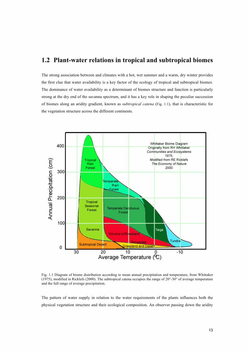
of biomes along an aridity gradient, known as subtropical catena (Fig. 1.1), that is characteristic for
the vegetation structure across the different continents.
Fig. 1.1 Diagram of biome distribution according to mean annual precipitation and temperature, from Whittaker (1975), modified in Ricklefs (2000). The subtropical catena occupies the range of 20°-30° of average temperature and the full range of average precipitation.
The pattern of water supply in relation to the water requirements of the plants influences both the
physical vegetation structure and their ecological composition. An observer passing down the aridity
14
gradient from a moist savanna, receiving perhaps 1000 mm rainfall per year, into a desert shrubland or
grassland receiving 300 mm rainfall per year will be struck by the progressive decrease in the height
and density of the trees, and the consequent change in the proportion of trees to grasses. A similar
change can be noted when passing across variation of soil texture under the same climate and is due,
in part, to the different hydrological characteristics of soils.
The obviousness of the importance of water in savannas can sometimes be a hindrance to
understanding their ecology, since it conceals the importance of other more subtle factors. Water
availability determines savanna function by controlling the duration of the period for which processes
such as primary production and nutrient mineralization can occur. Walter (1971) first noted the
monothonic increasing relationships between annual rainfall and grass production in the dry savannas
of Namibia, and similar relationships have been documented in many parts of the world.
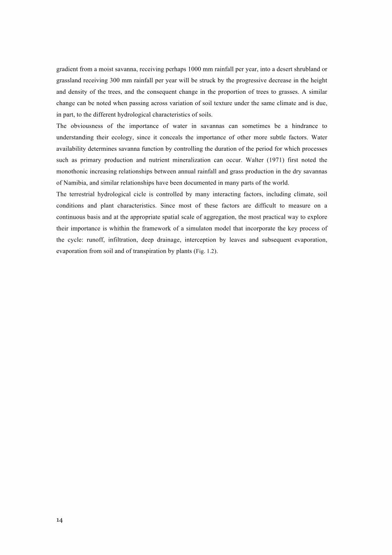
The terrestrial hydrological cicle is controlled by many interacting factors, including climate, soil
conditions and plant characteristics. Since most of these factors are difficult to measure on a
continuous basis and at the appropriate spatial scale of aggregation, the most practical way to explore
their importance is whithin the framework of a simulaton model that incorporate the key process of
the cycle: runoff, infiltration, deep drainage, interception by leaves and subsequent evaporation,
evaporation from soil and of transpiration by plants (Fig. 1.2).
15
Fig. 1.2 A column of soil with relative water fluxes, from De Michele et al. (2008).
In Accatino et al. (2010) it is shown through a simplified hydrological model how the sub-tropical
catena can be interpreted in term of the interaction between soil water competition and vegetation
disturbances like fire.
For 100 ≤ p ≤ 600 mm/y the dry savanna co-existence is permitted by the balanced competition for
limited rainfall and fire influences only the tree-grass ratio. The system would still be a savanna, even
in the absence of fire. For rainfall above 1100 mm/y the moist savanna co-existence can only occur in
the presence of a high level of fire disturbance, because the ecosystem would be a forest in the
absence of fire. In the intermediate range, 600 ≤ p ≤ 1100 mm y-1, savanna is the result of the co-
occurence of water limitation and fire.
The model shows how dry savannas are stable equilibria, while moist savannas are a bi-stable
condition with forest, and it also allows to predict the vegetation structure changes that occur along
gradients of rainfall and fire frequency, and to clarify the distinction between climate-dependent
ecosystems and fire-dependent ecosystems (Bond and Keeley 2005).
16
1.3 Nutrients dynamics and patterns of resource limitation
In this chapter we concentrate on the movement of two key elements – nitrogen and phosphorous –
not as energy carriers, but as building blocks essential for the growth of any organism. It is useful to
examine the pathways of nitrogen and phosphorous against the background of the carbon cycle, since
for the major biological portion of their cycles they are found in organic form (that is, as part of
carbon-based molecules). Among the key processes regulating the passage of N and P through the
ecosystem is the process whereby they are liberated from their carbon bondage, and become available
for uptake by the organisms.
The trademark of systems ecology is a flow diagram consisting of boxes and interconnecting arrows.
The boxes represent reservoir or pools of a particular element, and the arrows show the rate and
direction of transfer (flux) of the element between pools. The fluxes are usually inferred from the rate
of change in the size of their source or sink pools, although some fluxes can be measured through
specific techniques (for example, incubation of soil sample) as we will see in the following.
Identifying and quantifying the fluxes is a considerable improvement beyond a static representation of
the pools sizes, but a complete biogeochemical system analysis requires knowledge of the factors
which control the rate of the flux, as well.
The pathways of carbon, nitrogen and phosphorous are strongly associates, and they form an
interesting continuum from a very open cycle (carbon) to a tightly closed one (phosphorous), with
nitrogen in between. The carbon cycle has large fluxes to and from the atmospheric carbon pool which
is defined as being outside of the system. Therefore, at the scale of a patch of vegetation, the carbon
cycle is ‘open’. The nitrogen cycle also include an atmospheric loop, but it is small relative to the
recycling which occurs within the plant-soil system. Phosphorous cycling is virtually entirely
restricted to the plant-soil system, since atmospheric fluxes are generally neglectible, and it differs
from the nitrogen cycle in the prominence of the inorganic soil pools and the non-biological processes
of exchange between them. The degree of ‘openness’ of the cycle has important consquences on the
potential for loss of elements from the system, and on the rate of recovery after such leakage.
Nitrogen and phosphorous are essential for the growth and functioning of all organisms, and their
availability is a potential constraint on productivity. Since they are required in large quantities relative
to ther elements, they are classified as ‘macronutrients’, being the most frequently limiting nutrients in
terrestrial ecosystems.
Now the two cycles of nitrogen and phosphorous will be described in details. The terrestrial N cycle
comprises soil, plant and animal pools that contain relatively small quantities of biologically active N,
in comparison to the large pools of relatively inert N in the litosphere and atmosphere, but that
nevertheless exert a substancial influence on global biogeochemistry, due to the relatively ‘closeness’
of this cycle in relation. After carbon (ca. 400 g/kg) and oxygen (ca. 450 g/kg)m N is the next most
abundant element in plant dry matter, typically 10-30 g/kg. It is a key component of plant amino and
17
nucleic acids, and chlorophyll, thus directly influencing plant productivity, and is usually acquired by
plants in greater quantity from sil than any other element.
The largest N pool in the plant roopt zone is in the soil organic matter, but this is mostly unavailable
to plants. However, this organic N may be released (mineralised) to form plant-available or mineral N.
Organic matter decomposition is a complex process that occurs, to differing extent, with newly added
plant residues, animal waste products, root exundates and rhizodeposits as well as various existing or
‘native’ soil organic pools. This results in a continuum of organic materials of varying ages, stages of
decay and degree of recalcitrance. Decomposition is mediated largely by soil biota and results
ultimately in release of nutrients in mineral form and loss of c from the soil as CO2 via respiration.The
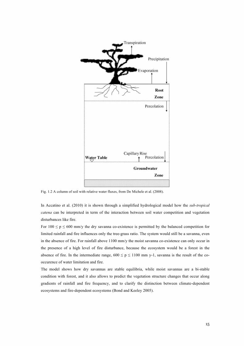
microbial biomass has a pivotal role in the soil N cycle (Fig. 1.3) and was aptly described by Jenkinson
et al. (1990) as “the eye of the needle through wich virtually all nutrient must pass”.
The continuous transfer of mineral N into organic materials via incoporation into soil microbial
biomass, and the subsequent release back into the soluble mineral N pool is known as “mineralization-
immobilization turn-over” or MIT (Jansson and Persson 1982), and it is considered to play a dominant
role in the availability of N for plants in natural ecosystems.
Fig. 1.3 Representation of the nitrogen cycle in soil, from Marschner and Rengel (2007).
Gross N mineralization in soil results in the release of ammonium (NH4+) or ammonia (NH3) by non-
specific heterotrophic soil micro-organism under aerobic and anaerobic conditions. The bulk of N
mineralization occurs in the biologically active surface soil that contains most of the dead and
decomposing litter. The process of gross N immobilization involves microbial assimilation of NH4+
and , to a lesser extent, NO3-.
18
As stated before, it has proved far easier to measure the net effect in soils of MIT, rather than gross
immobilization and mineralization, by simply analysing temporal changes in inorganic N over defined
period, whilst minimising or taking into account losses or gains. The available approaches range from
laboratory incubations to large-scale field studies (Marschner and Rengel 2007).
Ammonium in soil may be oxidised via nitrite (NO2-) to NO3
- at a rate regulated primarily by
availability of NH4+. This process, called nitrification, can be autotrophic or heterotrophic, and from
the relatively small number of microbial species involved, it is greatly influenced by edaphic factors
such as pH, moisture, temperature and aeration.
Plants may acquire N form soil as NH4+, NO3
- or NO2-, and the uptake is an icreasing function of the
respective concentrations in the soil solution, being also influenced by root distribution and soil water
content. The concentration of N in plant dry matter of herabcous plants is typically 10-20 g/kg for
grasses and forbs, and 20-30 g/kg for legumes, due to the effect of micorrhizae symbiosis in fixing
atmospheric nitrogen, and tends to be higher in younger tissues. For woody plants, the concentration
of N varies with plant parts, typically being <5 g/kg for woody tissue and <20 g/kg for leaves, due to
the resorption of available nutrients from dying leaves.
Among the losses that charcterise the N cycle, leaching is the most relevant for its connection with the
hydrological cycle. The two major determinants of this process are the quantity of water passing
through the soil profile and the concentration of soluble elements at that time. Thus leaching occurs
whenever mineral N accumulation in the soil solution coincides with, or is followe by, a period of
high drainage.
Ecosystem disturbances caused by fire, harvest, cultivation and grazing tend to increase the potential
for leaching in both natural and agricultural systems. Reported quantities of mineral N leached vary
enormously within similar ecosystems and even more widely between different ones.
Overall, leaching is exacerbated on light sandy soils, and tend to be much larger in agrosystems that
are frequently disturbed. However, the extent and scale of losses, particularly of the most labile
organic part of the soil N pools, via leaching in natural ecosystems is still relatively unknown and,
despite acknowledgement that these losses may comprise a significant part of the terrestrial N cycle,
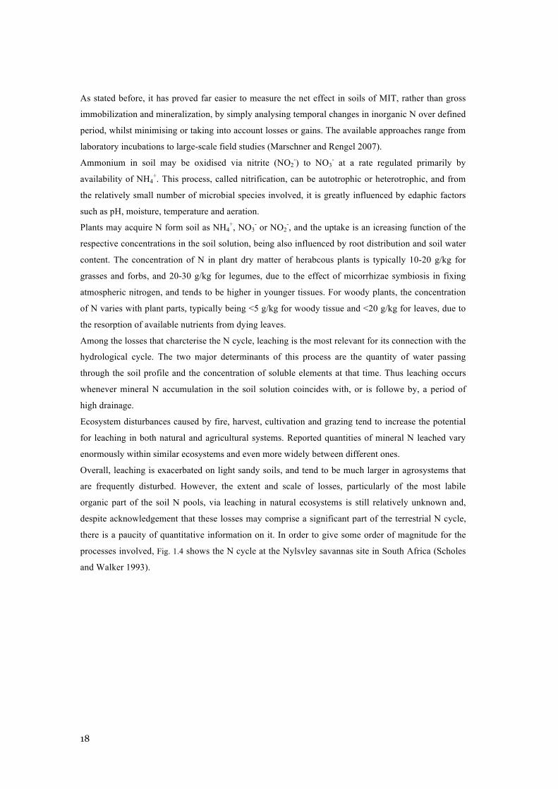
there is a paucity of quantitative information on it. In order to give some order of magnitude for the
processes involved, Fig. 1.4 shows the N cycle at the Nylsvley savannas site in South Africa (Scholes
and Walker 1993).
19
Fig. 1.4 Nitrogen pools (gN/m2) and fluxes (gN/m2/yr) at Nylsveley, from Scholes and Walker (1993).
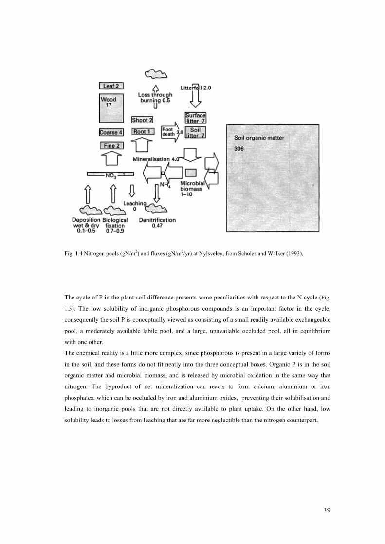
The cycle of P in the plant-soil difference presents some peculiarities with respect to the N cycle (Fig.
1.5). The low solubility of inorganic phosphorous compounds is an important factor in the cycle,
consequently the soil P is conceptually viewed as consisting of a small readily available exchangeable
pool, a moderately available labile pool, and a large, unavailable occluded pool, all in equilibrium
with one other.
The chemical reality is a little more complex, since phosphorous is present in a large variety of forms
in the soil, and these forms do not fit neatly into the three conceptual boxes. Organic P is in the soil
organic matter and microbial biomass, and is released by microbial oxidation in the same way that
nitrogen. The byproduct of net mineralization can reacts to form calcium, aluminium or iron
phosphates, which can be occluded by iron and aluminium oxides, preventing their solubilisation and
leading to inorganic pools that are not directly available to plant uptake. On the other hand, low
solubility leads to losses from leaching that are far more neglectible than the nitrogen counterpart.
20
Fig. 1.5 Representation of the phosporous cycle in soil, from Marschner and Rengel (2007).
Despite sharing an almost equivalent role in limiting the productivity of terrestrial ecosystems, the P
cycle is even less studied in a quantitative way than the N cycle. This is partly due to the impossibility
of using incubation methods to measure the net mineralization of organic P and consequent release of
mineral soluble P by soil biota. In fact, laboratory incubation conditions lead to sorption of the end
phosphate product, preventing the reliability of the measurement of mineral P concentration at the end
of the process and making more difficult the assesment of releases in soils of available P.
Furthermore, the presence of pools of inorganic P that are unavailable to plant complicates the
interpretation of the measurement of total P, since those pools can act as either a source or a sink of
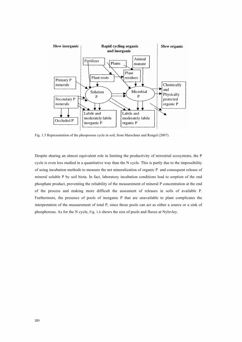
phosphorous. As for the N cycle, Fig. 1.6 shows the size of pools and fluxes at Nylsvley.
21
Fig. 1.6 Phosporous pools (gP/m2) and fluxes (gP/m2/yr) at Nylsveley, from Scholes and Walker (1993).
Past work has highlighted a diverse set of geochemical and ecological factors that can influence the
identity and nature of N and P limitation in particular ecosystems (Vitousek and Howarth 1991). In
terrestrial environments, soil age is a key factor because P becomes increasingly sequestered via
mineralogical transformations occuring over time scales of 103-105 years (Wlaker and Syers 1976,
Vitousek 2004). Thus, tropical ecosystems that were not disturbed by galciation are thought to be
more frequently P-limited because of greater soil age.
On the other hand, regional fire regime can also have a major impact, as fire volatilizes N pools while
leaving P behind (Raison 1979, Hungate et al 2003). This diversity of habitat-specific climatic,
edaphic and ecological influences on N and P availability make it difficult to obtain a broad picture of
their relative importance as limting resource in the biosphere.
Nevertheless, some existing paradigms identify N as the primary limiting nutrient, while recent work
has begun to question this generalization, calling attention to an equivalence of N and P limitation
over a broad set of ecosystems.
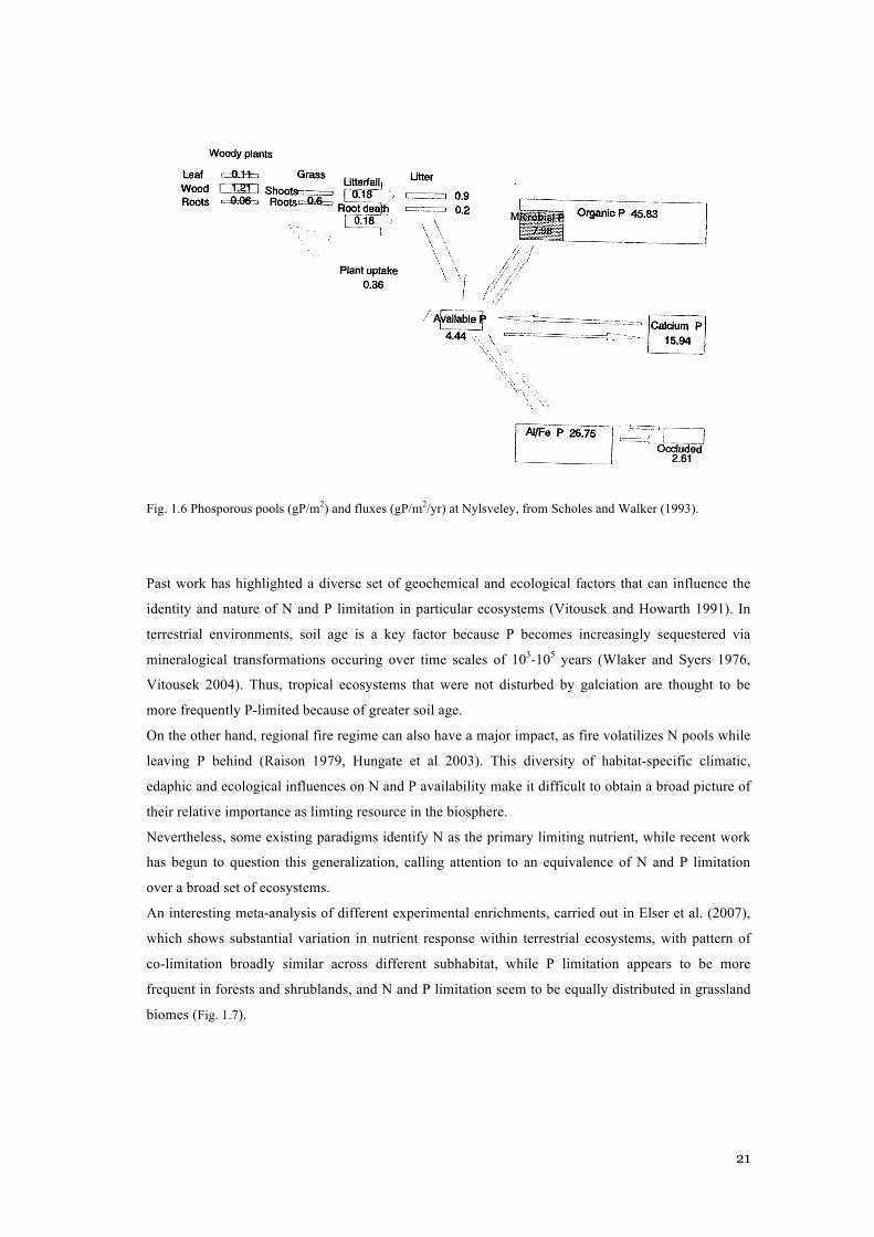
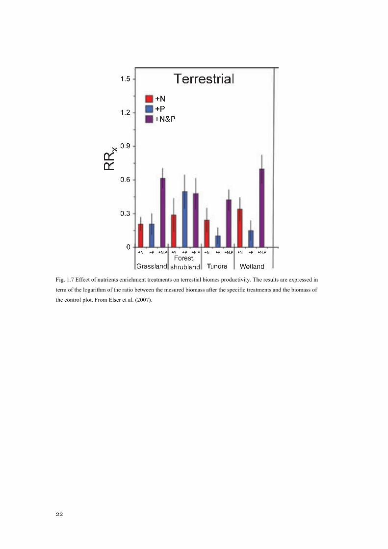
An interesting meta-analysis of different experimental enrichments, carried out in Elser et al. (2007),
which shows substantial variation in nutrient response within terrestrial ecosystems, with pattern of
co-limitation broadly similar across different subhabitat, while P limitation appears to be more
frequent in forests and shrublands, and N and P limitation seem to be equally distributed in grassland
biomes (Fig. 1.7).
22
Figure 2 Relative responses (RRx) of auto-trophs to single enrichment of N or P or tocombined N + P enrichment in varioussubhabitats in terrestrial, freshwater andmarine ecosystems. Data are expressed asin Figure 1.
Table 2 Results of ANOVA!s comparing theeffects of the three nutrient enrichmenttreatments (+N, +P, or +N&P) on auto-troph biomass
System Factor d.f.Sum ofsquares F P-value
All systems Nutrient treatment 2 287.08 217.01 < 0.0001C1: RRNP vs. (RRN and RRP) 1 286.10 432.53 < 0.0001C2: RRN vs. RRP 1 0.99 1.491 0.2222Residuals 2462 1628.5
Terrestrial Nutrient treatment 2 8.121 10.549 < 0.0001C1: RRNP vs. (RRN and RRP) 1 8.121 21.097 < 0.0001C2. RRN vs. RRP 1 <0.001 <0.0001 0.9998Residuals 342
Freshwater Nutrient treatment 2 288.65 232.582 < 0.0001C1: RRNP vs. (RRN and RRP) 1 288.52 464.942 < 0.0001C2: RRN vs. RRP 1 0.14 0.22 0.6375Residuals 1630
Marine Nutrient treatment 2 29.11 16.181 < 0.0001C1: RRNP vs. (RRN and RRP) 1 20.48 22.765 < 0.0001C2: RRN vs. RRP 1 8.63 9.5967 0.0021Residuals 484
The effects of nutrient treatment are also analysed at two orthogonal contrasts: C1. RRNP vs.RRN and RRP and C2. RRN vs. RRP. Results are presented for the pooled data set across allsystems and for each of the three systems analysed separately.
Table 3 Results of a nested ANOVA examin-ing the overall effects on RRX of ecosystemtype (marine, freshwater and terrestrial),nutrient enrichment treatment (+N, +P, or+N&P) and subhabitat (nested within eco-system type; lake benthos, lake pelagic,stream; marine hard-bottom, marine soft-bottom, marine pelagic; grassland ⁄meadow,forest ⁄ shrubland, tundra, wetland)
Factor d.f.Sum ofsquares F P-value
System 2 11.23 9.092 < 0.0001Nutrient treatment 2 286.5 231.9 < 0.0001Subhabitat (system) 8 48.10 9.735 < 0.0001Treatment · system 4 30.88 12.50 < 0.0001Treatment · subhabitat (system) 14 35.66 4.124 < 0.0001Residuals 2434 1503
The effects of nutrient treatment were also analysed at two orthogonal contrasts: (i) N (RRN)vs. P (RRP) addition (P = 0.91) and (ii) either N or P alone (RRN and RRP) vs. both N and P(RRNP) (P < 0.0001).
Letter Ecosystem N and P limitation 5
! 2007 Blackwell Publishing Ltd/CNRS
Fig. 1.7 Effect of nutrients enrichment treatments on terrestial biomes productivity. The results are expressed in
term of the logarithm of the ratio between the mesured biomass after the specific treatments and the biomass of
the control plot. From Elser et al. (2007).

23
2 NUMERICAL TECHNIQUES FOR
DYNAMICAL SYSTEMS
In this chapter will be presented a review of numerical techniques used for the analysis of dynamical
systems. Such techniques will be used for studying the eco-hydrological models presented in the
following chapter. In particular, we are interested in understanding the qualitative behaviour of a
particular system depending on the variations of a small set of free parameters, that is a bifurcation
analysis. We will start in the context of smooth non-linear dynamical systems, for which it exists a
well assessed classification of bifurcation modes, and numerical tools to detect them. Then we will
deal with non-smooth dynamical systems, that represent a rich and active field of research, and an
algorithm for accurate direct numerical simulations of such systems will be presented. This
introduction does not claim to be an exaustive description of these topics, that are subject of still
ongoing researches. Our objective is to introduce the reader in some techniques extensively used for
the analysis of the ecohydrological models which represent the main contribution of this work.
24
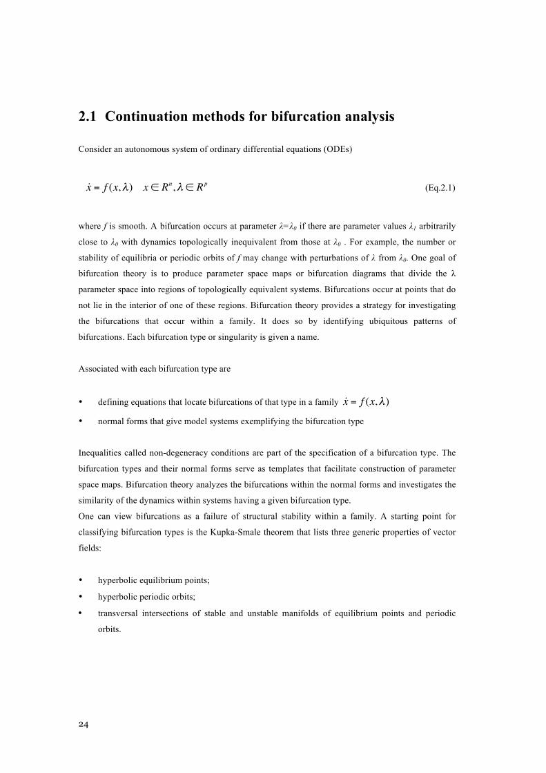
2.1 Continuation methods for bifurcation analysis
Consider an autonomous system of ordinary differential equations (ODEs)
!x = f (x,!) x ! Rn,! ! Rp (Eq.2.1)
where f is smooth. A bifurcation occurs at parameter λ=λ0 if there are parameter values λ1 arbitrarily
close to λ0 with dynamics topologically inequivalent from those at λ0 . For example, the number or
stability of equilibria or periodic orbits of f may change with perturbations of λ from λ0. One goal of
bifurcation theory is to produce parameter space maps or bifurcation diagrams that divide the λ
parameter space into regions of topologically equivalent systems. Bifurcations occur at points that do
not lie in the interior of one of these regions. Bifurcation theory provides a strategy for investigating
the bifurcations that occur within a family. It does so by identifying ubiquitous patterns of
bifurcations. Each bifurcation type or singularity is given a name.
Associated with each bifurcation type are
• defining equations that locate bifurcations of that type in a family !x = f (x,!)
• normal forms that give model systems exemplifying the bifurcation type
Inequalities called non-degeneracy conditions are part of the specification of a bifurcation type. The
bifurcation types and their normal forms serve as templates that facilitate construction of parameter
space maps. Bifurcation theory analyzes the bifurcations within the normal forms and investigates the
similarity of the dynamics within systems having a given bifurcation type.
One can view bifurcations as a failure of structural stability within a family. A starting point for
classifying bifurcation types is the Kupka-Smale theorem that lists three generic properties of vector
fields:
• hyperbolic equilibrium points;
• hyperbolic periodic orbits;
• transversal intersections of stable and unstable manifolds of equilibrium points and periodic
orbits.

25
Different ways that these Kupka-Smale conditions fail lead to different bifurcation types. Bifurcation
theory constructs a layered graph of bifurcation types in which successive layers consist of types
whose defining equations specify more failure modes. These layers can be organized by the
codimension of the bifurcation types, defined as the minimal number of parameters of families in
which that bifurcation type occurs. Equivalently, the codimension is the number of equality conditions
that characterize a bifurcation.
One of the principal uses of bifurcation theory is to analyze the bifurcations that occur in specific
families of dynamical systems. Investigations commonly identify the types of bifurcations in
parameter space maps either by comparison of simulation results with normal forms or by solving
defining equations for those bifurcation types in the systems under investigation and computing
coefficients of the normal forms. Several software packages (AUTO, CONTENT, MATCONT,
XPPAUT, PyDSTool) give implementations of algorithms that perform the latter type of analysis. The
numerical core of these packages consist of
• regular implementations of defining equations for the bifurcation types;
• equation solvers such as Newton's method;
• numerical continuation methods for differential equations;
• computation of normal forms;
• initial and
• boundary value solvers for differential equations.
The continuation methods compute curves of solutions to regular systems of N equations in N+1
variables. The bifurcation analysis of a system implemented to varying degrees in the packages listed
above is based upon the following strategy:
• an initial equilibrium or periodic orbit is located;
• numerical continuation is used to follow this special orbit as a single active parameter varies;
• defining equations for codimension one bifurcations detect and locate bifurcations that occur on
this branch of solutions;
• starting at one of the located codimension one bifurcations,
two parameters are designated to be active and the continuation methods are used to compute a curve
of codimension one bifurcations.
• defining equations for codimension two bifurcations detect and locate bifurcations that occur on
this branch of solutions;
• starting at one of the located codimension two bifurcations,
26
three parameters are designated to be active and the continuation methods are used to compute a curve
of codimension two bifurcations.
This process can be continued as long as one has regular defining equations for bifurcations of
increasing codimension, but these hardly exist beyond codimension three. Moreover, the dynamic
behaviour near bifurcations with codimension higher than three is usually so poorly understood that
the computation of such points is hardly worthwhile. In many cases, bifurcation analysis identifies
additional curves of codimension k bifurcations that meet at a codimension k+1 bifurcation.
Continuation methods can be started at one of these codimension k bifurcations to find curves of this
type of bifurcation with k+1 active parameters.
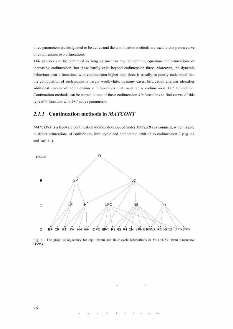
2.1.1 Continuation methods in MATCONT
MATCONT is a freeware continuation toolbox developped under MATLAB environment, which is able
to detect bifurcations of equilibrium, limit cycle and homoclinic orbit up to codimension 2 (Fig. 2.1
and Tab. 2.1).
GPDCPCZH HHBP CP BT GH BPC R3R1 R4 CH LPNS PDNS
PD
EP
O
LP NS
LC
H LPC1
0
codim
2 R2 NSNS LPPD
Figure 1: The graph of adjacency for equilibrium and limit cycle bifurcations in MatCont
NSFNSS NFF ND* TL* SH OF* IF* NCH
HSN
codimLC
HHS
DR*2
1
0
Figure 2: The graph of adjacency for homoclinic bifurcations in MatCont; here * stands forS or U.
general, an arrow from an object of type A to an object of type Bmeans that the object of typeB can be detected (either automatically or by inspecting the output) during the computationof a curve of objects of type A. For example, the arrows from EP to H, LP, and BP meanthat we can detect H, LP and BP during the equilibrium continuation. Moreover, for eacharrow traced in the reversed direction, i.e. from B to A, there is a possibility to start thecomputation of the solution of type A starting from a given object B. For example, startingfrom a BT point, one can initialize the continuation of both LP and H curves. Of course, eachobject of codim 0 and 1 can be continued in one or two system parameters, respectively.
The same interpretation applies to the arrows in Figure 2, where ‘*’ stands for either Sor U, depending on whether a stable or an unstable invariant manifold is involved.
In principle, the graphs presented in Figures 1 and 2 are connected. Indeed, it is knownthat curves of codim 1 homoclinic bifurcations emanate from the BT, ZH, and HH codim 2points. The current version of MatCont fully supports, however, only one such connection:BT ! HHS.
7
Fig. 2.1 The graph of adjacency for equilibrium and limit cycle bifurcations in MATCONT, from Kuznetsov (1995).
27
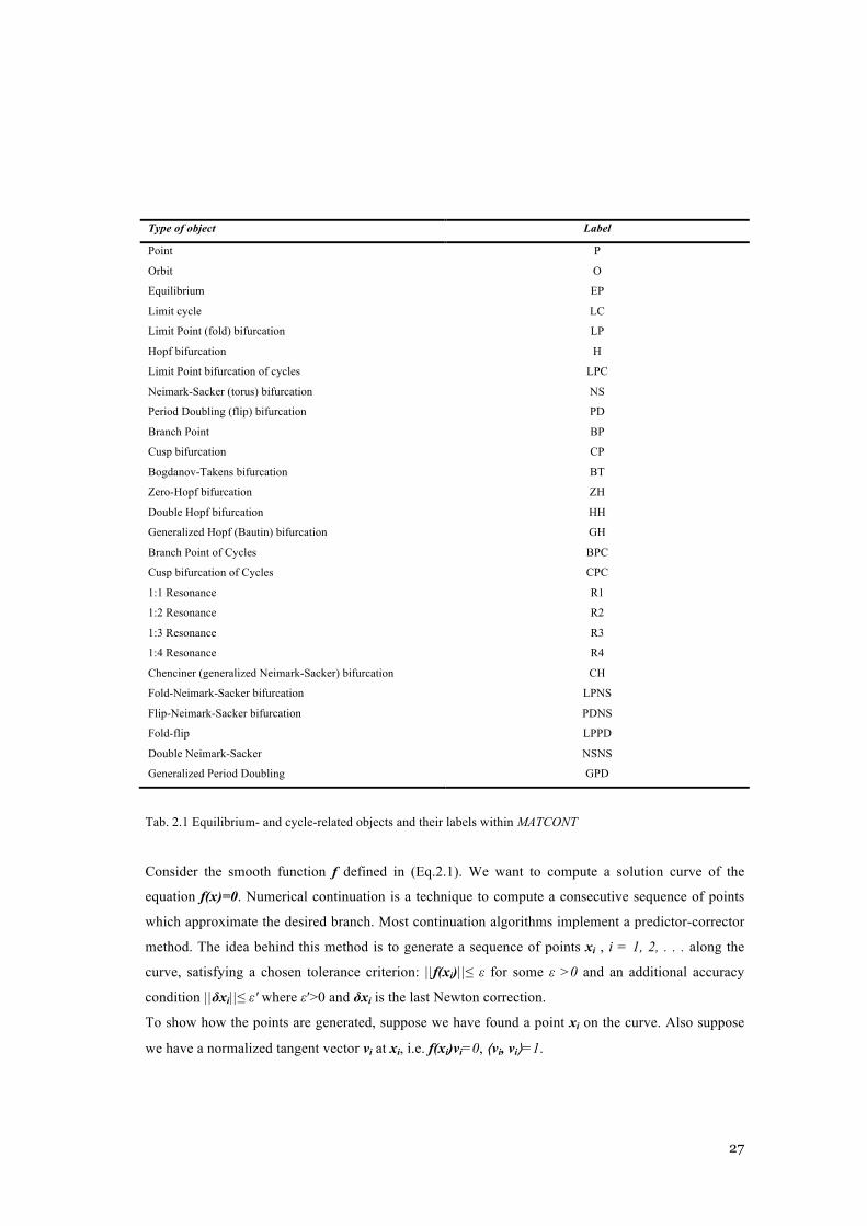
Type of object Label
Point P
Orbit O
Equilibrium EP
Limit cycle LC
Limit Point (fold) bifurcation LP
Hopf bifurcation H
Limit Point bifurcation of cycles LPC
Neimark-Sacker (torus) bifurcation NS
Period Doubling (flip) bifurcation PD
Branch Point BP
Cusp bifurcation CP
Bogdanov-Takens bifurcation BT
Zero-Hopf bifurcation ZH
Double Hopf bifurcation HH
Generalized Hopf (Bautin) bifurcation GH
Branch Point of Cycles BPC
Cusp bifurcation of Cycles CPC
1:1 Resonance R1
1:2 Resonance R2
1:3 Resonance R3
1:4 Resonance R4
Chenciner (generalized Neimark-Sacker) bifurcation CH
Fold-Neimark-Sacker bifurcation LPNS
Flip-Neimark-Sacker bifurcation PDNS
Fold-flip LPPD
Double Neimark-Sacker NSNS
Generalized Period Doubling GPD
Tab. 2.1 Equilibrium- and cycle-related objects and their labels within MATCONT
Consider the smooth function f defined in (Eq.2.1). We want to compute a solution curve of the
equation f(x)=0. Numerical continuation is a technique to compute a consecutive sequence of points
which approximate the desired branch. Most continuation algorithms implement a predictor-corrector
method. The idea behind this method is to generate a sequence of points xi , i = 1, 2, . . . along the
curve, satisfying a chosen tolerance criterion: ||f(xi)||≤ ε for some ε >0 and an additional accuracy
condition ||δxi||≤ ε′ where ε′>0 and δxi is the last Newton correction.
To show how the points are generated, suppose we have found a point xi on the curve. Also suppose
we have a normalized tangent vector vi at xi, i.e. f(xi)vi=0, ⟨vi, vi⟩=1.

28
The computation of the next point xi+1 consists of 2 steps:
• prediction of a new point,
• correction of the predicted point.
The prediction step detects a first guess X0 through the tangent vector vi
X 0 = xi + h ! vi (Eq.2.2)
Assuming that X0 is close to the curve, the point xi+1 on the curve is evaluated through a Newton-like
procedure. Since the standard Newton iterations can only be applied to systems with the same number
of equations as unknowns, an extra scalar condition has to be added:
f (x) = 0g(x) = 0
!"#
$# (Eq.2.3)
The choice of the function g(x) depends on the continuation method adopted. MATCONT uses the
Moore-Penrose method.
Let A be an N×(N+1) matrix with maximal rank. Consider the following linear system with x,v ∈
RN+1,b ∈ RN:
Ax = bvT x = 0
!"#
$# (Eq.2.4)
where x is a point on the curve and v its tangent vector with respect to A, i.e. Av=0. The pseudo-
inverse (or Moore-Penrose inverse) of A, which give the least-square solution for the overdetermined
system Ax=b, is
A+ = AT (AAT )!1 (Eq.2.5)
The solution of (Eq.2.4) is thus x=A+b, because it fulfill the second condition

29
vTA+b = Av, (AAT )!1b = 0 (Eq.2.5)
since v is tangent vector of x with respect to A. Suppose we have a predicted point X0 using (Eq.2.2).
We want to find the point x on the curve which is nearest to X0, i.e. we are trying to solve the
optimization problem minx{||x−X0|| s.t. f(x)=0}.
So, the system we need to solve is:
f (x) = 0wT (x ! X 0 ) = 0
"#$
%$ (Eq.2.6)
where w is the tangent vector at point x. In Newton’s method this system is solved using a
linearization with Taylor expansion about X0:
f (x) = f (X 0 )+ fx (X0 )(x ! X 0 )+o(|| x ! X 0 ||)
wT (x ! X 0 ) = vT (x ! X 0 )+o(|| x ! X 0 ||)
"#$
%$ (Eq.2.7)
So when we discard the higher order terms we can see that the solution of this system is:
x = X 0 ! fx (X0 )+ f (X 0 ) (Eq.2.8)
However, the null vector of fx(X0) is not known, therefore we approximate it by V0=vi, the tangent
vector at xi. Geometrically this means we are solving f(x)=0 in a hyperplane perpendicular to the
previous tangent vector. This is illustrated in Fig. 2.2.
30
V 0
V 1
X0
X2
V 2
X1
xi
xi+1
vi+1
vi
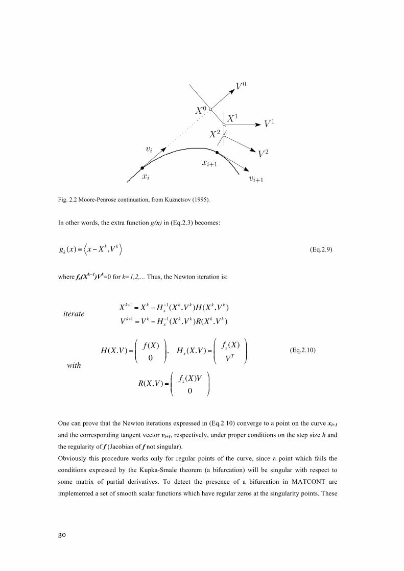
Figure 3: Moore-Penrose continuation
(rank Fx(x) = n). Having found the new point xi+1 on the curve we need to compute thetangent vector at that point:
Fx(xi+1)vi+1 = 0 . (6)
Furthermore the direction along the curve must be preserved: !vi, vi+1" = 1, so we get the(n+ 1)-dimensional appended system
!Fx(xi+1)
vTi
"vi+1 =
!01
". (7)
Upon solving this system, vi+1 must be normalized.
2.2.2 Moore-Penrose continuation
CL MatCont implements a continuation method that is slightly di!erent from the pseudo-arclength continuation.
Definition 1 Let A be an N # (N + 1) matrix with maximal rank. Then the Moore-Penroseinverse of A is defined by A+ = AT (AAT )!1.
Let A be an N # (N + 1) matrix with maximal rank. Consider the following linear systemwith x, v $ RN+1, b $ RN :
Ax = b (8)
vTx = 0 (9)
where x is a point on the curve and v its tangent vector with respect to A, i.e. Av = 0. SinceAA+b = b and vTA+b = !Av, (AAT )!1b" = 0, a solution of this system is
x = A+b. (10)
Suppose we have a predicted point X0 using (1). We want to find the point x on the curvewhich is nearest to X0, i.e. we are trying to solve the optimization problem:
minx
{||x%X0|| | F (x) = 0} (11)
12
Fig. 2.2 Moore-Penrose continuation, from Kuznetsov (1995).
In other words, the extra function g(x) in (Eq.2.3) becomes:
gk (x) = x ! Xk,V k (Eq.2.9)
where fx(Xk−1)Vk=0 for k=1,2,... Thus, the Newton iteration is:
iterateXk+1 = Xk !Hx
!1(Xk,V k )H (Xk,V k )
V k+1 =V k !Hx!1(Xk,V k )R(Xk,V k )
with
H (X,V ) = f (X)0
"
#$$
%
&'', Hx (X,V ) =
fx (X)
VT
"
#$$
%
&''
R(X,V ) = fx (X)V0
"
#$$
%
&''
(Eq.2.10)
One can prove that the Newton iterations expressed in (Eq.2.10) converge to a point on the curve xi+1
and the corresponding tangent vector vi+1, respectively, under proper conditions on the step size h and
the regularity of f (Jacobian of f not singular).
Obviously this procedure works only for regular points of the curve, since a point which fails the
conditions expressed by the Kupka-Smale theorem (a bifurcation) will be singular with respect to
some matrix of partial derivatives. To detect the presence of a bifurcation in MATCONT are
implemented a set of smooth scalar functions which have regular zeros at the singularity points. These
31
functions are called test functions. Suppose we have a singularity S which is detectable by a test
function φ:Rn+1→R. Also assume we have found two consecutive points xi and xi+1 on the curve f(x).
The singularity S will then be detected if φ(xi)φ(xi+1)<0. Having found two points xi and xi+1 one may
want to locate the point x* where φ vanishes. A logical solution is to solve the following system
f (x) = 0!(x) = 0
!"#
$# (Eq.2.11)
using Newton iterations starting at xi. However, to use this method, one should be able to compute the
derivatives of φ(x) which is not always easy. To avoid this difficulty in MATCONT it is implemented
by default a one-dimensional secant method to locate φ(x)=0 along the curve. Notice that this involves
Newton corrections at each intermediate point.
2.2 Simulation methods for non-smooth dynamical sytems
Let formally introduce a definition for piecewise-smooth dynamical systems.
A piecewise-smooth flow is given by a finite set of ODEs
!x = fi (x) for x ! Si (Eq.2.12)
where ∪iSi=D⊂Rn and each Si has a non-empty interior. The intersection ∑ijSi∩Sj is either an Rn-1
dimensional manifold included in the boundaries ∂Sj and ∂Si, or is the empty set. Each vector field fi is
smooth in both the state x and the parameters, and defines a smooth flow Φi(x,t), solution of Eq.2.12,
within any open set U∪Si. In particular, each flow Φi is well defined on both sides of the boundary
∂Si.
A non-empty border between two regions ∑ij will be called a discontinuity set, discontinuity boundary
or, sometimes, a switching manifold. We suppose that each piece of ∑ij is of codimension one, i.e., is
an (n−1) dimensional smooth manifold embedded within the n-dimensional phase space. Moreover,
we shall demand that each such ∑ij is itself piecewise-smooth. That is, it is composed of finitely many
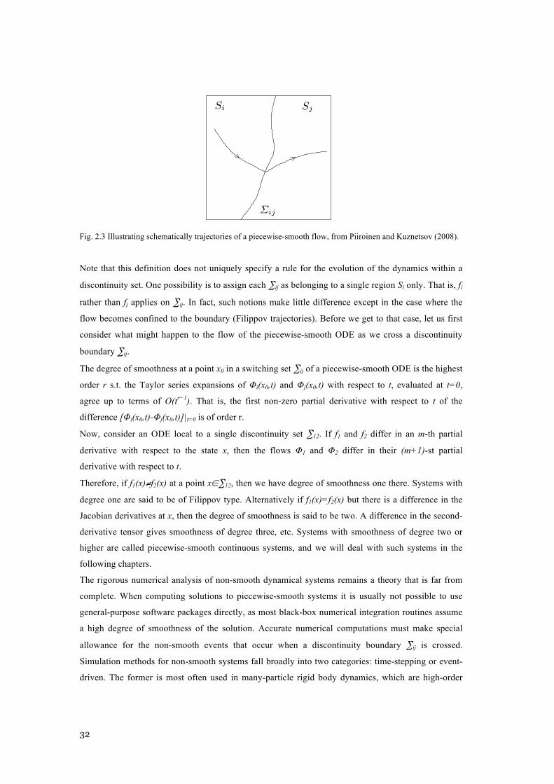
pieces that are as smooth as the flow (see Fig. 2.3).
32
2.2 Piecewise-smooth dynamical systems 73
(a) (b)
S1 S2
!12
Si Sj
!ij
Fig. 2.15. Illustrating schematically trajectories of (a) a piecewise-smooth flow, and(b) a piecewise-smooth map.
2.2.2 Piecewise-smooth ODEs
Definition 2.20. A piecewise-smooth flow is given by a finite set of ODEs
x = Fi(x, µ), for x ! Si, (2.23)
where "iSi = D # Rn and each Si has a non-empty interior. The intersec-tion !ij := Si $ Sj is either an R(n!1)-dimensional manifold included in theboundaries "Sj and "Si, or is the empty set. Each vector field Fi is smoothin both the state x and the parameter µ, and defines a smooth flow #i(x, t)within any open set U % Si. In particular, each flow #i is well defined on bothsides of the boundary "Sj.
A non-empty border between two regions !ij will be called a discontinu-ity set, discontinuity boundary or, sometimes, a switching manifold.We suppose that each piece of !ij is of codimension-one, i.e., is an (n & 1)-dimensional smooth manifold (something locally di!eomorphic to Rn) embed-ded within the n-dimensional phase space. Moreover, we shall demand thateach such !ij is itself piecewise-smooth. That is, it is composed of finitelymany pieces that are as smooth as the flow. See Fig. 2.15(a).
Note that Definition 2.20 does not uniquely specify a rule for the evolutionof the dynamics within a discontinuity set. One possibility is to assign each!ij as belonging to a single region Si only. That is, Fi rather than Fj applieson !ij . In fact, such notions make little di!erence except in the case wherethe flow becomes confined to the boundary (Filippov trajectories). Before weget to that case, let us first consider what might happen to the flow of thepiecewise-smooth ODE as we cross a discontinuity boundary !ij .
Definition 2.21. The degree of smoothness at a point x0 in a switchingset !ij of a piecewise-smooth ODE is the highest order r such the Taylorseries expansions of #i(x0, t) and #j(x0, t) with respect to t, evaluated at t = 0,agree up to terms of O(tr!1). That is, the first non-zero partial derivative withrespect to t of the di!erence [#i(x0, t) & #j(x0, t)]|t=0 is of order r.
Fig. 2.3 Illustrating schematically trajectories of a piecewise-smooth flow, from Piiroinen and Kuznetsov (2008).
Note that this definition does not uniquely specify a rule for the evolution of the dynamics within a
discontinuity set. One possibility is to assign each ∑ij as belonging to a single region Si only. That is, fi
rather than fj applies on ∑ij. In fact, such notions make little difference except in the case where the
flow becomes confined to the boundary (Filippov trajectories). Before we get to that case, let us first
consider what might happen to the flow of the piecewise-smooth ODE as we cross a discontinuity
boundary ∑ij.
The degree of smoothness at a point x0 in a switching set ∑ij of a piecewise-smooth ODE is the highest
order r s.t. the Taylor series expansions of Φi(x0,t) and Φj(x0,t) with respect to t, evaluated at t=0,
agree up to terms of O(tr−1). That is, the first non-zero partial derivative with respect to t of the
difference [Φi(x0,t)-Φj(x0,t)]|t=0 is of order r.
Now, consider an ODE local to a single discontinuity set ∑12. If f1 and f2 differ in an m-th partial
derivative with respect to the state x, then the flows Φ1 and Φ2 differ in their (m+1)-st partial
derivative with respect to t.
Therefore, if f1(x)≠f2(x) at a point x∈∑12, then we have degree of smoothness one there. Systems with
degree one are said to be of Filippov type. Alternatively if f1(x)=f2(x) but there is a difference in the
Jacobian derivatives at x, then the degree of smoothness is said to be two. A difference in the second-
derivative tensor gives smoothness of degree three, etc. Systems with smoothness of degree two or
higher are called piecewise-smooth continuous systems, and we will deal with such systems in the
following chapters.
The rigorous numerical analysis of non-smooth dynamical systems remains a theory that is far from
complete. When computing solutions to piecewise-smooth systems it is usually not possible to use
general-purpose software packages directly, as most black-box numerical integration routines assume
a high degree of smoothness of the solution. Accurate numerical computations must make special
allowance for the non-smooth events that occur when a discontinuity boundary ∑ij is crossed.
Simulation methods for non-smooth systems fall broadly into two categories: time-stepping or event-
driven. The former is most often used in many-particle rigid body dynamics, which are high-order
33
models where there can be perhaps millions of constraints (discontinuities). For such problems, to
accurately solve for events of discontinuity boundary crossing within each time-step and to
subsequently reinitiate the dynamics would be prohibitively computationally expensive. In contrast,
the basic idea of time-stepping is to only check constraints at fixed times at intervals Δt. There are
adaptations to standard methods for integrating ODEs that are specifically designed for such systems.
Clearly, errors are introduced by not accurately detecting the transition times, and therefore time-
stepping schemes are often of low-order accuracy. Several commercially available implementations of
time-stepping algorithms are available, especially for the specific case of rigid body mechanics. These
often have a variational formulation and are able to deal with the difficult problem of the collision of
two rough bodies that may not have unique solutions. See the review by Acary and Brogliato (2008)
for more details.
In the following chapters we will deal with low-dimensional systems with a small number of
discontinuity boundaries. In that context, explicit event-driven schemes are feasible, fast and accurate.
In these methods, trajectories within smooth regions Si are solved using standard numerical integration
algorithms for smooth dynamical systems (e.g., Runge-Kutta, implicit solvers, etc.). Using these
methods, the times at which a discontinuity boundary is hit are accurately solved for, and the problem
is reinitialized there.
A key requirement for an event-driven method is the ability to define each discontinuity boundary as
the zero set of a smooth function Hij(x)=0. Also we have to carefully define a set of transition rules at
each boundary that applies, if necessary, a reset rule Rij and switches to the integration of a new
dynamical system on the far side of the boundary. Thus, the time-integration of a trajectory of the
dynamical system is reduced to the finding of a set of event times tk and events Hij(k) such that
Hij(k)(x(tk))=0.
This can be achieved by setting up a series of monitor functions, the values of which are computed
during each step of the time-integration. If one of these functions changes sign during a time step, then
one needs to use a root finding method to accurately find where Hij=0. These ideas have been
implemented in Matlab by Piiroinen and Kuznetsov (2008).
One of the main uses of direct numerical simulation is to compute the bifurcation diagrams of the set
of attracting solutions directly. In this process, for a fixed parameter value, a set of initial points is
chosen and the flow from each point is determined. The flow is computed for a sufficiently long time
for transients to decay and for the ensuing dynamics to be deemed to have converged onto an attractor.
This dynamics is then recorded, perhaps in a suitable Poincarè section in case of a periodic behaviour
of the system. The parameter is then changed slightly and the same process is repeated. However, an
even more crucial question is to determine what set of initial conditions to take in order to converge to
the various possible attractors. One approach here, which may minimize transient times, is to choose
an initial condition for the new parameter value to be a point on the attractor at the previous parameter
value. However, such an approach will necessarily miss the possibility of competing attractors present

34
in the system. Thus, in general one should start from a range of different points within a suitably
defined subset D of the phase space from which one has a priori knowledge that the attractors of the
system must lie. The number of points should of course be chosen to be as large as possible for the
computational time available. One could start with a regular grid of points, but there are advantages in
choosing the initial points at random. That is, at each fixed parameter value, use a random number
generator to choose initial conditions in D uniformly. This way, the situation where attractors with
small basins of attraction are missed consistently at each parameter value are likely to be avoided. We
will refer to this method for computing bifurcation diagrams as a Monte Carlo method. The direct
simulation method has many advantages in giving a quick and realistic picture of the bifurcation
diagram of a system without assuming any a priori structure about the number or form of the
attractors.
35
3 MODELS DESCRIPTION AND
ANALYSIS
In this chapter will be described in details the two eco-hydrological models that has been developed.
The first model (TGSN) deals with the role of competition between different plant functional types
(namely woody and herbaceous plant) for the two most limiting resources in tropical and subtropical
biomes (soil moisture and mineral nitrogen). The second model (SNPV) neglect the role of
competition in order to address the interaction between the hydrological cycle and the biogeochemical
cycle of nitrogen and phosphorous, and the condition for the limitation of nutrient to vegetation
growth. The equations of both models are described in details, and their qualitative behaviour is
analyzed using the numerical tools described in the previous chapter.
36
3.1 TGSN model: introduction and bifurcation analysis
A dynamical model of tree-grass-soil water-mineral nitrogen interactions, in a given volume of soil, is
introduced here. It describes locally the temporal dynamics of tree and grass in presence of two
resources: soil water and mineral nitrogen.
Let z indicate the root zone depth, n the porosity (fractional pore volume), w the control volume
having unit area and depth z, w = 1 × z, wp the pore space in the volume w, wp = 1 × z × n=1 × w1,
with w1= z × n.
The water table is assumed to be deep enough to not affect the water dynamics in the root zone. The
dynamics of soil water is described through the mass balance equation of the water present in the
control volume relative to the maximum water that can be held in this volume. This dimensionless
quantity S (‘degree of saturation’) ranges in the interval [0, 1]. S=0 corresponds to completely dry
soil, and S=1 to completely saturated soil. The soil water balance equation is
( ) SGSTSSwP
dtdS
GT τ−τ−ε−−= 11
(Eq.3.1)
In Eq.3.1, the term P/w1 represents the rainfall rate normalized with respect to the root zone capacity.
Here, P (P≥0, mm/yr) is assumed constant in the year (i.e, P is the mean annual rainfall). Following
De Michele et al. (2008), we assume that the soil surface is more-or-less horizontal, and the whole
amount of rainfall infiltrates the soil as long as the soil water holding capacity is not exceeded. The
term P/w1S models the deep percolation, beyond the rooting zone. When S=0 (completely dry soil) all
the rainfall contributes to moistening of the root zone. When S=1 (saturated root zone) the rainfall
runs off or percolates through the soil towards the water table, and it is no longer available to the
vegetation at this location. The term εS models the evaporation from the soil. The term τTST (τGSG)
models water uptake by the vegetation as proportional to S and the vegetation quantity T (G).
The dynamics of the nitrogen are described through the mass balance equation of mineral nitrogen in
the soil per unit area, indicated by N (N≥0, gN/m2):
NGcNTcaNQdtdN
GT −−−= (Eq.3.2)
37
In Eq.3.2, Q (gN/m2/yr) is the rate of nitrogen supply. This is principally by mineralization of organic
nitrogen in the soil, but also has a component of wet and dry deposition of atmospherically-borne
nitrogen and biological nitrogen fixation. In the long term, there is a feedback between the vegetation
quantity (T and G) and the amount of soil organic nitrogen that provided the substrate for Q, but the
stock of soil organic nitrogen is much bigger than either T or G or the flux Q, so for simplicity this
mechanism is subsumed in the net uptake term. aN is a loss term due to leaching and gaseous losses
such as volatilization and denitrification. The nitrogen uptake of plants is represented by two terms
proportional to the nutrient mass, and the plant abundance, cTNT and cGNT, respectively for tree and
grass. The consumption of the two resources is a complex combination of simultaneous and
independent uptake, since the soil water is both a necessary growth resource and a vehicle for nutrient
uptake through water-mediated bulk flow, while the active transport to the xylem and mychorrhizal-
mediated transport are independent component of the consumption vector (Gleeson and Tilman 1992).
In order to represent this behavior in a simple way, the consumption rates for the inorganic nitrogen
are assumed independent of the transpiration rates, but the consumption vectors of both plant forms
are not assumed to follow the optimal foraging condition, i.e. that essential resources should be
consumed in the proportion for which the population would be equally limited by both resources
(Tilman 1982).
The dynamics of vegetation T (G) is described through a mass balance between the growth and the
death of vegetation. Here, the growth rate of T (G) is proportional to the consumed water, w1τTST
(w1τGSG), multiplied by a conversion coefficient ηT (ηG) that depends on the nitrogen content per unit
of water uptake (that is, the nitrogen concentration), cTNT ! Tw1ST ( cGNG !Gw1SG ). According to
Larcher (2003), since the plant response to a mineral nutrient depends by its concentration and not by
its absolute quantity, we assume that the conversion coefficient ηT (ηG) is zero for scarce values of
nitrogen concentration, while it saturates to a maximum when the nitrogen concentration increases
according to the Holling II type function,
!i =!imax "i ciN # iw1S1+"i ciN # iw1S
with i = T,G (Eq.3.3)
where αT (αG) is a parameter representing the velocity of saturation. We neglect the effect of
excessive concentration, leading to depressive effects on growth, since we assume environments
characterized by nitrogen scarcity.
The death rate of tree (grass) is proportional to T (G) with a coefficient µT (µG). In addition, we have a
direct effect of tree on the grassy layer, modeled by an additional death rate proportional to TG with a
coefficient δ. Thus, the tree dynamics can be expressed as follows:

38
( )max 1
1
,T T TT T T
T T T
w c SNdT T T S N Tdt w S c N
τ αη µ φ
τ α= − =
+ (Eq.3.4)
while the grass dynamics is
( )max 1
1
, ,G G GG G G
G G G
w c SNdG G G TG S N T Gdt w S c N
τ αη µ δ φ
τ α= − − =
+ (Eq.3.5)
The growth functions of tree and grass can be described in term of their isoclines on the S-N plane,
particularly the zero growth isoclines (ZGI) that play a crucial role on the stability of the system’s
steady states. The ZGI present horizontal and vertical asymptotes for the values
ST* =
µT !Tmax
! Tw1
NT* =
µT !Tmax
!TcT
!
"
##
$
##
andSG* =
µG %!T( ) !Gmax
!Gw1
NG* =
µG %!T( ) !Gmax
!GcG
!
"
##
$
##
(Eq.3.6)
Fig. 3.1 shows an indicative shape for the ZGI of the two functional types, and taking T=0 for the
representation of the ZGI relative to the grass. So according to Hypothesis 1, in conditions of low
nitrogen but high water availability, φT has zero growth isocline nearer to the origin than φG, and the
converse is true for high nitrogen, low water conditions. Obviously, the ZGIs under Hypothesis 2 are
switched: in conditions of low nitrogen but high water availability, φG has zero growth isocline nearer
to the origin than φT, and the converse is true for high nitrogen, low water conditions.
39
Fig. 3.1 Resource-dependent isoclines for the two functional type. In Hypothesis 1, φ1=φT and φ2=φG, while in Hypothesis 2 φ1=φG and φ2=φT .
The interactions among tree-grass-water-nitrogen variables are represented by a fourth order system of
non-linear ordinary differential equations:
( )
max
max
1
1
1
1
1
1 T G
T G
T T TT T
T T T
G G GG G
G G G
dS P S S ST SGdt wdN Q aN c NT c NGdt
w c SNdT Tdt w S c N
w c SNdG T Gdt w S c N
ε τ τ
τ αη µ
τ α
τ αη µ δ
τ α
⎧ = − − − −⎪⎪⎪
= − − −⎪⎪⎨ ⎛ ⎞⎪ = −⎜ ⎟
+⎪ ⎝ ⎠⎪
⎛ ⎞⎪ = − −⎜ ⎟⎪ +⎝ ⎠⎩
(Eq.3.7)
Fig. 3.2 shows the nature of the dependencies among the state variables, T, G, S, N.
40
Fig. 3.2 Graph of influences for the state variables.
The steady states are indicated with the symbol “E”, and two superscripts q1q2 : the first referring to the
tree state, and the second to the grass state. Each steady state, Eq1q2 , is a 1×4 matrix
Eq1q2 ! (Sq1q2 ,Nq1q2 ,T q1q2 ,Gq1q2 ) . Each superscript can be 0 or 1. When a superscript is equal to 0, the
correspondent vegetation is extinct (i.e., q1=0 ↔ T=0, or q2=0 ↔ G=0), when a superscript is equal to
1, the correspondent vegetation is resources controlled, i.e., one or both of the resources limit the
vegetation to a steady state with positive biomass (q1=1 ↔ T>0, or q2=1 ↔ G>0). Thus, the tree-grass
dynamics is conditioned by: 1) the limiting effect of the resources availability, and 2) the limiting
effect of the abundance of the conspecific (Keymer et al. 2008). The system described by Eq.3.7 has
four steady states. One of these has both q1 and q2 equal to 0, representing bare soil, which is a trivial
solution for our purposes. The other three solutions, namely E 01,E10,E11 , represent non trivial
vegetation outcomes: resource-limited but treeless grassland, a grassless but resource-limited forest or
thicket, and a savanna in which both trees and grass are resource-constrained. The complete set of
steady states is summarized in Tab. 3.1.
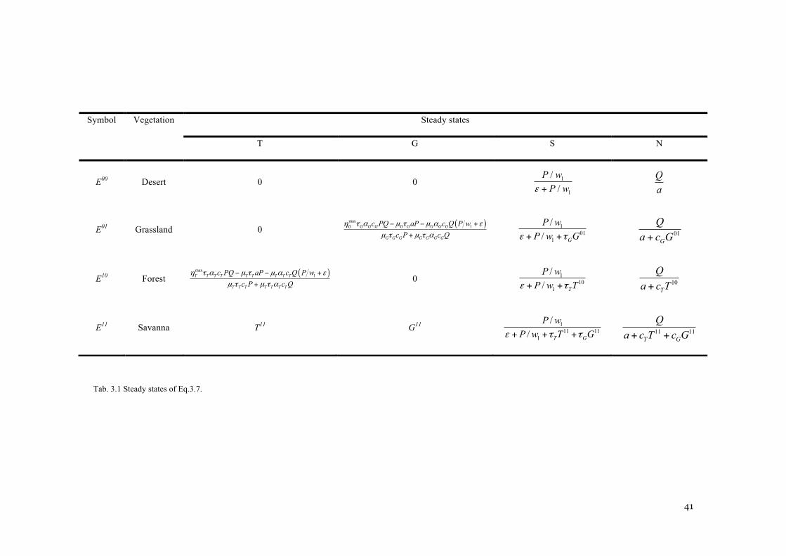
41
Tab. 3.1 Steady states of Eq.3.7.
Symbol Vegetation Steady states
T G S N
E00 Desert 0 0 1
1
//
P wP wε +
Qa
E01 Grassland 0 ( )max1G G G G G G G G G
G G G G G G G
c PQ aP c Q P wc P c Q
η τ α µ τ µ α εµ τ µ τ α− − +
+ 1
011
// G
P wP w G+ +ε τ 01
G
Qa c G+
E10 Forest ( )max1T T T T T T T T T
T T T T T T T
c PQ aP c Q P wc P c Q
η τ α µ τ µ α εµ τ µ τ α− − +
+ 0 1
101
// T
P wP w T+ +ε τ 10
T
Qa c T+
E11 Savanna T11 G11 111 11
1
// T G
P wP w T G+ + +ε τ τ 11 11
T G
Qa c T c G+ +
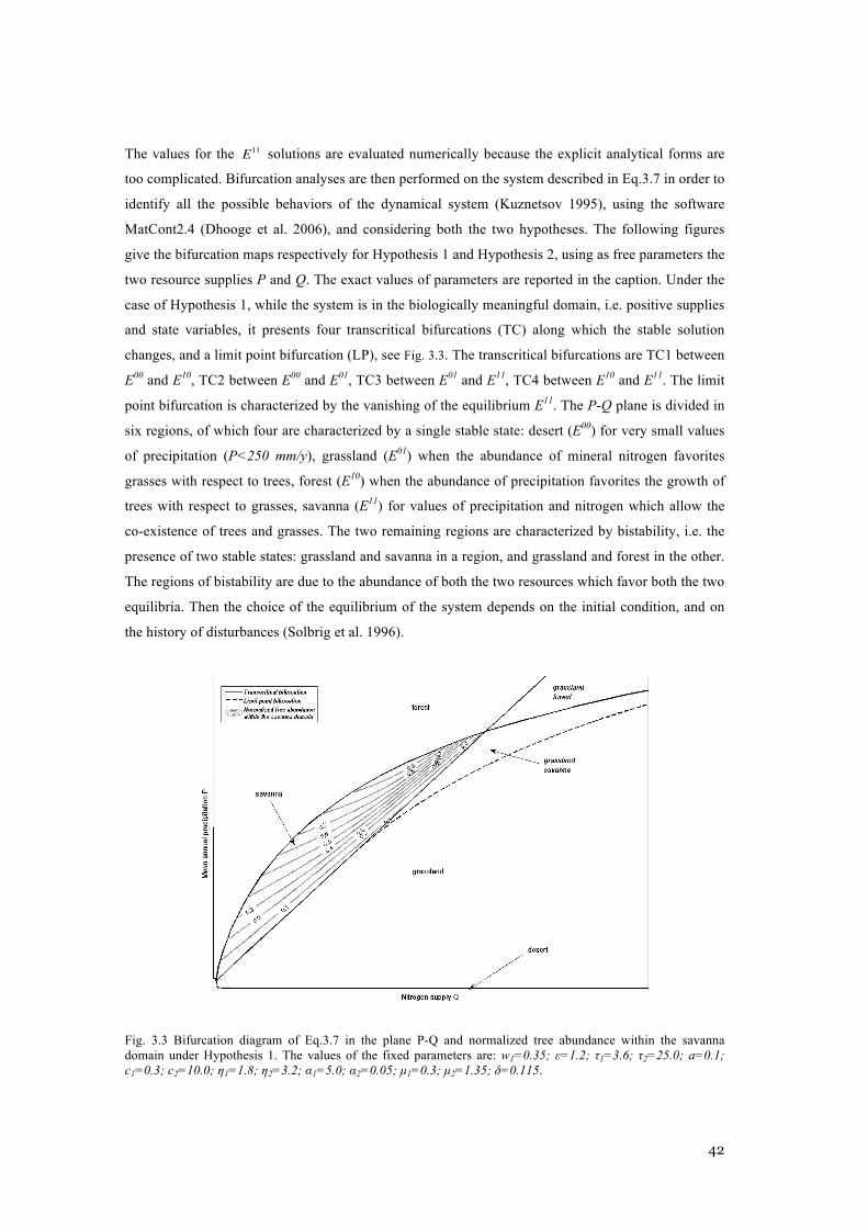
42
The values for the E11 solutions are evaluated numerically because the explicit analytical forms are
too complicated. Bifurcation analyses are then performed on the system described in Eq.3.7 in order to
identify all the possible behaviors of the dynamical system (Kuznetsov 1995), using the software
MatCont2.4 (Dhooge et al. 2006), and considering both the two hypotheses. The following figures
give the bifurcation maps respectively for Hypothesis 1 and Hypothesis 2, using as free parameters the
two resource supplies P and Q. The exact values of parameters are reported in the caption. Under the
case of Hypothesis 1, while the system is in the biologically meaningful domain, i.e. positive supplies
and state variables, it presents four transcritical bifurcations (TC) along which the stable solution
changes, and a limit point bifurcation (LP), see Fig. 3.3. The transcritical bifurcations are TC1 between
E00 and E10, TC2 between E00 and E01, TC3 between E01 and E11, TC4 between E10 and E11. The limit
point bifurcation is characterized by the vanishing of the equilibrium E11. The P-Q plane is divided in
six regions, of which four are characterized by a single stable state: desert (E00) for very small values
of precipitation (P<250 mm/y), grassland (E01) when the abundance of mineral nitrogen favorites
grasses with respect to trees, forest (E10) when the abundance of precipitation favorites the growth of
trees with respect to grasses, savanna (E11) for values of precipitation and nitrogen which allow the
co-existence of trees and grasses. The two remaining regions are characterized by bistability, i.e. the
presence of two stable states: grassland and savanna in a region, and grassland and forest in the other.
The regions of bistability are due to the abundance of both the two resources which favor both the two
equilibria. Then the choice of the equilibrium of the system depends on the initial condition, and on
the history of disturbances (Solbrig et al. 1996).
Fig. 3.3 Bifurcation diagram of Eq.3.7 in the plane P-Q and normalized tree abundance within the savanna domain under Hypothesis 1. The values of the fixed parameters are: w1=0.35; ε=1.2; τ1=3.6; τ2=25.0; a=0.1; c1=0.3; c2=10.0; η1=1.8; η2=3.2; α1=5.0; α2=0.05; µ1=0.3; µ2=1.35; δ=0.115.
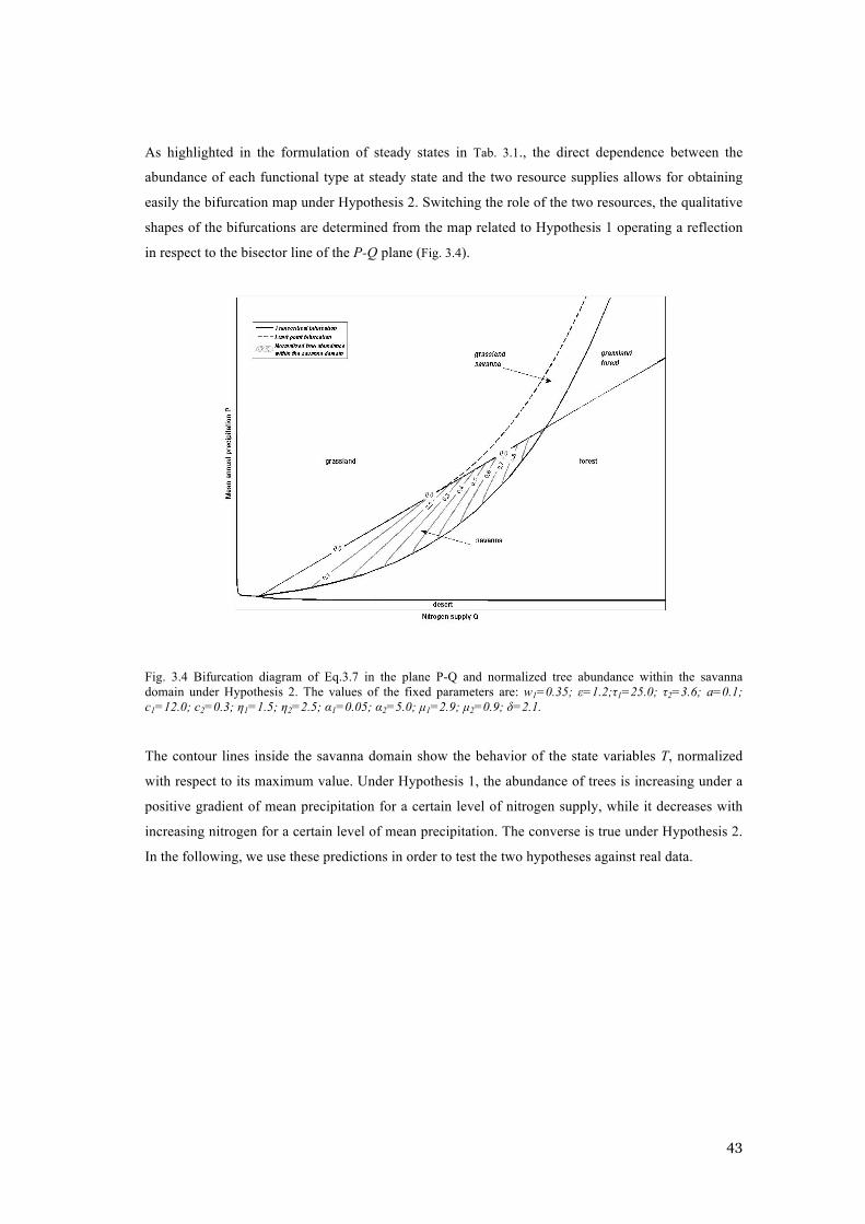
43
As highlighted in the formulation of steady states in Tab. 3.1., the direct dependence between the
abundance of each functional type at steady state and the two resource supplies allows for obtaining
easily the bifurcation map under Hypothesis 2. Switching the role of the two resources, the qualitative
shapes of the bifurcations are determined from the map related to Hypothesis 1 operating a reflection
in respect to the bisector line of the P-Q plane (Fig. 3.4).
Fig. 3.4 Bifurcation diagram of Eq.3.7 in the plane P-Q and normalized tree abundance within the savanna domain under Hypothesis 2. The values of the fixed parameters are: w1=0.35; ε=1.2;τ1=25.0; τ2=3.6; a=0.1; c1=12.0; c2=0.3; η1=1.5; η2=2.5; α1=0.05; α2=5.0; µ1=2.9; µ2=0.9; δ=2.1.
The contour lines inside the savanna domain show the behavior of the state variables T, normalized
with respect to its maximum value. Under Hypothesis 1, the abundance of trees is increasing under a
positive gradient of mean precipitation for a certain level of nitrogen supply, while it decreases with
increasing nitrogen for a certain level of mean precipitation. The converse is true under Hypothesis 2.
In the following, we use these predictions in order to test the two hypotheses against real data.
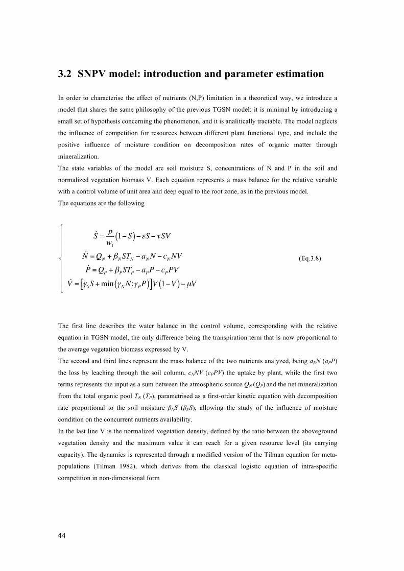
44
3.2 SNPV model: introduction and parameter estimation
In order to characterise the effect of nutrients (N,P) limitation in a theoretical way, we introduce a
model that shares the same philosophy of the previous TGSN model: it is minimal by introducing a
small set of hypothesis concerning the phenomenon, and it is analitically tractable. The model neglects
the influence of competition for resources between different plant functional type, and include the
positive influence of moisture condition on decomposition rates of organic matter through
mineralization.
The state variables of the model are soil moisture S, concentrations of N and P in the soil and
normalized vegetation biomass V. Each equation represents a mass balance for the relative variable
with a control volume of unit area and deep equal to the root zone, as in the previous model.
The equations are the following
!S = pw11! S( )!!S !!SV
!N =QN +!NSTN ! aNN ! cNNV!P =QP +!PSTP ! aPP ! cPPV
!V = !SS +min !NN;!PP( )"# $%V 1!V( )!µV
&
'
(((
)
(((
(Eq.3.8)
The first line describes the water balance in the control volume, corresponding with the relative
equation in TGSN model, the only difference being the transpiration term that is now proportional to
the average vegetation biomass expressed by V.
The second and third lines represent the mass balance of the two nutrients analyzed, being aNN (aPP)
the loss by leaching through the soil column, cNNV (cPPV) the uptake by plant, while the first two
terms represents the input as a sum between the atmospheric source QN (QP) and the net mineralization
from the total organic pool TN (TP), parametrised as a first-order kinetic equation with decomposition
rate proportional to the soil moisture βNS (βPS), allowing the study of the influence of moisture
condition on the concurrent nutrients availability.
In the last line V is the normalized vegetation density, defined by the ratio between the aboveground
vegetation density and the maximum value it can reach for a given resource level (its carrying
capacity). The dynamics is represented through a modified version of the Tilman equation for meta-
populations (Tilman 1982), which derives from the classical logistic equation of intra-specific
competition in non-dimensional form
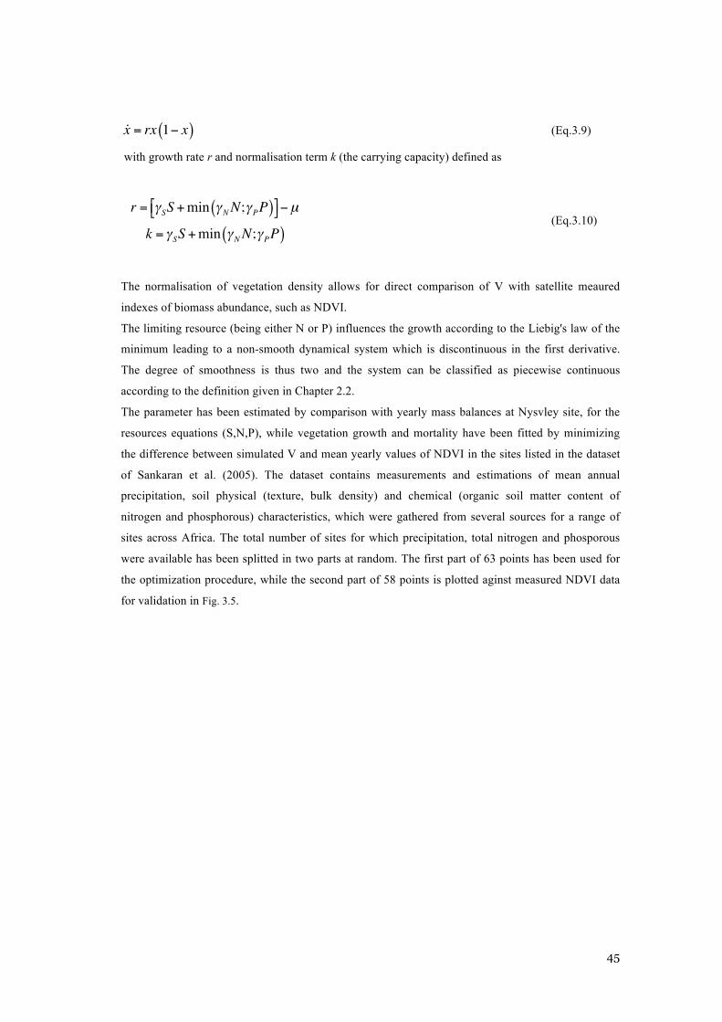
45
!x = rx 1! x( ) (Eq.3.9)
with growth rate r and normalisation term k (the carrying capacity) defined as
r = !SS +min !NN;!PP( )!" #$%µ
k = !SS +min !NN;!PP( ) (Eq.3.10)
The normalisation of vegetation density allows for direct comparison of V with satellite meaured
indexes of biomass abundance, such as NDVI.
The limiting resource (being either N or P) influences the growth according to the Liebig's law of the
minimum leading to a non-smooth dynamical system which is discontinuous in the first derivative.
The degree of smoothness is thus two and the system can be classified as piecewise continuous
according to the definition given in Chapter 2.2.
The parameter has been estimated by comparison with yearly mass balances at Nysvley site, for the
resources equations (S,N,P), while vegetation growth and mortality have been fitted by minimizing
the difference between simulated V and mean yearly values of NDVI in the sites listed in the dataset
of Sankaran et al. (2005). The dataset contains measurements and estimations of mean annual
precipitation, soil physical (texture, bulk density) and chemical (organic soil matter content of
nitrogen and phosphorous) characteristics, which were gathered from several sources for a range of
sites across Africa. The total number of sites for which precipitation, total nitrogen and phosporous
were available has been splitted in two parts at random. The first part of 63 points has been used for
the optimization procedure, while the second part of 58 points is plotted aginst measured NDVI data
for validation in Fig. 3.5.
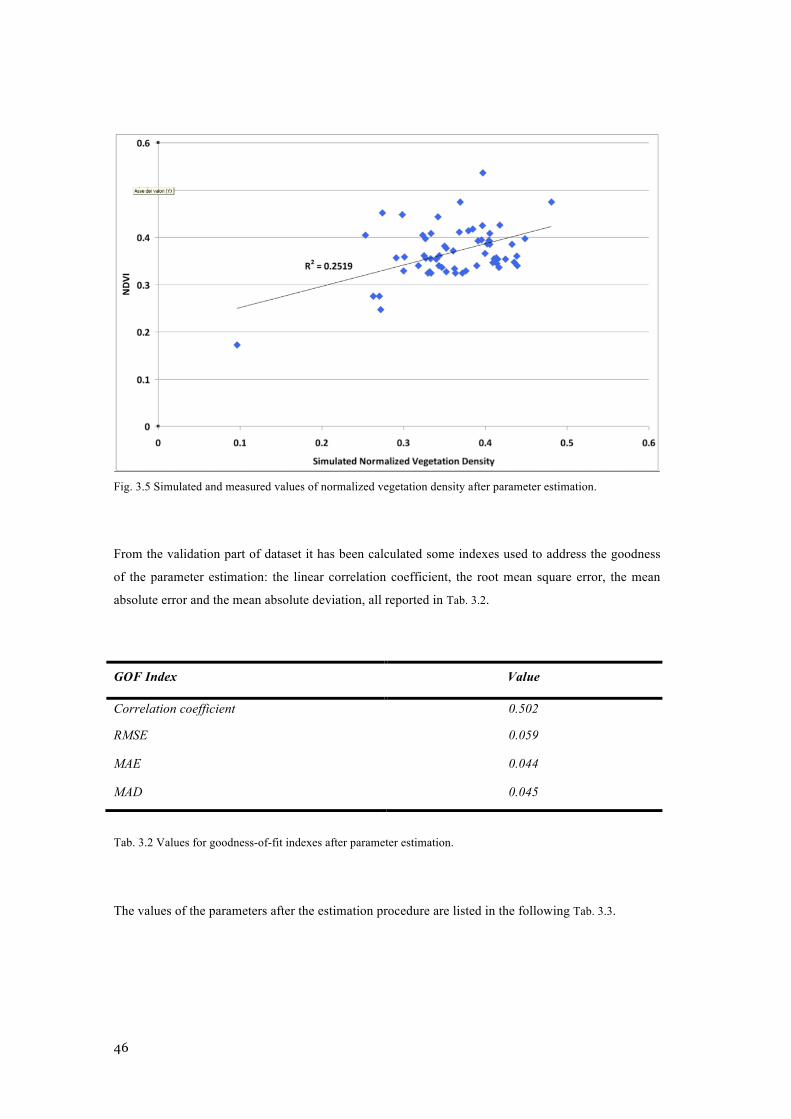
46
Fig. 3.5 Simulated and measured values of normalized vegetation density after parameter estimation.
From the validation part of dataset it has been calculated some indexes used to address the goodness
of the parameter estimation: the linear correlation coefficient, the root mean square error, the mean
absolute error and the mean absolute deviation, all reported in Tab. 3.2.
GOF Index Value
Correlation coefficient 0.502
RMSE 0.059
MAE 0.044
MAD 0.045
Tab. 3.2 Values for goodness-of-fit indexes after parameter estimation.
The values of the parameters after the estimation procedure are listed in the following Tab. 3.3.
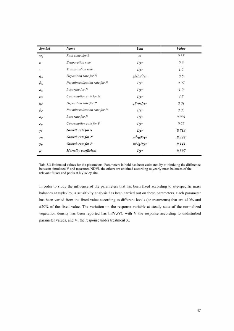
47
Symbol Name Unit Value
w1 Root zone depth m 0.35
ε Evaporation rate 1/yr 0.6
τ Transpiration rate 1/yr 1.5
qN Deposition rate for N gN/m2/yr 0.8
βN Net mineralization rate for N 1/yr 0.07
aN Loss rate for N 1/yr 1.0
cN Consumption rate for N 1/yr 4.7
qP Deposition rate for P gP/m2/yr 0.01
βP Net mineralization rate for P 1/yr 0.03
aP Loss rate for P 1/yr 0.001
cP Consumption rate for P 1/yr 0.25
γS Growth rate for S 1/yr 0.713
γN Growth rate for N m2/gN/yr 0.324
γP Growth rate for P m2/gP/yr 0.141
µ Mortality coefficient 1/yr 0.307
Tab. 3.3 Estimated values for the parameters. Parameters in bold has been estimated by minimizing the difference between simulated V and measured NDVI, the others are obtained according to yearly mass balances of the relevant fluxes and pools at Nylsvley site.
In order to study the influence of the parameters that has been fixed according to site-specific mass
balances at Nylsvley, a sensitivity analysis has been carried out on these parameters. Each parameter
has been varied from the fixed value according to different levels (or treatments) that are ±10% and
±20% of the fixed value. The variation on the response variable at steady state of the normalized
vegetation density has been reported has ln(Vx/V), with V the response according to undisturbed
parameter values, and Vx the response under treatment X.
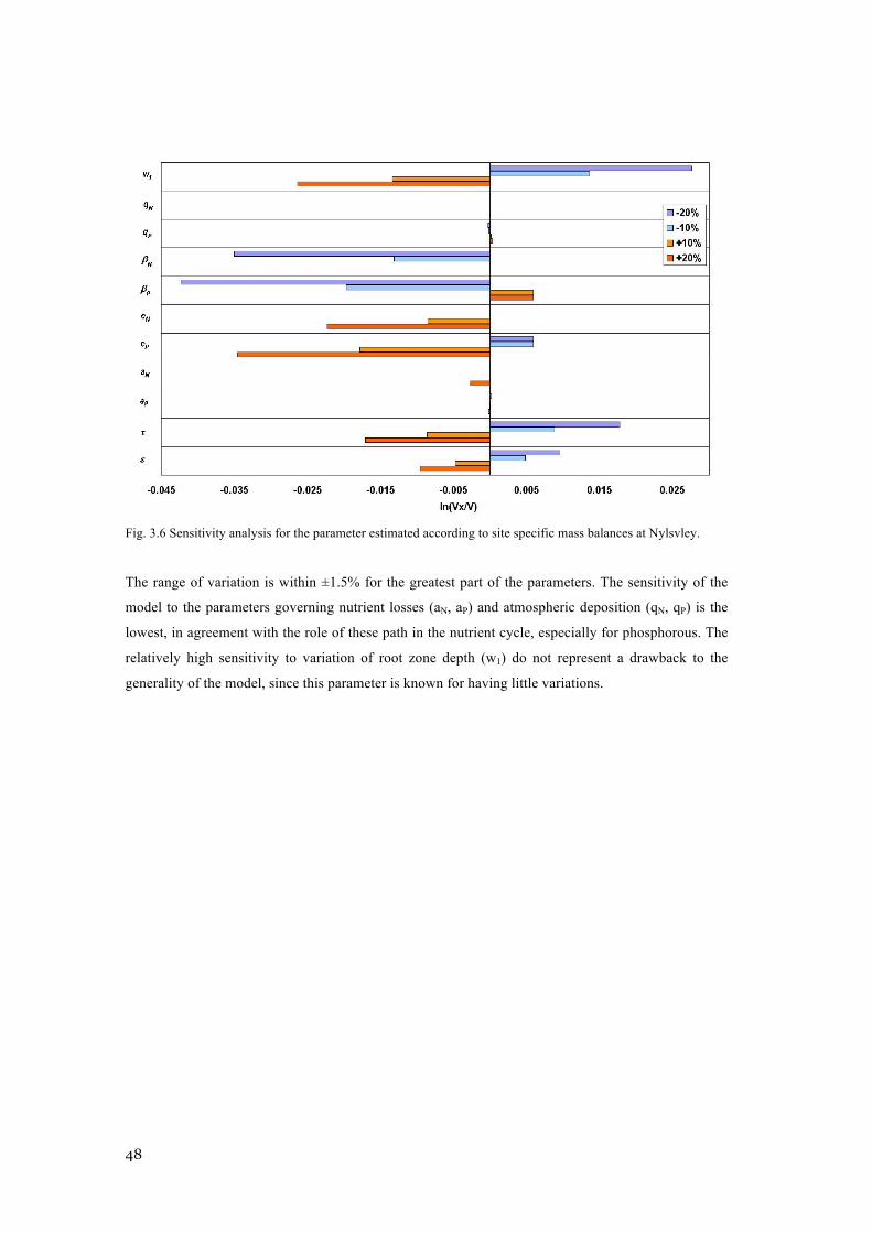
48
Fig. 3.6 Sensitivity analysis for the parameter estimated according to site specific mass balances at Nylsvley.
The range of variation is within ±1.5% for the greatest part of the parameters. The sensitivity of the
model to the parameters governing nutrient losses (aN, aP) and atmospheric deposition (qN, qP) is the
lowest, in agreement with the role of these path in the nutrient cycle, especially for phosphorous. The
relatively high sensitivity to variation of root zone depth (w1) do not represent a drawback to the
generality of the model, since this parameter is known for having little variations.
49
4 DATA COMPARISON AND RESULTS
In this chapter the two models are used in order to address specific eco-hydrogical problems. In
particular, the problem of the definition of competition status of trees and grasses with respect to soil
moisture and nitrogen is addressed in a formal way by using the results from the TGSN model.
Furthermore, the model is compared with a global dataset, showing that it can lead to a simple
understanding of global patterns of biome distribution in the world.
Finally, the behaviour of the SNPV is analyzed with respect to nutrient enrichment experiments,
which represent the main source of observation on the topic of nutrient limitation.
50
4.1 TGSN model: testing competition status hypotheses
In order to understand if Hypothesis 1 (H1) or Hypothesis 2 (H2) can represent, or not, observed data,
we test these two contrasting hypotheses against the dataset described in Sankaran et al. (2005). The
dataset contains measurements and estimations of projected woody cover (the percentage of ground
surface covered when crowns are projected vertically), MAP, soil characteristics (texture, total
nitrogen and phosphorus, and nitrogen mineralization), fire and herbivory regimes, which were
gathered from several sources for a range of sites across Africa.
Here we focus the attention on three variables: woody cover, mean annual precipitation and potential
N mineralization. This because the woody cover is a proxy of tree abundance; the mean annual
precipitation is an indicator of water supply, and the potential N mineralization, quantified following
laboratory incubations of soils under anaerobic conditions, is an index of N availability and turnover
in soils, a good predictor of the annual N mineralization (Schaffers, 2000). Unfortunately we have not
measurements of the model’s variables, however we can work with measured values of proxy
variables. Here we assume unknown increasing functions between the proxy variables (i.e. woody
cover and potential N mineralization) and the model variables (i.e. tree abundance in term of
aboveground biomass and annual N mineralization).
In addition we group data, according to the soil type, in sandy, loamy and clayly soil, as estimated
through the content of sand and clay. For each soil type, some sections in the P-Q plane are considered
in correspondence of fixed values of one resource (precipitation or nitrogen) and selecting all the data
points within an interval of size Δ centered in the fixed value. For each vertical (constant nitrogen) and
horizontal (constant precipitation) section we estimate the dependence between the woody cover and
the other (non-constant) resource. In particular we use the Kendall’s τ, which is a non-parametric
rank-based measure of association, invariant under monotonic transformations of data (Salvadori et al.
2007), of interest here, because we are working with proxy data. Under the condition of null
association (H0), the sampling distribution of Kendall’s τ is approximately normal distributed with 0
mean and variance equal to
!"2 =
2(2N + 5)9N(N !1)
(Eq.4.1)
where N is the sample size. Using this information it is possible to test the independence, or null
association, between two variables: if the estimate of τ is out the confidence interval (having the above
indicated mean and variance and a level of significance generally assumed equal to 1% and 5%) then

51
the association is to be considered statistically significant (Press et al. 1992). This test is known as
Kendall’s test of independence, and considered in the following.
The model, under Hypothesis 1, is characterized by increasing values of woody cover increasing the
values of precipitation along vertical sections (i.e. positive values of τ) and by decreasing values of
woody cover increasing the values of nitrogen along horizontal sections, (i.e. negative values of τ).
Conversely the model under Hypothesis 2 is characterized by τ<0 along vertical sections, and τ>0
along horizontal sections.
To investigate the model’s behavior, using alternatively Hypothesis 1 (H1) and Hypothesis 2 (H2),
against data, we apply the Kendall’s test of independence to the sample values of Kendall’s τ, between
woody cover and resource level (precipitation and nitrogen), for 13 sections identified and reported in
Tab. 4.1. In particular,
• for sections at a fixed value of nitrogen, if the sample Kendall’s τ is significantly >0 we can
reject H0 in favor of H1; conversely if τ is significantly <0 then we can reject H0 in favor of H2;
• for sections at a fixed value of precipitation, if the Kendall’s τ is significantly <0 we can reject
H0 in favor of H1; conversely if τ is significantly >0 then we can reject H0 in favor of H2;
Fig. 4.1 shows the test through box-and-whiskers plots, providing the inter-quartile range (the box) and
the 99-percentile range (the whiskers) and the sample estimates of Kendall’s τ (the dots) for all the
sections considered.
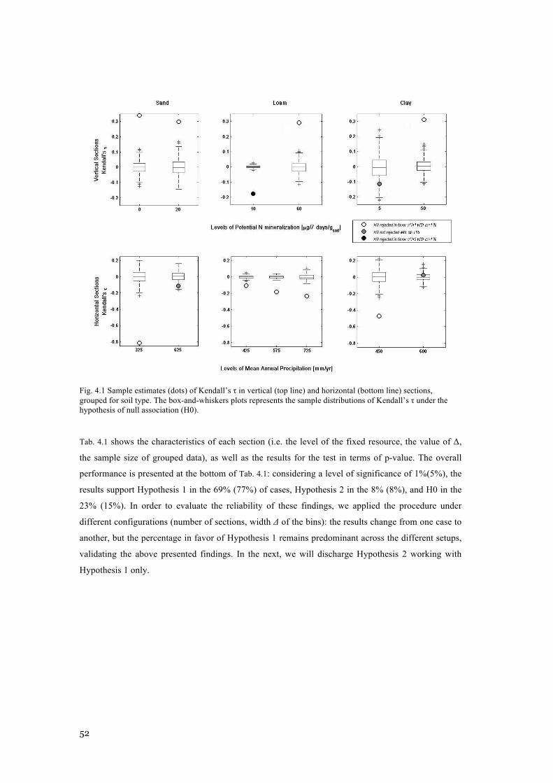
52
Fig. 4.1 Sample estimates (dots) of Kendall’s τ in vertical (top line) and horizontal (bottom line) sections, grouped for soil type. The box-and-whiskers plots represents the sample distributions of Kendall’s τ under the hypothesis of null association (H0).
Tab. 4.1 shows the characteristics of each section (i.e. the level of the fixed resource, the value of Δ,
the sample size of grouped data), as well as the results for the test in terms of p-value. The overall
performance is presented at the bottom of Tab. 4.1: considering a level of significance of 1%(5%), the
results support Hypothesis 1 in the 69% (77%) of cases, Hypothesis 2 in the 8% (8%), and H0 in the
23% (15%). In order to evaluate the reliability of these findings, we applied the procedure under
different configurations (number of sections, width Δ of the bins): the results change from one case to
another, but the percentage in favor of Hypothesis 1 remains predominant across the different setups,
validating the above presented findings. In the next, we will discharge Hypothesis 2 working with
Hypothesis 1 only.
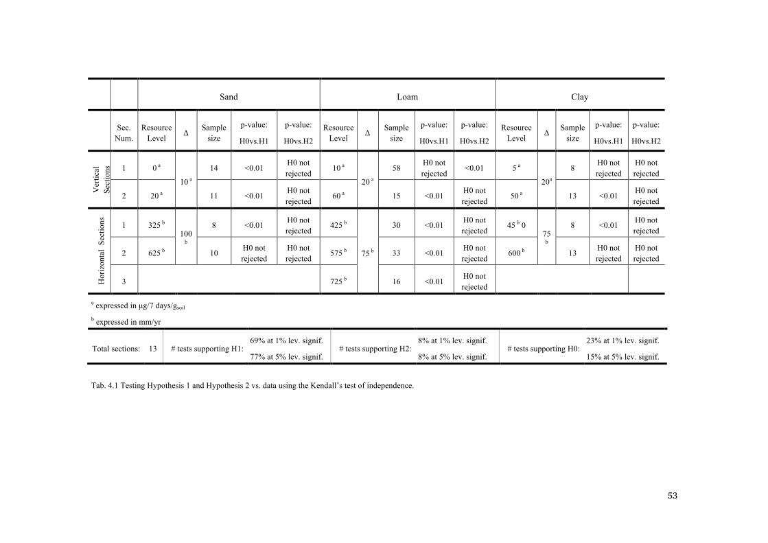
53
Sand Loam Clay
Sec. Num.
Resource Level
Δ Sample size
p-value:
H0vs.H1
p-value:
H0vs.H2
Resource Level
Δ Sample size
p-value:
H0vs.H1
p-value:
H0vs.H2
Resource Level
Δ Sample size
p-value:
H0vs.H1
p-value:
H0vs.H2
Ver
tical
Se
ctio
ns 1 0 a
10 a
14 <0.01 H0 not rejected
10 a
20 a
58 H0 not rejected
<0.01 5 a
20a
8 H0 not rejected
H0 not rejected
2 20 a 11 <0.01 H0 not rejected
60 a 15 <0.01 H0 not rejected
50 a 13 <0.01 H0 not rejected
Hor
izon
tal
Sect
ions
1 325 b 100
b
8 <0.01 H0 not rejected
425 b
75 b
30 <0.01 H0 not rejected
45 b 0 75
b
8 <0.01 H0 not rejected
2 625 b 10 H0 not rejected
H0 not rejected
575 b 33 <0.01 H0 not rejected
600 b 13 H0 not rejected
H0 not rejected
3 725 b 16 <0.01 H0 not rejected
a expressed in µg/7 days/gsoil
b expressed in mm/yr
Total sections: 13 # tests supporting H1: 69% at 1% lev. signif.
77% at 5% lev. signif. # tests supporting H2:
8% at 1% lev. signif.
8% at 5% lev. signif. # tests supporting H0:
23% at 1% lev. signif.
15% at 5% lev. signif.
Tab. 4.1 Testing Hypothesis 1 and Hypothesis 2 vs. data using the Kendall’s test of independence.
54
4.2 TGSN model: validation through a global dataset
To further validate the results of Eq.3.7, we have compared the model’s predictions with a global
dataset of estimated precipitation statistics, simulated nitrogen supply and classification of biomes.
The mean annual precipitation at world scale is derived from the Gridded Climatological Normals
(Rudolf et al. 2010, Rudolf and Schneider 2005), provided by the Global Precipitation Climatology
Centre [http://gpcc.dwd.de]. The dataset focus on the period 1951-2000 and consists of data from ca.
64,400 stations. The climatology comprises normals collected by the World Meteorological
Organization, delivered by the countries to GPCC or calculated from time-series of monthly data
(with at least 10 complete years of data) available in the GPCC data base. The data processing steps
include Quality Control and harmonization of the meta-data (mainly station identification and
coordinates), quality-assessment of the precipitation data, selection and intercomparison of the data
from the different sources for the particular products, interpolation of the station-related data to a
regular mesh system, and calculation of the spatial means on the 1.0° latitude/longitude gridbox area
used in the present work.
The nitrogen supply has been obtained by simulations performed using the Community Land Model
version 4.0 with Carbon-Nitrogen component (CLM4CN, Oleson et al. 2010) for present day
conditions, available on-line [http://www.earthsystemgrid.org] from the ESG Gateway at the National
Center for Atmospheric Research. The Community Land Model is the land model for the Community
Earth System Model, which is a well assessed fully-coupled global climate model extensively used in
climate research. The total nitrogen supply has been assumed equal to the mean yearly flux of net
nitrogen mineralization, evaluated as functions of proper state variables of the model. The outputs of
the model have been filtered to consider only subtropical natural ecosystems. Given the high
complexity of such kind of model, we refer to Oleson et al. (2010) for details. Data for fluxes of net
nitrogen mineralization has been extracted from the monthly averages of land history data obtained
trough the offline simulation performed using the Community Land Model version 4.0 with Carbon-
Nitrogen component (CLM4CN). The Community Land Model includes processes of biogeophysics
(exchanges of energy and momentum between land and atmosphere), hydrology (evapotraspiration,
runoff, infiltration, deep drainage), ecology (establishment, survival and competition of vegetation)
and biogeochemistry (carbon and nitrogen deposition, mineralization and immobilization). The model
calculations are performed over a regular grid with 1.25° of longitudinal resolution and 0.94° of
latitudinal resolution. The simulation period is 1948-2004, with atmospheric and land cover data given
as transient input and evaluated globally as interpolation of observed data (uncoupled or offline
mode). Initial conditions are obtained trough a spin-up simulation, that is a simulation of the model
under arbitrary initial conditions and constant climatic forcing, until an equilibrium state is reached.
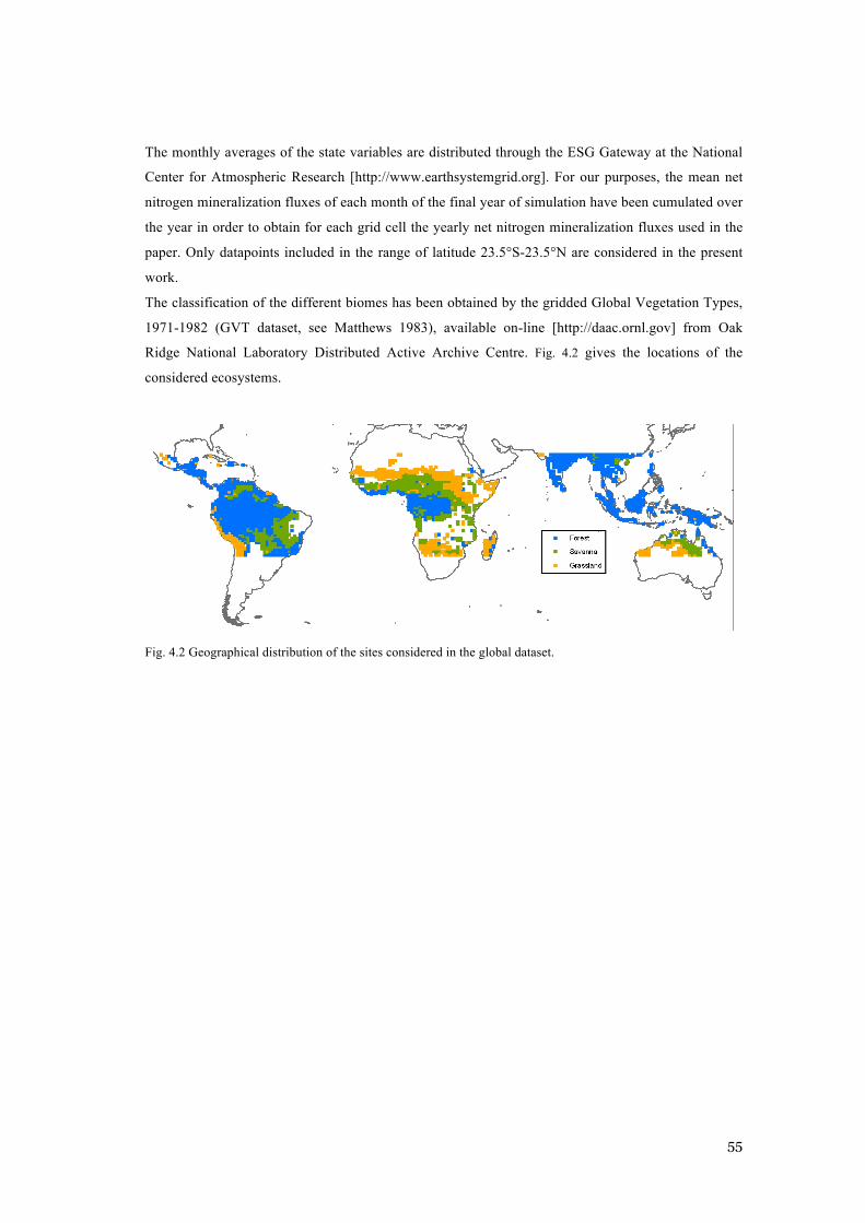
55
The monthly averages of the state variables are distributed through the ESG Gateway at the National
Center for Atmospheric Research [http://www.earthsystemgrid.org]. For our purposes, the mean net
nitrogen mineralization fluxes of each month of the final year of simulation have been cumulated over
the year in order to obtain for each grid cell the yearly net nitrogen mineralization fluxes used in the
paper. Only datapoints included in the range of latitude 23.5°S-23.5°N are considered in the present
work.
The classification of the different biomes has been obtained by the gridded Global Vegetation Types,
1971-1982 (GVT dataset, see Matthews 1983), available on-line [http://daac.ornl.gov] from Oak
Ridge National Laboratory Distributed Active Archive Centre. Fig. 4.2 gives the locations of the
considered ecosystems.
Fig. 4.2 Geographical distribution of the sites considered in the global dataset.
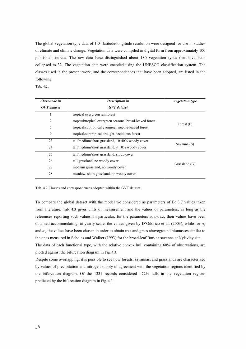
56
The global vegetation type data of 1.0° latitude/longitude resolution were designed for use in studies
of climate and climate change. Vegetation data were compiled in digital form from approximately 100
published sources. The raw data base distinguished about 180 vegetation types that have been
collapsed to 32. The vegetation data were encoded using the UNESCO classification system. The
classes used in the present work, and the correspondences that have been adopted, are listed in the
following
Tab. 4.2.
Class-code in
GVT dataset
Description in
GVT dataset
Vegetation type
1 tropical evergreen rainforest
Forest (F) 2 trop/subtropical evergreen seasonal broad-leaved forest
7 tropical/subtropical evergreen needle-leaved forest
9 tropical/subtropical drought-deciduous forest
23 tall/medium/short grassland, 10-40% woody cover Savanna (S)
24 tall/medium/short grassland, < 10% woody cover
25 tall/medium/short grassland, shrub cover
Grassland (G) 26 tall grassland, no woody cover
27 medium grassland, no woody cover
28 meadow, short grassland, no woody cover
Tab. 4.2 Classes and correspondences adopted within the GVT dataset.
To compare the global dataset with the model we considered as parameters of Eq.3.7 values taken
from literature. Tab. 4.3 gives units of measurement and the values of parameters, as long as the
references reporting such values. In particular, for the parameters a, cT, cG, their values have been
obtained accommodating, at yearly scale, the values given by D’Odorico et al. (2003), while for αT
and αG the values have been chosen in order to obtain tree and grass aboveground biomasses similar to
the ones measured in Scholes and Walker (1993) for the broad-leaf Burkea savanna at Nylsvley site.
The data of each functional type, with the relative convex hull containing 60% of observations, are
plotted against the bifurcation diagram in Fig. 4.3.
Despite some overlapping, it is possible to see how forests, savannas, and grasslands are characterized
by values of precipitation and nitrogen supply in agreement with the vegetation regions identified by
the bifurcation diagram. Of the 1331 records considered ≈72% falls in the vegetation regions
predicted by the bifurcation diagram in Fig. 4.3.
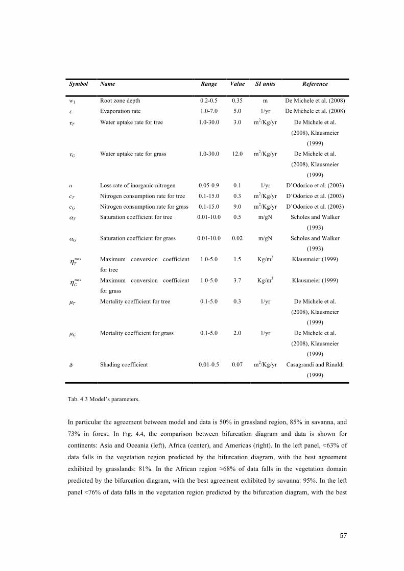
57
Symbol Name Range Value SI units Reference
w1 Root zone depth 0.2-0.5 0.35 m De Michele et al. (2008)
ε Evaporation rate 1.0-7.0 5.0 1/yr De Michele et al. (2008)
τT Water uptake rate for tree 1.0-30.0 3.0 m2/Kg/yr De Michele et al.
(2008), Klausmeier
(1999)
τG Water uptake rate for grass 1.0-30.0 12.0 m2/Kg/yr De Michele et al.
(2008), Klausmeier
(1999)
a Loss rate of inorganic nitrogen 0.05-0.9 0.1 1/yr D’Odorico et al. (2003)
cT Nitrogen consumption rate for tree 0.1-15.0 0.3 m2/Kg/yr D’Odorico et al. (2003)
cG Nitrogen consumption rate for grass 0.1-15.0 9.0 m2/Kg/yr D’Odorico et al. (2003)
αT Saturation coefficient for tree 0.01-10.0 0.5 m/gN Scholes and Walker
(1993)
αG Saturation coefficient for grass 0.01-10.0 0.02 m/gN Scholes and Walker
(1993) maxTη
Maximum conversion coefficient
for tree
1.0-5.0 1.5 Kg/m3 Klausmeier (1999)
maxGη Maximum conversion coefficient
for grass
1.0-5.0 3.7 Kg/m3 Klausmeier (1999)
µT Mortality coefficient for tree 0.1-5.0 0.3 1/yr De Michele et al.
(2008), Klausmeier
(1999)
µG Mortality coefficient for grass 0.1-5.0 2.0 1/yr De Michele et al.
(2008), Klausmeier
(1999)
δ Shading coefficient 0.01-0.5 0.07 m2/Kg/yr Casagrandi and Rinaldi
(1999)
Tab. 4.3 Model’s parameters.
In particular the agreement between model and data is 50% in grassland region, 85% in savanna, and
73% in forest. In Fig. 4.4, the comparison between bifurcation diagram and data is shown for
continents: Asia and Oceania (left), Africa (center), and Americas (right). In the left panel, ≈63% of
data falls in the vegetation region predicted by the bifurcation diagram, with the best agreement
exhibited by grasslands: 81%. In the African region ≈68% of data falls in the vegetation domain
predicted by the bifurcation diagram, with the best agreement exhibited by savanna: 95%. In the left
panel ≈76% of data falls in the vegetation region predicted by the bifurcation diagram, with the best
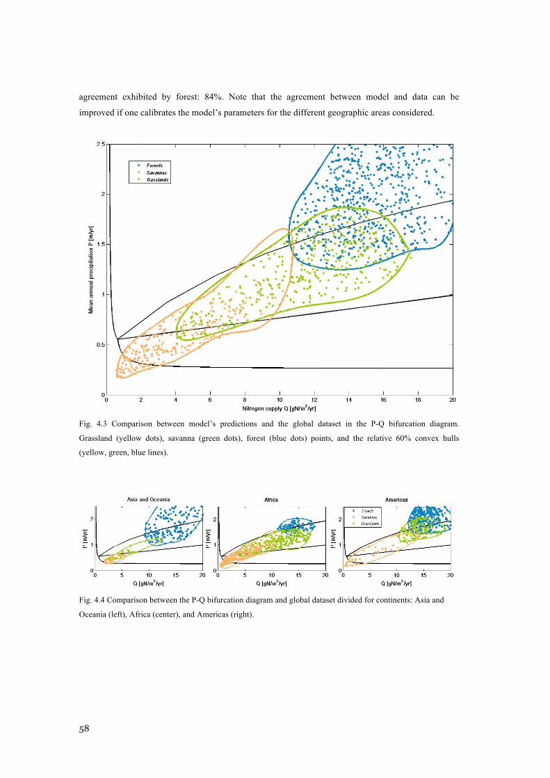
58
agreement exhibited by forest: 84%. Note that the agreement between model and data can be
improved if one calibrates the model’s parameters for the different geographic areas considered.
Fig. 4.3 Comparison between model’s predictions and the global dataset in the P-Q bifurcation diagram.
Grassland (yellow dots), savanna (green dots), forest (blue dots) points, and the relative 60% convex hulls
(yellow, green, blue lines).
Fig. 4.4 Comparison between the P-Q bifurcation diagram and global dataset divided for continents: Asia and
Oceania (left), Africa (center), and Americas (right).
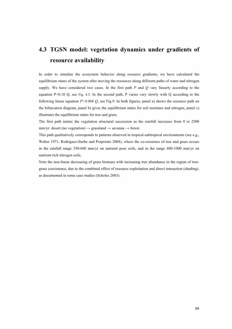
59
4.3 TGSN model: vegetation dynamics under gradients of
resource availability
In order to simulate the ecosystem behavior along resource gradients, we have calculated the
equilibrium states of the system after moving the resources along different paths of water and nitrogen
supply. We have considered two cases. In the first path P and Q vary linearly according to the
equation P=0.18 Q, see Fig. 4.5. In the second path, P varies very slowly with Q according to the
following linear equation P=0.006 Q, see Fig.9. In both figures, panel a) shows the resource path on
the bifurcation diagram, panel b) gives the equilibrium states for soil moisture and nitrogen, panel c)
illustrates the equilibrium states for tree and grass.
The first path mimic the vegetation structural succession as the rainfall increases from 0 to 2500
mm/yr: desert (no vegetation) → grassland → savanna → forest.
This path qualitatively corresponds to patterns observed in tropical-subtropical environments (see e.g.,
Walter 1971, Rodriguez-Iturbe and Porporato 2004), where the co-existence of tree and grass occurs
in the rainfall range 350-600 mm/yr on nutrient poor soils, and in the range 600-1000 mm/yr on
nutrient-rich nitrogen soils.
Note the non-linear decreasing of grass biomass with increasing tree abundance in the region of tree-
grass coexistence, due to the combined effect of resource exploitation and direct interaction (shading),
as documented in some case studies (Scholes 2003).
60
Fig. 4.5 Steady states of tree, grass, soil moisture and mineralized nitrogen along the path P=0.18 Q. Panel a)
shows the resource path on the bifurcation diagram, panel b) gives the equilibrium states for soil moisture and
nitrogen, panel c) illustrates the equilibrium states for tree and grass.
The second path mimics a gradient in soil nitrogen availability, in the middle of the typical savanna
rainfall range. It shows the negative dependence between woody abundance and soil nitrogen supply,
allowing the shift of the system towards a state of higher grass abundance and even the suppression of
the woody layer. Observational support for this result can be found in Sankaran et al. (2008), and for
instance, in the striking difference in tree cover between the granitic (low N) and basaltic (high N)
soils in the Kruger National park in South Africa (Scholes et al. 2003). Typically, this difference has
been ascribed to differences in the fire and herbivory regime, which may still be the case, but this
model result shows that other explanations are possible.
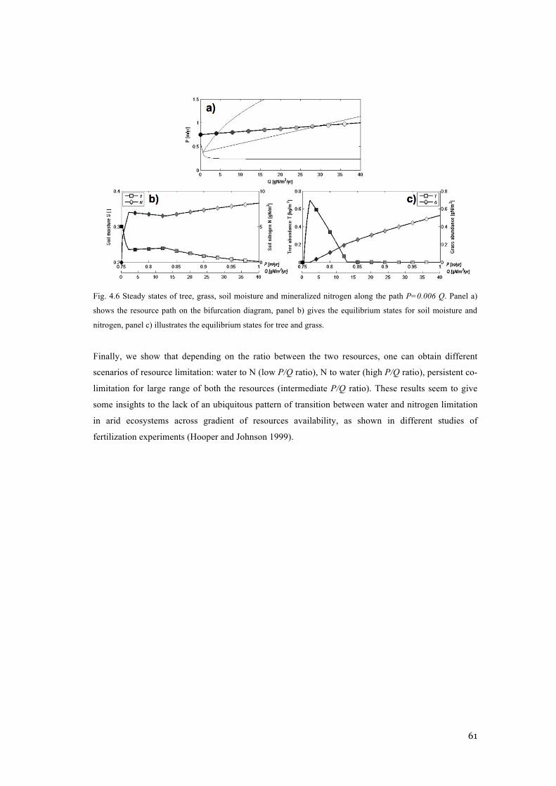
61
Fig. 4.6 Steady states of tree, grass, soil moisture and mineralized nitrogen along the path P=0.006 Q. Panel a)
shows the resource path on the bifurcation diagram, panel b) gives the equilibrium states for soil moisture and
nitrogen, panel c) illustrates the equilibrium states for tree and grass.
Finally, we show that depending on the ratio between the two resources, one can obtain different
scenarios of resource limitation: water to N (low P/Q ratio), N to water (high P/Q ratio), persistent co-
limitation for large range of both the resources (intermediate P/Q ratio). These results seem to give
some insights to the lack of an ubiquitous pattern of transition between water and nitrogen limitation
in arid ecosystems across gradient of resources availability, as shown in different studies of
fertilization experiments (Hooper and Johnson 1999).
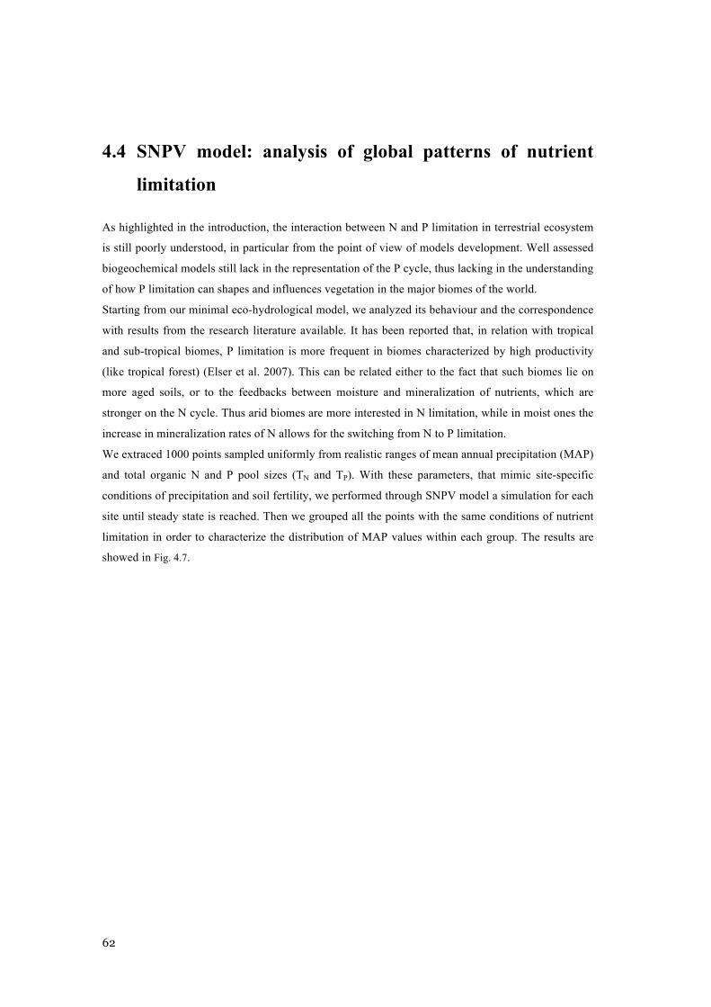
62
4.4 SNPV model: analysis of global patterns of nutrient
limitation
As highlighted in the introduction, the interaction between N and P limitation in terrestrial ecosystem
is still poorly understood, in particular from the point of view of models development. Well assessed
biogeochemical models still lack in the representation of the P cycle, thus lacking in the understanding
of how P limitation can shapes and influences vegetation in the major biomes of the world.
Starting from our minimal eco-hydrological model, we analyzed its behaviour and the correspondence
with results from the research literature available. It has been reported that, in relation with tropical
and sub-tropical biomes, P limitation is more frequent in biomes characterized by high productivity
(like tropical forest) (Elser et al. 2007). This can be related either to the fact that such biomes lie on
more aged soils, or to the feedbacks between moisture and mineralization of nutrients, which are
stronger on the N cycle. Thus arid biomes are more interested in N limitation, while in moist ones the
increase in mineralization rates of N allows for the switching from N to P limitation.
We extraced 1000 points sampled uniformly from realistic ranges of mean annual precipitation (MAP)
and total organic N and P pool sizes (TN and TP). With these parameters, that mimic site-specific
conditions of precipitation and soil fertility, we performed through SNPV model a simulation for each
site until steady state is reached. Then we grouped all the points with the same conditions of nutrient
limitation in order to characterize the distribution of MAP values within each group. The results are
showed in Fig. 4.7.
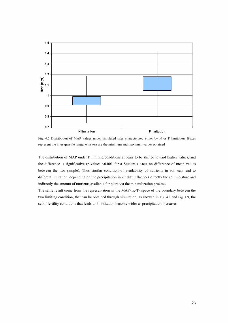
63
Fig. 4.7 Distribution of MAP values under simulated sites characterized either by N or P limitation. Boxes
represent the inter-quartile range, whiskers are the minimum and maximum values obtained
The distribution of MAP under P limiting conditions appears to be shifted toward higher values, and
the difference is significative (p-values <0.001 for a Student’s t-test on difference of mean values
between the two sample). Thus similar condition of availability of nutrients in soil can lead to
different limitation, depending on the precipitation input that influences directly the soil moisture and
indirectly the amount of nutrients available for plant via the mineralization process.
The same result come from the representation in the MAP-TN-TP space of the boundary between the
two limiting condition, that can be obtained through simulation: as showed in Fig. 4.8 and Fig. 4.9, the
set of fertility conditions that leads to P limitation become wider as precipitation increases.
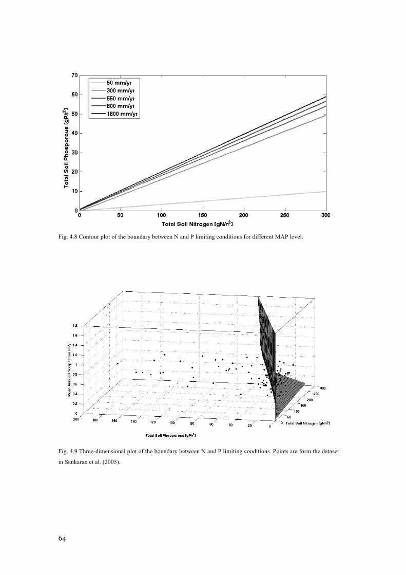
64
Fig. 4.8 Contour plot of the boundary between N and P limiting conditions for different MAP level.
Fig. 4.9 Three-dimensional plot of the boundary between N and P limiting conditions. Points are form the dataset
in Sankaran et al. (2005).
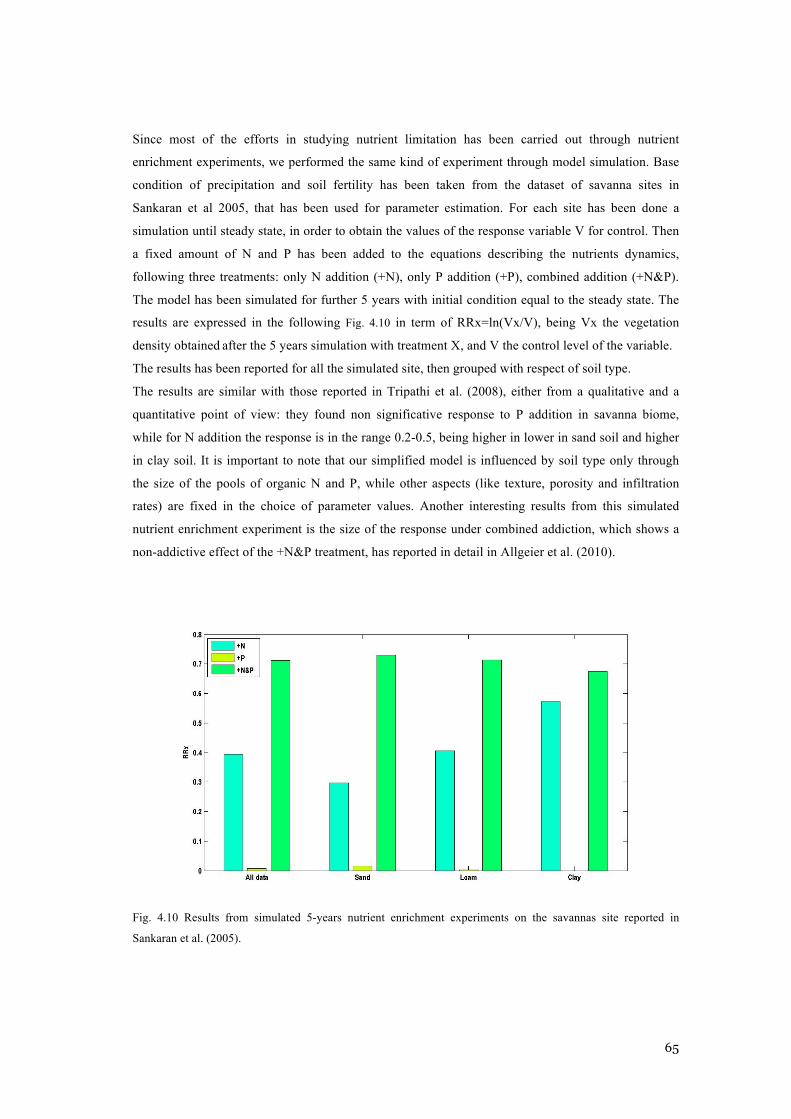
65
Since most of the efforts in studying nutrient limitation has been carried out through nutrient
enrichment experiments, we performed the same kind of experiment through model simulation. Base
condition of precipitation and soil fertility has been taken from the dataset of savanna sites in
Sankaran et al 2005, that has been used for parameter estimation. For each site has been done a
simulation until steady state, in order to obtain the values of the response variable V for control. Then
a fixed amount of N and P has been added to the equations describing the nutrients dynamics,
following three treatments: only N addition (+N), only P addition (+P), combined addition (+N&P).
The model has been simulated for further 5 years with initial condition equal to the steady state. The
results are expressed in the following Fig. 4.10 in term of RRx=ln(Vx/V), being Vx the vegetation
density obtained after the 5 years simulation with treatment X, and V the control level of the variable.
The results has been reported for all the simulated site, then grouped with respect of soil type.
The results are similar with those reported in Tripathi et al. (2008), either from a qualitative and a
quantitative point of view: they found non significative response to P addition in savanna biome,
while for N addition the response is in the range 0.2-0.5, being higher in lower in sand soil and higher
in clay soil. It is important to note that our simplified model is influenced by soil type only through
the size of the pools of organic N and P, while other aspects (like texture, porosity and infiltration
rates) are fixed in the choice of parameter values. Another interesting results from this simulated
nutrient enrichment experiment is the size of the response under combined addiction, which shows a
non-addictive effect of the +N&P treatment, has reported in detail in Allgeier et al. (2010).
Fig. 4.10 Results from simulated 5-years nutrient enrichment experiments on the savannas site reported in
Sankaran et al. (2005).

66
5 CONLUSIONS AND FURTHER
DEVELOPMENTS
This chapter will resume the main results obtained through the analysis of the two eco-hydrological
models developed in the present work. Finally it will be presented some further improvements on the
models that are the object of ongoing research activities.
Relevant works that could act as a premise for such activities will be presented. For each improvement
will be showed the areas in which it could lead to insights in understanding plant-soil interactions in
tropical and subtropical biomes.
One of the main subjects of these ongoing activities are the introduction of the intrinsic stochastic
behaviour of rainfall forcing and soil characteristics, which could be represented respectively as
random processes and random fields. Also the mineralization of nutrients presents a stochastic nature,
since the decay rates of the components of soil organic matter could be modeled in term of proper
probabilitty distributions. Finally, taking into account also the influences of fire and herbivory as
nutrients sinks as sources could improve the reliability of the models and their prediction capability.
67
5.1 Insights from TGSN and SNPV model
As stated in the Introduction, the paucity of reliable data at significative time and spatial scales on
nutrient dynamics requires a theoretical approach in order to highlight the relevant process and to
focus the experimental and modelling effort into proper directions. On the other hand, the extensive
use of explicit models that are not linked to data and observations from different disciplines gives
results that are poorly explicative, leading to contrasting hypothesis that survive in the literature, as
seen in the context of resource competition status. The effort in “filling-the-gap” between different
fields of research is crucial if we want to gain a deep understanding of the complex interactions in the
biosphere.
The idea here is to address the problem through a theoretical approach, using simple dynamical
models as a laboratory to test the behavior of specific ecosystems against data and observations
available.
In particular, the TGSN model focused on the role of competition of plant functional types for
multiple resources from the soil. Two contrasting hypotheses of competition status, which are
supported in the research literature, are discriminated by comparing the predictions of a minimal eco-
hydrological mole against data from measurements of soil fertility, climatology and vegetation density
from various sites in Africa.
In the context of savanna modeling, a great effort has been taken in order to address the competition
between tree and grasses for soil water, however a clear answer about which is the superior competitor
for water is yet to be given. The same argument holds with much more strength when we consider the
competition for soil nitrogen, issue less studied, presenting difficulties connected to the scarcity of
direct and reliable measurements of nitrogen availability at proper spatial and temporal scales, thus
limiting the reliability of explicit models (Botter et al. 2009, Everard et al. 2010 for some recent
examples).
Our analysis suggests that such ecosystems can be viewed in term of coexistence between tree and
grasses permitted by differential strategies adopted by the two dominating functional types with
respect to the most limiting resources, that are water and nitrogen. These differential strategies lead
trees to be the superior competitor for soil nitrogen, while grasses the superior competitor for soil
moisture.
The model’s results are then compared to a global simulated dataset produced by CLM4CN (Oleson et
al. 2010). This can be viewed as a comparison with a quite sophisticated model available in literature,
a spatially distributed land model covering all the earth surface and including biogeochemical cycles
(carbon and nitrogen), vegetation dynamics, land use and river routing (ending with 297 output
variables, compared to the 4 state variables of our minimal model. The comparison shows an
agreement of about 72%.
68
The model’s results exhibit also successions of vegetation structure along gradients of resources, and
in relation to contrasts in soil fertility which match those observed in nature (Hooper and Johnson
1999, Sankaran et al. 2008). Similar results can be seen in Accatino et al. 2010, but translating this
behavior in term of biomass rather than coverage needs the inclusion of nutrients as key factors in
order to capture the non linearity of tree-grass interactions (Scholes 2003).
In a similar way, but starting with an even poorer quantitative description of the processes involved,
the SNPV model tyies to analyze the interaction between hydrological and biogeochemical cycles and
its role in determining pattern of nutrients limitation. The eco-hydrological model has been developed
starting from the equations of soil water balance, nitrogen and phosporous mineralization-
immobilization turnovers. The vegetation dynamics has been represented according to the Liebig’s
law of the minimum, leading to a non-smooth dynamical system.
The resulting pattern of nutrient limitation has qualitative correspondance with observation of such
processe in tropical and subtropical. Simulation of nutrient enrichment on sites with measured values
of resource availability are coherent with meta-analysis of real fertilization studies, despite the
minimality of the model and the parimonious parameterization.
These models and their analysis do not solve the debate between equilibrium and disturbance based
interpretations of biome distribution, even if they try to clarify, at least for savannas ecosytems, the
role of multiple limiting resources in the tree-grass coexistence. Clearly resource competition and
disturbance (such as fire and herbivory) are not mutually exclusive, and confirmation or confutation of
the presented results will require thoughtful experimentation.
5.2 Ongoing activities
The generality of our eco-hydrological approach in addressing specific topic in biomes ecology could
be improved in different ways.
The seasonal and stochastic nature of precipitation and its influence on soil moisture and vegetation
dynamics has been studied in De Michele et al. (2008) and Vezzoli et al. (2008). This approach could
be incorporated in the TGSN model, giving insights in the role of the timing of nutrient uptake and
mineralization, which depend on soil moisture conditions. This is expected to gain relevance in the
arid end of the sub-tropical catena, as showed in Scholes et al. 1999 and Williams et al. 2008. An
explicit seasonal representation could allow for a comparison with observations of asyncrony between
precipitation and nitrogen mineralization, which is documented in Augustine and McNaugthon (2004)
in some arid savannas and it is thinked to be peculiar in subtropical rather than temperate ecosystems.
In the same way, the relevance of disturbances like fire and herbivory in savannas has been showed in
De Michele et al. (2011). Taking into account that effect could improve the results of both TGSN and

69
SNPV model, since those disturbances in turn influence also the nutrient cycling, being either losses
(fire) and sources (herbivory) for nutrients.
Another ongoing activity deal with the representation through random fields of the spatial distribution
of soil fertility indexes, such as the size of nutrient pools in soil organic matter. This approach could
lead to downscaling procedure in order to fill the gap between the spatial scale of global
biogeochemical models (>50 km) and those of measurements from the field (<300 m).
An inherent source of uncertanty related to the nutrient cycling come from the mineralization process.
The first order kinetics adopted in the SNPV model could be improved by representing the organic
matter as a continuum of components characterized by a range of decomposition rates according to
proper probability distributions. This approach has been effectively used by Rothman and Forney
(2007) in modeling the decomposition of organic matter in oceanic sediments.
70
References
Acary V, Brogliato B, 2009. Numerical Methods for Nonsmooth Dynamics. Application in Mechanics
and Electronics. Springer.
Accatino F, De Michele C, Vezzoli R, Donzelli D, Scholes RJ, 2010. Tree–grass co-existence in
savanna: interactions of rain and fire. Journal of Theoretical Biology, 267, 235–242.
Allgeier JE, Rosemond AD and Layman CA, 2010. The frequency and magnitude of non-additive
responses to multiple nutrient enrichment. Journal of Applied Ecology, 48 (1).
Augustine DJ and McNaughton SJ, 2004. Temporal Asynchrony in Soil Nutrient Dynamics and Plant
Production in a Semiarid Ecosystem. Ecosystems, 7 (8), 829-840.
Bond WJ and Keeley JE, 2005. Fire as a global ‘herbivore’: the ecology and evolution of flammable
ecosystems. Trends in Ecology and Evolution, 20 (7), 387-394.
Botter G, Daly E, Porporato A, Rodriguez-Iturbe I, Rinaldo A, 2008. Probabilistic dynamics of soil
nitrate: coupling of ecohydrological and biogeochemical processes. Water Resources Research, 44(3),
W03416.
Breman H, de Wit CT, 1983. Rangeland productivity and exploitation in the Sahel. Science,
221(4618), 1341–1347.
Bucini G, Hanan NP, 2007. A continental-scale analysis of tree cover in African savannas. Global
Ecology and Biogeography, 16(5), 593-605.
71
Casagrandi R, Rinaldi S, 1999. A minimal model for forest fire regimes. The American Naturalist,
153, 527–539.
De Michele C, Accatino F, Vezzoli R and Scholes RJ, 2011. Savanna domain in the herbivores-fire
parameter space exploiting a tree-grass-soil water dynamic model. Journal of Theoretical Biology,
289, 74-82.
De Michele C, Vezzoli R, Pavlopulous H, Scholes RJ, 2008. A minimal model of soil water-
vegetation interactions forced by stochastic rainfall in water-limited ecosystems. Ecological Modeling,
212, 397–407.
Dhooge A, Govaerts W, Kuznetsov YA, Mestrom W, Riet AM, Sautois B, 2006. Matcont and Cl-
Matcont: Continuation toolboxes in Matlab. Utrecht University, The Netherlands.
D'Odorico P, Laio F, Porporato A, Rodriguez-Iturbe I, 2003. Hydrologic controls on soil carbon and
nitrogen cycles. II. A case study. Advances in Water Resources, 26(1), 59-70.
D'Odorico P, Laio F, Ridolfi L, 2006. A probabilistic analysis of fire-induced tree-grass coexistence in
savannas. American Naturalist, 167(3) E79-E87.
Dybzinski R, Tilman D, 2007. Resource use patterns predict long-term outcomes of plant competition
for nutrients and light. American Naturalist, 170, 305-318.
Elser JJ, Bracken MES, Cleland EE, Gruner DS, Harpole WS, Hillebrand H, Ngai JT, Seabloom EW,
Shurin JB, Smith JE, 2007. Global analysis of nitrogen and phosphorus limitation of primary
producers in freshwater, marine and terrestrial ecosystems. Ecology Letters, 10 (12), 1135–1142.
Everard K, Seabloom EW, Harpole WS, de Mazancourt C, 2010. Plant water use affects competition
for nitrogen: why drought favors invasive species in California. American Nauralist, 175, 85-97.
Frost PG, Medina E, Menaut JC, Solbrig O, Swift M, Walker BH (eds). 1986. Response of savannas
to stress and disturbance. Biology International Special Issue 10, IUBS, Paris.
72
Gebauer RLE, Ehleringer JR, 2000. Water and nitrogen uptake patterns following moisture pulses in a
cold desert community. Ecology, 81(5), 1415–1424.
Gebauer RLE, Schwinning S, Ehleringer JR, 2002. Interspecific competition and resource pulse
utilization in a cold desert community. Ecology, 83(9), 2602–2616.
Gleeson SK, Tilman D, 1992. Plant allocation and the multiple limitation hypothesis. American
Naturalist, 139 (6), 1322-1343.
Hanan NP, Sea WB, Dangelmayr G, Govender N, 2008. Do fires in savannas consume woody
biomass? A comment on approaches to modeling savanna dynamics. American Naturalist, 171(6),
851-856.
Harpole WS, Suding KN, 2011. A test of the niche dimension hypothesis in an arid annual grassland.
Oecologia, 166:197-205.
Harpole WS, Tilman D, 2007. Grassland species loss resulting from reduced niche dimension. Nature,
446:791-793.
Higgins SI, Scheiter S, Sankaran M, 2010. The stability of African savannas: insights from the
indirect estimation of the parameters of a dynamic model. Ecology, 91(6), 1682–1692.
Hooper DU, Johnson L, 1999. Nitrogen limitation in dryland ecosystems: responses to geographical
and temporal variation in precipitation. Biogeochemistry 46, 247–293.
Jansson SL and Persson J, 1982. Mineralization and immobilization of soil nitrogen. In: Nitrogen in
Agricultural Soils. Stevenson FJ (ed.). Agron. Monogr. 22. American Society of Agronomy, Madison,
WI.
Jenkinson DS, Andrew SPS, Lynch JM, Goss MJ and Tinker PB, 1990. The Turnover of Organic
Carbon and Nitrogen in Soil. Phil. Trans. R. Soc. Lond. B, 329 (1255), 361-368.
73
Keymer JE, Fuentes MA, Marquet PA, 2008. Diversity emerging: from competitive exclusion to
neutral coexistence in ecosystems. Santa Fe Institute Working Paper, 08-03-008.
Klausmeier CA, 1999. Regular and irregular patterns in semiarid vegetation. Science, 284, 1826-1828.
Kraaij T, Ward D, 2006. Effects of rain, nitrogen, fire and grazing on tree recruitment and early
survival in bush-encroached savanna, South Africa. Plant Ecology, 186, 235–246.
Kuznetsov YA, 1995. Elements of applied bifurcation theory. Springer, New York.
Larcher W, 2003. Physiological plant ecology: ecophysiology and stress physiology of functional
groups (4th ed.). Springer, New York.
Marschner P and Rengel Z (eds.), 2007. Nutrient Cycling in Terrestrial Ecosystems. Springer-Verlag
Berlin Heidelberg.
Matthews E, 1983. Global vegetation and land use: new high-resolution data bases for climate studies.
Journal of Climate and Applied Meteorology, 22, 474–487.
Meyer KM, Wiegand K, Ward D, 2009. Patch dynamics integrate mechanisms for savanna tree–grass
coexistence. Basic and Applied Ecology, 10, 491–499.
Oleson KW, Lawrence DM, Bonan GB, Flanner MG, Kluzek E, Lawrence PJ, Levis S, Swenson SC,
Thornton PE, Dai A, Decker M, Dickinson R, Feddema J, Heald CL, Hoffman F, Lamarque JF,
Mahowald N, Niu GY, Qian T, Randerson J, Running S, Sakaguchi K, Slater A, Stockli R, Wang A,
Yang ZL, Zeng Xi, Zeng Xu, 2010. Technical Description of version 4.0 of the Community Land
Model (CLM). NCAR Technical Note NCAR/TN-478+STR, National Center for Atmospheric
Research, Boulder, CO.
Olff H, Ritchie ME, Prins HHT, 2002. Global environmental controls of diversity in large herbivores.
Nature, 415(6874), 901-904.
74
Parton WJ, Schimel DS, Cole CV and Ojima DS, 1987. Analysis of Factors Controlling Soil Organic
Matter Levels in Great Plains Grasslands. Soil Science Society of America Journal, 51 (5), 1173-1179.
Piiroinen PT, Kuznetsov YA, 2008. An event-driven method to simulate Filippov systems with
accurate computing of sliding motions. ACM Transactions on Mathematical Software, 34 (3).
Press WH, Teukolsky SA, Vetterling WT, Flannery BP, 1992. Numerical Recipes in C: The Art of
Scientific Computing, Second Edition. Cambridge University Press.
Ricklefs RE, 2008. The economy of nature. WH Freeman & Co.
Rodriguez-Iturbe I, Porporato A, 2004. Ecohydrology of water-controlled ecosystems: soil moisture
and plant dynamics. Cambridge University Press, Cambridge, UK.
Rothman Dh and Forney DC, 2007. Physical Model for the Decay and Preservation of Marine
Organic Carbon. Science, 316 (5829), 1325-1328.
Rudolf B, Becker A, Schneider U, Meyer-Christoffer A, Ziese M, 2010. GPCC Status Report July
2010.
Rudolf B, Schneider U, 2005. Calculation of Gridded Precipitation Data for the Global Land-Surface
using in-situ Gauge Observations. Proceedings of the 2nd Workshop of the International Precipitation
Working Group IPWG, Monterey October 2004, EUMETSAT.
Salvadori G, Kottegoda N, De Michele C, Rosso R, 2007. Extremes in nature: an approach using
Copulas. Springer-Verlag New York Inc., New York, NY.
Sankaran M, Hanan NP, Scholes RJ, Augustine DJ, Cade BS, Gignoux J, Higgins SI, Le Roux X,
Ludwig F, Ardo J, Banyikwa F, Bronn A, Bucini G, Caylor KK, Coughenour MB, Diouf A, Ekaya W,
Feral CJ, February EC, Frost PGH, Hiernaux P, Hrabar H, Metzger KL, Prins HHT, Ringrose S, Sea
W, Tews J, Worden J, Zambatis N, 2005. Determinants of woody cover in African savannas. Nature,
438(7069), 846-849.
75
Sankaran M, Ratnam J, Hanan NP, 2008. Woody cover in African savannas: the role of resources, fire
and herbivory. Global Ecology and Biogeography, 17, 236-245.
Shaffers AP, 2000. In situ annual nitrogen mineralization predicted by simple soil properties and
short-period field incubation. Plant and Soil, 221, 205-219.
Scholes MC, Martin R, Scholes RJ, Parsons D and Winstead E, 1999. NO and N2O emissions from
savanna soils following the first simulated rains of the season. Nutrient Cycling in Agroecosystems, 48
(1-2), 115-122.
Scholes RJ, Walker BH, 1993. An African Savanna: Synthesis of the Nylsvley Study. Cambridge
University Press, Cambridge, UK.
Scholes, RJ, Hall DO, 1996. The carbon budget of tropical grasslands, savannas and woodlands. In:
A.I. Breymeyer, D.O. Hall, J.M. Melillo & G.I. Agren (eds) Global Change: Effects on Coniferous
Forests and Grasslands. SCOPE 1996. New York: John Wiley, 69-100.
Scholes RJ, Dowty PR, Caylor K, Parsons DAB, Frost PGH, Shugart HH, 2002. Trends in savanna
structure and composition along an aridity gradient in the Kalahari. Journal of Vegetation Science,
13(3), 419-428.
Scholes RJ, 2003. Convex relationships in ecosystems containing mixtures of trees and grass.
Environmental and Resource Economics, 26, 559–574.
Scifres CJ, Mutz JL, Whitson RE, Drawe DL, 1982. Interrelationships of huisache canopy cover with
range forage on the coastal prairie. Journal of Range Management, 35, 558-562.
Solbrig O, Medina E, Silva J, 1996. Biodiversity and tropical savanna properties: a global view. In:
Mooney, H., Cushman, J., Medina, E., Sala, O., Schulze., E. (Eds.), Functional Role of Biodiversity: a
Global Prospective. John Wiley and Sons Ltd., 185–211.
Teague WR, Smit GN, 1992. Relations between woody and herbaceous components and the effects of
bush-clearing in southern African savannas. Journal of the Grasslands Society Southern Africa, 9, 60-
71.
76
Tilman D, 1982. Resource Competition and Community Structure. Monographs in Population
Biology, Princeton University Press.
Tilman D, 1985. The resource-ratio hypothesis of plant succession. American Naturalist, 125 (6), 827-
852.
Tripathi SK, Kushwaha CP and Singh KP, 2008. Tropical forest and savanna ecosystems show
differential impact of N and P additions on soil organic matter and aggregate structure. Global Change
Biology, 14, 2572–2581.
Vezzoli R, De Michele C, Pavlopoulos H, Scholes RJ, 2008. Dryland ecosystems: The coupled
stochastic dynamics of soil water and vegetation and the role of rainfall seasonality. Physical Review
E, 77 (5).
Walter H, 1971. Ecology of Tropical and Subtropical Vegetation. Oliver and Boyd, Edinburgh, UK.
Wang L, D’Odorico P, Reies L, Macko SA, 2010. Patterns and implications of plant-soil δ13C and
δ15N values in African savanna ecosystems, Quaternary Research, 73, 77–83.
Wang L, D’Odorico P, O’Halloran Reies L, Caylor K, Macko S, 2010. Combined effects of soil
moisture and nitrogen availability variations on grass productivity in African savannas. Plant Soil,
328, 95–108.
Whittaker RH, 1975. Community and ecosystems. McMillan, New York.
Williams CA, Hanan N, Scholes RJ and Kutsch W, 2009. Complexity in water and carbon dioxide
fluxes following rain pulses in an African savanna. Oecologia, 161 (3), 469-480.