CHAPTER 10

Ecological modeling of short-term plant community dynamics under grazing with and without disturbance

L.F.M. Fresco, H.P.M. van Laarhoven, M.J.J.E. Loonen & T. Moesker

Detailed contents 1. Introduction ..... . ......... ,................ 149

1.1 Models of plant community- and ecosystem-dynamics... .. .. . .. ..................... 149

1.2 The use of an explanatory model ........... 150 1.3 The modeling of disturbance. . . . . . . . . . . . . .. 151 1.4 The aims of modeling short-term plant com­

munity dynamics . . . . . . . . . . . . . . . . . . . . . . . .. 152 2. Description of the model 'EGRAS' . .. . . . . . . ... .. 153

2.1 GeneraL............................ ... 153 2.2 Growth and death. . . . . . . . . . . . . . . . . . . . .. 154 2.3 Grazing.. . ................. .......... 155 2.4 Abiotic factors. . . . . . . . . . . . . . . . . . . . . . . . . .. 156

1. Introduction

1.1 Models of plant community- and ecosystem­dynamics

A simulation model is a simplified presentation of a system in the real world around us, where this system is a perceived -limited- part of reality. The user determines the system with respect to his own purposes and to the natural structure of the real system (Penning de Vries, 1984). The identi­fication of the system involves (i) the scale, in­duding patch size (spatial size), the time steps plus duration and organization level, (ii) the va­riables to be explained (e.g. vegetation dynamics, animal behaviour, meat production, forage avail­ability), (iii) the 'independent' variables and pa­rameters, the use of which is determined by orga­nization level and a prior insight of the user. It is important that the model should be 'open', Le.

J. van Andel et aI., (eds.). Disturbance in Grasslands. ISBN 90-6193-640-3. © 1987. Dr W. Junk Publishers. Dordrecht. Printed in the Netherlands.

2.5 Simulations of a sequence of seasons. . . . . . . . 157 2.6 Disturbance.......... ........ ......... 158

3. Results. . . . . . . . . . . . . . . . . . . . . .. .............. 158 4. Discussion . . . . . . .. ........... .............. 160,

4.1 Evaluation of the simulation approach.. ... .. 161 4.2 The sufficiency of the model. . . . . . . . . . . . . .. 162 4.3 The use of simulating disturbance .......... 162

Acknowledgements ...................... ...... 163 References. . . . . . . . . . . . . . . . . . . . . . . . . . . . . . . . . 163 Appendix. . . . . . . . . . . . . . . . . . . . . . . . . . . . . . . . . . . . .. 164 1. Procedures concerning growth and death. . . . . . . .. 164 2. Procedures concerning grazing. . . . . . . . . . . . . . . . 165 3. Procedures concerning abiotic factors. . . . . . . . . . .. 165

there is opportunity to include variables which later appear to be important.

The decision as to which type of model is to be built depends mainly on the aims of the project. In the context of vegetation and landscape re­search these aims can either be to predict the changes to be expected or to understand the mechanisms causing these changes (= explana­tion). In the first case it is a primary requirement that the model and the simulation programme are widely applicable. In the second case, i.e. causal­analytical models, this generalization follows from the spatial and temporal dimensions of the real system that was initially chosen to collect data from. This model starts with a theoretical consideration of the internal structure of the sys­tem. In such models a sequence of steps, i.e. building the model, writing the programme, exec­uting the simulation, validating the parameters, analyzing the sensitivity of the model, may be re­

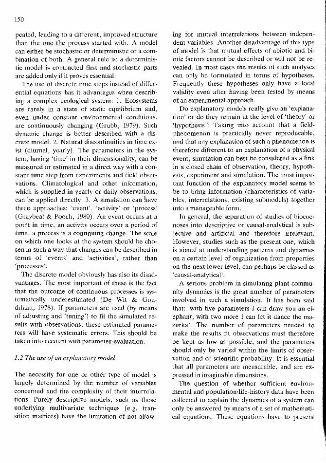
150

peated, leading to a different, improved structure than the one,Jhe process started with. A model can either be stochastic or deterministic or a com­bination of both. A general rule is: a determinis­tic model is contructed first and stochastic parts are added only if it proves essential.

The use of discrete time steps instead of differ­ential equations has it advantages when describ­ing a complex ecological system: 1. Ecosystems are rarely in a state of static equilibrium and, even under constant environmental conditions, are continuously changing (Grubb, 1979). Such dynamic change is better described with a dis­crete model. 2. Natural discontinuities in time ex­ist (diurnal, yearly). The parameters in the sys­tem, having 'time' in their dimensionality, can be measured or estimated in a direct way with a con­stant time step from experiments and field obser­vations. Climatological and other information, which is supplied in yearly or daily observations, can be applied directly. 3. A simulation can have three approaches: 'event', 'activity' or 'process' (Graybeal & Pooch, 1980). An event occurs at a point in time, an activity occurs over a period of time, a process is a continuing change. The scale on which one looks at the system should be cho­sen in such a way that changes can be described in terms of 'events' and 'activities', rather than 'processes' .

The discrete model obviously has also its disad­vantages. The most important of these is the fact that the outcome of continuous processes is sys­tematically underestimated (De Wit & Gou­driaan, 1978). If parameters are used (by means of adjusting and 'tuning') to fit the simulated re­sults with observations, these estimated parame­ters will have systematic errors. This should be taken into account with parameter-evaluation.

1.2 The use ofan explanatory model

The necessity for one or other type of model is largely determined by the number of variables concerned and the complexity of their interrela­tions. Purely descriptive models, such as those underlying multivariate techniques (e.g. tran­sition matrices) have the limitation of not allow­

ing for mutual interrelations between indepen­dent variables. Another disadvantage of this type of model is that mutual effects of abiotic and bi­otic factors cannot be described or will not be re­vealed. In most cases the results of such analyses can only be formulated in terms of hypotheses. Frequently these hypotheses only have a local validity even after having been tested by means of an experimental approach.

Do explanatory models really give an 'explana­tion' or do they remain at the level of 'theory' or 'hypothesis'? Taking into account that a field­phenomenon is practically never reproducable, and that any explanation of such a phenomenon is therefore different to an explanation of a physical event, simulation can best be considered as a link in a closed chain of observation, theory, hypoth­esis, experiment and simulation. The most impor­tant function of the explanatory model seems to be to bring information (characteristics of varia­bles, interrelations, existing submodels) together into a manageable form.

In general, the separation of studies of biocoe­noses into descriptive or causal-analytical is sub­jective and artificial and therefore irrelevant. However, studies such as the present one, which is aimed at understanding patterns and dynamics on a certain level of organization from properties on the next lower level, can perhaps be classed as 'causal-analytical' .

A serious problem in simulating plant commu­nity dynamics is the great number of parameters involved in such a simulation. It has been said that: 'with five parameters I can draw you an el­ephant, with two more I can let it dance the ma­zurka'. The number of parameters needed to make the results fit observations must therefore be kept as low as possible, and the parameters should only be varied within the limits of obser­vation and of scientific probability. It is essential that all parameters are measurable, and are ex­pressed in imaginable dimensions.

The question of whether sufficient environ­mental and population/life-history data have been collected to explain the dynamics of a system can only be answered by means of a set of mathemati­cal equations. These equations have to present

151

ecological reality as well as possible, given the necessary simplifications. The set of equations must be structured usually in a systems-flow-di­agram. This constitutes the modeL This model must be translated into a computer language and can than be used for a simulation. The initial state of a simulation is of primary importance, it has to consist of real (observed) values. If the results of the simulation are consistent with observed dy­namics, then it may represent reality.

1.3 The modeling ofdisturbance

Disturbance can be simulated by constructing a mathematical model of a system, and then sub­jecting the model to events, that can be regarded as a disturbance, with respect to that system, tak­ing into ac<;ount the relevant scale (spatial, tem­poral, integration level). The word 'disturbance' should only be used with reference to a given sys­tem (or family of systems) and a given scale. For example, grazing is certainly a disturbance for an individual leaf, or in most cases an inidividual plant. It is also a disturbance for a grassland com­munity just taken into grazing, but not for a com­munity after a couple of years of grazing.

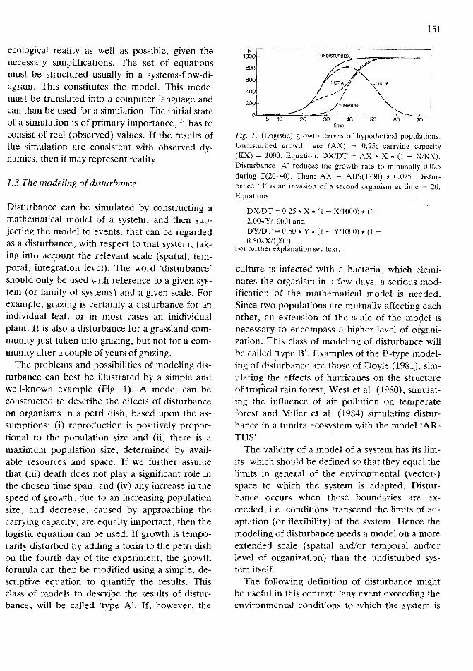
The problems and possibilities of modeling dis­turbance can best be illustrated by a simple and well-known example (Fig. 1). A model can be constructed to describe the effects of disturbance on organisms in a petri dish, based upon the as­sumptions: (i) reproduction is positively propor­tional to the population size and (ii) there is a maximum population size, determined by avail­able resources and space. If we further assume that (iii) death does not playa significant role in the chosen time span, and (iv) any increase in the speed of growth, due to an increasing population size, and decrease, caused by approaching the carrying capacity, are equally important, then the logistic equation can be used. If growth is tempo­rarily disturbed by adding a toxin to the petri dish on the fourth day of the experiment, the growth formula can then be modified using a simple, de­scriptive equation to quantify the results. This class of models to describe the results of distur­bance, will be called 'type N. If, however, the

N 1000 UNDISTURBED

800 .pP-;to

600 v-/ /"DIST.A,,.f· ~'ST.e

400

200

0 5 10 20

~~//""",,~ /

/-INVADER .-./'

30 40

\ "

50

'-... 60 70

time

Fig. 1. (Logistic) growth <-'urves of hypothetical populations. Undisturbed growth rate (AX) = 0.25; carrying capacity (KX) = 1000. Equation: DXlDT AX * X * (1 - XlKX). Disturbanee 'A' reduces the growth rate to minimally 0.025 during T(20-40). Than: AX = ABS(T-30) * 0.025. Distur­bance 'B' is an invasion of a second organism at time 20. Equations:

DXlDT 0.25 * X * (1 Xl10(0) * (1 -­2.00* Y/1000) and DYIDT = 0.50 * Y * (1 - Y/lOOO) * (1 ­0.50*Xl1000).

For further e1planation see text.

culture is infected with a bacteria, which elemi­nates the organism in a few days, a serious mod­ification of the mathematical model is needed. Since two populations are mutually affecting each other, an extension of the scale of the mogel is necessary to encompass a higher level of organi­zation. This class of modeling of disturbance will be called 'type B'. Examples of the B-type model­ing of disturbance are those of Doyle (1981), sim­ulating the effects of hurricanes on the structure of tropical rain forest, West et aL (1980), simulat­ing the influence of air pollution on temperate forest and Miller et aL (1984) simulating distur­bance in a tundra ecosystem with the model 'AR­TUS'.

The validity of a model of a system has its lim­its, which should be defined so that they equal the limits in general of the environmental (vector-) space to which the system is adapted. Distur­bance occurs when these boundaries are ex­ceeded, i.e. conditions transcend the limits of ad­aptation (or flexibility) of the system. Hence the modeling of disturbance needs a model on a more extended scale (spatial and/or temporal and/or level of organization) than the undisturbed sys­tem itself.

The following definition of disturbance might be useful in this context: 'any event exceeding the environmental conditions to which the system is

152

is adapted'. Disturbance is not identical to unpre­dictable variation of a normally variable factor to which variation a system is adapted. Every factor in a system has its own 'predictable unpredictabil­ity'. Terms like 'adaptation to disturbance' or 'continuous disturbance' are not useful. Each sys­tem has its own autogenic dynamics: short-term and long-term, random, cyclic and/or directed (succession). After a system has been disturbed, it no longer exists in its previous form as it has been replaced by a different system with its own dynamics but, after a certain period of time, con­vergent suceession may cause the disturbed and the 'undisturbed systems to become identical. The classification 'disturbance-dependent system' can only be applied to the instable, temporarily exist­ing situation, following a disturbance.

1.4 The aims of modeling short-term plant com­munity dynamics

The understanding and causal explanation of an ecosystem or plant community requires' knowl­edge of 'the species life-history and physiological characteristics which determine, to a large ex­tent, potential population responses to the chang­ing competitive environment' (Peet & Chris­tensen, 1980). Ellenberg (1954) argued that: ' ... questions came up with respect to the causes of these strict relations (between the mosaic of plant communities and environmental condi­tions). These questions can be answered ~y three supplementary means: (i) quantitative compari­son of numerous communities and their habitats, (ii) quantitative analysis of relevant environmen­tal variables and of characteristics and perfor­mance of plants in their own habitats, (iii) experi­mental studies under more or less simplified con­ditions'. The second and third of these can be achieved more succesfully with the help of an ex­planatory model.

An explanatory model of plant community dy­namics must contain characteristics of the species present, including their repsonses to the relevant environmental factors. Interference between spe­cies populations has to be included in such a model, which has to separate competition for dif­

disturb.

potential invaders ... 'sp.N+1 sp,N+2--sp.N+K

r--------------l I interference I I~ I

: sp.1Is~----~sp,N] :

:~'~ : I iphysiological relations II . I

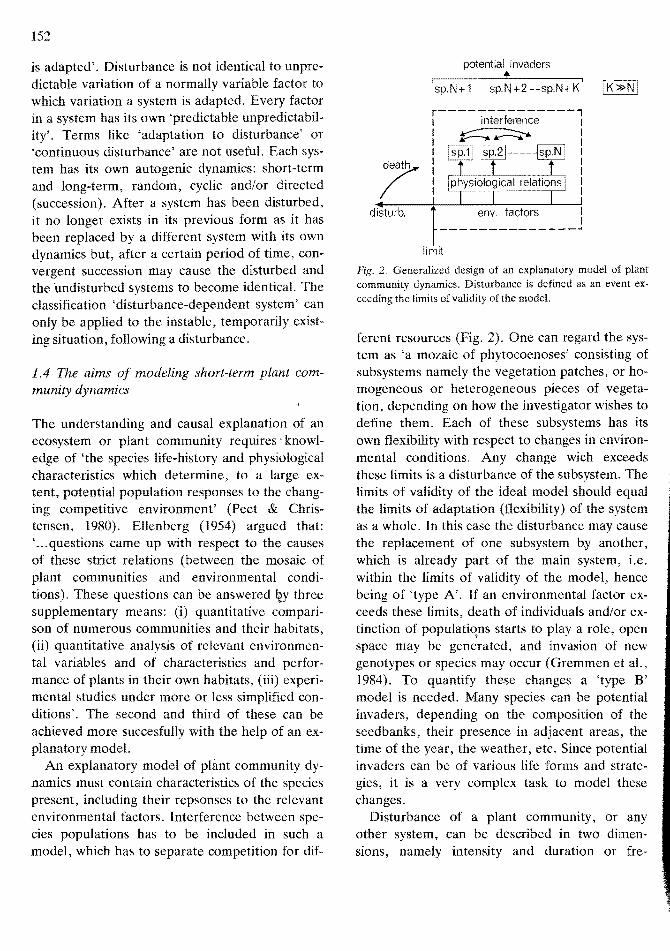
Fig. 2, Generalized design of an explanatory model of plant community dynamies. Disturbance is defined as an event ex­ceeding the limits of validity of the model.

ferent resources (Fig. 2). One can regard the sys­tem as 'a mozaic of phytocoenoses' consisting of subsystems namely the vegetation patches, or ho­mogeneous or heterogeneous pieces of vegeta­tion, depending on how the investigator wishes to define them. Each of these subsystems has its own flexibility with respect to changes in environ­mental conditions. Any change wich exceeds these limits is a disturbance of the subsystem. The limits of validity of the ideal model should equal the limits of adaptation (flexibility) of the system as a whole. In this case the disturbance may cause the replacement of one subsystem by another, which is already part of the main system, i.e. within the limits of validity of the model, hence being of 'type A'. If an environmental factor ex­ceeds these limits, death of individuals and/or ex­tinction of populatiqns starts to playa role, open space may be generated, and invasion of new genotypes or species may occur (Gremmen et aI., 1984). To quantify these changes a 'type B' model is needed. Many species can be potential invaders, depending on the composition of the seedbanks, their presence in adjacent areas, the time of the year, the weather, etc. Since potential invaders can be of various life forms and strate­gies, it is a very complex task to model these changes.

Disturbance of a plant community, or any other system, can be described in two dimen­sions, namely intensity and duration or fre­

153

quency. The time dimension of disturbance has not been covered in this study. Although, in most cases, disturbance will cause destruction of living phytomass or accumulated detritus (Grime, 1979; Reiners, 1983), it is better that this effect is not included in a definition.

In spite of the problems of simulating distur­bance, such an excercise is useful, since it may give the user an idea of the trends and general patterns, that are likely to occur. It is also an ex­cellent method to test the basic model and to find its weak spots and errors. This kind of simulation will only be predictive in the very short term. In­ductive models, based on numerous observations, will be more effective for ldng-term prediction.

2. Description of the model 'EGRAS'

2.1. General

The model 'EGRAS' ('Ecological Grassland Sim­ulator') is concerned with a section of the former Lauwers Sea, which was a part of the Wadden Sea (in the north of the Netherlands), which was embanked in 1969. The actual area involved ('Schildhoek en Pampusplaat') is approximately 200 ha and was designated a feeding area for win­tering and transmigrating wild fowl in 1979. How­ever, this aim was endangered with the increasing amount of litter and standing dead material and increasing dominance of Agrostis stoloni/era, es­pecially in the dryer parts of the area. Therefore, since 1982, the area has been grazed by young cattle at a stocking rate of about 1 animal per hec­tare. The cows enter the area annually in early June and leave it in October. A large exclosure has been established for the purpose of scientific research. Data concerning vegetational cbanges, herbage accumulation and herbage removal by cattle and water fowl and the changing (desalinat­ing) abiotic environment have been published (Joenje, 1978, 1979, 1982). Other information concerning growth characteristics and mutual competitive ability of some plant species, was col­lected in the cause of this study.

The aim of this project was to develop a model

THE OTHER PL. *1 SPECIES

ADJACENT SITES

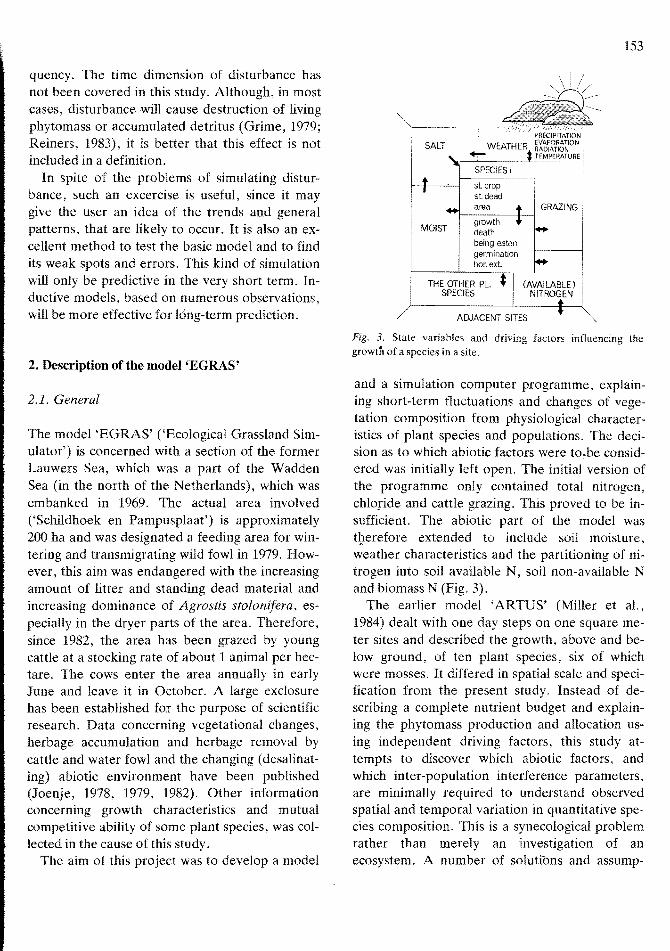
Fig. 3. State variables and driving factors influencing the growth of a species in a site.

and a simulation computer programme, explain­ing short-term fluctuations and changes of vege­tation composition from physiological character­istics of plant species and popUlations. The deci­sion as to which abiotic factors were to.be consid­ered was initially left open. The initial version of the programme only contained total nitrogen, chloride and cattle grazing. This proved to be in­sufficient. The abiotic part of the model was tJ;terefore extended to include soil moisture, weather characteristics and the partitioning of ni­trogen into soil available N, soil non-available N and biomass N (Fig. 3).

The earlier model 'ARTUS' (Miller et aI., 1984) dealt with one day steps on one square me­ter sites and described the growth, above and be­low ground, of ten plant species, six of which were mosses. It differed in spatial scale and speci­fication from the present study. Instead of de­scribing a complete nutrient budget and explain­ing the phytomass production and allocation us­ing independent driving factors, this study at­tempts to discover which abiotic factors, and which inter-popUlation interference parameters, are minimally required to understand observed spatial and temporal variation in quantitative spe­cies composition. This is a synecological problem rather than merely an investigation of an ecosystem. A number of solutions and assump­

154

CONDITION 1I species 1 species2 un ·species5 nit'2ge.rl chloride moisture

CONDITION I

.ST.CROP .ST.DEAD .AREA .%OAMAGE

.SlCROP

.$1: DEAD

.AREA

.%DAMAGE

_TOTAL .CONe. IN .LEVEL .AVAILABLE SOIL WATER .IN BIOMASS O.10cm

• WTAL .CONe. IN .LEVEL .AVAILABLE SOIL WATER .IN BIOMASS O.IOcm

KN.M.I. weather rep.

WEATHER (temp. light

precip. c\lap,)

GROWTH PARAMETERS

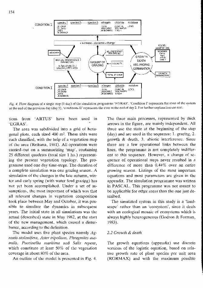
Fig. 4. Flow diagram of a single step (1 day) of the simulation programme 'EGRAS'. 'Condition r represents the state of the system at the end of the previous day (day 1), 'conditions II' represents the state at the end of day 2. For further explanation see text.

tions from 'ARTUS' have been used in 'EGRAS'.

The area was subdivided into a grid of hexa­gonal plots, each sized 400 m2 . These sites were each classified, with the help of a vegetation map of the area (Reitsma, 1981). All operations were carried ;out on a summarizing 'map', containing 25 different quadrats (total size 1 ha.) represent­ing the present vegetation typology. The pro­gramme used one day time-steps. The duration of a complete simulation was one grazing season. A simulation of the changes in the late autumn, win­ter and early spring (with water fowl grazi,ng) has not yet been accomplished. Under a set of as­sumptions, the most important of which was that all relevant changes in vegetation composition took place between May and October, it was pos­sible to simulate the dynamics in subsequent years. The initial state in all simulations was the actual (described) state in May 1982, at the start of the new management, which caused a distur­bance, according to the definition.

The model uses five plant species namely Ag­rostis stolonifera, Aster tripolfum, Phragmites aus­tralis, Puccinellia maritima and Salix repens, which constitute at least 50% of the vegetation coverage in about 80% of the area.

An outline of the model is presented in Fig. 4.

The three main processes, represented by thick arrows in the figure, are mainly independent. All three use the state at the beginning of the step (day) and are used in the sequence: 1. grazing, 2. growth & death, 3. abiotic interference. Since there are a few operational links between the lines, the programme is not completely indiffer­ent to this sequence. However, a change of se­quence of operational steps never resulted in a difference of more than 0.44% over an entire growing season. Listings of the most important equations and most parameters are given in the appendix. The simulation programme was written in PASCAL. This programme was not meant to be applicable for ot~r areas than the one just de­scribed.

The simulated system in this study is a 'land­scape' rather than an 'ecosystem', since it deals with an ecological mosaic of ecosystems which is always highly heterogeneous (Godron & Forman, 1983).

2.2 Growth & death

The growth equations (appendix) use discrete versions of the logistic equation, based on rela­tive growth rate of plant species per unit area (RGRMAX) and with the maximum possible

phytomass per speeies per unit area occupied (SCMAX). The maximum growth rate is dimin­ishedby several effects. In the equations these ef­fects are represented by factors which can have values between zero (growth stops) and one (no effect) (Fresco, 1982). The environmental factors considered to influence growth are: 1. C: competition with the other species pop­

ulations for resources other than nitrogen 2. ND: nitrogen as a defieient factor 3. NT: nitrogen as a toxic factor (factors ND and

NT represent a complete response curve with respect to nitrogen)

4. ST: sodium chloride as a toxic factor 4.G: grazing intensity 5. T: temperature 6.L: light 7. W: soil water. Most of the parameters (see appendix) have been obtained either experimentally or from literature.

The total of environmental influences which re­strict the relative growth is a factor C x ND x NT x ST x G x T x L x W =

TGLF ('Total of Growth Limiting Factors'). The total biomass of a species in a site is divided into living (SCLI) ('Standing Crop - Living') and dead (SCDE) standing phytomass. The below ground biomass had to be neglected because of inade­quate information. The equations, describing growth of a speeies, the transitions from living to dead standing material and from standing dead crop to litter are:

RGR(t) = RGRMAX x TGLF(t) (la)

DSCLI(t) RGR(t) x (1 ­SCLI(t)/SCMAX) x SCLI(t) (lb)

SCLI(t) SCLI(t) - DEATH x SCLI(t-l) (Ic)

SCDE(t) SCDE(t-l) DECOD x SCDE(t-l) + DEATH x SCLI(t-l) (Id)

DECOD (g/g/day) represents the coefficient of transformation from standing dead material to lit­ter, which values were obtained from personal

155

observations in the area mentioned and from lit­erature. DEATH and DECOD are calculated within each one-day-run. DEATH (gig/day) is di­rectly proportional to the total growth limitation by causes other than by approaching the carrying capacity (factor TGLF). If this growth limitation exceeds a value th~t is given per species (GDLI, 'Growth and Death Limitation'), the relative amount of dying remains at a constant value (MINDE).

Each species occupies a certain amount of area, e.g. AREA(j) for species j and the growth state parameters concern this covered area. For the area of a species in a site to expand, there has to be open, uncovered, surface (OPAREA), i.e. a species has to establish in the bare soil. This can be don~ either by germination or by vegetative propagation. Germination per unit open area is a function of: (i) chloride conditions in the upper soil layer, (ii) the air temperature, (iii) the amount of living seeds present. Variable (iii) was large for the five speeies considered, though va­riable both in space and time, therefore s~ed was not assumed to be a limiting factor. Thevegeta­tion propagation is a linear function of: (i) avail­able open area (OPAREA), (ii) the speed of growth", though Jaquard & Heim (1983) found a non-linear asymptotic relationship between spr~ut and tiller production in Dactylis glomerata, (iii) the length of the boundary between open area and vegetation, both in the site and in adja­cent sites, (iv) chloride in the upper soil layer, (v) potential horizontal extension of other species.

2.3 Grazing

The grazing has been simulated as the grazing of one single 'supercow'. For the test-map of 25 x 400 m2 I ha, this 'supercow' was equal to one single cow (except for the disturbance 'overgraz­ing', see later). The total amount of biomass con­sumed by a cow increases from 5.2 kg dry matter per day in early lune to 10.8 kg in med-August, than remains constant for the rest of the grazing season. The relative preference of the cows for the various species was expressed in parameters PRSP(j). obtained by means of Cl-bservations in

156

the area. The total amount of phytomass grazed in a site is divided over the species proportionally with

«SCLI(i,j) + SCDE(i,j)) x PRSP(j) (2)

The minimum amount of above-ground phyto­mass remaining after grazing was estimated for each species from the results of field mea­surements (RESIDU(j)). The relative grazing preference values for a given site i are calculated next ( every day):

RPSI(i) PRLO(i) x PRFO(i) x PRAD(i) (3)

where PRLO is the 'locality preference', deter­mined by factors such as the regular routes of the cattle to sleeping sites, the presence of fences, etc. PRFO is the 'forage preference' (Goodall, 1969), which is proportional to the logarithm of the standing crop and to the preference for the species. PRAD is determined by the preference­values of adjacent sites.

After the calculation of PRSI-values, each of the sites is classified into one out of five equidis­tant preference-classes. The grazing starts in a randomly chosen site of the highest class. This site is grazed, until its classification drops down one class. Next the grazing continues in the near­est site (if necessary chosen at random) of the highest class.

2.4 Abiotic factors

Since no evidence is available that nutrients other than nitrogen are limiting or controling factors in the system, the nutrient-conditions are rep­resented by nitrogen only. The amount of total nitrogen remains constant in each site (400 m2). The total amount of nitrogen (NITOT) is divided into: (i) a fraction in the live standing crop of each of the species j (NISCLI(j)), (ii) a fraction in the dead standing crop (NISCDE(j», (iii) the fraction in the litter and in other forms not di­rectly available to the plants (NINAV) and (iv) the fraction which becomes available during the time-step (NIAV).

Amounts of nitrogen are expressed in the

model relative to standard units (u.N. units ni­trogen). This dimension has been adopted be­cause of a transmission of the results of experi­ments. The plant responses to nitrogen in these experiments were considerably more exact and reproducible than a chemical re-analysis of the amount of nitrogen. Therefore nitrogen values derived from simulation are not easy to compare with those from chemical soil analysis. There is a significant non-linear, but monotonous relationship between values derived from the model 'EGRAS' and those measured in the field.

The amount of nitrogen in the newly-grown bi­omass depends on parameters of the species and the amount of available N:

NIFPL(i,j) = P1(j) + P2(j) x In(NIA V(i» (4)

where NIFPL(i,j) is the relative amount of nitro­gen in the new biomass of species j in site i and PleD and P2(j) are constants, obtained from simu­lation, using the results of growth experiments with varying nitrogen concentrations.

The models applied here for the simulation of decomposition and availability of nitrogen are those of Olson (1963), Davidson et al. (1978), Runge (1983) and Kemmers & Jansen (1985). Ol­son's decay coefficient is a function of tempera­ture and soil moisture:

NIIN(t) NIIN(t-1) + f(sum(NISCDE),DECOD - DECOL x NIIN(t-1) (Sa)

NINAV(t) = NINAV(t-1) + DECOL x NIIN(t-1) DEMIN x NINAV(t-1)

(5b)

NIAV NIAV(t-1) + DEMIN x NINAV(t-1) - f(growth) (5c)

where NIIN is the detritus input (expressed in u.N.) and DECOL is the decay coefficient (a function of temperature and soil moisture) and DEMIN is the de mineralisation constant. Each site was treated as a closed system with respect to soil fertility.

The biomass which is removed by the cattle (in­

157

cluding the trampled biomass and the consume­loss) immediately loses its nitrogen to NINAV. The model would be improved using time delays for the decay of urine, faeces and lost litter, but so far no adequate information is available.

The salinity of the majority of the area has been declining slowly since the embankment was finished in 1969, but there is still considerable temporal and spatial variation which controls vegetation composition. So far no suitable model, describing the relationships between salt, mois­ture, soil texture and topography has been found in literature. A simple empirical model has been developed. Because of the yearly fluctuation of the salt values desalinisation has not been taken into account in the five-year runs of the simula­tion. The model assumes a negative linear relationship between soil moisture condition and the salt concentration, if there is no water above the soil surface. The maximum salt concentration under extremely dry conditions (SAMAX) has been shown to be a function of the percentage of the soil surface which is not covered with vegeta­tion. However, there is some circular reasoning in this part of the model. Therefore it is better re­garded descriptive, rather than explanatory.

Weather conditions have been taken from monthly reports of the Royal Netherlands Mete­rological Institute (K.M.N.I.) at Leeuwarden Air Force base (ca. 40 km from the area). The aver­age temperature and the total amount of radia­tion were used for the simulation of the plant growth, whereas precipitation and evaporation were used for the estimation of soil moisture con­ditions.

2.5 Simulation ofa sequence ofseasons

During the winter season (mid-October until May), the area is at first intensively grazed by transmigrating water fowl (Joenje, 1985). Later (December to February) there is more extensive grazing by ovenyintering wigeons. In the spring grazing by migrating geese and ducks can again be observed. Data concerning winter-grazing have recently been collected, they have not been incorporated into the model.

Most of the parameters in the model reach their validity-limits at minimum average diurnal temperatures, such as those in the middle of Oc­tober. An extension of the model to that of a whole year is being worked on, but has not yet been flccomplished.

Sequences of not more than five years were simulated; in each case the simulation started in early June 1982. The weather conditions of 1982 were repeated five times, so as to facilitate inter­pretation; the spring and summer of 1982 were average, except for a rather dry early summer. If we assume that all changes in relative vegetation composition occur during the summer season, that !he biomass removed by winter grazing and death during winter is replaced by spring re­growth, and that the percentage standing dead m~terial remains at the value it had after the first (1982) grazing season, simulation of the period October till May can be replaced by a data opera­tion and a restart (Fig. 5).

Although the programme simulated vegetation dynamics in all 25 sites at each simulation run, for simplicity only six sites have been chosen for a fi­nal interpretation (Table 1).

Table 1. The six 400m2 sites (out of 25), selected for presentation and interpretation. The species names in italics are those of species with an initial (1982) standing crop of more than 100 g/m2.

Site fif. ReI. ReI. Soil Vegetation type salt condo moist. condo texture

[1.2] fresh dry clay A.stolonifera! P. australis/S .repens [1.3] fresh dry sand P. australis/So repens

[2.2] s/f d/w slcl A .stoliniferal A. tripoliumlP. australislP. maritima

[3.3] s/f wet clay A .stoloniferalS .repens! A. tripoliumlP . maritima

[5.3] salt wet clay A.stoloniferaIA. tripoliumlP. maritima

[5.4] salt wet clay P.maritimalA.stoloniferal A. tripolium

158

water fowl

CATTLE I

L1t = 1day - -±1S!o!O!""'----S-1M-U-L-A-T"'IO-N---~~

June1

OVER­GRAZING~__iiiii_"",,________"--_

Fig. 5. A scheme of the simulation of a sequence of years. The events in the winter period are not simulated, but approached as one single event by means of an estimation procedure (see text). The programme has been run without grazing, with grazing and with overgrazing in the second year. Where a shortage of forage occurs, the cattle are removed and no grazing occurs for the remainder of the season.

2.6 Disturbance

Three types of disturbance were simulated: (i) an extremely dry season, simulated by lowering the soil water level by 30 cm over the entire area in the second year of the simulation and returning it to normal in the third year, Oi) raising the soil wa­ter level by 30 cm in the second year and return­ing it to normal in the third year, (iii) quadrupling the stocking rate in the second year and returning it to normal in the third year.

Under high grazing pressure a food shortage could occur in the simulation. If the amount of consumable forage was less than 20% of that needed by the cattle (5.2 - 10.8 kg of drY,mat­ter per cow per day) during ten sequential days, the simulated cattle was removed from the area, which than remained ungrazed during the rest of the season ..

3. Results

Simulated values for living phytomass did not de­part significantly from the observed values over the growing season (Table 2, Fig. 6). Simulation tended to underestimate P.maritima and A.stolo­nifera B (with abundant flowering and little tiller­ing), but overestimates A.stolonifera A (with abundant tillering and not much flowering) in general. The results of the simulation of living

and total phytomass are, when compared with ob­served values, satisfactory, but can be improved. However, the computer programme failed to sim­ulate changes in the percentage standing dead phytomass correctly, especially in the ungrazed simulation of 1982 (Fig. 7). The cause of this sea­sonal pattern is still unknown, therefore cannot be simulated. The simulated patterns in the fol­lowing year, 1983, are according to expectation; a decrease of the percentage standing dead mat­ter until July/August and an increase in the late summer and autumn. The peculiar pattern of A. stolinifera B in 1983 underlines the necessity to investigate the relationship between weather con­ditions and the dying of the phytomass.

Fig. 6. A comparison of simulated values of living above­ground phytomass with observed values in the growing season of 1982. Meaning of the columns in each from left to 1. A.stolonifera B (with rapid tillering and no or hardly any flowering); 2. A.stolonifera A (with relatively littlle tillering and abundant flowering); 3. P.maritima; 4. A.tripo­lium. The bold-line histograms represent the simulated va­lues, the thin-line histograms observed values.

I

L-~_..~..

®

~

June July Aug. Sept Oct.

Fig. 7. Standing dead matter as a percentage of total (living + dead) phyto-mass. Observed values in 1982 (A) and 1983 (B), compared with simulated values (C). Squares: A.stolonife­ra*A; triangles: A.stolonifera*B; open circles; P.maritima; closed circles: P.australis.

Simulations of 'wet' and 'dry' years indicated that: 1. Bare ground (up to 91% in the second year) was recolonised slowly, taking at least three years; 2. A.stolonifera was least influenced by ei-

Table 2. The depature (% difference) of the simulated living phytomass from observed values of four species in five months during the 1982 growing season. The kstolonifera A form with rapid vegetative propagation and hardly any ilowering; A.stolonifera B has abundant ilowering and relatively little vegetative tillering. The analysis of variance shows a signifi­cant difference between the species, but no difference be­tween months. The data are the same as those used in Fig. 6.

June July Aug. Sept. Oct. Total

A.stolonifera*A +30 -52 +36 +43 +47 +104 k stolonifera* B - 20 -22 - 6 6 - 3 - 57 P.maritima 0 -36 -29 -29 -29 -123 k tripolium +17 +13 -29 0 0 + 0

Total +27 -97 -28 + 8 +15 75

Item D.F. M.Sq. F

Species 3 2339.17 4.855* Month 4 490.24 1.018 n.s. Residual 12 481.78

159

1000:- ~,__

0~ ~Nm;:;D\~100f- _____

10'~

N 1

~ 1000 GRAZED-------'I>Ol

® g' 100 ~

\:~~ Q.

e u 10 ~---- ,/-----/ 01 C

'5 c / '- '"'-­in'"

1000 OVER ,'--_GRAZED GRAZED GRAZED

100 @) _/'/~~~oC;,",-­10 \..., \.r/--- -'

~/\

1st 2nd 3rd 4th 5th season

Fig. 8. An example of a graphical presentatiQn of the results of a five years simulation (site [1.3]). The winter period be­tween two subsequent years causes a discontinuity! From top to bottom: not grazed, 'normally' grazed and overgrazed. Legenda: bold lines: S.repens; thin lines: P.australis; 'long' in­terrupted lines: P.maritima; 'short' interrupted lines: A.stolo­nifera; dotted lines: A.tripolium.

ther 'dry' and 'wet' years, although its standing crop was lower after the disturbance, it recovered quickly; 3. P.australis was most affected by the 'dry' second years, when it failed to re-establish, but was benefited by the 'wet' years. 4. S.repens was hardly affected by the 'dry' disturbance, but was greatly benefited by the 'wet' second year; 5. P.maritima was not affected by 'wet' years but was benefited from the 'dry' disturbance, espe­cially in the sites where the species was absent: there it established; 6. Atripolium invaded, resp. increased after either 'dry' and 'wet' disturbance; all events causing an increase of bare ground were obviously beneficial for the establishment and competitive situation of A. tripolium.

For the graphical presentation of a five-year simulation (not grazed, grazed and overgrazed) of a site see Fig. 8. The results of these more-year

••

160

GRAZING cAster :2.2] [1.3~

OG NG NG

G

I:. ': eveness stCrop(lfi) stdead(1n) %open

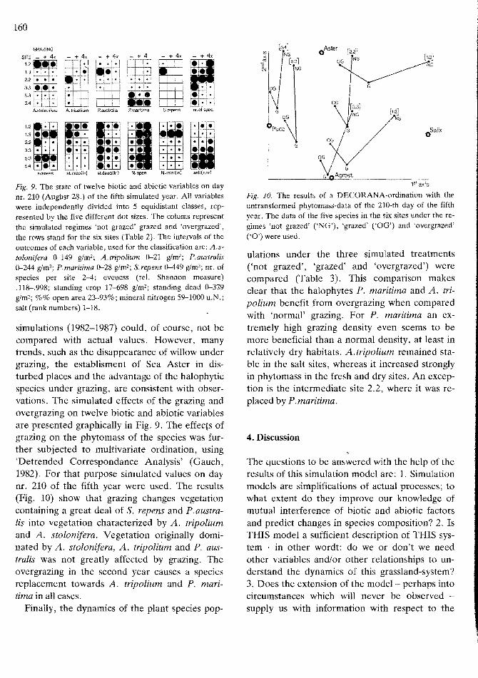
Fig. 9. The state of twelve biotic and abiotic variables on day nr. 210 (Augilst 28.) of the fifth simulated year. All variables were independently divided into 5 equidistant classes, rep­resented by the five different dot sizes. The colums represent the simulated regimes 'not grazed' grazed and 'overgrazed', the rows stand for the six sites (Table 2). The intervals of the outcomes of each variable, used for the classification are: A.s­tolonilera 0-149 g/m2; A.tripolium 0-21 glm2; P.australis 0-244 g/m2; P.maritima 0-28 g!m2; S.repens 0-449 glm2; nr. of species per site 2-4; eveness (reL Shannon measure) .118-.998; standing crop 17-698 glm2; standing dead 0-37.9 g/m2; %% open area 23-93%; mineral nitrogen 59-1000 u.N.; salt (rank numbers) 1-18.

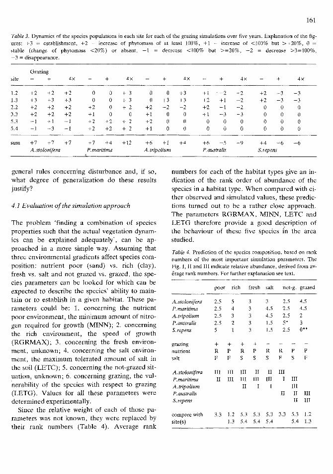
simulations (1982-1987) could, of course, not be compared with actual values. However, many trends, such as the disappearance of willow under grazing, the establisment of Sea Aster in dis­turbed places and the advantage of the halophytic species under grazing, are consistent with obser­vations. The simulated effects of the grazing and overgrazing on twelve biotic and abiotic variables are presented graphically in Fig. 9. The effects of grazing on the phytomass of the species was fur­ther subjected to multivariate ordination, using 'Detrended Correspondance Analysis' (Gauch, 1982). For that purpose simulated values on day nr. 210 of the fifth year were used. The results (Fig. 10) show that grazing changes vegetation containing a great deal of S. repens and P. austra­lis into vegetation characterized by A. tripolium and A. stolonifera. Vegetation originally domi­nated by A. stolonifera, A. tripolium and P. aus­tralis was not greatly affected by grazing. The overgrazing in the second year causes a species replacement towards A. tripolium and P. mari­tima in all cases.

Finally, the dynamics of the plant species pop-

Fig. 10. The results of a DECORANA-ordination with the untransformed phytomass-data of the 210-th day of the fifth year. The data of the five species in the six sites under the re­gimes 'not grazed' CNG'), 'grazed' ('OG') and 'overgrazed' ('0') were used.

ulations under the three simulated treatments (,not grazed', 'grazed' and 'overgrazed') were compared (Table 3). This comparison makes clear that the halophytes P. maritima and A. tri­polium benefit from overgrazing when compared with 'normal' grazing. For P. maritima an ex­tremely high grazing density even seems to be more beneficial than a normal density, at least in relatively dry habitats. A.tripolium remained sta­ble in the salt sites, whereas it increased strongly in phytomass in the fresh and dry sites. An excep­tion is the intermediate site 2.2, where it was re­placed by P.maritima.

4, Discussion

The questions to be answered with the help of the results of this simulation model are: 1. Simulation models are simplifications of actual processes; to what extent do they improve our knowledge of mutual interference of biotic and abiotic factors and predict changes in species composition? 2. Is THIS model a sufficient description of THIS sys­tern· in other wordt: do we or don't we need other variables and/or other relationships to un­derstand the dynamics of this grassland-system? 3. Does the extension of the model- perhaps into circumstances which will never be observed ­supply us with information with respect to the

161

Table 3. Dynamics of the species populations in each site for each of the grazing simulations over five years. Explanation of the fig­ures: +3 establishment, +2 = increase of phytomass of at least 100%, +1 = increase of <100% but >=20%, 0 stable (change of phytomass <20%) or absent, -1 = decrease <100% but >=20%, -2 = decrease >3=100%, - 3 = disappearance.

Grazing site + 4x + 4x + 4x + 4x + 4x

1.2 +2 +2 +2 0 0 + 3 0 0 +3 +1 . -2 -2 +2 -3 -3 1.3 +3 +3 +3 0 0 + 3 0 +3 +3 +2 +1 -2 +2 -3 -3 2.2 +2 +2 +2 +2 0 + 2 +2 -2 -2 +2 -1 -2 0 0 0 3.3 +2 +2 +2 +1 0 0 +1 0 0 +1 -3 -3 0 0 0 5.3 -1 +1 -1 +2 +2 + 2 +2 0 0 0 0 0 0 0 0 5.4 -1 -3 -1 +2 +2 + 2 +1 0 0 0 0 0 0 0 0

sum +7 +7 +7 +7 +4 +12 +6 +1 +4 +6 -5 -9 +4 ~6 -6 A.stolonifera P.maritima A.tripalium P. australis S.repens

general rules concerning disturbance and, if so, what degree of generalization do these results justify?

4.1 Evaluation of the simulation approach

The problem 'finding a combination of species properties such that the actual vegetation dynam­ics can be explained adequately', can be ap­proached in a more simple way. Assuming that three environmental gradients affect species com­position: nutrient poor (sand) vs. rich (clay), fresh vs. salt and not grazed vs. grazed, the spe­cies parameters can be looked for which can be expected to describe the species' ability to main­tain or to establish in a given habitat. These pa­rameters could be: 1. concerning the nutrient poor environment, the minimum amount of nitro­gen required for growth (MINN); 2. concerning the rich environment, the speed of growth (RGRMAX); 3. concerning the fresh environ­ment, unknown; 4. concerning the salt environ­ment, the maximum tolerated amount of salt in the soil (LETC); 5. concerning the not-grazed sit­uation, unknown; 6. concerning grazing, the vul­nerability of the species with respect to grazing (LETG). Values for all these parameters were determined experimentally.

Since the relative weight of each of those pa­rameters was not known, they were replaced by their rank numbers (Table 4). Average rank

numbers for each of the habitat types give an in­dication of the rank order of abundance of the species in a habitat type. When compared with ei­ther observed and simulated values, these predic­tions turned out to be a rather close approach. The parameters RGRMAX, MINN, LETC and LETG therefore provide a good description of the behaviour of these five species tn the area studied.

Tabllt 4. Prediction of the species composition, based on rank numbers of the most important simulation parameters. The Fig.!, II and III indicate relative abundance, derived from av­erage rank numbers. For further explanation see text.

poor rich fresh salt not-g. grazed

A.stolonifera P.maritima A.tripalium P. australis 5.repens

2.5 2.5 2.5 2.5 5

5 4 3 2

3 3 3 3 3

3 4.5 4.5 1.5 1.5

2.5 2.5 2.5 5* 2.5

4.5 4.5 2 3 0*'

grazing nutrient salt

+ R F

+ P F

+ R S

+ P S

R S

R F

P S

P F

A.stalanifera P.maritima A.tripalium P. australis S.repens

III II

III III

III III II

II III

II III

III

II

III III II II

III III

compare with site(s)

3.3 1.2 1.3

5.3 5.4

5.3 5.4

5.3 5.4

3.3 5.3 5.4

1.2 1.3

162

The simulation does, however, provide more information thqn such an analysis and the simple relationships given above. Effects, such as distur­bance and the influence of varying weather condi­tions can only be investigated with the help of a simulation programme, where the relationships between the variables are expressed as math­ematical equations. Changes in the model can be evaluated whether or not they provide an im­provement by means of comparison with actual values. However, this type of simulation ap­proach is yet only possible for simple species-poor comm unities.

4.2 The sufficiency of the model

The model described here has developed by grad­ual extension. It is still being extended, for exam­ple the species Calamagrostis epigeios and Alope­curus geniculatus have recently been included. The edaphic factors were selected gradually. Cli­matic variables have been introduced after simu­lations showed them to be necessary.

The addition of externally developed sub-mod­els and the development of sub-models as sepa­rate projects constitutes a danger in that they can introduce a large number of variables and param­eters. The programme would then acquire a pre­tention which it cannot prove. In this context: the nomenclature and the origin of the parameters concerning the nitrogen-cycle could suggest that this model simulates a nitrogen cycle, but ,this is not so: in fact this has been emphasised by the use of an exclusive relative dimension (u.N). The aim of the procedures used in this model is to describe the relevant variations in soil fertility, taking into account factors such as changes of the nitrogen contents of newly formed phytomass, and compe­tition for nutrient as a resource. Having studied the results of greenhouse experiments and field observations, we concluded that those phenom­ena were indispensable for the understanding of vegetation dynamics.

Sensitivity analysis of the parameters used showed the simulation model to be not too sensi­tive with respect to variation in any parameter. An independent variation of each of the parame­

ters, with plus and minus ten percent, resulted in a maximum deviation of two percent. Initial va­lues do have a clear effect. In the simulations demonstrated observed field values were used as starting values. The influence of (properties of) plant species that were not included in the model could not be determined.

Considering that the within-season dynamics did not depart systematically from the values that were measured in 1982 and 1983 (Table 2, Fig. 6), the conclusion can be drawn that the variables chosen and the values given to them, closely ap­proach reality in this arithmetical arrangement.

If the model is used for further prediction, the system must be observed for a longer period of time, and more experimental disturbance must be imposed: more theory-building may also be needed. Even then it is not sure that simulation will be more successful than an inductive predic­tion. In order to formulate hypotheses, and to de­sign experimentation, simulation is a time-saving alternative to experiments, and as such an attrac­tive approach.

4.3 The use ofsimulating disturbance

In the introduction of this paper we tried to ex­plain that building an explanatory model of dis­turbance in plant communities is a task which cannot, in general, be fulfilled. Through the oc­currence of unexpected events the reliability of a prediction with such a model would be low. To obtain insight in the course of processes to be ex­pected after disturbaqce, the plant species, in­volved in the simulation should represent suffi­cient variation of life and growth forms. With re­spect to strategies the dispersion mechanisms are of particular importance.

The effect of every major disturbance is that it causes an increase in bare ground. In the area studied this means that through stronger evapora­tion at the soil surface this is to cause an increase of the concentration of sodium-chloride in the up­per soil layer, though this may be reversed by 'wet' disturbance. The saltier environment is ben­eficious to halophytic plant species as has been observed in salt marsh systems (Hansen, 1982),

163

although Bakker (1985) found that grazing bene­fitted halophytic plant species, where no increase of the salt concentration in the top soil could be measured.

Simulation cannot replace numerical analysis (direct or indirect) of the biocoenoses in ques­tion. Explanatory simulation and description by means of numerical techniques rather supplement each other in the process of getting to understand vegetation dynamics (Weinstein & Shugart, 1983).

The results of this simulation confirm theories about the recovery of biocoenoses after distur­bance with some time delay (Reiners, 1983). The speed with which this recovery takes place in the simulation may not entirely reproduce reality.

Application of the model to disturbances has led to a better insight in its limitations, so that a number of improvements could be carried out. We conclude that causal/logical models of sys­tems-dynamics are adequate tools, helping us to improve our understanding of processes leading to structural changes in vegetation. The main va­lue of a model is probably the experience gained during its construction. A model which is not yet finished, or perhaps never will be finished, might therefore be among the most valuable.

Acknowledgements

The authors wish to thank all those who placed the results of their field and experimental studies at our disposal (Nico Beemster, Mieleke van Oeursen, Cor Oijkstra, Jan van Esch, Bart Friso, Eric Quene, Willy Schulten, Maarten Smit, Willy Strik, Hanneke Terpstra, everyone we forget to mention here, and Dr. Wouter Joenje and Ir. Hans Drost, who coordinated the field work). We are also grateful to those who helped to improve the manuscript by making remarks on language, style and contents, especially Dr. Roy Snaydon. Finally our thanks are due to E. Leeuwinga and O. Visser for drawing the graphs.

References

Bakker, J.P. (1985). The impact of grazing on plant commu­nities, plant populations and soil conditions on salt marshes. Vegetatio 62: 391-398.

Boersma, S.K.T. & Hoenderkamp, T. (1985). Simulatie, een moderne methode van onderzoek. Academic Service, The Hague. 315 pp..

Davidson, J.M., Graetz, D.A., Suresh, P.m Rao, C. & Magdi Selim, H. (1978). Simulation of nitrogen movement, trans­formation and uptake in plant root zones. Ecological Re­search Series 600/3-78-D29. Environmental Protection Agency, Athens, 105 pp.

Doyle, T.W. (1981), A simulation model of forest succession in the Puerto Rican tropical montane fores~. In: D.C. West, H.H. Shugart & D. Botkin (Eds.) Forest succession: pat­terns and applications. Springer, Berlin, Heidelberg, New York.

Ellenberg, H. (1954). Ueber einige Fortschritte der kausalen Vegetationskunde. Vegetatio 5/6: 199--211.

Fresco, L.F.M. (1982). An analysis of species response curves and of competition from field data: some results from heath vegetation. Vegetatio 48: 175-185.

Gauch, H.G.Jr. (1982). Multivariate analysis in community ecology. Cambridge University Press, Cambridge. 298 pp.

Godron, M. & Forman, R.T.T. (1983). Landscape modifica­tion and changing ecological characteristics. :(.11: H. Mooney & M. Godron (Eds.) Disturbance and ecosystems, pp 12-28. Springer, Berlin. Heidelberg, New York.

Goodall, D.W. (1969). Simulating the grazing situation. In: F. Heinmets (Ed.): Concepts and models of biomathematical simulation techniques and methods 1: 211-236. Marcel Dekker Inc., New York.

Graybeal, W. & Pooch, U.W. (1980). Simulation: principles and methods. Cambridge University Press, Cambridge.

Gremmen, N.J.M., Reijnen, M.l.S.M., Wiertz, l. & van Wir­dum, G. (1984). Modelling for the effects of groundwater withdrawal on the species composition of the vegetation in the Pleistocene areas of The Netherlands. In: Annual Re­port 1984 of the State Institute for Nature Management: 89--111.

Grime, J.P. (1979). Plant Strategies and Vegetation Proc­esses. Wiley, London. 222 pp.

Grubb, P.J. (1979). The maintenance of species-richness in plant communities: the importance of the regeneration niche. Biological Review 52: 107-145.

Hansen. D. (1982). Entwicklung und Beeinflussung der Net­toprimaerproduktion auf Vorlandflaechen und im Vogels­chutzgebiet Hauke-Haien-Koog. Schriftenreihe lnst. Was­serw. und Landschaftsoekologie Christian-Albr.-Universi­taet Kiel I: 1-273.

Jaquard, P. & Heim. G. (1983). Demographic strategies and originating environment. In: H. Mooney & Godron, M. (Eds.) Disturbance and ecosystems. pp 226-239. Springer. Berlin. Heidelberg. New York.

164

Joenje, W. (1978). Plant colonization and succession on em­banked sandflats. Thesis, Groningen. 160 pp.

Joenje, W. (1919). Plant succession and nature conservation of newly embanked flats in the Lauwerszeepolder. In: R.L. Jefferies & A.J. Davy (Eds.) Ecological processes in coastal environments, pp 617-634. Blackwell, Oxford.

Joenje, W. (1982). Nature in new Wadden-polders; conserva­tion by exploitation. In: Polders of the world. Vol. 2. pp 68-82. Pudoc, Wageningen.

Joenje, W. (1985). The significance of waterfowl grazing in the primary vegetation succession on embanked sandflats. Vegetatio 62: 399-406.

Kemmers, R.H. & Jansen, P.e. (1985). Stikstofmineralisatie in onbemest half-natuurlijke graslanden. Rapport 14, Insti­tuut voor Cultuurtechniek en Waterhuishouding, Wage­ningen. 15 pp.

Miller, P.C., Miller, P.M., Blake-Jacobson, M., Stuart Chapin III, F., Everett, K.R., Hilbert, D.W., Kummerow, J., Linkins, A.E., Marion, G.M., Oechel, W.e., Roberts, S.W. & Stuart, L. (1984). Plant-soil processes in Eriopho­rum vagina tum tussock tundra in Alaska: a systems model­ing approach. Ecological Monographs 54: 361-405.

Olson, J.S. (1963). Energy storage and the balance of produc­ers and decomposers in ecological systems. Ecology 44: 322-331.-

Peet, R.K. & Christensen, N.L. (1980). Succession: a popula­tion process. Vegetatio 43: 131-140.

Penning de Vries, F.W.T. (1984). Practical uses of dynamic and explanatory models for simulating crop growth. Wissenschaftliche Zeitschrift der Humboldt-Universitat zu Berlin, Math.-Nat,. 33: 343-345.

Reiners, W.A. (1983). Disturbance and basic properties of ecosystem energetics. In: H. Mooney & M. Godron (Eds). Disturbance and ecosystems, pp 83-98. Springer, Berlin, Heidelberg, New York.

Reitsma, J .H. (1981). De vegetatie in het Lauwersmeerge­bied in 1980. Internal report State Authority of the IJssel­lake Polders, Lelystad.

Runge, M. (1983). Physiology and ecology of nitrogen nutri­tion. In: O.L. Lange, P.S. Nobel, C.B. Osmond & H. Zieg­len (Eds.): Encyclopedia of plant physiology. New series. Vol. 12C: 163-200. Springer, New York, Berlin, Heidel­berg.

Weinstein, D.A. & Shugart, H.H. (1983). Ecological model­ing of landscape dynamics. In: H. Mooney & M. Godron (Eds.): Disturbance and ecosystems, pp 29-45. Springer, Berlin, Heidelberg, New York.

West, D.e., McLaughlin, S.B., Shugart, H.H. (1980). Simu­lated forest response to chronic air pollution stress. J. Envi­ron. Qual. 9: 43-49.

Wit, e.T. de & Goudriaan, J. (1978). Simulation of ecological processes. Pudoc, Wageningen. 167 pp.

Appendix. Information concerning the most important functions and parameters in 'EGRAS'.

Parameters explanation Value

Agr. Aster Phrgm. Pucc. Salix

RGRMAX max. reI. growth g/g/day .31 .20 .13 .21 .08 SCMAX max. carr. cap. g/m2 884 884 2000 884 2000 INTIJ coeft. of compo 0-1 all values 0, except Phrgm. and Salix, excluding (1) all species. MINN min. req. N-tot for growth

dimensionality of N: text 300 300 300 300 150 LETN lethal N-tot in soil all values VERY large. LETC lethal NaCl in top soil 97.5 162.5 19.8' 162.5 13.5 GROPT optimal grazing press. 0-1 all values 0 GRLE lethal grazing press. 0-1 1.00 1.00 .27 1.00 .05 TEMIN min. air temp. for growth e. 2 2 2 2 2 TEOPT opt. air temp. for growth e. 20 20 20 20 20 TEMAX max. air temp. for growth e. 30 30 30 30 30 UMIN min. light for growth J/cm2 100 100 100 100 100 UMAX max. light for growth J/cm2 2500 2500 2500 2500 2500 WAMIN min. water level cm -20 -20 -50 -20 -50 WAMAX max. water level-'cm +30 +10 +30 +10 ?

1. Procedures concerning growth and death All factors except RGRMAX: 0 < = factor <=1;PLGR(i) = RGRMAX x For explanation of the factors: see text. (l-SCU/SCMAX) x C x ND x NT

x ST x G x T x L x W

165

f Agr. Aster Phrgm, Puce, Salix

2. Procedures concerning grazing

The total consumable biomass in the area SCTOT. The ungrazed residual (varying per species) SCRES. The speed of consumption increases linearly with (SCTOT-SCRES), if (SCTOT-SCRES) is less than a constant SCSAT (Noy-Meir 1978). The angle of increase depends of the time of the year. If (SCTOT-SCRES) > = SCSATthen GRSP (speed of grazing in g/day) equals GRSPMAX (a constant).

For calculation of the preference-class: see text.

Parameter explanation Value

The amount of living and dead biomass, removed from the site by trampling: For each species: SCLITR = (ARTR X SCLI)/AREA, where ARTR = AREA X C3 X 32/400 and SCDETR (ARTR X SCDE)/AREA. The coefficient C3 is a function of soil moisture and the growth form of the species. The figure '32' is a consequence of an assumption that each cow-step affects 1 dm2 of the surface.

The loss of biomass by grazing (not-consumed, not-trampled) has been estimated at 1%.

All the nitrogen in the removed biomass returns to the system.

seRES residual s.cr. after grazing g dr. m .1m2 25 50 200 25 "250

PRSP relative graz. pref. ,17 .26 ,28 .26 .03

C3 a constant, depend. of growth form (s. above) ,015 .050 .024 ,015 ,050

3. Procedures concerning abiotic factors

Parameter explanation Value

Agr. Aster Phrgm. Puce. Salix

PI min. N-intake u.N.lg .0254 .0339 .0014 .0536 .0141

P2 N-intake li.N./g per In u.N. available N .0028 .0028 .0099 .0085 .0000

---..---.--------------------------~----

Salt as a function of vegetation coverage: SAMAX = ~O.021 x SUMAREA + 2.329; SAMAX is an absolute value (kg NaCl).