Embed Size (px)
Citation preview

‘Ecological Prices’ in Economic and Ecological Systems - Concepts, Problems and Solution Methods
REEDS SymposiumThe Biosphere Cycles in their Territorial ContextsUniversité de Versailles Saint-Quentin-en-YvellinesRambouilletFrance
Professor Murray Patterson School of People, Environment and PlanningMassey UniversityNew Zealand

Part 1: Contrast Concepts of ‘Ecological Prices
Part 2: Calculation of Ecological Prices, in Simple System
Part 3: Calculation of Ecological Prices, in Complicated System

Part 1: Contrast Concepts of ‘Ecological Prices’ and ‘Neoclassical Valuation of Ecosystem Services’
Part 2: Calculation of Ecological Prices, in Simple System
Part 3: Calculation of Ecological Prices, in Complicated Systems
Part 4: Problems in Calculating Ecological Prices (particularly in Complicated Systems)
Part 5: Solution Methods
Powerpoint and references will be available to you
Part 1: Concept of Ecological Prices


$$$
$$
$$$
$$
$
$$$
$$$
$$
$$$
$$
$
$$$

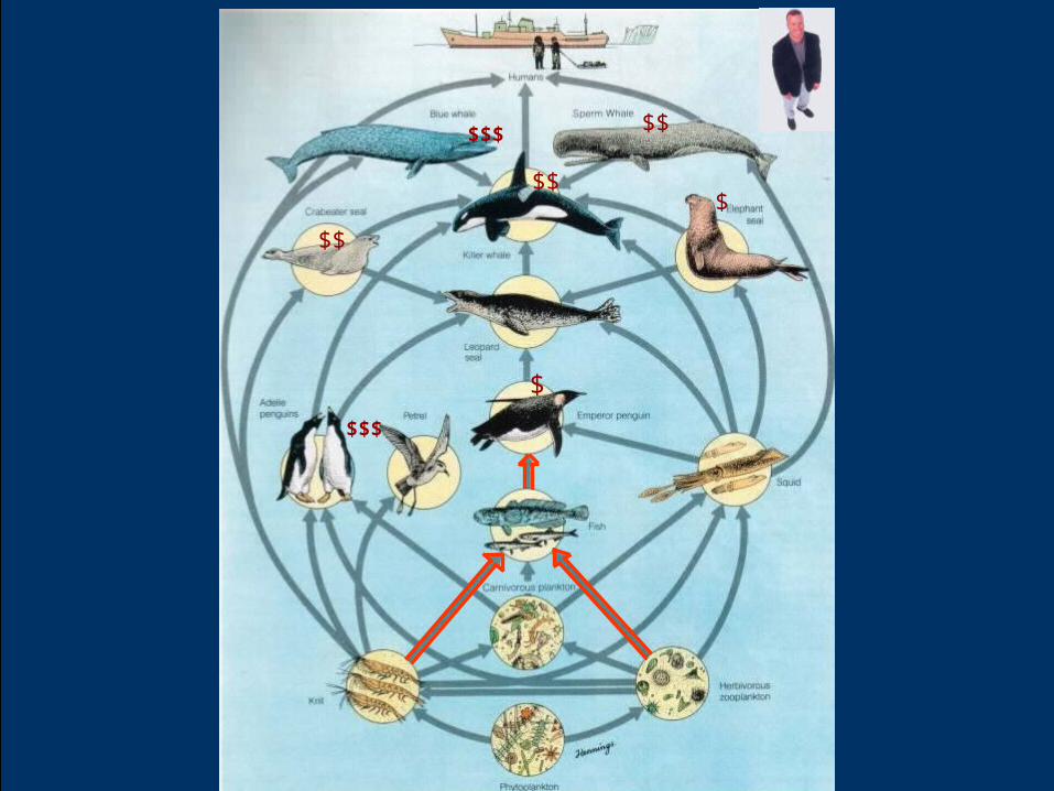
Schlei Fjord Ecosystem

Backward Linkages = embodied inputs

Backward Linkages = embodied inputs
Forward Linkages = embodied outputs

Backward Linkages = embodied inputs
Forward Linkages = embodied outputs

Solar Energy
Photosynthesis BiomassElectricity Generatio
nElectricity
3,000,000 PJ 3,000 PJ 3,000 PJ 1,000 PJ
Ecological Prices (solar equivalents)
Solar Energy : 1 PJ solar equivalents/ 1PJ solar (by definition) Biomass Energy: 1000 PJ solar equivalents/ 1 PJ biomassElectricity Energy: 3000 PJ solar equivalents/ 1 PJ electricity
Ecological Prices (electricity equivalents)
Solar Energy: 0.0003 electricity equivalents/ 1 PJ solarBiomass Energy: 0.33 electricity equivalents/ 1 PJ biomassElectricity : 1.00 electricity equivalents/ 1 PJ electricity (by definition)
More numerical example of ecological prices
Solar Energy
Photosynthesis BiomassElectricity Generatio
nElectricity
3,000,000 PJ 3,000 PJ 3,000 PJ 1,000 PJ
Uranium Ore
Mining andEnrichment
Refined Uranium
Electricity Generation
20,000 kg 4,000 kg 2,000 PJ
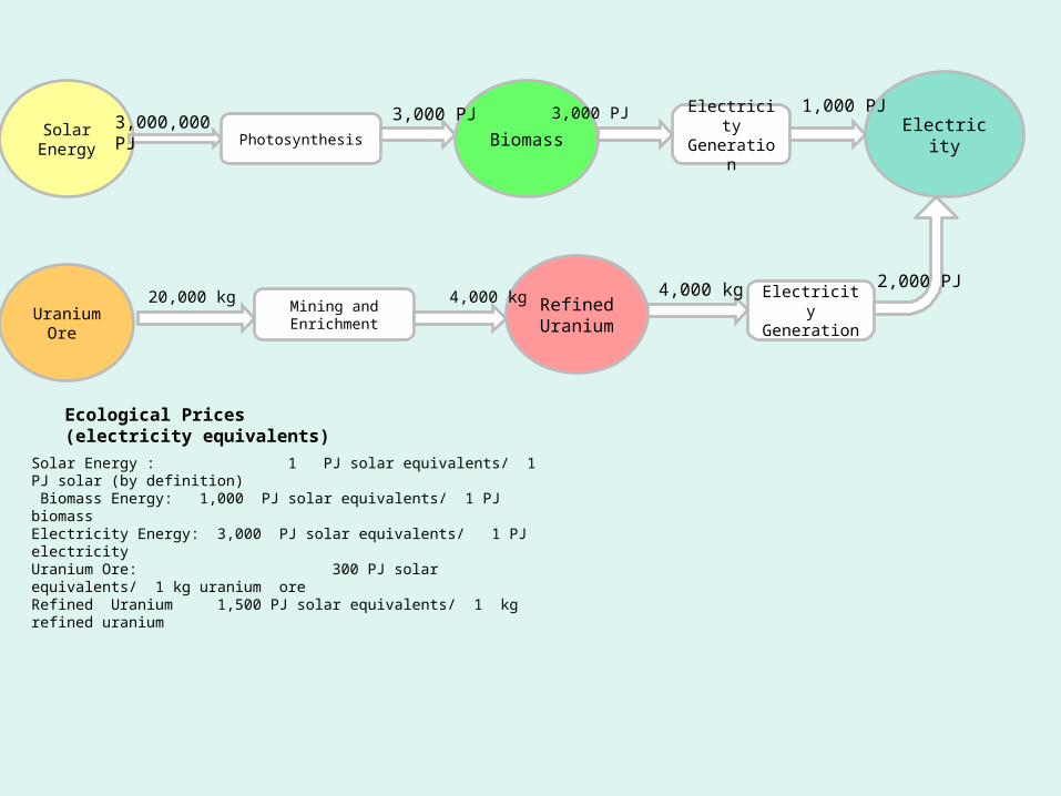
Ecological Prices (electricity equivalents)
Solar Energy : 1 PJ solar equivalents/ 1 PJ solar (by definition) Biomass Energy: 1,000 PJ solar equivalents/ 1 PJ biomassElectricity Energy: 3,000 PJ solar equivalents/ 1 PJ electricityUranium Ore: 300 PJ solar equivalents/ 1 kg uranium oreRefined Uranium 1,500 PJ solar equivalents/ 1 kg refined uranium
4,000 kg

Solar Energy
Photosynthesis BiomassElectricity Generatio
nElectricity
3,000,000 PJ 3,000 PJ 3,000 PJ 1,000 PJ
Uranium Ore
Mining andEnrichment
Refined Uranium
Electricity Generation
20,000 kg 4,000 kg 2,000 PJ
Ecological Prices (electricity equivalents)
Solar Energy : 1 PJ solar equivalents/ 1 PJ solar (by definition) Biomass Energy: 1,000 PJ solar equivalents/ 1 PJ biomassElectricity Energy: 3,000 PJ solar equivalents/ 1 PJ electricityUranium Ore: 300 PJ solar equivalents/ 1 kg uranium oreRefined Uranium 1,500 PJ solar equivalents/ 1 kg refined uranium
4,000 kg

Solar Energy
PJ
Photosynthesis
Biomass
PJ Electricity Generatio
n
Electricity
PJ
3,000,000 PJ 3,000 PJ 3,000 PJ 1,000 PJ
Uranium Ore
kg
Mining andEnrichment
Refined Uranium
kg
Electricity Generation
20,000 kg 4,000 kg 2,000 PJ
Ecological Prices (electricity equivalents)
Solar Energy : 1 PJ solar equivalents/ 1 PJ solar (by definition) Biomass Energy: 1,000 PJ solar equivalents/ 1 PJ biomassElectricity Energy: 3,000 PJ solar equivalents/ 1 PJ electricityUranium Ore: 300 PJ solar equivalents/ 1 kg uranium oreRefined Uranium 1,500 PJ solar equivalents/ 1 kg refined uranium
4,000 kg
Means that ‘1 kg uranium ore’ Is 300 times more productive than‘1 PJ of solar energy’

Solar Energy
PJ
Photosynthesis
Biomass
PJ Electricity Generatio
n
Electricity
PJ
3,000,000 PJ 3,000 PJ 3,000 PJ 1,000 PJ
Uranium Ore
kg
Mining andEnrichment
Refined Uranium
kg
Electricity Generation
20,000 kg 4,000 kg 2,000 PJ4,000 kg
Complications in the real world: more the one system output – above example, only one output = electricity many more processes processes can have multiple outputs (joint production) processes can have multiple inputs most importantly, there are ‘complicated webs’ with: feedbacks, sometimes circular flows and interactions between processes – above example has only
two straight chains

Key Features of Ecological Pricing
• Base data = energy and mass flows, economic and/or ecological systems
From this base data, ecological prices are ‘inferred’ or ‘implied’
• Ecological Prices, measure biophysical interdependencies (donor, receiver, both) in the system - eg, 1000 J solar energy 10 J Biomass
• Ecological prices are measured in ‘physical units’ –eg, -eg, : 10 GJ of Solar Energy per 1 kg of Phytoplankton-eg, : 10 Euros per 1 kg of Phytoplankton (analogous to conventional
price)

Historical Context to Ecological Pricing
1970
Ecology
Economics‘Cost of Production’ Methods
Economics ‘Subjective Preference’
Methods
Ecological Pricing ?
1983EMERGY
H T Odum
2010s
1991Contributory Value
QualityEquivalentMethodology
Patterson
1981Biosphere Input-OutputModel
Costanza et al.
1980s
Perrings, O’Connor,England, Judson
1960
Production of Commodities by Means of Commodities
Sraffa
1946
General Equilibrium Model
von Neumann
Ricardo
early 1880s
1930s- 1940s
Input-Output Analysis
Leontief
Neoclassical Economics
2013Dominant Paradigm
1997
Costanza et al.
Value of Global Ecosystem Services
1890sSupply and Demand Curves
Marshall
Extending Sraffato the Environment
1942
Energy flows in food chainsLindeman
Ulanowicz

Part 2: Calculation of Ecological Prices,
In simple systems

Simplified Example
Solar Energy Photosynthesis Phyto-
plankton Consumption Zoo-plankton
Decomposition Detritus
100 GJ 50 kg 46 kg 36 kg
26 kg4 kg
30 kg
Step 1 - Diagramming
= quantity
= process

Simplified Example
Solar Energy Photosynthesis Phyto-
plankton Consumption Zoo-plankton
Decomposition Detritus
100 GJ 50 kg 46 kg 36 kg
26 kg4 kg
30 kg
Step 1 - Diagramming
= quantity
= process
Which quantity’s ‘price’ is based on: donor value only? receiver value only?

Step 2 : Convert Diagram to Matrix Format
Solar Energy Phytoplankton Zooplankton Detritus100 GJ kg kg kg
Photosynthesis -100 50Consumption -46 36Decomposition -4 -26 30
Negative number = process input
Positive number = process output

Step 2 : Convert DiagramMatrix Format
Solar Energy Phytoplankton Zooplankton Detritus100 GJ kg kg kg
Photosynthesis -100 50Consumption -46 36Decomposition -4 -26 30
Negative number = process input
Positive number = process output
Which quantity’s price is based on: donor value only? receiver value only?
Step 2 : Convert Diagram toMatrix Format

Step 2 : Convert Diagram to Matrix Format
Step 3: Convert to a System of Simultaneous Equations
100p1 = 50p2
46p2 + 6p4 = 36p3
4p2 + 26p3 = 30p4
Inputs on ‘left side’ of the equation
Outputs of the ‘right side’ of the equation
Solar Energy Phytoplankton Zooplankton Detritus100 GJ kg kg kg
Photosynthesis -100 50Consumption -46 36Decomposition -4 -26 30

Step 3: Convert to a System of Simultaneous Equations
100p1 = 50p2
46p2 + 6p4 = 36p3
4p2 + 26p3 = 30p4
Inputs on ‘left side’ of the equation
Outputs of the ‘right side’ of the equation
Step 4: Solve the Equations, to obtain the ecological prices
3 equations, 4 unknownsTherefore, underdetermined by 1 degree of freedom
p1 = 1 (by
definition)p2 = 2.00
p3 = 3.04
p4 = 2.90
Solar energy in the numeraire

Step 3: Convert to a System of Simultaneous Equations
100p1 = 50p2
46p2 + 6p4 = 36p3
4p2 + 26p3 = 30p4
Inputs on ‘left side’ of the equation
Outputs of the ‘right side’ of the equation
Step 4: Solve the Equations, to obtain the ecological prices
3 equations, 4 unknownsTherefore, underdetermined by 1 degree of freedom
Therefore, need to set one quantity to unity (one):That quantity becomes the ‘numeraire’; The system becomes determined (3 equations, 3 unknowns)
p1 = 1 (by
definition)p2 = 2.00
p3 = 3.04
p4 = 2.90
Solar energy in the numeraire p1 = 0.50
p2 = 1.00 (by
defintion)p3 = 1.52
p4 = 1.45
Phytoplankton is the numeraire

p1 = 1 (by
definition)p2 = 2.00
p3 = 3.04
p4 = 2.90
Solar energy in the numeraire
p1 = 0.50
p2 = 1.00 (by
definition)p3 = 1.52
p4 = 1.45
Phytoplankton is the numeraire
The relativities between the prices stay the same (Irrespective the choice of selected numeraire) –ie, they are ‘relative prices’
2 2
Part 3: Problems of Ecological Prices,
In complicated systems

Quick overview of the types on complicated systems we are analysing

Schlei Fjord Ecosystem

Units =PJ of energy
New Zealand EnergySystem

Units = Pg of carbon
Biosphere

Units = Pg of nitrogen
Biosphere

Units = Pg of sulphur
Biosphere

Units = Pg of H20
• Units =
Biosphere

Global Economy
Units = Pg

Units = EJ of energy
World

Summary: Ecological and Economic Systems Analysed
YearMatrix Dimensions Linkages Joint Products Negative Prices Matrix Singularity
New Zealand Energy System 1980 35 x 12 65 NoneNew Zealand Energy System 1987 45 x 20 225 NoneSmall National Energy System 9 x 5 11 NoneWorld Energy System 1994 23 x 9 53 NoneSchlei Fjord Germany 1983 13 X 14 32 NoneSilver Springs Ecosystem 1955 10 x 9 13 NoneOyster Ecosystem 1973 8 x 7 34 NoneBiosphere 1980 9 x 10 Some yes yesBiosphere 1994 23 x 23 93 Some yes yesBiosphere 1994 120 x 80 612 Numerous yes yes
Always, described in terms of ‘energy and/or mass flows’
Therefore, must have conservation of energy and mass - ie: for each process:
∑energy outputs + energy ‘waste’ =∑energy inputs ∑mass outputs + mass ‘waste’ =∑mass inputs

Now for the ‘problems’ with ‘complicated systems’ ……..

Problem #1 =Non-Square Matrix
• Problem = unequal number of processes and unknown prices
• Really a ‘degrees of freedom’ problem: Over-determined (processes > quantities). Determined (processes = quantities) Under-determined by 1 df (processes + 1= quantities Under-determined (processes< quantities)
• Solution Methods: Over-determined: least squares fitting Determined: eigen-solution Under-determined by 1 df: matrix inversion Under-determined: optimisation

In
Solar Energy (Joules)
Bio
mass
(kg
s)
Out
Problem #2 = Inconsistent Equations
20 p1 = 1 p2
30 p1 = 2 p2
40 p1 = 1.1 p2
20 p1 + e130 p1
40 p1
Can’t Solve ‘Solve’ by including residuals
Tree Species 1
Tree Species 2
Tree Species 3
+ e2
+ e3
= 1 p2
= 1.1p2
= 2 p2
e2e3
e1
p1 = ecological price
= average conversion ratio of solar energy to biomass

Inconsistent Equations = Different Process Efficiencies
p1 = 1 20 p1 + e1
30 p1
40 p1
+ e2
+ e3
= 1 p2
= 1.1p2
= 2 p2 p2 = 22
(C) Substitute prices into (1), (2), (3)
20 x 1 + 2 = 1 x 22
30 x 1 + 14 = 2 x 22
40 x 1 + 15.6 = 1.1 x 22
(D) Divide outputs by inputs = Process efficiency ξ1 = 1.10
ξ2 = 1.47
ξ3 = 0.61
e1 = 2
e2 = 14
e3 = -15.8
(A) Base Equations (B) Equation solutions
Price x Quantity = Value
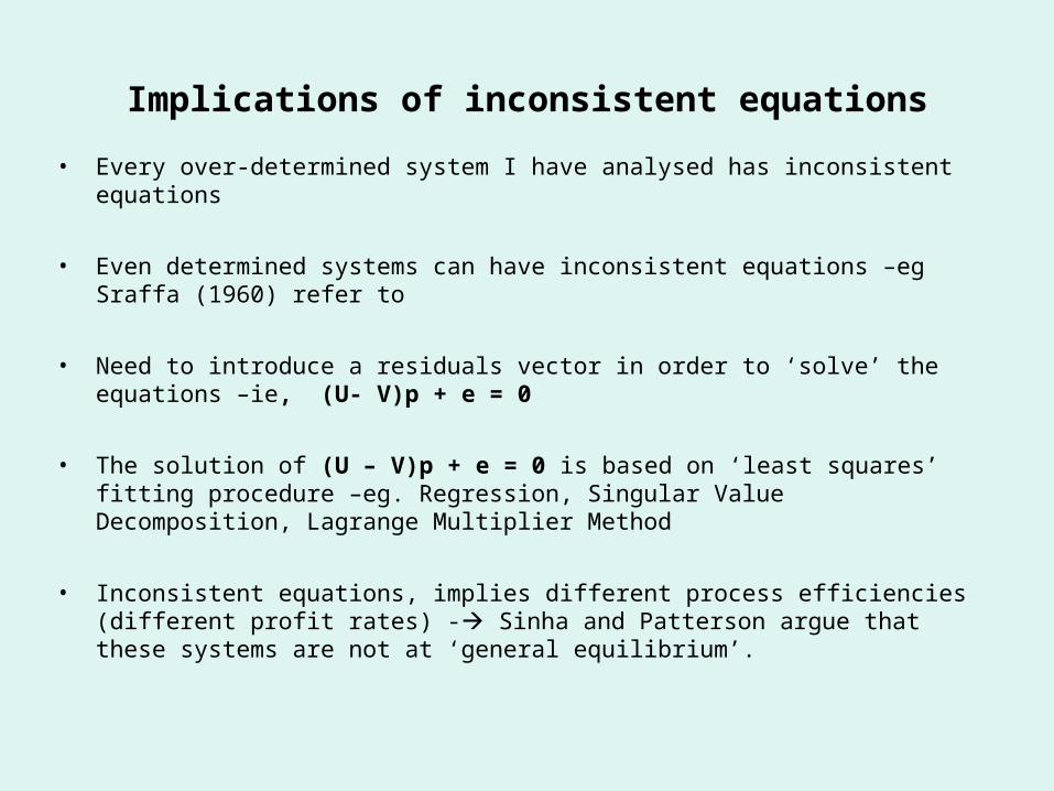
Implications of inconsistent equations
• Every over-determined system I have analysed has inconsistent equations
• Even determined systems can have inconsistent equations –eg Sraffa (1960) refer to
• Need to introduce a residuals vector in order to ‘solve’ the equations –ie, (U- V)p + e = 0
• The solution of (U – V)p + e = 0 is based on ‘least squares’ fitting procedure –eg. Regression, Singular Value Decomposition, Lagrange Multiplier Method
• Inconsistent equations, implies different process efficiencies (different profit rates) - Sinha and Patterson argue that these systems are not at ‘general equilibrium’.

Problem #3 = Joint Production
• Joint Production is an inherent property of ‘economic’ and ‘ecological’ systems:
- eg: solar energy + C02 +H20 Carbohydrates+ O2
• Only a problem with the standard Leontief input-output formulation which assumes ‘one output per process (sector)’:
(I-At)p = q
• Stone and others from the 1960’s started to use ‘make’ (outputs) and ‘use’ (inputs) matrices – the ‘make’ matrix can have multiple outputs per sector
(U - V)p = q
• Joint production is a ‘problem’ in-so-far as it often leads to negative prices in the solution vector.
Outputs Inputs Price
numeraire quantity
Inputs (use) matrix Outputs (make) matrix

Problem #4: Negative Prices
• Many large joint products negative prices are inevitable - eg, biosphere models
• Two possible approaches for dealing with this problem: Costanza (1984) sets non-negativity constraint (p > 0) Patterson (2014) reflexive approach. Costanza’s approach generates lots of zero transformities,
Patterson’s reflexive approach doesn’t

Problem # 5: Matrix Singularity
•linear dependence between rows in U – V matrix matrix singularity matrix cannot be inverted equations cannot be solved.
• Example: Water cycle in Costanza and Neil (1981)
•Can be overcome by Patterson’s (2011) ‘singular value decompostion’ method

Part 4: Solution Methods for Calculating Ecological Prices

Sraffa (1960) + Others
• Strictly speaking, he didn’t calculate ‘ecological prices’.
• However: There are similarities between Sraffa’s method, and ecological pricing Ecological economists have extended Sraffa’s method to include
interactions with the biophysical environment –eg,Perrings, O’Connor, Mayumi, Judson
• Passenti (1979) provided Eigensolution of Sraffa’s model, so that prices p and profit rate r could be calculated from U – V
MAIN PROBLEMS:•Assumes square matrix (processes= quantity)•Assumes same profit rate for all processes• No constructive way in dealing with ‘matrix singularity’ and ‘negative prices’

Regression Method: Patterson (1983)
( U – V)p + e = g
Where: U – V = Outputs – Inputs matrix, measured energy units g = numeraire vector p = price vector, to be solved for e = vector of residuals, to be solved for
Solution Method: Step 1: Move one column in U - V to the ‘right hand side’ and change sign.
The selected column is the numeraire quantity. Step 2: Repeat Step 1, for all of the columns in U - V Step 3: Select numeraire with highest R2
MAIN PROBLEMS:• ‘Prices’ numerically vary (slightly), depending on which numeraire is used• Highest R2 of n models, may not be the ‘best’ of all possible models

Matrix Inversion Costanza, Hannon & Others (mid1980’s)
MAIN PROBLEMS:• Only applicable to square matrices (m = n)• (Falsely) assumes that solar energy is the only valid numeraire•All processes assumed to have same efficiency (profit rate) of unity• Encountered negative prices•Encountered matrix singularity
p = g (U - V)-1
Where:U = outputs matrix (m x n), mass and/or energy units V = inputs matrix (m x n), mass and /or energy unitsg = numeraire vector (1 x n) of solar energy p = price vector (1 x m) , to be solved for
[

Linear Optimisation:Costanza and Neill (1984)
[Maximise (Dual): q = pz (total value of net output of the system) (8)Subject to: p(U - V) = g (value constraints)
p≥ 0 (ie, non-negative prices)Where:U = outputs matrix (m x n), mass and/or energy units V = inputs matrix (m x n), mass and /or energy unitsg = numeraire vector (1 x n) of solar energyp = price vector (1 x m) , to be solved forz = vector (m x 1) of net quantity outputs the system (energy and/or mass units)
q = scalar (1 x 1) total value of net output from the system (price x quantity = value)
MAIN PROBLEMS:•In the optimal solution: Non-negativity constraint led to many zero prices for some quantities Zero activity for ‘inefficient’ processes
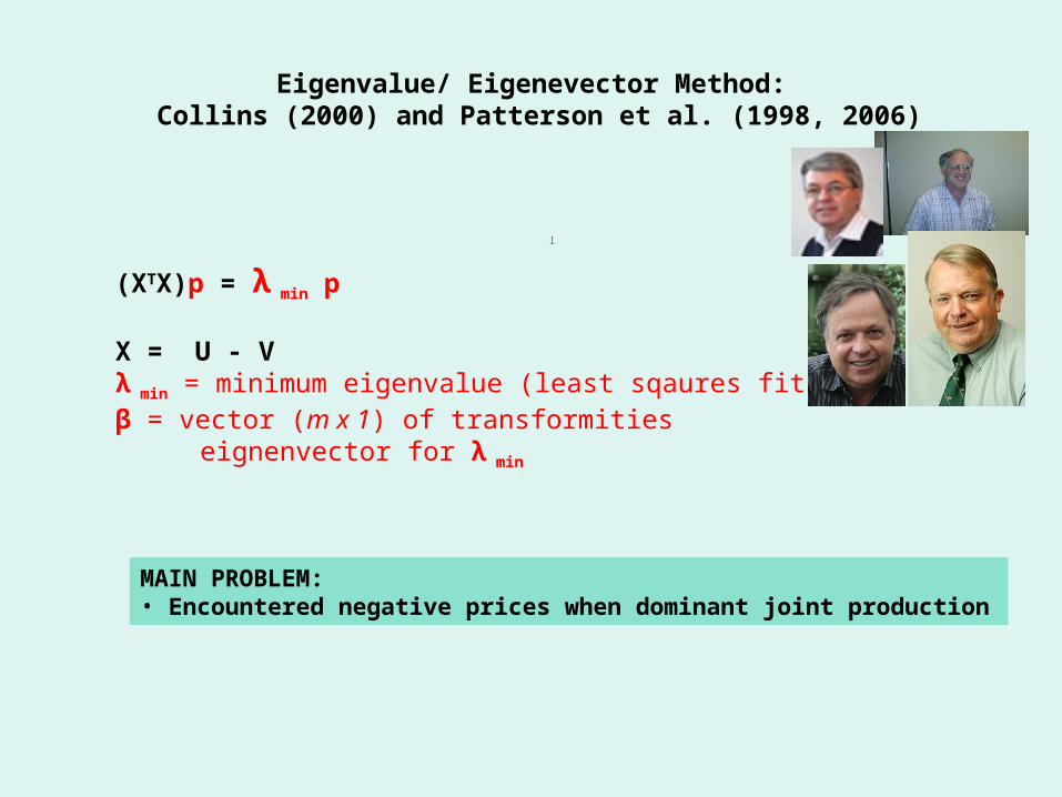
Eigenvalue/ Eigenevector Method: Collins (2000) and Patterson et al. (1998, 2006)
(XTX)p = λ min p
X = U - Vλ min = minimum eigenvalue (least sqaures fit)β = vector (m x 1) of transformities
eignenvector for λ min
[
MAIN PROBLEM:• Encountered negative prices when dominant joint production

Singular Value Decomposition: Patterson (2012)
[The Singular Value Decomposition consists of the factorisation:
X = UDLT
Where:U = orthogonal matrix (n x n) consisting of ‘left hand singular’ vectorsLT = orthogonal matrix (m x m) consisting of ‘right hand singular’ vectorsD =non-negative diagonal matrix (n x m) of singular values, in descending order
The least squares solution for the prices p is given by the column of LT (which corresponds to the smallest diagonal entity of D)
NOTE:• Exactly the same numerical results as ‘Eigenvalue/ Eigenvector’ Method Mathematicians would probably consider SVD to be a more ‘elegant solution’ •Singular Value Decomposition can be applied to any real matrix (non- square, singular etc) ;unlike eigen-solution (a la Sraffa)
MAIN PROBLEM:• Encountered negative prices when dominant joint production

Reflexive Method: Patterson (2014)Outputs – Inputs Matrix
(U-V)Process x Quantity
Usually Rectangular
STEP 2: Partition processes into sub-
processes based on prices – ‘looking’ Forwards (for inputs) & Backwards (for
outputs)
STEP 3: Add up all sub-processes with the same
quantity
STEP 1:Initial guess/estimate
Forward Linkages Matrix H
Quantity x QuantityUsually Under-determined
Backward Linkages Matrix G
Quantity x QuantityUsually Under-determined
STEP 4:H + G = W
‘Double Entry’Book-keeping
Kernel Matrix WQuantity x QuantityAlways Determined
Always sum of columns = zero
Price Vector p
STEP 5:Solve equations Wp = 0
SVD most elegant solution method
Emulates (I- A) matrix which
ensures no
negative prices, by Perron -
Frobenius Theorem
ADVANTAGE:• Solves negative price problem.
MAIN PROBLEM:• Difficult to explain complicated algorithm

Which Solution Method is Best?
SraffaEigen-
solution
Regression Method
Matrix Inversion;
input-output analysis
LinearOptimisation
Eigenvalue-Eigenvector / Singular Value Decomposition
Reflexive Method
Non-square matrices Problem Okay Problem Marginal Okay Okay
Joint Production (co-products
Okay Okay Okay, but not with Traditional
Leontief
Okay Okay Okay
Negative Prices Problem Problem Problem Marginal Problem Okay
Matrix Singularity Problem Problem Problem Okay Okay Okay
Unequal Process Efficiencies/ Profit Rates
Problem Okay Problem Marginal Okay Okay
Specification of Numeraire
Okay Marginal Marginal Marginal Okay Okay
Mathematical Proofs/Formalism/Elegance
Okay Okay Okay Okay Okay Marginal?Problem?

Conclusions
• For simple systems all solution methods give the same answer
• For complicated systems (joint production, structural complexity, processes ≠ quantities, etc):
negative prices can result Matrix singularity can occur non-square matrices occurTherefore, more sophisticated methods are required !!!
• All ‘solution methods’ are described in published journal articles –see:
‘References’ on next page, or email: [email protected]

ReferencesCollins, D. and Odum, H.T. 2000. Calculating transformities with an eigenvector method. In: Brown, M.T. (Ed.) Energy
synthesis: Theory and applications of the energy methodology. Centre for Environmental Policy, University of Florida, Gainesville.
Costanza, R. and Neill, C., 1981. The energy embodied in products of the biosphere. In: Mitsch, W.J., Boserman, R.W. and Klopatek, J.M. (Eds.), Energy and ecological modelling. Elsevier, Amsterdam, pp. 745-755.
Costanza, R. and Neill, C. 1984. Energy intensities, interdependence and value in ecological systems: a linear programming approach. Journal of Theoretical Biology, 106, 41-57
Costanza R, d’Arge R, de Groot R, Farber S, Grasso M, Hannon B, Limburg K, Naeem S, O’Neill RV, Paruelo J, Raskin RG, Sutton P, van den Belt M 1997. The value of the world’s ecosystem service and natural capital. Nature 387, 253–260
England, R.W. 1986. Production, distribution and environmental quality: Mr Sraffa reinterpreted as an ecologist. Kylos 39: 230-244
Judson, D.H. 1989. The convergence of neo-ricardian and embodied energy theories of value and price. Ecological Economics, 1, 261-281.
Mayumi, K., 1999. Embodied energy analysis, Sraffa’s analysis, Georgescu-Roegen’s flow-fund model and viability of solar technology. In: Mayumi, K., Gowdy J.M. (Eds.), Bioeconomics and Sustainability. Edward Elgar, Cheltenham, United Kingdom, pp. 173-193.
O'Connor, M., 1993. Value system contests and the appropriation of ecological capital. The Manchester School of Economic & Social Studies, 61, 398-424
Pasinetti, L. 1977. Essays on the theory of joint production. MacMillan Press, LondonPatterson, M.G. 1983. Estimation of the quality of energy sources and uses. Energy Policy, 11:4, 346-359.Patterson, M.G. 1998. Understanding energy quality in economic and ecological Systems. In Advances in Energy
Studies: Energy Flows in Ecology and Economy. pp.257-274. Museum of Science and Scientific Information, Rome.
Patterson M.G. 1998. Commensuration and theories of value in ecological economics, Ecological Economics, 25:1, 105–123.
Patterson, M.G. 2002. Ecological production-based pricing biosphere processes. Ecological Economics, 41, 457-478.Patterson, M.G., Wake, G.C, McKibbin, R and Cole, A.O. 2006. Ecological pricing and transformity: A solution method for
systems rarely at general equilibrium. Ecological Economics, 56, 412-423. Patterson, M, G. 2012. Are all processes equally efficient from an emergy perspective?: Analysis of ecological and
economic networks using matrix algebra methods. Ecological Modelling 226, 71-91 Patterson, M.G. 2014. Evaluation of matrix algebra methods for calculating transformities from ecological and economic
network data. Ecological Modelling 271, 72-82

Perrings, C., 1986. Economy and environment: a theoretical essay on the interdependence of economic and environmental systems. Cambridge University Press, Cambridge
Sraffa, P. 1960. Production of commodities by means of commodities: prelude to a critique of economic theory. Cambridge University Press, Cambridge
Ulanowicz, R.E. 1991. ‘Contributory values of ecosystem resources’, in R. Costanza (ed.), Ecological Economics: The Science and Management of Sustainability, New York: Columbia University Press, pp. 253–268.
von Neumann, J., 1946. A model of general economic equilibrium. The Review of Economic Studies , 13, 1-9

Thank-you!
Mathematical Details in Published Papers


63
Value Related to Policy Goals
Efficiency Sustainability Distribution
Economic Welfare(Market + pseudo
market prices)
Strong SustainabilityWeak Sustainability
Equity
Ecological Productivity / Production(ecological prices)
ResilienceIntegrity
Diversity

Complications in Solving for Ecological Prices
Non-square matrices
- eg, over-determined matrices; with more equations (processes) than unknowns (prices for each quantity)
Joint production, some processes produce more than one producteg, sheep produce meat and wool
Negative prices, are sometimes obtained in solving the equations
Inconsistent Equations, meaning no direct (non-trivial)solution to X = 0
Matrix Singularity, for some matrices which means than solution methods that rely on matrix inversion, will not work