Embed Size (px)
Citation preview

Past exam questions
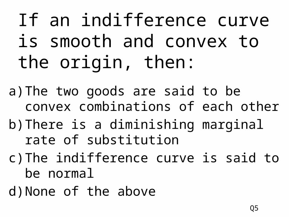
If an indifference curve is smooth and convex to the origin, then:
a) The two goods are said to be convex combinations of each other
b) There is a diminishing marginal rate of substitution
c) The indifference curve is said to be normald) None of the above
Q5
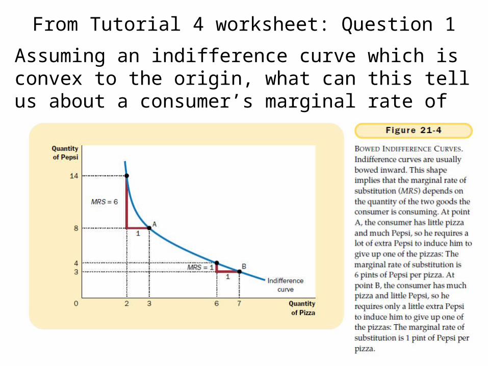
From Tutorial 4 worksheet: Question 1Assuming an indifference curve which is convex to the origin, what can this tell us about a consumer’s marginal rate of substitution between coffee and muffins?
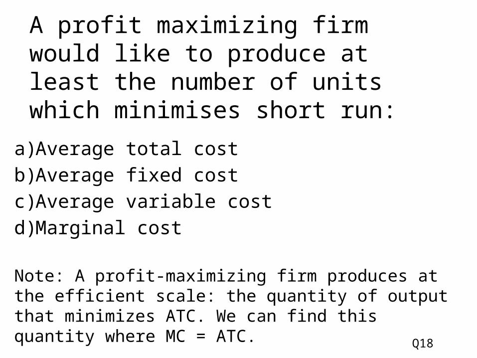
A profit maximizing firm would like to produce at least the number of units which minimises short run:
a) Average total costb) Average fixed costc) Average variable costd) Marginal cost
Note: A profit-maximizing firm produces at the efficient scale: the quantity of output that minimizes ATC. We can find this quantity where MC = ATC. Q18
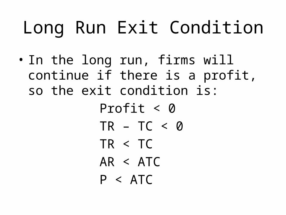
Long Run Exit Condition
• In the long run, firms will continue if there is a profit, so the exit condition is:
Profit < 0TR – TC < 0TR < TCAR < ATCP < ATC
Short Run Exit Condition
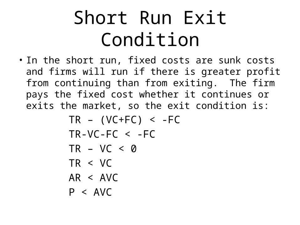
• In the short run, fixed costs are sunk costs and firms will run if there is greater profit from continuing than from exiting. The firm pays the fixed cost whether it continues or exits the market, so the exit condition is:
TR – (VC+FC) < -FCTR-VC-FC < -FCTR – VC < 0TR < VCAR < AVCP < AVC
MC=S
P, C
0 q
AVC
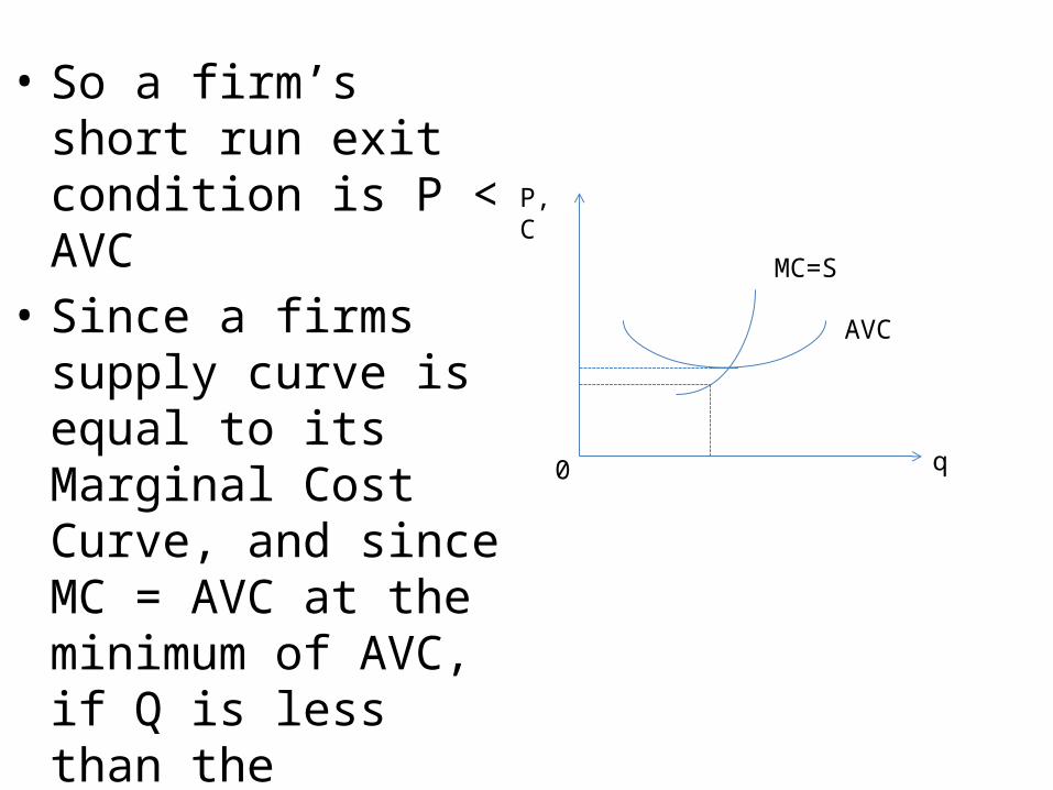
• So a firm’s short run exit condition is P < AVC
• Since a firms supply curve is equal to its Marginal Cost Curve, and since MC = AVC at the minimum of AVC, if Q is less than the quantity that minimizes AVC, P will be less than AVC for that Q.
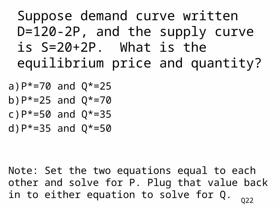
Suppose demand curve written D=120-2P, and the supply curve is S=20+2P. What is the equilibrium price and quantity?
a) P*=70 and Q*=25b) P*=25 and Q*=70c) P*=50 and Q*=35d) P*=35 and Q*=50
Note: Set the two equations equal to each other and solve for P. Plug that value back in to either equation to solve for Q. Q22
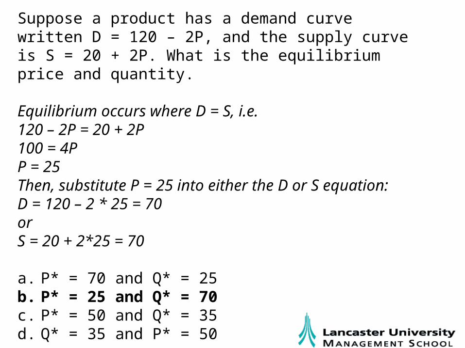
Suppose a product has a demand curve written D = 120 – 2P, and the supply curve is S = 20 + 2P. What is the equilibrium price and quantity.
Equilibrium occurs where D = S, i.e.120 – 2P = 20 + 2P100 = 4PP = 25Then, substitute P = 25 into either the D or S equation:D = 120 – 2 * 25 = 70orS = 20 + 2*25 = 70
a. P* = 70 and Q* = 25b. P* = 25 and Q* = 70c. P* = 50 and Q* = 35d. Q* = 35 and P* = 50
Suppose demand is given by D=120-2P and supply is originally S=20+2P but the government imposes a tax of 10 on this good. What happens to the equilibrium price?
a) Rises by 10b) Rises by 8c) Rises by 5d) Rises, but it’s not possible to say by how much
Q23
We have D=120-2P and S=20+2P Then a tax of 10 is imposed on this good. What happens to the equilibrium price?
There are two ways we can solve this. 1. By assuming that the tax is placed on consumers,
thus affecting the Demand curve (shifting it to the left)
2. By assuming that the tax is placed on suppliers/sellers, thus affecting the Supply curve (shifting it to the left).
I’ll work through both methods in the following slides.
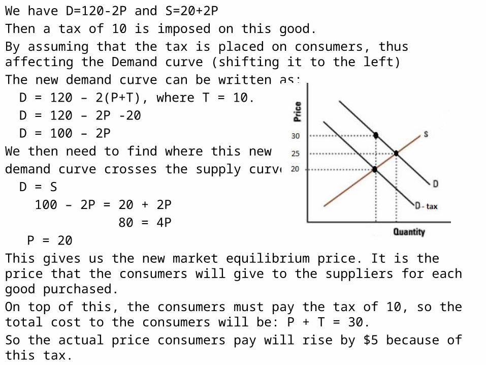
We have D=120-2P and S=20+2P Then a tax of 10 is imposed on this good. By assuming that the tax is placed on consumers, thus affecting the Demand curve (shifting it to the left)The new demand curve can be written as:
D = 120 – 2(P+T), where T = 10.D = 120 – 2P -20D = 100 – 2P
We then need to find where this new demand curve crosses the supply curve.
D = S 100 – 2P = 20 + 2P 80 = 4P P = 20
This gives us the new market equilibrium price. It is the price that the consumers will give to the suppliers for each good purchased. On top of this, the consumers must pay the tax of 10, so the total cost to the consumers will be: P + T = 30. So the actual price consumers pay will rise by $5 because of this tax.
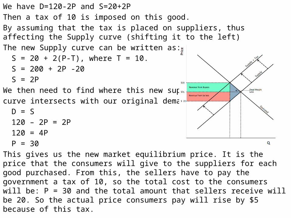
We have D=120-2P and S=20+2P Then a tax of 10 is imposed on this good. By assuming that the tax is placed on suppliers, thus affecting the Supply curve (shifting it to the left)The new Supply curve can be written as:
S = 20 + 2(P-T), where T = 10.S = 200 + 2P -20S = 2P
We then need to find where this new supply curve intersects with our original demand curve.
D = S120 – 2P = 2P120 = 4PP = 30
This gives us the new market equilibrium price. It is the price that the consumers will give to the suppliers for each good purchased. From this, the sellers have to pay the government a tax of 10, so the total cost to the consumers will be: P = 30 and the total amount that sellers receive will be 20. So the actual price consumers pay will rise by $5 because of this tax.
Suppose D=10/P, work out the price elasticity at P=10 and P = 20 and P=30.
a) Not possible to say without knowing what the corresponding level of demand is.
b) -1, -2, -3c) -3, -2, -1d) -1, -1, -1
Q25
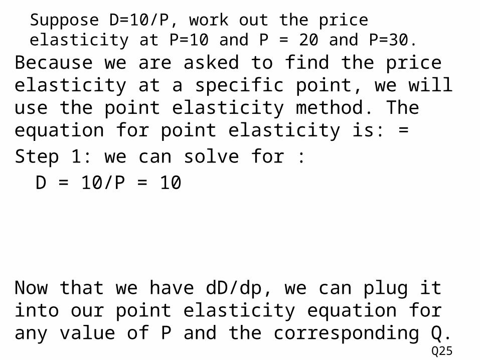
Suppose D=10/P, work out the price elasticity at P=10 and P = 20 and P=30.
Because we are asked to find the price elasticity at a specific point, we will use the point elasticity method. The equation for point elasticity is: = Step 1: we can solve for :
D = 10/P = 10
Now that we have dD/dp, we can plug it into our point elasticity equation for any value of P and the corresponding Q. Q25
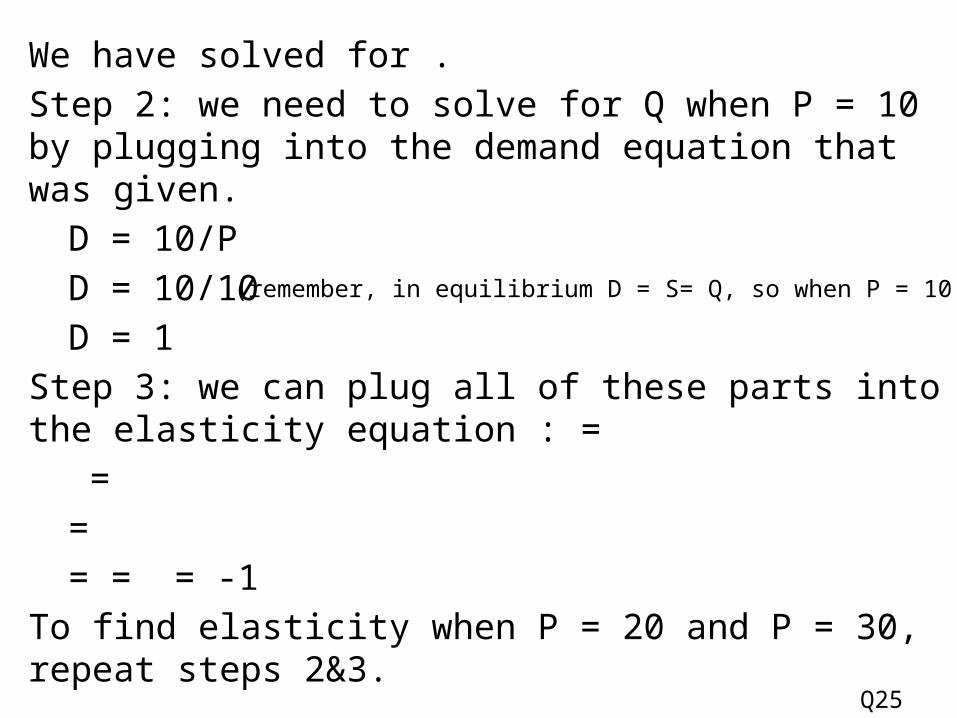
We have solved for .Step 2: we need to solve for Q when P = 10 by plugging into the demand equation that was given.
D = 10/PD = 10/10 D = 1
Step 3: we can plug all of these parts into the elasticity equation : =
=== = = -1
To find elasticity when P = 20 and P = 30, repeat steps 2&3. Q25
(remember, in equilibrium D = S= Q, so when P = 10, Q = 1))
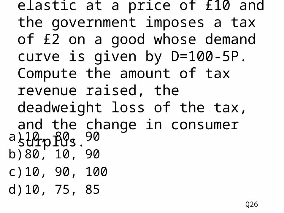
Suppose supply is perfectly elastic at a price of £10 and the government imposes a tax of £2 on a good whose demand curve is given by D=100-5P. Compute the amount of tax revenue raised, the deadweight loss of the tax, and the change in consumer surplus.
a) 10, 80, 90b) 80, 10, 90c) 10, 90, 100d) 10, 75, 85
Q26
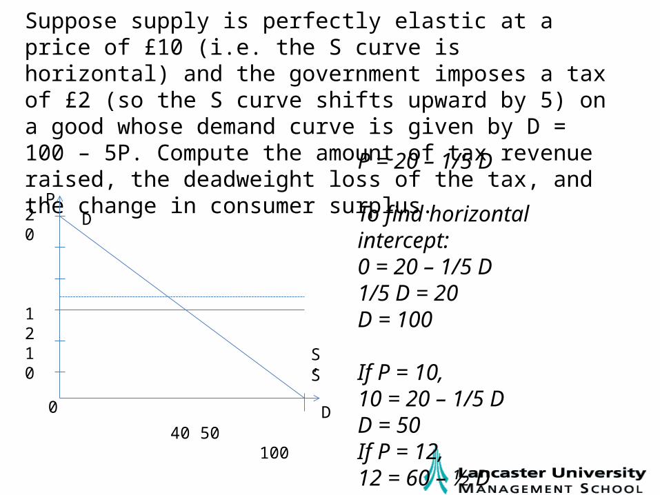
Suppose supply is perfectly elastic at a price of £10 (i.e. the S curve is horizontal) and the government imposes a tax of £2 (so the S curve shifts upward by 5) on a good whose demand curve is given by D = 100 – 5P. Compute the amount of tax revenue raised, the deadweight loss of the tax, and the change in consumer surplus.
P
0 D
20
1210
SS’
P = 20 – 1/5 D
To find horizontal intercept:0 = 20 – 1/5 D1/5 D = 20D = 100
If P = 10, 10 = 20 – 1/5 DD = 50If P = 12,12 = 60 – ½ DD = 40
D
40 50 100
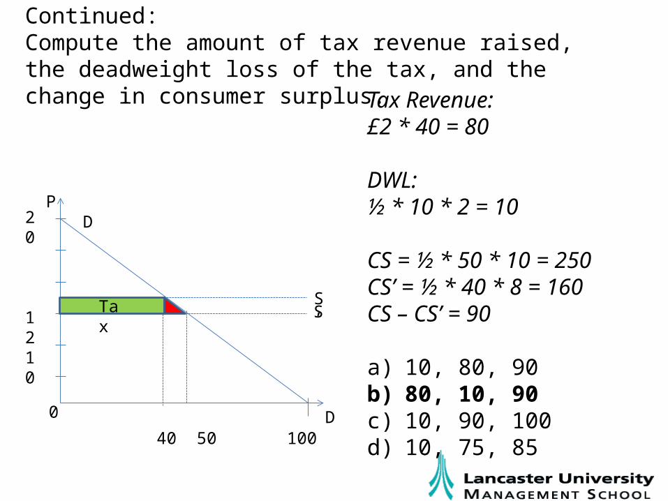
Continued:Compute the amount of tax revenue raised, the deadweight loss of the tax, and the change in consumer surplus.
P
0 D
20
1210 S
S’
D
40 50 100
Tax Revenue:£2 * 40 = 80
DWL:½ * 10 * 2 = 10
CS = ½ * 50 * 10 = 250CS’ = ½ * 40 * 8 = 160CS – CS’ = 90
a) 10, 80, 90b) 80, 10, 90c) 10, 90, 100d) 10, 75, 85
Tax
Suppose the TC curve for a firm where TC=12+4Q+Q2 and MR=8. What level of output will the firm produce in order to maximise profit (ie where MC=MR)?
a) 0b) 2c) 4d) 8
Q30
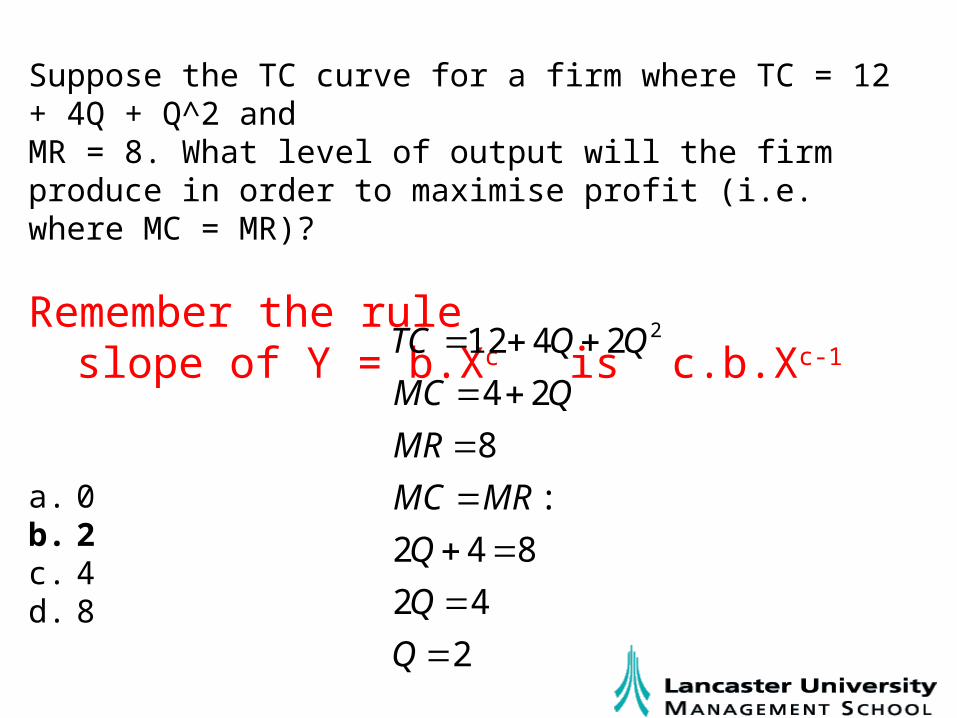
Suppose the TC curve for a firm where TC = 12 + 4Q + Q^2 and MR = 8. What level of output will the firm produce in order to maximise profit (i.e. where MC = MR)?
Remember the ruleslope of Y = b.Xc is c.b.Xc-1
a. 0b. 2c. 4d. 8
2
42
842
:
8
24
2412 2
Q
Q
Q
MRMC
MR
QMC
QQTC

Exam this Friday• 50 minutes:
– 30 questions; 20 Caroline, 10 Ian• Check your timetable for exam time and location.• Don’t forget to bring the following items:
– Library Card Number– Pencil and Eraser– Basic calculator (no programmable calculators or cell
phones will be allowed.)
Good Luck!
(For next week, check Moodle for a worksheet)

This Thursday:
Martin Ravallion Edmond D. Villani Chair in Economics, Georgetown University;
Research Associate NBER; Non-Resident Fellow CGD; Formerly Director of the World Bank’s Research Department
will deliver the
Esmée Fairbairn LectureEntitled
The Idea of Anti-Poverty Policy Lecture Theatre 1, Leadership Centre,
Management School,6.00pm Thursday 14th November 2013
Question 1If the industry under perfect competition faces a downward-sloping demand curve, why does an individual firm face a horizontal demand curve?
In a perfectly competitive market, each firm is quite small and unable to affect price on it’s own. We say that firms are price takers. This means that in a perfectly competitive market, P = MR = MC.
Question 2If supernormal profits are competed away under perfect competition, why will firms have an incentive to become more efficient?Improving efficiency can lower costs and lead to positive short run profits, based on the time it takes for competing firms to adopt the more efficient methods. In the long run, profits will go back to zero, however.
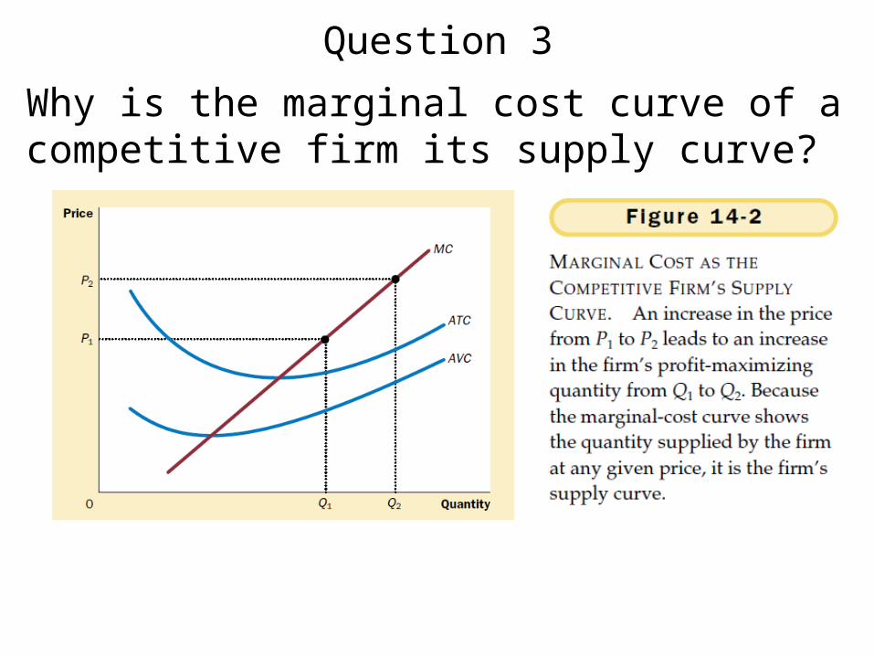
Question 3Why is the marginal cost curve of a competitive firm its supply curve?
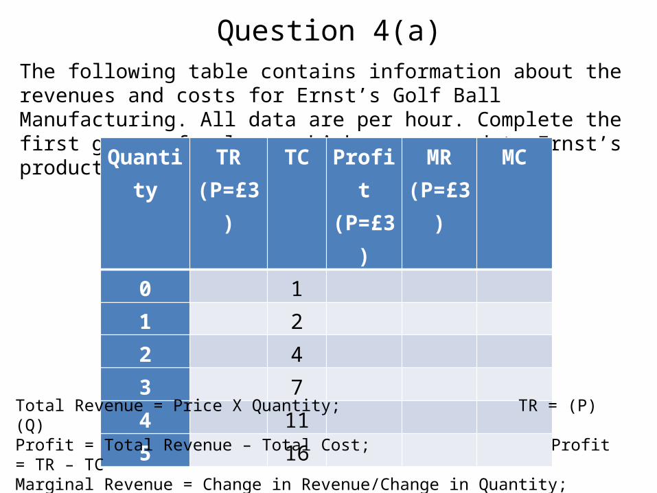
Question 4(a)The following table contains information about the revenues and costs for Ernst’s Golf Ball Manufacturing. All data are per hour. Complete the first group of columns which correspond to Ernst’s production if P = £3.
Quantity TR(P=£3)
TC Profit(P=£3)
MR(P=£3)
MC
0 1 1 2 2 4 3 7 4 11 5 16
Total Revenue = Price X Quantity; TR = (P)(Q)Profit = Total Revenue – Total Cost; Profit = TR – TCMarginal Revenue = Change in Revenue/Change in Quantity; MR = (TR2-TR1)/(Q2-Q1)Marginal Cost = Change in Cost/Change in Quantity; MC = (TC2-TC1)/(Q2-Q1)
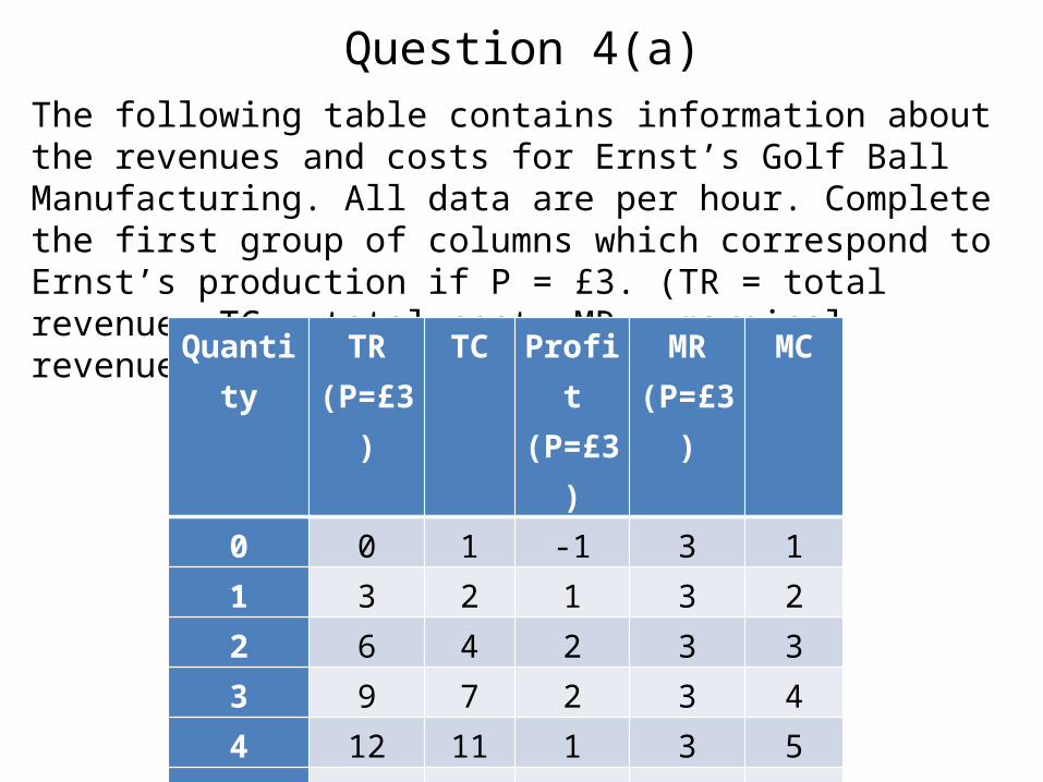
Question 4(a)The following table contains information about the revenues and costs for Ernst’s Golf Ball Manufacturing. All data are per hour. Complete the first group of columns which correspond to Ernst’s production if P = £3. (TR = total revenue, TC = total cost, MR = marginal revenue, MC = marginal cost)
Quantity TR(P=£3)
TC Profit(P=£3)
MR(P=£3)
MC
0 0 1 -1 3 1
1 3 2 1 3 2
2 6 4 2 3 3
3 9 7 2 3 4
4 12 11 1 3 5
5 15 16 -1
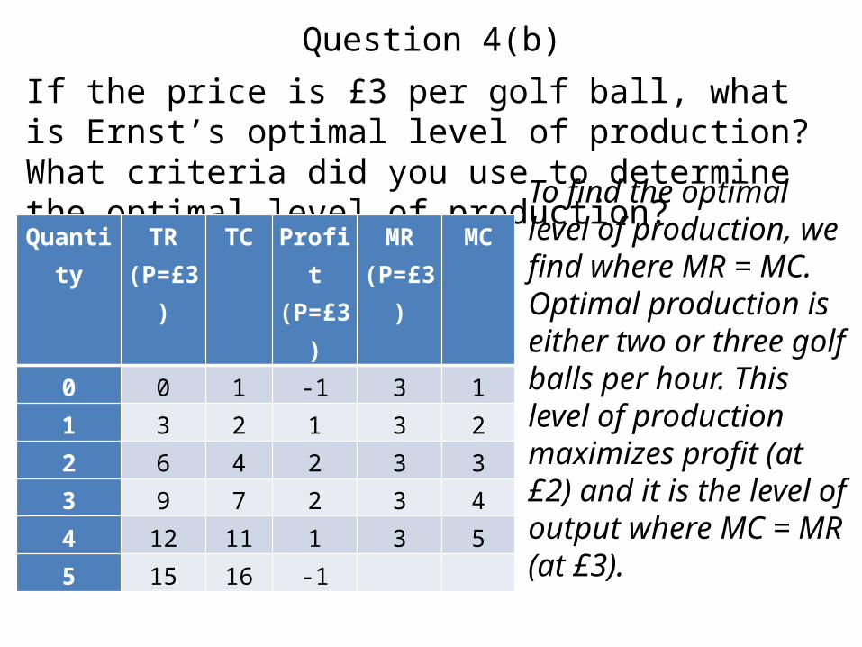
Question 4(b)If the price is £3 per golf ball, what is Ernst’s optimal level of production? What criteria did you use to determine the optimal level of production?
Quantity TR(P=£3)
TC Profit(P=£3)
MR(P=£3)
MC
0 0 1 -1 3 11 3 2 1 3 22 6 4 2 3 33 9 7 2 3 44 12 11 1 3 55 15 16 -1
To find the optimal level of production, we find where MR = MC. Optimal production is either two or three golf balls per hour. This level of production maximizes profit (at £2) and it is the level of output where MC = MR (at £3).
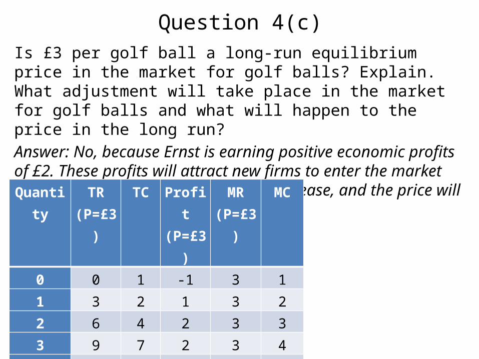
Question 4(c)Is £3 per golf ball a long-run equilibrium price in the market for golf balls? Explain. What adjustment will take place in the market for golf balls and what will happen to the price in the long run? Answer: No, because Ernst is earning positive economic profits of £2. These profits will attract new firms to enter the market for golf balls, the market supply will increase, and the price will fall until economic profits are zero. Quantity TR
(P=£3)TC Profit
(P=£3)MR
(P=£3)MC
0 0 1 -1 3 1
1 3 2 1 3 2
2 6 4 2 3 3
3 9 7 2 3 4
4 12 11 1 3 5
5 15 16 -1
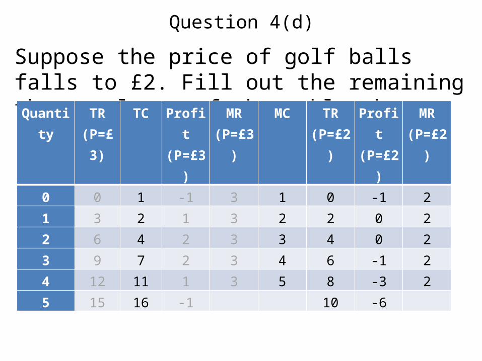
Question 4(d)Suppose the price of golf balls falls to £2. Fill out the remaining three columns of the table above.
Quantity TR(P=£3)
TC Profit(P=£3)
MR(P=£3)
MC TR(P=£2)
Profit(P=£2)
MR(P=£2)
0 0 1 -1 3 1 0 -1 21 3 2 1 3 2 2 0 22 6 4 2 3 3 4 0 23 9 7 2 3 4 6 -1 24 12 11 1 3 5 8 -3 25 15 16 -1 10 -6
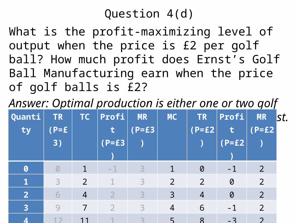
Question 4(d)What is the profit-maximizing level of output when the price is £2 per golf ball? How much profit does Ernst’s Golf Ball Manufacturing earn when the price of golf balls is £2? Answer: Optimal production is either one or two golf balls per hour. Zero economic profit is earned by Ernst.
Quantity TR(P=£3)
TC Profit(P=£3)
MR(P=£3)
MC TR(P=£2)
Profit(P=£2)
MR(P=£2)
0 0 1 -1 3 1 0 -1 21 3 2 1 3 2 2 0 22 6 4 2 3 3 4 0 23 9 7 2 3 4 6 -1 24 12 11 1 3 5 8 -3 25 15 16 -1 10 -6
Question 4(e)Is £2 per golf ball a long-run equilibrium price in the market for golf balls? Explain. Why would Ernst continue to produce at this level of profit? Answer: Yes. Economic profits are zero, therefore firms will neither enter nor exit the industry. Zero economic profits means that Ernst doesn’t earn anything beyond his opportunity costs of production but his revenues do cover the cost of his inputs and the value of his time and money.
Question 4(f)Describe the slope of the short-run supply curve for the market for golf balls. Describe the slope of the long-run supply curve in the market for golf balls.
The slope of the short-run supply curve is positive because when P = £2, quantity supplied is one or two units per firm and when P = £3, quantity supplied is two or three units per firm. In the long run, supply is horizontal (perfectly elastic) at P = £2 because any price above £2 causes firms to enter and drives the price back to £2.
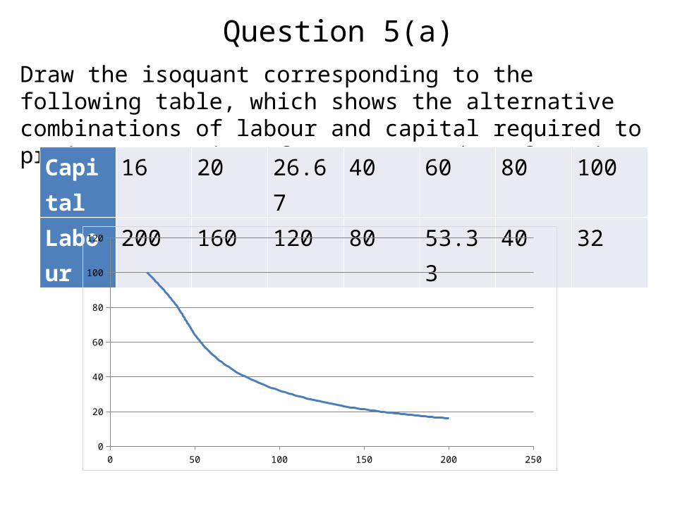
Question 5(a)Draw the isoquant corresponding to the following table, which shows the alternative combinations of labour and capital required to produce 100 units of output per day of good X.
Capital 16 20 26.67 40 60 80 100Labour 200 160 120 80 53.33 40 32
0 50 100 150 200 2500
20
40
60
80
100
120
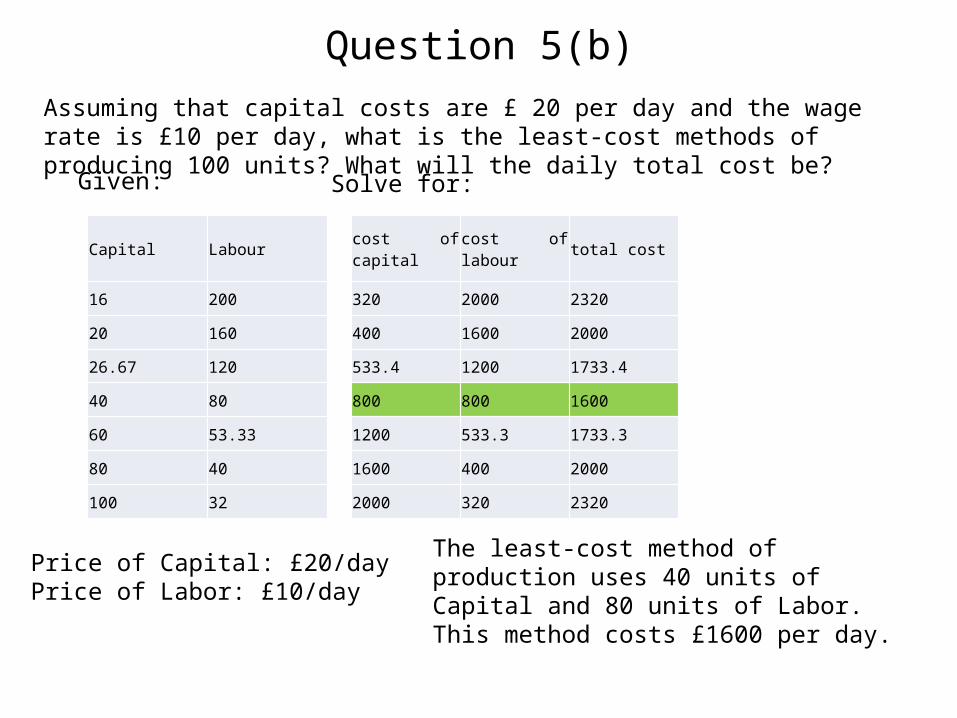
Question 5(b)
Capital Labour
16 200
20 160
26.67 120
40 80
60 53.33
80 40
100 32
cost of capital cost of labour total cost
320 2000 2320
400 1600 2000
533.4 1200 1733.4
800 800 1600
1200 533.3 1733.3
1600 400 2000
2000 320 2320
Given: Solve for:
Price of Capital: £20/dayPrice of Labor: £10/day
The least-cost method of production uses 40 units of Capital and 80 units of Labor. This method costs £1600 per day.
Assuming that capital costs are £ 20 per day and the wage rate is £10 per day, what is the least-cost methods of producing 100 units? What will the daily total cost be?
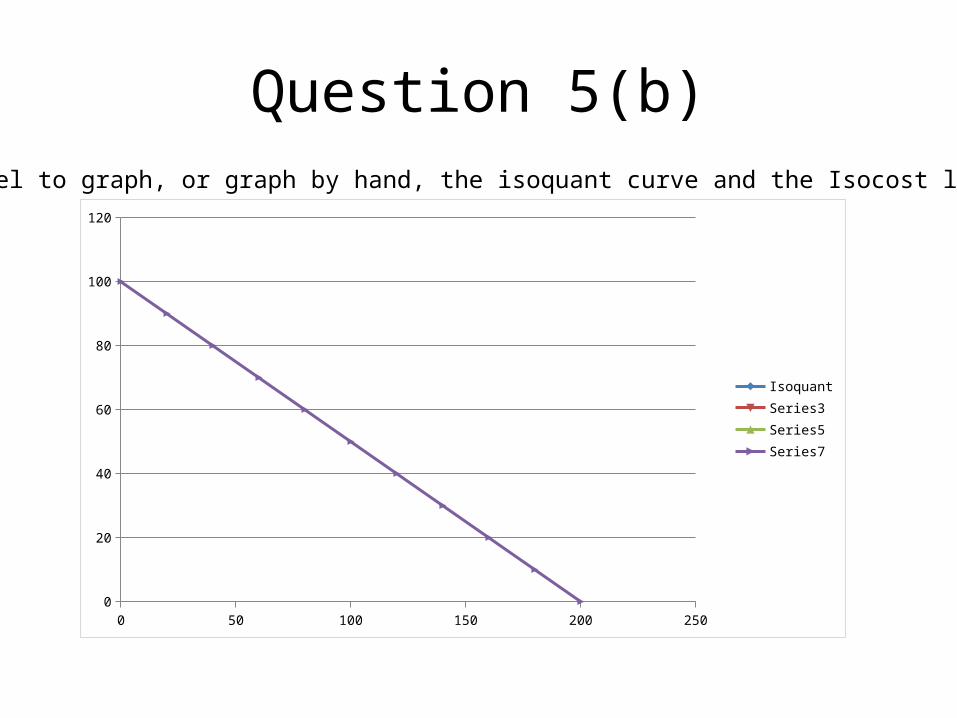
Question 5(b)
0 50 100 150 200 2500
20
40
60
80
100
120
IsoquantSeries3Series5Series7
Use Excel to graph, or graph by hand, the isoquant curve and the Isocost lines:
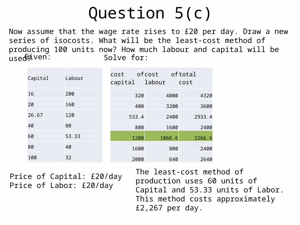
Question 5(c)
Capital Labour
16 200
20 160
26.67 120
40 80
60 53.33
80 40
100 32
cost of capital cost of labour total cost
320 4000 4320
400 3200 3600
533.4 2400 2933.4
800 1600 2400
1200 1066.6 2266.6
1600 800 2400
2000 640 2640
Given: Solve for:
Price of Capital: £20/dayPrice of Labor: £20/day
The least-cost method of production uses 60 units of Capital and 53.33 units of Labor. This method costs approximately £2,267 per day.
Now assume that the wage rate rises to £20 per day. Draw a new series of isocosts. What will be the least-cost method of producing 100 units now? How much labour and capital will be used?
Question 6In a downturn firms want to layoff some workers. This has an effect on productivity (output per employee). On the one hand, it frees up some machinery that the remaining workers can use more flexibly – you don’t have to hang around so much waiting for a machine to become free. On the other hand, workers have to do a wider ranges of tasks because there are fewer workers – so the firm loses some of the advantages of specialisation. Suppose the output of the firm, Q, depends on the number of workers, L, and the number of machines, K, in such a way that Q=LaKb Suppose a=0.4 and b=0.6.
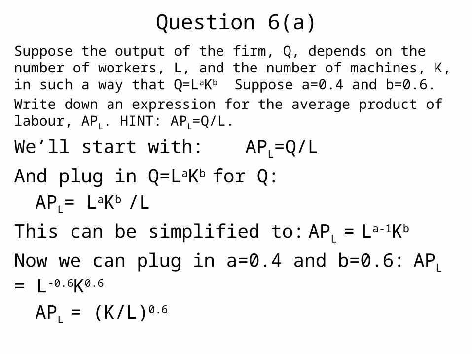
Question 6(a)Suppose the output of the firm, Q, depends on the number of workers, L, and the number of machines, K, in such a way that Q=LaKb Suppose a=0.4 and b=0.6.Write down an expression for the average product of labour, APL. HINT: APL=Q/L.
We’ll start with: APL=Q/L
And plug in Q=LaKb for Q:APL= LaKb /L
This can be simplified to: APL = La-1Kb
Now we can plug in a=0.4 and b=0.6:APL = L-0.6K0.6
APL = (K/L)0.6
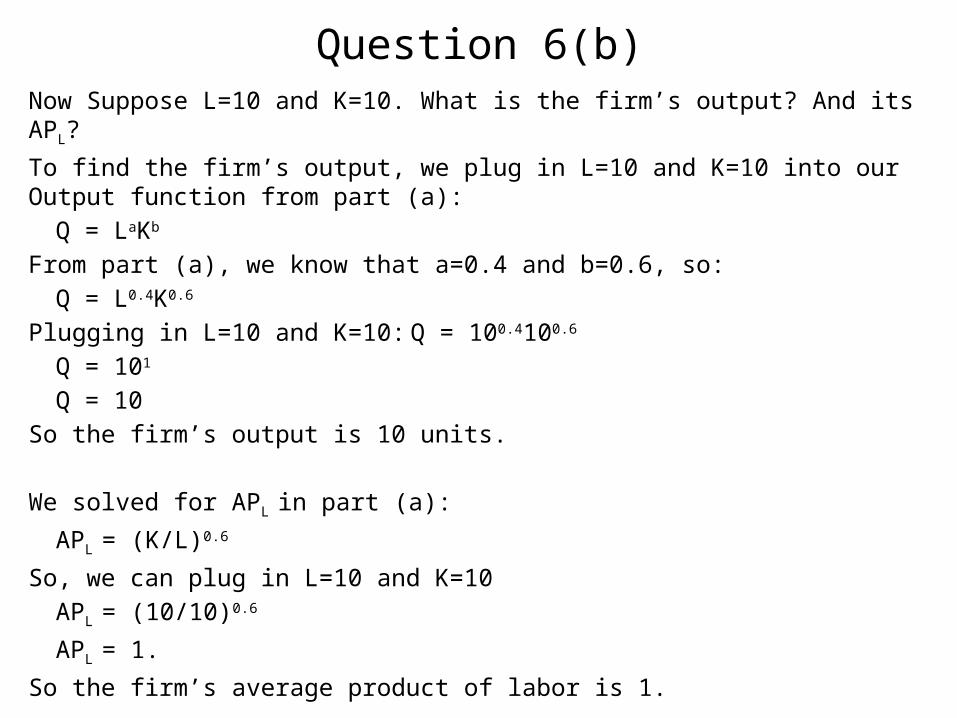
Question 6(b)Now Suppose L=10 and K=10. What is the firm’s output? And its APL?
To find the firm’s output, we plug in L=10 and K=10 into our Output function from part (a):
Q = LaKb
From part (a), we know that a=0.4 and b=0.6, so:Q = L0.4K0.6
Plugging in L=10 and K=10: Q = 100.4100.6
Q = 101 Q = 10
So the firm’s output is 10 units.
We solved for APL in part (a):
APL = (K/L)0.6
So, we can plug in L=10 and K=10APL = (10/10)0.6
APL = 1.
So the firm’s average product of labor is 1.
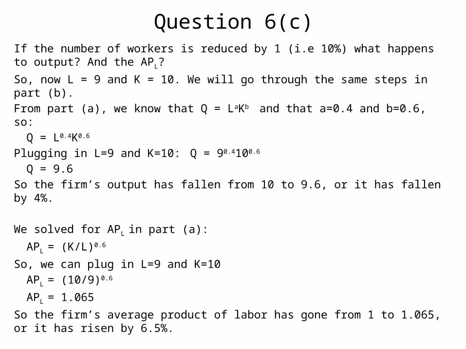
Question 6(c)If the number of workers is reduced by 1 (i.e 10%) what happens to output? And the APL?
So, now L = 9 and K = 10. We will go through the same steps in part (b).From part (a), we know that Q = LaKb and that a=0.4 and b=0.6, so:
Q = L0.4K0.6
Plugging in L=9 and K=10: Q = 90.4100.6
Q = 9.6So the firm’s output has fallen from 10 to 9.6, or it has fallen by 4%.
We solved for APL in part (a):
APL = (K/L)0.6
So, we can plug in L=9 and K=10APL = (10/9)0.6
APL = 1.065
So the firm’s average product of labor has gone from 1 to 1.065, or it has risen by 6.5%.
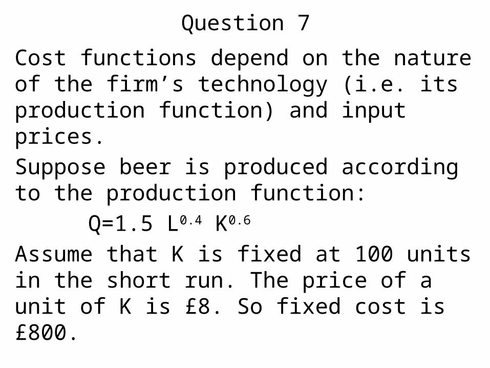
Question 7Cost functions depend on the nature of the firm’s technology (i.e. its production function) and input prices.Suppose beer is produced according to the production function:
Q=1.5 L0.4 K0.6 Assume that K is fixed at 100 units in the short run. The price of a unit of K is £8. So fixed cost is £800.
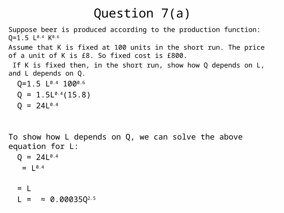
Question 7(a)Suppose beer is produced according to the production function: Q=1.5 L0.4 K0.6 Assume that K is fixed at 100 units in the short run. The price of a unit of K is £8. So fixed cost is £800. If K is fixed then, in the short run, show how Q depends on L, and L depends on Q.
Q=1.5 L0.4 1000.6 Q = 1.5L0.4(15.8)Q = 24L0.4
To show how L depends on Q, we can solve the above equation for L: Q = 24L0.4
= L0.4
= L L = ≈ 0.00035Q2.5
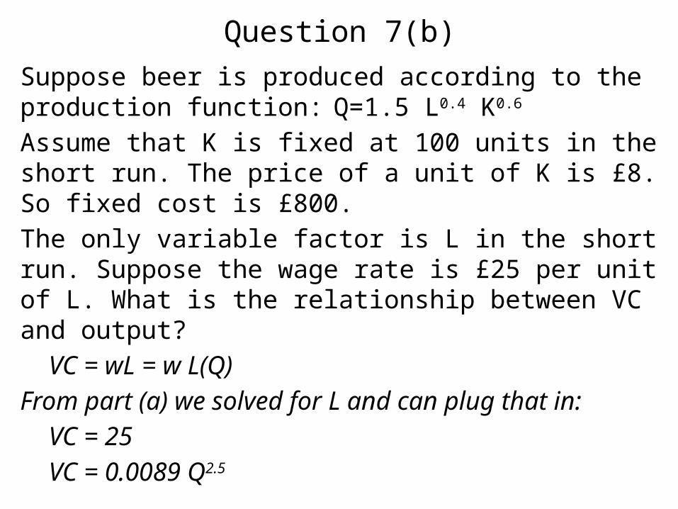
Question 7(b)Suppose beer is produced according to the production function: Q=1.5 L0.4 K0.6 Assume that K is fixed at 100 units in the short run. The price of a unit of K is £8. So fixed cost is £800. The only variable factor is L in the short run. Suppose the wage rate is £25 per unit of L. What is the relationship between VC and output?
VC = wL = w L(Q) From part (a) we solved for L and can plug that in: VC = 25
VC = 0.0089 Q2.5
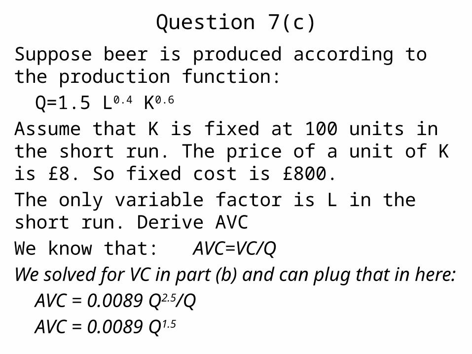
Question 7(c)Suppose beer is produced according to the production function:
Q=1.5 L0.4 K0.6 Assume that K is fixed at 100 units in the short run. The price of a unit of K is £8. So fixed cost is £800. The only variable factor is L in the short run. Derive AVCWe know that: AVC=VC/Q We solved for VC in part (b) and can plug that in here:
AVC = 0.0089 Q2.5/Q AVC = 0.0089 Q1.5
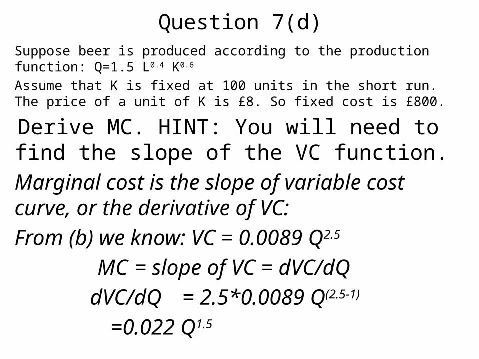
Question 7(d)Suppose beer is produced according to the production function: Q=1.5 L0.4 K0.6 Assume that K is fixed at 100 units in the short run. The price of a unit of K is £8. So fixed cost is £800.
Derive MC. HINT: You will need to find the slope of the VC function.Marginal cost is the slope of variable cost curve, or the derivative of VC:From (b) we know: VC = 0.0089 Q2.5
MC = slope of VC = dVC/dQ dVC/dQ = 2.5*0.0089 Q(2.5-1)
=0.022 Q1.5
Question 7(e)Suppose beer is produced according to the production function:
Q=1.5 L0.4 K0.6 Assume that K is fixed at 100 units in the short run. The price of a unit of K is £8. So fixed cost is £800. Use Excel to graph MC, AFC, AVC and AC against Q (from a range of Q from 0 to, say 300)