Lecture 22 1

Econ 140Econ 140

Binary Response

Lecture 22

Lecture 22 2

Econ 140Econ 140Today’s plan

• Three models:

• Linear probability model

• Probit model

• Logit model

• L22.xls provides an example of a linear probability model and a logit model

Lecture 22 3

Econ 140Econ 140Discrete choice variable

• Defining variables:

Yi = 1 if individual : Yi = 0 if individual:

• The discrete choice variable Yi is a function of individual characteristics: Yi = a + bXi + ei

Does not take BARTDoes not buy a carDoes not join a union

Takes BARTBuys a carJoins a union

Lecture 22 4

Econ 140Econ 140Graphical representation

X = years of labor market experience

Y = 1 [if person joins union]

= 0 [if person doesn’t join union]

0 X

Y

1

Y

Observed data with OLSregression line

Lecture 22 5

Econ 140Econ 140Linear probability model

• The OLS regression line in the previous slide is called the linear probability model

– predicting the probability that an individual will join a union given their years of labor market experience

• Using the linear probability model, we estimate the equation:

– using we can predict the probability

XbaY ˆˆˆ ba ˆ & ˆ

Lecture 22 6

Econ 140Econ 140Linear probability model (2)

• Problems with the linear probability model

1) Predicted probabilities don’t necessarily lie within the 0 to 1 range

2) We get a very specific form of heteroskedasticity• errors for this model are• note: values are along the continuous OLS

line, but Yi values jump between 0 and 1 - this creates large variation in errors

3) Errors are non-normal

• We can use the linear probability model as a first guess– can be used for start values in a maximum likelihood problem

iii YYe ˆ

iY

Lecture 22 7

Econ 140Econ 140McFadden’s Contribution

• Suggestion: curve that runs strictly between 0 and 1 and tails off at the boundaries like so:

Y

1

0

Lecture 22 8

Econ 140Econ 140McFadden’s Contribution

• Recall the probability distribution function and cumulative distribution function for a standard normal:

0

1

0

PDF

CDF

Lecture 22 9

Econ 140Econ 140Probit model

• For the standard normal, we have the probit model using the PDF

• The density function for the normal is:

where Z = a + bX

• For the probit model, we want to find

2

2

1exp

2

1ZZf

CDFzZ

CDFZFPDFZf

ZFY

ii

ii

)Pr(

)(,

)1Pr(

Lecture 22 10

Econ 140Econ 140Probit model (2)

• The probit model imposes the distributional form of the CDF in order to estimate a and b

• The values have to be estimated as part of the maximum likelihood procedure

ba ˆ and ˆ

Lecture 22 11

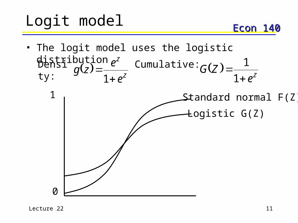
Econ 140Econ 140Logit model

• The logit model uses the logistic distribution

z

z

e

ezg

1

1

0

Standard normal F(Z)

Logistic G(Z)

Density: Cumulative: ze

ZG

1

1

Lecture 22 12

Econ 140Econ 140Maximum likelihood

• Alternative estimation that assumes you know the form of the population

• Using maximum likelihood, we will be specifying the model as part of the distribution

Lecture 22 13

Econ 140Econ 140Maximum likelihood (2)

• For example: Bernoulli distribution where: (with a parameter )

• We have an outcome

1 1 1 0 0 0 0 1 0 0

• The probability expression is:

• We pick a sample of Y1….Yn

4.0

111 64243

10Pr

1Pr

i

i

Y

Y

1)0Pr(

)1Pr(

Y

Y

Lecture 22 14

Econ 140Econ 140Maximum likelihood (3)

• Probability of getting observed Yi is based on the form we’ve assumed:

• If we multiply across the observed sample:

• Given we think that an outcome of one occurs r times:

ii YY 11

)1(

11 ii YY

n

i

)(ˆ1ˆ rnr

Lecture 22 15

Econ 140Econ 140Maximum likelihood (3)

• If we take logs, we get

– This is the log-likelihood

– We can differentiate this and obtain a solution for

ˆ1logˆlogˆ rnrL

Lecture 22 16

Econ 140Econ 140Maximum likelihood (4)

• In a more complex example, the logit model gives

• Instead of looking for estimates of we are looking for estimates of a and b

• Think of G(Zi) as :

– we get a log-likelihood

L(a, b) = i [Yi log(Gi) + (1 - Yi) log(1 - Gi)]

– solve for a and b

ii

ii

ii

ZGY

bXaZ

ZGY

10Pr

1Pr

Lecture 22 17

Econ 140Econ 140Example

• Data on union membership and years of labor market experience (L22.xls)

• To build the maximum likelihood form, we can think of:

– intercept: a

– coefficient on experience : b

• There are three columns

– Predicted value Z

– Estimated probability

– Estimated likelihood as given by the model

• The Solver from the Tools menu calculates estimates of a and b

Lecture 22 18

Econ 140Econ 140Example (2)

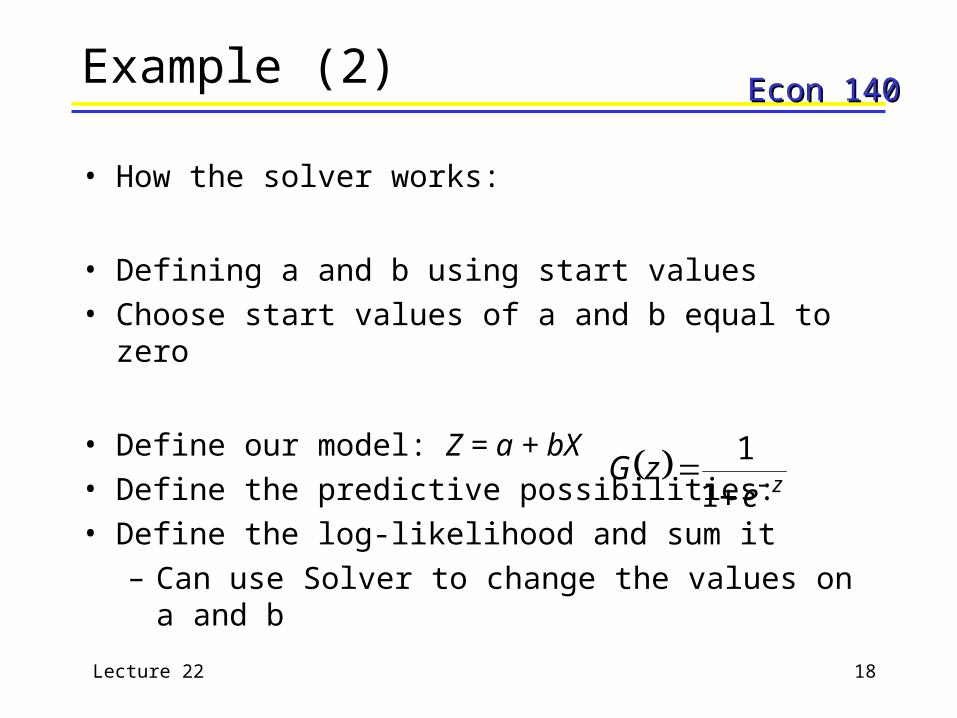
• How the solver works:

• Defining a and b using start values

• Choose start values of a and b equal to zero

• Define our model: Z = a + bX

• Define the predictive possibilities:

• Define the log-likelihood and sum it

– Can use Solver to change the values on a and b

ze

zG

1

1

Lecture 22 19

Econ 140Econ 140Comparing parameters

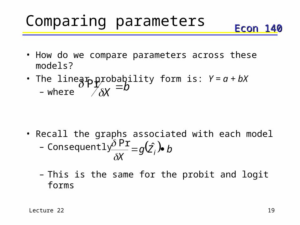
• How do we compare parameters across these models?

• The linear probability form is: Y = a + bX

– where

• Recall the graphs associated with each model

– Consequently

– This is the same for the probit and logit forms

bX Pr

bZgX i ˆPr

Lecture 22 20

Econ 140Econ 140L22.xls example

• Predicting the linear probability model:

• If we wanted to predict the probability given 20 years of experience, we’d have:

• For the logit form:

– use logit distribution:

– logit estimated equation is:

EXPERU 005.0281.0ˆ

291.020005.0281.0ˆ U

z

z

e

ezg

1

EXPERUZ 06.038.2ˆˆ

Lecture 22 21

Econ 140Econ 140L22.xls example (2)

• At 20 years of experience:

• Thus the slope at 20 years of experience is:

0.234 x 0.06 = 0.014

234.0307.01

307.0

307.0

18.12006.038.2ˆˆ

18.1ˆ

Zg

ee

UZZ