ECON 214 Elements of Statistics for Economists · 2017-02-22 · Elements of Statistics for Economists Session 6 – The Binomial and ... •A manufacturer claims a failure rate of

College of Education

School of Continuing and Distance Education 2014/2015 – 2016/2017

ECON 214

Elements of Statistics for

Economists

Session 6 – The Binomial and Poisson Distributions

Lecturer: Dr. Bernardin Senadza, Dept. of Economics Contact Information: [email protected]

Session Overview

• In this session, we discuss two standard discrete probability distributions; the Binomial and Poisson distributions.

• The Binomial distribution arises whenever the underlying probability experiment has just two possible outcome, e.g. heads or tails from the toss of a coin.

• On the other hand, the Poisson distribution describes rare events, when the probability of occurrence is low, e.g. the number of accidents on the Accra-Tema motorway in a day.

• We shall discuss these two discrete probabilities and compute probabilities for a possible number of occurrences of events.

Slide 2

Session Overview

• At the end of the session, the student will

– Be able to describe the characteristics and compute probabilities using the binomial distribution

– Be able to describe the characteristics and compute probabilities using the Poisson distribution

– Use the Poisson distribution to approximate the binomial distribution

Slide 3

Session Outline

The key topics to be covered in the session are as follows:

• Binomial probability distribution

• Poisson probability distribution

• Poisson approximation of the binomial probability distribution

Slide 4

Reading List

• Michael Barrow, “Statistics for Economics, Accounting and Business Studies”, 4th Edition, Pearson

• R.D. Mason , D.A. Lind, and W.G. Marchal, “Statistical Techniques in Business and Economics”, 10th Edition, McGraw-Hill

Slide 5

BINOMIAL PROBABILITY DISTRIBUTION

Topic One

Slide 6

The Binomial distribution

• The binomial distribution (BD) is applied when;

– Only two mutually exclusive outcomes are possible in each trial (success or failure)

– The outcomes in the series of trials are independent

– The probability of success, denoted P, in each trial remains constant from trial to trial

Slide 7


• The objective of using the BD is to determine the probability values for various possible number of successes (X);

– given the number of trails (n)

– and the known (and constant) probability of success (p).

Slide 8


• Consider five tosses of a coin.

• Recall from Session 5, we can write the probability of 1 Head in 2 tosses as the probability of a head and a tail (in that order) times the number of possible orderings (# of times that event occurs). – P (1 Head) = ½ ½ 2C1 = ¼ 2 = ½

• We can apply same technique to calculate the probability for the number of heads in five tosses of a coin.

Slide 9


• P (X Heads in five tosses of a coin) – P(X = 0) = (½)0 (½)5 5C0 = 1/32 1 = 1/32

– P(X = 1) = (½)1 (½)4 5C1 = 1/32 5 = 5/32

– P(X = 2) = (½)2 (½)3 5C2 = 1/32 10 = 10/32

– P(X = 3) = (½)3 (½)2 5C3 = 1/32 10 = 10/32

– P(X = 4) = (½)4 (½)1 5C4 = 1/32 5 = 5/32

– P(X = 5) = (½)5 (½)0 5C5 = 1/32 1 = 1/32

Slide 10


• To construct a binomial distribution, let – n be the number of trials – x be the number of observed successes – p be the probability of success on each trial

• the formula for the binomial probability distribution is:

Slide 11

!( ) (1 )

!( )!

n x n x

x

nP x C p p

x n x


• When the BD is used, it is typically because we wish to determine the probability of:

• “X or more” successes [ P(X ≥ xi) ]

• or

• “ X or fewer successes [P (X ≤ xi)]

• If the individual probabilities to be summed is large, it is easier to use the complement rule.

• Example: P (X ≥ xi) = 1 - P(X < xi)

Slide 12


• Suppose the probability is .05 that a randomly selected student of the University of Ghana owns a car. What is the probability of observing two or more student car-owners in a random sample of 20 students?

• P(X≥2) = P(X=2) + P(X=3) + …..+ P(X=20)

• P(X≥2) = 1 – P(X<2) = 1- P(X=0, 1)

• = 1 – [P(X=0) +P(X=1)]

• Now

– P(X=0) = 20C0 (.05)0(.95)20 = .3585

– P(X=1) = 20C1 (.05)(.95)19 = .3774

• So P(X≥2) = 1 – (.3585 + .3774) = .2641

Slide 13


• The mean of the binomial random variable is

E(X) = np

• And the variance is

σ2 = np(1-p)

• The standard deviation is the square root of the variance.

Slide 14

Slide 15

POISSON PROBABILITY DISTRIBUTION

• Topic Two

The Poisson distribution

• It is a sampling process in which events occur over time or space.

• The Poisson distribution is used to describe a number of processes or events such as

– The distribution of telephone calls going through a switch board

– The demand of patients for service at a health facility

– The arrival of vehicles at a tollbooth

– The number of accidents occurring at a road intersection, etc.

Slide 16


• Characteristics defining a Poisson random variable are

– The experiment consists of counting the number of times a particular event occurs during a given time interval

– The probability that the event occurs in one time interval is independent of the probability of the event occurring in another time interval

– The mean number of events in each unit of time is proportional to the length of the time interval.

Slide 17


• The probability that the Poisson random variable will assume the value X is given by

• For X = 0, 1, 2,3 ……. • λ is the mean of the distribution (mean number of

events occurring in a given unit of time) • e is approximately 2.7183 and is the base of the

natural logarithms. Slide 18

P!

xex

x


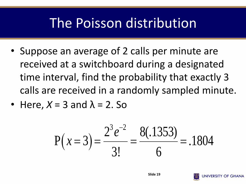
• Suppose an average of 2 calls per minute are received at a switchboard during a designated time interval, find the probability that exactly 3 calls are received in a randomly sampled minute.

• Here, X = 3 and λ = 2. So

Slide 19

3 22 8(.1353)

P 3 .18043! 6

ex


• As with the BD, the PD typically involves determining the probability of

• “X or more” number of events • or • “X or fewer” number of events. • To calculate, we sum the appropriate

probability values. • The use of the complement rule may also come

in handy.

Slide 20


• For example, we may want to calculate the probability of receiving 3 or more calls in a three-minute interval.

• That is P(X≥3) = P(X=3) + P(X=4) + … • Using the complement rule, we have • P(X≥3) = 1 - P(X<3) = 1 – [P(x=0) + P(x=1) +

P(x=2)] • From our proposition 3, we know the mean

number of occurrences is proportional to the length of the time interval.

Slide 21


• So if we expect a mean of 2 calls per minute, in three minutes we must expect 6 calls.

• For an interval of 30 seconds, the mean number of calls is one.

• The probability of 5 calls in a three-minute interval implies λ = 6, so P(X=5 / λ=6) = .1606

• The probability of no calls in an interval of 30 seconds implies that λ = 1, so P(X=0 / λ=1) = .3679

Slide 22


• The expected value and variance for a Poisson random variable are both equal to the mean number of events for the time interval of interest

• E (X) = λ

• Var (X) = λ

• The standard deviation is the square root of the variance.

Slide 23

POISSON APPROXIMATION OF THE BINOMIAL PROBABILITY

Topic Three

Slide 24

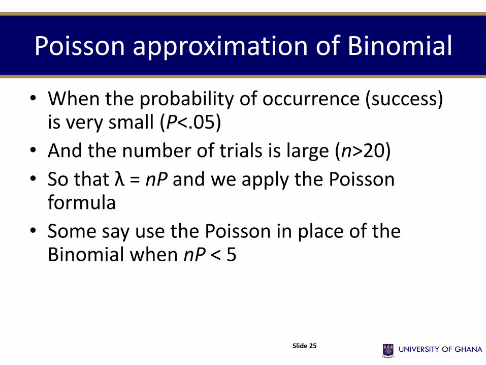
Poisson approximation of Binomial

• When the probability of occurrence (success) is very small (P<.05)

• And the number of trials is large (n>20)

• So that λ = nP and we apply the Poisson formula

• Some say use the Poisson in place of the Binomial when nP < 5

Slide 25


• A manufacturer claims a failure rate of 0.2% for its hard disk drives. In an assignment of 500 drives, what is the probability that, none are faulty, one is faulty, two are faulty?

• On average, 1 drive (0.2% of 500) should be faulty, so λ = nP = 1.

Slide 26


• The probability of no faulty drives is

• The probability of one faulty drive is

• The probability of two faulty drives is

Slide 27

0 11

P 0 0.3680!

ex

1 11

P 1 0.3681!

ex

2 11

P 2 0.1842!

ex

References

• Michael Barrow, “Statistics for Economics, Accounting and Business Studies”, 4th Edition, Pearson

• R.D. Mason , D.A. Lind, and W.G. Marchal, “Statistical Techniques in Business and Economics”, 10th Edition, McGraw-Hill

Slide 28

Documents

ECON 214 Elements of Statistics for Economists · 2017-02-22 · Elements of Statistics for Economists Session 6 – The Binomial and ... •A manufacturer claims a failure rate of