Embed Size (px)
Citation preview

Econ 704 Macroeconomic Theory Spring 2019∗
Jose-Vıctor Rıos-Rull
University of Pennsylvania
Federal Reserve Bank of Minneapolis
CAERP
May 15, 2019
∗This is the evolution of class notes by many students over the years, both from Penn and Minnesota including Makoto
Nakajima (2002), Vivian Zhanwei Yue (2002-3), Ahu Gemici (2003-4), Kagan (Omer Parmaksiz) (2004-5), Thanasis
Geromichalos (2005-6), Se Kyu Choi (2006-7), Serdar Ozkan (2007), Ali Shourideh (2008), Manuel Macera (2009),
Tayyar Buyukbasaran (2010), Bernabe Lopez-Martin (2011), Rishabh Kirpalani (2012), Zhifeng Cai (2013), Alexandra
(Sasha) Solovyeva (2014), Keyvan Eslami (2015), Sumedh Ambokar (2016), Omer Faruk Koru (2017), Jinfeng Luo
(2018), and Ricardo Marto (2019).
1
Contents
1 Introduction 6
2 Review: Neoclassical Growth Model 7
2.1 The Neoclassical Growth Model (Without Uncertainty) . . . . . . . . . . . . . . . . . 7
2.2 A Comment on the Welfare Theorems . . . . . . . . . . . . . . . . . . . . . . . . . . 10
3 Recursive Competitive Equilibrium 10
3.1 A Simple Example . . . . . . . . . . . . . . . . . . . . . . . . . . . . . . . . . . . . 10
3.2 The Envelope Theorem and the Functional Euler equation . . . . . . . . . . . . . . . 13
3.3 Economies with Government Expenditures . . . . . . . . . . . . . . . . . . . . . . . 15
3.3.1 Lump-Sum Tax . . . . . . . . . . . . . . . . . . . . . . . . . . . . . . . . . 15
3.3.2 Labor Income Tax . . . . . . . . . . . . . . . . . . . . . . . . . . . . . . . . 16
3.3.3 Capital Income Tax . . . . . . . . . . . . . . . . . . . . . . . . . . . . . . . 17
3.3.4 Taxes and Debt . . . . . . . . . . . . . . . . . . . . . . . . . . . . . . . . . 17
4 Some Other Examples 19
4.1 A Few Popular Utility Functions . . . . . . . . . . . . . . . . . . . . . . . . . . . . . 19
4.2 An Economy with Capital and Land . . . . . . . . . . . . . . . . . . . . . . . . . . . 20
2

5 Adding Heterogeneity 22
5.1 Heterogeneity in Wealth . . . . . . . . . . . . . . . . . . . . . . . . . . . . . . . . . 22
5.2 Heterogeneity in Skills . . . . . . . . . . . . . . . . . . . . . . . . . . . . . . . . . . 25
5.3 An International Economy Model . . . . . . . . . . . . . . . . . . . . . . . . . . . . 26
6 Stochastic Economies 28
6.1 A Review . . . . . . . . . . . . . . . . . . . . . . . . . . . . . . . . . . . . . . . . . 28
6.1.1 Markov Processes . . . . . . . . . . . . . . . . . . . . . . . . . . . . . . . . 28
6.1.2 Problem of the Social Planner . . . . . . . . . . . . . . . . . . . . . . . . . . 29
6.1.3 Recursive Competitive Equilibrium . . . . . . . . . . . . . . . . . . . . . . . . 32
6.2 An International Economy Model with Shocks . . . . . . . . . . . . . . . . . . . . . 33
6.3 Heterogeneity in Wealth and Skills with Complete Markets . . . . . . . . . . . . . . . 35
7 Asset Pricing: Lucas Tree Model 37
7.1 The Lucas Tree with Random Endowments . . . . . . . . . . . . . . . . . . . . . . . 37
7.2 Asset Pricing . . . . . . . . . . . . . . . . . . . . . . . . . . . . . . . . . . . . . . . 39
7.3 Taste Shocks . . . . . . . . . . . . . . . . . . . . . . . . . . . . . . . . . . . . . . . 41
8 Endogenous Productivity in a Product Search Model 42
8.1 Competitive Search . . . . . . . . . . . . . . . . . . . . . . . . . . . . . . . . . . . 44
3
8.1.1 Firms’ Problem . . . . . . . . . . . . . . . . . . . . . . . . . . . . . . . . . . 49
9 Measure Theory 49
10 Industry Equilibrium 55
10.1 Preliminaries . . . . . . . . . . . . . . . . . . . . . . . . . . . . . . . . . . . . . . . 55
10.2 A Simple Dynamic Environment . . . . . . . . . . . . . . . . . . . . . . . . . . . . . 56
10.3 Introducing Exit Decisions . . . . . . . . . . . . . . . . . . . . . . . . . . . . . . . . 59
10.4 Stationary Equilibrium . . . . . . . . . . . . . . . . . . . . . . . . . . . . . . . . . . 63
10.5 Adjustment Costs . . . . . . . . . . . . . . . . . . . . . . . . . . . . . . . . . . . . 65
10.6 Non-stationary Equilibrium . . . . . . . . . . . . . . . . . . . . . . . . . . . . . . . . 67
10.7 Linear Approximation . . . . . . . . . . . . . . . . . . . . . . . . . . . . . . . . . . 69
11 Incomplete Market Models 71
11.1 A Farmer’s Problem . . . . . . . . . . . . . . . . . . . . . . . . . . . . . . . . . . . 71
11.2 Huggett Economy . . . . . . . . . . . . . . . . . . . . . . . . . . . . . . . . . . . 74
11.3 Aiyagari Economy . . . . . . . . . . . . . . . . . . . . . . . . . . . . . . . . . . . 76
11.3.1 Policy Changes and Welfare . . . . . . . . . . . . . . . . . . . . . . . . . . . 79
11.4 Business Cycles in an Aiyagari Economy . . . . . . . . . . . . . . . . . . . . . . . . . 80
11.4.1 Aggregate Shocks . . . . . . . . . . . . . . . . . . . . . . . . . . . . . . . . 80
4

11.4.2 Linear Approximation Revisited . . . . . . . . . . . . . . . . . . . . . . . . . 82
11.5 Aiyagari Economy with Job Search . . . . . . . . . . . . . . . . . . . . . . . . . . . 83
11.6 Aiyagari Economy with Entrepreneurs . . . . . . . . . . . . . . . . . . . . . . . . . . 84
11.7 Other Extensions . . . . . . . . . . . . . . . . . . . . . . . . . . . . . . . . . . . . . 86
12 Monopolistic Competition 87
12.1 Benchmark Monopolistic Competition . . . . . . . . . . . . . . . . . . . . . . . . . . 87
12.2 Price Rigidity . . . . . . . . . . . . . . . . . . . . . . . . . . . . . . . . . . . . . . . 90
A A Farmer’s Problem: Revisited 92
5

1 Introduction
A model is an artificial economy. The description of a model’s environment may include specifying
the agents’ preferences and endowment, technology available, information structure as well as property
rights. The Neoclassical Growth Model is one of the workhorses of modern macroeconomics because it
delivers some fundamental properties of industrialized economies, summarized by, among others, Kaldor
(1957):
1. Output per capita has grown at a roughly constant rate (2%).
2. The capital-output ratio (where capital is measured using the perpetual inventory method based
on past consumption foregone) has remained roughly constant (despite output per capita growth).
3. The capital-labor ratio has grown at a roughly constant rate equal to the growth rate of output.
4. The wage rate has grown at a roughly constant rate equal to the growth rate of output.
5. The real interest rate has been stationary and, during long periods, roughly constant.
6. Labor income as a share of output has remained roughly constant (0.66).
7. Hours worked per capita have been roughly constant.
Equilibrium can be defined as a prediction of what will happen and therefore it is a mapping from
environments to outcomes (allocations, prices, etc.). One equilibrium concept that we will deal with is
Competitive Equilibrium.1 Characterizing the equilibrium, however, usually involves finding solutions to
a system of an infinite number of equations. There are generally two ways of getting around this. First,
invoke the welfare theorem to solve for the allocation and then find the equilibrium prices associated
with it. This may sometimes not work due to, say, the presence of externalities. The second way is to
resort to dynamic programming and study a Recursive Competitive equilibrium, in which equilibrium
objects are functions instead of variables.
1 Arrow-Debreu or Valuation Equilibrium.
6

2 Review: Neoclassical Growth Model
We review briefly the basic neoclassical growth model.
2.1 The Neoclassical Growth Model (Without Uncertainty)
The commodity space is
L = (l1, l2, l3) : li = (lit)∞t=0 lit ∈ R, sup
t|lit|<∞, i = 1, 2, 3.
The consumption possibility set is
X(k0) = x ∈ L : ∃(ct, kt+1)∞t=0 s.th. ∀t = 0, 1, . . .
ct, kt+1 ≥ 0, x1t + (1− δ)kt = ct + kt+1, −kt ≤ x2t ≤ 0, −1 ≤ x3t ≤ 0, k0 = k0.
The production possibility set is Y =∏
t Yt, where
Yt = (y1t, y2t, y3t) ∈ R3 : 0 ≤ y1t ≤ F (−y2t,−y3t).
Definition 1 An Arrow-Debreu equilibrium is (x∗, y∗) ∈ X ×Y , and a continuous linear functional ν∗
such that
1. x∗ ∈ arg maxx∈X,ν∗(x)≤0
∑∞t=0 β
tu(ct(x),−x3t),
2. y∗ ∈ arg maxy∈Y ν∗(y),
3. and x∗ = y∗.
Note that in this definition we have added leisure. Now, let’s look at the one-sector growth model’s
7
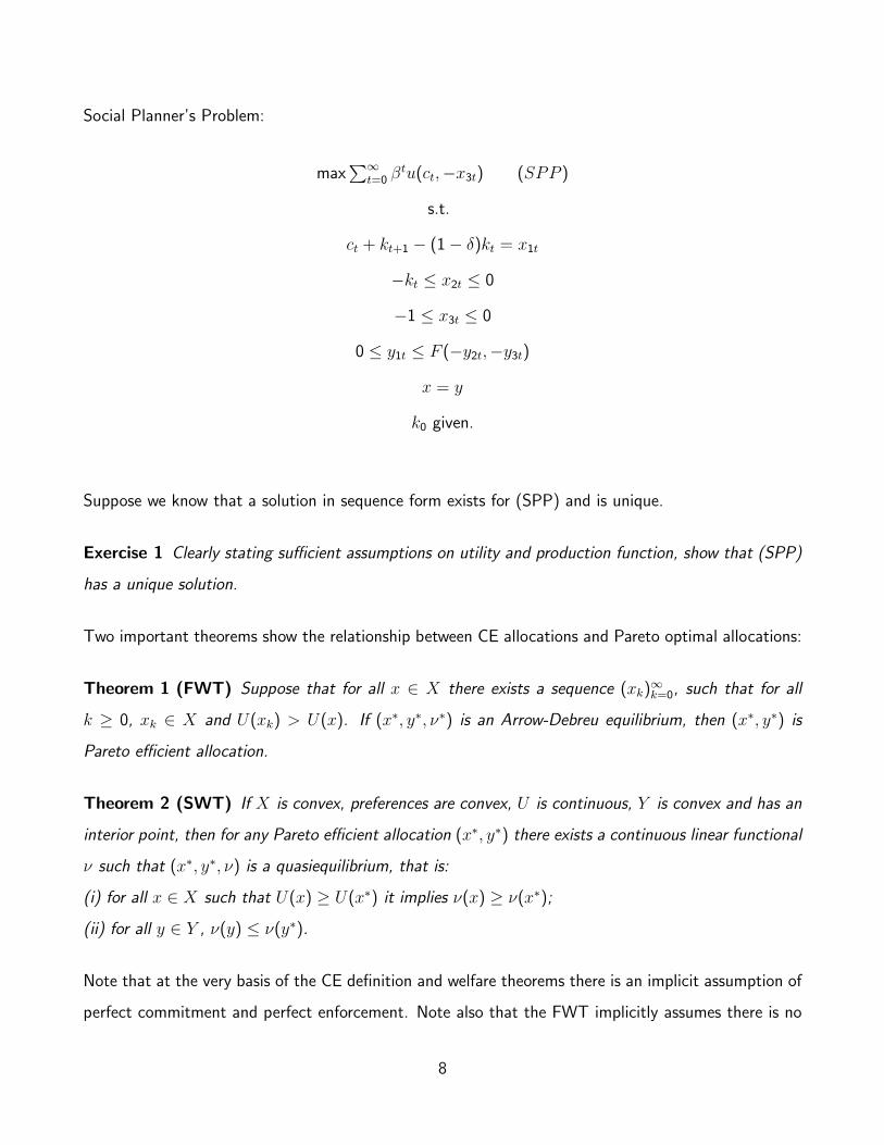
Social Planner’s Problem:
max∑∞
t=0 βtu(ct,−x3t) (SPP )
s.t.
ct + kt+1 − (1− δ)kt = x1t
−kt ≤ x2t ≤ 0
−1 ≤ x3t ≤ 0
0 ≤ y1t ≤ F (−y2t,−y3t)
x = y
k0 given.
Suppose we know that a solution in sequence form exists for (SPP) and is unique.
Exercise 1 Clearly stating sufficient assumptions on utility and production function, show that (SPP)
has a unique solution.
Two important theorems show the relationship between CE allocations and Pareto optimal allocations:
Theorem 1 (FWT) Suppose that for all x ∈ X there exists a sequence (xk)∞k=0, such that for all
k ≥ 0, xk ∈ X and U(xk) > U(x). If (x∗, y∗, ν∗) is an Arrow-Debreu equilibrium, then (x∗, y∗) is
Pareto efficient allocation.
Theorem 2 (SWT) If X is convex, preferences are convex, U is continuous, Y is convex and has an
interior point, then for any Pareto efficient allocation (x∗, y∗) there exists a continuous linear functional
ν such that (x∗, y∗, ν) is a quasiequilibrium, that is:
(i) for all x ∈ X such that U(x) ≥ U(x∗) it implies ν(x) ≥ ν(x∗);
(ii) for all y ∈ Y , ν(y) ≤ ν(y∗).
Note that at the very basis of the CE definition and welfare theorems there is an implicit assumption of
perfect commitment and perfect enforcement. Note also that the FWT implicitly assumes there is no
8

externality or public goods (achieves this implicit assumption by defining a consumer’s utility function
only on his own consumption set but no other points in the commodity space). The Greenwald-
Stiglitz theorem establishes the Pareto inefficiency of market economies with imperfect information and
incomplete markets.
From the First Welfare Theorem, we know that if a Competitive Equilibrium exists, it is Pareto Optimal.
Moreover, if the assumptions of the Second Welfare Theorem are satisfied and if the SPP has a unique
solution, then the competitive equilibrium allocation is unique and is the same as the PO allocation.
Prices can be constructed using this allocation and first-order conditions.
Exercise 2 Show that
v2t
v1t= Fk(kt, lt) and
v3t
v1t= Fl(kt, lt).
One shortcoming of the AD equilibrium is that all trade occurs at the beginning of time. This assump-
tion is unrealistic. Modern economics is based on sequential markets. Therefore, we define another
equilibrium concept, Sequential Markets Equilibrium (SME). We can easily show that SME is equivalent
to ADE by introducing AD securities. All of our results still hold and SME is the right problem to solve.
Exercise 3 Define a Sequential Markets Equilibrium (SME) for this economy. Prove that the objects
we get from the AD equilibrium satisfy SME conditions and that the converse is also true. We should
first show that a CE exists and therefore coincides with the unique solution of (SPP).
Note that the (SPP) problem is hard to solve, since we are dealing with an infinite number of choice
variables. We have already established the fact that this SPP problem is equivalent to the following
dynamic problem (removing leisure from now on), which is easier to solve:
v(k) = maxc,k′
u(c) + βv(k′) (RSPP )
s.t. c + k′ = f(k).
9
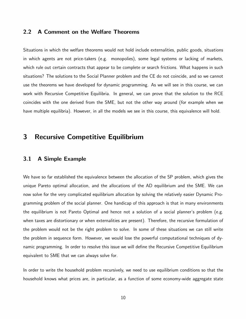
2.2 A Comment on the Welfare Theorems
Situations in which the welfare theorems would not hold include externalities, public goods, situations
in which agents are not price-takers (e.g. monopolies), some legal systems or lacking of markets,
which rule out certain contracts that appear to be complete or search frictions. What happens in such
situations? The solutions to the Social Planner problem and the CE do not coincide, and so we cannot
use the theorems we have developed for dynamic programming. As we will see in this course, we can
work with Recursive Competitive Equilibria. In general, we can prove that the solution to the RCE
coincides with the one derived from the SME, but not the other way around (for example when we
have multiple equilibria). However, in all the models we see in this course, this equivalence will hold.
3 Recursive Competitive Equilibrium
3.1 A Simple Example
We have so far established the equivalence between the allocation of the SP problem, which gives the
unique Pareto optimal allocation, and the allocations of the AD equilibrium and the SME. We can
now solve for the very complicated equilibrium allocation by solving the relatively easier Dynamic Pro-
gramming problem of the social planner. One handicap of this approach is that in many environments
the equilibrium is not Pareto Optimal and hence not a solution of a social planner’s problem (e.g.
when taxes are distortionary or when externalities are present). Therefore, the recursive formulation of
the problem would not be the right problem to solve. In some of these situations we can still write
the problem in sequence form. However, we would lose the powerful computational techniques of dy-
namic programming. In order to resolve this issue we will define the Recursive Competitive Equilibrium
equivalent to SME that we can always solve for.
In order to write the household problem recursively, we need to use equilibrium conditions so that the
household knows what prices are, in particular, as a function of some economy-wide aggregate state
10

variables. Let aggregate capital be K and aggregate labor L = 1. Then from solving the firm’s problem,
factor prices are given by w (K) = Fn (K, 1) and R (K) = Fk (K, 1). Therefore, since households take
prices as given, they need to know aggregate capital. A household who is deciding about how much
to consume and how much to work has to know the whole sequence of future prices in order to make
her decision and that means that she needs to know the path of aggregate capital. Therefore, if she
believes that aggregate capital changes according to the mapping G such that K ′ = G(K), then
knowing aggregate capital today she would be able to project the path of aggregate capital into the
future and thus the path for prices. So, we can write the household problem given function G(·) as
follows:
Ω(K, a;G) = maxc,a′
u(c) + βΩ(K ′, a′;G) (RCE)
s.t. c + a′ = w(K) + R(K)a
K ′ = G(K),
c ≥ 0
The above problem is the problem of a household that sees K in the economy, has a belief G about its
evoluation, and carries a units of assets from past. The solution of this problem yields policy functions
c(K, a;G) for consumption and g(K, a;G) for next period asset holdings, as well as a value function
Ω(K, a;G). The price functions w(K), R(K) are obtained from the firm’s FOCs (below).
uc (c(K, a;G)) = βΩa′ (G(K), g(K, a;G);G)
Ωa (K, a;G) = R(K) uc (c(K, a;G))
Now we can define the Recursive Competitive Equilibrium.
Definition 2 A Recursive Competitive Equilibrium with arbitrary expectations G is a set of functions
Ω, g : K ×A → R, and R, w, H : K → R+ such that:2
2 Note that we could add the policy function for consumption c(K, a;G).
11
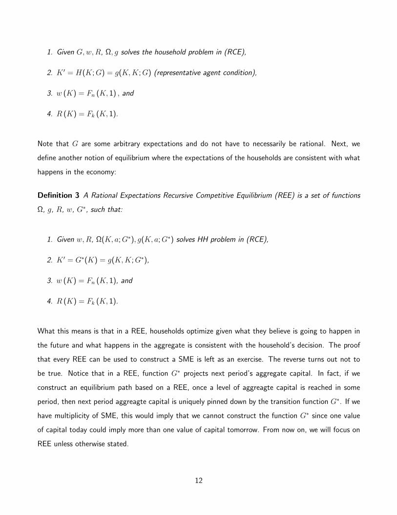
1. Given G,w,R, Ω, g solves the household problem in (RCE),
2. K ′ = H(K;G) = g(K,K;G) (representative agent condition),
3. w (K) = Fn (K, 1) , and
4. R (K) = Fk (K, 1).
Note that G are some arbitrary expectations and do not have to necessarily be rational. Next, we
define another notion of equilibrium where the expectations of the households are consistent with what
happens in the economy:
Definition 3 A Rational Expectations Recursive Competitive Equilibrium (REE) is a set of functions
Ω, g, R, w, G∗, such that:
1. Given w,R, Ω(K, a;G∗), g(K, a;G∗) solves HH problem in (RCE),
2. K ′ = G∗(K) = g(K,K;G∗),
3. w (K) = Fn (K, 1), and
4. R (K) = Fk (K, 1).
What this means is that in a REE, households optimize given what they believe is going to happen in
the future and what happens in the aggregate is consistent with the household’s decision. The proof
that every REE can be used to construct a SME is left as an exercise. The reverse turns out not to
be true. Notice that in a REE, function G∗ projects next period’s aggregate capital. In fact, if we
construct an equilibrium path based on a REE, once a level of aggreagte capital is reached in some
period, then next period aggreagte capital is uniquely pinned down by the transition function G∗. If we
have multiplicity of SME, this would imply that we cannot construct the function G∗ since one value
of capital today could imply more than one value of capital tomorrow. From now on, we will focus on
REE unless otherwise stated.
12

Remark 1 Note that unless otherwise stated, we will assume that the capital depreciation rate δ is 1,
with the firm’s profits given by F (K, 1)− δK − r(K)K −w(K). R (K) is the gross rate of return on
capital, which is given by Fk (K, 1) + 1− δ. The net rate of return on capital is r (K) = Fk (K, 1)− δ.
3.2 The Envelope Theorem and the Functional Euler equation
To solve for the RCE and, in particular, to derive the household’s optimality conditions we use envelope
theorem. This method is valid because of time consistency of consumption choice.
Take the household’s problem given by
V (K, a) = maxc,a′
u(c) + βV (K ′, a′)
s.t. c + a′ = w(K) + R(K)a
K ′ = G(K)
c ≥ 0
with decision rules for consumption and next period asset holdings given by c = c(K, a) and a′ =
g(K, a).
By taking the first-order conditions (assuming an interior solution since u is well behaved), we get:
−uc(c) + βVa′(K′, a′) = 0,
which evaluated at the optimum is
−uc (w(K) + R(K)a− g(K, a)) + βVa′ (G(K), g(K, a)) = 0 (1)
The problem with solving the functional Euler equation is that Va′ is not known. However, we can
13
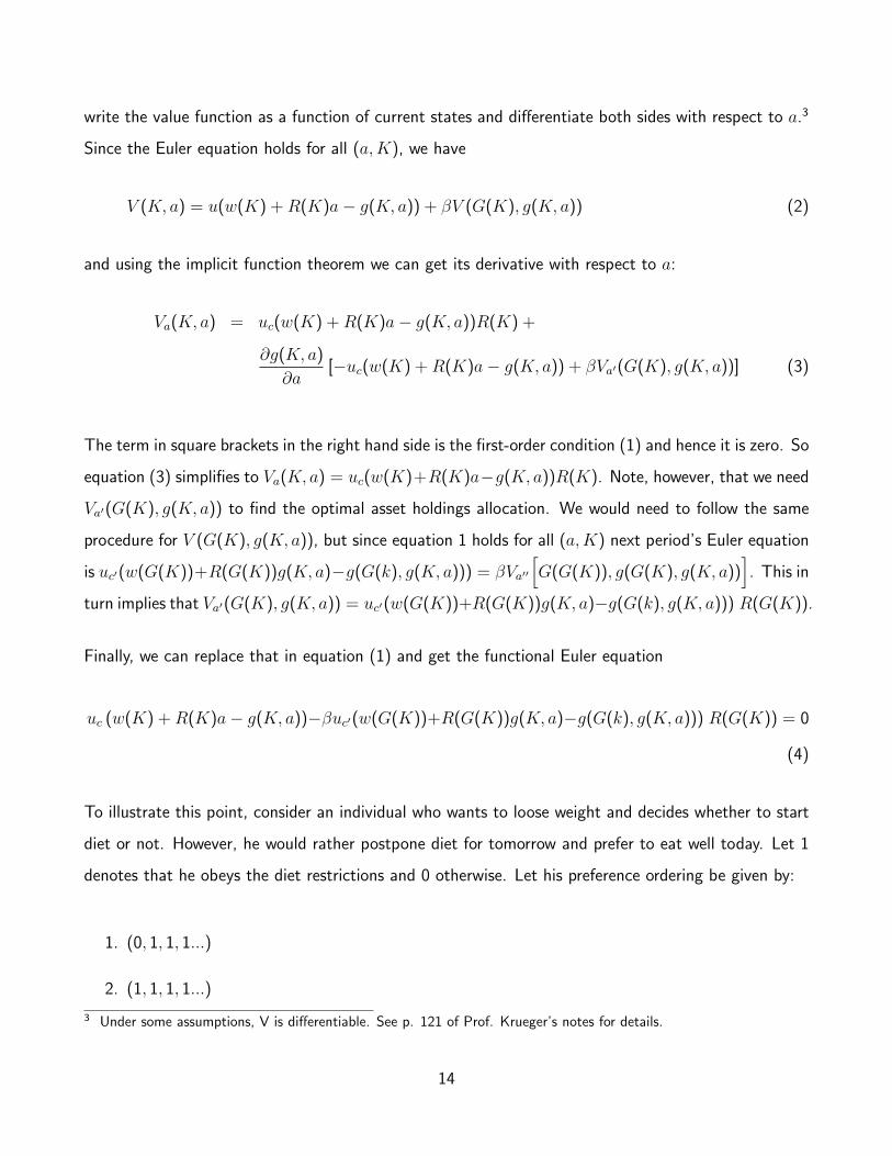
write the value function as a function of current states and differentiate both sides with respect to a.3
Since the Euler equation holds for all (a,K), we have
V (K, a) = u(w(K) + R(K)a− g(K, a)) + βV (G(K), g(K, a)) (2)
and using the implicit function theorem we can get its derivative with respect to a:
Va(K, a) = uc(w(K) + R(K)a− g(K, a))R(K) +
∂g(K, a)
∂a[−uc(w(K) + R(K)a− g(K, a)) + βVa′(G(K), g(K, a))] (3)
The term in square brackets in the right hand side is the first-order condition (1) and hence it is zero. So
equation (3) simplifies to Va(K, a) = uc(w(K)+R(K)a−g(K, a))R(K). Note, however, that we need
Va′(G(K), g(K, a)) to find the optimal asset holdings allocation. We would need to follow the same
procedure for V (G(K), g(K, a)), but since equation 1 holds for all (a,K) next period’s Euler equation
is uc′(w(G(K))+R(G(K))g(K, a)−g(G(k), g(K, a))) = βVa′′[G(G(K)), g(G(K), g(K, a))
]. This in
turn implies that Va′(G(K), g(K, a)) = uc′(w(G(K))+R(G(K))g(K, a)−g(G(k), g(K, a))) R(G(K)).
Finally, we can replace that in equation (1) and get the functional Euler equation
uc (w(K) + R(K)a− g(K, a))−βuc′(w(G(K))+R(G(K))g(K, a)−g(G(k), g(K, a))) R(G(K)) = 0
(4)
To illustrate this point, consider an individual who wants to loose weight and decides whether to start
diet or not. However, he would rather postpone diet for tomorrow and prefer to eat well today. Let 1
denotes that he obeys the diet restrictions and 0 otherwise. Let his preference ordering be given by:
1. (0, 1, 1, 1...)
2. (1, 1, 1, 1...)
3 Under some assumptions, V is differentiable. See p. 121 of Prof. Krueger’s notes for details.
14

3. (0, 0, 0, 0, ...)
Even though he promises himself that he will start diet tomorrow and chooses to eat well today,
tomorrow he will face the same problem. So he will choose the same option again tomorrow. He will
thus never start diet and will end up with his least preferred option: (0, 0, 0, 0, ...).
However, in our model that is not what happens. Agents’ preferences are time consistent, so what an
individual promises today has to be optimal for her tomorrow as well. And that is why we can use the
envelope theorem.
3.3 Economies with Government Expenditures
3.3.1 Lump-Sum Tax
The government levies each period T units of goods in a lump sum fashion and spends it in a public
good, say, medals. Assume however that consumers do not care about medals. The household’s
problem is
V (K, a) = maxc,a′
u(c) + βV (K ′, a′)
s.t. c + a′ = w(K) + R(K)a− T
K ′ = G(K)
c ≥ 0
Let the solution of this problem be given by policy function ga(K, a;M,T ) and value function V (K, a;M,T ).
The equilibrium can be characterized by G∗(K;M,T ) = ga(K,K;G∗,M, T ) and M∗ = T (the govern-
ment budget constraint is balanced period by period). We will write a complete definition of equilibrium
for a version with government debt (below).
Exercise 4 Define the aggregate resource constraint as C +K ′+M = f(K, 1) for the planner. Show
15

that the equilibrium is optimal when consumers do not care about medals.
Note that if households cared about medals, then the equilibrium would not necessarily be optimal.
The social planner would equate the marginal utility of consumption and of medals, while the agent
would not.
3.3.2 Labor Income Tax
We have an economy in which the government levies a tax on labor income in order to purchase medals.
Medals are goods that provide utility to the consumers.
V (K, a) = maxc,a′
u(c,M) + βV (K ′, a′)
s.t. c + a′ = (1− τ(K))w(K) + R(K)a
K ′ = G(K)
c ≥ 0
with M = τ(K)w (K).
Since leisure is not valued, the labor decision is trivial. Hence, there is no distortion due to taxes and
the CE is Pareto optimal.
Exercise 5 Is there any change in the above implications of optimality if the tax rate is a function of
aggregate capital?
Exercise 6 Suppose medals do not provide utility to agents but leisure does. Is the CE optimal now?
Is it distorted? What if medals also provide utility?
16

3.3.3 Capital Income Tax
Now let us look at an economy in which the government levies tax on capital in order to purchase
medals. Medals provide utility to the consumers.
V (K, a) = maxc,a′
u(c,M) + βV (K ′, a′)
s.t. c + a′ = w(K) + a [1 + r(K) (1− τ(K))]
K ′ = G(K)
c ≥ 0
with M = τ(K)r (K)K and R (K) = 1 + r (K). Now, the First Welfare Theorem is no longer
applicable and the CE will therefore not be Pareto optimal anymore (if τ(K) > 0 there will be a wedge,
and the efficiency conditions will not be satisfied).
Exercise 7 Derive the first order conditions in the above problem to see the wedge introduced by
taxes.
3.3.4 Taxes and Debt
Assume that the government can now issue debt and use taxes to finance its expenditures. Also assume
that agents derive utility from these government expenditures.
A government policy consists of capital taxes, spending (medals) as well as bond issuance. When the
aggregate states are K and B, as you will see why, then a government policy (in a recursive world) is
τ (K,B) , M (K,B) and B′ (K,B) .
For now, we shall assume these values are chosen so that the equilibrium exists. In this environment,
debt issued is relevant for the household because it permits him to correctly infer the amount of taxes.
Therefore the household needs to form expectations about the future level of debt from the government.
17

The government budget constraint now satisfies (with taxes on labor income):
B + M(K,B) = τ(K,B)R(K)K + q(K,B)B′(K,B)
Notice that the household does not care about the composition of his portfolio as long as assets have
the same rate of return, which is true because of the no arbitrage condition.
The problem of a household with assets a is given by:
V (K,B, a) = maxc,a′
u(c,M(K,B)) + βV (K ′, B′, a′)
s.t. c + a′ = w(K) + aR(K) (1− τ(K,B))
K ′ = G(K,B)
B′ = H(K,B)
c ≥ 0
Let g (K,B, a) be the policy function associated with this problem. Then, we can define a RCE as
follows.
Definition 4 A Rational Expectations Recursive Competitive Equilibrium, given policies M(K,B) and
τ(K,B), is a set of functions V , g, G, H, w, and R, such that
1. Given w and R, V and g solve the household’s problem,
2. Factor prices are paid their marginal productivities
w(K) = F2(K, 1) and R(K) = F1(K, 1),
3. Household wealth = Aggregate wealth
g(K,B,K + q(K−, B−)B) = G(K,B) + q(K,B)H(K,B),
18
4. No arbitrage condition
1
q(K,B)= [1− τ(G(K,B), H(K,B))]R(G(K)),
5. Government’s budget constraint holds
B + M(K,B) = τ(K,B)R(K)K + q(K,B)H(K,B),
6. Government debt is bounded; i.e. ∃ some B, such that for all K ∈[
0, k)
and B ≤ B,
H (K,B) ≤ B.
4 Some Other Examples
4.1 A Few Popular Utility Functions
Consider the following three utility forms:
1. u (c, c−): this function is called habit formation utility function. The utility is increasing in
consumption today, but decreasing in the deviations from past consumption (e.g. u (c, c−) =
v (c) − (c− c−)2). Under habit persistence, an increase in current consumption lowers the
marginal utility of consumption in the current period (u′′1,1 < 0) and increases it in the next
period (u′′1,2 > 0). Intuitively, the more the agent eats today, the hungrier she will be tomorrow.
The aggregate state in this setup is K, while the individual states are a and c−.
Definition 5 A Recursive Competitive Equilibrium is a set of functions V , g, G, w, and R, such
that
(a) Given w and R, V and g solve the household’s problem,
19
(b) Factor prices are paid their marginal productivities
w(K) = F2(K, 1) and R(K) = F1(K, 1),
(c) Household wealth = Aggregate wealth
g(K,K,F (G−1(K), 1)−K) = G(K).
Exercise 8 Is the equilibrium optimum in this case?
2. u (c, C−): this form is called catching up with Jones. There is an externality from aggregate
consumption to the agent’s payoff. Intuitively, agents care about what their neighbors consume.
The aggregate states in this case are K and C−, while c− is no longer an individual state.
Exercise 9 How does the agent know C?
Exercise 10 Is the equilibrium optimum in this case?
3. u (c, C): this form is called keeping up with Jones. The aggregate state is K and C is no longer
a predetermined variable.
Exercise 11 How does the agent know C?
Exercise 12 Is the equilibrium optimum in this case?
4.2 An Economy with Capital and Land
Consider an economy with capital and land but without labor. A firm in this economy buys and installs
capital, and owns one unit of land that is used in production, according to the technology F (K,L). In
other words, a firm is a “chunk of land of area one” (e.g. farmland), in which it installs its own capital
(e.g. tractors). The firm’s shares are traded in a stock market, which are bought by households.
20

A household’s problem in this economy is given by:
V (K, a) = maxc,a′
u(c) + βV (K ′, a′)
s.t. c + P (K)a′ = a [D(K) + P (K)]
K ′ = G(K)
where a are shares held by the household, P (K) is their price, and D(K) are dividends per share.
The firm’s problem is given by
Ω(K, k) = maxd,k′
d + q(K ′)Ω(K ′, k′)
s.t. f(k′, 1) = d + k′
K ′ = G(K)
Ω here is the value of the firm, measured in units of output today. The value of the firm tomorrow
must be discounted into units of output today, which is done by the discount factor q (K ′). Note that
the firm needs to know K ′, using the aggregate law of motion G to do so.
Definition 6 A Recursive Competitive Equilibrium consists of functions, V , Ω, h, g, d, q, D, P , and
G so that:
1. Given prices, V and h solve the household’s problem,
2. Ω, g, and d solve the firm’s problem,
3. Representative household holds all shares of the firm
g(K, 1) = 1,
4. The capital of the firm when it is representative must equal the aggregate stock of capital
h(K,K) = G(K),
21
5. Value of a representative firm must equal its price and dividends
Ω(K,K) = D(K) + P (K),
6. The dividends of the representative firm must equal aggregate dividends
d(K,K) = D(K)
Exercise 13 One condition is missing in the definition of the RCE above. Find it! [Hint: it relates the
discount factor of the firm q(G(K)) with the price and dividends households receive (P (K), P (G(K)),
and D(G(K))).]
Exercise 14 Define the RCE if a were savings paying R(K) as opposed to shares of the firm.
5 Adding Heterogeneity
In the previous section we looked at situations in which recursive competitive equilibria (RCE) were
useful. In particular these were situations in which the welfare theorems failed and so we could not use
the standard dynamic programming techniques learned earlier. In this section we look at another way
in which RCE are helpful, in particular in models with heterogeneous agents.
5.1 Heterogeneity in Wealth
First, let us consider a model in which we have two types of households that differ only in the amount
of wealth they own. Say there are two types of agents, labeled type R (for rich) and P (for poor),
of measure µ and 1 − µ respectively. Agents are identical other than their initial wealth position and
22
there is no uncertainty in the model. The problem of an agent with wealth a is given by
V (KR, KP , a) = maxc,a′
u(c) + βV (KR′ , KP ′ , a′)
s.t. c + a′ = w(µKR + (1− µ)KP ) + aR(µKR + (1− µ)KP )
Ki′ = Gi(KR, KP ) for i = R,P.
Remark 2 Note that (in general) the decision rules of the two types of agents are not linear (even
though they might be almost linear); therefore, we cannot add the two states, K1 and K2, to write
the problem with one aggregate state, in the recursive form.
Definition 7 A Recursive Competitive Equilibrium is a set of functions V , g, w, R, G1, and G2 such
that that:
1. Given prices, V solves the household’s functional equation, with g as the associated policy func-
tion,
2. w and R are the marginal products of labor and capital, respectively (watch out for arguments!),
3. Consistency: representative agent conditions are satisfied, i.e.
g(KR, KP , KR) = GR(KR, KP ),
and
g(KR, KP , KP ) = GP (KR, KP ).
Remark 3 Note that GR(KR, KP
)= GP
(KP , KR
)(look at the arguments carefully). Why? (How
are rich and poor different?)
Remark 4 This is a variation of the simple neoclassical growth model. What does the neoclassical
growth model say about inequality? In the steady state, the Euler equations for the two different types
23
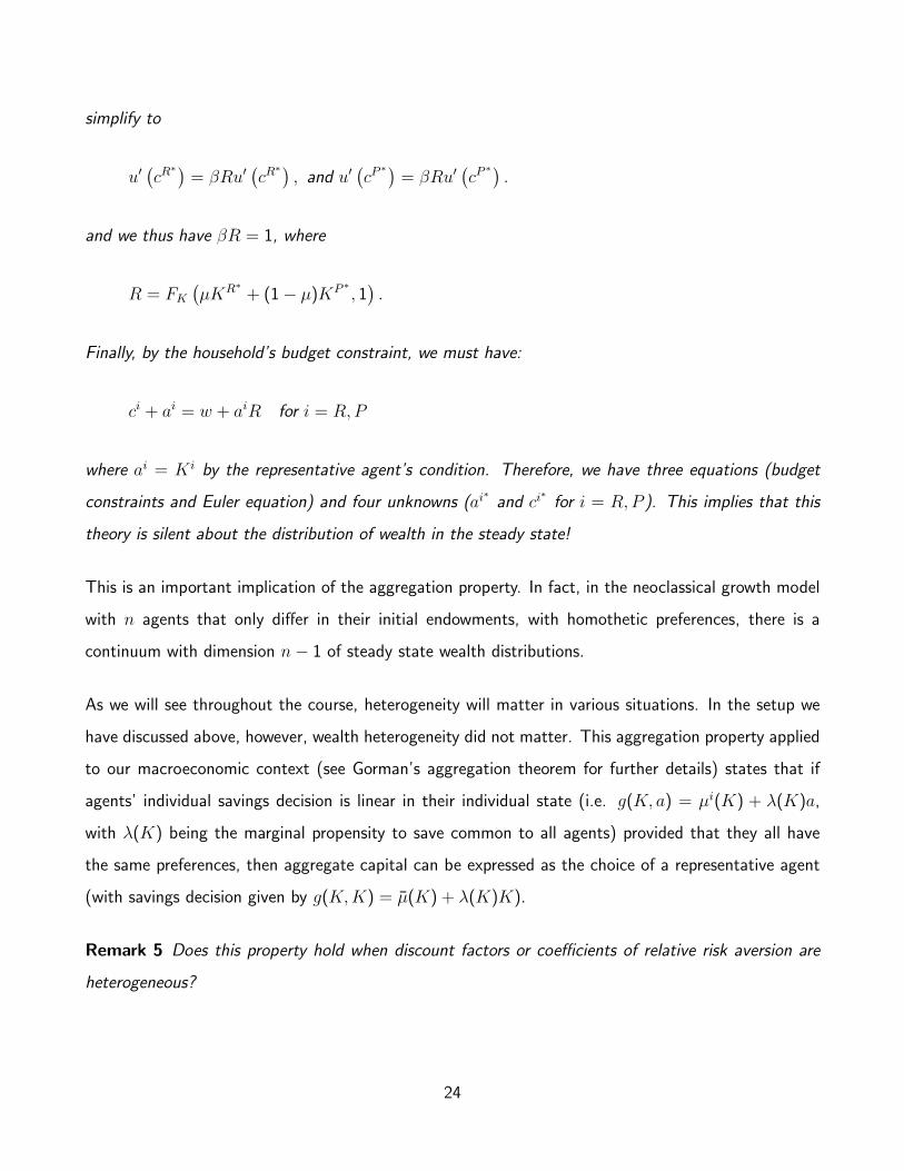
simplify to
u′(cR∗)
= βRu′(cR∗), and u′
(cP∗)
= βRu′(cP∗).
and we thus have βR = 1, where
R = FK(µKR∗ + (1− µ)KP ∗ , 1
).
Finally, by the household’s budget constraint, we must have:
ci + ai = w + aiR for i = R,P
where ai = Ki by the representative agent’s condition. Therefore, we have three equations (budget
constraints and Euler equation) and four unknowns (ai∗
and ci∗
for i = R,P ). This implies that this
theory is silent about the distribution of wealth in the steady state!
This is an important implication of the aggregation property. In fact, in the neoclassical growth model
with n agents that only differ in their initial endowments, with homothetic preferences, there is a
continuum with dimension n− 1 of steady state wealth distributions.
As we will see throughout the course, heterogeneity will matter in various situations. In the setup we
have discussed above, however, wealth heterogeneity did not matter. This aggregation property applied
to our macroeconomic context (see Gorman’s aggregation theorem for further details) states that if
agents’ individual savings decision is linear in their individual state (i.e. g(K, a) = µi(K) + λ(K)a,
with λ(K) being the marginal propensity to save common to all agents) provided that they all have
the same preferences, then aggregate capital can be expressed as the choice of a representative agent
(with savings decision given by g(K,K) = µ(K) + λ(K)K).
Remark 5 Does this property hold when discount factors or coefficients of relative risk aversion are
heterogeneous?
24

5.2 Heterogeneity in Skills
Now, consider a slightly different economy in which type i has labor skill εi. Measures of agents’ types,
µ1 and µ2, satisfy µ1ε1 + µ2ε2 = 1 (below we will consider the case in which µ1 = µ2 = 1/2).
The question we have to ask ourselves is: would the value functions of the two types remain the same,
as in the previous subsection? The answer turns out to be no!
The problem of the household i ∈ 1, 2 can be written as follows:
V i(K1, K2, a) = maxc,a′
u(c) + βV i(K1′ , K2′ , a′)
s.t. c + a′ = w
(K1 + K2
2
)εi + aR
(K1 + K2
2
)Ki′ = Gi(K1, K2) for i = 1, 2.
Notice that we have indexed the value function by the agent’s type and thus the policy function is also
indexed by i. The reason is that the marginal product of the labor supplied by each of these types is
different (think of wi(K1+K2
2
)= w
(K1+K2
2
)εi).
Exercise 15 Define the RCE.
Remark 6 We can also rewrite this problem as
V i (K,λ, a) = maxc,a′
u (c) + βV i (K ′, λ′, a′)
s.t. c + a′ = R (K) a + W (K) εi
K = G (K,λ)
λ′ = H (K,λ) ,
where K is the total capital in this economy, and λ is the share of one type in total wealth (e.g. type
1).
25

Then, if gi is the policy function of type i, then the consistency conditions of the RCE must be:
G (K,λ) =1
2
[g1 (K,λ, 2λK) + g2 (K,λ, 2 (1− λ)K)
],
and
H (K,λ) =g1 (K,λ, 2λK)
2G (K,λ).
5.3 An International Economy Model
In an international economy model the definition of country is an important one. We can introduce
the idea of different locations or geography, countries can be victims of different policies, trade across
countries maybe more difficult due to different restrictions.
Here we will focus on a model with two countries, 1 and 2, where labor is not mobile between the
countries, but capital markets perfect and thus investment can flow freely across countries. However,
in order to use it in production, it must have been installed in advanced. Traded goods flow within the
period.
The aggregate resource constraint is:
C1 + C2 + K1′ + K2′ = F (K1, 1) + F (K2, 1)
Suppose that there is a mutual fund that owns the firms in each country and chooses labor in each
country and capital to be installed. Its shares are traded in the market and thus, as in the economy
with capital and land, individuals own shares of this mutual fund.
The first question to ask, as usual, is what are the appropriate states in this world? As it is apparent
from the resource constraint and production functions, we need the capital in each country. Moreover,
we need to know total wealth in each country. Therefore, we need an additional variable as the
26

aggregate state: the shares owned by country 1 is a sufficient statistic.
We can then write the country i’s household problem as:
V i(K1, K2, A, a
)= max
c,a′(z)u (c) + βV i
(K1′ , K2′ , A′, a′
)s.t. c + Q(K1, K2, A)a′ = wi
(Ki)
+ aΦ(K1, K2, A)
Ki′ = Gi(K1, K2, , A
), for i = 1, 2
A′ = H(K1, K2, A
)where A is the total amount of shares in the mutual fund that individuals in country 1 own and a is
the amount of shares that an individual owns in country i.
Since labor is immobile and capital is installed in advanced, the wage is country-specific and is simply
given by the marginal product of labor: wi(Ki) = F iN(Ki, 1).
Now let’s look at the problem of the mutual fund:
Φ(K1, K2, A, k1, k2) = maxk1′ ,k2′ ,n1,n2
∑i
[F i(ki, ni)− niwi(Ki)− ki
′]
+
1
R(K1′ , K2′ , A)Φ(K1′ , K2′ , A′, k1′ , k2′)
s.t. Ki′ = Gi(K1, K2, , A
), for i = 1, 2
A′ = H(K1, K2, A
)Definition 8 A Recursive Competitive Equilibrium for the (world’s) economy is a list of functions,
V i, hi, gi, ni, wi, Gii=1,2, Φ, H, Q, and R, such that the following conditions hold:
1. Given prices, V i and hi solve the household’s problem in country i (for i ∈ 1, 2),
2. Given prices, Φ, gi, nii=1,2 solves the mutual fund problem,
27
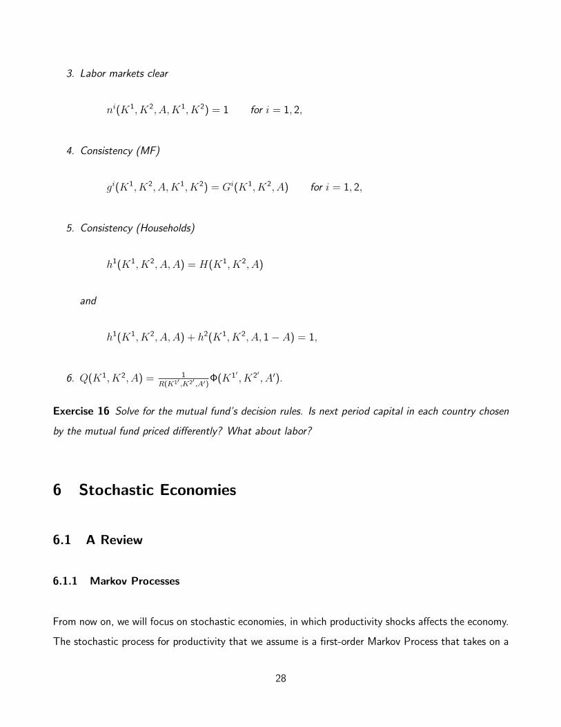
3. Labor markets clear
ni(K1, K2, A,K1, K2) = 1 for i = 1, 2,
4. Consistency (MF)
gi(K1, K2, A,K1, K2) = Gi(K1, K2, A) for i = 1, 2,
5. Consistency (Households)
h1(K1, K2, A,A) = H(K1, K2, A)
and
h1(K1, K2, A,A) + h2(K1, K2, A, 1− A) = 1,
6. Q(K1, K2, A) = 1R(K1′ ,K2′ ,A′)
Φ(K1′ , K2′ , A′).
Exercise 16 Solve for the mutual fund’s decision rules. Is next period capital in each country chosen
by the mutual fund priced differently? What about labor?
6 Stochastic Economies
6.1 A Review
6.1.1 Markov Processes
From now on, we will focus on stochastic economies, in which productivity shocks affects the economy.
The stochastic process for productivity that we assume is a first-order Markov Process that takes on a
28

finite number of values in the set Z = z1 < · · · < znz. A first order Markov process implies
Pr(zt+1 = zj|ht) = Γij, zt(ht) = zi
where ht is the history of previous shocks. Γ is a Markov chain with the property that the elements of
each rows sum to 1.
Let µ be a probability distribution over initial states, i.e.
∑i
µi = 1
and µi ≥ 0 ∀i = 1, ..., nz.
For next periods the probability distribution can be found by µ′ = ΓTµ.
If Γ is “nice” then ∃ a unique µ∗ s.t. µ∗ = ΓTµ∗ and µ∗ = limm→∞(ΓT )mµ0, ∀µ0 ∈ ∆i.
Γ induces the following probability distribution conditional on the initial draw z0 on ht = z0, z1, ..., zt:
Π(z0, z1) = Γi,. for z0 = zi.
Π(z0, z1, z2) = ΓTΓi,. for z0 = zi.
Then, Π(ht) is the probability of history ht conditional on z0. The expected value of z′ is∑
z′ Γzz′z′
and∑
z′ Γzz′ = 1.
6.1.2 Problem of the Social Planner
Let productivity affect the production function in a multiplicative fashion; i.e. technology is zF (K,N),
where z is a shock that follows a Markov chain on a finite state-space. Recall that the problem of the
29
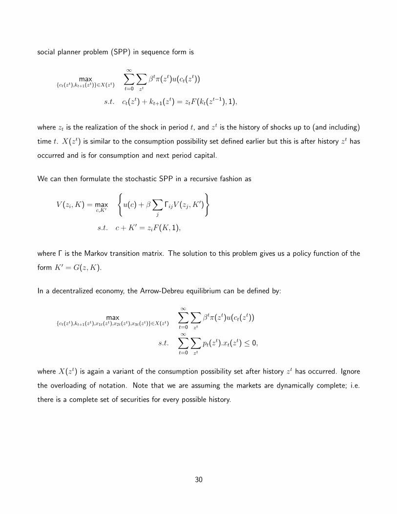
social planner problem (SPP) in sequence form is
maxct(zt),kt+1(zt)∈X(zt)
∞∑t=0
∑zt
βtπ(zt)u(ct(zt))
s.t. ct(zt) + kt+1(zt) = ztF (kt(z
t−1), 1),
where zt is the realization of the shock in period t, and zt is the history of shocks up to (and including)
time t. X(zt) is similar to the consumption possibility set defined earlier but this is after history zt has
occurred and is for consumption and next period capital.
We can then formulate the stochastic SPP in a recursive fashion as
V (zi, K) = maxc,K′
u(c) + β
∑j
ΓijV (zj, K′)
s.t. c + K ′ = ziF (K, 1),
where Γ is the Markov transition matrix. The solution to this problem gives us a policy function of the
form K ′ = G(z,K).
In a decentralized economy, the Arrow-Debreu equilibrium can be defined by:
maxct(zt),kt+1(zt),x1t(zt),x2t(zt),x3t(zt)∈X(zt)
∞∑t=0
∑zt
βtπ(zt)u(ct(zt))
s.t.∞∑t=0
∑zt
pt(zt).xt(z
t) ≤ 0,
where X(zt) is again a variant of the consumption possibility set after history zt has occurred. Ignore
the overloading of notation. Note that we are assuming the markets are dynamically complete; i.e.
there is a complete set of securities for every possible history.
30
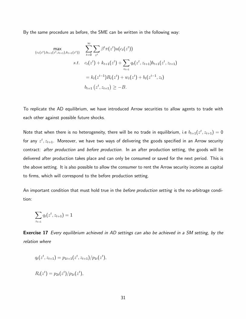
By the same procedure as before, the SME can be written in the following way:
maxct(zt),bt+1(zt,zt+1),kt+1(zt)
∞∑t=0
∑zt
βtπ(zt)u(ct(zt))
s.t. ct(zt) + kt+1(zt) +
∑zt+1
qt(zt, zt+1)bt+1(zt, zt+1)
= kt(zt−1)Rt(z
t) + wt(zt) + bt(z
t−1, zt)
bt+1
(zt, zt+1
)≥ −B.
To replicate the AD equilibrium, we have introduced Arrow securities to allow agents to trade with
each other against possible future shocks.
Note that when there is no heterogeneity, there will be no trade in equilibrium, i.e bt+1(zt, zt+1) = 0
for any zt, zt+1. Moreover, we have two ways of delivering the goods specified in an Arrow security
contract: after production and before production. In an after production setting, the goods will be
delivered after production takes place and can only be consumed or saved for the next period. This is
the above setting. It is also possible to allow the consumer to rent the Arrow security income as capital
to firms, which will correspond to the before production setting.
An important condition that must hold true in the before production setting is the no-arbitrage condi-
tion:
∑zt+1
qt(zt, zt+1) = 1
Exercise 17 Every equilibrium achieved in AD settings can also be achieved in a SM setting, by the
relation where
qt(zt, zt+1) = p1t+1(zt, zt+1)/p1t(z
t),
Rt(zt) = p2t(z
t)/p1t(zt),
31

and
wt(zt) = p3t(z
t)/p1t(zt).
Check from the FOC’s that the we get the same allocations in the two settings.
Exercise 18 The problem above assumes state contingent goods are delivered in terms of consumption
goods. Instead of this assume they are delivered in terms of capital goods. Show that the same
allocation would be achieved in both settings.
6.1.3 Recursive Competitive Equilibrium
Assume that households can trade state contingent assets, as in the sequential markets case above.
Then, we can write a household’s problem in recursive form as:
V (K, z, a) = maxc,k′,b(z′)
u (c) + β∑z′
Γzz′V (K ′, z′, a′ (z′))
s.t. c + k′ +∑z′
qz′ (K, z) b (z′) = w (K, z) + aR (K, z)
K ′ = G (K, z)
a′ (z′) = k′ + b (z′) .
Exercise 19 Write the FOC’s for this problem, given prices and the law of motion for aggregate capital.
Definition 9 A Recursive Competitive Equilibrium is a collection of functions V , k′, d, G, w, and R,
so that
1. Given G, w, and R, V solves the household’s functional equation, with k′ and b as the associated
policy function,
2. b (K, z,K; z′) = 0, for all z′,
32
3. k′ (K, z,K) = G (K, z),
4. w (K, z) = zFn (K, 1) and R (K, z) = zFk (K, 1),
5. and∑
z′ qz′ (K, z) = 1.
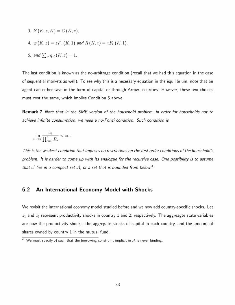
The last condition is known as the no-arbitrage condition (recall that we had this equation in the case
of sequential markets as well). To see why this is a necessary equation in the equilibrium, note that an
agent can either save in the form of capital or through Arrow securities. However, these two choices
must cost the same, which implies Condition 5 above.
Remark 7 Note that in the SME version of the household problem, in order for households not to
achieve infinite consumption, we need a no-Ponzi condition. Such condition is
limt→∞
at∏ts=0 Rs
<∞.
This is the weakest condition that imposes no restrictions on the first order conditions of the household’s
problem. It is harder to come up with its analogue for the recursive case. One possibility is to assume
that a′ lies in a compact set A, or a set that is bounded from below.4
6.2 An International Economy Model with Shocks
We revisit the international economy model studied before and we now add country-specific shocks. Let
z1 and z2 represent productivity shocks in country 1 and 2, respectively. The aggreagte state variables
are now the productivity shocks, the aggregate stocks of capital in each country, and the amount of
shares owned by country 1 in the mutual fund.
4 We must specify A such that the borrowing constraint implicit in A is never binding.
33

The problem of an household in country i is:
V i (z1, z2, K1, K2, A, a) = maxc,a′(~z′)
u (c) + β∑~z′
Γ~z~z′Vi(~z′, ~K ′, A′(~z′), a′(~z′)
)s.t. c +
∑~z′
q(~z, ~K,A, ~z′)a′(~z′) = wi (zi, Ki) + aΦ(~z, ~K,A)
K ′i = Gi
(~z, ~K,A
), for i = 1, 2
A(~z′) = H(~z, ~K,A, ~z′
)∀~z′
Let decision rule for next period asset holdings be a′(~z′) = h(~z, ~K,A, a, ~z′) ∀~z′. Note the financial
market structure assumed here. As before, labor is immobile and thus wages are country-specific and
given by wi(zi, Ki) = ziFN(Ki, 1).
Exercise 20 Write this economy with state-contingent claims in own country only.
Exercise 21 Write this economy where individuals can move freely in advance, but with incomplete
markets.
Now let’s look at the net present value of the mutual fund in equilibrium:
Φ(~z, ~K,A) =∑zi
[ziF (Ki, 1)− wi(zi, Ki)
]−∑i
Gi(~z, ~K,A) +∑~z′
Γ~z~z′Q(~z′, G(~z, ~K,A), H(~z, ~K,A, ~z′))Φ(~z′, G(~z, ~K,A), H(~z, ~K,A, ~z′)) (5)
where Q represents intertemporal prices, which in equilibrium should satisfy ∀~z′:
q(~z, ~K,A, ~z′) = Q(~z′, G(~z, ~K,A), H(~z, ~K,A, ~z′))Φ(~z′, G(~z, ~K,A), H(~z, ~K,A, ~z′))
Exercise 22 There is one more condition for Gi that equates expected return in each country. What
is it?
34

Definition 10 A Recursive Competitive Equilibrium for the (world’s) economy is a set of functions V i,
hi, wi, Gi for i ∈ 1, 2, and q, H, Q, and Φ such that the following conditions hold:
1. Given prices and laws of motion, V i and hi solve the household’s problem in country i for
i ∈ 1, 2,
2. The representative agent condition must hold:
h1(~z, ~K,A,A, ~z′
)= H
(~z, ~K,A,A, ~z′
)∀~z′,
3. The sum of shares in the mutual fund must be 1:
h1(~z, ~K,A,A, ~z′
)+ h2
(~z, ~K,A, 1− A, ~z′
)= 1 ∀~z′,
4. The mutual fund’s value Φ satisfies equation 5
5. wi(zi, Ki) is equated to the marginal products of labor in each country i for i ∈ 1, 2,
6. Expected rate of return on capital is the same across countries,
7. q(~z, ~K,A, ~z′) = Q(~z′, G(~z, ~K,A), H(~z, ~K,A, ~z′))Φ(~z′, G(~z, ~K,A), H(~z, ~K,A, ~z′)) ∀~z′,
8. The aggregate resource constraint must hold:
∑i
[ziF (Ki, 1)−Gi(~z, ~K,A)−
(wi (zi, Ki) + AiΦ(~z, ~K,A)−
∑~z′
q(~z, ~K,A, ~z′)hi(~z, ~K,A,Ai, ~z
′))]
= 0
where A1 = A and A2 = 1− A.
6.3 Heterogeneity in Wealth and Skills with Complete Markets
Now, let us consider a model in which we have two types of households, with equal measure µi = 1/2,
that care about leisure, but differ in the amount of wealth they own as well as their labor skill. There
35

is also uncertainty and Arrow securities like we have seen before.
Let A1 and A2 be the aggregate asset holdings of the two types of agents. These will now be state
variables for the same reason K1 and K2 were state variables earlier. The problem of an agent i ∈ 1, 2
with wealth a is given by
V i(z, A1, A2, a
)= max
c,n,a′(z′)u (c, n) + β
∑z′
Γzz′Vi(z′, A1′(z′), A2′(z′), a′(z′)
)s.t. c +
∑z′
q(z, A1, A2, z′
)a′ (z′) = R (z,K,N) a + W (z,K,N) εin
Ai′(z′) = Gi
(z, A1, A2, z′
), for i = 1, 2,∀z′
N = H(z, A1, A2
)K =
A1 + A2
2.
Let gi(z, A1, A2, ai) and hi(z, A1, A2, ai) be the asset and labor policy functions be the solution of each
type i to this problem. Then, we can define the RCE as below.
Definition 11 A Recursive Competitive Equilibrium with Complete Markets is a set of functions V i,
gi, hi, Gi for i ∈ 1, 2, R, w, H, and q, such that:
1. Given prices and laws of motion, V i, gi and hi solve the problem of household i for i ∈ 1, 2,
2. Labor markets clear:
H (z, A1, A2) = ε1h1 (z, A1, A2, A1) + ε2h
2 (z, A1, A2, A2),
3. The representative agent condition:
Gi (z, A1, A2, z′) = gi (z, A1, A2, Ai, z′) for i = 1, 2,∀z′
4. The average price of the Arrow security must satisfy:∑z′ q (z, A1, A2, z′) = 1,
5. G1 (z, A1, A2, z′) + G2 (z, A1, A2, z′) is independent of z′ (due to market clearing).
36
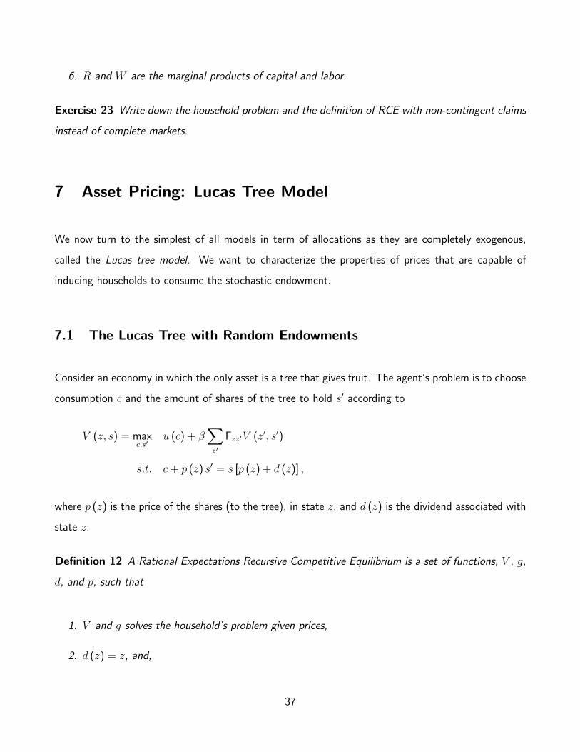
6. R and W are the marginal products of capital and labor.
Exercise 23 Write down the household problem and the definition of RCE with non-contingent claims
instead of complete markets.
7 Asset Pricing: Lucas Tree Model
We now turn to the simplest of all models in term of allocations as they are completely exogenous,
called the Lucas tree model. We want to characterize the properties of prices that are capable of
inducing households to consume the stochastic endowment.
7.1 The Lucas Tree with Random Endowments
Consider an economy in which the only asset is a tree that gives fruit. The agent’s problem is to choose
consumption c and the amount of shares of the tree to hold s′ according to
V (z, s) = maxc,s′
u (c) + β∑z′
Γzz′V (z′, s′)
s.t. c + p (z) s′ = s [p (z) + d (z)] ,
where p (z) is the price of the shares (to the tree), in state z, and d (z) is the dividend associated with
state z.
Definition 12 A Rational Expectations Recursive Competitive Equilibrium is a set of functions, V , g,
d, and p, such that
1. V and g solves the household’s problem given prices,
2. d (z) = z, and,
37

3. g(z, 1) = 1, for all z.
To explore the problem further, note that the FOC for the household’s problem imply the equilibrium
condition
uc (c (z, 1)) = β∑z′
Γzz′
[p (z′) + d (z′)
p (z)
]uc (c (z′, 1)) .
where we have uc (z) := uc (c (z, 1)). Then this simplifies to
p (z)uc (z) = β∑z′
Γzz′uc (z′) [p (z′) + z′] ∀z.
Exercise 24 Derive the Euler equation for household’s problem to show the result above.
Note that this is just a system of nz equations with unknowns p (zi)ni=1. We can use the power of
matrix algebra to solve the system. To do so, let:
p :=
p (z1)
...
p (zn)
(nz×1)
,
and
uc :=
uc (z1) 0
. . .
0 uc (zn)
(nz×nz)
.
Then
uc.p =
p (z1)uc (z1)
...
p (zn)uc (zn)
(nz×1)
,
38

and
uc.z =
z1uc (z1)
...
znuc (zn)
(nz×1)
,
Now, rewrite the system above as
ucp = βΓucz + βΓucp,
where Γ is the transition matrix for z, as before. Hence, the price for the shares is given by
(Inz − βΓ) ucp = βΓucz,
or
p = ([Inz − βΓ] uc)−1 βΓucz,
where p is the vector of prices that clears the market.
Exercise 25 How are prices defined when the agent faces taste shocks?
7.2 Asset Pricing
Consider our simple model of Lucas tree with fluctuating output. What is the definition of an asset in
this economy? It is “a claim to a chunk of fruit, sometime in the future.”
If an asset, a, promises an amount of fruit equal to at (zt) after history zt = (z0, z1, . . . , zt) of shocks,
after a set of (possible) histories in H, the price of such an entitlement in date t = 0 is given by:
p (a) =∑t
∑zt∈H
q0t
(zt)at(zt),
39

where q0t (zt) is the price of one unit of fruit after history zt in today’s “dollars”; this follows from a
no-arbitrage argument. If we have the date t = 0 prices, qt, as functions of histories, we can replicate
any possible asset by a set of state-contingent claims and use this formula to price that asset.
To see how we can find prices at date t = 0, consider a world in which the agent wants to solve
maxct(zt)
∞∑t=0
βt∑zt
πt(zt)u(ct(zt))
s.t.∞∑t=0
∑zt
q0t
(zt)ct(zt)≤
∞∑t=0
∑ht
q0t
(zt)zt.
This is the familiar Arrow-Debreu market structure, where the household owns a tree, and the tree
yields z ∈ Z amount of fruit in each period. The FOC for this problem imply:
q0t
(zt)
= βtπt(zt) uc (zt)
uc (z0).
This enables us to price the good in each history of the world and price any asset accordingly.
Comment 1 What happens if we add state-contingent shares b into our recursive model? Then the
agent’s problem becomes:
V (z, s, b) = maxc,s′,b′(z′)
u (c) + β∑z′
Γzz′V (z′, s′, b′ (z′))
s.t. c + p (z) s′ +∑z′
q (z, z′) b′ (z′) = s [p (z) + z] + b.
A characterization of q can be obtained by the FOC, evaluated at the equilibrium, and thus written as:
q (z, z′)uc (z) = βΓzz′uc (z′) .
We can thus price all types of securities using p and q in this economy.
To see how we can price an asset given today’s shock is z, consider the option to sell it tomorrow at
40

price P as an example. The price of such an asset today is
q (z, P ) =∑z′
q (z, z′) max P − p (z′) , 0 ,
where the agent has the option not to sell it. The American option to sell at price P either tomorrow
or the day after tomorrow is priced as:
q (z, P ) =∑z′
q (z, z′) max P − p (z′) , q (z′, P ) .
Similarly, an European option to buy the asset at price P the day after tomorrow is priced as:
q (z, P ) =∑z′
∑z′′
max p (z′′)− P, 0 q (z′, z′′) q (z, z′) .
Note that R (z) = [∑
z′ q (z, z′)]−1 is the gross risk free rate, given today’s shock is z. The unconditional
gross risk free rate is then given by Rf =∑
z µ∗zR(z) where µ∗ is the steady-state distribution of the
shocks.
The average gross rate of return on the stock market is∑
z µ∗z
∑z′ Γzz′
[p(z′)+z′
p(z)
]and the risk pre-
mium is the difference between this rate and the unconditional gross risk free rate (i.e. given by∑z µ∗z
(∑z′ Γzz′
[p(z′)+z′
p(z)
]−R(z)
)).
Exercise 26 Use the expressions for p and q and the properties of the utility function to show that
risk premium is positive.
7.3 Taste Shocks
Consider an economy in which the only asset is a tree that gives fruits. The fruit is constant over
time (normalized to 1) but the agent is subject to preference shocks for the fruit each period given by
41

θ ∈ Θ. The agent’s problem in this economy is
V (θ, s) = maxc,s′
θu (c) + β∑θ′
Γθθ′V (θ′, s′)
s.t. c + p (θ) s′ = s [p (θ) + d (θ)] .
The equilibrium is defined as before. The only difference is that, now, we must have d (θ) = 1 since
z is normalized to 1. What does it mean that the output of the economy is constant (fixed at one),
but the tastes for this output change? In this setting, the function of the price is to convince agents to
keep their consumption constant even in the presence of taste shocks. All the analysis follows through
as before once we write the FOC’s characterizing the prices of shares, p (θ), and state-contingent prices
q (θ, θ′).
This is a simple model, in the sense that the household does not have a real choice regarding con-
sumption and savings. Due to market clearing, household consumes what nature provides her. In each
period, according to the state of productivity z and taste θ, prices adjusts such that household would
like to consume z, which is the amount of fruit that the nature provides. In this setup, output is equal
to z. If we look at the business cycle in this economy, the only source of output fluctuations is caused
by nature. Eveyrhing determined by the supply side of the economy and the demand side has indeed
no impact on output.
In next section, we are going to introduce search frictions to incorporate a role for the demand side
into our model.
8 Endogenous Productivity in a Product Search Model
We will model the situation in which households need to find the fruit before consuming it.5 Assume
that households have to find the tree in order to consume the fruit. Finding trees is characterized by
5 Think of fields in The Land of Apples, full of apples, that ,are owned by firms; agents have to buy the apples. Inaddition, they have to search for them as well!
42

a constant returns to scale (increasing in both arguments) matching function M (T,D),6 where T is
the number of trees in the economy and D is the aggregate shopping effort exerted by households
when searching. The probability that a tree finds a shopper is given by M(T,D)T
, i.e. the total number
of matches divided by the number of trees. The probability that a unit of shopping effort finds a tree
is given by M(T,D)D
, i.e. the total number of matches divided by the economy’s effort level.
Let’s assume that M(T,D) takes the form DϕT 1−ϕ and denote 1Q
:= DT
, i.e. the ratio of shoppers per
trees, as capturing the market tightness (and thus Q = TD
). The probability of a household finding a
tree is given by Ψh (Q) := M(T,D)D
= Q1−ϕ and thus the higher the number of people searching, the
smaller the probability of a household finding a tree. The probability of a tree finding a household is
then given by Ψf (Q) := M(T,D)T
= Q−ϕ, and thus the higher the number of people searching, the
higher the probability of a tree finding a shopper. Note that in this economy the number of trees is
constant and equal to one.7
Let us assume households face a demand side shock θ and a supply side shock z. They are follow
independent Markov processes with transitional probabilities Γθθ′ and Γzz′ , respectively. Households
choose the consumption level c, the search effort exerted to get the fruit d, and the shares of the tree
to hold next period s′. The household’s problem can be written as
V (θ, z, s) = maxc,d,s′
u (c, d, θ) + β∑θ′,z′
Γθθ′Γzz′V (θ′, z′, s′) (6)
s.t. c + P (θ, z) s′ = P (θ, z)[s(
1 + R (θ, z))]
(7)
c = d Ψh (Q (θ, z)) z. (8)
6 What does the fact that M is constant returns to scale imply?7 It is easy to find the statements for Ψh and Ψf , given the Cobb-Douglas matching function:
Ψh (Q) =DϕT 1−ϕ
D=
(T
D
)1−ϕ
= Q1−ϕ,
Ψf (Q) =DϕT 1−ϕ
T=
(T
D
)−ϕ= Q−ϕ.
The question is: is Cobb-Douglas an appropriate choice for the matching function, or its choice is a matter ofsimplicity?
43

where P is the price of the tree relative to that of consumption and R is the dividend income (in units
of the tree). Note that the equation 7 is our standard budget constraint, while equation 8 corresponds
to the shopping constraint.
Note some notation conventions here. P (θ, z) is in terms of consumption goods, while R(θ, z) is in
terms of shares of the tree (that’s why we are using the hat). We could also write the household
budget constraint in terms of the price of consumption relative to that of the tree. To do so, let’s
define P (θ, z) = 1P (θ,z)
as the price of consumption goods in terms of the tree. Then the budget
constraint can be defined as:
cP (θ, z) + s′ = s(
1 + R (θ, z))
Let’s maintain our notation with P (θ, z) and R(θ, z) from now on. We can substitute the constraints
into the objective and solve for d in order to get the Euler equation for the household. Using the market
clearing condition in equilibrium, the problem reduces to one equation and two unknowns, P (θ, z) and
Q(θ, z) (other objects, C,D and R are known functions of P and Q, and the amount shares of the tree
in equilibrium is 1 as before). We thus still need another functional equation to sovel for the equilibrium
of this economy, i.e. we need to specify the search protocol. We now turn to one way of doing so.
Exercise 27 Derive the Euler equation of the household from the problem defined above.
8.1 Competitive Search
Competitive search is a particular search protocol of what is called non-random (or directed) search.
To understand this protocol, consider a world consisting of a large number of islands. Each island has
a sign that displays two numbers, P (θ, z) and Q(θ, z). P (θ, z) is the price on the island and Q(θ, z)
is a measure of market tightness in that island (or if the price is a wage rate W , then Q is the number
of workers on the island divided by the number of job opportunities in that island). Both individuals
and firms have to decide to go to one island. For instance, in an island with a higher wage, the worker
44

might have a higher income conditional on finding a job. However, the probability of finding a job
might be low on that island given the tightness of the labor market on that island. The same story
holds for the job owners, who are searching to hire workers.
In our economy, both firms and workers search for specific markets indexed by price P and a market
tightness Q.8 An island, or a pair of (P,Q), is operational if there exists some consumer and firm
choosing that market. Therefore, an agent should choose P and Q such that it gives sufficient profit
to the firm, so that it wants to be in that island as opposed to doing something else, which will be
determined in the equilibrium. Competitive search is magic in the sense that it does not presuppose a
particular pricing protocol that other search protocols need (e.g. bargaining).
Maintaining the demand shock θ and supply side shock z we introduced before, we can then define the
household problem with competitive search as follows
V (θ, z, s) = maxc,d,s′,P,Q
u (c, d, θ) + β∑θ′,z′
Γθθ′Γzz′V (θ′, z′, s′) (9)
s.t. c + Ps′ = P[s(
1 + R (θ, z))], (10)
c = d Ψh (Q) z (11)
zΨf (Q)
P≥ R(θ, z) (12)
Let u (c, d, θ) = u (θc, d) from here on. The first two constraints were defined above, while the last
is the firm’s participation constraint, which is the condition that states that firms would prefer this
market to other markets in which they would get R(θ, z).
To solve the problem, let’s take the first order conditions. One way to do this is to first plug the first
two constraints into the objective function (expressing c and s′ as functions of d) and then take the
8 From now on, we will drop the arguments of P and Q.
45

derivative with respect to d (recall that Ψh = Q1−ϕ) to get:
θQ1−ϕzuc(θdQ1−ϕz, d) + ud(θdQ1−ϕz, d) =
β∑θ′,z′
Γθθ′Γzz′V3
(θ′, z′, s(1 + R(θ, z))− dQ1−ϕz
P
)Q1−ϕz
P(13)
To find V3 consider the original problem where constraints are not plugged into the objective function.
Using the envelope theorem we get:
V3(θ, z, s) =
[θuc(θdQ
1−ϕz, d) +ud(θdQ1−ϕz, d)
Q1−ϕz
]P (1 + R(θ, z))
Combining these two gives the Euler equation:
θuc(θdQ1−ϕz, d) +
ud(θdQ1−ϕz, d)
Q1−ϕz=
β∑θ′,z′
Γθθ′Γzz′P ′(1 + R(θ′, z′))
P
[θ′uc(θ
′d′Q′1−ϕ
z′, d′) +ud(θ′d′Q′1−ϕz′, d′)
Q′1−ϕz′
](14)
Observe that this equation is the same as the Euler equation from the random search model. This
gives us the optimal search and saving behavior for a given island (i.e. a market tightness 1/Q and
price level P ). To understand which market to search in, we need to look at the FOC with respect to
Q and P . Let λ denote the Lagrange multiplier on the firm’s participation constraint, then the FOC
with respect to Q and P are respectively:
θd(1− ϕ)Q−ϕzuc(θdQ1−ϕz, d) =
β∑θ′,z′
Γθθ′Γzz′V3
(θ′, z′, s(1 + R(θ, z))− dQ1−ϕz
P
)d(1− ϕ)Q−ϕz
P− λϕQ
−ϕ−1z
P(15)
46
and
β∑θ′,z′
Γθθ′Γzz′V3
(θ′, z′, s(1 + R(θ, z))− dQ1−ϕz
P
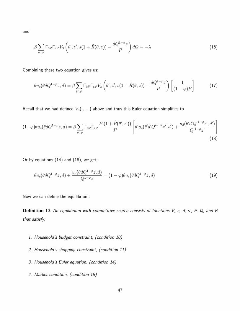
)dQ = −λ (16)
Combining these two equation gives us:
θuc(θdQ1−ϕz, d) = β
∑θ′,z′
Γθθ′Γzz′V3
(θ′, z′, s(1 + R(θ, z))− dQ1−ϕz
P
)[1
(1− ϕ)P
](17)
Recall that we had defined V3(·, ·, ·) above and thus this Euler equation simplifies to
(1−ϕ)θuc(θdQ1−ϕz, d) = β
∑θ′,z′
Γθθ′Γzz′P ′(1 + R(θ′, z′))
P
[θ′uc(θ
′d′Q′1−ϕ
z′, d′) +ud(θ′d′Q′1−ϕz′, d′)
Q′1−ϕz′
](18)
Or by equations (14) and (18), we get:
θuc(θdQ1−ϕz, d) +
ud(θdQ1−ϕz, d)
Q1−ϕz= (1− ϕ)θuc(θdQ
1−ϕz, d) (19)
Now we can define the equilibrium:
Definition 13 An equilibrium with competitive search consists of functions V, c, d, s’, P, Q, and R
that satisfy:
1. Household’s budget constraint, (condition 10)
2. Household’s shopping constraint, (condition 11)
3. Household’s Euler equation, (condition 14)
4. Market condition, (condition 18)
47
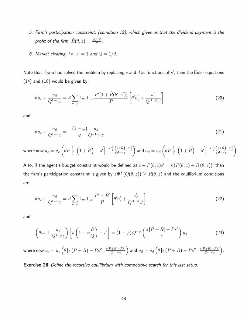
5. Firm’s participation constraint, (condition 12), which gives us that the dividend payment is the
profit of the firm, R(θ, z) = zQ−ϕ
P,
6. Market clearing, i.e. s′ = 1 and Q = 1/d.
Note that if you had solved the problem by replacing c and d as functions of s′, then the Euler equations
(14) and (18) would be given by:
θuc +ud
Q1−ϕz= β
∑θ′,z′
Γθθ′Γzz′P ′(1 + R(θ′, z′))
P
[θ′u′c +
u′dQ′1−ϕz′
](20)
and
θuc +ud
Q1−ϕz= −(1− ϕ)
ϕ
udQ−1−ϕz
(21)
where now uc = uc
(θP[s(
1 + R)− s′
],P [s(1+R)−s′]
Q1−ϕz
)and ud = ud
(θP[s(
1 + R)− s′
],P [s(1+R)−s′]
Q1−ϕz
).
Also, if the agent’s budget constraint would be defined as c + P (θ, z)s′ = s (P (θ, z) + R (θ, z)), then
the firm’s participation constraint is given by zΨf (Q(θ, z)) ≥ R(θ, z) and the equilibrium conditions
are
θuc +ud
Q1−ϕz= β
∑θ′,z′
Γθθ′Γzz′P ′ + R′
P
[θ′u′c +
u′dQ′1−ϕz′
](22)
and
(θuc +
udQ1−ϕz
)[s
(1− ϕR
Q
)− s′
]= (1− ϕ)Q−ϕ
(s [P + R]− Ps′
z
)ud (23)
where now uc = uc
(θ [s (P + R)− Ps′] , s[P+R]−Ps′
Q1−ϕz
)and ud = ud
(θ [s (P + R)− Ps′] , s[P+R]−Ps′
Q1−ϕz
).
Exercise 28 Define the recursive equilibrium with competitive search for this last setup.
48
8.1.1 Firms’ Problem
Note that in any given period a firm maximizes its returns to the tree by choosing the appropriate
market, Q. Note that, by choosing a market Q, the firm is effectively choosing a price. Let the
numeraire be the price of trees, then P (Q) is price of consumption.
Since there is nothing dynamic in the choice of a market (note that, we are assuming firms can choose
a different market in each period), we can write the problem of a firm as:
π = maxQ
P (Q) Ψf (Q) z. (24)
The first order condition for the optimal choice of Q is
P ′ (Q) Ψf (Q) + P (Q) Ψf ′ (Q) = 0, (25)
which then determines P (Q) as
P ′ (Q)
P (Q)= −Ψf ′ (Q)
Ψf (Q). (26)
9 Measure Theory
This section will be a quick review of measure theory, so that we are able to use it in the subsequent
sections. In macroeconomics we encounter the problem of aggregation often and it’s crucial that we
do it in a reasonable way. Measure theory is a tool that tells us when and how we could do so. Let us
start with some definitions on sets.
Definition 14 For a set S, S is a family of subsets of S, if B ∈ S implies B ⊆ S (but not the other
way around).
49

Remark 8 Note that in this section we will assume the following convention
1. small letters (e.g. s) are for elements,
2. capital letters (e.g. S) are for sets, and
3. fancy letters (e.g. S) are for a set of subsets (or families of subsets).
Definition 15 A family of subsets of S, S, is called a σ-algebra in S if
1. S, ∅ ∈ S;
2. if A ∈ S ⇒ Ac ∈ S (i.e. S is closed with respect to complements and Ac = S\A); and,
3. for Bii∈N, if Bi ∈ S for all i ⇒⋂i∈NBi ∈ S (i.e. S is closed with respect to countable
intersections and by De Morgan’s laws, S is closed under countable unions).
Example 1
1. The power set of S (i.e. all the possible subsets of a set S), is a σ-algebra in S.
2. ∅, S is a σ-algebra in S.
3.∅, S, S1/2, S2/2
, where S1/2 means the lower half of S (imagine S as an closed interval in R),
is a σ-algebra in S.
4. If S = [0, 1], then
S =
∅,[
0,1
2
),
1
2
,
[1
2, 1
], S
is not a σ-algebra in S. But
S =
∅,
1
2
,
[0,
1
2
)∪(
1
2, 1
], S
is a σ-algebra in S.
50

Why do we need the σ-algebra? Because it defines which sets may be considered as “events”: things
that have positive probability of happening. Elements not in it may have no properly defined measure.
Basically, a σ-algebra is the ”patch” that lets us avoid some pathological behaviors of mathematics,
namely non-measurable sets. We are now ready to define a measure.
Definition 16 Suppose S is a σ-algebra in S. A measure is a real-valued function x : S → R+, that
satisfies
1. x (∅) = 0;
2. if B1, B2 ∈ S and B1 ∩B2 = ∅ ⇒ x (B1 ∪B2) = x (B1) + x (B2) (additivity); and,
3. if Bii∈N ∈ S and Bi ∩Bj = ∅ for all i 6= j ⇒ x (∪iBi) =∑
i x (Bi) (countable additivity).9
Put simply, a measure is just a way to assign each possible “event” a non-negative real number. A set
S, a σ-algebra in it (S), and a measure on S (x) define a measurable space, (S,S, x).
Definition 17 A Borel σ-algebra is a σ-algebra generated by the family of all open sets B (generated
by a topology). A Borel set is any set in B.
Since a Borel σ-algebra contains all the subsets generated by the intervals, you can recognize any subset
of a set using a Borel σ-algebra. In other words, a Borel σ-algebra corresponds to complete information.
Definition 18 A probability measure is a measure with the property that x (S) = 1 and thus (S,S, x)
is now a probability space. The probability of an event is then given by x(A), where A ∈ S.
Definition 19 Given a measurable space (S,S, x), a real-valued function f : S → R is measurable
(with respect to the measurable space) if, for all a ∈ R, we have
b ∈ S | f(b) ≤ a ∈ S.9 Countable additivity means that the measure of the union of countable disjoint sets is the sum of the measure of these
sets.
51
Given two measurable spaces (S,S, x) and (T, T , z), a function f : S → T is measurable if for all
A ∈ T , we have
b ∈ S | f(b) ∈ A ∈ S.
One way to interpret a σ-algebra is that it describes the information available based on observations,
i.e. a structure to organize information. Suppose that S is comprised of possible outcomes of a dice
throw. If you have no information regarding the outcome of the dice, the only possible sets in your
σ-algebra can be ∅ and S. If you know that the number is even, then the smallest σ-algebra given that
information is S = ∅, 2, 4, 6 , 1, 3, 5 , S. Measurability has a similar interpretation. A function is
measurable with respect to a σ-algebra S, if it can be evaluated under the current measurable space
(S,S, x).
Example 2 Suppose S = 1, 2, 3, 4, 5, 6. Consider a function f that maps the element 6 to the
number 1 (i.e. f(6) = 1) and any other elements to -100. Then f is NOT measurable with respect to
S = ∅, 1, 2, 3, 4, 5, 6, S. Why? Consider a = 0, then b ∈ S | f(b) ≤ a = 1, 2, 3, 4, 5. But
this set is not in S.
We can also generalize Markov transition matrices to any measurable space, which is what we do next.
Definition 20 Given a measurable space (S,S, x), a function Q : S × S → [0, 1] is a transition
probability if
1. Q (s, ·) is a probability measure for all s ∈ S; and,
2. Q (·, B) is a measurable function for all B ∈ S.
Intuitively, for B ∈ S and s ∈ S, Q (s, B) gives the probability of being in set B tomorrow, given that
52

the state is s today. Consider the following example: a Markov chain with transition matrix given by
Γ =
0.2 0.2 0.6
0.1 0.1 0.8
0.3 0.5 0.2
,
on the set S = 1, 2, 3, with the σ-algebra S = P (S) (where P (S) is the power set of S). If Γij
denotes the probability of state j happening, given the current state i, then
Q (3, 1, 2) = Γ31 + Γ32 = 0.3 + 0.5 .
As another example, suppose we are given a measure x on S with xi being the fraction of type i, for
any i ∈ S. Given the previous transition function, we can calculate the fraction of types that will be in
i tomorrow using the following formulas:
x′1 = x1Γ11 + x2Γ21 + x3Γ31,
x′2 = x1Γ12 + x2Γ22 + x3Γ32,
x′3 = x1Γ13 + x2Γ23 + x3Γ33.
In other words
x′ = ΓTx,
where xT = (x1, x2, x3).
To extend this idea to a general case with a general transition function, we define an updating operator
as T (x,Q), which is a measure on S with respect to the σ-algebra S, such that
x′ (B) =T (x,Q) (B)
=
∫S
Q (s, B)x (ds) , ∀B ∈ S,
53

where we integrated over all the possible current states s to get the probability of landing in set B
tomorrow.
A stationary distribution is a fixed point of T , that is x∗ such that
x∗ (B) = T (x∗, Q) (B) , ∀B ∈ S.
We know that, if Q has nice properties (monotone, Feller property, and enough mixing),10 then a unique
stationary distribution exists (for instance, we discard alternating from one state to another) and we
have that
x∗ = limn→∞
T n (x0, Q) ,
for any x0 in the space of probability measures on (S,S).
Exercise 29 Consider unemployment in a very simple economy (in which the transition matrix is
exogenous). There are two states of the world: being employed and being unemployed. The transition
matrix is given by
Γ =
0.95 0.05
0.50 0.50
.
Compute the stationary distribution corresponding to this Markov transition matrix.
10 See Chapters 11/12 in Stockey, Lucas, and Prescott (1989) for more details.
54
10 Industry Equilibrium
10.1 Preliminaries
Now we are going to study a type of models initiated by Hopenhayn. We will abandon the general
equilibrium framework from the previous sections to study the dynamics of the distribution of firms in
a partial equilibrium environment.
To motivate things, let’s start with the problem of a single firm that produces a good using labor as
input according to a technology described by the production function f(n). Let us assume that this
function is increasing, strictly concave, with f (0) = 0. A firm that hires n units of labor is able to
produce sf (n), where s is productivity. Markets are competitive, so a firm takes prices (p and w) as
given. A firm then chooses n in order to solve
π (s, p) = maxn≥0psf (n)− wn . (27)
The first order condition implies that in the optimum n∗ solves
psfn (n∗) = w. (28)
Let us denote the solution to this problem as the function n∗ (s, p).11 Given the above assumptions,
n∗ is an increasing function of both s (i.e. more productive firms have more workers) and p (i.e. the
higher the output price, the more workers will hire).
Suppose now there is a mass of firms in the industry, each associated with a productivity parameter
s ∈ S ⊂ R+, where S := [s, s]. Let S denote a σ-algebra on S (a Borel σ-algebra, for instance). Let x
be a probability measure defined over the space (S,S), which describes the cross-sectional distribution
of productivity among firms. Then, for any B ⊂ S with B ∈ S, x (B) is the mass of firms having
productivities in S.
11 As we declared in advance, this is a partial equilibrium analysis. Hence, we ignore the dependence of the solution onw to focus on the determination of p.
55

We will use x to define statistics of the industry. For example, at this point, it is convenient to define
the aggregate supply of the industry. Since individual supply is just sf (n∗ (s, p)), then the aggregate
supply can be written as12
Y S (p) =
∫S
sf (n∗ (s, p))x (ds) . (29)
Observe that Y S is a function of the price p only. For any price p, Y S (p) gives us the supply in this
economy.
Exercise 30 Search Wikipedia for an index of concentration in an industry and adopt it for our econ-
omy.
Suppose now that the demand of the market is described by some function Y D (p). Then the industry’s
equilibrium price p∗ is determined by the market clearing condition
Y D (p∗) = Y S (p∗) . (30)
So far, everything is too simple to be interesting. The ultimate goal here is to understand how the
object x is determined by the fundamentals of the industry. Hence, we will be adding tweaks to this
basic environment in order to obtain a theory of firms’ distribution in a competitive environment. Let’s
start by allowing firms to die.
10.2 A Simple Dynamic Environment
Consider now a dynamic environment, in which firms face the problem above every period. Firms
discount profits at rate rt, which is exogenously given. In addition, assume that a single firm faces a
probability 1− δ of disappearing in each period. In what follows, we will focus on stationary equilibria;
i.e. equilibria in which the price of the final output p, the rate of return, r, and the productivity of
12 S in Y S stands for supply.
56

firm, s, stay constant through time.
Notice first that the firm’s decision problem is still a static problem. We can easily write the value of
an incumbent firm with productivity s as
V (s; p) =∞∑t=0
(δ
1 + r
)tπ (s, p)
=
(1 + r
1 + r − δ
)π (s, p)
Note that we are considering that p is fixed (that is why we use a semicolon and therefore we can omit
it from the expressions above). Note also that every period there is positive mass of firms that die.
Then, how can this economy be in a stationary equilibrium? To achieve that, we have to assume that
there is a constant flow of firms entering the economy in each period as well, so that the mass of firms
that disappear is exactly replaced by new entering firms.
As before, let x be the measure describing the distribution of firms within the industry. The mass of
firms that die is given by (1− δ)x (S). We will allow these firms to be replaced by new entrants. These
entrants draw a productivity parameter s from a probability measure γ over (S,S).
One might ask what keeps these firms out of the market in the first place? If π (s; p) = psf (n∗ (s; p))−
wn∗ (s; p) > 0, which is the case for the firms operating in the market (since n∗ > 0), then all the
(potential entering) firms with productivities in S would want to enter the market.
We can fix this flaw by assuming that there is a fixed entry cost that each firm must pay in order to
operate in the market, denoted by cE. Moreover, we will assume that the entrant has to pay this cost
before learning s. Hence the value of a new entrant is given by the following function
V E (p) =
∫S
V (s; p) γ (ds)− cE. (31)
Entrants will continue to enter if V E is greater than 0 and decide not to enter if this value is less than
zero (since the option value from staying out of the market is 0). As a result, stationarity occurs when
57

V E is exactly equal to zero (this is the free-entry condition).13
Let’s analyze how this environment shapes the distribution of firms in the market. Let xt be the cross-
sectional distribution of firms in any given period t. For any B ⊂ S, a fraction 1 − δ of firms with
productivity s ∈ B will die and newcomers will enter the market (the mass of which is m). Hence, next
period’s measure of firms on set B will be given by
xt+1 (B) = δxt (B) + mγ (B) , . (32)
That is, the mass m of firms would enter the market in t + 1, but only fraction γ (B) of them will
have productivities in the set B. As you might suspect, this relationship must hold for every B ∈ S.
Moreover, since we are interested in stationary equilibria, the previous expression tells us that the
cross-sectional distribution of firms will be completely determined by γ.
If we let mapping T be defined as
Tx (B) = δx (B) + mγ (B) , ∀B ∈ S, (33)
a stationary distribution of productivity is the fixed point of the mapping T , i.e. x∗ such that Tx∗ = x∗,
which implies the following
x∗ (B;m) =m
1− δγ (B) , ∀B ∈ S. (34)
Now, note that the demand and supply condition in equation (30) takes the form
Y D (p∗ (m)) =
∫S
sf (n∗ (s; p)) dx∗ (s;m) , (35)
whose solution p∗ (m) is a continuous function under regularity conditions stated in Stockey, Lucas,
and Prescott (1989).
13 We are assuming that there is an infinite number (mass) of prospective firms willing to enter the industry.
58

We have two equations, (31) and (35), and two unknowns, p and m. Thus, we can defined the
equilibrium as follows
Definition 21 A stationary distribution for this environment consists of functions V , π∗, n∗, p∗, x∗,
and m∗, that satisfy:
1. Given prices, V , π∗, and n∗ solve the incumbent firm’s problem;
2. Y D (p∗ (m)) =∫Ssf (n∗ (s; p)) dx∗ (s;m);
3.∫sV (s; p) γ (ds)− cE = 0; and,
4. x∗ (B) = δx∗ (B) + m∗γ (B) , ∀B ∈ S.
10.3 Introducing Exit Decisions
We want to introduce more (economic) content by making the exit of firms endogenous (i.e. a decision
of the firm). One way to do so is to assume that the productivity of firms follows a Markov process
governed by the transition function Γ. This would change the mapping T in Equation (33) as
Tx (B) = δ
∫S
Γ (s, B)x (ds) + mγ (B) , ∀B ∈ S. (36)
But, this wouldn’t add much economic content to our environment; firms still do not make any (inter-
esting) decision. To change this, let’s introduce operating costs in the model. Suppose firms have to
pay cv each period in order to stay in the market. In this case, when s is low, the firm’s profit might
not cover its operating cost. The firm might therefore decide to leave the market. Note, however,
that the firm has already paid (the sunk cost of) cE from entering the market and since s follows a
first-order Markov process, the prospects of future profits might deter the firm from exiting the market.
Therefore, having negative profits in one period does not imply that the firm’s optimal choice is to
leave the market.
59
By adding such a minor change, the solution will have a reservation productivity property under some
conditions (to be discussed in the comment below). In words, there will be a minimum productivity,
s∗ ∈ S, above which it is profitable for the firm to stay in the market (and below which the firm decides
to exit).
To see this, note that the value of a firm currently operating in the market with productivity s ∈ S is
given by
V (s; p) = max
0, π (s; p) +
1
(1 + r)
∫S
V (s′; p) Γ (s, ds′)− cv. (37)
Exercise 31 Show that the firm’s decision takes the form of a reservation productivity strategy, in
which, for some s∗ ∈ S, s < s∗ implies that the firm would leave the market.
In this case, the law of motion of the distribution of productivities on S is given by
x′ (B) =
∫ s
s∗Γ (s, B ∩ [s∗, s])x (ds) + mγ (B ∩ [s∗, s]) , ∀B ∈ S. (38)
A stationary distribution of the firms in this economy, x∗, is the fixed point of this equation.
Example 3 How productive does a firm have to be, to be in the top 10% largest firms in this economy
(in the stationary equilibrium)? The answer to this question is the solution to the following equation
∫ ssx∗ (ds)∫ s
s∗x∗ (ds)
= 0.1,
where s is the productivity level above which a firm is in the top 10% largest firm. Then, the fraction
of the labor force in the top 10% largest firms in this economy, is
∫ ssn∗ (s, p)x∗ (ds)∫ s
s∗n∗ (s, p)x∗ (ds)
.
Exercise 32 Compute the average growth rate of the smallest one third of the firms. What would be
the fraction of firms in the top 10% largest firms in the economy that remain in the top 10% in next
60
period? What is the fraction of firms younger than five uears?
Comment 2 To see that that the firm’s decision is determined by a reservation productivity, we need
to start by showing that the profit function (before the variable cost) π (s; p) is increasing in s. Hence
the productivity threshold is given by the s∗ that satisfies the following condition:
π (s∗; p) = cv
for an equilibrium price p. Now instead of considering γ as the probability measure describing the
distribution of productivities among entrants, we consider γ defined as follows
γ (B) =γ (B ∩ [s∗, s])
γ ([s∗, s])
for any B ∈ S.
To make things more concrete and easier to compute, we will assume that s follows a Markov process.
To facilitate the exposition, let’s make S finite and assume s has the transition matrix Γ. Assume
further that Γ is regular enough so that it has a stationary distribution γ∗. For the moment we will not
put any additional structure on Γ.
The operating cost cv is such that the exit decision is meaningful since firms can have negative profits
in any given period and thus it is costly to keep doors open. Let’s analyze the problem from the
perspective of the firm’s manager. He has now two things to decide. First, he asks himself the question
“Should I stay or should I go?”. Second, conditional on staying, he has to decide how much labor to
hire. Importantly, notice that this second decision is still a static decision since the manager chooses
labor that maximizes the firm’s period profits. Later, we will introduce adjustment costs that will make
this decision a dynamic one.
Let Φ (s; p) be the value of the firm before having decided whether to stay in the market or to go. Let
61
V (s; p) be the value of the firm that has already decided to stay. Assuming w = 1, V (s; p) satisfies
V (s; p) = maxn
spf (n)− n− cv +
1
1 + r
∫s′∈S
Φ (s′; p) Γ(s, ds′)
(39)
Each morning the firm chooses d in order to solve
Φ (s; p) = maxd∈0,1
d V (s; p) (40)
Let d∗ (s; p) be the optimal decision to this problem. Then d∗ (s; p) = 1 means that the firm stays in
the market. One can alternatively write:
Φ (s; p) = maxd∈0,1
d
[π (s; p)− cv +
1
1 + r
∫s′∈S
Φ (s′; p) Γ(s, ds′)
](41)
or else
Φ (s; p) = max
π (s; p)− cv +
1
1 + r
∫s′∈S
Φ (s′; p) Γ(s, ds′), 0
(42)
All these are valid. Additionally, one can easily add minor changes to make the exit decision more
interesting. For example, things like scrap value or liquidation costs will affect the second argument of
the max operator above, which so far was assumed to be zero.
What about d∗ (s; p)? Given a price, this decision rule can take only finitely many values. Moreover, if
we could ensure that this decision is of the form “stay only if the productivity is high enough and go
otherwise” then the rule can be summarized by a unique number s∗ ∈ S. Without a doubt that would
be very convenient, but we don’t have enough structure to ensure that such is the case. Although the
ordering of s is such that s1 < s2 < ... < sN , we need some additional regularity conditions on the
transition matrix to ensure that if a firm is in a good state today, it will land in a good state tomorrow
with higher probability than a firm that departs today from a worse productivity level.
In order to get a cutoff rule for the exit decision, we need to add an assumption about the transition
matrix Γ. Let the notation Γ (·|s) indicate the probability distribution over next period state conditional
62

on being on state s today. You can think of it as being just a row of the transition matrix (given by
s). Take two different rows, s and s. We will say that the matrix Γ displays first order stochastic
dominance (FOSD) if s > s implies that∑
s′≤b Γ (s′ | s) ≥∑
s′≤b Γ (s′ | s) for any b ∈ S.14 It turns
out that FOSD is a sufficient condition for having a cutoff rule. You can prove that by using the same
kind of dynamic programming tricks that have been used in standard search problems for obtaining the
reservation wage property. Try it as an exercise. Also note that this is just a sufficient condition.
Finally, we need to mention something about potential entrants. Since we will assume that they have
to pay the cost cE before learning their s, they can leave the industry even before producing anything.
That requires us to be careful when we describe industry dynamics.
Now the law of motion becomes
x′ (B) = mγ (B ∩ [s∗, s]) +
∫ s
s∗Γ (s, B ∩ [s∗, s])x (ds) , ∀B ∈ S.
10.4 Stationary Equilibrium
Now that we have all the ingredients in the table, let’s define the equilibrium formally.
Definition 22 A stationary equilibrium for this environment consists of a list of functions Φ, π∗, n∗, d∗, s∗, V E,
a price p∗, a measure x∗, and mass m∗ such that
1. Given p∗, the functions Φ, π∗, n∗, d∗ solve the problem of the incumbent firm
2. The reservation productivity s∗ satisfies
d∗(s; p∗) =
1 if s ≥ s∗
0 otherwise
14 Recall that a distribution F FOSD G (continuous and defined over the support [0,∞]) iff F (x) ≤ G(x) for all x.Also, for any nondecreasing function u : R→ R, iff F FOSD G we have that
∫u(x)dF (x) ≥
∫u(x)dG(x).
63

3. Free-entry condition:
V E (p∗) = 0
4. For any B ∈ S (assuming we have a cut-off rule with s∗ is cut-off in stationary distribution)15
x∗ (B) = m∗γ (B ∩ [s∗, s]) +
∫ s
s∗Γ (s, B ∩ [s∗, s])x∗ (ds)
5. Market clearing:
Y d(p?) =
∫ s
s?sf(n?(s; p?))x?(ds)
You can think of condition (2) as a “no money left over the table” condition, which ensures additional
entrants find it unprofitable to participate in the industry.
We can use this model to compute interesting statistics. For example the average output of the firm
is given by
Y
N=
∫ ss?sf(n∗(s))x∗(ds)∫ s
s?x∗(ds)
Next, suppose that we want to compute the share of output produced by the top 1% of firms. To do
so, we first need to find s such that∫ ssx∗(ds)
N= .01
15 If we do not have such cut-off rule, we have to define
x∗ (B) =
∫S
∑s′∈S
Γss′1s′∈B1d(s′,p∗)=1x∗ (ds) + µ∗
∫S
1s∈B1d(s,p∗)=1γ (ds)
where
µ∗ =
∫S
∑s′∈S
Γss′1d(s′,p∗)=0x∗ (ds)
64
where N is the total measure of firms defined above. Then the share of output produced by these firms
is given by
∫ sssf(n∗(s))x∗(ds)∫ s
s?sf(n∗(s))x∗(ds)
Suppose now that we want to compute the fraction of firms in the top 1% two periods in a row. If s
is a continuous variable, this is given by
∫s≥s
∫s′≥s
Γss′x∗(ds)
or if s is discrete, then
∑s≥s
∑s′≥s
Γss′x∗(s)
We can use this model to compute a variety of other interesting statistics, including for instance the
Gini coefficient.
10.5 Adjustment Costs
To end with this section it is useful to think about environments in which firm’s productive decisions
are no longer static. A simple way of introducing dynamics is by adding adjustment costs. We will
consider labor adjustment costs.16
Consider a firm that enters period t with nt−1 units of labor, hired in the previous period. We consider
three specifications for the adjustment costs c (nt, nt−1) due to hiring nt units of labor in t as
• Convex Adjustment Costs: if the firm wants to vary the units of labor, it has to pay α (nt − nt−1)2
units of the numeraire good. The cost here depends on the size of the adjustment.
16 These costs work pretty much like capital adjustment costs, as one might suspect.
65

• Training Costs or Hiring Costs: if the firm wants to increase labor, it has to pay α [nt − (1− δ)nt−1]2
units of the numeraire good only if nt > nt−1. We can write this as
1nt>nt−1α [nt − (1− δ)nt−1]2 ,
where 1 is the indicator function and δ measures the exogenous attrition of workers in each
period.
• Firing Costs: the firm has to pay if it wants to reduce the number of workers.
The recursive formulation of the firm’s problem would be:
V (s, n−; p) = max
0,max
n≥0sf (n)− wn− cv − c (n, n−) +
1
(1 + r)
∫s′∈S
V (s′, n, p) Γ(s, ds′)
,
(43)
where the function c(·, ·) gives the specified cost of adjusting n− to n. Note that we are assuming
limited liability for the firm since its exit value is 0 and not −c (0, n−).
Now, a firm is characterized by both its current productivity s and labor in the previous period n−.
Note that since the production function f has decreasing returns to scale, there exists an amount of
labor N such that none of the firms hire labor greater than N . So, n− ∈ N := [0, N ]. Let N be a
σ-algebra on N . If the labor policy function is n = g(s, n−; p), then the law of motion for the measure
of firms becomes
x′(BS, BN
)= mγ
(BS ∩ [s∗, s]
)10∈BN +
∫ s
s∗
∫ N
0
1g(s,n−;p)∈BNΓ(s, BS ∩ [s∗, s]
)x (ds, dn−) ,
∀ BS ∈ S,∀ BN ∈ N . (44)
Exercise 33 Write the first order conditions for the problem in (43). Define the recursive competitive
equilibrium for this economy.
Exercise 34 Another example of labor adjustment costs is when the firm has to post vacancies to
66

attract labor. As an example of such case, suppose the firm faces a firing cost according to the
function c. The firm also pays a cost κ to post vacancies and after posting vacancies, it takes one
period for the workers to be hired. How can we write the problem of firms in this environment?
10.6 Non-stationary Equilibrium
Until now we focused on stationary industry equilibria in which individual firms enter and exit the
industry, but the whole distribution of firms is invariant. A more interesting case is to look at non-
stationary equilibria and examine how the distribution of firms shifts across time.
Let’s maintain our baseline model (with entry & exit, but no adjustment costs), and think about the
economy starting with some (arbitrary) initial distribution of incumbent firms x0. Without any shocks,
the firm distribution would converge to the stationary equilibrium distribution x∗ defined in section 10.4
and on the transitional path towards the stationary equilibrium, firms would face a sequence of prices
pt∞t=0. Industry prices pt are going to be pinned down by equating the endogenous aggregate supply
and ad-hoc aggregate demand in each period. But we will now feed in a sequence of shocks zt∞t=0.
Denote the aggregate demand by D(pt, zt), where zt is a demand side shock that shifts aggregate
demand. We will maintain wages normalized to 1.
A few remarks regarding the shock. In general, zt can be deterministic or stochastic. Deterministic
shocks are fully anticipated by agents in the economy, while stochastic shocks are random and agents
only know the random process that governs them. Solving the model with deterministic shocks is as
easy as solving the transitional path of the model without shocks. But models with stochastic shocks
are much harder to solve. We will consider for now that the shock zt is deterministic and thus focus
on the perfect foresight equilibrium.
We are now ready to define the firm’s problem. State variables are now the individual state s (idiosyn-
cratic productivity shock) and the aggregate states z (aggregate demand shock) and x (measure of
67
firms). We thus have
V (s, zt, xt) = max
0, π(s, zt, xt) +
1
1 + r
∫s′V (s′, zt+1, xt+1)Γ(s, ds′)
(45)
s.t. π(s, zt, xt) = maxnt≥0
pt(zt, xt)sf(nt)− wnt − cv
Note that we can maintain the cutoff property of the decision rule given the regularity conditions
assumed above. Let’s denote the exit cutoff productivity as s∗t . Note that in order to solve this
problem, the firm needs to know the measure of firms in the industry. So we need to compute the law
of motion of the measure of firms. For each B ∈ S, we have
xt+1(B) = mt+1γ(B ∩ [s∗t+1, s]) +
∫ s
s∗t
Γ(s, B ∩ [s∗t+1, s])xt(ds) (46)
where mt+1 is the mass of firms that enter at the beginning of period t + 1, which is pinned down by
the free-entry condition
(47)
∫V (s, zt, xt)γ(ds) ≤ ce
with strict equality if mt > 0. The distribution of productivity among entrants γ and the entry cost
ce are exogenously given. Finally, the market clearing condition will close the model by pinning down
price pt from
(48)D(pt, zt) =
∫ s
s∗t
ptsf(n∗(s, zt, xt))xt(ds)
We can now define the perfect foresight equilibrium as follows
Definition 23 Given a path of shocks zt∞t=0 and a initial measure of firms x0, a perfect foresight
equilibrium (PFE) for this environment consists of sequences pt, xt,mt, Vt, s∗t , d∗t , n
∗t∞t=0 that satisfy:
1. Optimality: Given pt, Vt, s∗t , d∗t , n∗t solve the firm’s problem (45) for each period t, where
d∗t = d∗(s, zt, xt) and n∗t = n∗(s, zt, xt).
68

2. Free-entry:∫V (s, zt, xt)γ(ds) ≤ ce, with strict equality if mt > 0.
3. Law of motion: xt+1(B) = mt+1γ(B ∩ [s∗t+1, s]) +∫ ss∗t
Γ(s, B ∩ [s∗t+1, s])xt(ds), ∀B ∈ S.
4. Market clearing: D(pt, zt) =∫ ss∗tptsf(n∗(s, zt, xt))xt(ds).
Having figured out the equilibrium of the perfect foresight model, the natural next step is to solve the
fully stochastic equilibrium. It is a much harder problem to solve. We will resort to some notion of
linearization to achieve that, which we will revisit in the next subsection.
Exercise 35 What happens if demand doubles? Sketch an algorithm to find the equilibrium prices.
10.7 Linear Approximation
To better understand linearization, we will first look at a basic growth model and approximate the
solution linearly. Consider the social planner’s problem (with full depreciation)
V (kt) = maxct,kt+1
u(ct) + βV (kt+1) (49)
s.t. ct + kt+1 ≤ f(kt), ∀ t ≥ 0
ct, kt+1 ≥ 0, ∀ t ≥ 0
k0 > 0 given.
We can show that ct, kt+1∞t=0 is a solution to the above social planner’s problem if and only if
u′(ct) = βu′(ct+1)f ′(kt+1),∀ t ≥ 0 (50)
ct + kt+1 = f(kt),∀ t ≥ 0 (51)
limt→∞
βtu′(ct)kt+1 = 0 (52)
Exercise 36 Derive the above equilibrium conditions.
69

We will focus on cases where a steady state k∗ exists. Note that the above necessary and sufficient
conditions give us a second order difference equation system (we can combine the above solution as
ψ(kt, kt+1, kt+2) = 0), with exactly two boundary conditions. So the model is perfectly solvable. The
question is how to do it. One obvious option is to find the global solution. For instance, you can guess
a k1, use k0 and ψ(kt, kt+1, kt+2) = 0 to get k2, k3, . . . forward up until some kT , and adjust k1 to
make sure kT is close enough to the steady state k∗ (this is called forward shooting). Or you can guess
a kT−1 and do it backward (which is called backward shooting). Or you can guess and adjust the whole
path (which is called the extended path method). All these methods will give you a numerical solution
starting from the arbitrary k0 (that’s why we call it a global solution).
As you may have done it in another course, the above process can be computationally time consuming.
Linearization is a short cut that can yield a good approximation of the solution locally, that is, around
the neighborhood of some point (usually, around the steady state). The idea is simple. We know the
true solution is in the form of kt+1 = g(kt). Let’s use a linear function to approximate the true solution
g(·). Let’s conjecture that our approximation is kt+1 = g(kt) = a + bkt. Then we only need to figure
out two numbers: a and b. We thus need two conditions to pin them down. Since we know the steady
state is k∗ and that solution must hold in the steady state, then we have that a+ bk∗ = k∗. So we got
one condition for free (recall we are approximating around k∗). Where do we find the second condition?
We can find it in ψ and our criteria is that we are going to choose b such that the slope of g exactly
matches the slope of true decision rule g at the steady state k∗. So we take a first order Taylor
expansion of ψ[k, g(k), g(g(k))] around k∗ and obtain
ψ[k, g(k), g(g(k))] ≈ ψ(k∗, k∗, k∗) + ψk(k∗, k∗, k∗)(k − k∗) (53)
We know ψ[k, g(k), g(g(k))] = 0, and k is in the neighborhood of k∗, so it must be
ψk(k∗, k∗, k∗) = ψ∗1 + ψ∗2g′(k∗) + ψ∗3g
′(g(k∗))g′(k∗) = 0 (54)
Solving this equation gives us g′(k∗) which is exactly what we need (note ψ1, ψ2, and ψ3 may also
involve g′(k∗)). We can then let b = g′(k∗) and use g(kt) = a + bkt to approximate the solution near
70
the steady state.
Comment 3 In practice, it’s messy to do the total derivative as above. A cleaner way is to linearize
the system directly with kt, kt+1, kt+2 and then solve the linear system using whatever method you like.
Usually, we cast the system in its state space representation and solve it using matrix algebra (here it
helps to know some econometrics).
Exercise 37 Suppose f(kt) = kαt , u(ct) = ln ct. Verify that the solution to the social planner’s
problem is kt+1 = αβkαt . Get the linearized solution around the steady state and compare it with the
closed form solution. How precise is the linear approximation?
Exercise 38 Extend the linearization to the case where we have stochastic productivity shocks zt.
11 Incomplete Market Models
We now turn to models with incomplete asset markets and thus agents will not be able to fully insure
in all possible states of the world.
11.1 A Farmer’s Problem
We start with a simple Robinson Crusoe economy with coconuts that can be stored. Consider the
problem of a farmer given by
V (s, a) = maxc,a′
u (c) + β∑s′
Γss′V (s′, a′) (55)
s.t. c + qa′ = a + s
c ≥ 0
a′ ≥ 0,
71
where a is his holding of coconuts, which can only take positive values, c is his consumption, and s is
amount of coconuts that nature provides. The latter follows a Markov chain, taking values in a finite
set S, and q is the fraction of coconuts that can be stored to be consumed tomorrow. Note that the
constraint on the holdings of coconuts tomorrow (a′) is a constraint imposed by nature. Nature allows
the farmer to store coconuts at rate 1/q, but it does not allow him to transfer coconuts from tomorrow
to today (i.e. borrow).
We are going to consider this problem in the context of a partial equilibrium setup in which q is given.
What can be said about q?
Remark 9 Assume there are no shocks in the economy, so that s is a fixed number. Then, we could
write the problem of the farmer as
V (a) = maxc,a′≥0
u (a + s− qa′) + βV (a′) . (56)
We can derive the first order condition as
q uc ≥ βu′c (57)
If u is assumed to be logarithmic, the FOC for this problem simplifies to
c′
c≥ β
q, (58)
and with equality if a′ > 0. Therefore, if q > β (i.e. nature is more stingy, or the farmer is less patient
than nature), then c′ < c and the farmer dis-saves (at least, as long as a′ > 0). But, when q < β,
consumption grows without bound. For that reason, we impose the assumption that β/q < 1 in what
follows.
A crucial assumption to bound the asset space is that β/q < 1, which states that agents are sufficiently
impatient so that they want to consume more today and thus decumulate their assets when they are
richer and far away from the non-negativity constraint, a′ ≥ 0. However, this does not mean that when
72

faced with the possibility of very low consumption, agents would not save (even though the rate of
return, 1/q, is smaller than the rate of impatience 1/β).
The first order condition for farmer’s problem (55) with s stochastic is given by
uc (c (s, a)) ≥ β
q
∑s′
Γss′uc (c (s′, a′ (s, a))) , (59)
with equality when a′ (s, a) > 0, where c (·) and a′ (·) are policy functions from the farmer’s problem.
Notice that a′ (s, a) = 0 is possible for an appropriate stochastic process. Specifically, it depends on
the value of smin := minsi∈S si.
The solution to the problem of the farmer, for a given value of q, implies a distribution of coconut
holdings in each period. This distribution, together with the Markov chain describing the evolution of
s, can be summed together as a single probability measure for the distribution of shocks and assets
(coconut holdings) over the product space E = S×R+, and its σ-algebra, B. We denote that measure
by X. The evolution of this probability measure is then given by
X ′ (B) =∑s
∫ a
0
∑s′∈Bs
Γss′1a′(s,a)∈BaX (s, da) , ∀B ∈ B, (60)
where Bs and Ba are the S-section and R+-section of B (projections of B on S and R+), respectively,
and 1 is an indicator function. Let T (Γ, a′, ·) be the mapping associated with (60) (the adjoint
operator), so that
X ′ (B) = T (Γ, a′, X) (B) , ∀B ∈ B. (61)
Define T n (Γ, a′, ·) as
T n (Γ, a′, X) = T(
Γ, a′, T n−1 (Γ, a′, X)). (62)
Then, we can define the following theorem.
73
Theorem 3 Under some conditions on T (Γ, a′, ·),17 there is a unique probability measure X∗, so that:
X∗ (B) = limn→∞
T n (Γ, a′, X0) (B) , ∀B ∈ B, (63)
for all initial probability measures X0 on (E,B).
A condition that makes things considerably easier for this theorem to hold is that E is a compact set.
Then, we can use Theorem (12.12) in Stokey, Lucas, and Prescott (1989) to show this result holds.
Given that S is finite, this is equivalent to a compact support for the distribution of asset holdings. We
discuss this in further detail in Appendix A.
11.2 Huggett Economy
Now we modify the farmer’s problem in (55) a little bit, in line with Huggett (1993). Look carefully at
the borrowing constraint in what follows
V (s, a) = maxc,a′
u (c) + β∑s′
Γss′V (s′, a′) (64)
s.t. c + qa′ = a + s
c ≥ 0
a′ ≥ a,
where a < 0. Now farmers can borrow and lend among each other, but up to a borrowing limit. We
continue to make the same assumption on q; i.e. that β/q < 1. As before, solving this problem gives
the policy function a′ (s, a) . It is easy to extend the analysis in the last section to show that there is an
upper bound on the asset space, which we denote by a, so that for any a ∈ A := [a, a], a′ (s, a) ∈ A,
for any s ∈ S.
17 As in the previous section, we need Γ to be monotone, enough mixing in the distribution, and that T maps the spaceof bounded continuous functions to itself.
74
Remark 10 One possibility for a is what we call the natural borrowing limit. This limit ensures the
agent can pay back his debt with certainty, no matter what the nature unveils (i.e. whatever sequence
of idiosyncratic shocks is realized). This is given by
an := − smin(1q− 1) . (65)
If we impose this constraint on (64), the farmer can fully pay back his debt in the event of receiving
an infinite sequence of bad shocks by setting his consumption equal to zero forever.
But, what makes this problem more interesting is to tighten this borrowing constraint more. The natural
borrowing limit is very unlikely to be binding. One way to restrict borrowing further is to assume no
borrowing at all, as in the previous section. Another case is to choose 0 > a > an, which we will
consider in this section.
Now suppose there is a (unit) mass of farmers with distribution function X (·) , where X (D,B) denotes
the fraction of people with shock s ∈ D and a ∈ B, where D is an element of the power set of S ,
P (S) (which, when S is finite, is the natural σ-algebra over S), and B is a Borel subset of A (B ∈ A).
Then the distribution of farmers tomorrow is given by
X ′ (D′, B′) =∑s∈S
∫A
1a′(s,a)∈B′∑s′∈D′
Γss′X (s, da) , (66)
for any D′ ∈ P (S) and B′ ∈ A.
Implicitly this defines an operator T such that X ′ = T (X). If T is sufficiently nice (as defined
above and in the previous footnote), then there exits a unique X∗ such that X∗ = T (X∗) and
X∗ = limn→∞ Tn (X0) for any initial distribution over the product space S × A, X0. Note that the
decision rule is obtained for a given price q. Hence, the resulting stationary distribution X∗ also depends
on q. So, let us denote it by X∗ (q).
To determine the equilibrium value of q in a general equilibrium setting consider the following variable
75

(as a function of q):
∫A×S
a dX∗ (q) . (67)
This expression give us the average asset holdings, given the price q (assuming s is a continuous
variable). What we want to do is to determine the endogenous q that clears the asset market. Recall
that we assumed that there is no storage technology so that the supply of assets is 0 in equilibrium.
Hence, the price q should be such that the asset demand equals asset supply, i.e.
∫A×S
a dX∗ (q) = 0. (68)
In this sense, the equilibrium price q is the price that generates the stationary distribution of asset
holdings that clears the asset market.
We can now show that a solution exists by invoking the intermediate value theorem. We need to ensure
that the following three conditions are satisfied (note that q ∈ [β,∞])
1.∫A×S a dX
∗ (q) is a continuous function of q;
2. limq→β
∫A×S a dX
∗ (q) → ∞; (As q → β, the interest rate R = 1/q increases up to 1/β, which is
the steady state interest rate in the representative agent economy. Hence, agents would like to
save more. Adding to this the precautionary savings motive, agents would want to accumulate
an unbounded amount of assets in the stationary equilibrium); and,
3. limq→∞
∫A×S a dX
∗ (q) < 0. (This is also intuitive: as q →∞, the interest rate R = 1/q converges
to 0. Hence, everyone would rather borrow).
11.3 Aiyagari Economy
The Aiyagari (1994) economy is one of the workhorse models of modern macroeconomics. It features
incomplete markets and an endogenous wealth distribution, which allows us to examine interactions
76

between heterogeneous agents and distributional effects of public polices. The setup will similar to the
one above, but now physical capital is introduced. Then, the average asset holdings in the economy
that we computed above must be equal to the average amount of (physical) capital K. Keeping the
notation from the previous section (i.e. the stationary distribution of assets is X∗), then we have that
∫A×S
a dX∗ (q) = K, (69)
where A is the support of the distribution of wealth. (It is not difficult to see that this set is compact.)
We will now assume that the shocks affect labor income. We can think of these shocks as fluctuations
in the employment status of individuals. Now the restriction for the existence of a stationary equilibrium
is β(1 + r) < 1. Thus, the problem of an individual in this economy can be written as
V (s, a) = maxc,a′
u (c) + β
∫s′V (s′, a′) Γ(s, d s′) (70)
s.t. c + a′ = (1 + r) a + ws
c ≥ 0
a′ ≥ a,
where r is the return on savings and w is the wage rate. Then,
∫A×S
s dX∗ (q) (71)
gives the average labor in this economy. If agents are endowed with one unit of time, we can think of
the expression as determining the effective labor supply.
We also assume the standard constant returns to scale production technology for the firm as
F (K,L) = AK1−αLα, (72)
where A is TFP and L is the average amount of labor in the economy. Let δ be the rate of depreciation
77

of capital. Hence, solving for the firm’s FOC we have that factor prices satisfy
r = Fk (K,L)− δ
= (1− α)A
(K
L
)−α− δ
=: r
(K
L
),
and
w = Fl (K,L)
= αA
(K
L
)1−α
=: w
(K
L
).
The prices faced by agents are functions of the capital-labor ratio. As a result, we may write the
stationary distribution of assets as a function of the capital-labor ratio as well and thus X∗(KL
). The
equilibrium condition now becomes
K
L=
∫A×S a dX
∗ (KL
)∫A×S s dX
∗(KL
) . (73)
Using this condition, one can solve for the equilibrium capital-labor ratio and study the distribution of
wealth in this economy.
Remark 11 Note that relative to Huggett (1993), the price of assets q is now given by
q =1
(1 + r)=
1
[1 + Fk (K,L)− δ]. (74)
Exercise 39 Show that aggregate capital is higher in the stationary equilibrium of the Aiyagari economy
than it is the standard representative agent economy.
78

11.3.1 Policy Changes and Welfare
Let the model parameters in an In Aiyagari or Huggett economy be summarized by θ = u, β, s, Γ, F.
The value function V (s, a; θ) as well as X∗ (θ) can be obtained in the stationary equilibrium as functions
of the model parameters, where X∗ (θ) is a mapping from the model parameters to the stationary
distribution of agent’s asset holding and shocks. Suppose now there is a policy change that shifts θ
to θ = u, β, s, Γ, F. Associated with this new environment there is a new value function V(s, a; θ
)and a new distribution X∗
(θ). Now define η (s, a) to be the solution of
V(s, a + η (s, a) ; θ
)= V (s, a; θ) , (75)
which corresponds to the transfer necessary to make the agent indifferent between living in the old
environment and living in the new one (say from an initial steady state to a final steady state). Hence,
the total transfer needed to compensate the agent for this policy change is given by
∫A×S
η (s, a) dX∗ (θ) . (76)
Remark 12 Notice that the changes do not take place when the government is trying to compensate
the households and that is why we use the original stationary distribution associated with θ to aggregate
the households (X∗(θ)).
If∫A×S V (s, a) dX∗
(θ)>∫A×S V (s, a) dX∗ (θ) , does this necessarily mean that households are
willing to accept this policy change? Not necessarily! Recall that comparing welfare requires us to
compute the transition from one world to the other. Then, during the transition to the new steady
state, the welfare losses may be very large despite agents being better off in the final steady state.
79

11.4 Business Cycles in an Aiyagari Economy
11.4.1 Aggregate Shocks
In this section, we consider an economy that is subject to both aggregate and idiosyncratic shocks.
Consider the Aiyagari economy again, but with a production function that is subject to an aggregate
shock z so that we have zF(K, N
).
Then the current aggregate capital stock is given by
K =
∫a dX (s, a) . (77)
and next period aggregate capital is
K ′ = G (z,K) (78)
The question is what are the sufficient statistics to predict the aggregate capital stock and, consequently,
prices tomorrow? Are z and K sufficient to determine capital tomorrow? The answer to these questions
is no, in general. It is only true if, and only if, the decision rules are linear. Therefore, X, the distribution
of agents in the economy becomes a state variable (even in the stationary equilibrium).18
18 Note that with X we can compute aggregate capital.
80
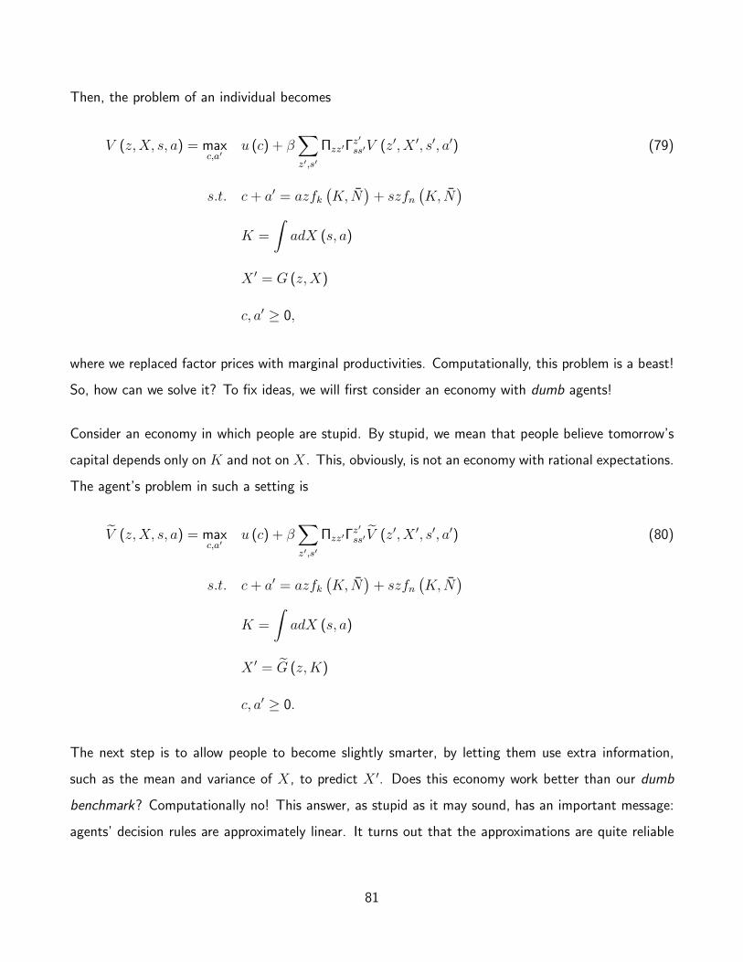
Then, the problem of an individual becomes
V (z,X, s, a) = maxc,a′
u (c) + β∑z′,s′
Πzz′Γz′
ss′V (z′, X ′, s′, a′) (79)
s.t. c + a′ = azfk(K, N
)+ szfn
(K, N
)K =
∫adX (s, a)
X ′ = G (z,X)
c, a′ ≥ 0,
where we replaced factor prices with marginal productivities. Computationally, this problem is a beast!
So, how can we solve it? To fix ideas, we will first consider an economy with dumb agents!
Consider an economy in which people are stupid. By stupid, we mean that people believe tomorrow’s
capital depends only on K and not on X. This, obviously, is not an economy with rational expectations.
The agent’s problem in such a setting is
V (z,X, s, a) = maxc,a′
u (c) + β∑z′,s′
Πzz′Γz′
ss′V (z′, X ′, s′, a′) (80)
s.t. c + a′ = azfk(K, N
)+ szfn
(K, N
)K =
∫adX (s, a)
X ′ = G (z,K)
c, a′ ≥ 0.
The next step is to allow people to become slightly smarter, by letting them use extra information,
such as the mean and variance of X, to predict X ′. Does this economy work better than our dumb
benchmark? Computationally no! This answer, as stupid as it may sound, has an important message:
agents’ decision rules are approximately linear. It turns out that the approximations are quite reliable
81

in the Aiyagari economy!
11.4.2 Linear Approximation Revisited
Let’s now revisit our discussion of linear approximation in the context of the Aiyagari economy. As
we can see in section 11.4.1, solving the heterogeneous agent model with aggregate shocks is compu-
tationally hard. We need to guess a reduced form rule to approximate the distribution for agents to
forecast future prices, and when the model has frictions on several dimensions, there is little we can
say on how to choose such a rule.
We can, however, use a linear approximation to obtain the model’s solution around the steady state.
The idea is as follows: starting from the steady state, we obtain the the impulse responses of the perfect
foresight economy given a sequence of small deterministic shocks. Then, we use these responses to
approximate the behavior of the main aggregates in the economy with heterogeneous agents by adding
small stochastic shocks around the steady state. This method was recently proposed by Boppart,
Krusell, and Mitman (2018).19.
To fix ideas, let’s consider the above Aiyagari economy with a TFP shock z. Let log(zt) follow an
AR(1) process with ρ as the autocorrelation parameter as log(zt) = ρ log(zt−1)+εt. First, compute the
path of the (log of the) shock by letting ε will go up by, say, one unit in period 0. Rewriting the process
in its MA form, we have the full sequence of values (1, ρ, ρ2, ρ3, . . . ) to pin down the TFP path. Then,
we can compute the transition path in the deterministic economy, with the agent taking as given the
sequence of prices. Thus, solving the deterministic path is straightforward: we guess a path for price (or
else we could also guess the path for an aggregate variable), solve the household’s problem backwards
from the final steady state back to initial steady state, and then derive the aggregate implications of the
households’ behavior and update our guess for the price path. This iterative procedure is also standard
and fully nonlinear.
After solving the PFE, we have a sequence of aggregates we care about. We choose one of those,
19 The description of the method below is from that paper with minor modifications.
82
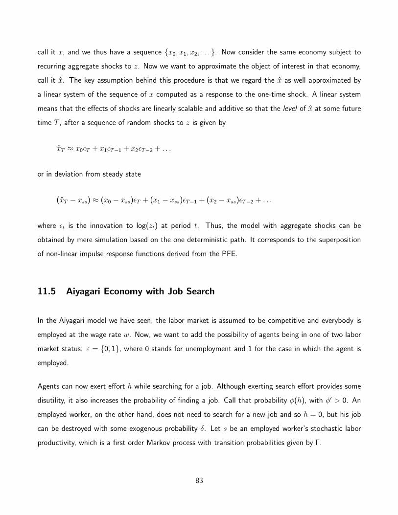
call it x, and we thus have a sequence x0, x1, x2, . . . . Now consider the same economy subject to
recurring aggregate shocks to z. Now we want to approximate the object of interest in that economy,
call it x. The key assumption behind this procedure is that we regard the x as well approximated by
a linear system of the sequence of x computed as a response to the one-time shock. A linear system
means that the effects of shocks are linearly scalable and additive so that the level of x at some future
time T , after a sequence of random shocks to z is given by
xT ≈ x0εT + x1εT−1 + x2εT−2 + . . .
or in deviation from steady state
(xT − xss) ≈ (x0 − xss)εT + (x1 − xss)εT−1 + (x2 − xss)εT−2 + . . .
where εt is the innovation to log(zt) at period t. Thus, the model with aggregate shocks can be
obtained by mere simulation based on the one deterministic path. It corresponds to the superposition
of non-linear impulse response functions derived from the PFE.
11.5 Aiyagari Economy with Job Search
In the Aiyagari model we have seen, the labor market is assumed to be competitive and everybody is
employed at the wage rate w. Now, we want to add the possibility of agents being in one of two labor
market status: ε = 0, 1, where 0 stands for unemployment and 1 for the case in which the agent is
employed.
Agents can now exert effort h while searching for a job. Although exerting search effort provides some
disutility, it also increases the probability of finding a job. Call that probability φ(h), with φ′ > 0. An
employed worker, on the other hand, does not need to search for a new job and so h = 0, but his job
can be destroyed with some exogenous probability δ. Let s be an employed worker’s stochastic labor
productivity, which is a first order Markov process with transition probabilities given by Γ.
83
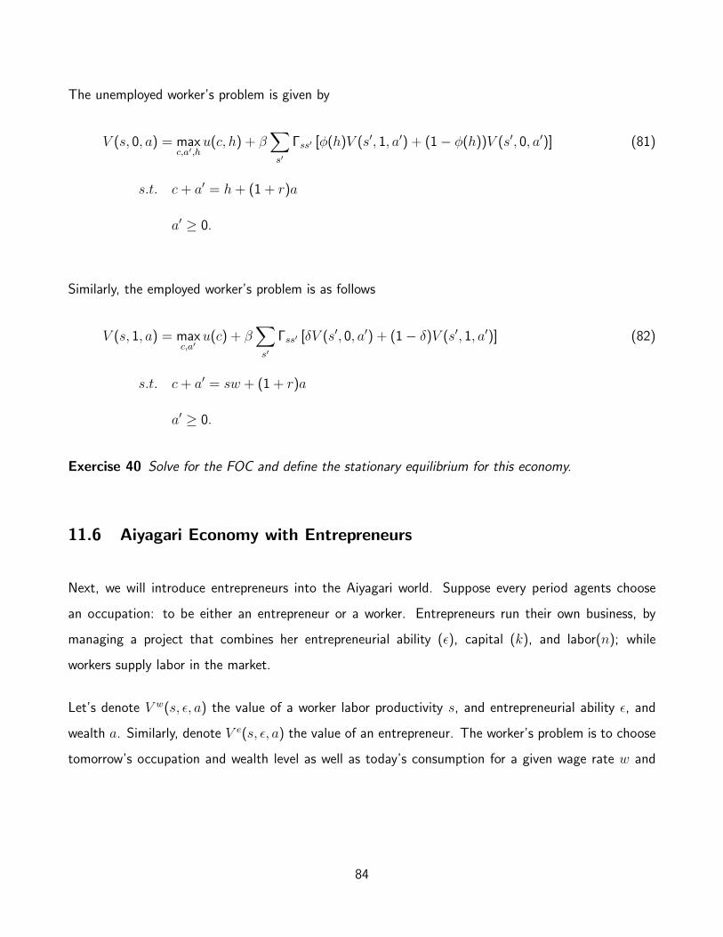
The unemployed worker’s problem is given by
V (s, 0, a) = maxc,a′,h
u(c, h) + β∑s′
Γss′ [φ(h)V (s′, 1, a′) + (1− φ(h))V (s′, 0, a′)] (81)
s.t. c + a′ = h + (1 + r)a
a′ ≥ 0.
Similarly, the employed worker’s problem is as follows
V (s, 1, a) = maxc,a′
u(c) + β∑s′
Γss′ [δV (s′, 0, a′) + (1− δ)V (s′, 1, a′)] (82)
s.t. c + a′ = sw + (1 + r)a
a′ ≥ 0.
Exercise 40 Solve for the FOC and define the stationary equilibrium for this economy.
11.6 Aiyagari Economy with Entrepreneurs
Next, we will introduce entrepreneurs into the Aiyagari world. Suppose every period agents choose
an occupation: to be either an entrepreneur or a worker. Entrepreneurs run their own business, by
managing a project that combines her entrepreneurial ability (ε), capital (k), and labor(n); while
workers supply labor in the market.
Let’s denote V w(s, ε, a) the value of a worker labor productivity s, and entrepreneurial ability ε, and
wealth a. Similarly, denote V e(s, ε, a) the value of an entrepreneur. The worker’s problem is to choose
tomorrow’s occupation and wealth level as well as today’s consumption for a given wage rate w and
84
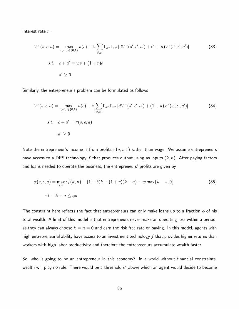
interest rate r.
V w(s, ε, a) = maxc,a′,d∈0,1
u(c) + β∑s′,ε′
Γss′Γεε′ [dVw(s′, ε′, a′) + (1− d)V e(s′, ε′, a′)] (83)
s.t. c + a′ = ws + (1 + r)a
a′ ≥ 0
Similarly, the entrepreneur’s problem can be formulated as follows
V e(s, ε, a) = maxc,a′,d∈0,1
u(c) + β∑s′,ε′
Γss′Γεε′ [dVw(s′, ε′, a′) + (1− d)V e(s′, ε′, a′)] (84)
s.t. c + a′ = π(s, ε, a)
a′ ≥ 0
Note the entrepreneur’s income is from profits π(a, s, ε) rather than wage. We assume entrepreneurs
have access to a DRS technology f that produces output using as inputs (k, n). After paying factors
and loans needed to operate the business, the entrepreneurs’ profits are given by
π(s, ε, a) = maxk,n
εf(k, n) + (1− δ)k − (1 + r)(k − a)− wmaxn− s, 0 (85)
s.t. k − a ≤ φa
The constraint here reflects the fact that entrepreneurs can only make loans up to a fraction φ of his
total wealth. A limit of this model is that entrepreneurs never make an operating loss within a period,
as they can always choose k = n = 0 and earn the risk free rate on saving. In this model, agents with
high entrepreneurial ability have access to an investment technology f that provides higher returns than
workers with high labor productivity and therefore the entrepreenurs accumulate wealth faster.
So, who is going to be an entrepreneur in this economy? In a world without financial constraints,
wealth will play no role. There would be a threshold ε∗ above which an agent would decide to become
85
an entrepreneur. With financial constraints, this changes and wealth now plays an important role.
Wealthy individuals with high entrepreneurial ability will certainly be entrepreneurs, while the poor with
low entrepreneurial ability will become workers. For the other cases, it depends. If the entrepreneurial
ability is persistent, poor individuals with high entrepreneurial ability will save to one day become
entrepreneurs, while rich agents with low entrepreneurial ability will lend their assets and become
workers.
Exercise 41 Solve for the FOC and define the RCE for this economy.
11.7 Other Extensions
There are many more interesting applications. One of these is the economy with unsecured credit and
default decisions. The price of lending will now incorporate the possibility of default. For simplicity,
assume that if the agent decides to default, she live in autarky forever after. In that case, she is
excluded from the financial market and has to consume as much as her labor earnings allow. Let the
individual’s budget constraint in the case of no default be given by
c + q(a′)a′ = a + ws,
where s is labor productivity with transition probabilities given by Γss′ . The problem of an agent is thus
given by
V (s, a) = max
u(ws) + β
∑s′
Γss′V (s′), u(ws + a− q(a′)a′) + β∑s′
Γss′V (s′, a′)
(86)
s.t. a′ ≥ 0,
where V (s′) = 11−βu(ws′) is the value of autarky.
86

12 Monopolistic Competition
12.1 Benchmark Monopolistic Competition
The two most important macroeconomic variables are perhaps output and inflation (movement in the
aggregate price). In this section we take a first step in building a theory of aggregate price. To achieve
this, we need a framework in which firms can choose their own prices and yet the aggregate price is
well defined and easy to handle. The setup of Dixit and Stigltitz (1977) with monopolistic competition
is such a framework.
In an economy with monopolistic competition, firms are sufficiently “different” so that they face a
downward sloping demand curve and thus price discriminate, but also sufficiently small so that they
ignore any strategic interactions with their competitors. We thus assume there are infinitely many
measure 0 firms, each producing one variety of goods. Varieties span on the [0, n] interval and are
imperfect substitutes. Consumers have a “taste for variety” in that they prefer to consume a diversified
bundle of goods (this gives firms some market power as we want). The consumer’s utility function will
have the constant elasticity of substitution (CES) form
u(c(i)i∈[0,n]
)=
(∫ n
0
c(i)σ−1σ di
) σσ−1
where σ is the elasticity of substitution, which is a constant (as the name CES suggests), and c(i) is
the quantity consumed of variety i. For simplicity, we will rename c(i) = ci. For now, we will assume
the agent receives the exogenous nominal income I and is endowed with one unit of time.
We can now solve the household problem
maxcii∈[0,n]
(∫ n
0
cσ−1σ
i di
) σσ−1
s.t.
∫ n
0
picidi ≤ I
87

and derive the FOC, which relates the demand for any varieties i and j as
ci = cj
(pipj
)−σMultiplying both sides by pi and integrating over i, we get the downward sloping demand curve faced
by an individual firm producing variety i as
c∗i =I∫ n
0p1−σj dj
p−σi
We can see that the demand for variety i depends both on the price of variety i and some measure of
“aggregate price”. It is actually convenient to define the aggregate price index P as follows
P =
(∫ n
0
p1−σj dj
) 11−σ
and thus the demand faced by the firm producing variety i can be reformulated as
c∗i =I
P
(piP
)−σwhere the first term is real income and the second is a measure of relative price of variety i.
Exercise 42 Show the following within the monopolistic competition framework above:
1. σ is the elasticity of substitution between varieties.
2. Price index P is the expenditure to purchase a unit-level utility for consumers.
3. Consumer utility is increasing in the number of varieties n.
We are now ready to characterize the firm’s problem. Let’s assume that the production technology is
linear in its inputs and so one unit of output is produced with one unit of labor linearly, i.e., f(nj) = nj.
Let the nominal wage rate be given by W . Also, recall that the quantity of variety j demanded by the
representative agent is such that f(nj) = c∗j . Then, the firm producing variety j solves the following
88

problem
maxpj
π(pj) = pjc∗j(pj)−Wc∗j(pj)
s.t. c∗j =I
P
(piP
)−σRecall that we assume firms are sufficiently small so they would ignore the effect of their own pricing
strategies on aggregate price index P , which greatly simplify the algebra. By solving for the FOC, we
get the straightforward pricing rule
p∗j =σ
σ − 1W ∀j
where σσ−1
is a constant mark-up over the marginal cost, which reflects the elasticity of substitution of
consumers. When varieties are very close substitutes (σ →∞), price just converge to the factor price
W . Not that all firms follow the same pricing strategy, which is independent of the variety j.
We can now define an equilibrium for this simple economy.
Definition 24 A general equilibrium for this environment consists of prices p∗i i∈[0,n], the aggre-
gate price index P , household’s consumption c∗i i∈[0,n] and nominal income I, firm’s labor demand
n∗i i∈[0,n] and profits π∗i i∈[0,n], such that
1. Given prices, c∗i i∈[0,n] solves the household’s problem
2. Given the aggregate price and the input price, π∗i i∈[0,n] and p∗i i∈[0,n] solve the firm’s problem
3. From the firm’s pricing strategy, we have the representative firm condition
P = n1
1−σ p∗i ∀i
89

4. Markets clear
∫c∗i di =
∫n∗i di = 1
I = W +
∫π∗i di
Note that in equilibrium we have c∗i = c, p∗i = p, n∗i = n, π∗i = π for all i.
12.2 Price Rigidity
We now have a simple theory of aggregate price P , which is ultimately shaped by the consumer’s
elasticity of substitution across varieties. However, we are still silent on inflation. To study inflation,
and to have meaningful interactions between output and inflation, we need i) a dynamic model and ii)
some source of nominal frictions.
Nominal frictions mean that nominal variables (things measured in dollars, say, quantity of money) can
affect real variables. The most popular friction used is called price rigidity. With price rigidity, firms
cannot adjust their prices freely. Two commonly used specifications to achieve this in the model are
Rotemberg pricing (menu costs) and Calvo pricing (fairy blessing).
In Rotemberg pricing, firms face adjustment cost φ(pj, p−j ) when changing their prices pj each period.
Using the static model of the previous section (and assuming an exogenous process for the agent’s
nominal endowment It), we can specify the firm’s per period profit under Rotemberg pricing in a
dynamic setup as follows:
πj,t = pj,tc∗j,t −Wtc
∗j,t − φ(pj,t, pj,t−1)It
where c∗jt =
(pj,tPt
)−σItPt
Then each period, firms choose the price that maximizes the expected present discounted value of the
flow profit. Rotemberg is easy in terms of algebra when we assume a quadratic price adjustment cost.
90

However, it generates some fiscal effects that are not so realistic.
A more popular version of price rigidity is the Calvo pricing. It says that instead of facing some
adjustment costs, firms cannot adjust their prices each period with some probability. It’s a bit more
complicated in terms of algebra. We will sketch the problem but leave most of the rest as an exercise.
Each period with probability θ a firm can change its price and with probability 1 − θ the firm is not
allowed to do so. When setting the price, the firm now needs to incorporate the possibility of not being
allowed to adjust its price. Assuming the firm discounts the future at rate 1 + r, its problem at period
t is given by
maxpj,t
∞∑k=0
(1− θ1 + r
)k [pj,tc
∗j,t+k −Wt+kc
∗j,t+k
]s.t. c∗j,t =
(pj,tPt
)−σItPt
Exercise 43 Derive the following for the dynamic model with Calvo pricing
1. Solve the firm’s problem and write the firm’s equilibrium pricing pj,t as a function of present and
future aggregate prices, wages, and endowments: Pt,Wt, It∞t=0.
2. Show that under flexible pricing (θ = 1), the firm’s pricing strategy is identical to the static
model.
3. Show that with price rigidity (θ < 1), the firm’s pricing strategy is identical to the static model
in the steady state with zero inflation.
91
A A Farmer’s Problem: Revisited
Consider the following problem of a farmer that we studied in class:
V (s, a) = maxc,a′
u (c) + β
∑s′
Γss′V (s′, a′)
(87)
s.t. c + qa′ = a + s
c ≥ 0
a′ ≥ 0.
As we discussed, we are in particular interested in the case where β/q < 1. In what follows, we are
going to show that, under monotonicity assumption on the Markov chain governing s, the optimal
policy associated with (87) implies a finite support for the distribution of asset holding of the farmer,
a.20
Before we start the formal proof, suppose smin = 0, and Γssmin> 0, for all s ∈ S. Then, the agent will
optimally always choose a′ > 0. Otherwise, there is a strictly positive probability that the agent enters
tomorrow into state smin, where he has no cash in hand (a′ + smin = 0) and is forced to consume
0, which is extremely painful to him (e.g. when Inada conditions hold for the instantaneous utility).
Hence he will raise his asset holding a′ to insure himself against such risk.
If smin > 0, then the above argument no longer holds, and it is indeed possible for the farmer to choose
zero assets for tomorrow.
Notice that the borrowing constraint a′ ≥ 0 is affecting agent’s asset accumulation decisions, even if
he is away from the zero bound, because he has an incentive to ensure against the risk of getting a
series of bad shocks to s and is forced to 0 asset holdings. This is what we call precautionary savings
motive.
20 This section was prepared by Keyvan Eslami, at the University of Minnesota. This section is essentially a slightvariation on the proofs found in ?. However, he accepts the responsibility for the errors.
92
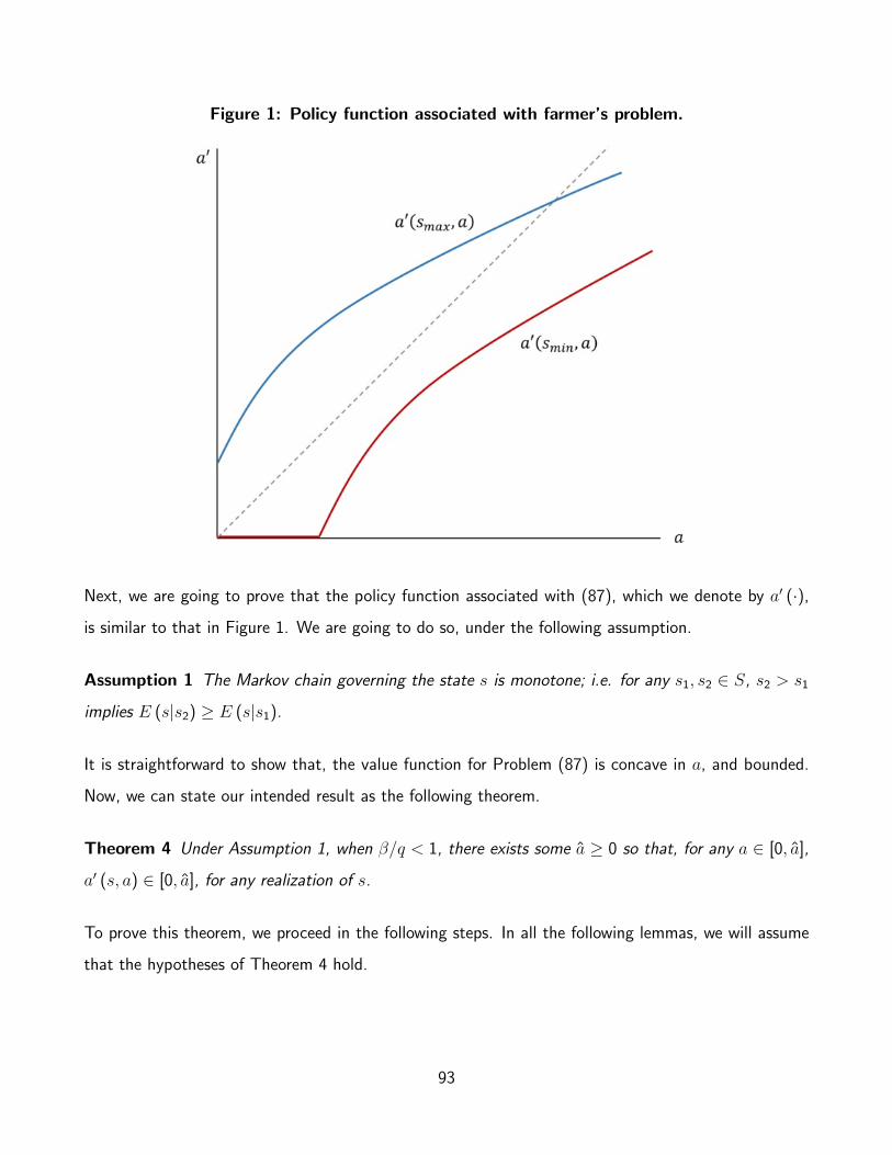
Figure 1: Policy function associated with farmer’s problem.
Next, we are going to prove that the policy function associated with (87), which we denote by a′ (·),
is similar to that in Figure 1. We are going to do so, under the following assumption.
Assumption 1 The Markov chain governing the state s is monotone; i.e. for any s1, s2 ∈ S, s2 > s1
implies E (s|s2) ≥ E (s|s1).
It is straightforward to show that, the value function for Problem (87) is concave in a, and bounded.
Now, we can state our intended result as the following theorem.
Theorem 4 Under Assumption 1, when β/q < 1, there exists some a ≥ 0 so that, for any a ∈ [0, a],
a′ (s, a) ∈ [0, a], for any realization of s.
To prove this theorem, we proceed in the following steps. In all the following lemmas, we will assume
that the hypotheses of Theorem 4 hold.
93
Lemma 1 The policy function for consumption is increasing in a and s;
ca (a, s) ≥ 0 and cs (a, s) ≥ 0.
Proof 1 By the first order condition, we have:
u′ (c (s, a)) ≥ β
q
∑s′
Γss′Va
(s′,a + s− c (s, a)
q
),
with equality, when a + s− c (s, a) > 0.
For the first part of the lemma, suppose a increases, while c (s, a) decreases. Then, by concavity of
u, the left hand side of the above equation increases. By concavity of the value function, V , the right
hand side of this equation decreases, which is a contradiction.
For the the second part, we claim that Va (s, a) is a decreasing function of s. To show this is the case,
firs consider the mapping T as follows:
Tv (s, a) = maxc,a′
u (c) + β
∑s′
Γss′v (s′, a′)
s.t. c + qa′ = a + s
c ≥ 0
a′ ≥ 0.
Suppose vna (s, a) is decreasing in its first argument; i.e. vna (s2, a) < vna (s1, a), for all s2 > s1 and
s1, s2 ∈ S. We claim that, vn+1 = Tvn inherits the same property. To see why, note that for
an+1 (s, a) = a′ (where an+1 is the policy function associated with n’th iteration) we must have:
u′ (a + s− qa′) ≥ β
q
∑s′
Γss′vna (s′, a′) ,
with strict equality when a′ > 0. For a fixed value of a′, an increase in s leads to a decrease in both
sides of this equality, due to the monotonicity assumption of Γ, and the assumption on vna . As a result,
94

we must have
u′(a + s2 − qan+1 (s2, a)
)≤ u′
(a + s1 − qan+1 (s1, a)
),
for all s2 > s1. By Envelope theorem, then:
vn+1a (s2, a) ≤ vn+1
a (s1, a) .
It is straightforward to show that vn converges to the value function V point-wise. Therefore,
Va (s2, a) ≤ Va (s1, a) ,
for all s2 > s1.
Now, note that, by envelope theorem:
Va (s, a) = u′ (c (s, a)) .
As s increases, Va (s, a) decreases. This implies c (s, a) must increase.
Lemma 2 There exists some a ∈ R+, such that ∀a ∈ [0, a], a′ (a, smin) = 0.
Proof 2 It is easy to see that, for a = 0, a′ (a, smin) = 0. First of all, note the first order condition:
uc (c (s, a)) ≥ β
q
∑s′
Γss′uc (c (s′, a′ (s, a))) ,
95

with equality when a′ (s, a) > 0. Under the assumption that β/q < 1, we have:
uc (c (smin, 0)) =β
q
∑s′
Γsmins′uc (c (s′, a′ (smin, 0)))
<∑s′
Γss′uc (c (s′, a′ (smin, 0))) .
By Lemma 1, if a′ = a′ (0, smin) > a = 0, then c (s′, a′) > c (smin, 0) for all s′ ∈ S, which leads to a
contradiction.
Lemma 3 a′ (smin, a) < a, for all a > 0.
Proof 3 Suppose not; then a′ (smin, a) ≥ a > 0 and as we showed in Lemma 2:
uc (c (smin, a)) <∑s′
Γss′uc (c (s′, a′ (smin, a))) .
Contradiction, since a′ (smin, a) ≥ a, and s′ ≥ smin, and the policy function in monotone.
Lemma 4 There exits an upper bound for the agent’s asset holding.
Proof 4 Suppose not; we have already shown that a′ (smin, a) lies below the 45 degree line. Suppose
this is not true for a′ (smax, a); i.e. for all a ≥ 0, a′ (smax, a) > a. Consider two cases.
In the first case, suppose the policy functions for a′ (smax, a) and a′ (smin, a) diverge as a → ∞, so
that, for all A ∈ R+, there exist some a ∈ R+, such that:
a′ (smax, a)− a′ (smin, a) ≥ A.
Since S is finite, this implies, for all C ∈ R+, there exist some a ∈ R+, so that
c (smin, a)− c (smax, a) ≥ C,
which is a contradiction, since c is monotone in s.
96

Next, assume a′ (smax, a) and a′ (smin, a) do not diverge as a→∞. We claim that, as a→∞, c must
grow without bound. This is quite easy to see; note that, by envelope condition:
Va (s, a) = u′ (c (s, a)) .
The fact that V is bounded, then, implies that Va must converge to zero as a → ∞, implying that
c (s, a) must diverge to infinity for all values of s, as a→∞. But, this implies, if a′ (smax, a) > a,
uc (c (smax, a′ (smax, a)))→
∑s′
Γsmaxs′uc (c (s′, a′ (smax, a))) .
As a result, for large enough values of a, we may write:
uc (c (smax, a)) =β
q
∑s′
Γsmaxs′uc (c (s′, a′ (smax, a)))
<∑s′
Γsmaxs′uc (c (s′, a′ (smax, a)))
≈uc (c (smax, a′ (smax, a))) .
But, this implies:
c (smax, a) > c (smax, a′ (smax, a)) ,
which, by monotonicity of policy function, means a > a′ (smax, a), and this is a contradiction.
97