Economic Capital and the Aggregation of Risks using Copulas∗

Andrew Tang and Emiliano A. Valdez†

School of Actuarial StudiesFaculty of Commerce & EconomicsUniversity of New South Wales

Sydney, AUSTRALIA

Abstract

Insurance companies measure and manage capitalacross a broad range of diverse business products.Thus there is a need for the aggregation of the lossesfrom the various business lines whose risk distribu-tions vary. Risk dependencies between losses fromdifferent business lines have long been recognised inthe insurance industry as integral factors driving theinsurer’s aggregate loss process. However, in the past,there has been limited attempt at adequately mod-elling the dependence structure to be factored in theaggregation process for capital determination pur-poses. The current industry standard is to solely uselinear correlations to describe the dependence struc-ture. While being computationally convenient andstraightforward to understand, linear correlations failto capture all the dependence structure that exist be-tween losses from multiple business lines. Other moregeneral dependence modelling techniques such as cop-ulas have become popular recently. In this paper, weaddress the issue of the aggregation of risks using cop-ula models. Copulas can be used to construct jointmultivariate distributions of the losses and provide arather flexible and realistic model of allowing for thedependence structure, while separating the effects ofpeculiar characteristics of the marginal distributionssuch as thickness of tails. This modelling structure al-lows us to explore the impact of dependencies of riskson the total required economic capital. Using numer-ical illustrations based on Australian general insur-ance data, the sensitivities of the capital requirementto the choice of the copula and other modelling as-

∗Keywords: capital at risk, risk measures, risk aggregation,dependence, and copulas.

†The authors wish to acknowledge financial support fromthe Australian Research Council Discovery Grant DP0345036and the UNSW Actuarial Foundation of The Institute of Ac-tuaries of Australia. Please do not quote without authors’permission. Corresponding author’s email address: andy-tang@optusnet.com.au.

sumptions are investigated. The related issue of thediversification benefit from operating multiple busi-ness lines in the context of aggregation of risks bycopulas is also explored. The key conclusion is thatthere is a large variation in the capital requirement aswell as diversification benefit under different copulaassumptions. The results of this paper serve as a re-minder to actuaries and other industry practitionersof the significance of choosing an appropriate aggre-gation model for capital purposes.

1 Introduction

Using the method of copulas, this paper examines theimpact of aggregating risks for purposes of comput-ing economic capital for a multi-line insurance com-pany. Insurance companies measure and manage cap-ital across a broad range of diverse business products.This usually requires the companies to aggregate var-ious business products whose risk distributions vary,that is, the loss distributions of the product lines aredifferent. In recent years, we find that modelling de-pendencies using copulas have become popular in theactuarial, insurance, and finance literature. As wenote in this paper, copulas may be used to constructjoint multivariate distribution of losses and are ratherflexible and realistic in terms of allowing a wide rangeof dependence structure. At the same time, they pro-vide the flexibility of separating the effects of peculiarcharacteristics of the marginal distributions such asthickness of tails. This modelling structure allows theexploration of the impact of dependencies betweenrisks on the total required economic capital.The setting of this paper will be for a general in-

surance company writing multiple lines of business.In developing the analysis, we reasonably assume theAustralian market to be representative of the indus-try in general due to its mature nature. Therefore,many aspects of the paper relate to specific Aus-

Page 1

tralian market conditions.

From the insurer’s perspective, the purpose of cap-ital is to provide a financial cushion for adverse sit-uations when its insurance losses exceed or asset re-turns fall below the levels expected. This cushionfurther enhances the insurer’s ability to continue pay-ing claims and in most instances, to continue writingnew business even under unfavourable financial cir-cumstances. As well put by the International Actu-arial Association (IAA) Insurer Solvency AssessmentWorking Party (2004) which has been primarily re-sponsible for developing solvency standards suitablefor global applications, capital is supposed to be a“rainy day fund, so when bad things happen, there ismoney to cover it.” There is no denying therefore thatthe management of capital forms an integral part ofany insurance company’s risk management.

While there are many forms of capital such as cap-ital required by regulatory authorities and capital re-quired by rating agencies, this paper focuses on theform of capital, namely economic capital, that pro-vides a measure of the amount that the insurancecompany should have at the minimum, to be ableto withstand both expected and unexpected futurelosses. Economic capital is increasingly becoming asignificant area of interest for the internal reportingand management of insurance companies. Mueller(2004) emphasises the distinction between economicand regulatory capital. Economic capital is the bufferset aside against potential losses that reflect risks spe-cific to the insurer while regulatory capital often in-volve formulae based on industry averages and aredesigned for market wide application. Therefore, eco-nomic capital represents a far better measure of aninsurer’s true capital requirements. Giese (2003) alsogives a good overview of this concept and provides adiscussion on recent developments of models for itscalculation. Precise specification for the calculationof economic capital varies from company to company.However, it is generally accepted as the differencebetween the expected value of a risk portfolio anda worst tolerable value at a predetermined tolerablelevel. This paper focuses on a fundamentally equiv-alent definition which is the full amount of a worsttolerable value of a risk portfolio.

This paper addresses the issue of determining theaggregated economic capital of a multi-line insurancecompany when the losses from the several lines ofbusiness are dependent in some sense. We consider aninsurance company with n different lines of business,each of which faces the risk of losing X1,X2, ...,Xn

at the end of a single period. The total company loss

is the random variable

Z = X1 +X2 + · · ·+Xn

where the loss random vector XT = (X1,X2, ...,Xn)has a dependency structure characterized by its jointdistribution using a copula function. It is well-knownthat for a given joint distribution function, say F ,having marginal distributions F1, ..., Fn, there will al-ways be a copula function C that links these mar-ginals to their joint distribution as

F (x1, ..., xn) = C (F1 (x1) , ..., Fn (xn)) .

This result is known as the Sklar’s Theorem (Sklar,1959). For a proof, see Nelsen (1999).For technical completeness, we shall assume that

Xi is a random variable on a well-defined probabilityspace (Ω,F , P ). Suppose further that these randomclaims have a dependency structure characterised bythe joint distribution of the vector XT . Clearly, thetotal capital required for the company, denoted byK,can be determined by the risk measure

ρ : Z → R

which maps the risk Z to the set of real numbers R.In short, K = ρ (Z) ∈ R. Subsequently, we may alsobe interested in the contribution to the total capitalof each line of business although this is beyond thescope of this paper. For a thorough discussion of riskmeasures such as the requirements of a coherent riskmeasure, see Artzner et al. (1999).Risk measures are meant to provide a degree of

magnitude of the severity of a potential loss in a port-folio and are therefore meaningful amounts to hold tocover for the risk exposure. Premium principles areclear examples of risk measures, and these have beenextensively explored in Goovaerts et al. (1984). Afurther reference is the chapter on premium princi-ples in Kaas et al. (2001). Risk measures should notonly serve as a way to learn of the magnitude of risks,but could also be used to compare different risks.Risk measures must be simple to apply and easily

understood. It is for these purposes that we tendedto focus on two widely known and used risk measures:the quantile risk measure, or fondly called the Value-at-Risk (VaR) in financial economics, and the tailconditional expectation (TCE) in this paper. Con-sider a loss random variable whose distribution func-tion we shall denote by FX (·) and survivorship func-tion by FX (·). The random loss X may refer to thetotal claims for an insurance company or to the totalloss in a portfolio of investment for an individual orinstitution.

Page 2

For 0 ≤ q ≤ 1, the q-th quantile risk measure isdefined to be

V aRq (X) = inf (x |FX (x) ≥ q ) . (1)

The TCE is defined to be

TCEq (X) = E (X |X > xq ) (2)

and is interpreted as the expected worst possibleloss. Given the loss will exceed a particular valuexq, generally referred to as the q-th quantile withFX (xq) = 1 − q, the TCE defined in (2) gives theexpected loss that can potentially be experienced.To make a meaningful comparison of numerical val-

ues of the risk measures for sums of dependent ran-dom variables, we draw on results of comonotonicitywhich provides an indication of the strongest possiblepositive dependence structure between random vari-ables. See the papers of Dhaene et al. (2000a, 2000b)on the concept of comonotonicity and their relation-ships to various risk measures. We note the resultsthat the VaR and TCE risk measures for sums ofcomonotonic random variables are in fact additive areessential to the analysis in this paper.Consider a comonotonic random vector, say

XC,T = (Xc1,X

c2 , ...,X

cn) and let the sum of the el-

ements of this vector be Zc = Xc1 +Xc

2 + · · · +Xcn.

It has been demonstrated by Dhaene et al. (2002a,2002b) that V aRq (Z

c) =Pn

i=1 V aRq (Xci ) and that

TCEq (Zc) =Pn

i=1 TCEq (Xci ) .

As a matter of fact, one can therefore view this asthat each business line is a stand alone business hav-ing to establish its own capital requirement. Theseresults therefore imply that in terms of economic cap-ital, if the losses from each business line were per-fectly dependent with one another, then the aggregateeconomic capital required will simply be the sum ofthe economic capital required for each business line.However, there are diversification effects from writ-ing several business lines that are less than perfectlydependent. In this case, the dependence structure isbest specified using copulas.If we then consider the VaR and TCE risk mea-

sures resulting from a particular copula structure, sayV aRq (Z) and TCEq (Z) respectively, then the differ-ences resulting from these measures

V aRq (Zc)− V aRq (Z) and TCEq (Z

c)− TCEq (Z)

provide a measure of the degree of diversificationbenefit derived from constructing the entire portfo-lio. Note that we assume the same marginal dis-tributions hold for the comonotonic copula as wellas the other non-comonotonic copula under consid-eration. This difference will always be non-negative

for any risk measures that do indeed preserve stop-loss order and that are additive for comonotonic risks.Technically, the following result holds: any risk mea-sure ρ that preserves stop-loss order and is additivefor comonotonic random variables is considered sub-additive. That is,

ρ (Z) ≤ ρ (Zc) =nXi=1

ρ (Xci ) =

nXi=1

ρ (Xi) .

For a proof, we suggest consultation of Vanduffel(2004).In other words, from the insurer’s perspective, the

diversification benefit is the difference in the riskmeasure resulting from assuming comonotonic depen-dence to something less than comonotonic. This dif-ference represents the savings in economic capital re-quired due to the diversification of adding businesslines to the portfolio.It is well recognised in the insurance industry that

there is some form of dependence between losses orclaims occurring across the various business lines.Some intuitive explanation to these dependencies hasbeen pointed out in Isaacs (2003). In the industry,catastrophic events such as major storms and earth-quakes usually simultaneously affect more than a sin-gle line of business. Earthquake, for example, canclearly damage both building or housing structuresand at the same time, other insured properties suchas automobiles. It is also believed that general in-flation can cause simultaneous repercussions on sev-eral lines of business, particularly long tail lines. Fur-thermore, in some sense, a single insurance companytypically shares its company philosophy and strategyacross the various business lines. There is, as a conse-quence, some common consistency in the implemen-tation of underwriting rules and guidelines as well asin the establishment of reserves and capital. Theseconsistencies may explain the possible dependenciesthat may exist across the business lines.Dependencies have yet to be accurately factored

into the capital calculations. The theoretical basis ofincorporating the correlation structure is sometimesnot well understood. Some argue that the calcula-tions may be based on the multivariate Normal as-sumption, but even so, this assumption typically re-stricts dependencies of the business lines in the linearsense. This is because correlation explains only lin-ear dependence, but in insurance as well as in someother financial products, other types of dependenciesmay exist. Embrechts et al. (1999) and Priest (2003)both provide such an argument that correlation canbe a source of confusion in modelling dependencies.In an example illustrated by Embrechts et al. (1999),

Page 3

it is possible to have two different probability mod-els that can result from having equal marginals andequal correlation structure. It is for this reason thatthe authors are proponents for modelling a wide de-pendence structure by specifying the structure of themultivariate distribution function with copulas. As amatter of fact, the dependence of a multivariate ran-dom vector is entirely contained in its copula, andas noted by earlier researchers, copulas describe the“scale invariant” dependencies that exist between theelements of the random vector.The rest of the paper has been structured as fol-

lows. Section 2 provides the necessary technical back-ground on copulas. Section 3 discusses the methodol-ogy and assumptions used in developing the numer-ical simulation produced in Section 4 where the nu-merical results of the simulation and their discussionare presented. We conclude this paper in Section 5with a few remarks on the findings, their limitationsand potential direction for future research on the sub-ject of aggregating risks for the purpose of settingcapital requirements.

2 Aggregating Risks usingCopulas

Today, there are several ongoing discussions aboutthe implementation of copula models to account forpossible dependencies between insurance risks. Theseare part of wider analyses into capital requirementsthat have been initiated by various professional bod-ies. First, there is the recent report, that is beingcirculated globally, by the International Actuarial As-sociation (IAA), and assembled by IAA’s Insurer Sol-vency Assessment Working Party (IAA, 2004). Sim-ilarly, a British version of such an assessment titled“Risk and Capital Assessment and Supervision in Fi-nancial Firms” (Creedon et al., 2003) and a Euro-pean Union version titled “Solvency II” is also beingcirculated. We note that these reports generally ad-vocates the importance of recognising and modellingdependencies of multiple risks using copulas. In thissection, we provide some introductory technical back-ground on the subject of copulas.As a mathematical tool to model dependencies,

copulas are not a new invention but is a borrowedconcept from statistics. Used as a tool for under-standing relationships among multivariate outcomes,a copula is a function that links, or couples univariatemarginals to their full multivariate distribution. Cop-ulas were introduced by Sklar (1959) in the context ofprobabilistic metric spaces, a branch of mathematics

that deals with measures. Carriere (2003) provides ashort history and the basic concepts of copulas. Thereis a rapidly developing literature on the statisticalproperties and applications of copulas. As pointedout in Frees and Valdez (1998), there is a variety ofapplications of this tool in actuarial science. See alsoGenest and MacKay (1986a, 1986b), Joe (1997), andNelsen (1999) for further understanding of copulas.Consider u = (u1, ..., un) belonging to the n-cube

[0, 1]n. A copula, C (u), is a function, with sup-

port [0, 1]n and range [0, 1], that is a multivariate cu-mulative distribution function whose univariate mar-ginals are uniform U (0, 1). As a consequence, wesee that C (u1, ..., uk−1, 0, uk+1, ..., un) = 0 and thatC (1, ..., 1, uk, 1, ..., 1) = uk for all k = 1, 2, ..., n. Anycopula function C is therefore the distribution of amultivariate uniform random vector.The significance of copulas in examining the de-

pendence structure of X1,X2, ...,Xn comes from aresult, mainly due to Sklar (1959). It relates themarginal distribution functions to copulas. SupposeX = (X1,X2, ...,Xn)

T is a random vector with jointdistribution function F . According to Sklar (1959),there exists a copula function C such that

F (x1, ..., xn) = C (F1 (x1) , ..., Fn (xn))

where Fk is the kth univariate marginal distributionfunction, for k = 1, 2, ..., n. The function C need notbe unique, but it is unique if the univariate marginalsare absolutely continuous. For absolutely continuousunivariate marginals, the unique copula function isclearly

C (u1, ..., un) = F¡F−11 (x1) , ..., F

−1n (xn)

¢(3)

where F−11 , ..., F−1n denote the quantile functions ofthe univariate marginals F1, ..., Fn. From equation(3), it becomes apparent how the copula “links” or“couples” the joint distribution to its marginals.As pointed out and proven by Embrechts et al.

(1999), one interesting and attractive feature of thecopula representation of dependence which is par-ticularly useful for financial applications, is the in-variance property of copulas. Suppose the randomvector X has copula representation C and the ran-dom vector T (X) be a transformation of X. Thatis, T (X) = (T1 (X1) , T2 (X2) , ..., Tn (Xn))

T whereTi are non-decreasing and continuous functions, fori = 1, 2, ..., n. Then T (X) also has the same copularepresentation C as X.In the remainder of this section, we discuss, with

examples, three classes of copulas: copulas of extremedependence, Archimedean copulas and elliptical cop-ulas.

Page 4

2.1 Copulas of Extreme Dependence

To begin, an example of a copula is the independencecopula which is given by

C (u1, ..., un) = u1 · · · un (4)

and is the copula associated with the joint distribu-tion of independent random variables X1,X2, ...,Xn.This copula is often denoted simply by Π (u).The Frechet bounds for copulas are well-known re-

sults in mathematical statistics. The main results aregiven below and one is directed to consult Frechet(1951, 1957) for more details and discussions of thesebounds. Define

M (u) = min (u1, ..., un)

and

W (u) = max (u1 + ...+ un − n+ 1, 0) .

Then it is always true that for all u in [0, 1]n, we have

W (u) ≤ C (u) ≤M (u) .

For all n ≥ 2, the function M (u) satisfies defini-tion of a copula. For n ≥ 3, the function W (u) isnot a copula. The copula M (u) is a comonotoniccopula and in fact, describes perfect positive depen-dence. For any random variable U that is uniformon [0, 1], the random vector (U,U, ..., U)T has distri-bution function described by the comonotonic cop-ula. Furthermore, if the random vector X has thecomonotonic copula representation, then we say thatits elements X1,X2, ...,Xn are comonotonic randomvariables. Sometimes, it is convenient to place a su-perscript c on the random variables to denote theyare comonotonic, i.e., Xc

1,Xc2, ...,X

cn. The concept

of comonotonicity has had tremendous applicationsin actuarial science, particularly in obtaining boundsfor distribution functions of random variables. SeeDhaene et al. (2002a, 2002b) for many interesting ex-amples and illustrative applications of comonotonic-ity.

2.2 Archimedean Copulas

The use of Lapace transforms can lead us to constructa special type of copulas known as Archimedean cop-ulas. This class of copulas is well discussed in Nelsen(1999). More formally, we say that a copula functionC is Archimedean if it can be written in the form

C (u1, u2, ..., un) = ψ−1 [ψ (u1) + · · ·+ ψ (un)] (5)

for all 0 ≤ u1, ..., un ≤ 1 and for some continuousfunction ψ (often called the generator) satisfying:

(i) ψ (1) = 0;

(ii) ψ is strictly decreasing and convex. That is, forall t ∈ (0, 1), ψ

0(t) < 0 and ψ

00(t) ≥ 0; and

(iii) ψ−1 is completely monotonic on [0,∞).

The “completely monotonic” requirement is a nec-essary and sufficient condition to extend Archimedeancopulas into higher than two dimensions. See Nelsen(1999), for example, for an interesting proof of thisproposition. A function g (t) is said to be completelymonotonic on a specific interval I if it is continuouson the interval and has derivatives of all orders thatalternate in signs. This alternating signs requirementimplies that we must have (−1)k dk

dtkg (t) ≥ 0, for

k = 1, 2, ..., n.This class of copulas has also been extensively stud-

ied by Genest and Mackay (1986) who further demon-strate that this class of copulas possess several desir-able and interesting properties that make them at-tractive for statistical inference and simulation. Inaddition, they are useful for extending copulas tohigher dimensions. Since the copula is completelyspecified once the Archimedean generator is known,another advantage of this Archimedean representa-tion is that when searching for a copula suitable to de-scribe random variables, we reduce the task to search-ing for a single univariate function.

Example 1: Gumbel-Hougaard CopulaUsing the generator defined by ψ (t) = (− log t)α,

this family has members with the following copularepresentation:

C (u1, u2, ..., un) = exp

⎧⎨⎩−"

nXi=1

(− logui)α#1/α⎫⎬⎭ .

(6)It is easy to show that in this case, the inverse of thegenerator is ψ−1 (s) = exp

¡−s1/α

¢and is completely

monotonic for α ≥ 1 making the representation in (6)a valid multivariate copula function.

Example 2: Frank CopulaThe Frank copula has the generator ψ (t) =

− logµe−αt − 1e−α − 1

¶so that its multivariate copula rep-

resentation is:

C (u1, u2, ..., un) = −1

αlog

"1 +

Qni=1 (e

−αui − 1)(e−α − 1)n−1

#.

(7)The inverse of the generator can be expressed asψ−1 (s) = − 1

α log [1 + eαs (e−α − 1)] and is com-pletely monotonic for α > 0. See Frank (1979) and

Page 5

Genest (1987) for details of the characteristics of thiscopula.

Example 3: Cook-Johnson CopulaAnother important example of an Archimedean

copula is the Cook-Johnson copula whose generatoris defined by ψ (t) = t−α − 1 so that its multivariatecopula representation is:

C (u1, u2, ..., un) =

"nXi=1

u−αi − n+ 1

#−1/α. (8)

The inverse of the generator can be expressed asψ−1 (s) = (t+ 1)−1/α and is completely monotonicfor α > 0. These are sometimes called Clayton copu-las and this family has been shown to be important inmultivariate extreme value theory. See, for example,Juri and Wüthrich (2002) for some useful asymptoticresults leading to Clayton copulas.

2.3 Elliptical Copulas

Another very important class of copulas that hasbeen receiving attention in financial applications isthe class of Elliptical copulas. Elliptical copulas aregenerally defined as copulas of elliptical distributions.There are a number of equivalent ways to define ran-dom vectors that belong to the class of elliptical dis-tributions.The n-dimensional vector X is said to have

a multivariate elliptical distribution, written asX v En(µ,Σ,ϕ), if its characteristic function has theform

ϕX (t) = exp(itTµ) · ϕ

¡12t

TΣt¢

for some column-vector µ, n×n positive-definite ma-trix Σ, and some function ϕ(t) called the character-istic generator. Members of the elliptical class has aspecial stochastic representation as follows. Assum-ing X v En(µ,Σ,ϕ) with rank (Σ) = r ≤ n, we canwrite the elliptical random vector as

X = µ+R√ΣU

where U is a uniformly distributed random vectoron u ∈ [−1, 1]r |kuk = 1, the unit sphere, and Ris a non-negative random variable independent of U.The following references, Fang et al. (1987) and Em-brechts et al. (1999), provide comprehensive discus-sions on elliptical distributions. Two further refer-ences for elliptical distributions are Landsman andValdez (2003) and Valdez and Chernih (2003). Thereader is encouraged to consult these references forfurther study about the interesting properties of thisclass of distributions.

We now give some examples of copulas generatedfrom this class of distributions.

Example 1: Gaussian (Normal) CopulaThe copula generated by a multivariate Normal dis-

tribution with linear correlation matrix Σ is given by

C (u1, ..., un) = H¡Φ−1 (u1) , ...,Φ

−1 (un)¢

where H is the joint distribution function of a stan-dard Normal random vector expressed as

H (x1, ..., xn) =

Z xn

−∞

Z xn−1

−∞· · ·Z x1

−∞

1p(2π)n |Σ|

× expµ−12zTΣ−1z

¶dz1 · · · dzn (9)

and Φ−1 (·) is the inverse of a standard Normal distri-bution and Φ (z) =

R z−∞

1√2π· e−w2/2dw. It is critical

to note that Normal copulas have zero tail depen-dence. See Embrechts et al. (2001) for a proof of thisresult.

Example 2: Student-t CopulaThe copula generated by a multivariate Student-t

distribution with linear correlation matrix Σ is givenby

C (u1, ..., un) = Tυ¡t−1υ (u1) , ..., t

−1υ (un)

¢where T is the joint distribution function of a stan-dard Student-t random vector expressed as

Tυ (x1, ..., xn) =Γ¡υ+n2

¢Γ¡υ2

¢(υπ)n/2

p|Σ|

Z xn

−∞

Z xn−1

−∞· ·

· ·Z x1

−∞

µ1 +

1

υzTΣ−1z

¶−(υ+n)/2dz1 · · · dzn (10)

and t−1υ (·) is the inverse of a standard Student-twith tυ (z) =

R z−∞

Γ(υ+12 )Γ(υ2 )(υπ)

1/2 · 1h1+ z2

υ

i υ+12

dz. Unlike

Gaussian copulas, Student-t copulas have non-zerotail dependence. Again, a proof can be found in Em-brechts et al. (2001) for this result.

Example 3: Cauchy CopulaThe Cauchy copula is actually a special case of

the Student-t copula where the degrees of freedom isυ = 1. Thus, the copula generated by a multivariateCauchy distribution with linear correlation matrix Σis given by

C (u1, ..., un) = T1¡t−11 (u1) , ..., t

−11 (un)

¢

Page 6

where T1 then is the joint distribution function of astandard Cauchy random vector expressed as

T1 (x1, ..., xn) =Γ¡n+12

¢Γ¡12

¢(π)n/2

p|Σ|

Z xn

−∞

Z xn−1

−∞· ·

· ·Z x1

−∞

¡1 + zTΣ−1z

¢−(n+1)/2dz1 · · · dzn (11)

and t−11 (·) is the inverse of a standard Cauchy distri-bution with t1 (z) =

R z−∞

1π ·³

11+w

´2dw. Due to its

relationship with the Student-t copulas, we deducethat Cauchy copulas also have non-zero tail depen-dence.

Embrechts et al. (2001) provides overviews of allthree examples of elliptical copulas and the reader isdirected to that paper for further discussion.

3 Numerical Simulation

The primary goal of this paper is to assess the eco-nomic capital required for a multi-line insurer undervarious copula assumptions. Also, we try to quantifythe diversification benefit for the same insurer fromholding capital against the aggregate loss comparedto holding the aggregate capital against losses fromeach business line under the different copulas. Wediscuss the existence of this diversification benefit interms of capital in the Introduction section and havesuggested a reference in Vanduffel (2004) for a proof.A SAS program written using the Interactive Ma-

trix Language (IML) procedure was developed to sim-ulate and aggregate the prospective one year loss ratiodistributions for each business line. For each line ofbusiness, 1,000 loss ratio simulations were generatedfor each copula to represent the sampling distribu-tion. Appendix A provides the algorithm used forthis simulation and the SAS program code is docu-mented in Tang (2004).The simulation performed in this paper have been

motivated by historical data of losses for the aggre-gate Australian industry. First, we note that our sim-ulation is based on loss ratios. The gross loss ratio(LR) defined as the ratio of the gross incurred claimsand earned premium is a proxy for loss variables tomake the measurement dimension invariant. The lossratio for the period t derived from business unit i isdefined as

LRi,t =ICi,t

EPi,t

where ICi,t and EPi,t denote respectively the in-curred claims and earned premium from line i during

period t. The loss ratio is in essence a standardisedclaims measure, in this case by a measure of the expo-sure to risk - gross earned premium. This standard-isation allows valid comparison between losses frombusiness lines with different levels of risk exposure.For each copula, we calculate the distribution of

the aggregate loss ratios at the company level takingthe weighted average of each line’s loss ratios accord-ing to pre-specified proportion of earned premium.The weighted averages are valid representations of theaggregate loss ratios due to the following argument.Suppose the following additional notation: LRt de-notes the aggregate loss ratio; ICt denotes the aggre-gate incurred claims; and EPt denotes the aggregateearned premium; at time t, and there are n lines ofbusiness in total.

LRt =ICt

EPt=

Pni=1 ICi,tPni=1EPi,t

=

Pni=1

ICi,tEPi,t

∗EPi,tPni=1EPi,t

=nXi=1

LRi,t ∗EPi,tPni=1EPi,t

=nXi=1

LRi,t ∗wi,t

where wi,t =EPi,tPni=1 EPi,t

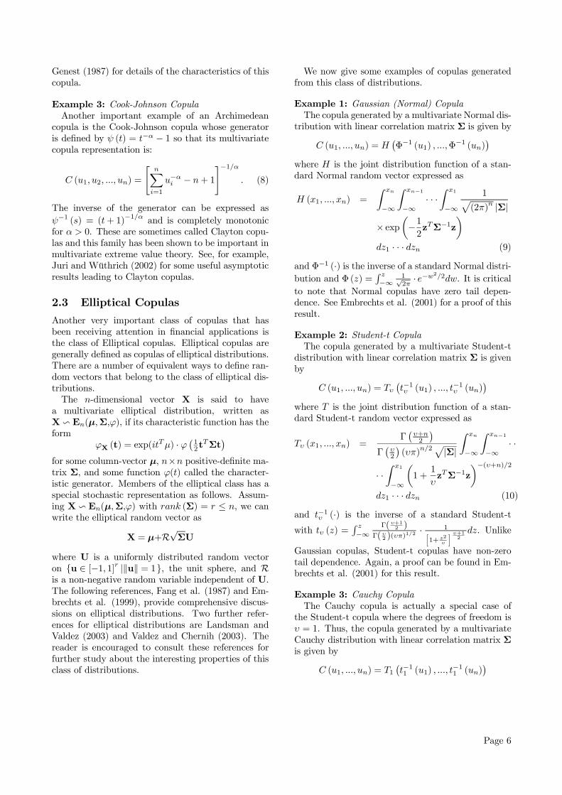
represents the weight of linei in period t by earned premium. Figure 1 displaysthe time series of the observed historical loss ratios.

3.1 Data Supporting AssumptionsUsed for Simulation

Historical loss ratios for the aggregate Australian in-dustry is used to derive the inter business line correla-tion and marginal distribution required as inputs forthe parameterisation of the various copulas. In otherwords, the Australian industry is chosen as a proxyfor all general insurance industries. This is a reason-able assumption due to three factors. First, the Aus-tralian industry is mature by global standards and of-fers a comprehensive, if not exhaustive range of prod-ucts. Second, despite the country’s relatively smallpopulation, the Australian general insurance marketis disproportionally large on a per capita basis, ac-counting for several percentage points of the globalmarket. This leads to Australian practices being rep-resentative of world standards and in fact, are often atthe forefront of innovations in the industry. Finally,despite some concern over the degree of concentrationin the current market due to rationalisation acrossthe industry over the past decade, historically overthe period from which the data was collected, therehas been a reasonable amount of actively operatingissuers, and hence competition, for a market of thissize.

Page 7

S2.

92

S1.

93

S2.

93

S1.

94

S2.

94

S1.

95

S1.

96

S2.

96

S1.

97

S2.

97

S1.

98

S2.

98

S1.

99

S2.

99

S1.

00

S2.

00

S1.

01

S2.

01

S1.

02

0

1

2

MotorCTPHouseholdLiabilityFire...ISR

Loss

Rat

ios

Period

Figure 1: Historical Loss Ratios

0.50

0.70

0.90

1.10

1.30

Motor

0

1

2

3

4

5

0.50

0.70

0.90

1.10

1.30

Household

0

2

4

6

8

0.40

0.52

0.64

0.76

0.88

1.00

1.12

1.24

1.36

1.48

Fire & ISR

0

1

2

3

4

0.40

0.52

0.64

0.76

0.88

1.00

1.12

1.24

1.36

1.48

Liability

0

1

2

3

0.40

0.52

0.64

0.76

0.88

1.00

1.12

1.24

1.36

1.48

1.60

CTP

0

1

2

3

4

Figure 2: Distributions of Historical Loss Ratios

Page 8

3.1.1 Data Source and Collection Period

All historical data used in this paper are presented inthe various semi-annual issues of APRA and formerOffice of the Insurance Commissioner publications aslisted below.

• APRA, Selected Statistics on the General Insur-ance Industry, December 1996 — June 2002

• Office of the Insurance Commissioner, SelectedStatistics on the General Insurance Industry —Total Industry In and Outside of Australia, De-cember 1992 — June 1996

Except where indicated, these publications reportaggregate general insurance industry data that havebeen reported during the 12 month period prior tothe publication dates of 30 June and 31 December ofeach year.The Office of the Insurance Commissioner pub-

lished similar industry statistics dating back to the1970s. However, we find the data format prior to De-cember 1992 is materially different to all subsequentperiods and hence decided not to include these foruse in this paper. The reason for this difference wasdue to a change in reporting procedures by the insur-ance companies to the regulatory authority and thedetails can be found in the June 1992 issue of theSelected Statistics (Office of the Insurance Commis-sioner, 1992).Between December 1992 and June 2002, data for 19

periods, from June and December of each year werecollected. At the time of writing, access to the De-cember 1995 issue of the Selected Statistics was un-available and hence there is a discontinuity of the dataat this date. Also worthy of note are the data pointsfrom December 1992 and November 1997 (substitut-ing December 1997). The data for December 1992is for the 6 month period ending 31 December 1992inclusive of 30 June 1992, and the data for November1997 is for the 11 month period ending 30 Novem-ber 1997. These are different from all the other datapoints in that they did not cover a full 12 month pe-riod. In particular, the difference is quantitativelysignificant for November 1997 due to its exclusion ofthe month of December during which numerous com-panies report. For this period, incurred claims andearned premium were respectively 42% and 40% lowerthan those of the subsequent period (June 1998). Wedo not omit either of these anomalies in the data setas the quantity of interest is ultimately the loss ratio,which as a ratio between incurred claims and earned

Line of Earned Marketbusiness Category Premium * ShareMotor Short tail 4,830,180 31.1%Household Short tail 2,460,770 15.8%Fire & ISR Intermed. tail 1,655,224 10.6%Liability Long tail 2,429,945 15.6%CTP Long tail 1,975,778 12.7%Source: APRA (2002); * (A$,000)

Table 1: Business Line Assumptions and their MarketShare

premium, is not materially impacted on by variationsin the length of time coverage.Since in general, annual data collected semi-

annually has been used, there was some initial con-cern about the overlapping of the collection periodand that this will distort the dependence structure.For example, the June 1998 data refers to the periodfrom 1 July 1997 to 30 June 1998 whereas the De-cember 1998 data refers to the period from 1 January1998 to 31 December 1998, hence the period between1 January 1998 and 30 June 1998 are included in bothof the data points. On further consideration, we de-cided that this will not impact on the results as onlythe characteristics (correlation and distribution) be-tween lines rather than serially through time are ofconcern in this paper.

3.1.2 Mapping to Business Lines

We decided that for the purpose of this paper thegeneral insurance industry is to consist of a totalof five business lines. This number of lines is largeenough to allow for analysis in adequate depth with-out causing unnecessary complications in the analysisprocess. In order to create a realistic and represen-tative reflection of the industry, the top five businesslines by earned premium from the June 2002 SelectedStatistics (APRA, 2002) are chosen for analysis. Abroad mix of business lines resulted from this selec-tion criterion which also fulfils the requirement fora good representation of the industry. Of the fivebusiness lines chosen, two are short tail, one inter-mediate tail and two are long tail lines. This selec-tion criterion is broadly in line with the methodologyof previous studies where similar empirical data bybusiness lines were used. For an example, see Sherrisand Sutherland-Wong (2004). Table 1 outlines thebusiness lines assumed and their market share. Thisselection represents approximately 86% (excluding in-wards reinsurance) of the aggregate market activitiesas measured by earned premium and hence agrees

Page 9

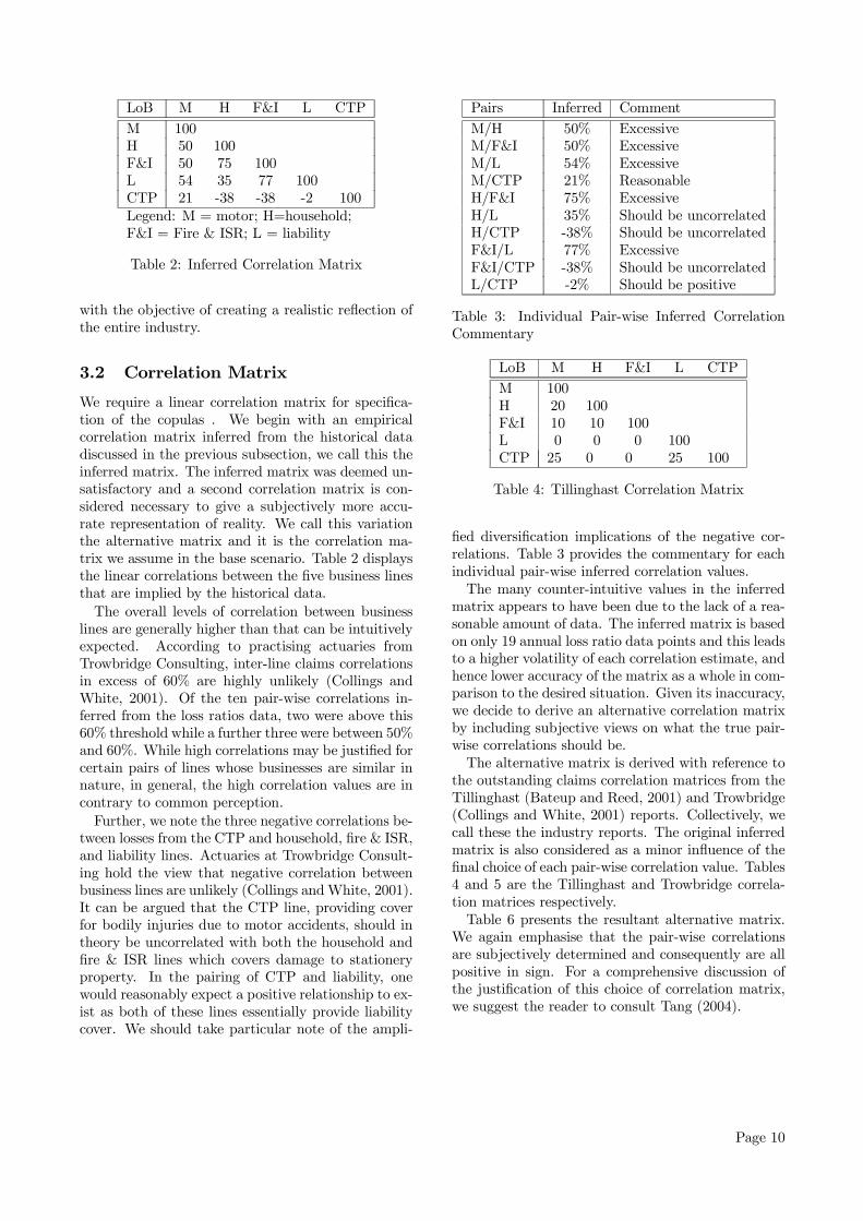
LoB M H F&I L CTPM 100H 50 100F&I 50 75 100L 54 35 77 100CTP 21 -38 -38 -2 100Legend: M = motor; H=household;F&I = Fire & ISR; L = liability

Table 2: Inferred Correlation Matrix

with the objective of creating a realistic reflection ofthe entire industry.

3.2 Correlation Matrix

We require a linear correlation matrix for specifica-tion of the copulas . We begin with an empiricalcorrelation matrix inferred from the historical datadiscussed in the previous subsection, we call this theinferred matrix. The inferred matrix was deemed un-satisfactory and a second correlation matrix is con-sidered necessary to give a subjectively more accu-rate representation of reality. We call this variationthe alternative matrix and it is the correlation ma-trix we assume in the base scenario. Table 2 displaysthe linear correlations between the five business linesthat are implied by the historical data.The overall levels of correlation between business

lines are generally higher than that can be intuitivelyexpected. According to practising actuaries fromTrowbridge Consulting, inter-line claims correlationsin excess of 60% are highly unlikely (Collings andWhite, 2001). Of the ten pair-wise correlations in-ferred from the loss ratios data, two were above this60% threshold while a further three were between 50%and 60%. While high correlations may be justified forcertain pairs of lines whose businesses are similar innature, in general, the high correlation values are incontrary to common perception.Further, we note the three negative correlations be-

tween losses from the CTP and household, fire & ISR,and liability lines. Actuaries at Trowbridge Consult-ing hold the view that negative correlation betweenbusiness lines are unlikely (Collings andWhite, 2001).It can be argued that the CTP line, providing coverfor bodily injuries due to motor accidents, should intheory be uncorrelated with both the household andfire & ISR lines which covers damage to stationeryproperty. In the pairing of CTP and liability, onewould reasonably expect a positive relationship to ex-ist as both of these lines essentially provide liabilitycover. We should take particular note of the ampli-

Pairs Inferred CommentM/H 50% ExcessiveM/F&I 50% ExcessiveM/L 54% ExcessiveM/CTP 21% ReasonableH/F&I 75% ExcessiveH/L 35% Should be uncorrelatedH/CTP -38% Should be uncorrelatedF&I/L 77% ExcessiveF&I/CTP -38% Should be uncorrelatedL/CTP -2% Should be positive

Table 3: Individual Pair-wise Inferred CorrelationCommentary

LoB M H F&I L CTPM 100H 20 100F&I 10 10 100L 0 0 0 100CTP 25 0 0 25 100

Table 4: Tillinghast Correlation Matrix

fied diversification implications of the negative cor-relations. Table 3 provides the commentary for eachindividual pair-wise inferred correlation values.The many counter-intuitive values in the inferred

matrix appears to have been due to the lack of a rea-sonable amount of data. The inferred matrix is basedon only 19 annual loss ratio data points and this leadsto a higher volatility of each correlation estimate, andhence lower accuracy of the matrix as a whole in com-parison to the desired situation. Given its inaccuracy,we decide to derive an alternative correlation matrixby including subjective views on what the true pair-wise correlations should be.The alternative matrix is derived with reference to

the outstanding claims correlation matrices from theTillinghast (Bateup and Reed, 2001) and Trowbridge(Collings and White, 2001) reports. Collectively, wecall these the industry reports. The original inferredmatrix is also considered as a minor influence of thefinal choice of each pair-wise correlation value. Tables4 and 5 are the Tillinghast and Trowbridge correla-tion matrices respectively.Table 6 presents the resultant alternative matrix.

We again emphasise that the pair-wise correlationsare subjectively determined and consequently are allpositive in sign. For a comprehensive discussion ofthe justification of this choice of correlation matrix,we suggest the reader to consult Tang (2004).

Page 10

LoB M H F&I L CTPM 100H 20 100F&I 20 40 100L 0 0 0 100CTP 0 0 0 20 100

Table 5: Trowbridge Correlation Matrix

LoB M H F&I L CTPM 100H 20 100F&I 20 50 100L 10 0 20 100CTP 20 0 0 25 100

Table 6: Alternative Correlation Matrix

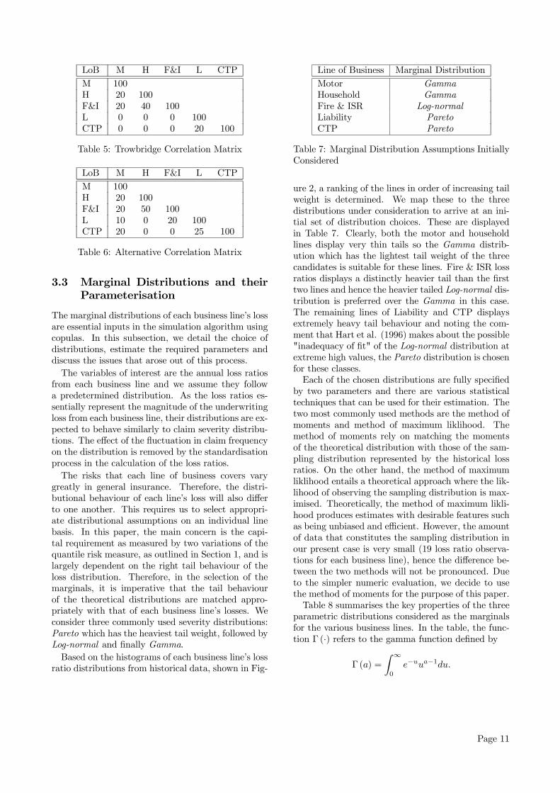
3.3 Marginal Distributions and theirParameterisation

The marginal distributions of each business line’s lossare essential inputs in the simulation algorithm usingcopulas. In this subsection, we detail the choice ofdistributions, estimate the required parameters anddiscuss the issues that arose out of this process.The variables of interest are the annual loss ratios

from each business line and we assume they followa predetermined distribution. As the loss ratios es-sentially represent the magnitude of the underwritingloss from each business line, their distributions are ex-pected to behave similarly to claim severity distribu-tions. The effect of the fluctuation in claim frequencyon the distribution is removed by the standardisationprocess in the calculation of the loss ratios.The risks that each line of business covers vary

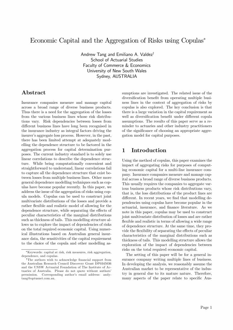
greatly in general insurance. Therefore, the distri-butional behaviour of each line’s loss will also differto one another. This requires us to select appropri-ate distributional assumptions on an individual linebasis. In this paper, the main concern is the capi-tal requirement as measured by two variations of thequantile risk measure, as outlined in Section 1, and islargely dependent on the right tail behaviour of theloss distribution. Therefore, in the selection of themarginals, it is imperative that the tail behaviourof the theoretical distributions are matched appro-priately with that of each business line’s losses. Weconsider three commonly used severity distributions:Pareto which has the heaviest tail weight, followed byLog-normal and finally Gamma.Based on the histograms of each business line’s loss

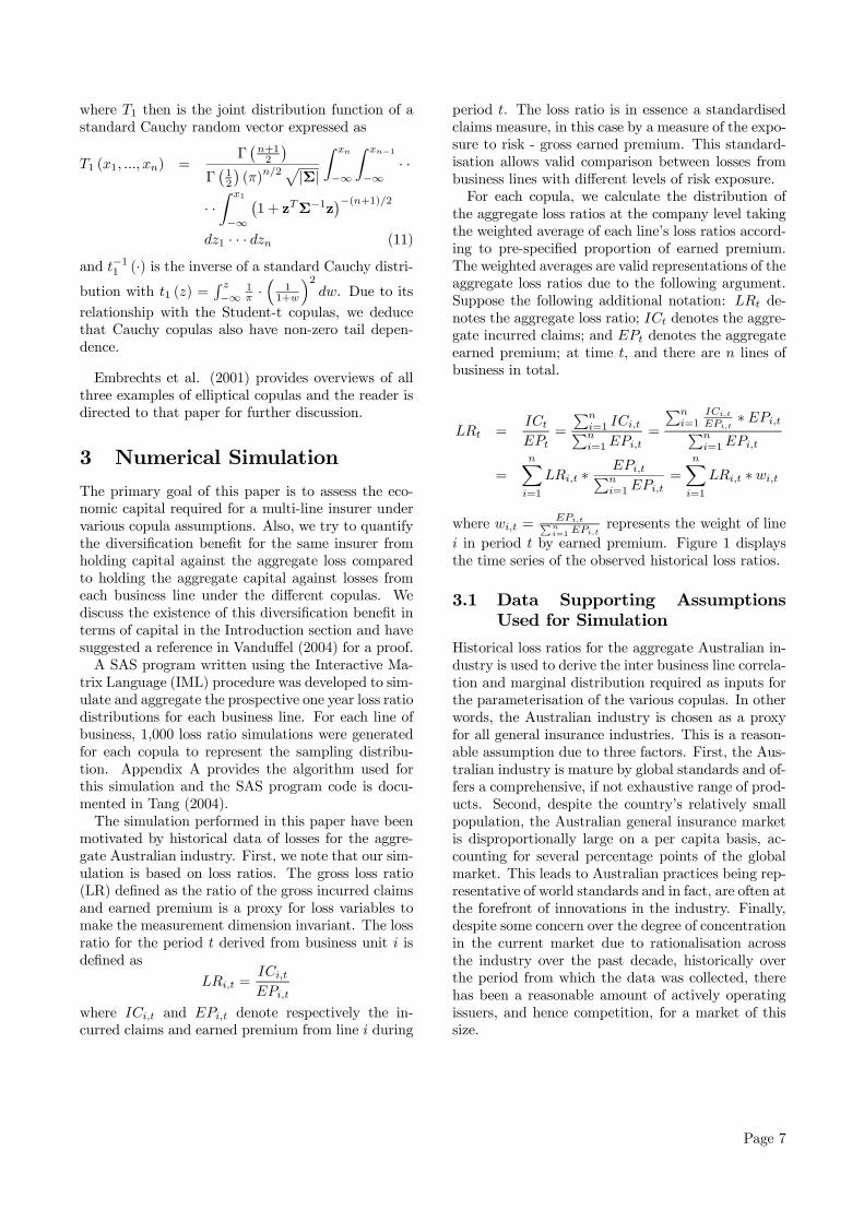
ratio distributions from historical data, shown in Fig-

Line of Business Marginal DistributionMotor GammaHousehold GammaFire & ISR Log-normalLiability ParetoCTP Pareto

Table 7: Marginal Distribution Assumptions InitiallyConsidered

ure 2, a ranking of the lines in order of increasing tailweight is determined. We map these to the threedistributions under consideration to arrive at an ini-tial set of distribution choices. These are displayedin Table 7. Clearly, both the motor and householdlines display very thin tails so the Gamma distrib-ution which has the lightest tail weight of the threecandidates is suitable for these lines. Fire & ISR lossratios displays a distinctly heavier tail than the firsttwo lines and hence the heavier tailed Log-normal dis-tribution is preferred over the Gamma in this case.The remaining lines of Liability and CTP displaysextremely heavy tail behaviour and noting the com-ment that Hart et al. (1996) makes about the possible"inadequacy of fit" of the Log-normal distribution atextreme high values, the Pareto distribution is chosenfor these classes.Each of the chosen distributions are fully specified

by two parameters and there are various statisticaltechniques that can be used for their estimation. Thetwo most commonly used methods are the method ofmoments and method of maximum liklihood. Themethod of moments rely on matching the momentsof the theoretical distribution with those of the sam-pling distribution represented by the historical lossratios. On the other hand, the method of maximumliklihood entails a theoretical approach where the lik-lihood of observing the sampling distribution is max-imised. Theoretically, the method of maximum likli-hood produces estimates with desirable features suchas being unbiased and efficient. However, the amountof data that constitutes the sampling distribution inour present case is very small (19 loss ratio observa-tions for each business line), hence the difference be-tween the two methods will not be pronounced. Dueto the simpler numeric evaluation, we decide to usethe method of moments for the purpose of this paper.Table 8 summarises the key properties of the three

parametric distributions considered as the marginalsfor the various business lines. In the table, the func-tion Γ (·) refers to the gamma function defined by

Γ (a) =

Z ∞0

e−uua−1du.

Page 11

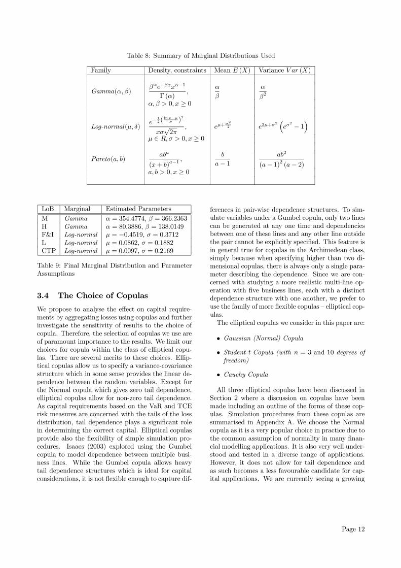
Table 8: Summary of Marginal Distributions Used

Family Density, constraints Mean E (X) Variance V ar (X)

Gamma(α, β)βαe−βxxα−1

Γ (α),

α

β

α

β2

α, β > 0, x ≥ 0

Log-normal(µ, δ)e−

12(

lnx−µσ )

2

xσ√2π

, eµ+σ2

2 e2µ+σ2³eσ

2 − 1´

µ ∈ R,σ > 0, x ≥ 0

Pareto(a, b)aba

(x+ b)a−1,

b

a− 1ab2

(a− 1)2 (a− 2)a, b > 0, x ≥ 0

LoB Marginal Estimated ParametersM Gamma α = 354.4774, β = 366.2363H Gamma α = 80.3886, β = 138.0149F&I Log-normal µ = −0.4519, σ = 0.3712L Log-normal µ = 0.0862, σ = 0.1882CTP Log-normal µ = 0.0097, σ = 0.2169

Table 9: Final Marginal Distribution and ParameterAssumptions

3.4 The Choice of Copulas

We propose to analyse the effect on capital require-ments by aggregating losses using copulas and furtherinvestigate the sensitivity of results to the choice ofcopula. Therefore, the selection of copulas we use areof paramount importance to the results. We limit ourchoices for copula within the class of elliptical copu-las. There are several merits to these choices. Ellip-tical copulas allow us to specify a variance-covariancestructure which in some sense provides the linear de-pendence between the random variables. Except forthe Normal copula which gives zero tail dependence,elliptical copulas allow for non-zero tail dependence.As capital requirements based on the VaR and TCErisk measures are concerned with the tails of the lossdistribution, tail dependence plays a significant rolein determining the correct capital. Elliptical copulasprovide also the flexibility of simple simulation pro-cedures. Isaacs (2003) explored using the Gumbelcopula to model dependence between multiple busi-ness lines. While the Gumbel copula allows heavytail dependence structures which is ideal for capitalconsiderations, it is not flexible enough to capture dif-

ferences in pair-wise dependence structures. To sim-ulate variables under a Gumbel copula, only two linescan be generated at any one time and dependenciesbetween one of these lines and any other line outsidethe pair cannot be explicitly specified. This feature isin general true for copulas in the Archimedean class,simply because when specifying higher than two di-mensional copulas, there is always only a single para-meter describing the dependence. Since we are con-cerned with studying a more realistic multi-line op-eration with five business lines, each with a distinctdependence structure with one another, we prefer touse the family of more flexible copulas — elliptical cop-ulas.The elliptical copulas we consider in this paper are:

• Gaussian (Normal) Copula

• Student-t Copula (with n = 3 and 10 degrees offreedom)

• Cauchy Copula

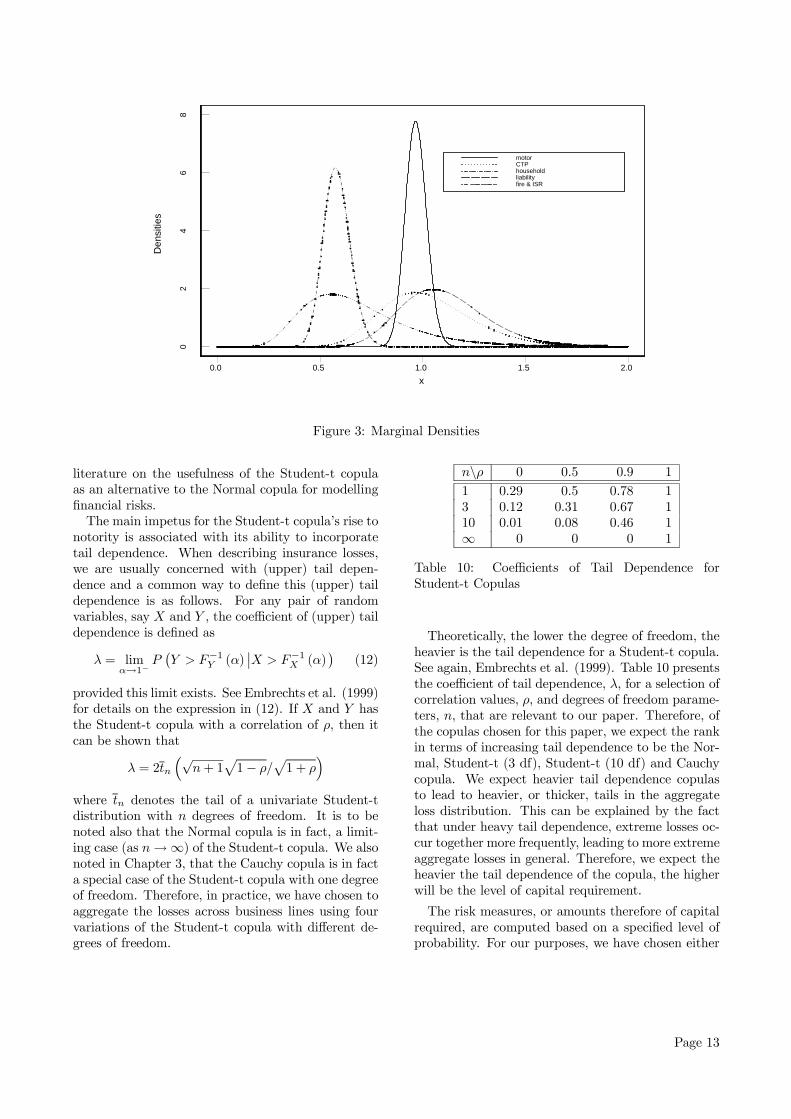
All three elliptical copulas have been discussed inSection 2 where a discussion on copulas have beenmade including an outline of the forms of these cop-ulas. Simulation procedures from these copulas aresummarised in Appendix A. We choose the Normalcopula as it is a very popular choice in practice due tothe common assumption of normality in many finan-cial modelling applications. It is also very well under-stood and tested in a diverse range of applications.However, it does not allow for tail dependence andas such becomes a less favourable candidate for cap-ital applications. We are currently seeing a growing

Page 12

0.0 0.5 1.0 1.5 2.0x

02

46

8

Den

sitie

smotorCTPhouseholdliabilityfire & ISR

Figure 3: Marginal Densities

literature on the usefulness of the Student-t copulaas an alternative to the Normal copula for modellingfinancial risks.The main impetus for the Student-t copula’s rise to

notority is associated with its ability to incorporatetail dependence. When describing insurance losses,we are usually concerned with (upper) tail depen-dence and a common way to define this (upper) taildependence is as follows. For any pair of randomvariables, say X and Y , the coefficient of (upper) taildependence is defined as

λ = limα→1−

P¡Y > F−1Y (α)

¯X > F−1X (α)

¢(12)

provided this limit exists. See Embrechts et al. (1999)for details on the expression in (12). If X and Y hasthe Student-t copula with a correlation of ρ, then itcan be shown that

λ = 2tn

³√n+ 1

p1− ρ/

p1 + ρ

´where tn denotes the tail of a univariate Student-tdistribution with n degrees of freedom. It is to benoted also that the Normal copula is in fact, a limit-ing case (as n→∞) of the Student-t copula. We alsonoted in Chapter 3, that the Cauchy copula is in facta special case of the Student-t copula with one degreeof freedom. Therefore, in practice, we have chosen toaggregate the losses across business lines using fourvariations of the Student-t copula with different de-grees of freedom.

n\ρ 0 0.5 0.9 11 0.29 0.5 0.78 13 0.12 0.31 0.67 110 0.01 0.08 0.46 1∞ 0 0 0 1

Table 10: Coefficients of Tail Dependence forStudent-t Copulas

Theoretically, the lower the degree of freedom, theheavier is the tail dependence for a Student-t copula.See again, Embrechts et al. (1999). Table 10 presentsthe coefficient of tail dependence, λ, for a selection ofcorrelation values, ρ, and degrees of freedom parame-ters, n, that are relevant to our paper. Therefore, ofthe copulas chosen for this paper, we expect the rankin terms of increasing tail dependence to be the Nor-mal, Student-t (3 df), Student-t (10 df) and Cauchycopula. We expect heavier tail dependence copulasto lead to heavier, or thicker, tails in the aggregateloss distribution. This can be explained by the factthat under heavy tail dependence, extreme losses oc-cur together more frequently, leading to more extremeaggregate losses in general. Therefore, we expect theheavier the tail dependence of the copula, the higherwill be the level of capital requirement.

The risk measures, or amounts therefore of capitalrequired, are computed based on a specified level ofprobability. For our purposes, we have chosen either

Page 13

q = 97.5% or q = 99.5%. These arbitrary confidencelevels are chosen to be consistent with the range im-plied by current industry practice for capital purposesand are confirmed with practising actuaries. In par-ticular, q = 99.5% is chosen to facilitate the consis-tent comparison of our results with that of APRA’sPrescribed Method (PM) in order to answer researchquestion 6 of this paper.Given the distribution of prospective loss ratios

from the output of the SAS program, we can read-ily calculate the VaR and TCE at the chosen levels ofq in Microsoft Excel. The VaR measure is calculatedas the point on the ranked loss ratios distributionthat corresponds to the particular level of q. Thatis, for each output distribution, of the 1000 simulatedloss ratios, V aR97.5% corresponds to the 975th valueif the distribution is ranked in increasing magnitude.Similarly, V aR99.5% corresponds to the 995th value inthe same ranked distribution. To calculate the TCE,we simply take the arithmetic average, or expectedvalue, of the values subsequent to the value corre-sponding to the VaR measure. Therefore, TCE97.5%is calculated as the average of the 976th to 1000thvalue of the ranked loss ratios distribution and sim-ilarly, TCE97.5% is calculated as the average of the996th to 1000th value of teh ranked loss ratios distri-bution. The respective VaR and TCE measures canbe calculated for the distribution of loss ratios foreach business line as well as for the insurer’s portfolioin aggregate. Since the SAS program automaticallyaggregates the loss ratios from each business line, theprocedure for calculating the VaR and TCE measuredoes not change for the aggregate portfolio case. Thatis, the procedure is simply applied to the distributionof loss ratios for the aggregate portfolio rather thanthe distribution for each business line.

4 Results of Simulation

Using the procedure as outlined in the previous sec-tion, for each of the five chosen copula models, wegenerated 1,000 observations of the loss ratios for eachbusiness line. These represent the loss, per unit ofpremium, distribution for each business line underthe different copula assumptions.

4.1 The Simulated Loss Ratios

First, let us examine the resulting loss ratios, for eachcopula model, in the case where we assume the alter-native correlation matrix as described in section 3.2.On their own, each line of business do not lead toany meaningful results in terms of the present inter-

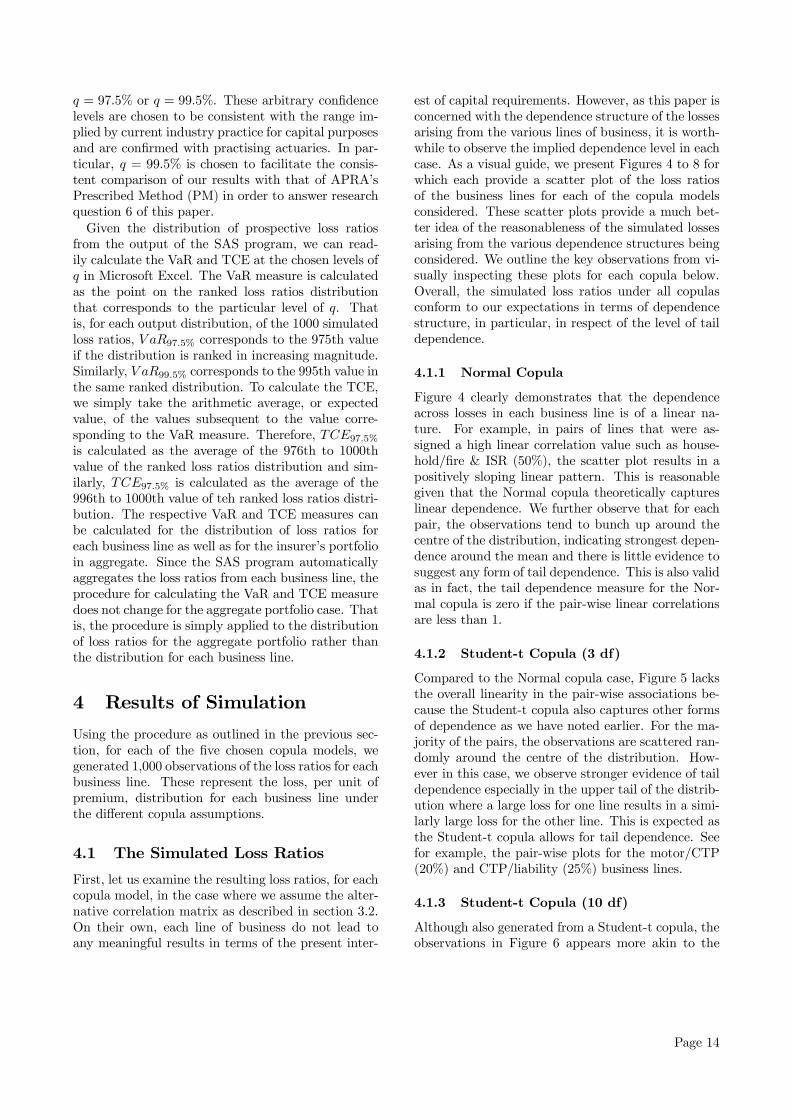
est of capital requirements. However, as this paper isconcerned with the dependence structure of the lossesarising from the various lines of business, it is worth-while to observe the implied dependence level in eachcase. As a visual guide, we present Figures 4 to 8 forwhich each provide a scatter plot of the loss ratiosof the business lines for each of the copula modelsconsidered. These scatter plots provide a much bet-ter idea of the reasonableness of the simulated lossesarising from the various dependence structures beingconsidered. We outline the key observations from vi-sually inspecting these plots for each copula below.Overall, the simulated loss ratios under all copulasconform to our expectations in terms of dependencestructure, in particular, in respect of the level of taildependence.

4.1.1 Normal Copula

Figure 4 clearly demonstrates that the dependenceacross losses in each business line is of a linear na-ture. For example, in pairs of lines that were as-signed a high linear correlation value such as house-hold/fire & ISR (50%), the scatter plot results in apositively sloping linear pattern. This is reasonablegiven that the Normal copula theoretically captureslinear dependence. We further observe that for eachpair, the observations tend to bunch up around thecentre of the distribution, indicating strongest depen-dence around the mean and there is little evidence tosuggest any form of tail dependence. This is also validas in fact, the tail dependence measure for the Nor-mal copula is zero if the pair-wise linear correlationsare less than 1.

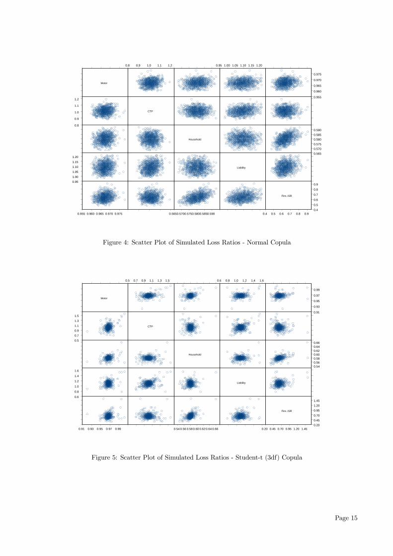
4.1.2 Student-t Copula (3 df)

Compared to the Normal copula case, Figure 5 lacksthe overall linearity in the pair-wise associations be-cause the Student-t copula also captures other formsof dependence as we have noted earlier. For the ma-jority of the pairs, the observations are scattered ran-domly around the centre of the distribution. How-ever in this case, we observe stronger evidence of taildependence especially in the upper tail of the distrib-ution where a large loss for one line results in a simi-larly large loss for the other line. This is expected asthe Student-t copula allows for tail dependence. Seefor example, the pair-wise plots for the motor/CTP(20%) and CTP/liability (25%) business lines.

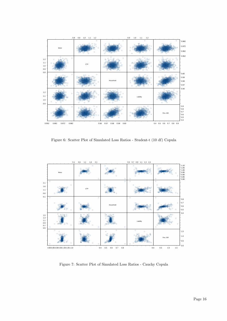
4.1.3 Student-t Copula (10 df)

Although also generated from a Student-t copula, theobservations in Figure 6 appears more akin to the

Page 14

Motor

0.8

0.9

1.0

1.1

1.2

0.951.001.051.101.151.20

0.955 0.960 0.965 0.970 0.975

0.8 0.9 1.0 1.1 1.2

CTP

Household

0.5650.5700.5750.5800.5850.590

0.95 1.00 1.05 1.10 1.15 1.20

Liability

0.955

0.960

0.965

0.970

0.975

0.5650.5700.5750.5800.5850.590

Fire..ISR

0.40.5

0.60.7

0.8

0.9

0.4 0.5 0.6 0.7 0.8 0.9

Figure 4: Scatter Plot of Simulated Loss Ratios - Normal Copula

Motor

0.50.70.91.11.31.5

0.6

0.8

1.0

1.2

1.4

1.6

0.91 0.93 0.95 0.97 0.99

0.5 0.7 0.9 1.1 1.3 1.5

CTP

Household

0.54 0.56 0.580.60 0.620.64 0.66

0.6 0.8 1.0 1.2 1.4 1.6

Liability

0.91

0.93

0.95

0.97

0.99

0.540.560.580.600.620.640.66

Fire..ISR

0.200.450.700.951.201.45

0.20 0.45 0.70 0.95 1.20 1.45

Figure 5: Scatter Plot of Simulated Loss Ratios - Student-t (3df) Copula

Page 15

Motor

0.8

0.9

1.0

1.1

1.2

0.9

1.0

1.1

1.2

0.952 0.962 0.972 0.982

0.8 0.9 1.0 1.1 1.2

CTP

Household

0.56 0.57 0.58 0.59 0.60

0.9 1.0 1.1 1.2

Liability

0.952

0.962

0.972

0.982

0.56

0.57

0.58

0.59

0.60

Fire..ISR

0.40.50.60.70.80.9

0.4 0.5 0.6 0.7 0.8 0.9

Figure 6: Scatter Plot of Simulated Loss Ratios - Student-t (10 df) Copula

Motor

0.1

0.6

1.1

1.6

2.1

0.50.70.91.11.31.5

0.800.850.90 0.95 1.00 1.051.10

0.1 0.6 1.1 1.6 2.1

CTP

Household

0.4 0.5 0.6 0.7 0.8

0.5 0.7 0.9 1.1 1.3 1.5

Liability

0.800.850.900.951.001.051.10

0.4

0.5

0.6

0.7

0.8

Fire..ISR

0.0

0.5

1.0

1.5

0.0 0.5 1.0 1.5

Figure 7: Scatter Plot of Simulated Loss Ratios - Cauchy Copula

Page 16

Motor

0.85

0.95

1.05

1.15

0.9

1.0

1.1

1.2

0.955 0.960 0.965 0.970 0.975

0.85 0.95 1.05 1.15

CTP

Household

0.562 0.572 0.582 0.592

0.9 1.0 1.1 1.2

Liability

0.955

0.960

0.965

0.970

0.975

0.562

0.572

0.582

0.592

Fire..ISR

0.40.5

0.6

0.7

0.80.9

0.4 0.5 0.6 0.7 0.8 0.9

Figure 8: Scatter Plot of Simulated Loss Ratios - Independence Copula

Normal case than the previous Student-t case withmore evidence of linear dependence for some pairs ofbusiness lines. This is attributable to the asymptoticbehaviour of the Student-t copula, again as we notedearlier, that as the degree of freedom becomes large,the copula behaves more like that of a Normal copula.Therefore, although 10 degrees of freedom is not quitelarge enough for strict asymptotic behaviour, but it islarger than the 3 degrees of freedom, and we can stillreasonably justify its similarity to the Normal case.

4.1.4 Cauchy Copula

Now inspecting Figure 7 for the Cauchy copula, itbecomes more difficult to see the presence of the lin-ear dependence between the losses from the differ-ent business lines. Other forms of dependencies arebeing captured in the Cauchy copula including pos-sible strong dependence on the tails. For example,the household/fire & ISR losses appear to capture aquadratic dependence structure, one where it wouldnot have been possible to capture using a Normalcopula alone. Again as expected for this type of cop-ula, there is stronger visual evidence of tail dependen-cies with many more pairs of simultaneously extremevalue observations produced than those by the otherforms of copulas.

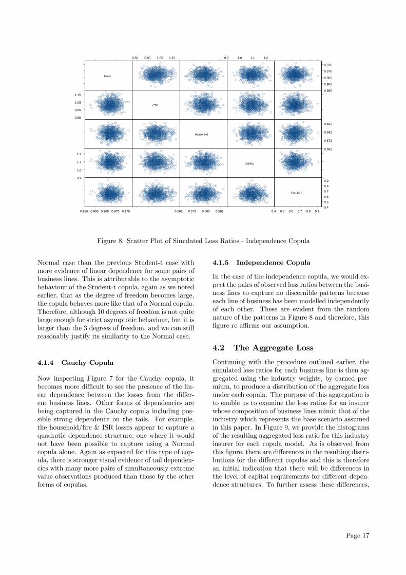
4.1.5 Independence Copula

In the case of the independence copula, we would ex-pect the pairs of observed loss ratios between the busi-ness lines to capture no discernible patterns becauseeach line of business has been modelled independentlyof each other. These are evident from the randomnature of the patterns in Figure 8 and therefore, thisfigure re-affirms our assumption.

4.2 The Aggregate Loss

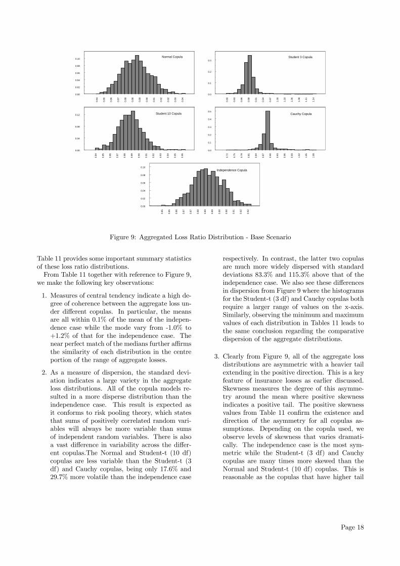
Continuing with the procedure outlined earlier, thesimulated loss ratios for each business line is then ag-gregated using the industry weights, by earned pre-mium, to produce a distribution of the aggregate lossunder each copula. The purpose of this aggregation isto enable us to examine the loss ratios for an insurerwhose composition of business lines mimic that of theindustry which represents the base scenario assumedin this paper. In Figure 9, we provide the histogramsof the resulting aggregated loss ratio for this industryinsurer for each copula model. As is observed fromthis figure, there are differences in the resulting distri-butions for the different copulas and this is thereforean initial indication that there will be differences inthe level of capital requirements for different depen-dence structures. To further assess these differences,

Page 17

0.84

0.85

0.86

0.87

0.88

0.88

0.89

0.90

0.91

0.92

0.92

0.93

0.94

Normal Copula

0.00

0.02

0.04

0.06

0.08

0.10

0.80

0.83

0.86

0.88

0.91

0.94

0.97

1.00

1.03

1.06

1.08

1.11

1.14

Student 3 Copula

0.0

0.1

0.2

0.3

0.84

0.85

0.86

0.87

0.88

0.89

0.90

0.91

0.92

0.93

0.94

0.95

0.96

Student 10 Copula

0.00

0.04

0.08

0.12

0.72

0.75

0.78

0.81

0.84

0.87

0.90

0.93

0.96

0.99

1.02

1.05

1.08

Cauchy Copula

0.0

0.1

0.2

0.3

0.4

0.5

0.85

0.85

0.86

0.87

0.87

0.88

0.89

0.89

0.90

0.90

0.91

0.92

0.92

Independence Copula

0.00

0.02

0.04

0.06

0.08

0.10

Figure 9: Aggregated Loss Ratio Distribution - Base Scenario

Table 11 provides some important summary statisticsof these loss ratio distributions.From Table 11 together with reference to Figure 9,

we make the following key observations:

1. Measures of central tendency indicate a high de-gree of coherence between the aggregate loss un-der different copulas. In particular, the meansare all within 0.1% of the mean of the indepen-dence case while the mode vary from -1.0% to+1.2% of that for the independence case. Thenear perfect match of the medians further affirmsthe similarity of each distribution in the centreportion of the range of aggregate losses.

2. As a measure of dispersion, the standard devi-ation indicates a large variety in the aggregateloss distributions. All of the copula models re-sulted in a more disperse distribution than theindependence case. This result is expected asit conforms to risk pooling theory, which statesthat sums of positively correlated random vari-ables will always be more variable than sumsof independent random variables. There is alsoa vast difference in variability across the differ-ent copulas.The Normal and Student-t (10 df)copulas are less variable than the Student-t (3df) and Cauchy copulas, being only 17.6% and29.7% more volatile than the independence case

respectively. In contrast, the latter two copulasare much more widely dispersed with standarddeviations 83.3% and 115.3% above that of theindependence case. We also see these differencesin dispersion from Figure 9 where the histogramsfor the Student-t (3 df) and Cauchy copulas bothrequire a larger range of values on the x-axis.Similarly, observing the minimum and maximumvalues of each distribution in Tables 11 leads tothe same conclusion regarding the comparativedispersion of the aggregate distributions.

3. Clearly from Figure 9, all of the aggregate lossdistributions are asymmetric with a heavier tailextending in the positive direction. This is a keyfeature of insurance losses as earlier discussed.Skewness measures the degree of this asymme-try around the mean where positive skewnessindicates a positive tail. The positive skewnessvalues from Table 11 confirm the existence anddirection of the asymmetry for all copulas as-sumptions. Depending on the copula used, weobserve levels of skewness that varies dramati-cally. The independence case is the most sym-metric while the Student-t (3 df) and Cauchycopulas are many times more skewed than theNormal and Student-t (10 df) copulas. This isreasonable as the copulas that have higher tail

Page 18

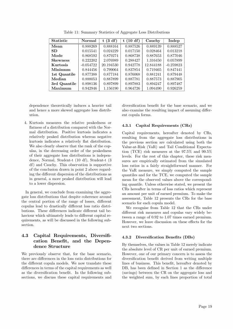
Table 11: Summary Statistics of Aggregate Loss Distributions

Statistic Normal t (3 df) t (10 df) Cauchy IndepMean 0.888269 0.888164 0.887526 0.889139 0.888527SD 0.015541 0.024229 0.017150 0.028464 0.013218Mode 0.868592 0.879274 0.868738 0.887653 0.877046Skewness 0.222202 2.076989 0.288427 1.316450 0.057899Kurtosis -0.054722 20.194530 0.942778 12.844188 -0.259823Minimum 0.844456 0.799064 0.837854 0.719465 0.8474411st Quantile 0.877388 0.877184 0.876068 0.881241 0.879448Median 0.888053 0.887899 0.887781 0.887573 0.8879053rd Quantile 0.898136 0.897899 0.897883 0.894247 0.897487Maximum 0.942946 1.156190 0.964726 1.094490 0.926259

dependence theoretically induces a heavier tailand hence a more skewed aggregate loss distrib-ution.

4. Kurtosis measures the relative peakedness orflatness of a distribution compared with the Nor-mal distribution. Positive kurtosis indicates arelatively peaked distribution whereas negativekurtosis indicates a relatively flat distribution.We also clearly observe that the rank of the cop-ulas, in the decreasing order of the peakednessof their aggregate loss distributions is indepen-dence, Normal, Student-t (10 df), Student-t (3df) and Cauchy. This observation is supportiveof the conclusion drawn in point 2 above regard-ing the different dispersion of the distributions asin general, a more peaked distribution will leadto a lower dispersion.

In general, we conclude from examining the aggre-gate loss distributions that despite coherence aroundthe central portion of the range of losses, differentcopulas lead to drastically different loss ratio distri-butions. These differences indicate different tail be-haviour which ultimately leads to different capital re-quirements, as will be discussed in the following sub-section.

4.3 Capital Requirements, Diversifi-cation Benefit, and the Depen-dence Structure

We previously observe that, for the base scenario,there are differences in the loss ratio distributions forthe different copula models. We now translate thesedifferences in terms of the capital requirements as wellas the diversification benefit. In the following sub-sections, we discuss these capital requirements and

diversification benefit for the base scenario, and wealso examine the resulting impact of assuming differ-ent copula forms.

4.3.1 Capital Requirements (CRs)

Capital requirements, hereafter denoted by CRs,resulting from the aggregate loss distributions inthe previous section are calculated using both theValue-at-Risk (VaR) and Tail Conditional Expecta-tion (TCE) risk measures at the 97.5% and 99.5%levels. For the rest of this chapter, these risk mea-sures are empirically estimated from the simulatedloss ratios in a fairly straightforward manner. Forthe VaR measure, we simply computed the samplequantiles and for the TCE, we computed the samplemean for the observed values above the correspond-ing quantile. Unless otherwise stated, we present theCRs hereafter in terms of loss ratios which representan amount per unit of earned premium. To make theassessment, Table 12 presents the CRs for the basescenario for each copula model.We recognise from Table 12 that the CRs under

different risk measures and copulas vary widely be-tween a range of 0.92 to 1.07 times earned premium.However, we leave discussion on these effects for thenext two sections.

4.3.2 Diversification Benefits (DBs)

By themselves, the values in Table 12 merely indicatethe absolute level of CR per unit of earned premium.However, one of our primary concern is to assess thediversification benefit derived from writing multiplelines of business. This benefit, hereafter denoted byDB, has been defined in Section 1 as the difference(savings) between the CR on the aggregate loss andthe weighted sum, by each lines proportion of total

Page 19

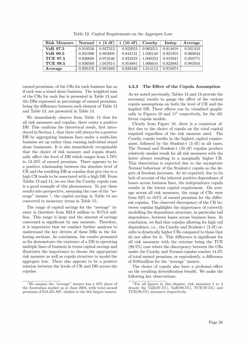
Table 12: Capital Requirements on the Aggregate Loss

Risk Measure Normal t (3 df) t (10 df) Cauchy Indep AverageVaR 97.5 0.919556 0.937313 0.922053 0.963311 0.914818 0.931410VaR 99.5 0.931090 0.982005 0.943131 1.026140 0.921855 0.960844TCE 97.5 0.926698 0.974546 0.933319 1.000353 0.918941 0.950771TCE 99.5 0.936560 1.047614 0.954881 1.066644 0.923883 0.985916Average 0.928476 0.985369 0.938346 1.014112 0.919874

earned premiums, of the CRs for each business line asif each was a stand alone business. The weighted sumof the CRs for each line is presented in Table 13 andthe DBs expressed as percentage of earned premium,being the difference between each element of Table 12and Table 13, are presented in Table 14.

We immediately observe from Table 14 that forall risk measures and copulas, there exists a positiveDB. This confirms the theoretical result, first intro-duced in Section 1, that there will always be a positiveDB by aggregating business lines under a multi-linebusiness set up rather than running individual standalone businesses. It is also immediately recognisablethat the choice of risk measure and copula drasti-cally affect the level of DB which ranges from 1.78%to 13.16% of earned premium. There appears to bea positive relationship between the absolute level ofCR and the resulting DB as copulas that give rise to ahigh CR tends to be associated with a high DB. FromTables 13 and 14, we see that the Cauchy copula caseis a good example of this phenomenon. To put theseresults into perspective, assuming the case of the “av-erage” insurer 1, the capital savings in Table 14 areconverted to monetary terms in Table 15.

The range of capital savings for the “average” in-surer is therefore from $23.8 million to $175.6 mil-lion. This range is large and the amount of savingsconcerned is significant by any measure. Therefore,it is imperative that we conduct further analyses tounderstand the key drivers of these DBs in the fol-lowing sections. In conclusion, the results presentedso far demonstrate the existence of a DB in operatingmultiple lines of business in terms capital savings andillustrates the importance to choose the appropriaterisk measure as well as copula structure to model theaggregate loss. There also appears to be a positiverelation between the levels of CR and DB across thecopulas.

1We assume the “average” insurer has a 10% share ofthe Australian market as at June 2002, with total earnedpremium of $13,351,897, similar to the 6th largest insurer.

4.3.3 The Effect of the Copula Assumption

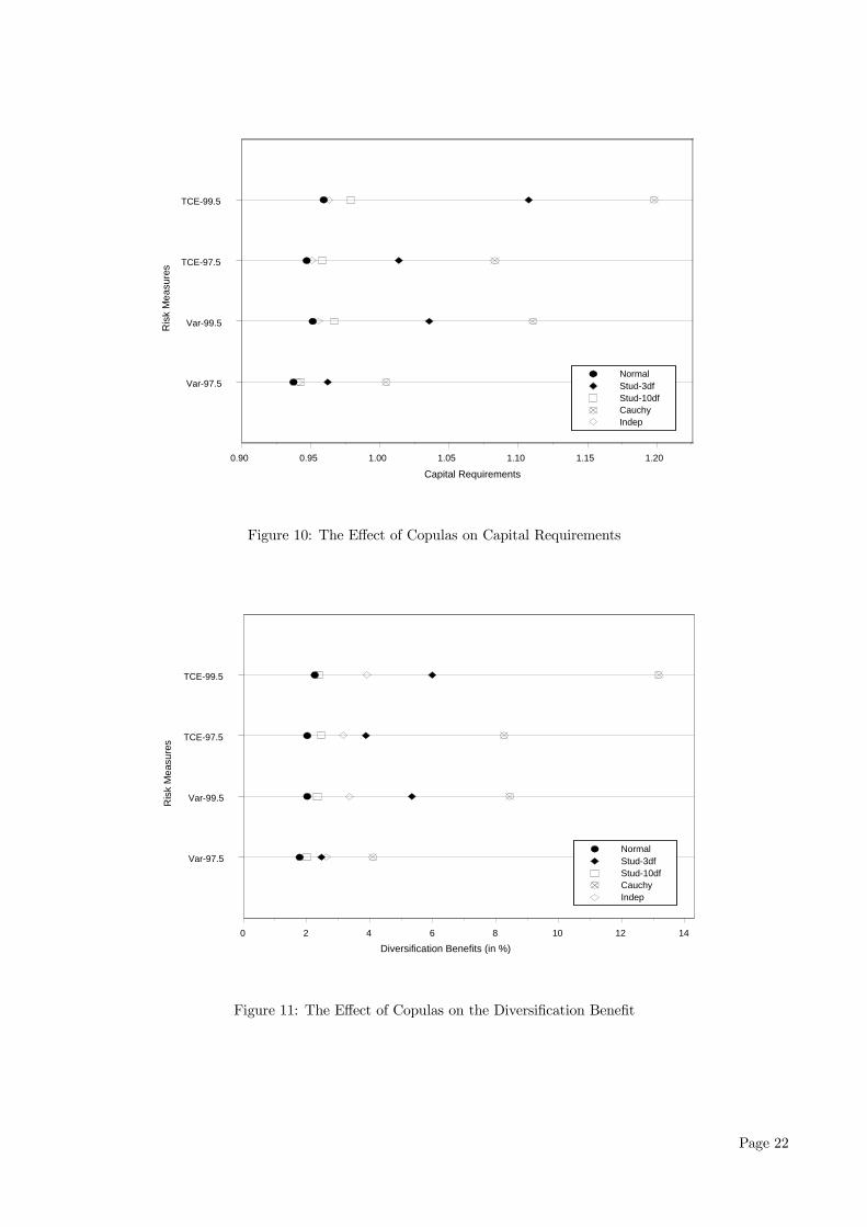
As we noted previously, Tables 12 and 14 provide thenecessary results to gauge the effect of the variouscopula assumptions on both the level of CR and theimplied DB. These effects can be visualised graphi-cally in Figures 10 and 112 respectively, for the dif-ferent copula models.Clearly from Figure 10, there is a consistent ef-

fect due to the choice of copula on the total capitalrequired regardless of the risk measure used. TheCauchy copula results in the highest capital require-ment, followed by the Student-t (3 df) in all cases.The Normal and Student-t (10 df) copulas producerelatively similar result for all risk measures with thelatter always resulting in a marginally higher CR.This observation is expected due to the asymptoticNormal behaviour of the Student-t copula as the de-gree of freedom increases. As we expected, due to itslack of account of the inherent positive dependence oflosses across business lines, the independence copularesults in the lowest capital requirement. On aver-age across all risk measures, the range of CRs werefrom 92% to 101% of earned premium for the differ-ent copulas. The observed discrepency of the CR be-tween copulas highlights the importance of correctlymodelling the dependence structure, in particular taildependence, between losses across business lines. Inconclusion, we find that copulas allowing for high taildependence, i.e., the Cauchy and Student-t (3 df) re-sults in drastically higher CRs compared to those thatdo not allow for it. This difference is significant forall risk measures with the extreme being the TCE(99.5%) case where the discrepency between the CRsunder the Cauchy and Normal copulas reaches 14.3%of total earned premium, or equivalently, a differenceof $191million for the “average” insurer.The choice of copula also have a profound effect

on the resulting diversification benefit. We make thefollowing key observations:

2For all figures in this chapter, risk measures 1 to 4denote the VaR(97.5%), VaR(99.5%), TCE(97.5%) andTCE(99.5%) measures respectively.

Page 20

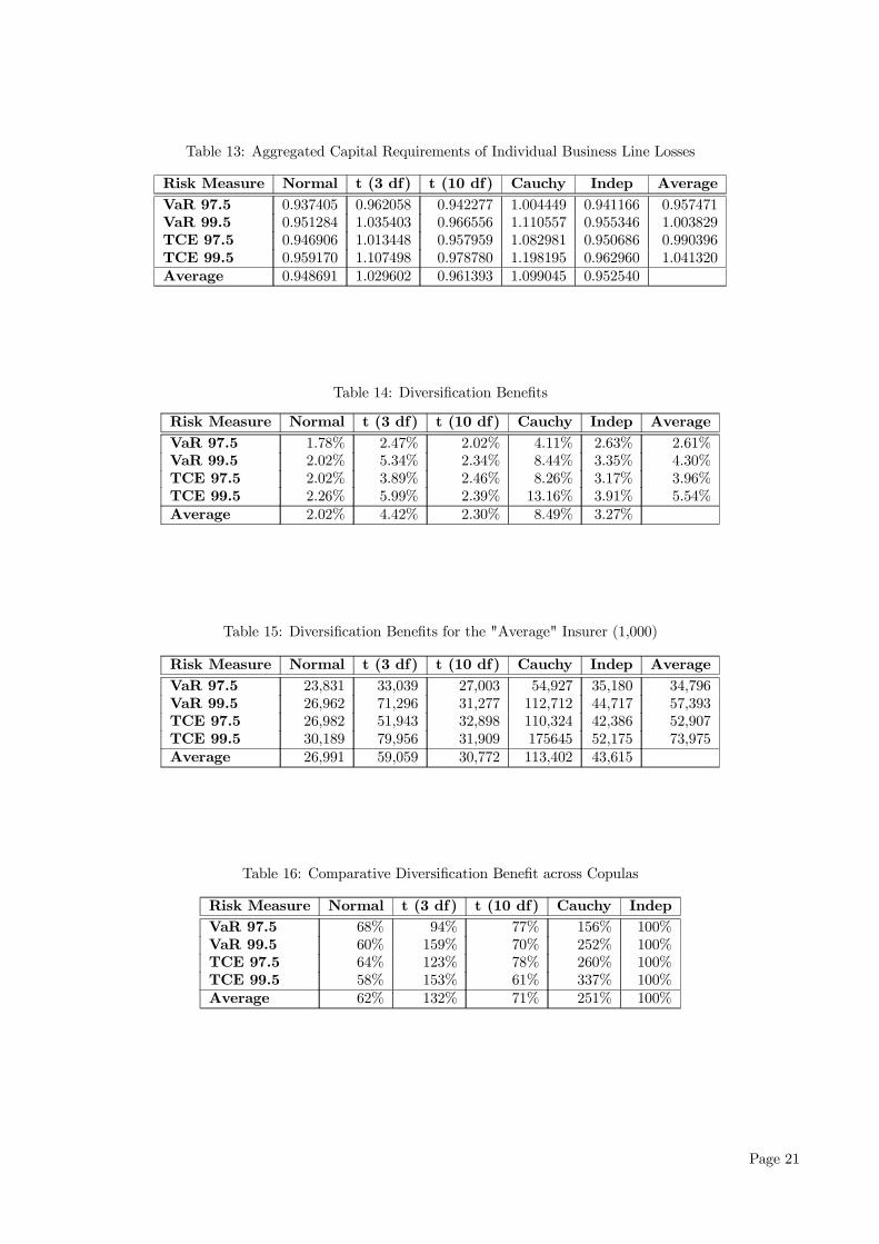
Table 13: Aggregated Capital Requirements of Individual Business Line Losses

Risk Measure Normal t (3 df) t (10 df) Cauchy Indep AverageVaR 97.5 0.937405 0.962058 0.942277 1.004449 0.941166 0.957471VaR 99.5 0.951284 1.035403 0.966556 1.110557 0.955346 1.003829TCE 97.5 0.946906 1.013448 0.957959 1.082981 0.950686 0.990396TCE 99.5 0.959170 1.107498 0.978780 1.198195 0.962960 1.041320Average 0.948691 1.029602 0.961393 1.099045 0.952540

Table 14: Diversification Benefits

Risk Measure Normal t (3 df) t (10 df) Cauchy Indep AverageVaR 97.5 1.78% 2.47% 2.02% 4.11% 2.63% 2.61%VaR 99.5 2.02% 5.34% 2.34% 8.44% 3.35% 4.30%TCE 97.5 2.02% 3.89% 2.46% 8.26% 3.17% 3.96%TCE 99.5 2.26% 5.99% 2.39% 13.16% 3.91% 5.54%Average 2.02% 4.42% 2.30% 8.49% 3.27%

Table 15: Diversification Benefits for the "Average" Insurer (1,000)

Risk Measure Normal t (3 df) t (10 df) Cauchy Indep AverageVaR 97.5 23,831 33,039 27,003 54,927 35,180 34,796VaR 99.5 26,962 71,296 31,277 112,712 44,717 57,393TCE 97.5 26,982 51,943 32,898 110,324 42,386 52,907TCE 99.5 30,189 79,956 31,909 175645 52,175 73,975Average 26,991 59,059 30,772 113,402 43,615

Table 16: Comparative Diversification Benefit across Copulas

Risk Measure Normal t (3 df) t (10 df) Cauchy IndepVaR 97.5 68% 94% 77% 156% 100%VaR 99.5 60% 159% 70% 252% 100%TCE 97.5 64% 123% 78% 260% 100%TCE 99.5 58% 153% 61% 337% 100%Average 62% 132% 71% 251% 100%

Page 21

0.90 0.95 1.00 1.05 1.10 1.15 1.20

Var-97.5

Var-99.5

TCE-97.5

TCE-99.5

NormalStud-3dfStud-10dfCauchyIndep

Capital Requirements

Ris

k M

easu

res

Figure 10: The Effect of Copulas on Capital Requirements

0 2 4 6 8 10 12 14

Var-97.5

Var-99.5

TCE-97.5

TCE-99.5

NormalStud-3dfStud-10dfCauchyIndep

Diversification Benefits (in %)

Ris

k M

easu

res

Figure 11: The Effect of Copulas on the Diversification Benefit

Page 22

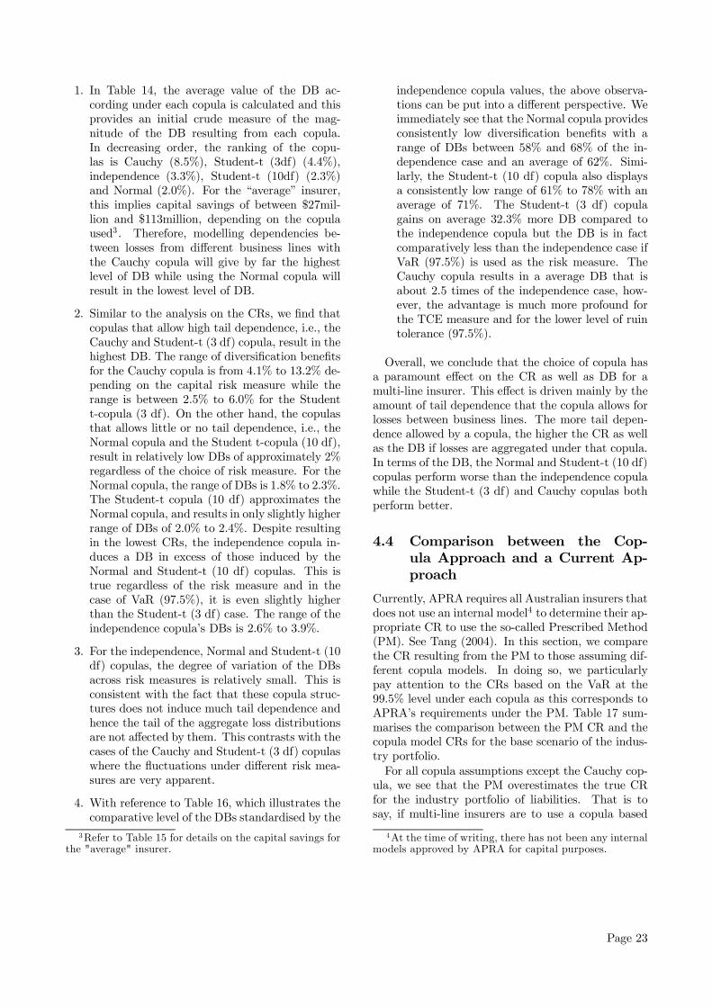
1. In Table 14, the average value of the DB ac-cording under each copula is calculated and thisprovides an initial crude measure of the mag-nitude of the DB resulting from each copula.In decreasing order, the ranking of the copu-las is Cauchy (8.5%), Student-t (3df) (4.4%),independence (3.3%), Student-t (10df) (2.3%)and Normal (2.0%). For the “average” insurer,this implies capital savings of between $27mil-lion and $113million, depending on the copulaused3. Therefore, modelling dependencies be-tween losses from different business lines withthe Cauchy copula will give by far the highestlevel of DB while using the Normal copula willresult in the lowest level of DB.

2. Similar to the analysis on the CRs, we find thatcopulas that allow high tail dependence, i.e., theCauchy and Student-t (3 df) copula, result in thehighest DB. The range of diversification benefitsfor the Cauchy copula is from 4.1% to 13.2% de-pending on the capital risk measure while therange is between 2.5% to 6.0% for the Studentt-copula (3 df). On the other hand, the copulasthat allows little or no tail dependence, i.e., theNormal copula and the Student t-copula (10 df),result in relatively low DBs of approximately 2%regardless of the choice of risk measure. For theNormal copula, the range of DBs is 1.8% to 2.3%.The Student-t copula (10 df) approximates theNormal copula, and results in only slightly higherrange of DBs of 2.0% to 2.4%. Despite resultingin the lowest CRs, the independence copula in-duces a DB in excess of those induced by theNormal and Student-t (10 df) copulas. This istrue regardless of the risk measure and in thecase of VaR (97.5%), it is even slightly higherthan the Student-t (3 df) case. The range of theindependence copula’s DBs is 2.6% to 3.9%.

3. For the independence, Normal and Student-t (10df) copulas, the degree of variation of the DBsacross risk measures is relatively small. This isconsistent with the fact that these copula struc-tures does not induce much tail dependence andhence the tail of the aggregate loss distributionsare not affected by them. This contrasts with thecases of the Cauchy and Student-t (3 df) copulaswhere the fluctuations under different risk mea-sures are very apparent.

4. With reference to Table 16, which illustrates thecomparative level of the DBs standardised by the

3Refer to Table 15 for details on the capital savings forthe "average" insurer.

independence copula values, the above observa-tions can be put into a different perspective. Weimmediately see that the Normal copula providesconsistently low diversification benefits with arange of DBs between 58% and 68% of the in-dependence case and an average of 62%. Simi-larly, the Student-t (10 df) copula also displaysa consistently low range of 61% to 78% with anaverage of 71%. The Student-t (3 df) copulagains on average 32.3% more DB compared tothe independence copula but the DB is in factcomparatively less than the independence case ifVaR (97.5%) is used as the risk measure. TheCauchy copula results in a average DB that isabout 2.5 times of the independence case, how-ever, the advantage is much more profound forthe TCE measure and for the lower level of ruintolerance (97.5%).

Overall, we conclude that the choice of copula hasa paramount effect on the CR as well as DB for amulti-line insurer. This effect is driven mainly by theamount of tail dependence that the copula allows forlosses between business lines. The more tail depen-dence allowed by a copula, the higher the CR as wellas the DB if losses are aggregated under that copula.In terms of the DB, the Normal and Student-t (10 df)copulas perform worse than the independence copulawhile the Student-t (3 df) and Cauchy copulas bothperform better.

4.4 Comparison between the Cop-ula Approach and a Current Ap-proach

Currently, APRA requires all Australian insurers thatdoes not use an internal model4 to determine their ap-propriate CR to use the so-called Prescribed Method(PM). See Tang (2004). In this section, we comparethe CR resulting from the PM to those assuming dif-ferent copula models. In doing so, we particularlypay attention to the CRs based on the VaR at the99.5% level under each copula as this corresponds toAPRA’s requirements under the PM. Table 17 sum-marises the comparison between the PM CR and thecopula model CRs for the base scenario of the indus-try portfolio.For all copula assumptions except the Cauchy cop-

ula, we see that the PM overestimates the true CRfor the industry portfolio of liabilities. That is tosay, if multi-line insurers are to use a copula based

4At the time of writing, there has not been any internalmodels approved by APRA for capital purposes.

Page 23

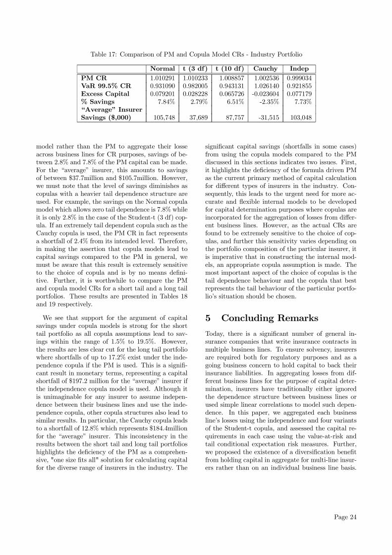
Table 17: Comparison of PM and Copula Model CRs - Industry Portfolio

Normal t (3 df) t (10 df) Cauchy IndepPM CR 1.010291 1.010233 1.008857 1.002536 0.999034VaR 99.5% CR 0.931090 0.982005 0.943131 1.026140 0.921855Excess Capital 0.079201 0.028228 0.065726 -0.023604 0.077179% Savings 7.84% 2.79% 6.51% -2.35% 7.73%“Average” InsurerSavings ($,000) 105,748 37,689 87,757 -31,515 103,048

model rather than the PM to aggregate their losseacross business lines for CR purposes, savings of be-tween 2.8% and 7.8% of the PM capital can be made.For the “average” insurer, this amounts to savingsof between $37.7million and $105.7million. However,we must note that the level of savings diminishes ascopulas with a heavier tail dependence structure areused. For example, the savings on the Normal copulamodel which allows zero tail dependence is 7.8% whileit is only 2.8% in the case of the Student-t (3 df) cop-ula. If an extremely tail dependent copula such as theCauchy copula is used, the PM CR in fact representsa shortfall of 2.4% from its intended level. Therefore,in making the assertion that copula models lead tocapital savings compared to the PM in general, wemust be aware that this result is extremely sensitiveto the choice of copula and is by no means defini-tive. Further, it is worthwhile to compare the PMand copula model CRs for a short tail and a long tailportfolios. These results are presented in Tables 18and 19 respectively.

We see that support for the argument of capitalsavings under copula models is strong for the shorttail portfolio as all copula assumptions lead to sav-ings within the range of 1.5% to 19.5%. However,the results are less clear cut for the long tail portfoliowhere shortfalls of up to 17.2% exist under the inde-pendence copula if the PM is used. This is a signifi-cant result in monetary terms, representing a capitalshortfall of $197.2 million for the “average” insurer ifthe independence copula model is used. Although itis unimaginable for any insurer to assume indepen-dence between their business lines and use the inde-pendence copula, other copula structures also lead tosimilar results. In particular, the Cauchy copula leadsto a shortfall of 12.8% which represents $184.4millionfor the “average” insurer. This inconsistency in theresults between the short tail and long tail portfolioshighlights the deficiency of the PM as a comprehen-sive, "one size fits all" solution for calculating capitalfor the diverse range of insurers in the industry. The

significant capital savings (shortfalls in some cases)from using the copula models compared to the PMdiscussed in this sections indicates two issues. First,it highlights the deficiency of the formula driven PMas the current primary method of capital calculationfor different types of insurers in the industry. Con-sequently, this leads to the urgent need for more ac-curate and flexible internal models to be developedfor capital determination purposes where copulas areincorporated for the aggregation of losses from differ-ent business lines. However, as the actual CRs arefound to be extremely sensitive to the choice of cop-ulas, and further this sensitivity varies depending onthe portfolio composition of the particular insurer, itis imperative that in constructing the internal mod-els, an appropriate copula assumption is made. Themost important aspect of the choice of copulas is thetail dependence behaviour and the copula that bestrepresents the tail behaviour of the particular portfo-lio’s situation should be chosen.

5 Concluding Remarks

Today, there is a significant number of general in-surance companies that write insurance contracts inmultiple business lines. To ensure solvency, insurersare required both for regulatory purposes and as agoing business concern to hold capital to back theirinsurance liabilities. In aggregating losses from dif-ferent business lines for the purpose of capital deter-mination, insurers have traditionally either ignoredthe dependence structure between business lines orused simple linear correlations to model such depen-dence. In this paper, we aggregated each businessline’s losses using the independence and four variantsof the Student-t copula, and assessed the capital re-quirements in each case using the value-at-risk andtail conditional expectation risk measures. Further,we proposed the existence of a diversification benefitfrom holding capital in aggregate for multi-line insur-ers rather than on an individual business line basis.

Page 24

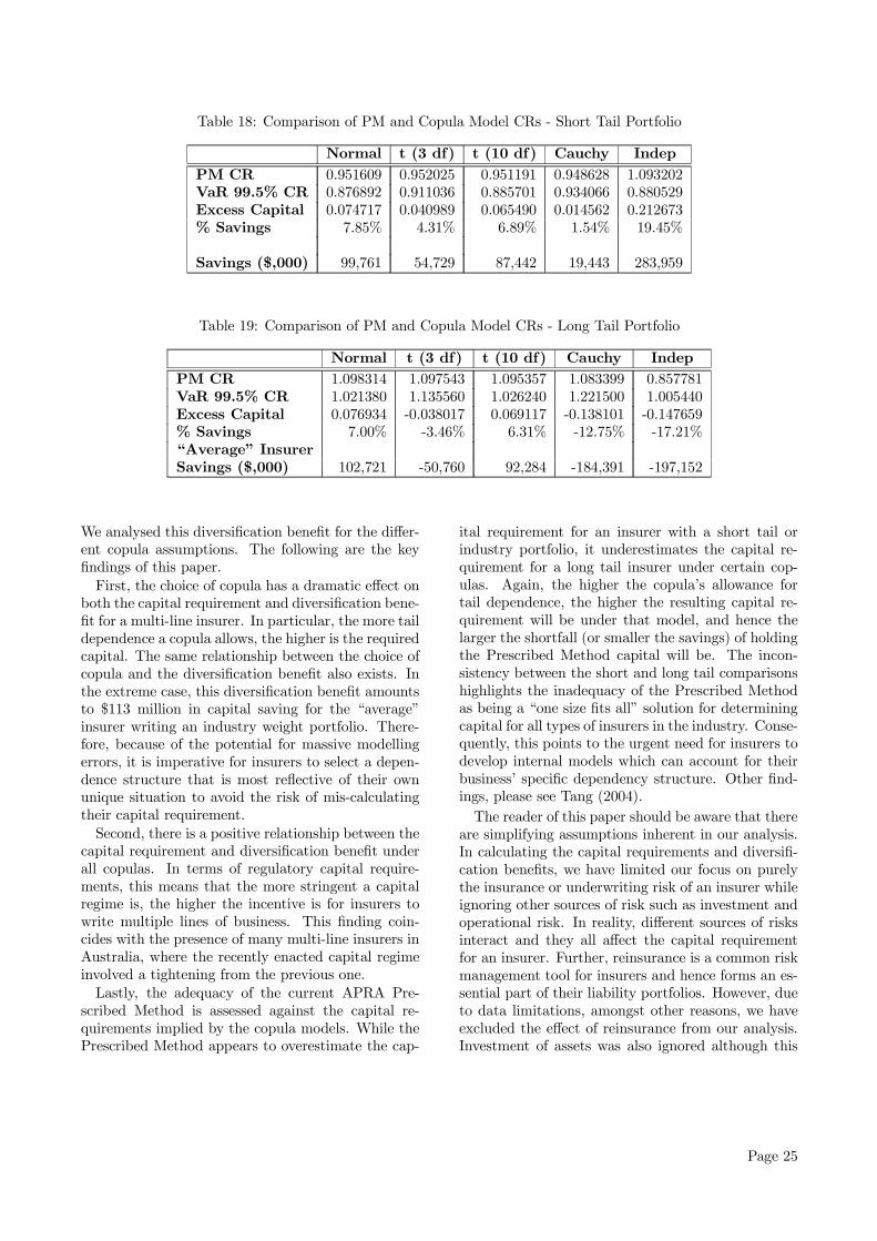
Table 18: Comparison of PM and Copula Model CRs - Short Tail Portfolio

Normal t (3 df) t (10 df) Cauchy IndepPM CR 0.951609 0.952025 0.951191 0.948628 1.093202VaR 99.5% CR 0.876892 0.911036 0.885701 0.934066 0.880529Excess Capital 0.074717 0.040989 0.065490 0.014562 0.212673% Savings 7.85% 4.31% 6.89% 1.54% 19.45%

Savings ($,000) 99,761 54,729 87,442 19,443 283,959

Table 19: Comparison of PM and Copula Model CRs - Long Tail Portfolio

Normal t (3 df) t (10 df) Cauchy IndepPM CR 1.098314 1.097543 1.095357 1.083399 0.857781VaR 99.5% CR 1.021380 1.135560 1.026240 1.221500 1.005440Excess Capital 0.076934 -0.038017 0.069117 -0.138101 -0.147659% Savings 7.00% -3.46% 6.31% -12.75% -17.21%“Average” InsurerSavings ($,000) 102,721 -50,760 92,284 -184,391 -197,152

We analysed this diversification benefit for the differ-ent copula assumptions. The following are the keyfindings of this paper.First, the choice of copula has a dramatic effect on

both the capital requirement and diversification bene-fit for a multi-line insurer. In particular, the more taildependence a copula allows, the higher is the requiredcapital. The same relationship between the choice ofcopula and the diversification benefit also exists. Inthe extreme case, this diversification benefit amountsto $113 million in capital saving for the “average”insurer writing an industry weight portfolio. There-fore, because of the potential for massive modellingerrors, it is imperative for insurers to select a depen-dence structure that is most reflective of their ownunique situation to avoid the risk of mis-calculatingtheir capital requirement.Second, there is a positive relationship between the

capital requirement and diversification benefit underall copulas. In terms of regulatory capital require-ments, this means that the more stringent a capitalregime is, the higher the incentive is for insurers towrite multiple lines of business. This finding coin-cides with the presence of many multi-line insurers inAustralia, where the recently enacted capital regimeinvolved a tightening from the previous one.Lastly, the adequacy of the current APRA Pre-

scribed Method is assessed against the capital re-quirements implied by the copula models. While thePrescribed Method appears to overestimate the cap-

ital requirement for an insurer with a short tail orindustry portfolio, it underestimates the capital re-quirement for a long tail insurer under certain cop-ulas. Again, the higher the copula’s allowance fortail dependence, the higher the resulting capital re-quirement will be under that model, and hence thelarger the shortfall (or smaller the savings) of holdingthe Prescribed Method capital will be. The incon-sistency between the short and long tail comparisonshighlights the inadequacy of the Prescribed Methodas being a “one size fits all” solution for determiningcapital for all types of insurers in the industry. Conse-quently, this points to the urgent need for insurers todevelop internal models which can account for theirbusiness’ specific dependency structure. Other find-ings, please see Tang (2004).The reader of this paper should be aware that there

are simplifying assumptions inherent in our analysis.In calculating the capital requirements and diversifi-cation benefits, we have limited our focus on purelythe insurance or underwriting risk of an insurer whileignoring other sources of risk such as investment andoperational risk. In reality, different sources of risksinteract and they all affect the capital requirementfor an insurer. Further, reinsurance is a common riskmanagement tool for insurers and hence forms an es-sential part of their liability portfolios. However, dueto data limitations, amongst other reasons, we haveexcluded the effect of reinsurance from our analysis.Investment of assets was also ignored although this

Page 25

would have only had a minor effect due to the shortterm nature of general insurers’ investments.Due to these assumptions, the single most signif-

icant limitation to the results of this paper is thatthey merely serve to compare the effect of the depen-dence structure on the capital requirements and doesnot quantify the required capital that a particular in-surer should hold. In particular, the results cannotbe directly compared with other studies that considerthe total capital requirement for an insurer. The cap-ital requirements calculated in this paper is not rep-resentative beyond the amount of assets required toensure a specific level of confidence in meeting its in-surance losses within a one year period. The numeri-cal results in monetary terms presented in this papermust also be taken with caution as this is only rep-resentative of the “average” insurer as defined in thispaper and again, we emphasise that it only accountsfor the insurance risk component of the total capitalrequirements. However, the modelling procedure ofaggregating risks using copulas as demonstrated inthis paper can be readily adapted.Given that our findings in this paper indicate a

pronounced effect of the copula structure on the cap-ital requirements for insurers, we suggest further re-search into using other copulas to model the depen-dence structure of multi-line insurers’ portfolios. Inthis paper, we have explored using elliptical copu-las to model the dependence structure but these areonly a few of the vast pool of copula structures thatone can draw from. Isaacs (2003) explored the sameaggregation process using the Gumbel copula, a rep-resentative of heavy tail dependence copulas whichappear to be very suitable for capital determinationpurposes. However, the specification of a Gumbelcopula only involves pair-wise associations and henceis not appropriate for application to multi-line insur-ers with more than two business lines.We can also apply copula approaches to model

other risk dependencies in the general insurers’ busi-ness. For example, rather than modelling the depen-dency at the business line level, one may investigatedependencies between risk sources such as those be-tween investment and operational risks.Catastrophes that affect multiple lines of business

are often modelled as a separate class in a dynamicmodel. To this end, we may find interesting results ifthe analysis of this paper was performed on a portfoliowith a separate catastrophe business line.Furthermore, we can relax some of our assumptions

in our modelling to alleviate some of the limitationspreviously mentioned. For example, we can performthe analysis on a net rather than gross basis so thatreinsurance effects on the capital requirements are al-

lowed for. Another suggestion is to factor in expensesand possibly the effects of investments as these alsoinfluence capital requirements. Sensitivities of thecapital requirement under the copula models to thesize of the insurer and the correlation matrix assump-tion can also be explored.

References

[1] APRA (2002) “General Insurance PrudentialStandards and Guidance Notes 110 and 210,”Australian Prudential Regulatory Authority.

[2] APRA (1996 - 2002) "Selected Statistics on theGeneral Insurance Industry, December 1996 -June 2002" Australian Prudential RegulatoryAuthority.

[3] Artzner, P., Delbaen, F., Eber, J.M., and Heath,D. (1999) “Coherent Measures of Risk,” Mathe-matical Finance 9: 203-228.

[4] Basel Committee on Banking Supervision (2004)"International Convergence of Capital Measure-ment and Capital Standards, a Revised Frame-work," Bank for International Settlements.

[5] Bateup, R. and Reed, I. (2001) “Researchand Data Analysis Relevant to the Develop-ment of Standards and Guidelines on Liabil-ity Valuation for General Insurance,” paper pre-pared for the Institute of Actuaries of Australiaand APRA, Tillinghast Towers-Perrin. Availablefrom <www.actuaries.asn.au>

[6] Brender, A. (2002) “The Use of Internal Mod-els for Determining Liabilities and Capital Re-quirements,” North American Actuarial Journal6: 1-10.

[7] Butsic, R.P. (1994) “Solvency Measurement forProperty-Liability Risk-Based Capital Applica-tions,” Journal of Risk and Insurance 61(4): 656-690.

[8] Carriere, J.F. (2003) “Copulas,” working paper,University of Alberta, Canada.

[9] CIBC (2004) “Investor Relations BreakfastSeries - Economic Capital & Asset Liabil-ity Management,” presentation slides, Cana-dian Imperial Bank of Commerce. Available at<www.cibc.ca>

Page 26

[10] Collings, S. and White, G. (2001) “APRA RiskMargin Analysis,” paper presented at the Insti-tute of Actuaries of Australia XIIIth General In-surance Seminar, Trowbridge Consulting. Avail-able from <www.actuaries.asn.au>

[11] Creedon, S., Chalk, A., Chaplin, M., Goodchild,J., Jones, T., Postlewhite, S., Powls, G., Shel-don, T., Tuley, J., Webber, J. and Wilson, C.(2003) “Risk and Capital Assessment and Super-vision in Financial Firms,” interim working partyreport, prepared for the Finance and InvestmentConference of the UK actuarial profession.

[12] Daykin, C.D., Bernstein, G.D., Couttes, S.M.,Devitt, E.R.F., Hey, G.B., Reynolds, D.I.W. andSmith, P.D. (1987) “Assessing the Solvency andFinancial Strength of a General Insurance Com-pany,” Journal of the Institute of Actuaries, 114:227-325.

[13] Dhaene, J., Denuit, M., Goovaerts, M., Kaas,R., and Vyncke, D. (2002a) “The Concept ofComonotonicity in Actuarial Science and Fi-nance: Theory,” Insurance: Mathematics & Eco-nomics 31: 3-33.

[14] Dhaene, J., Denuit, M., Goovaerts, M., Kaas,R., and Vyncke, D. (2002b) “The Concept ofComonotonicity in Actuarial Science and Fi-nance: Applications,” Insurance: Mathematics& Economics 31: 133-161.

[15] Dhaene, J., Goovaerts, M.J., and Kaas, R.(2003) “Economic Capital Allocation Derivedfrom Risk Measures,” North American ActuarialJournal 7: 44-59.

[16] Embrechts, P., Lindskog, F., and McNeil,A. (2001) “Modelling Dependence with Cop-ulas and Applications to Risk Management,”working paper, ETHZ, Zurich. Available at<www.math.ethz.ch/finance>.

[17] Embrechts, P., McNeil, A., and Straumann, D.(1999) “Correlation and Dependence in RiskManagement: Properties and Pitfalls,” RiskManagement: Value at Risk and Beyond, ed.by Dempster, M. and Moffatt, H.K., CambridgeUniversity Press.

[18] European Commision (2004), “Solvency II,”note to the IC solvency subcommittee, EuropeanCommission Internal Markets DG.

[19] Fang, K.T., Kotz, S. and Ng, K.W. (1987) Sym-metric Multivariate and Related DistributionsLondon: Chapman & Hall.

[20] Feller, W. (1966) An Introduction to ProbabilityTheory and its Applications - Volume II NewYork, NY: John Wiley & Sons.

[21] Frank, M. (1979) “On the Simultaneous Associa-tivity of F (x, y) and x + y − F (x, y),” Aequa-tiones Mathematicae 19: 194-226.

[22] Frechet, M. (1951) “Sur les tableaux de correla-tion dont les marges sont donnees,” Ann. Univ.Lyon, Sci., 14: 53-77.

[23] Frechet, M. (1957) “Les tableaux de correlationdont les marges et des bornes sont donnees,”Ann. Univ. Lyon, Sci., 20: 13-31.

[24] Frees, E.W. and Valdez, E.A. (1998) “Under-standing Relationships Using Copulas,” NorthAmerican Actuarial Journal 2: 1-25.

[25] Genest, C. (1987) “Frank’s Family of BivariateDistributions,” Biometrika 74: 549-555.

[26] Genest, C. and MacKay, J. (1986a) “The Joy ofCopulas: Bivariate Distributions with UniformMarginals,” The American Statistician 40: 280-283.

[27] Giese, G. (2003) “Economic Capital versus Reg-ulatory Capital - A Market Benchmark,” RiskMay 2003. Available from <www.risk.net>.

[28] Goovaerts, M., DeVijlder, F. and Haezen-donck, J. (1984) Insurance Premiums Amster-dam: North Holland Publishers.

[29] Gray, B. (2001) “Prudential Supervi-sion of General Insurance - Policy Dis-cussion Paper,” APRA. Available from<http://www.apra.gov.au>.

[30] Hart, D.G., Buchanan, R.A. and Howe, B.A.(1996) The Actuarial Practice of General Insur-ance Sydney: Institute of Actuaries of Australia.

[31] IAA Insurance Regulation Committee (2002)“Report of Solvency Working Party,” Inter-national Actuarial Association. Available from<www.actuaries.org>.

[32] IAA Solvency Assessment Working Party (2004)“A Global Framework for Insurer Solvency As-sessment,” International Actuarial Association.Available from <www.actuaries.org>.

[33] Isaacs, D. (2003) “Capital Adequacy and De-pendence,” paper presented at the Institute ofActuaries of Australia XIVth General InsuranceSeminar.

Page 27

[34] Joe, H. (1997) Multivariate Models and Depen-dence Concepts London: Chapman & Hall.

[35] Juri, A. and Wüthrich, M.V. (2002) “CopulaConvergence Theorems for Tail Events,” Insur-ance: Mathematics & Economics 30: 405-420.

[36] Kaas, R., Goovaerts, M., Dhaene, J. and De-nuit, M. (2001) Modern Actuarial Risk TheoryNetherlands: Kluwer Academic Publishers.

[37] Klugman, S.A., Panjer, H.H., Willmot, G.E.,(1998) Loss Models - From Data to DecisionsDanvers, MA: John Wiley & Sons.

[38] Landsman, Z. and Valdez, E.A. (2003) “TailConditional Expectations for Elliptical Distrib-utions,” North American Actuarial Journal, toappear.

[39] Mueller, H. (2004) “Economic Capital - Re-cent Market Developments and Current Trends,”SoA topics in actuarial analysis series, Fi-nancial Engineering NewsTM. Available from<www.fenews.com>.

[40] Nelsen, R. (1999) An Introduction to CopulasNew York, NY: Springer.

[41] Office of the Insurance Commissioner (1992 -1996) "Selected Statistics on the General Insur-ance Industry — Total Industry In and Outsideof Australia, December 1992 - June 1996", Officeof the Insurance Commissioner.

[42] Panjer, H.H. (2002) “Measurement of Risk, Sol-vency Requirements, and Allocation of Capitalwithin Financial Conglomerates,” Institute of In-surance and Pension Research, University of Wa-terloo, Research Report 01-14.

[43] Priest, C. (2003) “Correlations: What TheyMean - And More Importantly What They Don’tMean,” paper presented at the 2003 Institute ofActuaries Australia Biennial Convention.

[44] Sherris, M. and Sutherland-Wong, C. (2004)“Risk-Based Regulatory Capital for Insurers: ACase Study,” paper presented at the 14th AnnualAFIR Colloquium, Boston, U.S.A. Availablefrom <http://www.actuarial.unsw.edu.au>.

[45] Sklar, A. (1959) “Fonctions de repartition à ndimensions et leurs marges,” Pub. Inst. Statist.Univ. Paris 8: 229-231.

[46] Sutherland-Wong, C. (2003) “A Comparison ofMethods for APRA’s General Insurance CapitalRequirements,” University of New South Wales.

[47] Tang, A. (2004) “Economic Capital and the Ag-gregation of Risks Using Copulas,” Honours the-sis, Actuarial Studies, University of New SouthWales.

[48] Valdez, E.A. (2003) “Modelling Dependencewith Copulas in Insurance and Finance,” pre-sentation KVBA-ARAB, Brussels, Belgium.

[49] Valdez, E.A. and Chernih, A. (2003) “Wang’sCapital Allocation Formula for Elliptically Con-toured Distributions,” Insurance: Mathematics& Economics 33: 517-532.

[50] Vanduffel, S. (2004) “Comonotonicity: FromRisk Measurement to Risk Management,” PhDthesis, Katholieke Universiteit-Leuven, Belgium.

A Generating MultivariateRandom Vectors

The purpose of this appendix is to show how one cango about generating random vectors. One of the use-ful applications of copulas is the resulting ease of gen-erating random vectors. One procedure is describedin Nelsen (1999), by considering the conditional dis-tribution

c (v |u ) = Prob (V ≤ v |U = u)

= lim∆u→0

C (u+∆u, v)−C (u, v)

∆u=

∂

∂uC (u, v)

then the following generates (u, v) pairs:

1. generate two independent U (0, 1), denote themby u and t;

2. set v = c(−1) (t |u), the quasi-inverse of c (t |u) ;

3. (u, v) is the desired pair with uniform marginalsand copula C.

Recall that the copula defined by

C (u1, ..., un) = H¡Φ−1 (u1) , ...,Φ

−1 (un)¢

is called the Normal copula. The following algorithmgenerates (x1, x2, ..., xn) from the normal copula:

1. Construct the lower triangular matrix B so thatthe covariance matrix V = BBT using Choleski’sdecomposition;

2. Generate a column vector of independentstandard normal random variables Z =(Z1, Z2, ..., Zn)

T ;

Page 28

3. Take the matrix product of B and Z, i.e. Y =BZ;

4. Set Ui = Φ (Yi) for i = 1, 2, ..., n;

5. Set Xi = F−1Xi(Ui) for i = 1, 2, ..., n.

6. (x1, x2, ..., xn) is the desired vector with mar-ginals FX1 , ..., FXn and normal copula C.

Recall that the copula defined by

Tυ (z1, ..., zn) =

Z zn

−∞

Z zn−1

−∞· · ·Z z1

−∞fν (x1, ..., xn) dx1 · · · dxn

is called the t copula. The following algorithm gen-erates (x1, x2, ..., xn) from the t copula:

1. Construct the lower triangular matrix B so thatthe covariance matrix V = BBT using Choleski’sdecomposition;

2. Generate a column vector of independentstandard normal random variables Z =(Z1, Z2, ..., Zn)

T ;

3. Take the matrix product of B and Z, i.e. Y =BZ;

4. Generate a chi-squared random variable S ∼χ2 (ν) with ν degrees of freedom, independentof Z;

5. Set Ti =p

υSYi for i = 1, 2, ..., n;

6. Set Ui = tυ (Ti) for i = 1, 2, ..., n;

7. Set Xi = F−1Xi(Ui) for i = 1, 2, ..., n.

8. (x1, x2, ..., xn) is the desired vector with mar-ginals FX1 , ..., FXn and t copula C.

To generate from a Cauchy copula, we simply setthe degrees of freedom to be υ = 1 and followed theabove procedure for simulating random vectors froma Student-t copula. We will need the above simula-tion procedures to simulate claim values with differ-ent copulas. Programs written in SAS and Splus.

Page 29