Policy Research Working Paper 6530

Economic Development As Opportunity Equalization

John E. Roemer

The World BankDevelopment Economics Vice PresidencyPartnerships, Capacity Building UnitJuly 2013

WPS6530P

ublic

Dis

clos

ure

Aut

horiz

edP

ublic

Dis

clos

ure

Aut

horiz

edP

ublic

Dis

clos

ure

Aut

horiz

edP

ublic

Dis

clos

ure

Aut

horiz

edP

ublic

Dis

clos

ure

Aut

horiz

edP

ublic

Dis

clos

ure

Aut

horiz

edP

ublic

Dis

clos

ure

Aut

horiz

edP

ublic

Dis

clos

ure

Aut

horiz

ed

Produced by the Research Support Team

Abstract

The Policy Research Working Paper Series disseminates the findings of work in progress to encourage the exchange of ideas about development issues. An objective of the series is to get the findings out quickly, even if the presentations are less than fully polished. The papers carry the names of the authors and should be cited accordingly. The findings, interpretations, and conclusions expressed in this paper are entirely those of the authors. They do not necessarily represent the views of the International Bank for Reconstruction and Development/World Bank and its affiliated organizations, or those of the Executive Directors of the World Bank or the governments they represent.

Policy Research Working Paper 6530

Economic development should be conceived of as the degree to which an economy has implemented an efficient and just distribution of economic resources. The ubiquitous measure of GDP per capita reflects a utilitarian conception of justice, where individual utility is defined as personal income, and social welfare is the average of utilities in a population. A more attractive conception of justice is opportunity-equalization. Here, a two-dimensional measure of economic development is proposed, based upon viewing individuals’ incomes as

This paper is a product of the Partnerships, Capacity Building Unit, Development Economics Vice Presidency. It is part of a larger effort by the World Bank to provide open access to its research and make a contribution to development policy discussions around the world. Policy Research Working Papers are also posted on the Web at http://econ.worldbank.org. The author may be contacted at john.roemer@yale.edu.

a consequence of circumstances, effort, and policy. The first dimension is the average income level of those in the society with the most disadvantaged circumstances, and the second dimension is the degree to which total income inequality is due to differential effort, as opposed to differential circumstances. This pair of numbers is computed for a set of 22 European countries. No country dominates all others on both dimensions. The two-dimensional measure induces a partial ordering of countries with respect to development.

“Economic development as opportunity equalization”

by

John E. Roemer*

Yale University

Key words: economic development, equality of opportunity

JEL categories: O1, D3, D63

Sector Board: Economic Policy (EPOL) and Poverty Reduction (POV)

* John Roemer is a professor of political science and economics at Yale University; his e-mail address is john.roemer@yale.edu I am grateful to referees of this journal for suggestions leading to important revisions, and to the many scholars with whom I have discussed these ideas. This article is based upon a lecture given at the ABCDE meeting in Paris, 2011.

2

1. Introduction1

Suppose we are concerned with the inequalities that exist in a society with respect

to the distribution of some desirable good or advantage – wealth, life expectancy,

literacy, or wage-earning capacity. The causes of inequality in that distribution can be

partitioned into two categories: those for which individuals should not be held

responsible, and those for which they should be. We need not here be concerned with

the problem of free will, and the possibility that people are not responsible for anything if

they lack free will, because every society has a conception of responsibility, and we may

take that as the politically salient conception. Thus, in many societies, it is thought

wrong that an individual’s income be strongly correlated with her parent’s education or

social position, for, assuming that that correlation reflects causality, these family

characteristics seem to be ones from which children should not differentially benefit or

suffer. On the other hand, most societies believe that adults should be held responsible

for various choices that they make, assuming that they possess adequate information

about the alternatives. Let us call the social and biological aspects of a person’s

environment for which society believes he should not be responsible his circumstances,

those choices and actions for which he should be held responsible, his effort, and the

desirable good whose distribution we are concerned with the objective.

When we have a data set that permits us to measure the inequality in the

distribution of the objective, and its correlation with circumstances and effort, it is

usually necessary (because data sets are finite) to choose a fairly small number of

1 This section reviews previous work of the author on the conceptualization of equality of opportunity (see Roemer (1993, 1998, 2002)).

3

circumstances, each of which can take on a fairly small number of values. Thus, one

circumstance might be parental education, which one could partition into three values;

another might be race, partitioned into three categories, and so on. Call a vector of

circumstances a type. Thus, one may partition the population of the data set into a finite

number of types, where a type is the set of individuals with (approximately) the same

vector of circumstances. Denote the types by Denote the level of the

objective with which we are concerned (income, wage-earning capacity, or life

expectancy) by u, which is a function of circumstances, policy, and effort. Thus,

is the average level of the objective for individuals of type t whose effort choices

are summarized by the vector e if the policy is . Denote the policy space by . In

this formulation, any characteristic of the individual is either a component of

circumstance, or of effort.

Effort here is measured so that increasing effort produces an increasing value of

the objective. In this way, effort’s role in the functions differs from its relationship to

utility in economic theory. For example, if the objective is health status, then refraining

from smoking constitutes positive effort, although that abstinence may lower ‘utility’ in

the usual sense, where the utility function is a representation of subjective preferences.

If the population faces a policy , there will ensue a distribution of effort in

each type; denote the distribution functions of these probability distributions by .

These distribution functions will, of course, have characteristics that reflect type – that is,

circumstances. For instance, we will find different distributions of smoking behavior in

different socio-economic types. Because the goal of equal-opportunity policy is to

compensate persons for their circumstances, we should compensate them as well for the

4

effect of their circumstances on their effort. How can we decide when two persons, of

different types, have expended comparable degrees of effort? I propose to measure the

degree of a person’s effort by his rank in the distribution . Rank sterilizes out of the

distribution aspects of it that reflect circumstances. Thus, for example, if we view ‘years

of education chosen’ as effort, and persons in two different types both rank at the 80th

centile of the distributions of years of education in their respective types, we will declare

them to have expended equal degrees of effort (although their actual years of education

may be quite different).

We may thus define the function

, (1)

which is the (average) value of the objective, when the policy is , of the individuals at

the quantile of the distribution of effort of their type. If effort is uni-dimensional, the

function is well-defined. If e is multi-dimensional, then in general it is not, and we

should then replace vectors of effort with, for example, the linear combination of its

components that best explains the value of the objective. For practical purposes,

however, in many applications, one need never measure effort: one can simply define the

values directly as the level of the objective in type t at the quantile of the

distribution of the objective in that type. Implicitly, this approach assumes that effort is

declared to be that constellation of choices that enhance the value of the objective,

conditional upon type.

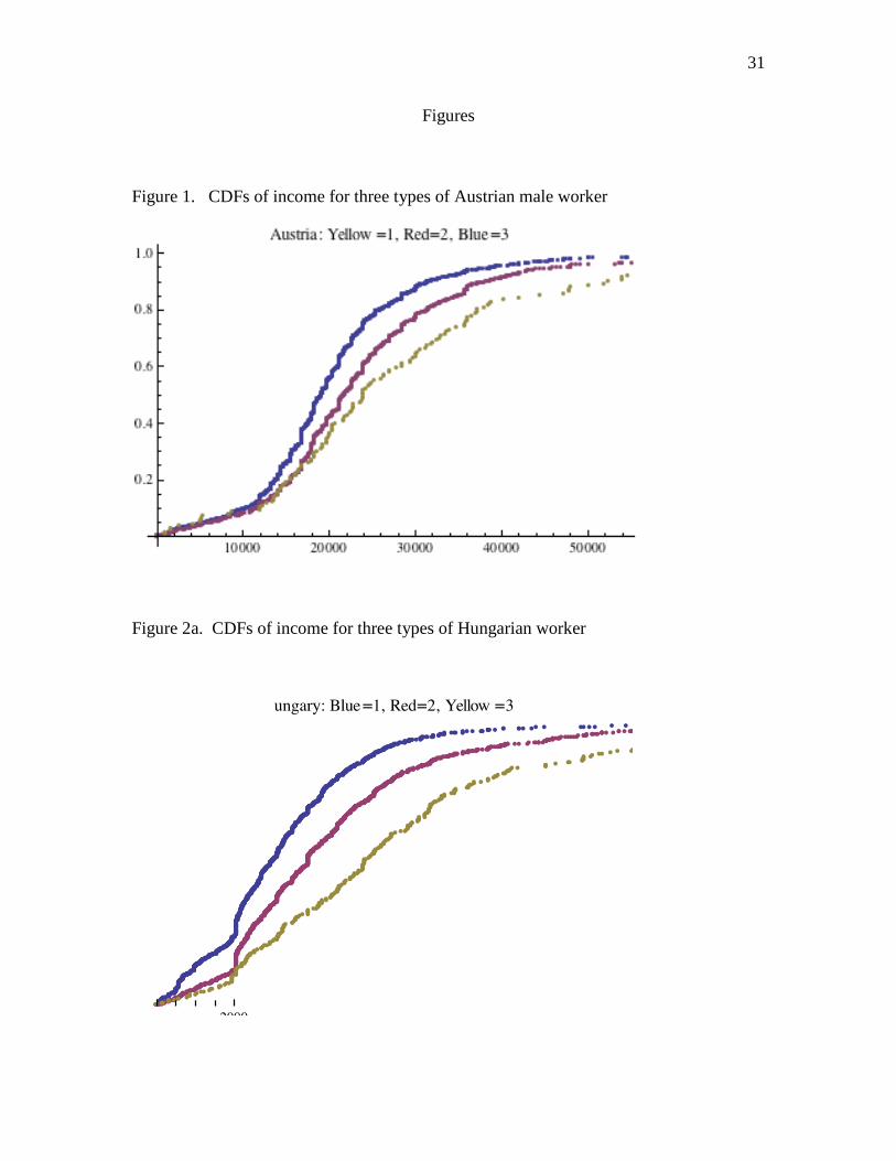
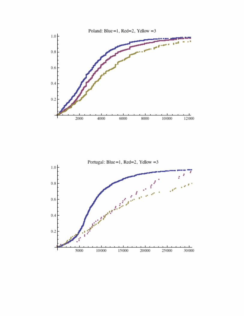
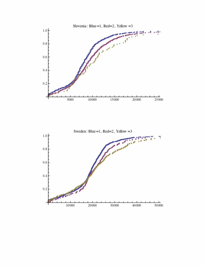
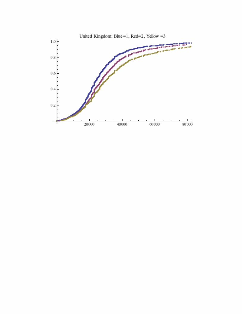
In figure 1, we see the distribution function of post-fisc income of three types of

men in Austria, in 2005, where the unique circumstance defining type is the level of

education of the individual’s more educated parent. The yellow curve is the distribution

5

function of those men whose parent had at least some tertiary education; the red curve, of

those men whose parent had 12 years of education, and the blue curve, of those men

whose parent had less than 12 years of education.

Taking the objective to be post-fisc income, the inverses of the functions in the

graph are the functions . So to see the graphs of the three functions , simply

reflect figure 1 over the vertical axis and then rotate it 90 degrees clockwise.

Holding persons responsible for their effort means that if two individuals in the

same type (who are exposed to identical policy treatments by hypothesis) sustain

different values of the objective, there is no inequity, because by hypothesis, these

different values are due to differential effort, something for which they are responsible.

However, differences between the functions are ethically undesirable – a reflection of

unequal opportunities—because individuals are not responsible for their

type/circumstances. Therefore, the goal of policy should be so render the functions

as similar as possible. Since we identify individuals at the same rank of their

distributions as having expended equal degrees of effort, the goal is to choose the policy

to render the distribution functions (in Figure 1) as close together as they can be (that

is, to minimize the horizontal distance between the functions).

But we do not want equality of distribution functions at a low level: we therefore

desire some kind of maxi-minimization. Suppose we fixed a particular value of ;

inequality in the T numbers is due not to differential effort, by

hypothesis, but to differential circumstances. Thus, we should choose the policy to

. (2)

6

However, we are concerned with every level of effort: a reasonable way of addressing all

effort levels is to take the average of the numbers being maximized in (2), that is, to

choose policy to

. (3)

I call the solution to (3) the equal opportunity policy. It must be emphasized that this

policy is conditional upon the definition of circumstances, and the choice of policy

space2.

Define . defines an ordering on ; that is to

say that:

,

In words, is the average value of the lower envelope of the objective functions,

across types.

There is a special case of interest. Typically, there are constraints that we impose

upon policies, so that the policy space for the problem, , is fairly small – for example,

we may limit ourselves to affine income tax policies, a uni-dimensional (small) set in the

large set of income-tax policies. In this case, it may well be that there is one type –

denote it type 1 -- that for all policies is unambiguously the most disadvantaged

one, in the sense that its distribution function is dominated (first-order stochastically) by

the others at every policy. This is virtually the case in figure 1, where the distribution

functions are stacked almost unambiguously – it is obvious that the most disadvantaged

2 A generalization of program (3) is provided in Roemer (2012), where a large family of possible equality-of-opportunity measures is proposed.

7

type is the one of men whose more educated parent had fewer than twelve years of

education, as its income distribution function is virtually FOSD by the distributions of the

other two types3. In this case, the left-hand envelope of the distribution functions is

simply the distribution function of a single type, and equation (3) reduces to:

(4)

where is the average value of the objective4 in the most disadvantaged type under

policy ϕ. In this case, the equal-opportunity ethic directs us to choose the policy to

maximize the average value of the objective in the most disadvantaged type – assuming

that this type is unambiguously the most disadvantaged, for any feasible policy5.

It is worthwhile contrasting the equal-opportunity ethic with one of its main

competitors, the utilitarian ethic. Denote by the fraction of the population in type t.

The utilitarian policy maximizes the ordering given by:

(5)

i.e., the average value of the objective in the population. 3 First-order stochastic dominance does not hold for very low incomes in figure 1; almost surely, this is the case because the children of highly educated parents are going to university, and earning very low incomes early in their careers, less than those who have entered the working-class after secondary school. 4 Recall that the area above a distribution function and bounded by the line at ordinate value one is the mean of the distribution. 5 Indeed, an alternative proposal, due to van de Gaer (1993), is to implement equality of opportunity by maximizing the function . In , the

‘min’ and ‘integral’ operators are commuted, with respect to . Fleurbaey and Peragine (2012) call an ‘ex post’ approach, and an ‘ex ante’ approach to measuring equality of opportunity. In Roemer (2012), I offer reasons for my preference for the measure . However, what the text has just pointed out is that, in special cases, the two measures coincide.

8

A third ordering, associated with John Rawls, is the ordering which maximizes

the minimum value of the objective in the population; I will write:

. (6)

We see that the equal-opportunity ethic lies ‘between’ utilitarianism and the Rawlsian

difference principle; it is less extreme than the Rawlsian formulation, in that it maximizes

an average of minima across effort levels. Actually, my naming of (6) as the Rawlsian

view is not quite fair, for Rawls wrote that the difference principle should apply to ‘social

groups,’ not individuals. If we take the different types to be the relevant social groups,

then, at least in the special case where (4) holds, the equal-opportunity ethic maximizes

the minimum objective value over social groups, and hence possesses a Rawlsian

ancestry.

In the general case, however, if the distribution functions cross, the solution of (3)

does not entail maximizing the average value of the most disadvantaged type, but rather,

maximizing the area above the left-hand envelope of the distribution functions of the

types, and bounded by the horizontal line of height one.

To summarize, we have provided an ordering of policies with respect to the equal-

opportunity ethic. That ordering takes as data a particular social view of personal

responsibility, summarized in a set of circumstances and an implied typology – a partition

of the population – and a policy space. The objective for which opportunities are to be

equalized is typically some measurable and interpersonally comparable kind of

advantage, the kind of thing a ministry in a government might be concerned with, such as

income, health, life expectancy, or educational achievement.

9

2. Economic development

Economic development should be measured by the extent to which a society has

achieved a desirable distribution of advantage. Desirability should include

considerations of both efficiency and justice or fairness. Indeed, the most common

measure of economic development, GDP per capita, is based upon the utilitarian ethic,

which computes the level of social welfare as the average of the utilities in the

population, where utility is taken to be proportional to income.

The human development index (HDI) is not utilitarian, because it is not an

average of a value of some kind of advantage over a population. But it is a convex

combination of the average of three kinds of advantage over a population: the

individual’s income (or consumption), his degree of literacy (which could be coded as 0

or 1), and his life expectancy6. The human development index is an average of the

averages of these three dimensions over the whole society. So the HDI does not

essentially depart from utilitarian practice in that it looks only at population averages,

although it looks at three averages instead of only one. To be precise, this description is

valid for the HDI as defined up to the 2009 Human Development Report of the UNDP.

But in 2010, the Human Development Report introduced the ‘inequality adjusted human

development index,’which, although still consequentialist, is not utilitarian.

Neither of these measures of development is sensitive to the distinction between

circumstances and effort. They are consequentialist measures of how well an economic

system is doing, in that the data required to assess the system’s desirability are the values

6 An individual’s life expectancy can be defined as the average age of death of a cohort of persons with the individual’s characteristics. I am assuming that the life expectancy in a country is the average of life expectancies of individuals, so defined.

10

of various outcomes for members of the population. The equal-opportunity view,

however, focuses upon the distinction between circumstances and effort. Thus, to assess

the desirability of a system, it requires not only the data just mentioned, but also

knowledge of the type of each individual. It is a non-consequentialist measure, for it will

assess differently the same outcome for two individuals, if they have different

circumstances. Utilitarianism condemns inequalities if their elimination would increase

average or total welfare (however it is measured); opportunity egalitarianism condemns

them to the extent they are due to circumstances beyond the control of the individuals

concerned. The views are quite different.

Opportunity egalitarianism is not only a superior ethic to utilitarianism, it is the

one implicitly endorsed by members of many societies. Suppose one asks the proverbial

man on the street, “Do you think that the inequality between the rich Mr. A and poor Ms.

B is unjustified?” it is unlikely that he will answer, “Only if a redistribution from A to B

would increase their total welfare.” But he might well answer, “It depends upon how

hard they each worked.” In other words, the popular views of justice are not

consequentialist, they are based upon notions of desert, and desert is based upon

measurements of effort. Our man on the street must know more than the aggregate

distribution of the objective to assess whether that distribution is fair – he must know the

(disaggregated) distributions of the objective by type. The source of the inequality

matters, ethically speaking, but these sources are ignored by looking only at outcomes7.

7 There is substantial survey and experimental work which examines the views that people in various societies have concerning distributive justice. An extensive discussion of this literature is found in Gaertner and Schokkaert (2012).

11

We cannot maintain that the most common measures of economic development

are value free: they are derived from a utilitarian ethic. To this claim one might object

that the measure of GDP per capita has nothing to do with utilitarianism, it is simply a

proxy for technological development. But this cannot be right, because economists are

not interested in technological prowess per se: we are interested in human welfare. We

would not consider a society highly developed which possessed a fine technology run by

slaves, whose product all went, but for the slaves’ subsistence, to the prince. So an

attempt to justify the GDP per capita measure of development as a value-free measure of

technological accomplishment has the undesirable consequence of obliterating the

distinction between economics and engineering – namely, that economics must always

focus upon human welfare8.

Therefore, we should use the best conception of justice or social welfare to derive

a measure of economic development. Perhaps the extent to which opportunities have

been equalized is not the best such conception, but it dominates, so I believe, utilitarian

measures. It is better to measure the level of economic development by some statistic

that reflects equality of opportunity rather than by a utilitarian measure.

But what version of equality of opportunity should we use to evaluate economic

development in a panel of countries? What should be the circumstances and the

objective? To be most similar to GDP per capita, the objective should be income – let us

say, post-fisc income including the per capita value of public goods. Begin with

circumstances that include the educational level and occupations of the parents of the

8 I do not wish to denigrate the goals of engineers. However, there is a sense in which engineers are interested in technological efficiency as a goal, while economists are interested in it only insofar as technological efficiency is necessary for Pareto efficiency (in which the goal is human welfare).

12

individuals, and the ethnicity and gender of the individual9. Then calculate the number

, where is the status quo policy. This is the first component of the

two-dimensional measure of economic development that I propose. The value is

the average income of those in society who are most disadvantaged by circumstances.

Choosing it as a measure of economic development is inspired by the view, attributed to

Mohandes Ghandi, among many others, that “a nation’s greatness is measured by how it

treats its weakest members.10” This proposal is not new. Indeed Bourguignon, Ferrera

and Walton (2007) propose a dynamic and closely related version of : namely they

say that the present discounted value of the average income of the most disadvantaged

type should be maximized for development policy to be equitable.

3. The degree of opportunity equality

I have proposed to measure the level of development of a society as the value of

the equal-opportunity social welfare function. Of course, we are highly restricted in our

ability to measure economic development when we must use a single number to capture

it. In particular, applying the measure defined in (4) to income does not allow us to

distinguish the wealth of the society from the degree to which the society has succeeded

in eliminating injustice – that being the influence of circumstances upon inequality. To

do this, I propose a second measure, which I call the degree of opportunity equality11.

9 How one treats gender depends upon whether one uses households or the individual as the unit. 10 The quotation is ubiquitously attributed to Ghandi, over the original statement of it is obscure. 11 Again, this proposal is not new. It is a special case of the ‘inequality of opportunity ratio (IOR)’ defined in Ferreira and Gignoux (2011). Ferreira and Gignoux’s preferred measure of inequality is not CV2 but the ‘mean logarithmic deviation.’ The same idea for measuring the degree of inequality due to circumstances is proposed in Checchi and Peragine (2010) as well.

13

A society will have achieved equality of opportunity to the extent that the

contribution of differential circumstances to total inequality in the distribution of the

objective is small. Let the distribution function of the objective in a given society be H,

and the distribution functions of the objectives in the types be ; then

. (7)

Suppose we measure inequality in a distribution by the coefficient of variation squared

(CV2 ), that is:

. (8)

where the mean of H is . Denote the mean of . Without loss of generality,

suppose that we have enumerated types so that is a monotone increasing sequence.

Define the distribution:

, (9)

Clearly the mean of is . If were the actual distribution of the objective in

society, then everybody in a given type would have exactly the same value of the

objective, equal to the mean of the objective in that type. Were this the case, then the

contribution of effort to inequality would be nil, as no variation of accomplishment would

exist within any type. Now it is well-known that we can decompose as follows:

, (10)

14

where . Since both contributions in this decomposition are positive, it is natural

to interpret as the amount of inequality due to circumstances, and

the amount of inequality due to effort. I therefore propose, as a

measure of the degree of opportunity equalization, the index:

. (11)

We may want to think of as an upper bound on the fraction of inequality due to

effort because surely some circumstances have not been taken into account, whose effect

is measured, residually, as ‘effort.’

My suggestion is that we measure economic development by the ordered pair

. Note that neither component of d is a consequentialist measure. One

cannot recover either or η from knowledge of the distribution of income (more

generally, the objective) alone. One must know, as well, the circumstances of

individuals, which capture the concept of responsibility salient for the society in question.

4. Country calculations of the level and degree of development

In this section, I calculate the value of d for a set of OECD countries. The data

upon which these calculations are based are taken from EU-SILC 2005. The sample

consists of male workers, who are partitioned into three types, based upon the maximum

of the worker’s parents’ educational levels:

Type 1: the worker’s more educated parent had at most lower secondary

education

15

Type 2: the worker’s more educated parent had at least upper secondary education

but not tertiary education

Type 3: the worker’s more educated parent had at least some tertiary education.

The net income for each respondent is recorded, which includes earnings, self-

employment income, after taxes and transfers. The single characteristic of type in these

calculations is parental education which takes on three values.12

The fact that income does not include the value of public goods is a weakness of

the measure. If a country has a high rate of taxation, and a substantial fraction of tax

revenues finance public goods (as opposed to transfer payments), this will not be

reflected in the income data. Transfer payments are included in the definition of income.

Figure 1 presents the income-distribution functions for Austria, by type, which is

in many ways typical. Since the left-hand envelope of the three CDFs is, for all practical

purposes, the CDF of type 1, the level of development is simply the mean of type 1’s

income. For Austria, the level and degree of development, as defined in the previous

section, are:

.

(Incomes are measured in Euros.) It may surprise the reader that only about 3% of

income inequality is attributed to circumstances, but this is quite typical for advanced

European countries, given that only one circumstance is specified. For Latin American

12 I am grateful to Daniele Checchi and Francesco Scervini for providing me with the data set. For an exact description of the data set, see Checchi, Peragine, and Serlenga (2010). The computation of the degrees of development and the type-distributions of income were performed by the author using Mathematica; I will supply the code upon request.

16

countries, this number will be considerably larger. Indeed, Ferreira and Gignoux (2011),

in their table 8, present their comparable measure to , using the mean logartithmic

deviation of income as the inequality measure, for a set of six Latin American countries.

Their set of circumstances is denser than mine. For some countries (Guatamala), the

degree of inequality attributable to circumstances is over 50%.

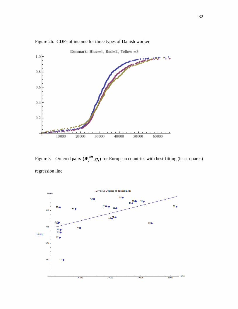
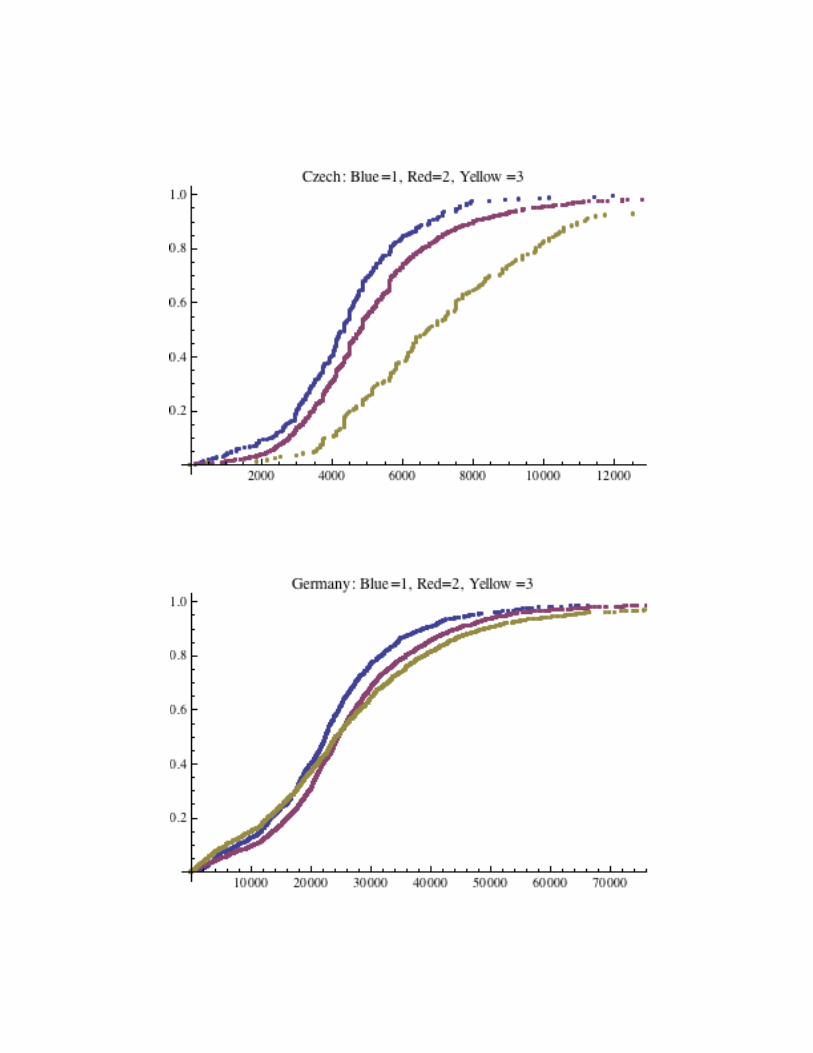
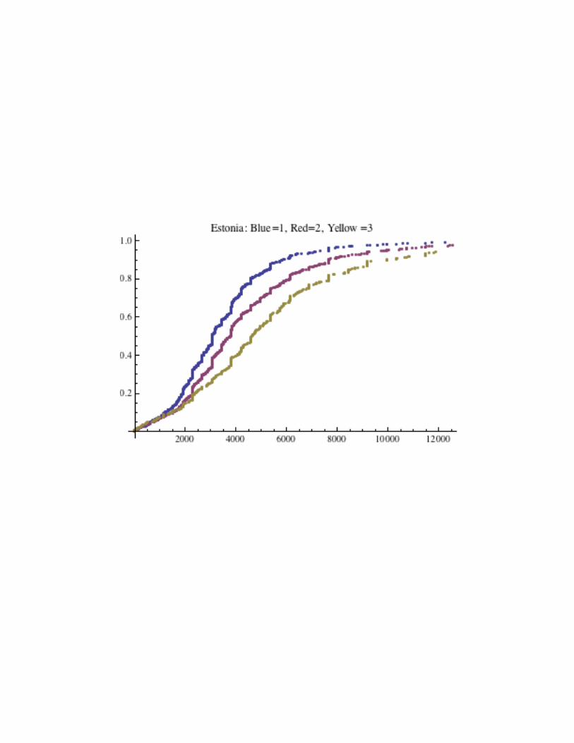
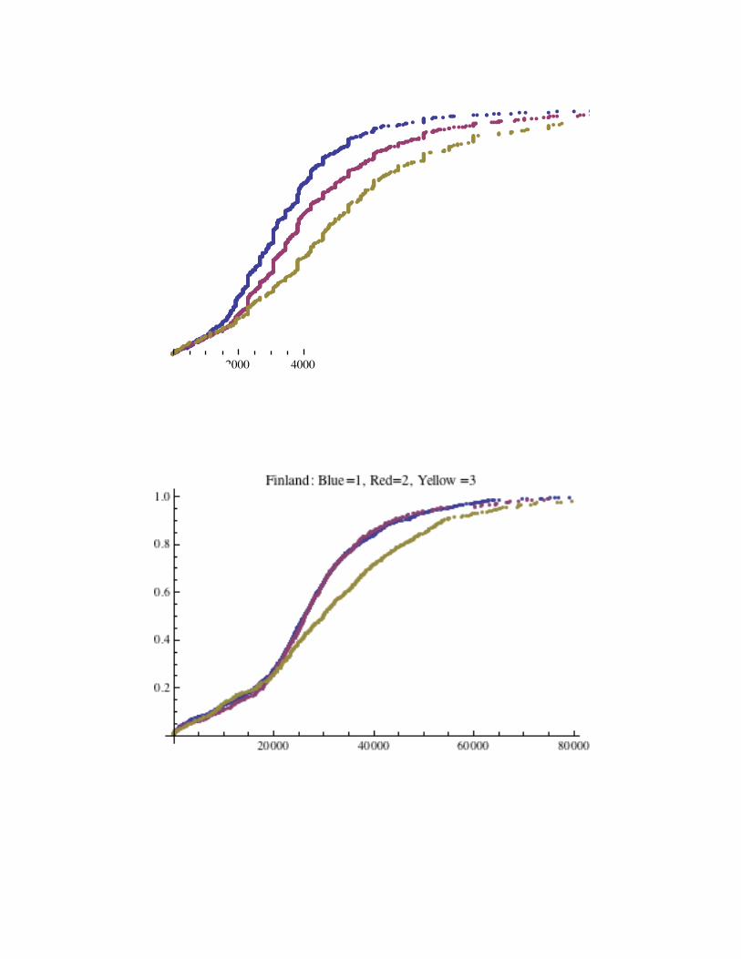
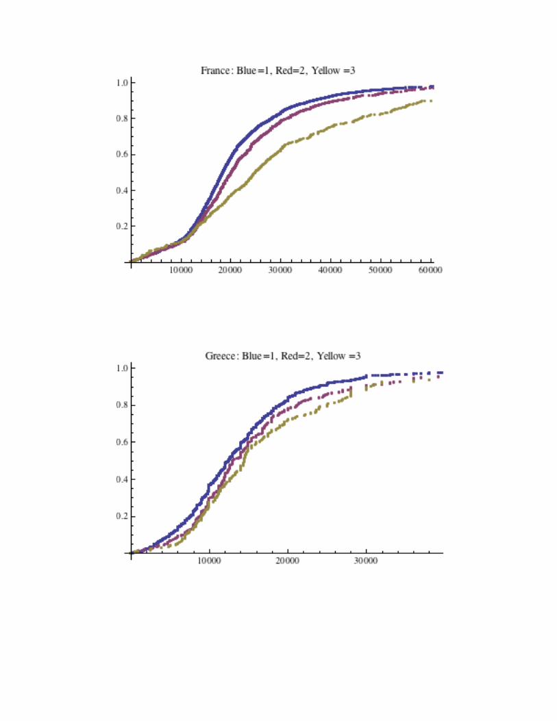
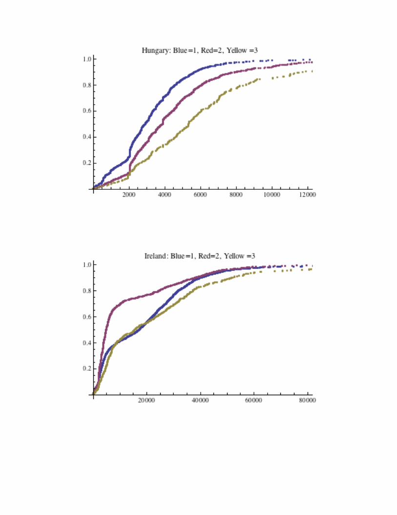
Figure 2 presents the income CDFs of the three types for one of the least

developed countries in sample, Hungary, and for one of the most developed, Denmark.

We see that the inter-type dispersion is considerably more dramatic in Hungary

than in Austria, while the CDFs in Denmark are very close together. The graphs of the

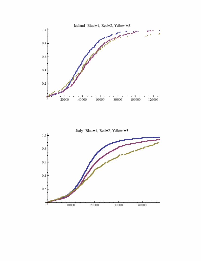
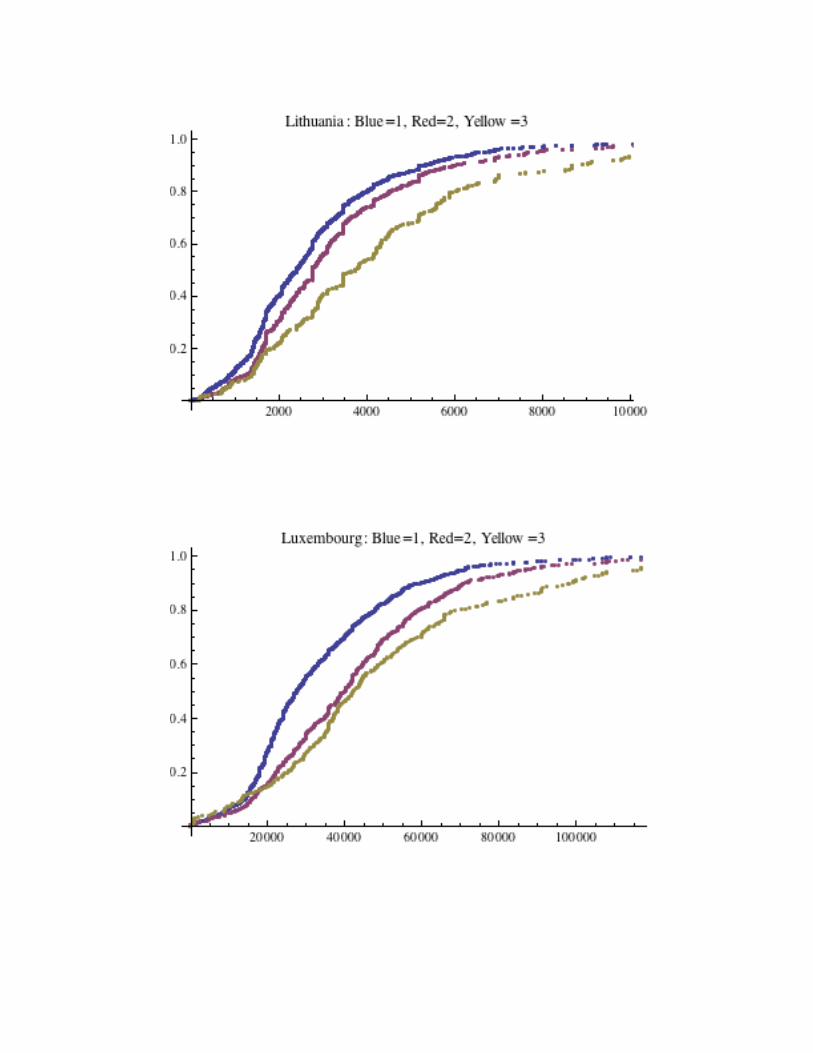
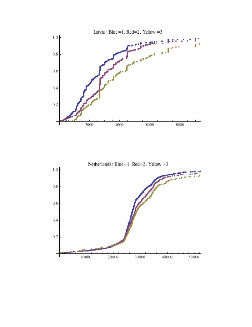
three CDFs for the other countries in the sample are presented in an online appendix.

Figure 3 plots the ordered pairs for all 22 countries in the sample13.

Some comments:

1. The eastern European countries are the worst off with respect to the index : these

comprise Lithuania (LT), Estonia (EE), the Czech Republic(CZ), Poland (PL), Latvia

(LV), and Hungary (HU). (Slovenia (SI) does somewhat better.) But Spain (ES) is also

very low on this measure. With respect to the degree of development, η, the eastern

European countries span a range from about 92% to 99.5% .

2. Greece appears to do very well on the degree of development: I question whether the

data are reliable.

13 EU-SILC also contains data for Cyprus, but there are so few observations that I do not consider the CDFs to be meaningful. I excluded as well Ireland from the sample, because I believe the data have been miscoded: according to the data, the middle type in Ireland is worse off than the most disadvantaged type.

17

3. We may define a partial order with respect to development; a country j dominates a

country k if

.

With regard to this partial order, no country in the sample dominates all others. Thus,

we can say there exists no most developed European country. Conversely, however,

there are five countries that are undominated by any other: Denmark (DK) , Iceland (IS),

Germany (DE), the UK, and the Netherlands (NL). These data are from 2005, and

doubtless Iceland, post-crash, no longer enjoys this status.

Table 1 presents the same data as figure 1.

As noted, Ferreira and Gignoux (2011) calculate a similar statistic to for six

Latin American countries. Their calculation differs from the one presented here using

the SILC data in two ways: they have a different set of circumstances, and they use a

different measure of inequality. I have calculated an index for Brazil, using a

data set which reports income of workers for a typology whose circumstances are race,

gender of the head of household in which the worker was raised, and urban-rural14.

There are four races: white, mixed, black, and ‘other’ – thus 16 types. I limited my

analysis to nine types, which comprise 94.5% of the sample, not including the four types

of ‘other’ race, or the three rural types with female head-of-household parent. For this

population, we compute , which is surprisingly high – only 1.6% of income

inequality is attributed to these circumstances. This contrasts with the IOR computation

of Ferreira and Gignoux (2011), in which, in Brazil, about 32% of inequality is due to

14 I thank Sean Higgens for providing me with the Brazilian data, which were collected as part of the Commitment to Equity project. See Higgens and Pereira (in press) for details.

18

(their) circumstances, which are {ethnicity, father in agriculture, father’s education,

mother’s education, birth region}. Surely the inclusion of parental education in the

Ferreira-Gignoux data set increases the role of circumstances in generating inequality.

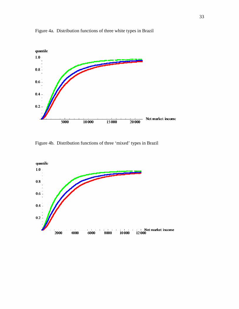
Figure 4a presents the distribution functions of disposable income for the

Brazilian types (white, male household head, urban), (white, female household head,

urban), (white, male household head, rural) in order of stochastic dominance (using the

Higgens-Pereira data set). Thus, it appears that one has better opportunities if one is

raised by a woman in the city than by a man in the countryside. Figure 4b presents the

analogous three distribution functions for the mixed race. The order of stochastic

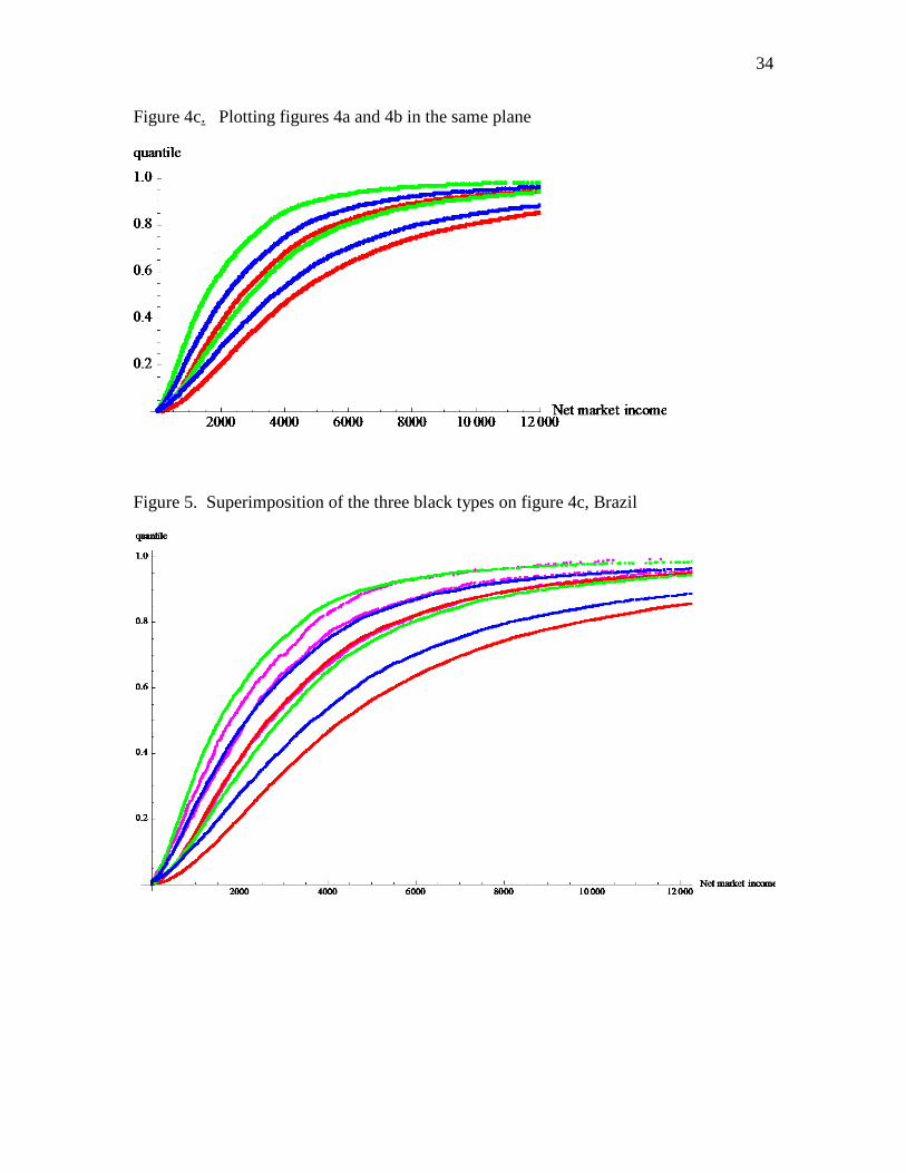
dominance is the same as in figure 4a. Figure 4c places these two plots together: we

see that even the most disadvantaged white type first-order-stochastic-dominates the most

advantaged mixed type.

It turns out that the three black types also have distribution functions ordered in

the same way. Figure 5 presents the distribution functions of the black types (in violet)

superimposed upon figure 4c. We observe that the first two black types ((male

household head, urban) and (female household head, urban)) have distribution functions

that are virtually coincident with the analogous mixed types, and the distribution function

of (black, male household head, rural) appears to FOSD the comparable ‘mixed’ type.

Indeed, the distribution function of the (black, male household head, urban) type is

virtually invisible in figure 5, as it coincides so closely with that of the (mixed, male

household head, urban) type. The conclusion appears to be that there is racial

discrimination in Brazil which favors whites over non-whites, but there is no special

19

discrimination against black workers, who appear, if anything, to have somewhat better

opportunities than ‘mixed’ workers.

Finally, Björklund, Jäntti and Roemer (2012) study income in Sweden, using a

large data set that permits the partition of the population into over 1100 types, based on

six circumstances, each partitioned into several levels. Using methods different from the

ones discussed here, they conclude that at least 25% of income inequality is due to

circumstances15. Contrast this to the 1.5% figure for Sweden from table 1.

5. Equity ‘versus’ development16

It is often said that equity and efficiency are competing goals -- that equity is

purchased at the expense of efficiency. There are two senses in which this phrase may

be uttered. The first is that redistributive taxation may be purchased only at the cost of

Pareto inefficiency, due to workers’ and firms’ facing different effective wages. The

second sense is that redistribution may lower total output. These two claims are in

principle independent. There may be policies which re-allocate income in a more

equitable manner, lower total output, but are not Pareto inefficient. (Think, for example,

of re-allocating educational funds from tertiary education to secondary education in a

poor country. This might have a purely redistributive effect, without significant

consequences for Pareto efficiency.)

I wish to criticize the second usage of the phrase. Saying that there may be a

trade-off between equity and efficiency where efficiency is measured as total output is

equivalent to saying there is a trade-off between equity and the utilitarian measure of

15 Perhaps, most critically, IQ in adolescence is taken as a circumstance. 16 The point in this section is discussed more extensively in Roemer (2006).

20

development, which (in its simplest form) is given by output per person. In fact, both the

measures of equity that I have proposed in the ordered pair d, and output per capita, are

measures of equity according to different normative criteria, as discussed in section 2.

Indeed, because utilitarianism was the reigning conception of distributive justice until at

least the 1970s, it is unsurprising that GDP per capita was the corollary measure of

development in economics.

There is an increasing number of economists who argue that ‘improving equity

improves efficiency.’ (The World Development Report (2006) presses this point, but the

argument goes back many years.) My objection is not to the substantive claim, that

equalizing opportunities often increases productivity and national income, but only to the

tradition of assigning utilitarianism primus inter pares as the normative view which

defines efficiency.

If the view of economic development I here advocate is adopted, there may be a

significant change in policy evaluation. One would not have to justify investment in very

disadvantaged social groups by showing that such investment increased total output. In

the long run, such a conflict might not exist: but often, policy makers must evaluate the

consequences of their policy choices in the short run. If a country is evaluated on the

basis of its ordered-pair statistic rather than on GDP per capita, policies could

be quite different.

6. A World-Bank proposal for measuring equal opportunity

The World Bank has been an important innovator in bringing considerations of

equal opportunity into economic development. Its two important publications, to date,

21

have been the 2006 World Development Report, Equity and Development, and a

monograph, Measuring inequality of opportunities in Latin America and the Caribbean

(Paes de Barros et al., 2009). The more recent publication contains a wealth of

information on the effects of social circumstances on various measures of achievement

and output.

Paes de Barros et al. (2009) propose a measure of equality of opportunity.

Consider a particular kind of opportunity, such as ‘attaining the sixth grade in elementary

school.’ Let the total sixth-grade attendance in a country be H, and the total number of

children of sixth-grade age be N, and define to be the access on average of

children to the opportunity of a sixth-grade education. measures the level of this

opportunity in the country, but not the extent to which access is unequal to different

children, based upon their social circumstances. Now using a logit model, estimate the

probability that each child, j, in the country has of attending the sixth grade, where that

probability is a function of a vector of circumstances; denote this estimated probability by

. Define . D measures the variation in access to the

opportunity in question across children in the country. The normalization guarantees that

. Now define the human opportunity index as

;

note that .

The human opportunity index is a non-consequentialist measure of development,

because the probabilities can only be computed knowing the circumstances of the

children. The measure combines a concern with the level of provision of opportunities

22

and the inequality of the distribution of them. This is to be contrasted with my ordered

pair , which separates these two concerns into two measures. Obviously, some

information is lost in using a single measure rather than two measures.

The concern of the 2009 report is in large part with children. In my view, where

children are concerned, all inequality should be counted as due to circumstances, and

none to effort, and so the fact that the human opportunity index does not explicitly make

the distinction between effort and circumstances is unobjectionable17. However, if the

measure is used for addressing inequality of opportunity for adults, this may be a defect.

To study this, let us take an opportunity for adults – earning an income above M,

measured in PPP exchange rates. Suppose there are three types of worker, according to

the level of education of their more educated parent. Denote the distribution of income in

type t as ; let the fraction of type t be and let F be the distribution of income in the

society as a whole. Then is the average access to the opportunity in

question in the country. Now for all members j of a given type, t, compute that

: this is because the probabilities are computed by taking the

independent variables in the logit regression as the circumstances. Hence, the human

opportunity measure is:

(12)

17 Children should only become responsible for their actions after an ‘age of consent’ is reached, which may vary across societies. Both nature and nurture fall within the ambit of circumstances for the child.

23

Despite the fact that effort is not explicitly mentioned in defining the index, effort is

reflected in measure, because the distributions appear in the calculation. Indeed, the

first term measures the level of opportunity in the country, while the second

term is a penalty for the degree to which this opportunity is mal-distributed with respect

to circumstances (e.g., if there were no inequality of opportunity, then

for all t, and the penalty is zero).

In expression (12), the first term on the right-hand side, , plays the role

that plays in my measure: it measures the level of development. But while

focuses upon how well off the most disadvantaged type is doing, is a level for

the society at large. The second component of my measure, η, is explicitly derived to

show the degree to which inequality is due to circumstances, while the second term on

the right-hand side of (12) is a form of a variance. Certainly these two measures are

getting at the same phenomenon. I have a slight preference for my proposal, as it is

more carefully justified as measuring what we are concerned with. But these are minor

criticisms; certainly, the measure O is in the spirit of thinking of economic development

as opportunity equalization.

7. Conclusion

Inequality has become an important focus in development economics in recent

years, and this is a step forward from the days when only GDP per capita was considered

to be salient. But an important weakness in the entry of inequality into the field has been

treating all inequality as having the same ethical status. This is seen in the very large

literature on the measurement of inequality, where the concern has been upon whether the

24

statistical properties of various inequality measures conform to our intuitions concerning

when equality is large or small. These discussions ignore the issue of whether inequality

is innocuous or undesirable – that is, the ethical status of the inequality. The equal-

opportunity literature introduced the latter distinction into economic theory, and it built

on the introduction of the issue of responsibility into egalitarian political philosophy,

through the writings of R. Dworkin (1981a,b), G.A. Cohen (1989) and R. Arneson

(1989). For discussions of this literature, from economists’ viewpoints, see Roemer

(1996, 2009) and the treatment of Fleurbaey (2008).

It is useful to further compare the equal-opportunity approach to inequality to the

approach represented by the human development index, based upon the work of Amartya

Sen on functionings and capability. As is well known, Sen’s (1980) major point was that

there are objective measures of human functioning that are important for any conception

of welfare, and the set of vectors of functionings, available to a person, which Sen

defined as her capability, is a measure of the opportunities that she has. Sen’s

intervention was post-Rawls and pre-Dworkin: his main foil was Rawls’s choice of

primary goods as the equalisandum, which he proposed replacing with capabilities; and

his conception of responsibility was implicit in the idea that, if capabilities, so defined,

were ‘equal’ (whatever that should mean) across persons, then if individuals chose

different vectors of functioning from these sets, the result was of no ethical consequence.

The treatment of responsibility, in Dworkin (1981,1982), was significantly more explicit,

and led to the equal-opportunity literature.

The proposal I have stated here, and the human development index (HDI), are

complementary. The HDI broadens the objective of concern from income (GDP) to a

25

set of functionings, but continues to average over the population as a whole, and ignores

the source of inequality18. The equal-opportunity approach – as I have advocated

applying it to a set countries – retains income as the objective, but disaggregates the

population into types based upon circumstances that are beyond the control of

individuals. The HDI approach says that human accomplishment along dimensions

other than income is important, and the equal-opportunity approach says that inequality is

bad only if it is of a certain kind.

Of course, it is possible to unite the two approaches. Instead of using income as

the measure in my proposal, one could measure human development disaggregated by

types, where type continues to be defined according to a set of circumstances, and then

the two-dimensional index d would allow us to assess levels and degrees of development

with regard to the various Sen-inspired functionings. It would be ideal to have data sets

that permitted us to do this. The reason I have here proposed using only income is that I

think, at this point, we do not have the data to compute the distribution of levels of

human development by type for a large set of countries. However, the recent publication

of the results of the Global Burden of Disease project ( see the entire issue of The Lancet,

December 13, 2012) indicates that this lacuna may be filled, as we may soon have

available distributions of longevity by country and by type19.

Note that the issue of the ethical status of inequality is quite different from

another way that inequality can be good or bad, and that is, with regard to its effect on

18 In the 2011 Human Development Report, the human development index is calculated by taking a geometric mean of national income, literacy, and longevity, rather than a convex combination of them. 19 In this issue of Lancet, longevity and morbidity figures are given for almost all countries in the world. Information on these measures of welfare by type is not, however, reported.

26

incentives. Bad inequality in this sense – inequality that is bad for incentives – will be

condemned by the utilitarian measure of GDP per capita, because its elimination will

increase social output. This is to be distinguished from inequality that is bad because it

reflects disadvantage due to circumstances: as I have emphasized, eliminating this kind of

inequality is not -- at least in the short run – synonymous with increasing total output or

welfare.

The equal-opportunity approach, which focuses upon eliminating inequalities that

are due to circumstances for which persons should not be held responsible, is both good

ethics and also good policy – by which I mean it is policy supported by the majority of

people in many countries. For we know from survey data that, globally, people believe

injustice occurs when low incomes are due to bad luck as opposed to low effort. What

differs across countries is the extent to which citizens attribute low incomes to bad luck

as opposed to low effort: in Brazil, a much larger fraction believe poverty is due to bad

luck than in the United States (and perhaps this reflects reality). Indeed, the popular

moniker associated with equality of opportunity – it levels the playing field -- can be

interpreted as a way of saying that disadvantages that some face due to circumstances

beyond their control should be eliminated before the competition for economic goods

begins.

27

References

Arneson, R. 1989. “Equality and equality of opportunity for welfare,”

Philosophical Studies 56, 77-93

Björklund, A., M. Jäntti, and J. Roemer, 2012. “Equality of opportunity and the

distribution of long-run income in Sweden,” Social choice and welfare 39, 675-696

Bourguignon, F., F. Ferreira and M. Walton, 2007. “Equity, efficiency and

inequality traps: A research agenda,” J. Econ. Inequality 5, 235-256

Checchi, D. and V. Peragine, 2010. “Inequality of opportunity in Italy,” J. Econ.

Inequality 8, 429-450

Checchi, D., V. Peragine, and L. Serlenga, 2010.“Fair and unfair inequalities in

Europe,” Working Paper No. 174, ECINEQ, Society for the study of economic

inequality, http://www.ecineq.org/milano/WP/ECINEQ2010-174.pdf

Cohen, G.A. , 1989. “On the currency of egalitarian justice, ” Ethics 99, 906-944

Dworkin, R. 1981a. “What is equality? Part 1: Equality of welfare,” Philosophy

& Public Affairs 10, 185-246

Dworkin, R. 1981b. “What is equality? Part 2: Equality of resources,” Philosophy

& Public Affairs 10, 283-345

Ferreira, F. and J. Gignoux, 2011. “The measurement of inequality of opportunity:

Theory and application to Latin America,” Rev. Income & Wealth 57, 622-657

Fleurbaey, M. 2008. Fairness, responsibility and welfare, Oxford University

Press

Fleurbaey, M. and V. Peragine, 2013. “Ex ante versus ex post equality of

opportunity,” Economica 80, 118-130

28

Gaertner, W. and E. Schokkaert, 2012. Empirical social choice, Cambridge

University Press

Higgens, S. and C. Pereira, in press. “The effects of Brazil’s high taxation and

social spending on the distribution of household income,” Public Finance Review

Paes de Barros, R., Ferreira, F., Molinas Vega, J. and Saavedra Chanduvi, J.

2009.Measuring inequality of opportunities in Latin America and the Caribbean,

Washington, D.C.: The World Bank

Rawls, J. 1971. Theory of justice, Harvard University Press

Roemer, J. 1993. “A pragmatic theory of responsibility for the egalitarian

planner,” Philosophy & Public Affairs 22, 146-166

Roemer, J. ,1996. Theories of distributive justice, Harvard University Press

Roemer, J. 1998. Equality of opportunity, Harvard University Press

Roemer, J. 2002. “Equality of opportunity: A progress report,” Social Choice &

Welfare 19, 455-472

Roemer, J. 2006. “Review essay: The 2006 World Development Report, ‘Equity

and Development’” , Journal of Economic Inequality 4, 233-244

Roemer, J. 2012. “On several approaches to equality of opportunity,” Econ. &

Phil. 28, 165-200

Sen, A. 1980. “Equality of what?” in S. McMurrin (ed.), The Tanner Lectures on

Human Values, Vol.1, Salt Lake City: University of Utah Press

Van de gaer, D. 1993. “Equality of opportunity and investment in human capital,”

Ph.D. dissertation, K.U. Leuven

29

World Bank, 2006. World Development Report: Equity and Development ,

Washington D.C.: The World Bank

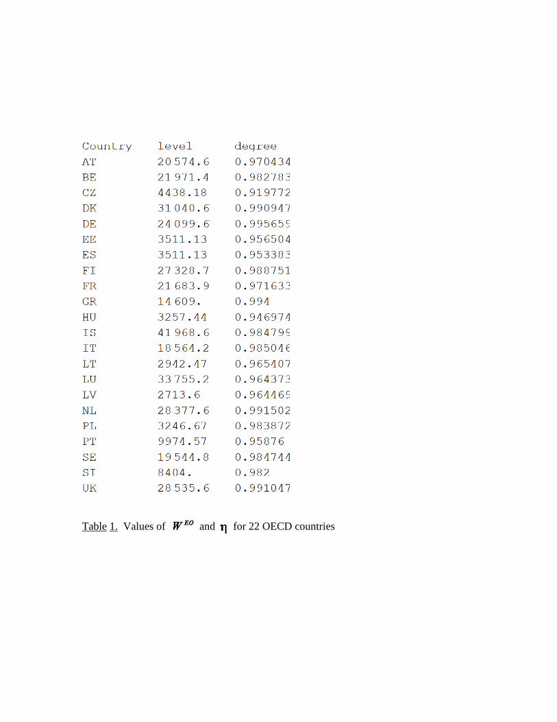
Table 1. Values of and for 22 OECD countries

31

Figures

Figure 1. CDFs of income for three types of Austrian male worker

Figure 2a. CDFs of income for three types of Hungarian worker

32

Figure 2b. CDFs of income for three types of Danish worker

Figure 3 Ordered pairs for European countries with best-fitting (least-quares)

regression line

33

Figure 4a. Distribution functions of three white types in Brazil

Figure 4b. Distribution functions of three ‘mixed’ types in Brazil

34

Figure 4c. Plotting figures 4a and 4b in the same plane

Figure 5. Superimposition of the three black types on figure 4c, Brazil

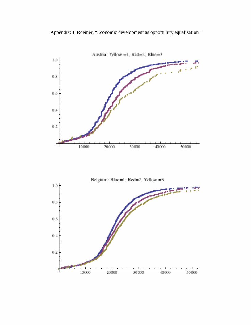
Appendix: J. Roemer, “Economic development as opportunity equalization”