Integr12.doc

Economic Integration, Imperfect Competition,

and International Policy Coordination*

by

Bertil Holmlund† and Ann-Sofie Kolm‡

First draft: January 1999

This version: 22 April 1999

AbstractThe paper examines policy externalities between imperfectly competitive open economies whereunemployment prevails in general equilibrium. We develop a two-country and two-sector modelwith monopolistic competition in the goods market and wage bargaining in the labor market.Policy externalities operate through the real exchange rate and economic integration is modeled asa reduction in trade costs. We explore how market integration influences policy spillovers,employment and real wages. We also examine how national and supranational commodity taxpolicies affect sectoral and total employment. Finally, we characterize optimal commodity taxeswith non-cooperative and cooperative policies and offer some rough estimates of the welfare gainsfrom policy coordination, using a calibrated version of the model.

JEL-Classification: D43, E61, F15, J23, J64.Keywords: Economic integration, imperfect competition, wage determination, policy cooperation.

* We gratefully acknowledge comments on an earlier draft of the paper from Peter Fredriksson, Claus Thustrup

Hansen and seminar participants at Norwegian School of Economics and Business Administration (Bergen),

Stockholm School of Economics, Stockholm University, Tilburg University and Uppsala University.† Department of Economics, Uppsala University, Box 513, SE-751 20 Uppsala, Sweden.

E-mail: Bertil Holmlund@nek.uu.se‡ Department of Economics, Uppsala University, Box 513, SE-751 20 Uppsala, and Office of Labour Market Policy

Evaluation (IFAU), Sweden. E-mail: Ann-Sofie.Kolm@nek.uu.se

1

1. Introduction

The European economic integration has brought issues regarding policy coordination to the fore in

recent policy debates and research efforts. The discussion has been concerned with economic

policies in general, including monetary and fiscal policies, as well as "structural" policies dealing

with taxes and regulations. The case for policy coordination relies on the idea that non-cooperative

outcomes fail to internalize various policy externalities. One channel for international policy

spillovers operates through the real exchange rate.

This paper contributes to the discussion about policy coordination regarding commodity

taxation. To that end we develop a two-country and two-sector general equilibrium model of

international trade where the real exchange rate is endogenously determined. The model features

imperfect competition in product and labor markets and unemployment prevails in general

equilibrium. The framework allows a positive analysis of the effects of market integration and the

nature of policy spillovers as well as a normative analysis of the gains from policy coordination.

The paper is related to and unifies two strands of recent contributions. One strand of literature

has primarily addressed positive issues and examined how product market integration affects wage

bargaining and employment in unionized economies.1 Papers by Andersen and Sørensen (1992),

Driffill and van der Ploeg (1993, 1995), Danthine and Hunt (1994), Huizinga (1993), Sørensen

(1994) and Naylor (1998) belong to this category. The modeling strategies differ across the papers,

and so do the results. Some of the studies model increased product market integration as a

reduction in trade costs; cf. Driffill and van der Ploeg (1993) and Naylor (1998). Other studies

assume that integration increases the elasticity of substitution between domestic and foreign

goods; see Andersen and Sørensen (1992) and Danthine and Hunt (1994). A third category,

represented by Huizinga (1994) and Sørensen (1994), compare two polar cases, autarky vs

perfectly integrated product markets. The fact that the different modeling approaches produce

different results comes as no surprise. In general, the effect of integration on bargained wages

depends on how integration affects the perceived wage elasticity of labor demand. Wage

moderation is the outcome if this elasticity increases, as in Andersen and Sørensen (1992) and

1 An earlier literature investigated the effects of integration on product markets by making use of the new tradetheories with monopolistic competition and increasing returns to scale; cf. Venables (1987), Smith and Venables(1986) and Venables and Smith (1988). These contributions did not address questions pertaining to imperfect labormarkets and wage bargaining.

2

Danthine and Hunt (1994). Increased wage pressure is the result if the labor demand elasticity is

reduced, as in the model of oligopolistic rivalry in Naylor (1998).

The other strand of related literature has explored the case for policy coordination among

economies with integrated product markets. Andersen and Sørensen (1995) as well as Andersen,

Rasmusen and Sørensen (1996) analyze optimal fiscal policies with and without international

cooperation. The main result is that uncoordinated fiscal policy is too expansionary. Similar results

were obtained – in models without labor market distortions – in earlier contributions by van der

Ploeg (1987), Turnovsky (1988) and Devereux (1991). The reason for the overexpansion result is

that a government that acts non-cooperatively has an incentive to use fiscal policy as a means to

improve the country's terms of trade.

Our study differs from and extends the previous contributions in several respects. We include a

non-tradable sector in the analysis, which makes it possible to examine sector-specific policies. In

particular, the two-sector framework allows an analysis of how employment and welfare at home

and abroad is affected by, for example, sectorally differentiated value added taxes (or payroll

taxes). This is of obvious relevance for the ongoing discussions within the European Union

regarding harmonization of value added taxes; one issue in this discussion is whether there should

be supranational rules concerning the member countries' policies regarding sectoral tax

differentiation. In general, a case can be made for some sectoral differentiation of value added

taxes, but whether there is any rationale for policy coordination in this area is an open question.

Our analysis sheds light on this issue.

The two-sector framework is important in the analysis also for another reason. Our model of

equilibrium unemployment features complete real wage flexibility with respect to general changes

in labor or commodity taxes, a wellknown feature of many models of equilibrium unemployment.2

The main reason for this property of the model is that we assume that the real unemployment

compensation is indexed to the real after-tax consumer wage through a fixed replacement ratio.

Absent a non-tradable sector, this assumption implies that unemployment in an open economy

would be invariant to changes in the real exchange rate. Unemployment would then be determined

by an aggregate wage setting schedule that could be drawn as a vertical line in the real wage and

(un)employment space and domestic employment policies would have no effect on foreign

employment. However, the presence of a non-tradable sector implies that policies concerning

2 See, for example, Johnson and Layard (1986), Layard et al (1991) and Pissarides (1991, 1998).

3

domestic employment may have repercussions on foreign employment through sectoral

reallocation effects, as induced changes in the real exchange rate affect the sectoral allocation of

labor. These reallocation effects may in turn affect total employment, a possibility that follows

from our model of an imperfect labor market where sectoral wages are not necessarily equalized.

Economic integration would seem to make issues concerning international policy linkages

more relevant than they otherwise would have been. One might conjecture that policy externalities

among countries would increase in importance as barriers to trade are removed; of course, no

international policy spillovers would exist under complete autarky. However, our analysis shows

that there is no simple association between the removal of trade barriers and the magnitude of

policy spillovers. Although domestic policies in general affect foreign employment through

adjustments of the real exchange rate, we show that these spillover effects vanish as trade costs

approach zero and product markets thus become completely integrated.

We proceed by presenting the model in the next section of the paper. In section 3 we take a

look at some implications of increased market integration. Section 4 is devoted to a positive

analysis of international repercussions of tax policies; we focus on how national and supranational

policies concerning commodity taxes affect sectoral and total employment in the two countries.

Section 5 includes an analysis of optimal commodity taxation and Section 6 concludes.

2. The Model

2.1 Brief Outline

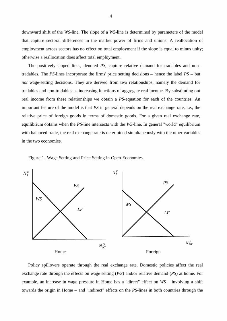
We begin with a brief overview of the main ingredients of the model by means of Figure 1. There

are two countries, Home (H) and Foreign (F). In each country there are two sectors, a tradable (T)

and a non-tradable (NT) sector. Tradables and non-tradables are produced in many varieties. Total

employment in the tradable sector is denoted NTj whereas total employment in the non-tradable

sector is denoted N NTj , j=H, F. Labor is the only factor of production. In Figure 1, the dashed and

negatively sloped 45-degree lines denoted LF represent the labor force constraints in the countries.

In an economy with full employment, the feasible employment combinations would coincide with

the labor force constraint. With imperfect labor markets, the feasible employment combinations

are located to the left of the labor force constraint, as illustrated in Figure 1 by the WS-lines. These

lines are derived from wage setting behavior; hence the label WS. The position of a WS-line is

determined by labor and product market characteristics within a country. An increase in wage

pressure, caused by, say, higher unemployment benefits or more powerful unions, produces a

4

downward shift of the WS-line. The slope of a WS-line is determined by parameters of the model

that capture sectoral differences in the market power of firms and unions. A reallocation of

employment across sectors has no effect on total employment if the slope is equal to minus unity;

otherwise a reallocation does affect total employment.

The positively sloped lines, denoted PS, capture relative demand for tradables and non-

tradables. The PS-lines incorporate the firms' price setting decisions – hence the label PS – but

not wage-setting decisions. They are derived from two relationships, namely the demand for

tradables and non-tradables as increasing functions of aggregate real income. By substituting out

real income from these relationships we obtain a PS-equation for each of the countries. An

important feature of the model is that PS in general depends on the real exchange rate, i.e., the

relative price of foreign goods in terms of domestic goods. For a given real exchange rate,

equilibrium obtains when the PS-line intersects with the WS-line. In general "world" equilibrium

with balanced trade, the real exchange rate is determined simultaneously with the other variables

in the two economies.

Figure 1. W age Setting and Price Setting in O pen Econom ie s .

H om e Fore ign

Policy spillovers operate through the real exchange rate. Domestic policies affect the real

exchange rate through the effects on wage setting (WS) and/or relative demand (PS) at home. For

example, an increase in wage pressure in Home has a "direct" effect on WS – involving a shift

towards the origin in Home – and "indirect" effects on the PS-lines in both countries through the

NNTD

PS

WS

PS

WS

NTF

LFLF

N NTF

NTH

5

real exchange rate. A reduction in the tax on domestic tradables has a direct effect on PS in Home,

raising the demand for tradables and inducing a reallocation of employment towards the tradable

sector. The increased supply of tradables in Home relative to the supply of tradables in Foreign

causes an adjustment of the real exchange rate, i.e., an increase in the price of foreign tradables

relative to the price of domestic tradables. This relative price adjustment affects the sectoral

allocation of employment in Foreign, and possibly total employment as well.

This completes the brief overview of the model. We proceed to the details.

2.2 Consumers

We normalize the number of individuals in each country to unity. There is no labor mobility

between countries. The following characterization pertains to Home; analogous descriptions hold

for Foreign. Individual i consumes traded ( )CiTH and non-traded ( )CiNT

H goods and has a utility

function given as:

(1) ΛiiTH

iNTHC C=

−

−

α α

α α

1

1

, 0 1< <α .

Labor is supplied inelastically without loss of utility. Both tradables and non-tradables appear in

many varieties and the sub-utility functions for the different varieties are given as:

(2)C C

C C

iTH

ijj

K

iNTH

iK

T

NTH

=

=

−

=

−

−

=

−

∑

∑

µµ

µµ

σσ

σσ

1

1

1

1

1

1

,

,ll

µ σ, > 1.

There are KT varieties of tradables; KTH of these are produced in Home and K KT T

H− in Foreign.

The number of varieties of non-tradables in Home is given by KNTH . The number of varieties

produced in each of the countries is exogenous. The parameter µ ( )σ is the elasticity of

substitution between any two tradable (non-tradable) goods.

The individual receives unemployment benefits, B, if he is unemployed and labor income, Wi ,

if he is employed in one of the sectors. Profits are distributed equally to all individuals as

6

dividends, π . The individual's income is thus given as I Wi i= + π if he is employed and as

I Bi = + π if he is unemployed. The budget constraint takes the form:

(3) I P C P C P Ci hH

h

KihH

fH

f K

KifH HK

iHT

H

TH

T NTH

= + += = =∑ ∑ ∑~ ~ ~

1 1 ll l .

The consumer (producer) price of tradables produced in Home is denoted ~PhH ( Ph

H ), whereas ~PfH

( PfH ) is the domestic consumer (producer) price of tradables produced in Foreign. ~P H

l ( PHl ) is

the consumer (producer) price of non-tradables in Home. C CihH

ifH, , and Ci

Hl are the domestic

consumer's demand for domestically produced tradables, foreign produced tradables, and non-

tradables. Destination-based value added taxes, denoted tTj and tNT

j for j=H, F, create a wedge

between consumer and producer prices, i.e., ~ ( )P P thH

hH

TH= +1 , ~ ( )P P tf

HfH

TH= +1 , and

~ ( )P P tH HNTH

l l= +1 for consumer prices in Home. Our results are independent of whether value

added taxes are destination-based or origin-based.3 Moreover, value added taxes and payroll taxes

are equivalent in our model so all results can be obtained by sectoral differentiation of payroll

taxes.

The individual demand for the specific goods is derived by maximizing the utility function

given by (1) and (2), subject to the budget constraint in (3). From this maximization we derive the

aggregate domestic demand function pertaining to a specific firm. This takes the form

(4) CPP

IPh

H hH

TH

H

TH=

−

αµ~

~ ~ , h=1,..., KTH ,

for a firm that produces tradables in Home. I H is the aggregate domestic income whereas ~PTH is

the general price index for tradables relevant for domestic consumers:

(5) ( )~ ~P PTH

jH

j

KT=

−

=−∑ 1

1

11µ µ = ( ) ( )( )K P K K PT

HhH

T TH

fH~ ~1 1

11− − −+ −

µ µ µ .

Some of the prices in the price index are set by foreign firms. The expression in the rightmost

bracket is derived by assuming symmetric conditions for firms within each country.

3 This is in contrast to the analysis in Lockwood (1993) of commodity tax competition under perfect competition,

where a switch from the destination principle to the origin principle does affect the equilibrium outcome.

7

A firm in Home producing tradables faces also foreign demand for its product. With equal

preferences in the two countries, the aggregate demand relevant for such firm is given by:

(6) C C CPP

IP

PP

IPh h

HhF h

H

TH

H

TH

hF

TF

F

TF= + =

+

− −

αµ µ~

~ ~~~ ~ , h=1,..., KT

H .

~PhF is the price of tradable h produced in Home facing consumers in Foreign, and ~PT

F is the

general price index for tradables relevant for foreign consumers. I F is the aggregate income level

in Foreign. Analogous derivations yield the demand relevant for a firm that produces non-

tradables.4 The general consumer price index in Home, denoted ~P H , is obtained as a weighted

geometric average of the price of tradables, ~PTH , and the price of non-tradables, ~PNT

H , i.e.,

( ) ( )~ ~ ~P P PHTH

NTH=

−α α1. The general consumer price index in Foreign is given in an analogous

way.

2.3 Firms

In each country there are a large number of firms that produce tradables and non-tradables. A

particular variety is produced by only one firm. Labor is the only factor of production, the

production technology is linear and all productivity parameters are normalized to unity. Exports

involve ("iceberg") transport costs proportional to the export value. Markets are segmented

because of transport costs and prices for identical products can differ across countries. Firms set

prices to maximize profits, taking wages as given. The objective function for a representative

domestic firm in the tradable sector can be written as:

(7)( ) ( )Π h h

HhH

hF

hF

h hF

hH H

hF

hF

hH

hH

hF

hF H

h hF

hHP C P C W C C F P C P C P C W C C= + − + − = + − +/ .τ

Wh is the nominal wage and F H the transport cost, where F H ∈ [ , )0 1 and τH HF≡ −1 1/ ( ) .

F H = 0 implies τH = 1 . The product markets are completely integrated when τ j = 1, j=H, F.

The following price setting rules are obtained for domestic and foreign markets:

4 The demand function is for a specific firm in the non-tradable sector is: CP

PIP

HH

NTH

H

NTHl

l= −

−

( )~

~ ~1 ασ

, l=1,..., KNTH .

8

(8) P WhH

T h= κ ,

(9) P P WhF H

hH H

T h= =τ τ κ .

κ µ µT ≡ −/ ( )1 is the usual markup factor. The optimal price in the foreign market is, in general,

higher than the domestic price due to transport costs. Once prices are set we obtain output and

employment from the relevant demand functions. By aggregating over the domestic firms and

using the relationships between consumer and producer prices we obtain the following aggregate

labor demand schedule for the domestic tradable sector:

(10) ( )NK I

P tPP

I tI t

PPT

H TH H

hH

TH

hH

TH

FTH

HTF

hH

TF

H=+

+ +

+

− −−α τ

µ µµ

( )( )( )111

1 1

,

where P P tTH

TH

TH= +~ / ( )1 and P P tT

FTF

TF= +~ / ( )1 are producer price indexes. Aggregate

demand for labor in the tradable sector depends on the relative price of domestic goods in the

home market, P PhH

TH/ , as well as the relative price of domestic goods in the foreign market,

P PhH

TF/ . It also depends on the aggregate real income in Home and Foreign.

It will be convenient to define the real exchange rate as p P PfF

hH≡ / . By using the

expressions for the price indexes for tradables in Home and Foreign we can rewrite (10) and

obtain

(10′) ( ) ( ) ( )NI

P tk p

I tI t

k pTH

H

hH

TH T

FF

TH

HTF

HT

H=+

+

+ +

++

− − −

− − − −− −α τ τ τ

µ µ µ µ µ

( )( )( )1

111

1 1 11 1 1 1

1

,

where k K K KT TH

T TH≡ −/ ( ) . A rise in p, i.e., a real depreciation, increases labor demand in the

domestic tradable sector. In general equilibrium we also need to consider adjustments in real

incomes, something that we do in the subsequent analysis.

Analogous reasoning can be used to derive pricing rules for firms in the non-tradable sector;

we get P WHNTl l= κ , where κ σ σNT ≡ −/ ( )1 . In a symmetric equilibrium, the demand for labor

in the non-tradable sector is given by ( )N I PNTH H H= −1 α / ~

l .

2.4 Wage Determination and the Labor Market

9

There is one union in each firm and each union cares about the utility of its members. The indirect

utility function for the worker is given as Λi iHI P∗ = / ~ , where Ii is the state-dependent income.

The time horizon is infinite and workers are concerned with their expected lifetime utility,

recognizing the possibility of transitions across sectors and labour force states. (See Appendix A

for details on the labor market structure.) Let Vh denote the expected lifetime utility of a worker

employed in a particular firm h in the tradable sector, Vl the expected lifetime utility of a worker

employed in a firm l in the non-tradable sector, and Vu the expected lifetime utility of an

unemployed worker. The nominal wage is set in decentralized union-firm negotiations, taking the

general price and wage levels as given. Wages are chosen according to Nash bargains where the

objectives are of the form:

( )[ ] [ ]m a x n W V W V W PW

h h h h h u h hH

h

TH

TH

Ω Π= −−

( ) ( ) ( ) / ~λ λ1,

( )[ ] [ ]m a x n W V W V W PW u

HNTH

NTH

ll l l l l l lΩ Π= −

−( ) ( ) ( ) / ~λ λ1

.

The union's contribution to the Nash bargain is given by its "rent", i.e., n V Vh h u( )− for the

tradable sector, and n V Vul l( )− for the non-tradable sector, with employment at the firm level

denoted nh and nl . The parameters λTH and λNT

H measure the relative bargaining power of the

unions relative to the firms, with λiH ∈ ( , ]01 , for i=T, NT. The wage bargains recognize that the

firms unilaterally determine employment once wages are set. The real wages in Home implied by

the bargains are:

(11)WP

VhH

TH

H~ = + −

−

λ µµ

11

, h=1,..., KTH ,

(12)WP

VHNTH

Hl~ = + −−

λ σσ

11

, l=1,..., KNTH .

The wage is set as a constant markup on V H , which is the per period value of unemployment

adjusted for dividends.5 The markups capture the market power of the unions relative to the firms

and are increasing in λTH and λNT

H and decreasing in σ and µ . Note that a rise in σ or µ

increases the elasticity of labor demand and profits with respect to wage changes. By symmetry,

5 V rV PHu

H≡ − π / ~ , where r is the discount rate (see Appendix A for details).

10

wages are set equal across bargaining units within each sector in equilibrium, i.e., W Wh TH= and

W WNTH

l = . From eqs. (11) and (12) we obtain the relative wage as Z W WHNTH

TH≡ / . Since all

workers face the same opportunities the relative wage takes the form:

(13)( )( )( )( )Z H NT

H

TH

=− + −− + −

µ λ σσ λ µ

1 1

1 1.

The relative wage is thus fixed by preference parameters and the measure of union bargaining

power. The value of unemployment net of dividends is, under our assumption of no discounting,

obtained as a weighted average of the utilities in the different states; the weights are given by the

employment rates, NTH and N NT

H , and the unemployment rate, U H :

(14) V NWP

NWP

UBP

HTH T

H

H NTH NT

H

HH

H

H= + +~ ~ ~ .

The wage equations in (11) and (12) can be expressed as an equilibrium relationship between

employment in the two sectors by eliminating V H by means of (14) and by using the labour force

identity, i.e., 1 = + +N N UTH

NTH H . The resulting employment relationship takes the form:

(15) NZ b

bNT

H HH H

H NTH= − −

−

ψ

1,

where ψ H <1 is a constant.6 The parameter bH is the fixed replacement rate with unemployment

benefits indexed to the average wage in the tradable sector, i.e., B b WH HTH= ; no results would

change if benefits instead were indexed to the wage in the non-tradable sector. The inequalities

b ZH H< and bH < 1 must hold as participation constraints. As (15) reveals, there is a tradeoff

between employment in the two sectors; indeed, this is the WS-line for Home as illustrated in

Figure 1. The relative wage, Z H , plays a crucial role for this tradeoff. An increase in employment

in the non-tradable sector is exactly offset by a decrease in employment in the tradable sector if the

relative wage is unity, i.e., Z H = 1. However, an expansion of non-tradable employment is not

completely offset by a decline in employment in the tradable sector if Z H < 1, and it is more than

6 [ ]ψ λ λ µHTH

TH Hb≡ − + − − −1 1 1 1( ) ( ) .

11

offset if Z H > 1. A rise in the market power of unions or firms, or a higher replacement rate,

produces a shift to the left of the WS-line by reducing ψ H .

To understand the employment tradeoff, consider an exogenous increase in the demand for

labor in the non-tradable sector and assume Z H < 1. This raises wage pressure and thereby crowds

out employment in the tradable sector. A wage premium for workers in the tradable sector,

Z H < 1, moderates the increase in wage pressure since the relative probability of finding a job in

the high-wage sector has decreased. The rise in employment in the non-tradable sector is in this

case not completely offset by lower employment in the tradable sector.

2.5 General Equilibrium

General equilibrium with a balanced government budget implies balanced trade. We can write the

trade balance expression as:

(16) ( )TB K P C K K P CTH H

hH

hF

T TH F

fF

fH= − −τ τ ,

where the first term represents the value of exports and the second term the value of imports.

Recall that τHhH

hFP P= is the price foreigners pay for tradables produced in Home (net of value

added taxes in Foreign); analogously, τFfF

fHP P= is the price domestic consumers pay for

tradables produced in Foreign (net of domestic value added taxes). From the individuals' utility

maximization we obtain the aggregate domestic demand for tradables produced in Foreign as well

as foreigners' aggregate demand for tradables produced in Home. By making use of the price

indexes for tradables relevant for domestic and foreign consumers, we obtain the trade balance

condition (TB=0) as:

(17)( )( )

II

tt

k p

k p

tt

f pF

HTF

TH

TH

TF

TF

TH

H F= ++

+

+≡ +

+

− − −

− −

11

1

1

11

1 1 1

1 1

τ

ττ τ

µ µ

µ µ( ; , ) .

Straightforward calculations yield the following partial derivatives: f p (.) < 0 , f Hτ (.) > 0 and

f Fτ (.) < 0 . A rise in p – a real depreciation – improves the trade balance, which has to be offset

by a decline in foreign income relative to domestic income so as to maintain external balance. A

rise in transport costs in Home, τH , worsens the trade balance, which requires an offsetting rise in

foreign relative income. Analogous arguments hold for changes in transport costs in Foreign.

12

We have now derived the relationships needed to characterize the general equilibrium. It will

be convenient to make use of the equations for the WS- and PS-lines. To that end we first represent

the equilibrium in each country by the following equations:

(18) NZ b

bNT

j jj j

j NTj= − −

−

ψ

1 j=H, F

(19) ( ) ( )NI

W tpT

jj

T Tj

Tj

j h F=+

ακ

τ τ1

Γ ; , j=H, F

(20)( )

( )NI

W tNTj

j

NT NTj

NTj

= −+

11

ακ

j=H, F

(21)( )( )( )( )Z D NT

j

Tj

=− + −− + −

µ λ σσ λ µ

1 1

1 1j=H, F

where

(22)( ) ( )

( )ΓH TF H

TF

k p

k p(.) ≡

+

+

− − −

− −

τ τ

τ

µ µ

µ µ

1 1 1

1 1,

and

(23)( ) ( )

( )ΓF TH F

TH

k p

k p(.) ≡

+

+

− − − −

− − −

1 1 1 1

1 1 1

τ τ

τ

µ µ

µ µ.

Eq. (18) reproduces (15) and represents the tradeoff between employment in the two sectors,

i.e., the WS-line. Eqs. (19) and (20) represent the aggregate demand for labor in the two sectors for

each country. To derive (19) for Home we use eq. (10) and the trade balance condition (17); the

derivation is analogous for Foreign. The aggregate demand relationships for the tradable sectors

thus incorporate the trade balance condition through ΓH (.) and ΓF (.) with the following partial

derivatives: ΓpH (. ) ,≥ 0 Γ

τ HH (.) ,< 0 Γ

τ FH (.) > 0 ,Γp

F (. ) ,≤ 0 Γτ HF (.) ,> 0 and Γ

τ FD (.) .< 0

Eqs. (18) - (21) for Home (Foreign) yield domestic (foreign) sectoral employment and real

domestic income, conditional on p. To derive the equations for relative labor demand we use (19)

and (20) to obtain:

(24) ( )N N A Z pTj

NTj j j j H F= θ τ τΓ ; , , j=H, F.

13

A NT T≡ −ακ α κ/ ( )1 is a constant and ( ) ( )θjNTj

Tjt t≡ + +1 1/ captures relative tax pressure, i.e.,

the tax pressure in the non-tradable sector relative to the tradable sector. Eq. (24) is the positively

sloped PS-schedule, as illustrated in Figure 1 above. The employment levels in the two domestic

and the two foreign sectors, conditional on p, are thus obtained from eqs. (18) and (24). We note

that taxes only affect sectoral and total employment through the relative tax pressure. The fact that

total tax pressure does not matter for employment outcomes is essentially driven by two features

of the model, namely the iso-elastic utility functions and the fixed replacement rates.7

It remains to determine the real exchange rate, i.e., the relative price between foreign and

domestic tradables. This is obtained by making use of two relationships: (i) the demand for

foreign tradables relative to the demand for domestic tradables, and (ii) the supply of foreign

tradables relative to the supply of domestic tradables. To obtain the relative demand schedule we

use the two equations in (19) together with the trade balance condition (17), recognizing that

prices are set as markups on wages. The resulting relationship gives the demand for foreign

tradables relative to domestic tradables as a function of the real exchange rate and trade costs,

i.e.,

(25)NN

pp

f p pTF

TH

F H F

H H FH F= −Γ

Γ( ; , )( ; , )

( ; , )τ ττ τ

τ τ 1 ,

where the right-hand side is decreasing in p. A rise in p, i.e., a fall in domestic relative prices,

increases the demand for domestic tradables relative to foreign tradables.

To obtain the relative supply schedule we use eqs. (18) and (24) to solve for NTH and NT

F as

functions of p. The outcome is the following relationship

(26)NN

Z b A Z p bZ b A Z p b

TF

TH

F

H

H H H H H H

F F F F F F= ⋅ + − −+ − −

− −

− −ψψ

θθ

1 11 1

1 1

1 1( )[ ( )] ( )( )[ ( )] ( )

ΓΓ

,

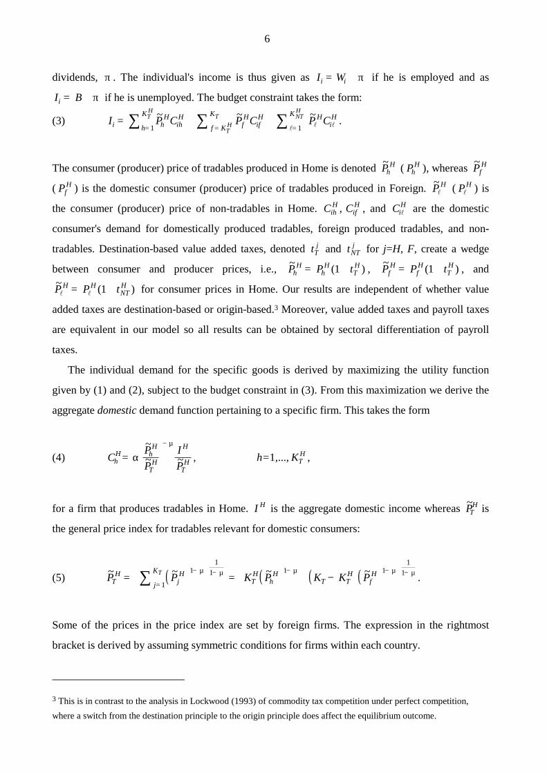
where the right-hand side is non-increasing in p. Eqs. (25) and (26) are illustrated in Figure 2. It is

easily verified that the slope of (25) is steeper than the slope of (26), the reason being that (26)

7 Many models of equilibrium unemployment have the property that labor and commodity taxes are completely borne

by labor if unemployment benefits are indexed to after-tax real wages; see, for example, Pissarides (1998).

14

incorporates wage adjustments to changes in the real exchange rate whereas eq. (25) is a demand-

side relationship that holds conditional on wages.8

Figure 2. Th e Determ ination of th e R eal Exch ange Rate.

We use eqs. (25) and (26) to equate relative demand and relative supply and obtain:

(27) Q f p pH F≡ −−( ; , )τ τ 1 ψψ

τ τ θτ τ θ

F

H

H H F H H H H H

F H F F F F F Fp Z b A Z bp Z b A Z b

⋅ + − −+ − −

=− −

− −ΓΓ

( ; , ) ( )[ ] ( )( ; , ) ( )[ ] ( )

1 1

1 111

0 ,

Eq. (27) implicitly determines p; note that Qp < 0 holds. Eq. (27) together with eqs. (18) and (24)

determine sectoral employment in each of the two countries along with the real exchange rate.

This completes the description of the model. We now turn to an investigation of the effects of

market integration and the nature of policy spillovers.

3. The Effects of Market Integration

3.1 Market Integration and Spillover Effects on Employment

We note from eqs. (18), (24) and (27) that international policy spillovers on employment work

through ΓH (.) and ΓF (.) , which involve the trade balance condition. Changes in the real

exchange rate will in general affect employment in both countries, so policies in one country that

affect p will thereby also influence employment in the other country.

How does increased market integration, i.e., a reduction in trade costs, affect these spillover

effects? From (22) and (23) we can conclude that there will be no spillover effects on employment

if (i) transport costs are infinitely high or if (ii) transport costs are zero. More specifically we have:

8 The relative supply schedule is horizontal if product markets are completely integrated, i.e., if τ j = 1 , j=H, F.

NN

TF

TH

p

( )25

( )26

15

Proposition 1. (i) Infinitely high transport costs: τH → ∞ implies ΓH → 1; analogously, τF → ∞

implies ΓF → 1. (ii) Zero transport costs: τH = 1 implies ΓH = 1; analogously, τF = 1 implies

ΓF = 1.

The fact that spillover effects on employment are absent when transport costs are infinitely

high is obvious since there will be no trade in this case. To understand the second and less

obvious part of the proposition, note that balanced trade implies that any decline in imports has

to be matched by a corresponding decline in exports. An increase in p causes an increase in the

domestic consumers' demand for domestic tradables and a reduction in the imports of tradables.

External balance requires an offsetting fall in the foreign demand for domestic goods through a

decline in foreign income relative to domestic income, as revealed by eq. (17). The resulting

substitution of domestic demand for foreign demand has no effect on domestic labor demand

when τH = 1, since this implies that the prices of domestic tradables are the same at home and

abroad. The purchasing power of foreign income in terms of domestically produced goods is thus

the same as the purchasing power of domestic income and the reallocation of spending patterns

have no real effects. With positive transport costs, however, a reallocation of spending induced

by a rise in p does matter for domestic labor demand. The purchasing power of foreign income in

terms of domestic tradables is lower than that of domestic income, which implies that the

demand for domestic labor increases when domestic demand is substituted for foreign demand.9

The result that spillover effects on employment vanish as markets become completely

integrated does not imply absence of policy externalities with respect to social welfare. Changes

in the real exchange rate affect welfare directly, through relative prices, even if there is no effect

on employment. This implies, as discussed in section 5, that policy externalities prevail even if

markets are completely integrated.

From here on we will, unless stated otherwise, present results that hold for strictly positive

transport costs. Results for the case with zero transport costs are easily obtained as special cases

with Γ ΓH F= = 1.

9 Holmlund and Kolm (1997) examine the effects of environmental tax reforms in a model of a small open economy

with the same labor market structure as the one adopted here. Since they assume zero trade costs, there will be no

employment effects arising from changes in the real exchange rate.

16

3.2 Market Integration, Employment and Real Wages

We have noted that several recent papers have analyzed how economic integration would affect

wage bargaining and ultimately employment. Closer integration, i.e., a reduction in trade costs,

have both direct and indirect effects as domestic employment is a function of ΓH H Fp( ; , )τ τ ,

whereas foreign employment is a function of ΓF H Fp( ; , )τ τ . We first consider the effect of

domestic transport costs, τH , on the real exchange rate.

A rise in τH implies that foreign consumers have to pay higher prices for tradables produced

in Home relative to tradables produced in Foreign. This shifts demand towards tradables

produced in Foreign. A rise in τH also worsens the trade balance, which requires an offsetting

rise in foreign income relative to domestic income; cf. eq. (17). This effect reinforces the rise in

the relative demand for foreign tradables and p tends to increase.

Eq. (26) incorporates wage adjustments to higher domestic transport costs and the sectoral

reallocation of workers. There will be a reallocation of workers from the tradable towards the non-

tradable sector in Home, whereas the opposite movements take place in Foreign. This implies that

the supply of tradables produced in Home falls relative to tradables produced in Foreign. Referring

to Figure 2, there will be an upward shift of the relative supply schedule, which tends to reduce p.

However, this negative supply effect on p never dominates the positive demand effect. From

inspection of (27) we can conclude:

Proposition 2. An increase in domestic trade costs ( )τH increases p.

The effects of trade costs on employment are, however, ambiguous. We can decompose the

total effect on domestic employment as follows

(28)dNd

Np

piH

jiH

H

H

j

H

jτ∂∂Γ

∂Γ∂τ

∂Γ∂

∂∂τ

= +

,i T NTj H F==

,,

where ∂ ∂ΓNTH H/ > 0 and ∂ ∂ΓN NT

H H/ < 0 . The first term in the bracket captures the direct (p-

constant) effect, whereas the second term reflects the indirect effect operating through the real

exchange rate. To sign (28) we need to sign the bracketed expression.

17

Consider the effect on NTH of a rise in domestic transport costs. The first term within brackets

in (28) is negative, reflecting the fall in foreign demand for domestically produced tradables. This

effect is counteracted by an induced increase in p, which raises the demand for domestic tradables.

The net effect on NTH is ambiguous, which implies that the effect on N NT

H is ambiguous as well.

Hence, the effect on total employment is also ambiguous.

A global reduction in transport costs ( τ τ τH F= = ) has no effect on the real exchange rate if

there is complete symmetry between the countries.10 The second term in the brackets of (28) then

drops out. A symmetric reduction in τ has, however, an ambiguous effect on ΓH (.) , so it is in

general impossible to sign the employment effects even in a wholly symmetric world.

We next ask how a global reduction in trade costs affects real consumer wages. There is no

wage response in partial equilibrium, as is revealed by eqs. (11) and (12); this is an implication of

the fact that technologies and union objective functions are iso-elastic. In general equilibrium,

however, there will be real wage adjustments to economic integration. These arise for a number of

reasons. The direct effect involves a fall in consumer prices due to lower import prices, and hence

a rise in real wages. In addition there may be indirect effects working through the real exchange

rate and the tax rate (via the government's budget restriction).11 The net effect cannot be

determined in general, but there is a presumption that real wages will rise as trade costs fall. This

is certainly the case when countries as well as sectors are symmetric.12 The real wage is then given

as

(29) [ ]WP

K tj

jj

~ ( )/ ( )

= + +∗ − − − −κ τ µ α µ1 1 1 1

1 1 , j=H, F

where K∗ is a constant.13 The tax rate is fixed by the government budget restriction once total

employment is determined. The effect on the real wage of a symmetric increase in trade costs is

obtained as:

10 By symmetric countries (a symmetric world) we mean that the parameters of the economies do not differ across

the two countries. However, the number of firms in the non-tradable sectors are irrelevant for the aggregate outcomes

and need not be restricted.11 The government's budget restriction is given as: t P C t P C P C N N bWNT

H HNTH

TH

hH

hH

fH

fH

NT T Tl + + = − −( ) ( )1 . A

balanced budget can always be achieved through adjustment of tTH or tNT

H while keeping θH fixed.12 By symmetric sectors we mean µ σ= and λ λT

jNTj= , and thus Z j =1 for j=H, F.

13 ( ) ( )K K KT NT∗ − − −≡ α µ α σ/ ( ) ( ) / ( )1 1 1 .

18

d W Pd

j jln( / ~ )τ

αττ

µ

µ= −+

<−

−101 , j=H, F.

The real exchange rate remains fixed at unity and the tax rate does not change since total

employment is not affected if the sectors are symmetric. The equilibrium real wage thus

increases when trade costs fall.

In conclusion, we have seen that there can be no presumption that market integration would

strengthen policy spillover effects concerning employment; in fact, those spillover effects vanish

as markets become completely integrated. The effects of market integration on sectoral and total

employment are in general ambiguous whereas the effect on real wages is likely to be positive.

3. The Effects of National and Supranational Tax Policies

We now turn to the employment effects of commodity taxation. The national policy is represented

by the relative tax pressure in Home, i.e., ( ) ( )θHNTH

THt t≡ + +1 1/ ; recall that the total tax pressure

has no effects on sectoral or total employment. The analysis of foreign policies is analogous and

therefore omitted. We also examine the consequences of supranational (global) policies, i.e.,

simultaneous changes of domestic and foreign policies. The government's budget is always

balanced.

Consider first a domestic policy that increases the relative tax pressure in Home, i.e., a policy

that raises the tax on non-tradables relative to the tax on tradables. By making use of eqs. (18),

(24) and (27), we can conclude:

Proposition 3. An increase in domestic relative tax pressure ( θH ) increases p and N NTH

NTH/ , but

reduces N NTF

NTF/ . The effect on NTOT

H is positive (negative) if Z ZH H> <1 1( ) ; analogously, the

effect on NTOTF is negative (positive) if Z ZF F> <1 1( ) .

To understand the effects on employment, consider first the direct effect in Home. A rise in

θH due to a reduction in tTH implies lower prices of tradables, which result in expanding

employment.14 The resulting decline in unemployment increases domestic wage demands, which

leads to higher wages and prices and falling employment in the non-tradable sector; the economy

14 To keep the budget balanced, this reduction has to be offset by a rise in the tax on non-tradables.

19

thus moves along its WS-schedule as employment is reallocated towards the tradable sector. This

process also implies that the supply of domestic tradables increases relative to the supply of

foreign tradables, which has to be accompanied by a real depreciation, i.e., a rise in p. This rise in

p reduces the relative demand for tradables in Foreign; there is a further upward shift of the

domestic PS-schedule whereas the foreign PS-schedule shifts downwards. The resulting increase

in foreign unemployment leads to wage moderation and thereby to rising employment in the

foreign non-tradable sector.

The effects on total employment of the shifts of relative demand in both countries depend on

sectoral relative wages. Total employment is not affected so long as wages are equal across

sectors, i.e., Z ZH F= = 1. Total employment increases if employment is allocated towards a

sector with less wage pressure, and vice versa.

The effects of a global tax policy ( )θ θ θH F= = is more difficult to characterize. The effect

on p is ambiguous, as it is generally unclear how the relative supply of domestic vs foreign

tradables is affected, i.e., we cannot determine whether (26) in Figure 2 shifts up or down. The

effect on p is zero in a symmetric world, in which case the relative supply of domestic vs foreign

tradables is unaffected by the policy. In the symmetric case we can conclude that there will be a

reallocation of employment towards the tradable sector in both countries; absent effects on p, we

are left with only the direct effects of the policy. Summarizing the results for the symmetric case

we have:

Proposition 4. A global increas e in relative tax pre s sure ( )θ θ θH F= = h as no effect on p in a

sym m etric w orld. Th e policy increas e s N NTH

NTH/ and N NT

FNTF/ . The effects on NTOT

H and

NTOTF are positive (negative) if Z Z Z ZH F H F= > = <1 1( ) .

5. Welfare Analysis: Tax Competition vs Tax Coordination

Our normative analysis of tax policies focuses on a comparison between non-cooperative and

cooperative policy behavior. The social welfare function is taken to be utilitarian and is obtained

thorugh summation of the individual indirect utility functions. Welfare for Home is then given as:

(30) ( )SW NWP

NWP

N NBP P P

HTH T

H

H NTH NT

H

H TH

NTH

H

HTH

HNTH

H= + + − − + +~ ~ ~ ~ ~1Π Π

.

20

ΠTH and Π NT

H are aggregate nominal profits in the two sectors, distributed to individuals as

dividends. By using the expression for profits and the government budget restriction, we can write

social welfare as SW P C P C P C PHhH

TH

hH

TF H

NTH H= + +( ) /l , which corresponds to the real value of

the domestic aggregate production. Moreover, by using the trade balance condition we obtain:

(30') SWIP

P C FP

HH

HhF

TF H

H= −~ ~ .

The first term is the real income that captures the real value of aggregate domestic consumption,

whereas the second term represents the waste due to transport costs. For obvious reasons there will

be no waste when F H = 0 and hence τH = 1.

We first consider uncoordinated optimal tax policies in the special case with τH = 1. With

zero transport costs, the term representing waste in (30') disappears. Only the relative tax

pressure influences social welfare and the relevant policy instrument is therefore θH .15 The

specific tax rates follow residually from the optimal relative tax pressure and the government

budget constraint. The optimal relative tax pressure in Home, taking policy in Foreign as given,

is

(31) θ κκ

H T

NTH

H H

HH

ZZ b

b=

−−

1Φ (.) ,

where Φ H H H H H H Hp p p p(.) [ ( / )( / ) ] / [ ( / )( / ) ( ) ]≡ − + − −1 1 1 1∂ ∂θ θ ρ ∂ ∂θ θ ρ α α <1 and ρH is a

constant: ρ µHTk p≡ + −1 1 1/ ( ) when transport costs in both countries are zero.16 Recall that

θH > 1 means that the non-tradable sector should be taxed heavier than the tradable sector.

Consider the three main factors on the right-hand-side of (31). The factor in the first

parenthesis captures the incentive to restore efficiency in the output mix. If, for example, the

tradable sector is relatively less competitive, i.e., µ σ< and thus κ κT NT> , the price of tradables

tends to be too high (and consumption too low) compared to the price (and consumption) of non-

tradables. Higher taxes on the non-tradable sector can correct this distortion. The factor in the

15 See Appendix B for details on the maximization of social welfare.16 Eq. (31) holds even if there are positive transport costs in Foreign, i.e., τF > 1 . We will, however, impose zerotransport costs in both countries when we subsequently analyze the symmetric Nash equilbrium.

21

second parenthesis suggests, by contrast, that the non-tradable sector should be taxed relatively

less if Z H < 1, which in general is the case when µ σ< . The reason is that aggregate employment,

and hence aggregate consumption, can be increased by lowering taxes on the non-tradable sector

when Z H < 1. The third factor, given by Φ H (.) , captures that an increase in θH increases p which

in turn reduces social welfare. This effect induces the government to set lower taxes on the non-

tradable sector than would have been chosen if p had been unaffected.

Eq. (31) gives the optimal relative tax pressure chosen by the domestic government, taking the

foreign government's tax policy as given. We can thus view (31) as a reaction function, where θH

is implicitly defined as a function of θF . Note, however, that θF only affects θH through Φ H (.) ,

since social welfare is only affected by θF through p. The reaction function for the foreign

government can be derived in a similar fashion, yielding θF as a function of θH .17 The solution of

the two reaction functions gives the tax structure that prevails in a Nash equilibrium.

Consider now the case where two symmetric countries coordinate their tax policies in order to

maximize total welfare. With policy coordination it is recognized that there is no scope for welfare

improvements by reducing taxes to influence the real exchange rate. The optimal θj is hence

given by (31) with Φ j = 1, j=H, F, and we can conclude:

Proposition 5. The non-tradable sector is taxed too little relative to the tradable sector in a Nash

equilibrium, provided that there are no transport costs and the countries are symmetric.

It is possible to solve explicitly for the optimal tax structure. The solution is particularly simple

when the sectors are symmetric in the "strong" sense that µ σ= , λ λT NT= and α= 05. . Uniform

taxation would be optimal under policy cooperation as long as µ σ= and λ λT NT= . The relative

tax pressure in the symmetric Nash equilibrium, θN , is obtained as:

(32) [ ]θµ

µ µN = − − − +14

1 16 8 12 1 2( ) / .

17 The corresponding reaction function for the foreign country is given byθ κ κF

T NTF F F H FZ Z b b= − − −( / )( )( ) (.)1 1Φ , where

( )( )[ ] ( )( ) ( )( )[ ]Φ F F F F F F Fp p p p(.) / / / / / /≡ + − −1 1 1ρ ∂ ∂θ θ α α ρ ∂ ∂θ θ and ( )ρ µFTk p≡ + −1 1 1/ when

transport costs in both countries are zero.

22

It is straightforward to verify that θN is increasing in µ . Moreover, we have θN ∈ ( . , )05 1

since µ∈ ∞( , )1 . The lower µ is, the higher the elasticity ( / )( / )∂ ∂θ θp pH H . A low value of µ

means that the relative demand for tradables produced in Home is not very sensitive to changes

in p; sizeable changes in p are therefore required so as to maintain equilibrium in the market for

tradables.

If transport costs are positive, we have to consider how the tax structure affects the amount of

waste, i.e., the second term in (30'). A look at this term reveals that the direct effect of a higher

θH , given p, is to reduce the real value of the waste. The induced increase in p will, however, also

affect the real value of the waste. The net effect on the waste of a higher p is positive because the

export of tradables increases.

The fact that the waste increases with a higher p gives an additional incentive for the domestic

government to reduce θH ; recall that the real value of income, i.e., the first term in the welfare

measure, also falls with a higher p. It is hence tempting to believe that governments in a Nash

equilibrium will chose too low levels of θj also when there are positive transport costs. This may,

however, not be the case because there will be a direct cross-country effect from the relative tax

pressure when policies are coordinated. In fact, a higher θF tends to increase the waste in Home

by increasing the volume of exports. This relationship is ignored in a Nash equilibrium but

internalized with coordinated policies. In the latter case it is recognized that a lower θF also

reduces the waste in Home, which implies incentives to lower the relative tax pressure relative to

the uncoordinated equilibrium. It is not possible to analytically determine whether or not the

relative tax pressure is set too low or too high in a Nash equilibrium.

We have undertaken numerical experiments in order to shed some light on the magnitude of

the spillover and welfare effects (see Table 2). The model is calibrated so as to produce an

unemployment rate of 10 percent for the case with zero transport costs and symmetric sectors as

Table 2. Welfare Effects of Coordinated Tax Policies.

SWN SWC θN θC U N U C Z

τ τD F= = 11) 100.00 100.03 0.952 1.000 10.00 10.00 1

τ τD F= = 15. 1) 100.00 100.00 1.006 1.007 10.00 10.00 1

τ τD F= = 12) 100.00 100.12 0.970 1.076 9.89 10.28 0.91

τ τD F= = 15. 2) 100.00 100.00 1.124 1.137 10.24 10.28 0.91

Notes: SWN and θN represent social welfare and the relative tax pressure in the Nash equilibria. SWC and θC

represent the cooperative cases. The superscripts refer to the set of parameter values used: 1) α= 1 3/ ,σ µ= = 10 5. , λ λ λ λT

HNTH

TF

NTF H Fb b= = = = = = 05. , kT = 1; 2) α= 1 3/ , σ= 25 , µ= 509. ,

23

λ λ λ λTH

NTH

TF

NTF H Fb b= = = = = = 05. , kT = 1 . Social welfare is normalized to 100 in the Nash cases for the two

parameter sets and the two trade cost regimes. The two parameter sets generate unemployment rates of 10 percentwhen there are no transportation costs and the two sectors are equally taxed.well as symmetric countries.18 It turns out that the impact on the real exchange rate of changes in

θj is small in general, which implies that sectoral employment is not substantially affected by the

changes working through the real exchange rate. With very low values of µ it is possible to

obtain some sizeable action in p, but the induced effects on relative employment is quite small

even in this case. As indicated by Table 2, the welfare gains from coordinated tax policies appear

to be very small. These basic results are quite robust for alternative plausible parameter values.

6. Concluding Remarks

We have examined policy externalities between imperfectly competitive open economies. To that

end we have developed a two-country and two-sector general equilibrium model with

monopolistic competition in product markets and wage bargaining in labor markets. The

equilibrium is characterized by structural unemployment and involves persistent sectoral wage

differentials. We have focused on policy externalities operating through the real exchange rate.

Domestic tax policies affect the real exchange rate and therefore, in general, output, employment

and welfare in the foreign country.

We have derived a number of results concerning the nature of these policy spillovers, their

dependence on trade costs, and the implications for optimal commodity taxation. In particular,

we have shown that uncoordinated tax policies imply that the non-tradable sector is taxed too

little relative to the tradable sector, the reason being that governments attempt to use commodity

tax differentiation to influence the terms of trade. All of our results concerning commodity taxes

translate into equivalent results regarding payroll taxes.

Although the presence of policy externalities provides a case for policy coordination, our

numerical exercises suggest that the gains from coordinated tax policies are small. Of course, these

simulations are merely illustrative, and the model is fairly specific, but they do give pause to

proposals to impose supranational restrictions on sectoral differentiation of value added taxes.

Our analysis has taken the number of firms in each country as exogenously fixed. An

interesting but nontrivial extension would be to allow for free entry and an endogenous

determination of the number of product varieties. We also believe that our framework can be used

18 The parameters for the benchmark case with τ j = 1 are: α= 1 3/ , σ µ= = 105. , kT = 1 and

λ λ λ λTH

NTH

TF

NTF H Fb b= = = = = = 05. .

24

to shed light on issues in trade policy. Indeed, our measure of waste due to trade can be

reinterpreted as export taxes and it is possible to derive optimal export taxes (or subsidies) with

and without policy cooperation. These and other extensions are left for future work.

References

Andersen T M and J R Sørensen (1992), Will Product Market Integration Lower Unemployment,in J Fagerberg and L Lundberg (eds), European Integration in a Nordic Perspective, Avebury,Aldershot.

Andersen T M and J R Sørensen (1995), Unemployment and Fiscal Policy in an Economic andMonetary Union, European Journal of Political Economy 11, 27-43.

Andersen T M, B S Rasmusen and J R Sørensen (1996), Optimal Fiscal Policy in Open Economieswith Labour Market Distortions, Journal of Public Economics 63, 103-117.

Danthine J-P and J Hunt (1994), Wage Bargaining Structure, Employment and EconomicIntegration, Economic Journal 104, 528-541.

Devereux M B (1991), The Terms of Trade and the International Coordination of Fiscal Policy,Economic Inquiry 29, 720-736.

Driffill J and F van der Ploeg (1993), Monopoly Unions and the Liberalisation of InternationalTrade, Economic Journal 103, 379-385.

Driffill J and F van der Ploeg (1995), Trade Liberalization with Imperfect Competition in Goodsand Labour Markets, Scandinavian Journal of Economics 97, 223-243.

Holmlund B (1997), Macroeconomic Implications of Cash Limits in the Public Sector, Economica64, 49-62.

Holmlund B and A-S Kolm (1997), Environmental Tax Reform in a Small Open Economy withStructural Unemployment, Working Paper 1997:2, Department of Economics, Uppsala University.Forthcoming in International Tax and Public Finance.

Huizinga H (1993), International Market Integration and Union Wage Bargaining, ScandinavianJournal of Economics 95, 249-255.

Johnson G and R Layard (1986), The Natural Rate of Unemployment: Explanation and Policy, inO Ashenfelter and R Layard (eds), Handbook of Labor Economics, vol 2, North-Holland.

Kolm A-S (1998), Differentiated Payroll Taxes, Unemployment and Welfare, Journal of PublicEconomics 70, 255-271.

Lockwood, B (1993), Commodity Tax Competition Under Destination and Origin Principles,Journal of Public Economics 52, 141-162.

25

Naylor R (1998), International Trade and Economic Integration when Labour Markets areGenerally Unionised, European Economic Review 42, 1251-1267.

Pissarides C (1990), Equilibrium Unemployment Theory, Basil Blackwell.

Pissarides C (1998), The Impact of Employment Tax Cuts on Unemployment and Wages: TheRole of Unemployment and Tax Structure, European Economic Review 42, 155-183.

Smith A and A Venables (1988), Completing the Internal Market in the European Community:Some Industry Simulations, European Economic Review 32, 1501-1525.

Sørensen J R (1994), Market Integration and Imperfect Competition in Labor and ProductMarkets, Open Economies Review 5, 115-130.

Turnovsky S J (1988), The Gains from Fiscal Cooperation in a Two-Country Trade Model,Journal of International Economics 25, 111-127.

Van der Ploeg F (1987), Coordination of Optimal Taxation in a Two-Country Equilibrium Model,Economics Letters 24, 279-285.

Venables A (1987), Trade and Trade Policy with Differentiated Products: A Chamberlinian-Ricardian Model, Economic Journal 97, 700-718.

Venables A and A Smith (1986), Trade and Industrial Policy Under Imperfect Competition,Economic Policy 1, 622-672.

Appendix A

The Labour Market19

The indirect utility function for the worker is given as Λi iHI P∗ = / ~ . Define Vh , V

h∗ as the

expected lifetime utility of a worker employed in a particular firm h, and an arbitrary firm, in the

tradable sector; Vl , Vl∗ as the expected lifetime utility of a worker employed in a particular firm,

and an arbitrary firm, in the non-tradable sector; and Vu as the expected lifetime utility of an

unemployed individual. Assuming an infinite time horizon we can write the value functions as:

(A1)

( )

( )( ) ( )

rVW

Pq V V

rVW

Pq V V

rVB

Pa V V a V V

hh

T u h

NT u

u T h u NT u

= + + −

= + + −

= + + − + −∗ ∗

π

π

π

~ ,

~ ,

~ .

ll

l

l

19 The model of the labour market draws on Holmlund (1997) and Kolm (1998).

26

The discount rate is denoted r and qi is the exogenous probability that a worker is separated from

his job in sector i, i=T, NT. The probability of leaving unemployment for employment in sector i is

denoted ai .20 The workers have no sector-specific skills and move between firms through a spell

of unemployment. On-the-job search and job-to-job mobility are ruled out by assumption.

From (A1) we can derive expressions for the utility differences between employment and

unemployment:

(A2)

V Vq r

WP

rV

V Vq r

WP

rV

h uT

hH u

uNT

H u

− =+

+ −

− =+

+ −

1

1

π

π

~ ,

~ .ll

rVu is common for all workers since their labour market histories are irrelevant for the job-finding

probabilities. Flow equilibrium requires equality between the inflow and outflow of workers to

and from a sector. This implies q N a UT TH

TH= for the tradable sector and q N a UNT NT

HNT

H= for

the non-tradable sector. Wages are set equal across bargaining units in each sector in a symmetric

equilibrium, i.e., W Wh TH= and W WNT

Hl = . In a symmetric equilibrium, outside opportunities are

given by a probability-weighted average of the utilities in the different states. For simplicity, we

focus on the case when the discount rate approaches zero. Using the flow equilibrium constraints

as well as the labour force identity, 1 = + +N N UTH

NTH H , we can write the flow value of

unemployment, net of dividends, as:

(A3) V rV PH

uH≡ − π / ~ = N

WP

NWP

UBPT

H TH

H NTH NT

H

HH

H

H~ ~ ~+ + .

Note that non-labor income, π / ~P H , does not affect the utility difference between employment

and unemployment since it is state independent.

20 The value functions in (A1) are consistent with a continuous time formulation where qi and ai are interpreted astransition rates.

27

Appendix B

Maximization of Social Welfare

Social welfare is given as

(B1) SWIP

P C FP

HH

HhF

TF H

H= −~ ~ ,

where the general consumer price index is: ( ) ( )~ ~ ~P P PHTH

NTH=

−α α1. By substituting the sectoral

consumer prices, ~PTH and ~PNT

H , into this index and making use of the price-setting rules as well as

eqs. (20) and (21), we can write the consumer price index as

(B2) ( ) ( ) ( )( ) ( )( )~ ,

/

P I N k pH H H HNTH H

TH F F= ⋅ +

− − − − −

δ θ θ θ θ τα µ µ α µ

1 1 1 1 1 1

,

where ( ) ( ) ( ) ( )δ κ κ αα α

µα

σ α αH HTH

NTH

T NTZ K K≡ −−−− − −1

11 11 . With zero domestic transport costs

( F H = 0 ), the social welfare function thus takes the form:

(B3) ( ) ( ) ( )( ) ( )( )

SW N k pH H HNTH H

TH F F= +

− − − −δ θ θ θ θ τ

α µ µ α µ1 1 1 1 1

,/

.

( )N NTH Hθ can be derived from (18)-(23) and is given as

(B4) ( )NA Z Z b bNT

H HH

H H H H Hθ ψθ

=+ − − −( )( )1 1 ,

where [ ]ψ λ λ µHTH

TH Hb≡ − + − − −1 1 1 1( ) ( ) . The real exchange rate is obtained as a function of

relative tax pressure, p p H F= ( , )θ θ , by means of eq. (27). Domestic social welfare is hence

affected by θH directly as well as through p. However, recall that p does not appear as an

argument in N NTH when τH = 1. However, when τH > 1, we have ( )( )N N pNT

HNTH H H F= θ θ θ, , .