Embed Size (px)
Citation preview

http://www.diva-portal.org
Postprint
This is the accepted version of a paper published in Energy Conversion and Management. This paper hasbeen peer-reviewed but does not include the final publisher proof-corrections or journal pagination.
Citation for the original published paper (version of record):
Campana, P., Li, H., Zhang, J., Liu, J., Yan, J. (2015)
Economic optimization of photovoltaic water pumping systems for irrigation.
Energy Conversion and Management, 95: 32-41
http://dx.doi.org/10.1016/j.enconman.2015.01.066
Access to the published version may require subscription.
N.B. When citing this work, cite the original published paper.
Permanent link to this version:http://urn.kb.se/resolve?urn=urn:nbn:se:mdh:diva-27650
1
Title: Economic optimization of photovoltaic water pumping systems for irrigation 1
2
Authors: P.E. Campana1, H.Li1, J. Zhang2, R. Zhang3, J. Liu2, J. Yan1, 4 3
1School of Business, Society & Engineering, Mälardalen University, SE‐72123 4
Västerås, Sweden 5
2Institute of water resources and hydropower research, 100038 Beijing, China 6
3Institute of water resources for pastoral areas, 010020, Hohhot, China 7
4School of Chemical Science, KTH Royal Institute of Technology, SE‐10044 8
Stockholm, Sweden 9
10
11
Corresponding author: P.E. Campana 12
Corresponding author's contact information: (Email) [email protected] ; (Phone) +46 13
(0)21 101469 14
15
16
17
18
19
20
21
22

2
Economic optimization of photovoltaic water pumping systems for 23
irrigation 24
P.E. Campana1, H.Li1, J. Yan1, 2, J. Zhang3, R. Zhang4, J. Liu3 25
1School of Business, Society & Engineering, Mälardalen University, SE‐72123 Västerås, 26
Sweden 27
2School of Chemical Science, KTH Royal Institute of Technology, SE‐10044 Stockholm, 28
Sweden 29
3Institute of water resources and hydropower research, 100038 Beijing, China 30
4Institute of water resources for pastoral areas, 010020, Hohhot, China 31
Abstract 32
Photovoltaic water pumping technology is considered as a sustainable and economical 33
solution to provide water for irrigation, which can halt grassland degradation and promote 34
farmland conservation in China. The appropriate design and operation significantly depend on 35
the available solar irradiation, crop water demand, water resources and the corresponding 36
benefit from the crop sale. In this work, a novel optimization procedure is proposed, which 37
takes into consideration not only the availability of groundwater resources and the effect of 38
water supply on crop yield, but also the investment cost of photovoltaic water pumping 39
system and the revenue from crop sale. A simulation model, which combines the dynamics of 40
photovoltaic water pumping system, groundwater level, water supply, crop water demand 41
and crop yield was validated against the measured data, is employed during the optimization. 42

3
To prove the effectiveness of the new optimization approach, it has been applied to an existing 43
photovoltaic water pumping system. Results show that the optimal configuration can 44
guarantee continuous operations and lead to a substantial reduction of photovoltaic array size 45
and consequently of the investment capital cost and the payback period. Sensitivity studies 46
have been conducted to investigate the impacts of the prices of photovoltaic modules and 47
forage on the optimization. Results show that the water resource is a determinant factor. 48
Keywords: Photovoltaic water pumping system, irrigation, grassland desertification, field 49
validation, optimization. 50
1 Introduction 51
Desertification, defined as land degradation resulting from both climatic‐natural variations 52
and human activities, is one of the most crucial worldwide environmental problems affecting 53
food security, water security, eco‐security, socioeconomic stability and sustainable 54
development [1]. Photovoltaic water pumping (PVWP) systems, which can provide water for 55
irrigation, have been considered a sustainable and economical solution to curb the progress 56
of desertification [2]. 57
There have been many studies regarding PVWP systems. For example, Bouzidi et al. [3] 58
analysed the performances of such a system installed in an isolated site in the south of Algeria 59
estimating the amount of water that could be supplied under different solar radiation 60
conditions; similarly, Hrayshat and Al‐Soud [4] studied the potential application of PVWP 61
systems in Jordan; Bouzidi [5] compared PVWP systems with wind power water pumping 62
(WPWP) systems to cover drinking water requirements in a specific location in Algeria; 63
Ghoneim [6] developed a program for modelling each PVWP component to assess the 64

4
performance of PVWP systems in Kuwait; Benghanem et al. [7] studied the effect of pumping 65
head on the performance of PVWP systems using an optimal PV array configuration to drive a 66
direct current (DC) helical pump; Mokeddem et al. [8] investigated the performance of a 67
directly coupled PVWP system; Boutelhig et al. [9] compared two different DC pumps with the 68
scope of selecting the optimal direct coupling configuration for providing water to a farm in 69
Algeria; Hamidat at al. [10] presented the electrical and hydraulic performance of a surface 70
centrifugal pump as a function of the hydraulic head and size of PV array for irrigation 71
purposes in the Sahara region; Senol [11] focused on small and medium‐size mobile PVWP 72
applications for watering purposes in Turkey; Glasnovic and Margeta [12] elaborated an 73
optimization model for small PVWP system for irrigation; Pande et al. [13] concluded that in 74
order to achieve a successful design of PVWP system, the water supply and crop water 75
requirements for orchards have to be carefully considered. Due to the extreme dynamic 76
variability of the parameters affecting the functioning of PVWP systems, principally solar 77
radiation, dynamic modelling is an important tool to evaluate their performances [14]. 78
Campana et al. [15] modelled both the PVWP system and the crop water requirements to 79
analyse the match between water demand and water supply. Model validation for both PVWP 80
system and crop water requirement was presented in several works: Amer and Younes [16] 81
validated long term performance of PVWP system using a simple algorithm; Hamidat and 82
Benyoucef [17] validated PVWP system models based on the pump experimentation; Luo and 83
Sophocleous [18] validated the models for assessing crop water requirements using a 84
lysimeter. The technical advantages of a novel control system for achieving an optimal 85
matching between crop water demand and water supply and for interfacing PVWP systems to 86
the grid were analysed by Campana et al. [19]. The positive economic and environmental 87

5
aspects of the proposed novel control system for PVWP applications was studied by Campana 88
et al. [20]. 89
Our effort focuses on the application of PVWP technology for irrigation to combat the 90
grassland degradation and to promote the farmland conservation in rural areas of China. 91
Previously, the estimation of the water demand for irrigation and the assessment of the 92
groundwater resources were carried out by Xu et al. [21]. Yu et al. [22] assessed the most 93
suitable areas for PVWP irrigation system in Qinghai Province and in the entire China. The 94
groundwater resource has been identified as a crucial factor concerning the implementation 95
of PVWP for irrigation [23]. The potential benefit of applying PVWP in the improvement of 96
biodiversity of grassland [24], carbon sequestration [25], and energy and food security [26] 97
were also investigated. A novel business model, which can be applied to integrated PVWP 98
systems for grassland and farmland conservation, was proposed, including environmental co‐99
benefits, agricultural products and social visualization of all benefits [27]. 100
The PVWP technology is a well‐developed technology with thousands of installations 101
worldwide. The common approach for optimizing a PVWP system mainly deals with the 102
improvement of effectiveness of various system components with the aim of minimizing the 103
total cost. However, Glasnovic and Margeta [12] pointed out that this approach suffers from 104
the lack of systematic quality and static quality. As a result it doesn’t yield optimal results. 105
Therefore, a new optimization method, which integrated all relevant system elements and 106
their characteristics systematically, was developed. The objective function was still to 107
minimize the PV size; whereas, the constraints were defined in a new way, which considered 108
not only the water demand, but also the available water resource. The approach was tested 109
at two areas in Croatia. Smaller PV sizes and thus lower PV costs were achieved. Nevertheless, 110

6
the economic feasibility of PVWP is not solely determined by the investment cost of PVWP, it 111
is also tightly related to the benefit from the crop. Even though the investment cost is linearly 112
proportional to the PVWP size, the relationship between PVWP system size, crop yield and 113
pumped water is nonlinear. Hence, it is essential to include that benefit in the optimization of 114
PVWP systems. To the best knowledge of authors, there hasn’t been any work regarding 115
optimizing PVWP with the consideration of crop benefit. 116
The main objective of this paper is thus to develop a new optimization method taking into 117
account the crop yield response to the supplied water and the revenue from selling the crop. 118
As the price of PV modules follows a trend of decrease while the price of crops follows a 119
country trend of increase, the sensitivity study will also be conducted in order to assess the 120
influences of those prices on the optimization. Different from the work carried out by 121
Glasnovic and Margeta [12] that statistic models were used for the simulation of PV system, 122
pumped water and water demand, the following hourly dynamic models are employed in this 123
paper: PV system, inverter‐pumping system, water requirements, groundwater level and crop 124
yield response to water. In addition, the hourly models of PVWP system, crop water demand 125
and ground water level are validated against measurements, giving more accurate results. This 126
paper is organized as follows: section 2 presents the proposed optimization approach; section 127
3 introduces all the models adopted to describe the operation of a PVWP system and provides 128
the model validation; section 4 shows the results of optimization; and section 5 summarizes 129
the important findings of this work. 130

7
2 Optimization approach and models description 131
Genetic algorithm GA has been used to find the optimal PVWP system size, as well recognized 132
optimization technique [28]. The optimization problem finds the optimal size of PVWP systems 133
for irrigation using one objective function under a prerequisite. The objective function is to 134
maximize the annual profit, given by the balance between annual revenue Rann ($), annualized 135
initial capital cost ICCann ($) and annual operation, maintenance and replacement cost omrann 136
($). It thus (I) maximizes the crop yield Ya (tonne DM/ ha year) and consequently the annual 137
revenue Rann and (II) minimizes the PVWP system size and consequently the sum of annualized 138
initial capital cost ICCann and the corresponding annual operation, maintenance and 139
replacement cost omrann. The prerequisite is to have zero system failure or ensures the 100% 140
reliability and sustainability of the PVWP system during the whole irrigation season. The PVWP 141
system failure f is defined as the hourly drawdown sh (m) (induced by the pumping system 142
during the irrigation season) goes below the level of pump hp (m) (measured from the static 143
water level) or the daily water pumped volume Vp,d (m3) is larger than the daily sustainable 144
pumped water volume Vs,d (m3). Different from previous optimization works, the following 145
constraints are carefully considered in this work: the hourly decline of the groundwater level 146
s and the daily pumped water limited by the water resource Vp,d. s and Vp,d dynamically depend 147
on the PVWP system capacity and water resource. If those two constraints are not taken into 148
account in the optimization process, the PVWP system capacity can be oversized resulting in 149
the dry‐up of well, the broke‐down of the pump, and the failure of sustainable water 150
management. Furthermore, an oversized PVWP system also implies higher initial capital costs. 151
The mathematical formulation of the proposed optimization approach is given by the 152
following set of equations: 153

8
1 154
0 0,1 , 1 , , 2 155
The annual revenues Rann from the forage sale depends on the actual forage yield Ya and the 156
specific forage price pf ($/tonne DM) according to the following equation: 157
3 158
The actual forage yield Ya is a function of the pumped water and thus PVWP system capacity 159
and it has been dynamically calculated according to the procedure described in section 3.4. 160
The specific forage price pf has been assumed equal to 207 $/tonne DM [29]. The ICCann has 161
been calculated from the initial capital cost ICC with the following equation: 162
11 1
4 163
Where, i and n are the real interest rate and the project lifetime assumed equal to 6.4% [30] 164
and 25 years, respectively. The ICC of PVWP systems has been estimated from the capacity 165
according to the data provided by a manufacturer company [31]. The PVWP system and 166
components costs are depicted in Figure 1 as a function of the capacity. The PV modules price 167
has been assumed equal to 1, 1.5 and 2$/Wp to conduct a sensitivity analysis. The specific 168
inverter and pump costs have been assumed equal to 0.5 and 0.15 $/W, respectively [31]. The 169
project implementation costs have been set equal to 30 % of the PVWP components cost, 170
including cost for design and installation [31]. 171

9
172
Figure 1: PVWP system initial capital cost as a function of the capacity [31]. 173
The annual operation, maintenance and replacement cost omrann has been set to 4% of the 174
ICC, assuming an annual operation and maintenance cost equal to 2% of the ICC and assuming 175
to replace the pump and the inverter every 8 years. The assessment of the PVWP system 176
profitability has been carried out using the payback period PBP as in previous economic 177
analysis conducted for PVWP systems for irrigation [32]. The optimization is conducted using 178
Solve XL, an add‐in for Microsoft Excel that gives the possibility to use GA to solve various 179
optimization problems [33]. The optimization parameters for setting the GA are shown in 180
Table 1. 181
Table 1: Genetic algorithm parameters [33]. 182
Population size 200
Algorithm NSGA 2
Crossover rate 50%
Selector Crowded tournament
Mutation rate 5%
0
10
20
30
40
50
60
70
80
90
100
0 5 10 15 20 25 30
ICC (k$)
Capacity (kW)
PVWP (PV module 1.0 $/Wp)PVWP (PV module 1.5 $/Wp)PVWP (PV module 2.0 $/Wp)InverterPump

10
Number of generations 200
183
To optimize the PVWP system, the decision variables include: (I) the PV power peak capacity 184
that has direct effects on the PVWP initial capital costs, volume of pumped water and crop 185
yield and thus annual revenues. It varies in the range of 0 to 3.2 kWp; (II) the tilt angle β (˚) and 186
(III) the azimuth angle γ (˚) that have direct effects on the harvested solar irradiation and thus 187
indirectly on the PVWP system size. β and γ vary in the range of 0˚ to 50˚ and ‐30˚ to 30˚, 188
respectively. The pumping system capacity has not been considered as decision variable but 189
chosen on the basis of the PVWP system size. Three different pumps capacities and their 190
relative operating curves have been considered: 1.1 kW, 1.5 kW and 3.2 kW, respectively. If 191
the optimal PV size exceeds the pump capacity 30%, then the upper pump capacity is selected. 192
The optimization problem finds the optimal solution in terms of tilt angle, azimuth angle and 193
PV power peak capacity that allows to increase the profit without violating the groundwater 194
level constraint. 195
It has to be emphasized that the optimization conducted by Glasnovic and Margeta [12] was 196
based on decade time step, which cannot reflect the intrinsic dynamic performances of PV 197
power, pumped water, induced drawdown. In this work, the optimization is based on hourly 198
dynamic models of the crop water requirements, pumped water and groundwater response 199
to pumping and crop yield. The optimization process is led using hourly data for the crop 200
irrigation season occurring from the beginning of April to the end of July [21]. 201

11
3 Modelling the PVWP system 202
The dynamic simulation of a PVWP system needs the models of photovoltaic array, inverter 203
and water pump, crop water demand, groundwater response to pumping and crop growth as 204
shown in Figure 2. The PV array model calculates the conversion of solar radiation into power. 205
The inverter–pump model simulates the behaviour of the power conditioning system and 206
pump according to the power generated by the PV array. The crop water demand model is 207
used to assess the crop water requirements both for designing and simulation purposes. The 208
groundwater supply and crop growth models simulate the effect of water pumping on the 209
groundwater level and crop yield, respectively. To ensure a correct and continuous operation 210
of the system and for a sustainable exploitation of the groundwater, the groundwater 211
resources have to be more abundant than the water demand. The description of the hydraulic 212
head model has been omitted in this work since it relies on the common laws of hydraulic. 213
Alfalfa (Medicago Sativa) is used as reference crop in this paper since it is the growing crop at 214
the PVWP pilot site tested in this paper. 215

12
216
Figure 2: Overview of the modelling blocks of an integrated PVWP system. 217
3.1 Photovoltaic array 218
Photovoltaic (PV) modules convert the total solar radiation received onto the tilted surface 219
into electricity. The total solar radiation Gg,t (W) depends on the horizontal radiation, surface 220
orientation and it is given by three different contributions: beam radiation Gb,t (W), diffuse radiation 221
Gd,t (W) and reflected radiation Gr,t (W): 222
, , , , 5 223
The beam component of the global tilted radiation can be calculated from the horizontal 224
radiation through the following equation presented in Duffie et al. [34]: 225
13
,, ,
cos 90cos 6 226
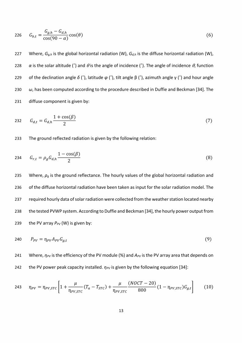
Where, Gg,h is the global horizontal radiation (W), Gd,h is the diffuse horizontal radiation (W), 227
α is the solar altitude (˚) and θ is the angle of incidence (˚). The angle of incidence θ, function 228
of the declination angle δ (˚), latitude φ (˚), tilt angle β (˚), azimuth angle γ (˚) and hour angle 229
ω, has been computed according to the procedure described in Duffie and Beckman [34]. The 230
diffuse component is given by: 231
, ,1 cos
2 7 232
The ground reflected radiation is given by the following relation: 233
, ,1 cos
2 8 234
Where, ρg is the ground reflectance. The hourly values of the global horizontal radiation and 235
of the diffuse horizontal radiation have been taken as input for the solar radiation model. The 236
required hourly data of solar radiation were collected from the weather station located nearby 237
the tested PVWP system. According to Duffie and Beckman [34], the hourly power output from 238
the PV array PPV (W) is given by: 239
ƞ , 9 240
Where, ƞPV is the efficiency of the PV module (%) and APV is the PV array area that depends on 241
the PV power peak capacity installed. ƞPV is given by the following equation [34]: 242
ƞ ƞ , 1ƞ , ƞ ,
20800
1 ƞ , , 10 243

14
Where, ƞPV,STC is the efficiency of the PV module at standard test conditions (STC), μ is the 244
temperature coefficient of the output power (%/°C), Ta is the ambient temperature (°C), TSTC 245
is the standard test conditions temperature (25°C) and NOCT is the nominal operating cell 246
temperature (°C). According to Duffie and Beckman [34], the temperature coefficient of the 247
output power μ can be approximated to: 248
ƞ , 11 249
Where, μVoc (V/°C) is the open circuit voltage temperature coefficient and Vmp (V) is the voltage 250
at maximum power point. Table 2 summarizes all the characteristic parameters of the PV 251
modules simulated in this paper. 252
253
254
255
256
257
258
259
260
261
262

15
Table 2: Characterizing parameters of the PV module (CEEG SST 160‐72P) [35]. 263
Imp (A) 4.6
Vmp (V) 34.8
Isc (A) 5.16
Voc (V) 43.8
Area (m²) 1.32
ηPV,STC (%) 12.56
μVoc (V/°C) ‐0.147
NOCT (°C) 45
3.2 Inverter‐water pumping system 264
The water pumped by a PVWP system significantly depends on the dynamic variability of the 265
solar radiation, ambient temperature, performances of the inverter and the pumping system. 266
Solar radiation and ambient temperature affect primarily the power output from the PV array 267
whereas the ambient temperature and the supplied power affect the efficiencies of the 268
inverter and pump. The efficiency of the inverter has been taken from an inverter database 269
and set to 95% [36]. The pump efficiency curve (water flow versus power input for a given 270
head) has been calculated from the standard characteristic pump curve (head versus water 271
flow) according to the following set of equations derived from the affinity laws and compiled 272
by Abella et al. [37]: 273
12 274

16
, ƞ 13 275
,
ƞ , ƞ 14 276
Where, Qo (m3/h) is the operational water flow corresponding to the operational hydraulic 277
head Ho (m), Qr is the reference water flow (m3/h) at the reference hydraulic head Hr (m) from 278
the pump standard characteristic curve, Pp,o is the operational pump power (W), ƞm,o is the 279
efficiency of the motor at the corresponding working conditions and ƞinv is the efficiency of 280
the inverter (%). 281
3.3 Irrigation water requirements 282
The assessment of the water demand plays a key role in the design of the PV array, pumping 283
unit and irrigation system. Moreover, the evaluation of the crop water requirements is 284
significant in order to guarantee a sustainable and efficient management of the water 285
resources, since the water demand cannot exceed the available water resources. The water 286
demand for the entire crop cycle is strictly bounded to the climatic conditions of the specific 287
site, especially air humidity, ambient temperature, solar radiation, wind speed and 288
precipitation. The crop water demand and yield response to water is typically determined 289
from the reference evapotranspiration ET0. The daily and hourly assessment of the crop water 290
demand has been evaluated using the FAO Penman‐Monteith method [38]. The hourly 291
reference evapotranspiration ET0 (mm/hour) is given by the following relationship: 292
0.408 37273
1 0.34 15 293

17
Where, Rn is the net radiation at the grass surface (MJ/m2 hour), G is the soil heat flux density 294
(MJ/m2 hour), Ta is the mean hourly air temperature (°C), Δ is the saturation slope of vapor 295
pressure curve at Ta (kPa/ °C), γ is the psychrometric constant expressed (kPa/°C), es is 296
saturation vapour pressure (kPa), ea is the average hourly actual vapour pressure (kPa) and u2 297
is the average hourly wind speed (m/s). The irrigation water requirements have been assessed 298
from the reference evapotranspiration ET0, calculating the evapotranspiration in cultural 299
conditions ETc, the effective precipitation Pe and taking into account the efficiency of the 300
irrigation system. The procedure to compute the irrigation water requirements is thoroughly 301
described in Campana et al. [15] and in Allen et al. [38]. 302
3.4 Crop growth model 303
To evaluate the benefits of PVWP systems, predicting the crop yield corresponding to the 304
water supply represents a key issue. In 1970s, FAO proposed a relationship between crop yield 305
and water supply to predict the reduction in crop yield. The crop‐water production function 306
relates the relative yield reduction to the relative reduction in evapotranspiration and is given 307
by Allen et al. [38]: 308
1 1 16 309
Where, Ya is the actual yield (tonne DM/ha), Ym is the maximum yield (tonne DM/ha), Ky is the 310
yield response factor, ETa is the actual evapotranspiration (mm/hour) and ETc is the 311
evapotranspiration in cultural conditions with no water stress (mm/hour). The actual yield Ya 312
represents the crop yield reduction compared to the maximum due to a reduction in the water 313
provided through irrigation. The maximum Alfalfa yield Ym used in the simulations has been 314
assumed equal to 8 tonne DM/ha year as confirmed by a local specialist of the studied area 315

18
[39]. The yield response factor Ky simplifies the complex natural procedures that rule the effect 316
of water deficit on the crop productivity. Ky for Alfalfa is equal to 1.1 as given by Allen et al. 317
[38]. The actual evapotranspiration ETa depends on the available water supply to the crop 318
(both through irrigation and rainfall) and on the soil parameters. The soil parameters assumed 319
in this work were taken from a previous work conducted in the same studied area [21]. The 320
procedure adopted to calculate the actual evapotranspiration ETa is thoroughly described in 321
Allen et al. [38]. Several papers have used the crop‐water production function for estimating 322
the crop productivity: Garg and Dadhich [40] used and validated the crop yield function for 323
assessing the effect of deficit irrigation on eight different crops in India; Igbadun et al. [41] 324
compared four different crop‐water production functions for evaluating the effect of deficit 325
irrigation on maize. It resulted that Equation 16 was the best for simulating the crop yield. In 326
this paper, the crop‐water production function has been used as direct method to simulate 327
the crop yield on the basis of the water supplied by the PVWP system. The crop yield 328
simulations together with the crop prices have been used to evaluate the revenues generated 329
by the PVWP system operation in order to identify the optimal point between revenues, costs 330
and constraints. 331
3.5 Groundwater supply model 332
The modelling of the aquifer response to the PVWP system operation is of significant 333
importance for predicting the drawdown s (the lowering of the water level in the well 334
compared to the static water level) and then the effective dynamic head of the pumping 335
system. During the operation of PVWP system, the drawdown s results in unsteady conditions 336
for most of the time due to the dynamic variation of the power output from the PV array. 337
Typically, groundwater transient modelling is based on Theis equation, which gives the 338

19
unsteady distribution of the drawdown s at a radial distance r and at the time t under the 339
following assumptions: (I) homogeneous and isotropic confined aquifer, (II) no source 340
recharging the aquifer, (III) aquifer compressible, (VI) water released instantaneously as the 341
head is lowered and (V) constant pumping flow [42]. The assumption regarding the constant 342
pumping is unrealistic for PVWP system application and make the Theis equation 343
inappropriate for groundwater flow modelling. The analytical solutions of the equations 344
governing groundwater flows assuming inconstant pumping flows were obtained by Ospina 345
et al. [43]. In this work, the method proposed by Rasmussen et al. [44] is used to simulate the 346
drawdown. If the pumped water and the characteristic of the aquifer are known, the following 347
equation calculates the drawdown s: 348
,2
17 349
Where, r is the distance from the pumping well assumed equal to 1 m, t is the time variable 350
(1h), Q0 is the pumping rate (m3/h), T is the aquifer transmissivity (m2/h), K0 is the zero‐order 351
modified Bessel function, i is the imaginary number, ω is the pumping frequency (given by the 352
ratio between 2π and p, the pumping cycle) (Hz) and D is the hydraulic diffusivity (m2/h). The 353
aquifer transmissivity and the hydraulic diffusivity were taken from the pumping tests carried 354
out by Zhang et al. [45]. 355
3.6 Model validation 356
To obtain the optimal results, it is of great importance to select the models that can simulate 357
the PVWP system accurately and provide correct inputs to the optimization. In the work 358
conducted by Glasnovic and Margeta [12], the models were not carefully validated. In this 359

20
work, measurements have been conducted at a pilot PVWP system and the models used in 360
optimization have been validated against the measurements. 361
Measurements at the pilot PVWP system 362
The tested PVWP system is located in the Wulanchabu desert grassland area, Inner Mongolia, 363
China, which latitude, longitude and altitude of the site are 41.32˚ N, 111.22˚ E and 1590 m 364
above the mean sea level. It is used to provide water for 1 ha of Alfalfa cultivated field. The 365
main system components and PV array orientation angles are listed in Table 3. 366
Table 3: PVWP system components and characteristics. 367
Number PV modules 9
PV power (kWp) 1.44
Pump (kW) 1.1 (AC centrifugal)
Tilt angle (°) 42
Azimuth (°) ‐36
368
To avoid dry running of the motor‐pump, a water level probe is installed on the upper part of 369
the pump. If the water level in the well reaches the probe, the inverter shuts down and makes 370
attempt to restart each 30 minutes. The well is marked out by a static water level of 5 m below 371
the ground surface. The pump is positioned at the bottom of the well, at 3.5 m depth from 372
the static water level. The pump safety probe is installed on the top of the pump, at 2.5 m 373
depth from the static water level. To measure the variation of the well water level, a water 374
pressure probe with data logger is installed at the bottom of the well. The PVWP system has 375
been tested in two different scenarios: recirculation scenario (S1) ‐ the water lifted up by the 376
pumping system was recirculated back into the well; and micro irrigation scenario (S2) ‐ the 377

21
water lifted up from the well is pumped directly into a micro irrigation system located about 378
150 m far from the well. S1 has aimed to test the pumping system and to validate the models 379
regarding the PVWP system. The main purpose of S2 was to analyse the effects of pumping 380
on the groundwater level. To measure the water pumped from the well, two flow meters are 381
installed along the pipeline network. All the performed measurements and the corresponding 382
used instruments are listed in Table 4. Figure 3 shows a schematic diagram of the tested PVWP 383
system scenarios together with the instruments used for gathering the operational data. 384
385
Table 4: Measurement carried out during the tests and the corresponding instruments and 386
resolutions. 387
Measurements Instrument Logging time Resolution
Solar radiation Pyranometer 1 hour ± 1 W/m2
Power DC/AC power meter 1 hour ± 1 W
Water flow Flowmeter 1 hour ± 0.001 m3
Well water table Pressure sensor 1 hour ± 0.02 mwc
Evapotranspiration Weighing lysimeter 1hour ± 0.02 mm
388
The measured data about solar radiation, power output and water flow were used to validate 389
the PVWP system model, in particular the pump efficiency curve (water flow versus power 390
input for a given head). The measurements of the well water level were used to validate the 391
model related to the groundwater level response to pumping. The weighing lysimeter data 392

22
were compared with the modelled data of evapotranspiration to validate the model used to 393
calculate the crop water demand. 394
395
Figure 3: Schematic diagram of the system configurations used during the tests. 396
397
It has to be pointed out that the tests carried out in irrigation scenario (S2) aimed to analyse 398
the effects of PVWP system operation on the groundwater level and to introduce the novel 399
optimization procedure for PVWP systems for irrigation. 400
PVWP models validation 401
Figure 4 compares the simulated results and the measured water flow. Good agreement is 402
observed at power inputs lower than 800 W. The discrepancy between modelled data and 403
measured data is higher at higher PV power inputs due to the system configuration: PVWP 404
23
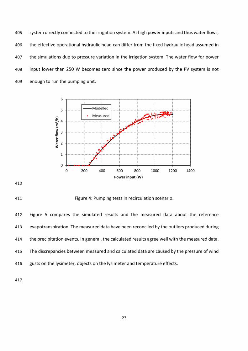
system directly connected to the irrigation system. At high power inputs and thus water flows, 405
the effective operational hydraulic head can differ from the fixed hydraulic head assumed in 406
the simulations due to pressure variation in the irrigation system. The water flow for power 407
input lower than 250 W becomes zero since the power produced by the PV system is not 408
enough to run the pumping unit. 409
410
Figure 4: Pumping tests in recirculation scenario. 411
Figure 5 compares the simulated results and the measured data about the reference 412
evapotranspiration. The measured data have been reconciled by the outliers produced during 413
the precipitation events. In general, the calculated results agree well with the measured data. 414
The discrepancies between measured and calculated data are caused by the pressure of wind 415
gusts on the lysimeter, objects on the lysimeter and temperature effects. 416
417
0
1
2
3
4
5
6
0 200 400 600 800 1000 1200 1400
Water flow (m³/h)
Power input (W)
Modelled
Measured

24
418
Figure 5: Measured and modelled hourly evapotranspiration data. 419
Figure 6 shows the modelled results and field measurements of the drawdown as a function 420
of the water flow. 421
422
Figure 6: Measured and modelled hourly groundwater level. 423
The discrepancy may be caused by the poor borehole construction technique, inadequate and 424
low accuracy instrumentation and field conditions. Nevertheless, it has to be pointed out that 425
0
0,05
0,1
0,15
0,2
0,25
0,3
0,35
0,4
0,45
0 10 20 30 40 50 60 70
Reference evapotran
spiration (mm/h)
Time (h)
Modelled
Measured
0
0,5
1
1,5
2
2,5
3
0 1 2 3 4 5
Drawdown (m)
Water flow (m³/h)
Modelled
Measured
25
the maximum deviation between measured and modelled data at the highest pumping rate is 426
less than 0.5 m. It implies that the model can be considered suitable to describe at least the 427
maximum pumping effect in terms of drawdown. Moreover, it has to be emphasized that the 428
same model showed an excellent agreement with the field measurement data in previous 429
tests carried out by Rasmussen et al. [44] at different aquifers with high accuracy equipment. 430
4 Optimization results and discussions 431
4.1 Identified problem 432
Figure 7 shows the measured pumped water as a function of the solar radiation and the water 433
level in the well. Since the pumped water by the PVWP system is larger than the recharge rate 434
of the well, the groundwater table declines. Therefore, it implies that the designed PVWP 435
system was oversized. To avoid dry‐up conditions, the inverter safety control system stops the 436
pump and the operation of the system is interrupted after 12 pm every half hour. Although 437
there is still abundant solar radiation and thus power from the PV array, the pumped water 438
volume decreases of about half. To overcome the encountered problem, it would have been 439
significant to test the recharge rate of well before the installation of the PVWP system. 440
Moreover, it has to be pointed out that the water availability in the well can notably vary from 441
year to year, especially from wet to dry year, affecting consequently the system design and 442
the irrigable area. 443
444
445

26
446
Figure 7: Pumping tests in irrigation scenario as function of the solar radiation and water 447
level in the well. 448
Another issue related to the operation of the studied PVWP system is the discrepancy 449
between crop water requirements and pumped water. The calculated monthly Alfalfa water 450
requirement varies a lot during the irrigation season registering its peak in June, as shown in 451
Fig 8. Comparing the modelled pumped water with the water demand, it is clear that the 452
PVWP system is unable to meet the irrigation water requirement for most of the irrigation 453
season. 454
455
0
200
400
600
800
1000
1200
0
1
2
3
4
5
6
6 8 10 12 14 16 18
Solar radiation (W/m
²)
Water flow (m³/h)
Well water level (m)
Time (h)
Water flow
Water table
Solar radiation

27
456
Figure 8: Alfalfa water demand, effective rainfall and pumped water from the existing PVWP 457
system. 458
On one hand the PVWP system is oversized since the water level in the well reach the bottom; 459
but on the other hand the PVWP system is also undersized since it cannot supply the crop 460
water need during the irrigation season. It has to be pointed out that the procedure adopted 461
to design the existing PVWP system is unknown and not led by the authors of this paper. 462
4.2 System optimization 463
Using the approach given in section 2.6, the existing system has been optimized assuming a 464
maximum hourly drawdown sh equal to 2.5 m that corresponds to the depth of the pump hp 465
measured from the static water level. Table 5 summarizes the characteristic parameters 466
(decision variables, operation failures, ICC, Alfalfa yield and PBP) for the existing and optimized 467
PVWP system. 468
469
470
0
10
20
30
40
50
60
70
80
90
Apr May Jun Jul
Crop water requirements (m³/ha day)
Pumped water (m
³/day)
Effective precipitation (mm)
Month
Crop water requirementsPumped water existing systemEffective precipitation

28
Table 5: Existing and optimized PVWP characteristic parameters. 471
Parameter Existing system Optimized system
Number PV modules 9 6
PVWP capacity (kWp) 1.44 0.96
Pump capacity (kW) 1.1 1.1
Tilt angle (°) 42 10
Azimuth (°) ‐36 8
ICC (US$) 4800 3900
Failures (time) 350 0
Ya (tonne DM/ha) 2.7 2.6
PBP (years) > lifetime (forage
price 207
$/tonne DM)
16 (forage price 207
$/tonne DM)
472
The constraint due to the decline of the groundwater level reduces the PVWP capacity. As a 473
result, the PV size is decreased from 1.44 kWp to 0.96 kWp. In addition, the optimization of the 474
tilt and azimuth angle allows an increase of 10% in the PV power output during the irrigation 475
season compared to the existing orientation. The optimal tilt angle maximize the solar 476
irradiation harvested by the PV array during the irrigation period between April and July. 477
Figure 9 shows the effect of tilt angle on the annual revenues Rann. 478

29
479
Figure 9: Effect of tilt angle on the annual revenues. 480
The optimal tilt angle causes an increase of the annual revenues of about 8% compared to the 481
tilt angle of the existing system. The ICC for the existing system is 4800 US$. The main cost 482
item is represented by the PV modules accounting for 60% of the ICC, followed by engineering 483
and installation costs and inverter representing a share of 17% and 14%, respectively. The ICC 484
for the optimized system is 3900 US$, corresponding to a reduction in the ICC of 18.8% 485
compared to the current PVWP system. The reduction in investment cost is mainly due to the 486
less investment in PV modules and inverter and the resulting reduction in project 487
implementation costs. 488
In addition, the continuous operation is guaranteed during the whole irrigation season. 489
Compared to the 350 times that the existing system is shut down to avoid dry‐up, the 490
optimized system never reaches the set level corresponding to the safety probe. Figure 10 491
shows the well water level trend for the optimized system during the irrigation season. 492
700
750
800
850
900
0 5 10 15 20 25 30 35 40
Ran
n($)
Tilt angle (°)

30
493
Figure 10: Well water level trend induced by the optimized system during the irrigation 494
season. 495
To clearly illustrate the operation difference between the existing system and the optimal 496
system, dynamic simulations were conducted with a time step of 10 minutes for two days in 497
June. Figure 11 and 12 show the results of water flow and well water level. The optimal system 498
operates between 8 am and 6 pm reaching an hourly maximum flow rate of about 3.9 m3/h 499
(0.65 m3/10 min) around 12pm, producing a maximum drawdown of 2.3 m (equivalent to a 500
minimum well water level of 1.2 m) without reaching the water level probe (installed at 1 501
meter depth). On the contrary, the existing system is shut down in every hour after 12pm. 502
0
0,5
1
1,5
2
2,5
3
3,5
4
0 400 800 1200 1600 2000 2400 2800
Well water level (m)
Time (hour)
Safety water level probe depth

31
503
Figure 11: Simulations of the pumped water and well water level for the existing and 504
optimized PVWP systems. 505
506
Figure 12: Simulations of the well water level for the existing and optimized PVWP systems. 507
Despite the decreased PV size, the effects of the pumped water on the crop yield in 508
insignificant due to the continuous shutdowns of the current installed PVWP system. The 509
resulting annual crop yields at the end of the irrigation season are 2.7 and 2.6 tonne DM/ha 510
0
0,1
0,2
0,3
0,4
0,5
0,6
0,7
0,8
0,9
1
0 4 8 12 16 20 0 4 8 12 16 20
Water flow (m³/10 m
in)
Time (h)
Existing PVWP systemOptimized PVWP system
0
0,5
1
1,5
2
2,5
3
3,5
4
0 4 8 12 16 20 0 4 8 12 16 20
Well water level (m)
Time (h)
Existing PVWP system
Optimized PVWP system

32
for the existing system and the optimized system, respectively. Since the save from the ICC of 511
PV is much larger, the optimized system has a shorter PBP and the optimization makes the 512
PVWP system more suitable. 513
4.3 Sensitivity study 514
Sensitivity studies have been conducted to understand the effect of crop price and PV module 515
price, which are the key parameters for the economic analysis, on the optimization results. 516
The forage price has been set to vary between 150 and 300 $/tonne DM, whereas the PV 517
module price has been varied between 1 and 2 $/Wp. 518
Figures 13 shows the effect of forage price on the optimal PVWP system capacity assuming a 519
constant PV module price of 1.5$/Wp together with the corresponding annual profit. With the 520
increase of forage price, the annual profit rises; however, the forage price doesn’t affect the 521
optimal PVWP system size clearly. Similarly, there is no obvious impact on the optimal PVWP 522
system capacity from the PV modules prices either, as depicted in Figure 14. The explanation 523
is that the groundwater constraint narrows the search of the optimal PVWP system capacity 524
into a small range: between 0.25 to 0.96 kWp (the lower threshold corresponds to the 525
minimum power peak to run the pumping system whereas the upper threshold corresponds 526
to the maximum power peak to avoid an excessive drawdown). The search of the optimal 527
PVWP system capacity is thus limited in a region where both the crop yield, and thus the 528
annual revenues, and the PVWP system cost functions have a linear trend. Accordingly, the 529
effects of PV module and forage price variation have a negligible effect in the search of the 530
optimal system size. 531

33
532
Figure 13: Effect of forage price on the optimal PVWP system size and annual revenues 533
assuming a constant PV module price of 1.5$/Wp. 534
535
Figure 14: Effect of PV module price on the optimal PVWP system capacity assuming a 536
constant forage price of 200 $/tonne DM. 537
As an example, Figure 15 shows the effect of the groundwater level constraint and PV module 538
price on the maximization of the annual profit, assuming a constant forage price of 539
0
100
200
300
400
0,7
0,8
0,9
1
1,1
100 150 200 250 300 350
Annual profit ($)
Optimal PVWP cap
acity (kW
p)
Forage price ($/tonne DM)
Optimal PVWP capacity
Annual profit
0,94
0,95
0,96
0,97
0,98
0,75 1 1,25 1,5 1,75 2 2,25
Optimal PVWP cap
acity (kW
p)
PV module price ($/Wp)
Optimal PVWP capacity

34
150$/tonne DM. If the ground water constraint is taken into account, the optimal PVWP 540
system capacity that maximizes the annual profit is 0.96 kWp, independently from the PV 541
module price. Nevertheless, if the groundwater level constraint is disregarded, since the 542
relationship between PVWP system capacity and crop yield is nonlinear, the price of PV 543
modules has more obvious impacts on the optimal PVWP system capacity that maximizes the 544
annual profit (2 and 2.2 kWp for PV module price of 2.0 and 1.0 $/Wp, respectively). 545
546
Figure 15: Effect of the groundwater level constraint on the optimal PVWP system capacity. 547
548
To identify those effects, the same sensitivity analyses have been conducted without the 549
constraint of the groundwater level. Results are shown in Figure 16. The variation of PV 550
modules and forage prices result in opposite trends. The increase of the forage price intends 551
‐200
0
200
400
600
800
0,4 0,6 0,8 1 1,2 1,4 1,6 1,8 2 2,2 2,4 2,6
Annual profit ($)
PVWP capacity (kWp)
PV module 1.0 $/Wp
PV module 2.0 $/Wp
Groundwater level constraint

35
to raise the PVWP capacity; while the increase of PV price intends to reduce the capacity. The 552
effect of the sensitive parameters variation on the PVWP system capacity is about 10%. The 553
results show the effectiveness and importance of considering the economic aspects into the 554
optimization of PVWP systems for irrigation, especially for large applications where the 555
optimization design can lead to significant economic benefits. 556
557
Figure 16: Effect of forage price and PV module price on the optimal PVWP system size 558
assuming no groundwater response constraint. 559
The groundwater level constraint has played the key role in determining the optimal size of the PVWP 560
system, assuming no system failures during the irrigation season (maximum reliability of the PVWP 561
system in terms of operation continuity). The PV modules and forage price can affect the optimal PVWP 562
system size but only if the drawdown is not a limiting factor. The optimization and simulation results 563
show also how the groundwater level constraint is significant for ensuring high crop productivity and 564
thus high PVWP system profitability. 565
100 150 200 250 300 350 400
2
2,02
2,04
2,06
2,08
2,1
2,12
2,14
2,16
2
2,02
2,04
2,06
2,08
2,1
2,12
2,14
2,16
0,75 1 1,25 1,5 1,75 2 2,25
Forage price ($/tonne DM)
Optimal PVWP cap
acity (kW
p)
PV module price ($/Wp)
Optimal PVWP capacity=f(PV module price)
Optimal PVWP capacity=f(Forage price)

36
5 Conclusions 566
A new approach to optimize the photovoltaic water pumping (PVWP) system for irrigation has 567
been proposed with the consideration of groundwater response and economic factors in this 568
paper. Applying the proposed approach to an existing system shows a reduction in PV module 569
size (from 1.44 down to 0.96 kWp). This implies a decrease of 18.8% in the investment capital 570
cost and therefore improve the economic feasibility of PVWP clearly. Even though the prices 571
of crop and PV modules are the key parameters concerning the economic feasibility, according 572
to the sensitivity study, they don’t have clearly effects on the optimal system capacity if the 573
ground water level is limited. However, if the groundwater level response to pumping does 574
not represent a constraint, the increase of the forage price intends to raise the PVWP capacity; 575
while the increase of PV price intend to reduce it. 576
Acknowledgments 577
The authors are grateful to the Swedish International Development Cooperation Agency 578
(SIDA) and Swedish Agency for Economic and Regional Growth (Tillväxtverket) for the financial 579
support. 580
References 581
[1] Longjun C., “UN Convention to combat desertification”, Encyclopedia of Environmental 582
Health, 2011, DOI: http://dx.doi.org/10.1016/B978‐0‐444‐52272‐6.00654‐1. 583
[2] Yan J., Gao Z. Wang H. Liu J., “Qinghai pasture conservation using solar photovoltaic (PV)‐584
driven irrigation”, Asian Development Bank, Project Report, 2010. 585
37
[3] Bouzidi B., Haddadi M., Belmokhtar O., “Assessment of a photovoltaic pumping system in 586
the areas of the Algerian Sahara”, Renewable and Sustainable Energy Reviews 13 (2009) 879–587
886. 588
[4] Hrayshat E.S., Al‐Soud M.S., “Potential of solar energy development for water pumping in 589
Jordan”, Renewable Energy 29 (2004) 1393–1399. 590
[5] Bouzidi B., “Viability of solar or wind for water pumping systems in the Algerian Sahara 591
regions – case study Adrar”, Renewable and Sustainable Energy Reviews 15 (2011) 4436– 592
4442. 593
[6] Ghoneim A.A., “Design optimization of photovoltaic powered water pumping systems”, 594
Energy Conversion and Management 47 (2006) 1449–1463. 595
[7] Benghanem M., Daffallah K.O., Alamri S.N., Joraid A.A., “Effect of pumping head on solar 596
water pumping system”, Energy Conversion and Management 77 (2014) 334–339. 597
[8] Mokeddem A., Midoun A., Kadri D., Hiadsi S., Raja I.A., “Performance of a directly‐coupled 598
PV water pumping system”, Energy Conversion and Management 52 (2011) 3089–3095. 599
[9] Boutelhig A., Hadjarab A., Bakelli Y., “Comparison study to select an optimum photovoltaic 600
pumping system (PVPS) configuration upon experimental performances data of two different 601
dc pumps tested at Ghardaïa site”, Energy Procedia 6 (2011) 769–776. 602
[10] Hamidat A., Benyoucef B., Hartani T., “Small‐scale irrigation with photovoltaic water 603
pumping system in Sahara regions”, Renewable Energy 28 (2003) 1081–1096. 604
[11] Senol R., “An analysis of solar energy and irrigation systems in Turkey”, Energy Policy 47 605
(2012) 478–486. 606
[12] Glasnovic Z., Margeta J., “A model for optimal sizing of photovoltaic irrigation water 607
pumping systems”, Solar Energy 81 (2007) 904–916. 608

38
[13] Pande P.C., Singh A.K., Ansari S., Vyas S.K., Dave B.K., “Design development and testing of 609
a solar PV pump based drip system for orchards”, Renewable Energy 28 (2003) 385–396. 610
[14] Ould‐Amrouche S., Rekioua D., Hamidat A., “Modelling photovoltaic water pumping 611
systems and evaluation of their CO2 emissions mitigation potential”, Applied Energy 87 (2010) 612
3451–3459. 613
[15] Campana P.E., Li H., Yan J., “Dynamic modelling of a PV pumping system with special 614
consideration on water demand”, Applied Energy 112 (2013) 635–645. 615
[16] Amer E.H., Younes M.A., “Estimating the monthly discharge of a photovoltaic water 616
pumping system: Model verification”, Energy Conversion and Management 47 (2006) 2092–617
2102. 618
[17] Hamidat A., Benyoucef B., “Mathematic models of photovoltaic motor‐pump systems”, 619
Renewable Energy 33 (2008) 933–942. 620
[18] Luo Y., Sophocleous M., “Seasonal groundwater contribution to crop‐water use assessed 621
with lysimeter observations and model simulations”, Journal of Hydrology 389 (2010) 325–622
335. 623
[19] Campana P.E., Zhu Y., Brugiati E., Li H., Yan J., “PV water pumping for irrigation equipped 624
with a novel control system for water savings”, Proceedings of the 6th International 625
Conference on Applied Energy ‐ ICAE2014. 626
[20] Campana P.E. Olsson A., Zhang C., Berretta S., Li H., Yan J., “On‐grid photovoltaic water 627
pumping systems for agricultural purposes: comparison of the potential benefits under three 628
different incentive schemes”, Proceedings of the 13th World Renewable Energy Congress ‐ 629
WREC XIII. 630

39
[21] Xu H., Liu J., Qin D., Gao X., Yan J., “Feasibility analysis of solar irrigation system for 631
pastures conservation in a demonstration area in Inner Mongolia”, Applied Energy 112 (2013) 632
697–702. 633
[22] Yu Y., Liu J., Wang H., Liu M., “Assess the potential of solar irrigation systems for sustaining 634
pasture lands in arid regions – A case study in Northwestern China”, Applied Energy 88 (2011) 635
3176–3182. 636
[23] Gao X., Liu J., Zhang J., Yan J., Bao S., Xua H., Qin T., “Feasibility evaluation of solar 637
photovoltaic pumping irrigation system based on analysis of dynamic variation of 638
groundwater table”, Applied Energy 105 (2013) 182–193. 639
[24] Gao T., Zhang R., Zhang J., “Effect of Irrigation on Vegetation Production and Biodiversity 640
on Grassland”, Procedia Engineering 00 (2011) 000–0003– 616. 641
[25] Olsson A., Campana P.E., Lind M., Yan J., “Potential for carbon sequestration and 642
mitigation of climate change by irrigation of grasslands”, Applied Energy 136 (2014) 1145–643
1154. 644
[26] Olsson A., Lind M., Yan J., “PV water pumping for increased resilience in dry land 645
agriculture”, Proceedings of the 6th International Conference on Applied Energy ‐ ICAE2014. 646
[27] Zhang C., Yan J., “Business model innovation on the photovoltaic water pumping systems 647
for grassland and farmland conservation in China”, Proceedings of the 6th International 648
Conference on Applied Energy ‐ ICAE2014. 649
[28] Merei G., Berger C., Sauer D.U., “Optimization of an off‐grid hybrid PV–Wind–Diesel 650
system with different battery technologies using genetic algorithm”, Solar Energy 97 (2013) 651
460–473. 652

40
[29] Bean R., Wilhelm J., “U.S. Alfalfa Exports to China Continue Rapid Growth”, USDA Foreign 653
Agricultural Service‐Global Agricultural Information Network Report, 2011. 654
[30] The World Bank. Available at: http://data.worldbank.org/indicator/FR.INR.RINR. 655
Accessed: 1st July 2014. 656
[31] Solartech. Available at: http://www.solartech.cn. Accessed: 1st July 2014. 657
[32] Campana P.E., Olsson A., Li H., Yan J., “An economic analysis of photovoltaic water 658
pumping irrigation systems”, International Journal of Green Energy, (2015) (In press). 659
[33] SolveXL. Available at: http://www.solvexl.com/. Accessed: 1st July 2014. 660
[34] Duffie J.A., Beckman W.A., “Solar engineering of thermal processes”, 3rd ed. Wiley; 2006. 661
[35] CEEG. Available at: http://www.ceeg.cn/English/?lang=2. Accessed: 1st July 2014. 662
[36] PVsyst. Available at: http://www.pvsyst.com/en/. Accessed: 1st July 2014. 663
[37] Abella M.A., Lorenzo E., Chenlo F., “PV water pumping systems based on standard 664
frequency converters”, Prog. Photovolt: Res. Appl. 2003; 11:179–191 (DOI: 10.1002/pip.475). 665
[38] Allen R.G., Pereira L.S., Raes D., Smith M., “Crop evapotranspiration. Guidelines for 666
computing crop water requirements”, FAO, 1998. 667
[39] Zhang, R. 2013. Personal communication. Institute of Water Resources for Pastoral Areas, 668
Hohhot, China. 669
[40] Garg N.K., Dadhich S.M., “A proposed method to determine yield response factors of 670
different crops under deficit irrigation using inverse formulation approach”, Agricultural 671
Water Management 137 (2014) 68–74. 672
[41] Igbadun H.E., Tarimo A.K.P.R., Salim B.A., Mahoo H.F., “Evaluation of selected crop water 673
production functions for an irrigated maize crop”, Agricultural water management 94 (2007) 674
1–10. 675

41
[42] Kruseman G.P., “Analysis and evaluation of pumping test data”, 2nd ed., ILRI, 1994. 676
[43] Ospina J., Guarin N., Velez M., “Analytical solutions for confined aquifers with non‐677
constant pumping using computer algebra”, Proceedings of the 2006 IASME/WSEAS Int. Conf. 678
on Water Resources, Hydraulics & Hydrology, Chalkida, Greece, May 11‐13, 2006 (pp7‐12). 679
[44] Rasmussen T.C., Haborak K.G., Young M.H., “Estimating aquifer hydraulic properties using 680
sinusoidal pumping at the Savannah River site, South Carolina, USA”, Hydrogeology Journal 681
(2003) 11:466–482. 682
[45] Zhang J., Liu J., Campana P.E., Zhang R., Yan J., Gao X., “Model of evapotranspiration and 683
groundwater level based on photovoltaic water pumping system”, Applied Energy 136 (2014) 684
1132–1137. 685
686