Embed Size (px)
Citation preview
1
Economic Policy, Political Accountability and the Room to Maneuver∗
Thomas Sattler ETH Zurich
Center for Comparative and International Studies Weinbergstrasse 11
8092 Zurich, Switzerland E-mail: [email protected]
Patrick T. Brandt University of Texas at Dallas School of Economic, Political
and Policy Sciences P.O Box 830688
Richardson, TX 75083 E-mail: [email protected]
John R. Freeman University of Minnesota Department of Political
Science 267 19th Avenue South Minneapolis, MN 55455
E-mail: [email protected]
January 20, 2006
ABSTRACT Most political scientists agree that governments retain substantial room to maneuver despite economic globalization. But these researchers assert rather than demonstrate that citizens are satisfied with economic policies and outcomes. We use a Bayesian multivariate time-series framework that allows us to analyze the dynamic relationship between popular evaluations of policymakers’ performance, government policy choices and macroeconomic outcomes in Britain from 1984 to 2006. Our results do not support the room to maneuver thesis. The British government was responsive to changes in political evaluations. Citizens then rewarded the government for its reaction with higher political support. However, the impact of government policy adjustments on inflation and economic growth was negligible. Government capacity to shape macroeconomic outcomes thus was limited. The results also show that before the central Bank of England was granted independence in 1997, the government used both monetary and fiscal policy in response to changes in popular evaluations. After 1997, the political influence over monetary policy decreased significantly and fiscal policy became the main economic policy instrument of the elected government.
∗ Paper prepared for presentation at the Conference on the Political Economy of International Finance, Federal Reserve Bank Atlanta, February 9, 2007. Brandt's and Freeman's research is sponsored by the National Science Foundation under grants numbers SES-0351179, SES-0351205 and SES-0540816. Sattler’s research is supported by the Swiss National Science Foundation under grant number 101412-962. The authors are solely responsible for the contents.
2
1. Introduction
Most political scientists agree that governments still retain substantial room to maneuver
in economically open democracies. Despite economic integration, tax rates and public sector
sizes have not been converging across advanced industrialized countries. Some scholars even find
a positive relationship between financial openness and government activity. From these findings,
researchers conclude that economic globalization has not constrained economic policymaking as
predicted by earlier, more pessimistic scholars.
These political scientists imply that citizens are satisfied with economic policies and
macroeconomic outcomes. Through voting and other forms of political participation, citizens
evaluate these policies and hold governments accountable for their choices. Economic
policymakers therefore use this room to implement the policies that citizens desire and to
generate the economic outcomes that are in the interest of the public.
This research assumes rather than demonstrates that citizens are satisfied with policies and
outcomes. It omits channels for popular preferences to feed back into policies and outcomes, and
does not explicitly analyze the connections between citizens’ evaluations of economic outcomes,
government policies and macroeconomic developments. Extant research only examines parts of
the causal nexus between popular evaluations, policies, and macroeconomic outcomes that
represent political accountability. Moreover, these studies fail to draw distinctions between short-
and long-term consequences of policy choices and to provide any estimates of the magnitudes
and durations of policy outcomes. Without sound estimates of these outcomes, we have no idea
how much, if any, room to maneuver democratic governments actually retain.
A complete analysis of room to maneuver requires that we uncover the causal chains that
connect political evaluations to policies to outcomes and then back to evaluations, as presented in
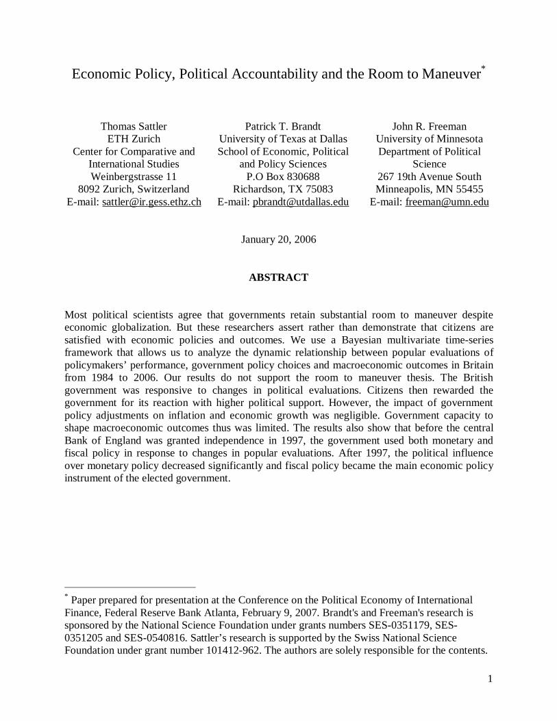
Figure 1. We have to show that governments not only have the capacity to resist market forces
and manage their macroeconomies, but also that publics are satisfied with the policy choices of
their governments. Only if governments are able to generate distinct economic outcomes that
reflect the preferences of their publics will room to maneuver exist. Room to maneuver means
that governments adjust economic policies when the public becomes increasingly dissatisfied
with economic policies, that the new policies have a strong and lasting effect on the
macroeconomy, and that citizens, in turn, appreciate the improvement in their well being.
3
Figure 1: Political Accountability in Economic Policy
To establish the degree of accountability that exists in contemporary democracies, we
need a new framework that accounts for the dynamic and simultaneous evolution of the key
economic and political variables. Existing models are incomplete because they treat the polity or
the economy as exogenous. Political scientists demonstrate the importance of economic factors
for popular evaluations and government approval. But they ignore how the government’s reaction
to changes in popular evaluations feed back into economic outcomes. Economists analyze how
monetary and fiscal policy affects the macroeconomy, but make no provisions for political
accountability. The political and economic literatures thus only analyze one side of the complete
political economy model in Figure 1.
We develop a political economy framework that allows for endogeneity between the open
economy and the macropolity. It fully accounts for the relationships between political and
economic forces without imposing strong restrictions about the underlying causal mechanism, as
is the case in standard political economy models. The model is interdisciplinary, combining
current research from political science, political economy and new open macroeconomics to
identify the model. We test our competing arguments about the existence of political
accountability using Bayesian structural time series methods for monthly data from 1984 to 2006
for the United Kingdom. The British economy has been highly open to trade and financial flows
and is characterized by a high degree of clarity of responsibility. It thus is a critical case because
if political accountability exists anywhere, we should find it in Britain. Our analysis splits the
data into two periods, 1984-1997 (a Tory period) and 1997-2006 (a Labour period) to evaluate
differences in accountability due to public preferences, economic policies and central bank
independence.
4
We find only limited evidence that accountability exists in open democracies. The British
government was responsive to changes in political evaluations. For instance, when sociotropic
economic expectations decrease, government debt increases which indicates higher fiscal
spending. Similarly, when personal economic expectations decline, the government lowers
interest rates. These policy choices fed back into popular evaluations, e.g. vote intentions. A
visible link form popular evaluations to policy and back to popular evaluations existed. This
accountability mechanism has only a small effect on the real economy. Although prices and
output respond to fiscal and monetary policy, the impact of policy on real economic outcomes is
tiny. This suggests that government capacity to shape macroeconomic outcomes in Britain was
limited and popular influence over economic policy had little effects.
Our results also show that policymaking differed considerably before and after the central
bank was granted independence. Fiscal policy was significantly more reactive to changes in
political evaluations after 1997 when the government did not control monetary policy. As regards
pre-election or “electorally induced cycles,” the results for the Tory period support Clark and
Hallerberg (2000) and contradict O'Mahony (2006); under mostly flexible exchange rates and
central bank dependence, there is evidence of pre-election effects in monetary policy only.
Mahoney’s results are partially supported by a pre-election fiscal policy effect in the Labour
period. Contrary to the predictions of Clark and Hallerberg, we also find pre-electoral monetary
effects in this period of flexible exchange rates and an independent central bank. Finally, we find
a number of anomalies that are inconsistent with theoretical expectations. Future research will
examine further these findings.
2. Policy Effectiveness and Accountability in Open Economies
2.1 Monetary Policy
Research from new open macroeconomics yields ambiguous conclusions about the room
to maneuver and accountability. Dynamic stochastic general equilibrium models with market
rigidities (e.g., inflexible prices, sticky wages and monopolistic competition) propose that
monetary policy can have a strong effect on economic output (Galí 2003; Galí and Monacelli
2005). The extensions of these theoretical models to open economies imply that an unexpected
5
monetary expansion may even increase both domestic and foreign output (Obstfeld and Rogoff
1995).1 Empirical studies show that domestic monetary contractions in fact have international
effects, e.g. lead to increases in nominal and real exchange rates (Clarida and Galí 1994;
Cushman and Zha 1997; Eichenbaum and Evans 1995). The effect on output is more ambiguous.
While some researchers find a considerable effect of a monetary shock on domestic and foreign
output (Betts and Devereux 2001; Kim 2001), others find that this effect is rather small
(Cushman and Zha 1997).
Based on insights from the Mundell-Fleming model, political scientists argue that despite
capital mobility, governments can use monetary policy to satisfy the demands from its
constituents. When the exchange rate is flexible, monetary expansions in an open economy lead
to currency depreciation. This depreciation stimulates exports that in turn benefit businesses and
workers in the trade sector (Frieden, 1991). Political scientists also contend that governments in
open economies with flexible exchange rates use monetary policy to create pre-election growth
spurts above the natural level, but only when the central bank is not independent (Clark and
Hallerberg 2000). Those governments that have not delegated monetary policy to an independent
central bank thus should be able to produce macroeconomic outcomes desired by their
constituents, at least in the short and medium runs.
If monetary policy is as effective as some of these results suggest, political accountability
should still exist in economically open democracies. We should observe a causal chain that
connects popular evaluations of economic outcomes to monetary policy choices, to
macroeconomic outcomes and back to popular evaluations. None of these studies explicitly 1 To what degree both countries benefit from the domestic monetary expansion depends on the
degree of exchange rate pass-through. When pass-through is large, i.e. when producers set prices
in the home currency, the exchange rate drops after a monetary expansion and shifts world
demand towards domestic products. Both countries benefit from the monetary expansion,
however, because the shock generally increases world demand (Obstfeld and Rogoff 1995).
When pass-through is small, i.e. when producers set prices in the purchasers’ currency, exchange
rate depreciations do not change relative prices of domestic and foreign products, but increase the
domestic currency value of revenues from exports. In such a pricing-to-market model, an
unexpected domestic monetary expansion can have adverse effects on foreign welfare because it
alters the foreign country’s terms of trade (Betts and Devereux 2000).
6
analyzes this complete relationship that connotes political accountability. They assume rather
than demonstrate the citizens are satisfied with economic policies and the resulting outcomes. To
show that room to maneuver and therefore accountability continues to exist in open economies, it
is necessary to establish that the complete connection between citizens’ evaluations, policy
choices and economic outcomes exists. Moreover, this has to be done for both non-electoral and
electoral periods. We can not simply assume, as Clark and Hallerberg (2000: 325) do, that in
non-electoral periods the preferences of the central bank and the government are identical, let
alone that citizens believe in and are satisfied with the natural rate of growth.2
In a previous study, we construct a political economy model that allows for such a test
(Sattler et al. 2006). We analyzed whether accountability in monetary policy existed in Britain
from 1981 to 1997 before the Bank of England was granted independence. Our results did not
support the room to maneuver thesis. The British government was responsive to changes in
political evaluations, and its policy choices effectively fed back into popular evaluations of
government policy. Hence, a visible link from popular evaluations to policy and back to popular
evaluations existed. However, this accountability mechanism worked outside the real economy.
The changes in monetary policy induced by shifts in popular evaluations had no impact on
inflation and economic growth. Government capacity to shape macroeconomic outcomes was
limited, and popular influence over monetary policy was ineffectual.
2.2 Fiscal Policy
2.2.1 Race to the Bottom
It is possible that governments primarily use fiscal rather than monetary policy to
influence economic developments and welfare, a possibility that our previous work does not take
into account. The propositions in the literature about room to maneuver and therefore
accountability in fiscal policy are quite contradictory.
Several scholars suggest that government’s room to pursue an autonomous fiscal policy is
highly constrained when countries become increasingly open to trade and capital flows. In their 2 Clark and Hallerberg assume that in non-electoral periods the central bank and government—
and, by implication, their citizens—prefer both the natural rate of growth and zero inflation.
7
view, increasing capital mobility and failure of governments to coordinate economic policies
inevitably decreases levels of taxation on mobile assets (e.g., Tanzi 1996). Countries with higher
taxation on capital experience a capital outflow to countries with lower taxation. Tax income
from capital investments then decrease dramatically when a country loses large amounts of
capital. Moreover, the decreasing level of investment leads to lower economic growth, lower
government receipts and hence lower public spending.
This situation leads to a ‘race to the bottom’ in taxation and government spending. A
country can increase its tax income initially if it lowers taxes slightly below the level of the other
countries that compete for capital. Mobile capital then flows to this low-taxation country, but
leads to an erosion of the tax base of the other countries that experience a capital outflow. These
countries then cut taxes below the level of the country with the lowest taxes to attract capital from
the other countries, and so on. When countries fail to coordinate their tax policies, the result is a
decrease in government receipts and lower public spending in all economically open countries.
A few recent studies take a more nuanced view, but their conclusions are similar. They
find that such a race to the bottom has not occurred, but capital mobility still restricts government
policy autonomy in serious ways. It prevents governments from increasing taxes in response to
higher spending requirements and from lowering taxes on immobile factors, such as labor, in
response to rising unemployment (Bretschger and Hettich 2002; 2005; Genschel 2002). The
government thus is trapped between the demands of business and voters. Citizens demand higher
government spending to cushion the adverse domestic economic and social effects of economic
integration. Capital owners request lower tax rates and threaten that they will move to other
countries if the government raises taxes to finance increased government spending.
This critical view suggests that accountability in fiscal policy does not exist in open
democracies. On the one hand, economic globalization causes structural changes and citizens
demand greater government involvement. On the other hand, constraints on fiscal policy that
result from capital mobility prevent policymakers from satisfying these requests. Lower tax
revenues force governments to cut social welfare expenditures, and the size of the public sector in
general tends to decrease. This causal chain implies that we should not observe a fiscal policy
change when citizens become increasingly dissatisfied with economic developments. Moreover,
there is no empirically observable effect from fiscal policy on real domestic economic outcomes.
8
2.2.2 Effective Fiscal Policy
Most political science scholars today challenge this pessimistic view. Empirical studies
show that despite economic integration, tax rates and public sectors sizes have not been
converging across advanced industrialized countries. Although there is some indication that
taxation of mobile capital decreased slightly, the extent of these changes is rather small (see also
Bearce forthcoming; Swank and Steinmo 2002). Some even find a positive relationship between
financial openness and tax rates (Garrett and Mitchell 2001; Quinn 1997). Similarly, researchers
find no evidence that public spending is declining (Bernauer and Achini 2000) or that there are
higher levels of public expenditures when international economic integration increases (Garrett
1998a; 1998b; Rodrik 1998). From these findings, political scientists conclude that governments
retain a significant degree of control over economic outcomes and social welfare in an
economically integrated world. This is particularly true when a single party enjoys a legislative
majority and decides to delegate fiscal policy to a minister or when a coalition of parties
negotiates spending targets upon its formation (Hallerberg and Von Hagen 1999).
Some models even suggest that under specific circumstances, fiscal policy is more
effective in an open than in a closed economy. Frieden (1991) argues that fiscal policy is
particularly effective when the economy is open and the exchange rate is fixed. In a closed
economy, excessive government spending leads to higher interest rates which reduce the impact
of fiscal policy on economic growth. In an open economy, however, interest rates are set globally
and remain stable because international investors buy government bonds to finance increased
government spending. If the exchange rate was flexible, its appreciation following this capital
inflow would reduce the impact of fiscal policy on economic growth. But since the exchange rate
is fixed, this is not the case. In an empirical analysis, Clark and Hallerberg (2000) find that
governments with fixed exchange rates use fiscal rather than monetary policy to stimulate the
economy before elections. O'Mahony (2006) revises these results and accounts for the absence of
full capital mobility, fiscal effects on prices, and trade openness. Her model predicts pre-
electoral cycles when exchange rates are flexible and an economy is open to trade flows.3 3 Contrary to Clark and Hallerberg (2000, Table 2), O'Mahony (2006) argues that if an economy
is open to trade and capital is only partially mobile, pre-election fiscal cycles can occur regardless
of whether the central bank is or is not independent.
9
These studies suggest that governments satisfy the demands of citizens to cushion the
adverse economic outcomes in open economies. When voters are increasingly dissatisfied with
macroeconomic developments, governments uses fiscal policy to influence economic outcomes.
Fiscal policy is an effective instrument and has a significant and sustained impact on the real
economy. Citizens then observe the government’s reaction and its positive effect on the economy.
Political evaluations of government policy and the resulting outcomes improve. In this case,
political accountability exists and works through fiscal policy.
But, insofar as political accountability is concerned, these are assertions not
demonstrations. None of these models includes any equations for citizens’ evaluations of
macroeconomic outcomes and policies, let alone for any feedback from these evaluations to
policymaking.
2.3 Institutions and the Connection Between Monetary and Fiscal Policy
As indicated in our discussion on monetary policy, central bank independence limits the
government’s ability to react to popular evaluations. Since most central banks in the
industrialized world have been granted independence during recent decades, the accountability
mechanisms, if they exist, may have changed. When a central bank is not autonomous, the
government can use both fiscal and monetary policy to influence economic developments. When
the government learns that citizens are dissatisfied with economic policies and outcomes, it can
lower interest rates and increase government spending to stimulate the economy. Fiscal and
monetary policies then are consistent and reinforce each other. The government’s reaction to
declines in popular evaluations effectively changes real economic outcomes. Citizens presumably
observe the policy change and its effects on economic developments and reward the government
with higher political support.
When technocratic central bankers control monetary policy, this possible accountability
mechanism should be weaker; it may even disappear. Monetary policymakers who do not depend
directly on the public support will be less responsive to political evaluations of policymaking.
Although delegation of monetary policy to an independent central bank helps solve the “time-
consistency problem” and hence enhances economic efficiency, the public loses control over an
important policy instrument. Our previous research shows that monetary policy played a

10
significant role for accountability in Britain before the Bank of England was granted
independence in 1997 (Sattler et al. 2006). Although the government’s capacity to shape real
economic outcomes was low, the Bank lowered interest rates when national economic
expectations of citizens became more pessimistic. We can expect that this link between political
evaluations and monetary policy weakens or breaks completely when monetary policy is
insulated from public control.
Besides its effect on monetary policy, central bank independence may also reduce fiscal
policy accountability. Monetary policy by a central bank exclusively focused on price stability
may reduce the effectiveness of fiscal policy. When the government increases the budget deficit
to satisfy the demands from voters with higher spending, the conservative central bank tightens
monetary policy to fight inflationary expectations. This contractionary monetary policy reduces
economic growth and thus diminishes fiscal policy effectiveness. Accountability in economic
policy then is limited because the government’s capacity to react to changes in political
evaluations is reduced.4
On the positive side, unexpected monetary shocks may be more effective when a
conservative central bank controls monetary policy. As our previous research shows, monetary
policy was essentially ineffective in Britain before the Bank of England became independent in
1997 (Sattler et al. 2006). Monetary policy effectiveness may be greater after 1997 because
central banks that are insulated from political pressure usually have a longer time horizon and
therefore enjoy greater low-inflation credibility than non-independent banks (Rogoff 1985;
Franzese 1999). When the monetary authority enjoys substantial monetary credibility,
unexpected policy interventions are likely to be more effective. With an autonomous central
bank, wage setters expect that inflation will be low in the future and set wages accordingly. An
4 Exemplary analyses of the connection between monetary and fiscal policy are Dixit and
Lambertini (2000; 2003). Note that these studies make no provision for popular evaluation of
monetary and fiscal policies (equilibria). The preferences of Dixit and Lambertini’s strategic
actors—the central bank and government fiscal authority—do not depend on the public’s
evaluations of the macroeconomy.
11
unexpected monetary expansion thus can have a strong effect on economic growth when wages
are inflexible in the short run.5
Although central bank officials usually cannot be held as directly accountable as their
fiscal counterparts, monetary policy by an independent central bank may better represent the
interests of the public than policy by a non-independent bank. If central bankers do not focus
exclusively on price stability, but also take into account the public’s evaluations of monetary
policy, central bank independence may increase accountability as we define it.6 When the citizens
become dissatisfied with economic developments, central bank interventions can effectively
affect the real economy. Citizens then observe these policy changes and the resulting economic
outcomes and subjective economic expectations become more optimistic.
If this form of accountability exists, we should observe that monetary policy reacts to
changes in subjective economic expectations, and these policy changes have a significant impact
on the real economy. Other indicators of political evaluations, however, do not play a significant
role in this accountability mechanism. Monetary policy should not react to changes in vote
intentions or prime minister approval since these forms of evaluations are irrelevant for the
independent central bank. Similarly, the elected government should get little or no credit for
monetary policy choices and economic conditions since it is not responsible for them.
2.4 Competing Models of Accountability
We represent the preceding arguments as two different models of economically open
democracies. The position that room to maneuver diminishes or even disappears when countries
become increasingly integrated into the world economy implies that no political accountability 5 The expectations-enhanced Philips’ curve represents the inverse relationship between growth
and inflationary expectations. For a theoretical derivation of this Philips’ curve from a dynamic
stochastic general equilibrium model, see Galí and Monacelli (2005). 6 There is evidence that independent central banks are interested in citizen’s evaluations of their
work. After a 1997 Treasury Committee Report on Central Bank accountability, the BoE began a
survey of the public’s understanding of its activities and of how well it is doing in the public
mind (Bank of England, Quarterly Bulletins, Summer 2001: 164-168; Summer 2003: 228-234).
On the governments’ central bank accountability studies see Leeper and Sterne (2002).
12
exists. In our “No Accountability” model, governments do not react to changes in popular
evaluations of policy because the international economic constraints are too severe. When
citizens are dissatisfied with economic outcomes, the government cannot lower interest rates or
increase government spending to stimulate economic output because interest rates are set globally
and desired public spending cannot be financed. Therefore, there is no causal connection from
political evaluations to government policy and to macroeconomic outcomes. Citizens observe
that the government does not have the means to change economic conditions and hence they do
not base their evaluation of public authorities on macroeconomic performance. As a consequence
there is no feedback from policy or macroeconomic outcomes to public opinion.
The predominant view in political science, our “Accountability” model, is that room to
maneuver continues to exist in open economies. This implies that governments still can produce
the macroeconomic outcomes desired by citizens. When the public is dissatisfied with
macroeconomic outcomes, the government responds by adjusting fiscal and/or monetary policies
to change real macroeconomic activity. The effects of these policy adjustments are strong and
lasting. The public observes the policy changes and the changes effects on the macroeconomy.
Government policies therefore have a persistent effect on popular evaluations both in non-
electoral and pre-electoral periods because citizens benefit from the improving macroeconomic
conditions. If accountability exists in open economies, we should observe a causal chain that
connects popular evaluations to government policy to economic outcomes and back to
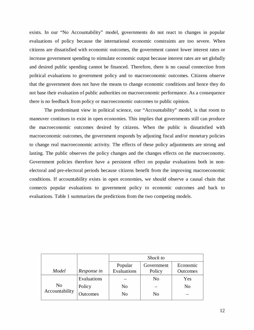
evaluations. Table 1 summarizes the predictions from the two competing models.
Shock to
Model
Response in
Popular Evaluations
Government Policy
Economic Outcomes
Evaluations – No Yes Policy No – No
No
Accountability Outcomes No No –
13
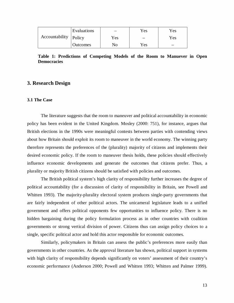
Evaluations – Yes Yes Policy Yes – Yes
Accountability
Outcomes No Yes –
Table 1: Predictions of Competing Models of the Room to Manuever in Open Democracies
3. Research Design
3.1 The Case
The literature suggests that the room to maneuver and political accountability in economic
policy has been evident in the United Kingdom. Mosley (2000: 751), for instance, argues that
British elections in the 1990s were meaningful contests between parties with contending views
about how Britain should exploit its room to maneuver in the world economy. The winning party
therefore represents the preferences of the (plurality) majority of citizens and implements their
desired economic policy. If the room to maneuver thesis holds, these policies should effectively
influence economic developments and generate the outcomes that citizens prefer. Thus, a
plurality or majority British citizens should be satisfied with policies and outcomes.
The British political system’s high clarity of responsibility further increases the degree of
political accountability (for a discussion of clarity of responsibility in Britain, see Powell and
Whitten 1993). The majority-plurality electoral system produces single-party governments that
are fairly independent of other political actors. The unicameral legislature leads to a unified
government and offers political opponents few opportunities to influence policy. There is no
hidden bargaining during the policy formulation process as in other countries with coalition
governments or strong vertical division of power. Citizens thus can assign policy choices to a
single, specific political actor and hold this actor responsible for economic outcomes.
Similarly, policymakers in Britain can assess the public’s preferences more easily than
governments in other countries. As the approval literature has shown, political support in systems
with high clarity of responsibility depends significantly on voters’ assessment of their country’s
economic performance (Anderson 2000; Powell and Whitten 1993; Whitten and Palmer 1999).
14
Among the major West European democracies, economic developments affect approval strongest
in Britain (Lewis-Beck 1988). British governments thus can infer from political approval and
evaluations of economic outcomes how citizens judge their performance. A decline in political
support and pessimistic economic expectations signal to the government that citizens are
dissatisfied with economic developments and prefer a policy change.
The United Kingdom therefore is a critical case and presents a natural experiment that
allows us to assess whether accountability exists in open economies. If political accountability in
fact existed in any economically open democracy, we should be able to observe it in the United
Kingdom. And if we do not find political accountability in Britain, it is unlikely that
accountability existed anywhere else.
To gauge the degree of accountability in Britain, we use multivariate time series analysis
of monthly economic and political data from April 1984 to September 2006. Measures of
economic openness show that by the late 1970s Britain was open to trade and capital flows. By
Quinn’s (2000) openness indicators, the British government had lifted nearly all restrictions to
capital mobility and trade by 1979. The current and capital account openness measures reach
their maximum values in 1979 and remain there until 1999 when the indicator ends. Quinn’s
measures also show that Britain was an open economy in relative terms. The indicator of overall
openness increases from 3.5 in 1950 to the maximum value 14 in 1979. Average overall openness
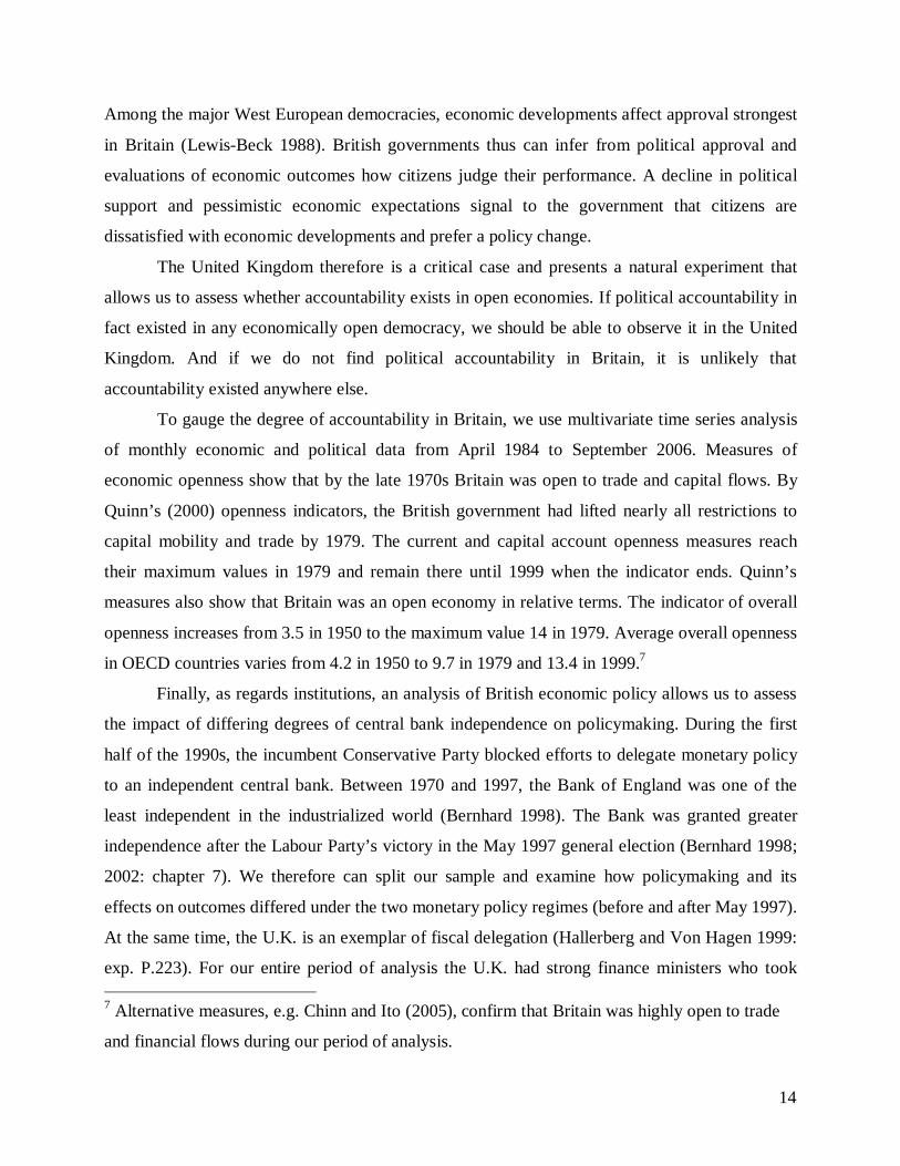
in OECD countries varies from 4.2 in 1950 to 9.7 in 1979 and 13.4 in 1999.7
Finally, as regards institutions, an analysis of British economic policy allows us to assess
the impact of differing degrees of central bank independence on policymaking. During the first
half of the 1990s, the incumbent Conservative Party blocked efforts to delegate monetary policy
to an independent central bank. Between 1970 and 1997, the Bank of England was one of the
least independent in the industrialized world (Bernhard 1998). The Bank was granted greater
independence after the Labour Party’s victory in the May 1997 general election (Bernhard 1998;
2002: chapter 7). We therefore can split our sample and examine how policymaking and its
effects on outcomes differed under the two monetary policy regimes (before and after May 1997).
At the same time, the U.K. is an exemplar of fiscal delegation (Hallerberg and Von Hagen 1999:
exp. P.223). For our entire period of analysis the U.K. had strong finance ministers who took 7 Alternative measures, e.g. Chinn and Ito (2005), confirm that Britain was highly open to trade
and financial flows during our period of analysis.
15
orders from prime ministers. The degree of transparency of fiscal policy making in the U.K. is
quite high.8
3.2 The Open Political Economy Framework
To gauge the degree of accountability in Britain, we combine current research from
political science and economics. Political scientists provide deep insights into the working of the
polity and how economic developments influence politics and policies. Economics helps us
understand how policy choices affect the macroeconomy and show which policies enhance
economic welfare. But, both disciplines ignore the feedback of policies, citizen’s preferences, and
macroeconomic activity. They therefore are incomplete for analyzing political accountability.9
Economic voting models are the natural starting point for a framework that allows for
endogeneity between the polity and the economy. These models show how voters continuously
evaluate the economic outcomes of government policies and then hold policymakers accountable
for them. If the economy is doing well (poorly), voters reward (punish) the government with
higher (lower) political support for the governing party. The key economic variables measuring
the state of the economy are unemployment, inflation, interest rates and the exchange rate (e.g.
Hibbs 1982; Sanders 1991).
Recent research has increasingly focused on the role of subjective rather than objective
evaluations, particularly for British political approval (Clarke et al. 2000; Clarke and Stewart
1995; Clarke et al. 1998; Sanders 1991; 2005). The literature suggests several indicators of
subjective evaluations reflecting citizen’s assessment of macroeconomic outcomes and
government policy. These indicators include personal financial expectations (Sanders 1991;
2005), personal and national retrospections (Kiewiet and Rivers 1985); and, forward-looking
assessments of economic forecasts rather than past economic outcomes (MacKuen et al. 1992).
Clarke and Stewart (1995) assess these competing indicators and find that personal expectations
subsume the personal retrospections, but not national expectations or national retrospections. 8 The U.K. ranks with France near the top of the Open Budget Index for the world’s
governments. See, The Economist, October 28, 2006, p. 114. 9 The only exception is Bernhard and Leblang (2006a). But their model does not include the
macroeconomy.
16
The recent literature’s shift toward subjective evaluations does not mean that objective
indicators are irrelevant. Political scientists are aware that “economic forces appear to influence
electors’ attitudes towards the economy in two different, if complementary ways” (Sanders 1991:
238). Objective variables influence personal and national economic expectations, which then are
transmitted to approval.
The new open macroeconomics literature generally refers to similar indicators reflecting
objective domestic economic developments as economic voting models. Empirical models of a
small open economy usually include measures of economic output, a price index, and monetary
policy variables, such as short-term interest rates. The international economy is represented by
foreign prices and foreign economic output. Exchange rates connect the domestic and the
international economy (Cushman and Zha 1997; Eichenbaum and Evans 1995; Kim 2001).
Depending on the specific research question, some studies add additional variables, such as the
trade balance (Betts and Devereux 2000) or exports and imports (Cushman and Zha 1997; Kim
2001). These variables essentially reflect the key components of the dynamic stochastic general
equilibrium models of small open economies (Betts and Devereux 2001; Galí and Monacelli
2005; Obstfeld and Rogoff 1995).
We use those variables that overlap in the political science and economics literature as a
basis of our open political economy model. These variables include domestic output and prices,
and the exchange rate. As in the open macroeconomics literature, we add an international
economy that is represented by foreign output and price levels. This setup is consistent with the
basic models that have been used in the open economy literature discussed above. The polity is
represented by the key components of economic voting models. Personal and sociotropic
economic expectations reflect how citizens subjectively assess the results from government
policies. Vote intentions and prime minister approval capture how citizens evaluate overall
government performance.
The policy sector that represents government policymaking includes domestic monetary
and fiscal policy. Since most of these empirical open economy models focus on transmission of
monetary policy, they generally neglect fiscal policy variables. The fiscal variable is important in
our context because the political science literature emphasizes the role of fiscal policy for room to
maneuver in open economies. To measure fiscal policy, we follow O'Mahony (2006), Clark and
Hallerberg (2000), and Hallerberg and von Hagen (1999) and use an indicator of the public

17
sector’s fiscal deficit. Such a deficit measure is appropriate for a test of the room to maneuver
thesis because it captures both government expenditure and income. The discrepancy between the
competing claims about room to maneuver in fiscal policy primarily arises from the studies’
focus on taxes or government spending. A complete analysis of room to maneuver has to take
into account both the income and the expenditure side.
Vote intentions (VIt) capture the percentage of voters who respond that they intend to vote
for the incumbent party. Prime minister approval (PMt) measures the percentage of respondents
who are satisfied with the performance of the prime minister. Subjective personal expectations
(PEt) are the difference between the proportion of people who expect that their personal financial
situation will improve during the next year and the proportion of people who think that their
situation will deteriorate. Subjective sociotropic expectations (SEt) capture the difference
between the proportion of people who expect that the national economic situation will improve
and the proportion of people who think that the situation will worsen. To capture electoral
dynamics, we use an electoral counter taking the value 1 in the month after each British general
election and increasing linearly to the next general election.
We use variables from the United States as a proxy for the world economy. The exchange
rate (XRt) thus is the monthly average of the $/£ nominal exchange rate; it corresponds to the
number of U.S. Dollars per British Pound. To measure economic output, we use the monthly
domestic and foreign Index of Industrial Production (IIPt and USIIPt). The domestic and foreign
price levels (CPIt and USCPIt) are from the British and U.S. Consumer Price Indices. Domestic
monetary and foreign monetary policies (IRt and USIRt) are the monthly average of short-term
interest rates in the two countries. British fiscal policy is the level of public sector debt (Gt). This
public sector debt index is based on the debt level reported by the government at the beginning of
the sample period. We then construct a monthly indicator of government debt using data on the
public sector net cash requirement. The net cash requirement indicates the amount that the British
government borrows from domestic and foreign investors to finance the difference between
public sector expenditures and receipts. For a detailed description of data sources and definitions,
see Appendix I.
3.3 Empirical Model and Structural Identification
18
To test the competing claims about the degree of political accountability in open
economies, we use Bayesian Structural Vector Autoregressive (B-SVAR) models. These are
appropriate for a problem like ours where model scale, endogeneity, persistence, and
specification uncertainty are present at the same time. B-SVAR models subsume more familiar
models like VARs, ECMs, and VECMs allowing for sounder statistical inferences. Details of the
B-SVAR model are described in Appendix II.
In a B-SVAR model our discussion of competing causal accounts of political
accountability is represented by different contemporaneous and lagged relationships among the
variables. The political and economic literatures imply a core set of relationships between the
variables within the polity and the economy. The two competing causal accounts (chains)—the
No Accountability and Accountability models—imply different contemporaneous relationships
across the polity and the economy: the immediate impact of political shocks on economic
variables and the immediate impact of economic shocks on political variables. Inferences about
the direction, magnitude, and duration of shocks in key variables can be made with the B-SVAR
models’ impulse responses. These impulse responses reveal the combined contemporaneous and
lagged relationships between the political and economic variables in the two models.
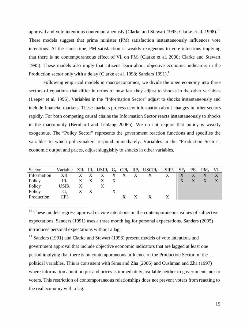
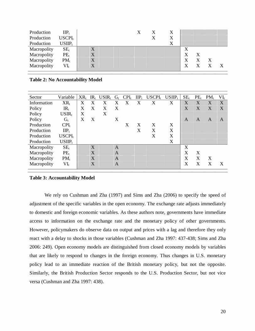
Tables 2 and 3 represent the contemporaneous relationships among the variables for the
competing No Accountability and the Accountability models. Each row in the tables corresponds
to an equation capturing the contemporaneous effect of the column variable on the row variable.
Empty cells are restrictions that mean that the column variable is assumed to have no
contemporaneous impact on the row equation. The X’s represent “free parameters” meaning that
the respective column variable can have an immediate impact on the row equation. The two
competing causal chains imply different X’s at the intersections of the policy and economy, the
grey-shaded fields in the upper right and lower left of the model specifications in Tables 2 and 3.
We rely on government approval research in Britain (Clarke et al. 2000; Clarke and
Stewart 1995) to identify the core political model in the lower right corner of each model in
Tables 2 and 3. The literature suggests that a lower-triangularized, contemporaneous order of SEt,
PEt, PMt and VIt is appropriate. The single-equation models of government approval used by
researchers imply that both sociotropic and personal subjective economic expectations affect
19
approval and vote intentions contemporaneously (Clarke and Stewart 1995; Clarke et al. 1998).10
These models suggest that prime minister (PM) satisfaction instantaneously influences vote
intentions. At the same time, PM satisfaction is weakly exogenous to vote intentions implying
that there is no contemporaneous effect of VIt on PMt (Clarke et al. 2000; Clarke and Stewart
1995). These models also imply that citizens learn about objective economic indicators in the
Production sector only with a delay (Clarke et al. 1998; Sanders 1991).11
Following empirical models in macroeconomics, we divide the open economy into three
sectors of equations that differ in terms of how fast they adjust to shocks in the other variables
(Leeper et al. 1996). Variables in the “Information Sector” adjust to shocks instantaneously and
include financial markets. These markets process new information about changes in other sectors
rapidly. For both competing causal chains the Information Sector reacts instantaneously to shocks
in the macropolity (Bernhard and Leblang 2006b). We do not require that policy is weakly
exogenous. The “Policy Sector” represents the government reaction functions and specifies the
variables to which policymakers respond immediately. Variables in the “Production Sector”,
economic output and prices, adjust sluggishly to shocks in other variables.
Sector Variable XRt IRt USIRt Gt CPIt IIPt USCPIt USIIPt SEt PEt PMt VIt Information XRt X X X X X X X X X X X X Policy IRt X X X X X X X X Policy USIRt X X Policy Gt X X X Production CPIt X X X X
10 These models regress approval or vote intentions on the contemporaneous values of subjective
expectations. Sanders (1991) uses a three month lag for personal expectations. Sanders (2005)
introduces personal expectations without a lag. 11 Sanders (1991) and Clarke and Stewart (1998) present models of vote intentions and
government approval that include objective economic indicators that are lagged at least one
period implying that there is no contemporaneous influence of the Production Sector on the
political variables. This is consistent with Sims and Zha (2006) and Cushman and Zha (1997)
where information about output and prices is immediately available neither to governments nor to
voters. This restriction of contemporaneous relationships does not prevent voters from reacting to
the real economy with a lag.
20
Production IIPt X X X Production USCPIt X X Production USIIPt X Macropolity SEt X X Macropolity PEt X X X Macropolity PMt X X X X Macropolity VIt X X X X X
Table 2: No Accountability Model
Sector Variable XRt IRt USIRt Gt CPIt IIPt USCPIt USIIPt SEt PEt PMt VIt Information XRt X X X X X X X X X X X X Policy IRt X X X X X X X X Policy USIRt X X Policy Gt X X X A A A A Production CPIt X X X X Production IIPt X X X Production USCPIt X X Production USIIPt X Macropolity SEt X A X Macropolity PEt X A X X Macropolity PMt X A X X X Macropolity VIt X A X X X X
Table 3: Accountability Model
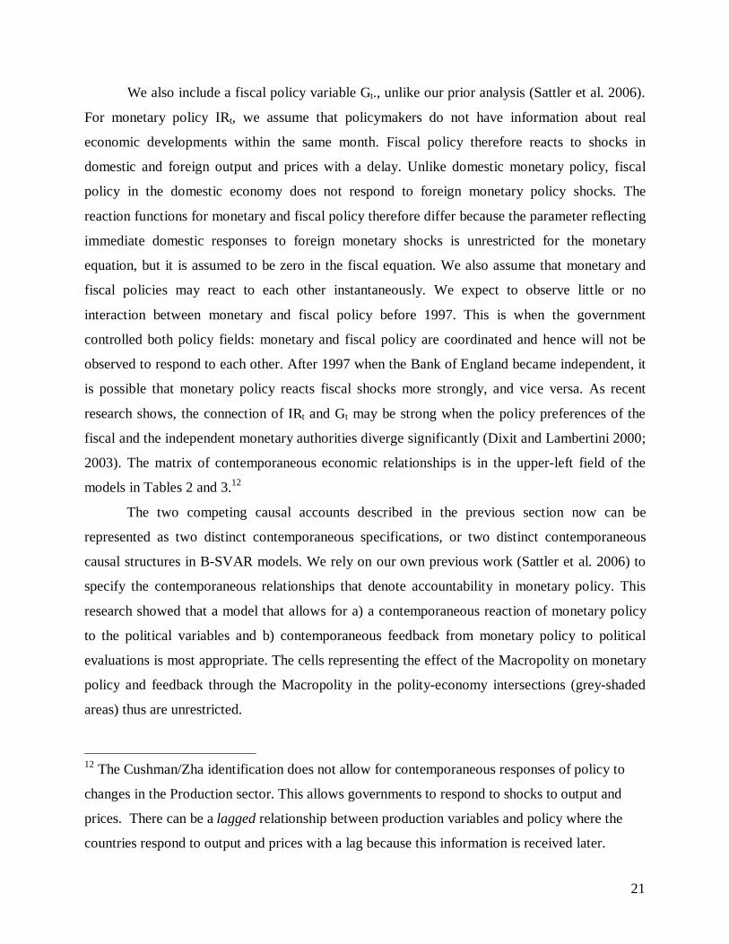
We rely on Cushman and Zha (1997) and Sims and Zha (2006) to specify the speed of
adjustment of the specific variables in the open economy. The exchange rate adjusts immediately
to domestic and foreign economic variables. As these authors note, governments have immediate
access to information on the exchange rate and the monetary policy of other governments.
However, policymakers do observe data on output and prices with a lag and therefore they only
react with a delay to shocks in those variables (Cushman and Zha 1997: 437-438; Sims and Zha
2006: 249). Open economy models are distinguished from closed economy models by variables
that are likely to respond to changes in the foreign economy. Thus changes in U.S. monetary
policy lead to an immediate reaction of the British monetary policy, but not the opposite.
Similarly, the British Production Sector responds to the U.S. Production Sector, but not vice
versa (Cushman and Zha 1997: 438).
21
We also include a fiscal policy variable Gt., unlike our prior analysis (Sattler et al. 2006).
For monetary policy IRt, we assume that policymakers do not have information about real
economic developments within the same month. Fiscal policy therefore reacts to shocks in
domestic and foreign output and prices with a delay. Unlike domestic monetary policy, fiscal
policy in the domestic economy does not respond to foreign monetary policy shocks. The
reaction functions for monetary and fiscal policy therefore differ because the parameter reflecting
immediate domestic responses to foreign monetary shocks is unrestricted for the monetary
equation, but it is assumed to be zero in the fiscal equation. We also assume that monetary and
fiscal policies may react to each other instantaneously. We expect to observe little or no
interaction between monetary and fiscal policy before 1997. This is when the government
controlled both policy fields: monetary and fiscal policy are coordinated and hence will not be
observed to respond to each other. After 1997 when the Bank of England became independent, it
is possible that monetary policy reacts fiscal shocks more strongly, and vice versa. As recent
research shows, the connection of IRt and Gt may be strong when the policy preferences of the
fiscal and the independent monetary authorities diverge significantly (Dixit and Lambertini 2000;
2003). The matrix of contemporaneous economic relationships is in the upper-left field of the
models in Tables 2 and 3.12
The two competing causal accounts described in the previous section now can be
represented as two distinct contemporaneous specifications, or two distinct contemporaneous
causal structures in B-SVAR models. We rely on our own previous work (Sattler et al. 2006) to
specify the contemporaneous relationships that denote accountability in monetary policy. This
research showed that a model that allows for a) a contemporaneous reaction of monetary policy
to the political variables and b) contemporaneous feedback from monetary policy to political
evaluations is most appropriate. The cells representing the effect of the Macropolity on monetary
policy and feedback through the Macropolity in the polity-economy intersections (grey-shaded
areas) thus are unrestricted.
12 The Cushman/Zha identification does not allow for contemporaneous responses of policy to
changes in the Production sector. This allows governments to respond to shocks to output and
prices. There can be a lagged relationship between production variables and policy where the
countries respond to output and prices with a lag because this information is received later.
22
The identification of the polity-economy intersections in the upper right and lower left
part of Table 2 represents the idea that no accountability in fiscal policy may exist in the open
economy. The distinguishing feature of this model is that the fiscal authority does not react
immediately to political shocks. The cells representing the influence of the Macropolity on fiscal
policy in the upper right corner are blank. Similarly, there is no impact of fiscal policy on the
polity, as the cells for the impact of fiscal policy on the Macropolity in the lower left corner of
Table 2 are empty. The model in Table 2 thus reflects the idea that accountability in monetary
policy may exist, but there is no accountability in fiscal policy.
The model in Table 3 modifies the identification restrictions in the polity-economy
intersections of this No Accountability model. This modification represents the “Accountability
Model” –the model that is necessary for Room to Maneuver – and allows the government to react
immediately to political shocks. The specification in the upper right corner of Table 3 shows the
modification of the matrix of contemporaneous relationships that leaves the fiscal responses to
political shocks unrestricted. The Accountability model also holds that the policy choices are
immediately evaluated, and feedback through the Macropolity exists. For such feedback to exist,
the contemporaneous relationships denoting the Macropolity’s reaction to fiscal shocks are
unrestricted in the Accountability model. The A’s in Table 3 represent these additional free
parameters that are necessary to allow for such contemporaneous government reaction and
feedback. The Accountability model thus has eight more free parameters than the No
Accountability model in Table 2.
3.4 Estimation
Because of the change that occurred in the monetary policy regime in the U.K. in 1997,
we estimated four B-SVAR models. The B-SVAR models use the No Accountability and
Accountability contemporaneous identification matrices specified earlier. Each of these structural
models is estimated using the monthly data series for the periods 1984:4-1997:4 and 1997:5-
2006:9. We will refer to the earlier period as the “Tory” period since the Thatcher and Major
governments were in power, and to the latter period as the “Labour” period since the Blair
governments have been in power. The interest rates, the exchange rate and the political variables
enter the model as proportions and the other economic variables enter the model in natural
23
logarithms. The four B-SVAR models all include six lags of the 12 endogenous variables in each
equation of the models. A single exogenous variable that is a local trend for the election periods
is included in each equation of the models as well. This variable counts the number of months
that each government is in power and resets to zero after each British election. It allows us to
gauge whether electorally induced monetary and fiscal “cycles” (Clark and Hallerberg 2000) are
evident in either period.
The prior distribution for the B-SVAR model is that proposed by Sims and Zha (1998); it
is consistent with the beliefs revealed by political scientists like Clarke, Stewart, and Sanders.13
The B-SVAR models with the Sims-Zha prior were estimated and their structural parameters
were sampled using a Gibbs sampler for B-SVAR proposed by Waggoner and Zha (2003a).
Details of the estimation can be found in Waggoner and Zha (2003a) , Brandt and Freeman
(2006b), and Sattler, Freeman and Brandt (2006).
All of the results reported here are based on a posterior sample of 20000 draws of the
model parameters after an initial burn-in of 5000 discarded draws. Analysis of the posterior
densities of the parameters (via traceplots, Geweke diagnostics, etc.) indicates that the parameter
draws have converged to stationary values. Earlier sensitivity analyses (for a similar model
without fiscal policy) showed that the results were generally insensitive to the specification of the
hyperparameters for the prior distribution for the B-SVAR model.
4. Results
4.1 Comparisons of Structural Specifications over the Tory and Labour Sub-Samples
To compare the competing Accountability and No Accountability structural models for
the Labour versus Tory time periods one can first look at Bayesian posterior odds measures.
13 The hyperparameter values for the prior are set at the standard reference values . The values are λ0=0.6, λ1=0.1, λ3=1, λ4=0.1, λ5=0.05, µ5=5, µ6=5. In an earlier paper, Sattler, Freeman and Brandt (2006) we conducted a sensitivity analysis using the reduced form representation of a similar model without the fiscal policy equation. This sensitivity analysis employed over 10,000 different sets of these hyperparameters and the prior employed here is among the best fitting from this sensitivity analysis (in terms of a log MDD criterion). Other hyperparameter values yield qualitatively similar inferences to those reported here. Therefore we believe that the results reported here are not sensitive to the prior we are using.
24
These measures compare the posterior odds that one model specification better explains the data
than another. These posterior odds measures are similar to a likelihood ratio statistic.
The posterior odds of the model specifications can be computed from the differences of
the log marginal data density (known also as marginal log likelihood) of the model. The log
marginal data density of the model is the log probability of the sample data conditional on the
model and its parameters and it measures the log posterior probability that the model explains the
data. The difference of the log marginal data densities for two models is known as the log Bayes
factor. This measures the weight of the evidence or posterior odds of one model versus another
(Kass and Raftery 1995).
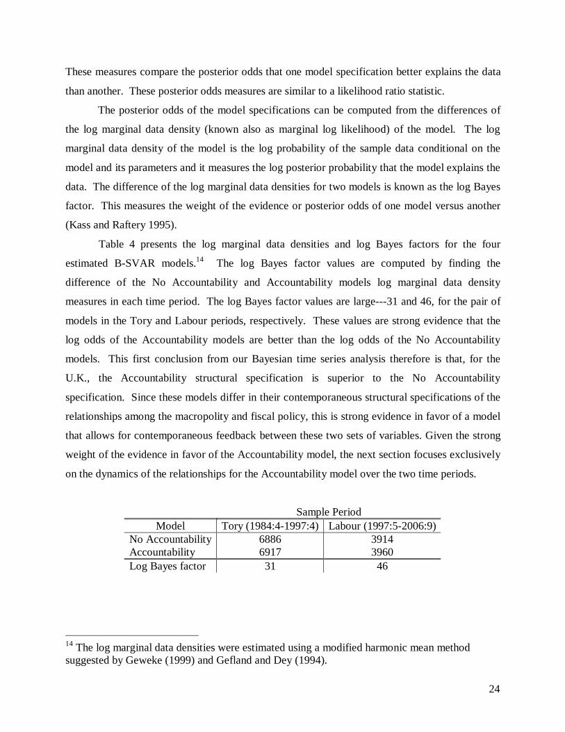
Table 4 presents the log marginal data densities and log Bayes factors for the four
estimated B-SVAR models.14 The log Bayes factor values are computed by finding the
difference of the No Accountability and Accountability models log marginal data density
measures in each time period. The log Bayes factor values are large---31 and 46, for the pair of
models in the Tory and Labour periods, respectively. These values are strong evidence that the
log odds of the Accountability models are better than the log odds of the No Accountability
models. This first conclusion from our Bayesian time series analysis therefore is that, for the
U.K., the Accountability structural specification is superior to the No Accountability
specification. Since these models differ in their contemporaneous structural specifications of the
relationships among the macropolity and fiscal policy, this is strong evidence in favor of a model
that allows for contemporaneous feedback between these two sets of variables. Given the strong
weight of the evidence in favor of the Accountability model, the next section focuses exclusively
on the dynamics of the relationships for the Accountability model over the two time periods.
Sample Period Model Tory (1984:4-1997:4) Labour (1997:5-2006:9)
No Accountability 6886 3914 Accountability 6917 3960 Log Bayes factor 31 46
14 The log marginal data densities were estimated using a modified harmonic mean method suggested by Geweke (1999) and Gefland and Dey (1994).
25
Table 4: Log marginal data densities for the Four B-SVAR Models for the Tory and
Labour Periods and Log Bayes Factors Comparing the Odds of the Accountability and No
Accountability Models Over Each Period.
4.2 Dynamic Inferences
The dynamics of the Accountability models for the Tory versus Labour government
periods can be evaluated using impulse response functions (IRFs). IRFs allow us to trace out the
response of a standardized shock in each variable in each equation over time. These impulse
response functions are computed from the reduced form representation of the two accountability
models, one each for the Tory and Labour periods. The IRFs presented here are computed from
the fitted B-SVAR models and summarized with likelihood-based error bands (Brandt and
Freeman 2006b; Sims and Zha 1999). The responses are median estimates over 24 months with
68% likelihood-based error bands. 15
The analysis of accountability concerns a subset of the 12 x 12 = 144 impulse responses
for each B-SVAR model. These subsets are 1) monetary policy reactions to political evaluations
(the macropolity variables), 2) fiscal policy reactions to political evaluations, 3) public responses
to monetary policy, 4) the public’s responses to fiscal policy, 5) reactions of the real economy to
fiscal and monetary policy shocks, and 6) reactions of the public to shocks to the real economy.
For each of these six sets of IRFs, the Tory and Labour period responses from the
Accountability model will be presented together. The Tory period (1984:4-1997:4)
Accountability model responses are represented with solid lines with 68% error bands and the
Labour period (1997:5-2006:9) Accountability model responses are represented with dashed lines
with 68% error bands. Because these are IRFs for a structural model, the shocks to each equation
15 All of the responses are based on the 20000 draws from the structural parameters of the model. These are mapped into the reduced form parameters to compute the IRFs. The likelihood-based error bands are from the eigendecomposition of each IRF shock-response. The eigen-decompositions first component of each IRF shock-response combination is used to compute the width of the error bands. These first components of each response explain over 90% of the variation in the responses over 24 months. These error bands thus differ from Sattler et al. (2006) which used empirical percentiles for the error bands. Further, note that the split and shorter samples used here mean that the empirical percentile error bands would be much larger in this paper, compared to Sattler et al. (2006). This means that we need to better account for the serial correlation of the responses, which the eigendecomposition method does.
26
do not necessarily always have the same sign (i.e., are not positive). In B-SVAR models, the
likelihood is invariant to the signs of the structural shocks, so it can be the case that a positive
structural shock to one equation implies a negative structural shock to another equation (e.g.,
shocks to negatively correlated series will have opposite signs). For the two B-SVAR
Accountability models the pattern of the signs of the shocks across the equations is not the same
across the two models. While one might normalize the shocks to have similar signs, this ignores
the cross equation sign patterns that are important for understanding monetary-fiscal policy
interactions and accountability across the Tory and Labour regimes. Thus the discussion below
takes care to explain the direction of the shocks and pattern of responses for each equation.16
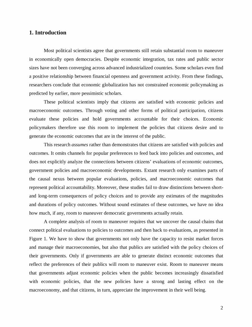
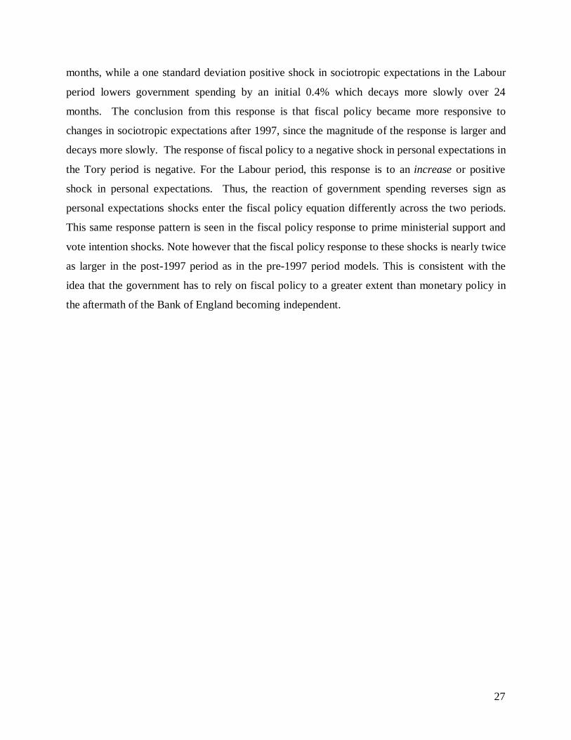
Figure 1 shows the response of UK interest rates to shocks in the macropolity variables.
Since the own shock to interest rates is negative in both the Tory and Labor periods of the
accountability models, these responses are the reactions to one standard deviation declines in
sociotropic and personal expectations, prime ministerial support, and vote intentions. In both the
1984-1997 and 1997-2006 periods, a decline in sociotriopic expectations leads to an increase in
interest rates, while the reverse happens for personal expectations. A negative shock to or decline
in prime ministerial support lowers interest rates in the Tory period but increases interest rates in
the Labour period. Note that the impact in the latter period when the Bank of England is
independent is about a third of the reaction seen in the earlier period. Finally, a decrease in vote
intentions leads to an increase in interest rates in the Tory period, but no real change in interest
rates in the later Labour period. These latter interest rate responses support the idea that as the
central bank became more independent after 1997, the impacts of public approval of the
government and vote intentions on interest rates diminished.
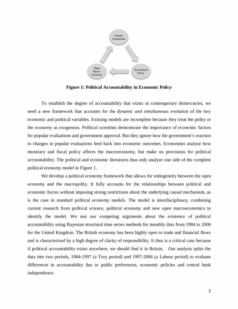
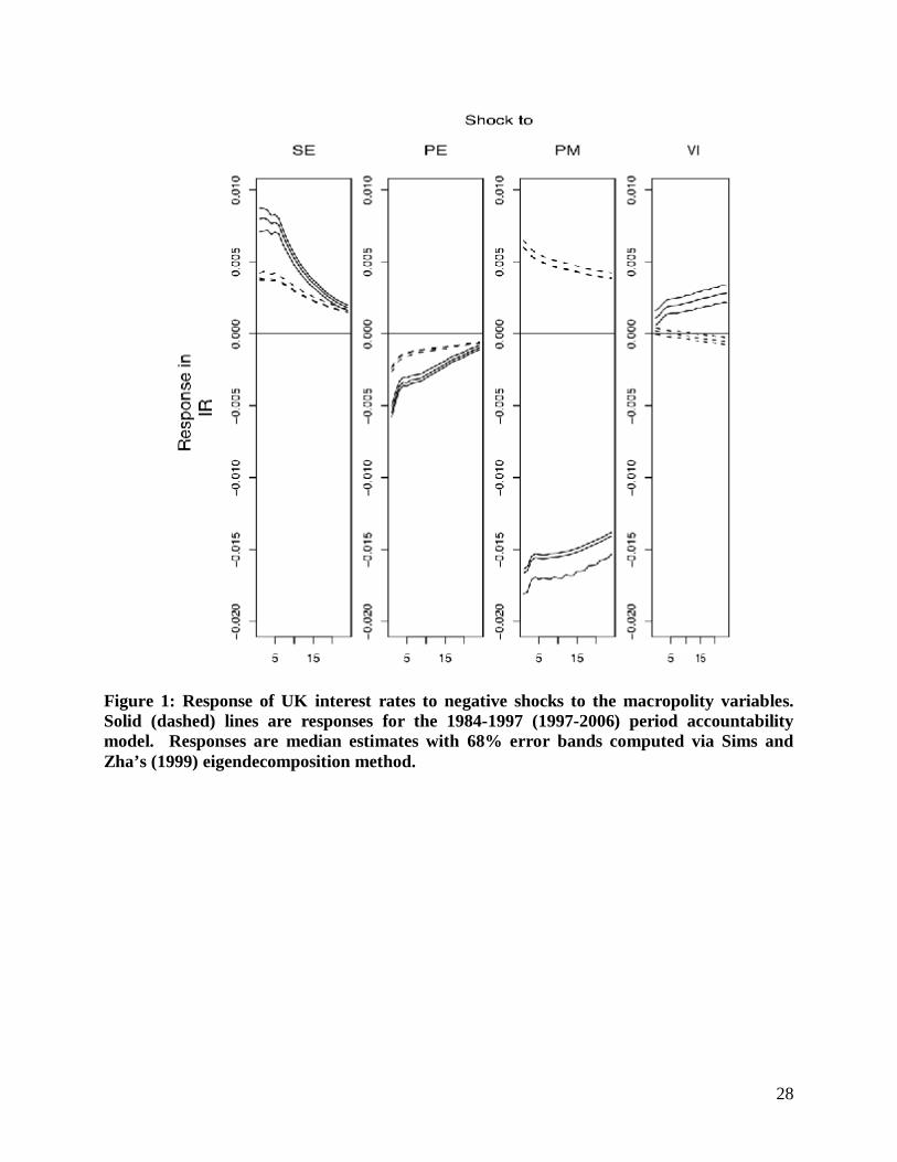
Figure 2 shows the response of our fiscal policy index to shocks in the four macropolity
variables. In the Tory (Labour) period model these shocks enter the equation negatively
(positively). So the impact of a standard deviation negative shock in sociotropic expectations in
the Tory period is an increase in government spending by an initial 0.15% which decays over 24
16 The signs of the diagonal A(0) matrices are normalized to have the same signs in the draws from the Gibbs sampler. However, the pattern of signs used differs across the A(0) matrices for the Accountability model for the Tory and Labour periods. For more detail on the sign normalization used in Gibbs sampling B-SVAR models see Waggoner and Zha (2003b). The pattern of the signs for the 12 elements of the Accountability model diagonal of the A(0) matrices in the Tory (Labour) period model is +,-,-,-,-,-,-,-,-,-,-,- (+,-,-,+,-,-,-,-,-,-,+,+). So there is no simple sign renormalization to make the models for the two periods easily comparable.
27
months, while a one standard deviation positive shock in sociotropic expectations in the Labour
period lowers government spending by an initial 0.4% which decays more slowly over 24
months. The conclusion from this response is that fiscal policy became more responsive to
changes in sociotropic expectations after 1997, since the magnitude of the response is larger and
decays more slowly. The response of fiscal policy to a negative shock in personal expectations in
the Tory period is negative. For the Labour period, this response is to an increase or positive
shock in personal expectations. Thus, the reaction of government spending reverses sign as
personal expectations shocks enter the fiscal policy equation differently across the two periods.
This same response pattern is seen in the fiscal policy response to prime ministerial support and
vote intention shocks. Note however that the fiscal policy response to these shocks is nearly twice
as larger in the post-1997 period as in the pre-1997 period models. This is consistent with the
idea that the government has to rely on fiscal policy to a greater extent than monetary policy in
the aftermath of the Bank of England becoming independent.
28
Figure 1: Response of UK interest rates to negative shocks to the macropolity variables. Solid (dashed) lines are responses for the 1984-1997 (1997-2006) period accountability model. Responses are median estimates with 68% error bands computed via Sims and Zha’s (1999) eigendecomposition method.
29
Figure 2: Response of UK public sector debt index (fiscal policy) to shocks to the macropolity variables. Solid (dashed) lines are responses for the 1984-1997 (1997-2006) period accountability model. One standard deviation structural shocks enter the Tory (Labour) period equation with negatively (positively). Responses are median estimates with 68% error bands computed via Sims and Zha’s (1999) eigendecomposition method.
30
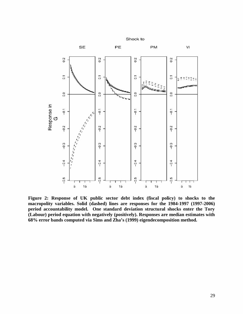
Figure 3 shows the responses of the macropolity variables to policy innovations in interest
rates and fiscal policy. Interest rate shocks have no or small effects on the sociotropic or personal
expectations equations in either period. The policy shocks enter the prime ministerial support
and vote intention equations as negative (positive) one standard deviation changes in the Tory
(Labour) period. So surprise decreases in interest rates lead to higher prime ministerial support in
the Tory period, but surprise increases in interest rates generate the same response in the Labour
period. The Labour period prime ministerial support response is about twice as large as that seen
in the earlier period. Vote intentions respond in a similar fashion: negative shocks in interest
rates increase vote intentions for the government party in the Tory period. Positive shocks in
interest rates decrease vote intentions in the Labour period. So the general relationship is the
same: higher interest rates lower vote intentions for the government party, but this effect is
weaker in the latter period of the data, perhaps because citizens know that elected officials enjoy
less control over monetary policy. Our results also indicate that conservative governments receive
more support when there are lower interest rates while liberal governments receive less support
when there are higher interest rates.
The responses of the macropolity to fiscal policy shocks are shown in the second column
of Figure 3. Fiscal policy shocks in both periods are negative in the sociotropic and personal
expectations equations. Thus, fiscal policy contractions initially lower (increase) sociotropic
expectations in the Labour (Tory) periods. These effects are both initially negative, but the
Labour period sociotropic expectations response to fiscal contractions becomes positive after 10
months. The negative fiscal policy shocks to the personal expectations equation produce
different initial and delayed responses. As fiscal policy contracts in the Tory period, personal
expectations decline and then become positive after about 5 months. During the Labour period,
the initial response is positive and increases slowly over 24 months. In the main, fiscal
contraction leads eventually to higher personal expectations in the Tory period than in the Labour
period with the differences emerging after 15 months.
31
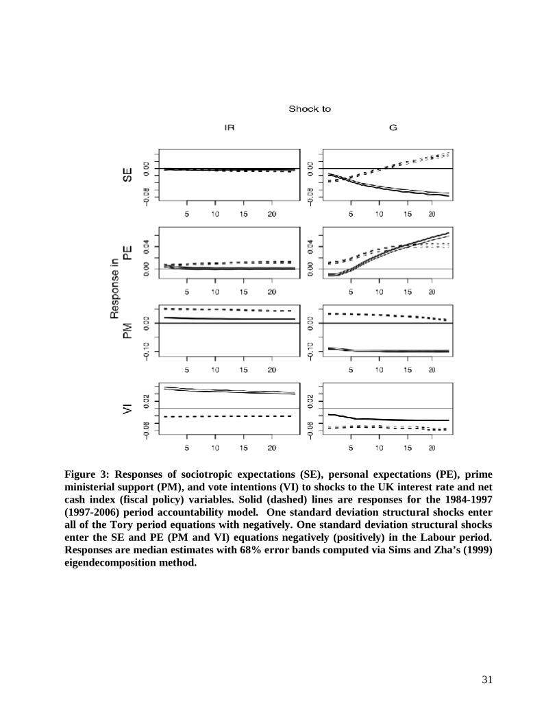
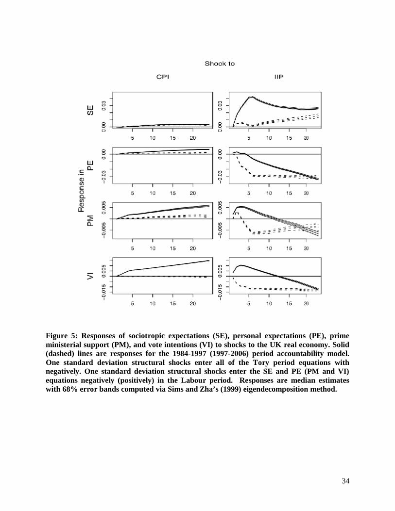
Figure 3: Responses of sociotropic expectations (SE), personal expectations (PE), prime ministerial support (PM), and vote intentions (VI) to shocks to the UK interest rate and net cash index (fiscal policy) variables. Solid (dashed) lines are responses for the 1984-1997 (1997-2006) period accountability model. One standard deviation structural shocks enter all of the Tory period equations with negatively. One standard deviation structural shocks enter the SE and PE (PM and VI) equations negatively (positively) in the Labour period. Responses are median estimates with 68% error bands computed via Sims and Zha’s (1999) eigendecomposition method.
32
The responses of prime ministerial support and vote intentions to fiscal policy changes
also are shown in Figure 3. Shocks to these two equations enter as contractions (expansions) in
fiscal policy for the Tory (Labour) periods. So a surprise contraction in fiscal policy generates a
decline in prime ministerial support and vote intentions in the Tory period. In the Labour period,
an unexpected fiscal expansion increases prime ministerial support, but lowers vote intentions.
This supports the argument that the impacts of fiscal policy are inverted in the Labour versus
Tory periods, since contractions (expansions) is fiscal policy generate different signed vote
intention responses.
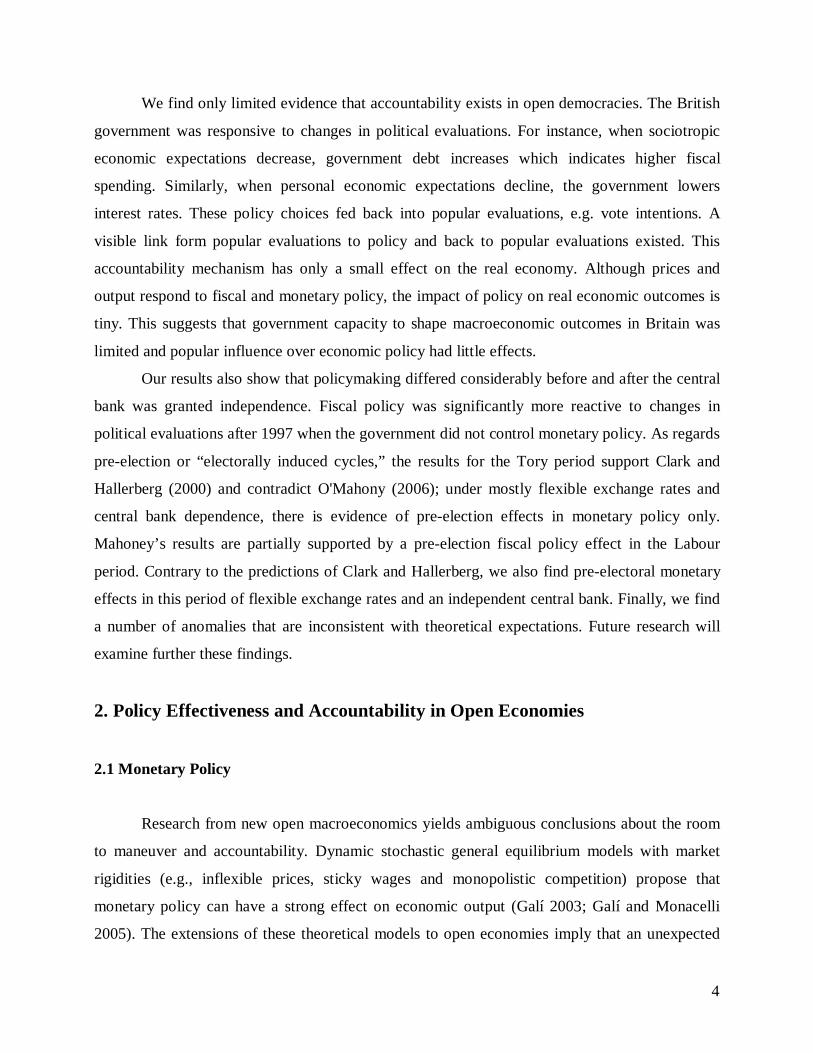
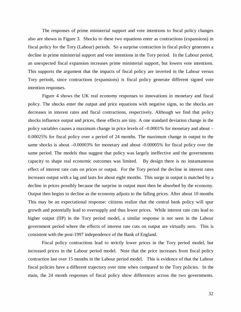
Figure 4 shows the UK real economy responses to innovations in monetary and fiscal
policy. The shocks enter the output and price equations with negative signs, so the shocks are
decreases in interest rates and fiscal contractions, respectively. Although we find that policy
shocks influence output and prices, these effects are tiny. A one standard deviation change in the
policy variables causes a maximum change in price levels of –0.0001% for monetary and about –
0.00025% for fiscal policy over a period of 24 months. The maximum change in output to the
same shocks is about –0.00003% for monetary and about -0.00005% for fiscal policy over the
same period. The models thus suggest that policy was largely ineffective and the governments
capacity to shape real economic outcomes was limited. By design there is no instantaneous
effect of interest rate cuts on prices or output. For the Tory period the decline in interest rates
increases output with a lag and lasts for about eight months. This surge in output is matched by a
decline in prices possibly because the surprise in output must then be absorbed by the economy.
Output then begins to decline as the economy adjusts to the falling prices. After about 10 months
This may be an expectational response: citizens realize that the central bank policy will spur
growth and potentially lead to oversupply and thus lower prices. While interest rate cuts lead to
higher output (IIP) in the Tory period model, a similar response is not seen in the Labour
government period where the effects of interest rate cuts on output are virtually zero. This is
consistent with the post-1997 independence of the Bank of England.
Fiscal policy contractions lead to strictly lower prices in the Tory period model, but
increased prices in the Labour period model. Note that the price increases from fiscal policy
contraction last over 15 months in the Labour period model. This is evidence of that the Labour
fiscal policies have a different trajectory over time when compared to the Tory policies. In the
main, the 24 month responses of fiscal policy show differences across the two governments.
33
Finally, fiscal policy contractions lead to lower production in the Tory period. However, for the
Labour period model, industrial production increases for about 20 months and then declines.
Comparing the responses in Figure 4 the shifts in central bank policy and fiscal policy are clear:
the room to maneuver shifts from monetary policy under the Tory governments to fiscal policy
under the later Labour governments. These results on fiscal policy shocks are clearly anomalous.
Future work will look at possible additions to the model that address these results. Examples
include allowing IIP to be contemporaneously related to G.
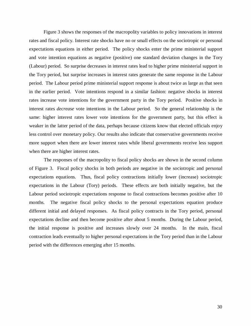
Figure 4: Response of UK real economy to shocks to the interest rate and fiscal policy variables. Solid (dashed) lines are responses for the 1984-1997 (1997-2006) period accountability model. Structural shocks enter the CPI and IIP equations with negative signs. Responses are median estimates with 68% error bands computed via Sims and Zha’s (1999) eigendecomposition method.
34
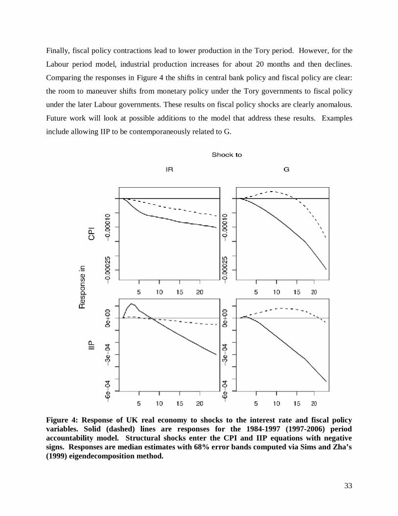
Figure 5: Responses of sociotropic expectations (SE), personal expectations (PE), prime ministerial support (PM), and vote intentions (VI) to shocks to the UK real economy. Solid (dashed) lines are responses for the 1984-1997 (1997-2006) period accountability model. One standard deviation structural shocks enter all of the Tory period equations with negatively. One standard deviation structural shocks enter the SE and PE (PM and VI) equations negatively (positively) in the Labour period. Responses are median estimates with 68% error bands computed via Sims and Zha’s (1999) eigendecomposition method.
35
Figure 5 shows the final part of the accountability chain: the impacts of the real economy
on the macropolity variables. The price (CPI) and production (IIP) shocks enter the sociotropic
and personal expectations equations as deflationary impacts. Price deflation thus has very weak
positive impacts on expectations over 24 months. The impacts of negative shocks in production
are more complex. Declines in production generate higher sociotropic expectations. This Tory
period response is nearly four times larger than the Labour period response. This makes sense if
one considers that higher sociotropic expectations mean that people feel that others are doing
better—or that as the economy contracts that people think they are worse off than others.
Personal expectations decline quickly in response to the surprise drop in production. During the
Tory period, the decline in personal expectations initially is small but after about 5 months drops
rapidly for the next 24 months. During the Labour period model, the drop in personal
expectations from a negative shock in IIP is nearly immediate and reaches its “bottom” after
about 6 months. Thus, the reaction time of personal expectations differs greatly across the two
governments and reflects how much more people see there personal circumstances tied to the
economy in the recent Labour governments.
The prime ministerial support and vote intention equations have shocks that enter the
Accountability model with different signs across the two periods. Negative (positive) shocks
enter these equations in the Tory (Labour) period of the model. Thus, as prices drop in the Tory
period, prime ministerial support and vote intentions rise, presumably as (Labour) voters are
willing to cross-over and reward the government. In the Labour government periods, similar
shocks generate tiny responses that are hardly different from zero. Thus, one sees that during the
Tory period there was significant sensitivity to prices for both measures of government support.
The reactions of prime ministerial support and vote intentions to production shocks are
much stronger. As production declines in the Tory period model, prime ministerial support and
vote intentions are initially positive. This decays over about a year, eventually leading a slip in
government support that is equal to the initial increase. Thus, short term declines in production
under the Tory period model are met with a rise in government support, but this slips away as the
real economy continues to falter. Thus, public evaluations of the government (versus personal
and sociotropic expectations) respond to the real economy with a longer lag. The responses of the
government support variables to the positive shocks or production expansions in the Labour
period model have a different pattern. Initially, prime ministerial support rises, but it quickly
36
drops. The same negative pattern is seen in vote intentions. Industrial production increases
actually hurt the Labour government support over a two-year period. This response, like those
seen for the real economy is also anomalous because we would expect different signs. One might
conjecture that the Labour period governments concern with globalization and reduced control
over monetary policy may make the public concerned about other economic and policy issues.
The coefficients on our electoral dummy variables allow us to assess competing results about the
existence of pre-electoral or “electorally induced” policy cycles. The densities for these
coefficients presented in Figure 6. According to Clarke and Hallerberg (2000), because for most
of the Tory period, the U.K. had a dependent central bank, capital mobility, and a flexible
exchange, we should find pre-electoral monetary effects only.17 The results for the IR and G
equations are consistent with this prediction; the coefficient in the interest rate equation indicates
that in the run up to elections Tories lowered interest rates while they made no changes in fiscal
policy. This is inconsistent with O'Mahony’s (2006) new results which predicts that because of
Britain’s trade openness and flexible exchange rates, pre-electoral fiscal expansions should occur.
In contrast the results for the Labour period are more consistent with O'Mahoney’s argument;
they contradict Clark and Hallerberg. The coefficient on the electoral dummy in the G equation in
the period 1997-2006 is nonzero but, surprisingly, negative indicating a fiscal contraction in the
run up to elections. There also is evidence of pre-electoral monetary effects—an anomalous rise
in interest rates—in this period. Because the Bank of England is independent in this period of
capital mobility and flexible exchange rate Clark and Hallerberg predict neither kind of effect.
17 According the Reinhard and Rogoff (2004) index, the UK had flexible exchange rates between 1984 and September 1990; relatively fixed exchanges between September 1990 and the end of 1992; and then flexible exchange rates until 2001.
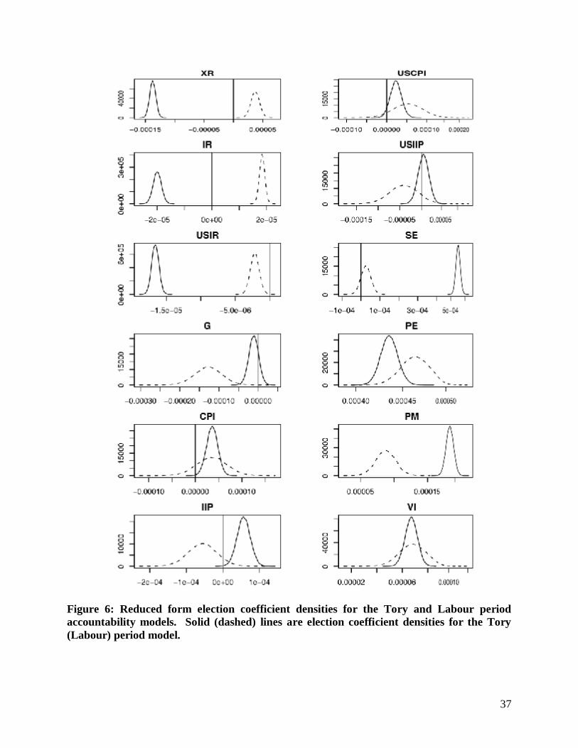
37
Figure 6: Reduced form election coefficient densities for the Tory and Labour period accountability models. Solid (dashed) lines are election coefficient densities for the Tory (Labour) period model.
38
5. Conclusion
Our results are only partially consistent with the room to maneuver thesis. We find that
the British government was responsive to changes in political evaluations of policies and
outcomes. The public thus can induce policy changes and exerts some influence over
policymaking. Voters then react to policy changes through changes in political support for the
government. But there is only little evidence that the government can effectively influence real
economy outcomes. The effects of monetary and fiscal policy on economic output and prices are
negligible. Therefore, the accountability mechanism largely works outside the real economy. In
terms of the full relationship between the economy and the policy described in Figure 1, there is
only little transmission of policy through the economy. The links from policy to the economy are
weak. The reason for this main finding seems to be that the public simply does not appreciate the
limited impact that economic policy has on the real economy, regardless of central bank
independence.
Future research should address a number of anomalies that are inconsistent with
theoretical expectations. Refinements of the structural identification schemes can help to assess
the dynamic relationship of political and economic processes further. We will also continue to
evaluate the impact of different priors on the estimation results. Finally, alternative measures of
fiscal policy may help to better understand the use of fiscal policy instruments and economic
policymaking in general.
39
Appendix I: Data Description and Sources
Political Variables
The political series are from different polling institutes in Britain. Vote intentions (VIt),
prime minister approval (PMt) and subjective sociotropic expectations (SEt) are from MORI.
Vote intentions capture the percentage of voters who respond that they intend to vote for the
incumbent party.18 Prime minister approval measures the percentage of respondents who are
satisfied with the performance of the Prime Minister.19 Subjective sociotropic expectations
capture the difference between the proportion of people who expect that the national economic
situation will improve and the proportion of people who think that the situation will worsen.20
Subjective personal expectations (PEt) are the difference between the proportion of people
who expect that their personal financial situation will improve during the next year and the
proportion of people who think that their situation will deteriorate. The data are from the Gallup
Organization (King and Wybrow 2001) until December 2002 and from YouGov for January 2003
onwards.21 The series has to be spliced together from different sources because Gallup stopped
collect these data in 2003, but YouGov only started its survey in 2002. Generally, the YouGov
series of personal expectations is 11 percentage points lower than the equivalent Gallup series.
An adjustment factor of +11 is added to the YouGov series to make the data comparable (Sanders
2005: Appendix). We are grateful to Harold Clarke for providing these data.
Economic Variables
The exchange rate XRt is from the database of the Bank of England.It is the monthly
average of the $/£ nominal exchange rate. The British Index of Industrial Production (IIPt) is
from the Office of National Statistics time series database. U.S. Index of Industrial Production
(USIIPt) is provided by the Federal Reserve Bank. Consumer Prices (CPIt) are from the IMF
18 http://www.ipsos-mori.com/polls/trends/voting-all-trends.shtml 19 http://www.ipsos-mori.com/polls/trends/satisfac.shtml 20 http://www.ipsos-mori.com/polls/trends/economy.shtml 21 http://www.yougov.com
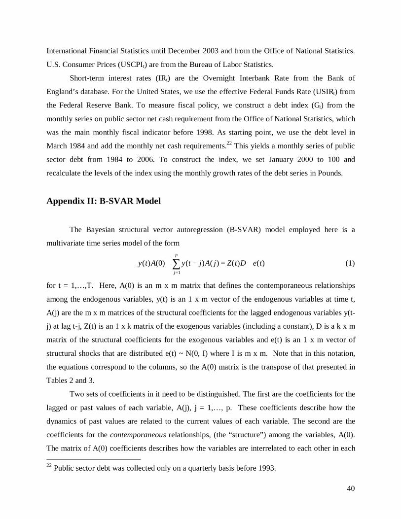
40
International Financial Statistics until December 2003 and from the Office of National Statistics.
U.S. Consumer Prices (USCPIt) are from the Bureau of Labor Statistics.
Short-term interest rates (IRt) are the Overnight Interbank Rate from the Bank of
England’s database. For the United States, we use the effective Federal Funds Rate (USIRt) from
the Federal Reserve Bank. To measure fiscal policy, we construct a debt index (Gt) from the
monthly series on public sector net cash requirement from the Office of National Statistics, which
was the main monthly fiscal indicator before 1998. As starting point, we use the debt level in
March 1984 and add the monthly net cash requirements.22 This yields a monthly series of public
sector debt from 1984 to 2006. To construct the index, we set January 2000 to 100 and
recalculate the levels of the index using the monthly growth rates of the debt series in Pounds.
Appendix II: B-SVAR Model
The Bayesian structural vector autoregression (B-SVAR) model employed here is a
multivariate time series model of the form
y(t)A(0) + y(t − j)A( j) = Z(t)D + e(t)j=1
p
∑ (1)
for t = 1,…,T. Here, A(0) is an m x m matrix that defines the contemporaneous relationships
among the endogenous variables, y(t) is an 1 x m vector of the endogenous variables at time t,
A(j) are the m x m matrices of the structural coefficients for the lagged endogenous variables y(t-
j) at lag t-j, Z(t) is an 1 x k matrix of the exogenous variables (including a constant), D is a k x m
matrix of the structural coefficients for the exogenous variables and e(t) is an 1 x m vector of
structural shocks that are distributed e(t) ~ N(0, I) where I is m x m. Note that in this notation,
the equations correspond to the columns, so the A(0) matrix is the transpose of that presented in
Tables 2 and 3.
Two sets of coefficients in it need to be distinguished. The first are the coefficients for the
lagged or past values of each variable, A(j), j = 1,…, p. These coefficients describe how the
dynamics of past values are related to the current values of each variable. The second are the
coefficients for the contemporaneous relationships, (the “structure”) among the variables, A(0).
The matrix of A(0) coefficients describes how the variables are interrelated to each other in each 22 Public sector debt was collected only on a quarterly basis before 1993.
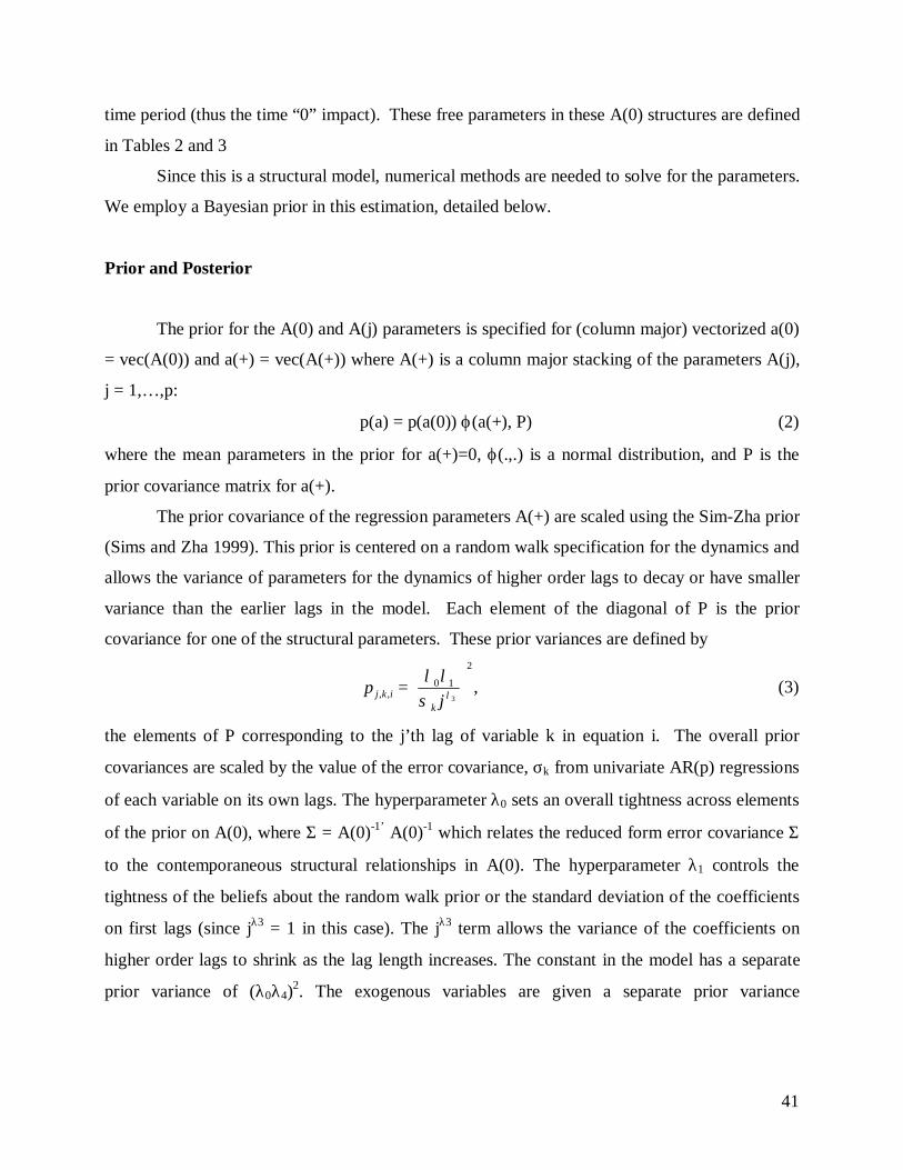
41
time period (thus the time “0” impact). These free parameters in these A(0) structures are defined
in Tables 2 and 3
Since this is a structural model, numerical methods are needed to solve for the parameters.
We employ a Bayesian prior in this estimation, detailed below.
Prior and Posterior
The prior for the A(0) and A(j) parameters is specified for (column major) vectorized a(0)
= vec(A(0)) and a(+) = vec(A(+)) where A(+) is a column major stacking of the parameters A(j),
j = 1,…,p:
p(a) = p(a(0)) ϕ(a(+), P) (2)
where the mean parameters in the prior for a(+)=0, ϕ(.,.) is a normal distribution, and P is the
prior covariance matrix for a(+).
The prior covariance of the regression parameters A(+) are scaled using the Sim-Zha prior
(Sims and Zha 1999). This prior is centered on a random walk specification for the dynamics and
allows the variance of parameters for the dynamics of higher order lags to decay or have smaller
variance than the earlier lags in the model. Each element of the diagonal of P is the prior
covariance for one of the structural parameters. These prior variances are defined by
p j,k,i =λ0λ1
σ k j λ3
2
, (3)
the elements of P corresponding to the j’th lag of variable k in equation i. The overall prior
covariances are scaled by the value of the error covariance, σk from univariate AR(p) regressions
of each variable on its own lags. The hyperparameter λ0 sets an overall tightness across elements
of the prior on A(0), where Σ = A(0)-1’ A(0)-1 which relates the reduced form error covariance Σ
to the contemporaneous structural relationships in A(0). The hyperparameter λ1 controls the
tightness of the beliefs about the random walk prior or the standard deviation of the coefficients
on first lags (since jλ3 = 1 in this case). The jλ3 term allows the variance of the coefficients on
higher order lags to shrink as the lag length increases. The constant in the model has a separate
prior variance of (λ0λ4)2. The exogenous variables are given a separate prior variance
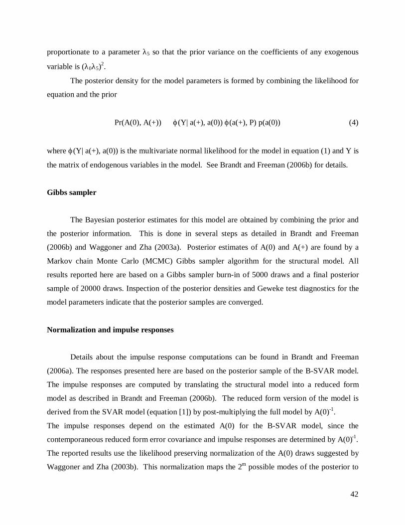
42
proportionate to a parameter λ5 so that the prior variance on the coefficients of any exogenous
variable is (λ0λ5)2.
The posterior density for the model parameters is formed by combining the likelihood for
equation and the prior
Pr(A(0), A(+)) ∝ ϕ(Y| a(+), a(0)) ϕ(a(+), P) p(a(0)) (4)
where ϕ(Y| a(+), a(0)) is the multivariate normal likelihood for the model in equation (1) and Y is
the matrix of endogenous variables in the model. See Brandt and Freeman (2006b) for details.
Gibbs sampler
The Bayesian posterior estimates for this model are obtained by combining the prior and
the posterior information. This is done in several steps as detailed in Brandt and Freeman
(2006b) and Waggoner and Zha (2003a). Posterior estimates of A(0) and A(+) are found by a
Markov chain Monte Carlo (MCMC) Gibbs sampler algorithm for the structural model. All
results reported here are based on a Gibbs sampler burn-in of 5000 draws and a final posterior
sample of 20000 draws. Inspection of the posterior densities and Geweke test diagnostics for the
model parameters indicate that the posterior samples are converged.
Normalization and impulse responses
Details about the impulse response computations can be found in Brandt and Freeman
(2006a). The responses presented here are based on the posterior sample of the B-SVAR model.
The impulse responses are computed by translating the structural model into a reduced form
model as described in Brandt and Freeman (2006b). The reduced form version of the model is
derived from the SVAR model (equation [1]) by post-multiplying the full model by A(0)-1.
The impulse responses depend on the estimated A(0) for the B-SVAR model, since the
contemporaneous reduced form error covariance and impulse responses are determined by A(0)-1.
The reported results use the likelihood preserving normalization of the A(0) draws suggested by
Waggoner and Zha (2003b). This normalization maps the 2m possible modes of the posterior to

43
an unique A(0). This normalized set of A(0) draws does not imply the innovations are all
positive shocks in the structural model since positive shocks to one equation might imply
negative shocks to another equation.
44
References
Anderson, Christopher J. (2000). "Economic Voting and Political Context: A
Comparative Perspective." Electoral Studies 19: 151-170.
Bearce, David (forthcoming). Monetary Divergence: Domestic Policy Autonomy in the
Post-Bretton Woods Era. Ann Arbor, University of Michigan Press.
Bernauer, Thomas and Christoph Achini (2000). "From 'Real' to 'Virtual' States?:
Integration of the World Economy and its Effects on Government Activity." European Journal of
International Relations 6: 223-276.
Bernhard, William (1998). "A Political Explanation of Variations in Central Bank
Independence." American Political Science Review 92: 311-328.
Bernhard, William (2002). Banking on Reform: Political Parties and Central Bank
Independence in the Industrial Democracies. Ann Arbor, The University of Michigan Press.
Bernhard, William and David Leblang (2006a). "Polls and Pounds: Exchange Rate
Volatility and Domestic Political Competition in Britain." Quarterly Journal of Political Science
1: 25-47.
Bernhard, William T. and David Leblang (2006b). Democratic Processes and Financial
Markets: Pricing Politics. New York, Cambridge University Press.
Betts, Caroline and Michael B. Devereux (2000). "Exchange Rate Dynamics in a Model
of Pricing-to-Market." Journal of International Economics 50: 215-244.
Betts, Caroline and Michael B. Devereux (2001). "The International Effects of Monetary
and Fiscal Policy in a Two-Country Model." In: M. Obstfeld and G. Calvo, eds. Esseys in Honor
of Robert A. Mundell. Cambridge, MIT Press: 9-52.
Brandt, Patrick and John R. Freeman (2006a). "Advances in Bayesian Time Series
Modeling and the Study of Politics: Theory Testing, Forecasting, and Policy Analysis." Political
Analysis 14: 1-36.
Brandt, Patrick and John R. Freeman (2006b). "Modeling Macro Political Dynamics."
Unpublished Manuscript. University of Minnesota, Twin Cities.
http://www.polisci.umn.edu/faculty/freeman/brandt-freeman-2006.pdf.
45
Bretschger, Lucas and Frank Hettich (2002). "Globalisation, Capital Mobility and Tax
Competition: Theory and Evidence for OECD Countries." European Journal of Political
Economy 18: 695-716.
Bretschger, Lucas and Frank Hettich (2005). "Globalisation and International Tax
Competition: Empirical Evidence Based on Effective Tax Rates." Journal of Economic
Integration 20: 530-542.
Clarida, Richard and Jordi Galí (1994). "Sources of Real Exchange Rate Fluctuations:
How Important are Nominal Shocks?" NBER Working Paper Series 4658.
Clark, William R. and Mark Hallerberg (2000). "Mobile Capital, Domestic Institutions,
and Electorally Induced Monetary and Fiscal Policy." American Political Science Review 94:
323-346.
Clarke, Harold, Karl Ho and Marianne C. Stewart (2000). "Major's lesser (not Minor)
Effects: Prime Ministerial Approval and Governing Party Support in Britain Since 1979."
Electoral Studies 19: 255-273.
Clarke, Harold and Marianne C. Stewart (1995). "Economic Evaluations, Prime
Ministerial Approval and Governing Party Support: Rival Models Reconsidered." British Journal
of Political Science 25: 145-170.
Clarke, Harold, Marianne C. Stewart and Paul F. Whiteley (1998). "New Models for New
Labour: The Political Economy of Labour Party Support, January 1992-April 1997." American
Political Science Review 92: 559-575.
Cushman, David O. and Tao Zha (1997). "Identifying Monetary Policy in a Small Open
Economy under Flexible Exchange Rates." Journal of Monetary Economics 39: 433-448.
Dixit, Avinash and Luisa Lambertini (2000). "Fiscal Discretion Destroys Monetary
Commitment." Manuscript. Princeton University.
Dixit, Avinash and Luisa Lambertini (2003). "Interactions of Commitment and Discretion
in Monetary and Fiscal Policies." American Economic Review 93: 1522-1542.
Eichenbaum, Martin and Charles L. Evans (1995). "Some Emprical Evidence on the
Shocks to Monetary Policy on Exchange Rates." The Quarterly Journal of Economics 110: 975-
1009.
Frieden, Jeffry A. (1991). "Invested Interests: The Politics of National Economic Policies
in a World of Global Finance." International Organization 45: 425-451.
46
Galí, Jordi (2003). "New Perspectives on Monetary Policy, Inflation, and the Business
Cycle." In: M. Dewatripont, L. P. Hansen and S. J. Turnovsky, eds. Advances in Economics and
Econometrics: Theory and Applications, Eighth World Congress. Cambridge, Cambridge
University Press. 3: 151-197.
Galí, Jordi and Tommaso Monacelli (2005). "Monetary Policy and Exchange Rate
Volatility in a Small Open Economy." Review of Economic Studies 72: 707-734.
Garrett, Geoffrey (1998a). "Global Markets and National Politics: Collision Course or
Virtuous Circle?" International Organization 52: 787-824.
Garrett, Geoffrey (1998b). Partisan Politics in the Gobal Economy. New York,
Cambridge University Press.
Garrett, Geoffrey and Deborah Mitchell (2001). "Globalization, Government Spending
and Taxation in the OECD." European Journal of Political Research 39: 145-177.
Gelfand, Alan E. and Dipak Dey, K. (1994). "Bayesian Model Choice: Asymptotics and
Exact Calculations." Journal of the Royal Statistical Society. Series B (Methodological) 56: 501-
514.
Genschel, Philipp (2002). "Globalization, Tax Competition, and the Welfare State."
Politics and Society 30: 245-275.
Geweke, John (1999). "Using Simulation Methods for Bayesian Econometric Models:
Inference, Development, and Communication." Econometric Reviews 18: 1-73.
Hallerberg, Mark and Jürgen Von Hagen (1999). "Electoral Institutions, Cabinet
Negotiations and Budget Deficits within the European Union." In: J. Poterba and J. Von Hagen,
eds. Fiscal Institutions and Fiscal Performance. Chicago, University of Chicago Press: 209-232.
Hibbs, Douglas (1982). "Economic Outcomes and Political Support for British
Governments Among Occupational Classes: A Dynamic Analysis." American Political Science
Review 76: 259-279.
Kass, Robert E. and Adrian E. Raftery (1995). "Bayes Factors." Journal of the American
Statistical Assocation 90: 773-795.
Kiewiet, D. Roderick and Douglas Rivers (1985). "A Retrospective on Retrospective
Voting." In: H. Eulau and M. S. Lewis-Beck, eds. Economic Conditions and Electoral Outcomes.
New York, Agathon Press.
47
Kim, Soyoung (2001). "International Transmission of U.S. Monetary Policy Shocks:
Evidence from VAR's." Journal of Monetary Economics 48: 339-372.
Leeper, Eric M., Christopher A. Sims and Tao A. Zha (1996). "What Does Monetary
Policy Do?" Brookings Papers on Economic Activity 1996: 1-63.
Leeper, Jonathan and Gabriel Sterne (2002). "Parliamentary Scrunity of Central Banks in
the United Kingdom and Overseas." Bank of England Quarterly Bulletin 42: 274-285.
Lewis-Beck, Michael S. (1988). Economics and Elections: The Major Western
Democracies. Ann Arbor, The University of Michigan Press.
MacKuen, Michael B., Robert S. Erikson and James A. Stimson (1992). "Peasants or
Bankers? The American Electorate and the U.S. Economy." American Political Science Review
86: 597-611.
Mosley, Layna (2000). "Room to Move: International Financial Markets and National
Welfare States." International Organization 54: 737-773.
O'Mahony, Angela (2006). "Engeneering Good Times: Fiscal Manipulation in a Global
Economy." Paper Presented at the Inaugural Meeting of the International Political Economy
Society, November 17-18, Princeton University.
Obstfeld, Maurice and Kenneth Rogoff (1995). "Exchange Rate Dynamics Redux."
Journal of Political Economy 103: 624-660.
Powell, G. Bingham and Garry D. Whitten (1993). "A Cross-National Analysis of
Economic Voting: Taking Account of the Political Context." American Journal of Political
Science 37: 391-414.
Quinn, Dennis (1997). "The Correlates of Change in International Financial Regulation."
American Journal of Political Science 91: 531-551.
Quinn, Dennis P. (2000). "Democracy and International Financial Liberalization."
Unpublished Manuscript. Washington D.C. http://faculty.msb.edu/quinnd/papers/demfin.pdf.
Reinhart, Carmen M. and Kenneth Rogoff (2004). "The Modern History of Exchange
Rate Arrangements: A Reinterpretation." Quarterly Journal of Economics 119: 1-48.
Rodrik, Dani (1998). "Why Do More Open Economies Have Bigger Governments?"
Journal of Political Economy 106: 997-1032.
Sanders, David (1991). "Government Popularity and the Next General Election." Political
Quarterly 62: 235-261.
48
Sanders, David (2005). "The Political Economy of UK Party Support, 1997-2004:
Forcasts for the 2005 General Election." Journal of Elections, Public Opinion, and Parties 15:
47-71.
Sattler, Thomas, John R. Freeman and Patrick T. Brandt (2006). "Political Accountability
and the Room to Maneuver: A Search for a Causal Chain." Manuscript. Minneapolis, MN.
http://www.polisci.umn.edu/faculty/freeman/wp.php.
Sims, Christopher A. and Tao A. Zha (1998). "Bayesian Methods for Dynamic
Multivariate Models." International Economic Review 39: 949-968.
Sims, Christopher A. and Tao A. Zha (1999). "Error Bands for Impulse Responses."
Econometrica 67: 1113-1156.
Sims, Christopher A. and Tao A. Zha (2006). "Does Monetary Policy Generate
Recessions?" Macroeconomic Dynamics 10: 231-272.
Swank, Duane and Sven Steinmo (2002). "The New Political Economy of Taxation in
Advanced Capitalist Democracies." American Journal of Political Science 46: 642-655.
Tanzi, Victor (1996). "Globalization, Tax Competition, and the Future of Tax Systems."
IMF Working Paper WP/96/141.
Waggoner, Daniel F. and Tao A. Zha (2003a). "A Gibbs Sampler for Structural Vector
Autoregressions." Journal of Dynamics and Control 28: 349-366.
Waggoner, Daniel F. and Tao A. Zha (2003b). "Likelihood Preserving Normalization in
Multiple Equation Models." Journal of Econometrics 114: 329-347.
Whitten, Guy D. and Harvey D. Palmer (1999). "Cross-National Analyses of Economic
Voting." 18: 49-67.