Economic Roundup Issue 3, 2010 - Estimating the structural ...archive.treasury.gov.au/documents/1881/PDF/04_Structural_Budget... · benefited from comments and ... structural and

51

Estimating the structural budget balance of the Australian Government Tony McDonald, Yong Hong Yan, Blake Ford and David Stephan1

This paper develops estimates of the structural budget balance of the Australian Government. It describes the methodology and assumptions used in developing these estimates, includes sensitivity analysis, and explains why these estimates differ from those produced by the IMF and OECD.

1 The authors are from Macroeconomic Group, the Australian Treasury. This article has benefited from comments and suggestions provided by David Gruen, Damien White, John Clark, Steve Morling, Adam McKissack, Phil Garton, Jin Liu, and Shane Brittle. The views in this article are those of the authors and not necessarily those of the Australian Treasury.

Estimating the structural budget balance of the Australian Government

52

Introduction

The Australian Government’s medium-term fiscal strategy includes a commitment to achieve budget surpluses on average over the medium term. Further, the Charter of Budget Honesty Act 1998 requires the Government to publish a fiscal strategy statement that, among other things, explains key fiscal measures against which fiscal policy will be set and assessed.

In this context, it would clearly be desirable to have a definitive measure of the Australian Government’s budget adjusting for the economic cycle, separating movements in the budget position between cyclical and structural components. The importance of such measures includes that the appropriate fiscal policy response to structural and cyclical shifts in the budget position is likely to be different (For a fuller discussion on this point, see Chalk, 2002; Mercereau and Razhkov, 2006; Price, Joumard, Andre and Minegishi, 2008.)

Even if a definitive measure could be found, it would only cover one aspect of an assessment of fiscal sustainability. The state of the Government’s balance sheet, including the level of contingent liabilities and other risks, and the outlook for long term economic growth are also important elements of fiscal sustainability.

In practice, there are a range of approaches to obtain these estimates, the results of which can vary markedly. Typically, such measures involve considerable complexity and uncertainty (Ford, 2005). There is therefore a need to exercise caution in the interpretation of structural budget balance measures. In particular, excessive reliance on point estimates should be avoided.

The 2009-10 Budget included estimates of the structural budget balance of the Australian Government in the context of a broader analysis of fiscal sustainability. This paper updates these estimates and describes the methodology and assumptions used in their development. The main way our estimates differ from most other approaches is that they adjust for movements in Australia’s terms of trade and for cyclical variations in capital gains taxes.

The paper starts by outlining the major steps involved in structural budget balance measures and explaining the methodology adopted for each of these steps for our structural budget balance measure. It then examines the key drivers of movements in the measure over time, and analyses the sensitivity of the measure to key assumptions, such as the terms of trade and the level of productivity. The paper concludes by comparing the estimates with those produced by the IMF and OECD, and explaining the key factors driving the differences between them.


53

Steps in calculating structural budget balance measures

While a variety of approaches have been developed to decompose government revenue and expenditure into cyclical and structural components, the most common broad approach is that outlined by Giorno, Richardson, Roseveare and van den Noord (1995) and van den Noord (2000). Under this approach, the structural component is determined residually, as the budget balance adjusted for the estimated impact of cyclical factors. The components of the budget position are assumed to be additive: that is, by assumption movements in the budget balance are either cyclical or structural. That is:

Actual Budget Balance = Structural Component + Cyclical Component

The impact of cyclical factors on the budget is determined by comparing an estimated ‘structural’ or potential level of nominal GDP with its actual or projected level, and then multiplying this difference by estimated elasticities for the revenue and expenditure components of the budget affected by cyclical factors.2 That is:

Cyclical Component = [Nominal GDP — Structural GDP] x Relevant Elasticities

Within this common broad approach, a number of assumptions are required to generate a structural budget balance estimate. Box 1 outlines the methods used by the IMF and OECD to calculate structural budget balances. As there are a number of different approaches to the steps involved in the calculation of structural budget balances, estimates can vary significantly, have a wide margin of error and require careful interpretation (Ford, 2005). Just as measures of the structural or potential level of output are subject to significant revision, so too are structural budget balance estimates that rely on those measures (Gruen, Robinson and Stone, 2005; Price, Joumard, Andre and Minegishi, 2008).

It is therefore important for the proper interpretation of estimates of the structural budget balance that their methodology, assumptions and limitations are set out clearly. The following sections set out the key steps involved in the calculation of our estimates of the structural budget balance.

2 The forecasts and projections for GDP in this paper are as set out in the 2010 Pre-election Economic and Fiscal Outlook.


54

Box 1: IMF and OECD structural budget balance methodologies

The IMF and OECD regularly publish updated estimates of structural budget balances for a range of countries. Both the IMF (De Masi, 1997; Hagemann, 1999; Fedelino, Ivanova and Horton, 2009) and OECD (Giorno, Richardson, Roseveare and van den Noord, 1995; Sukyer, 1999; Girouard and Andre, 2005) have published papers explaining their methodology in detail. This Box summarises these methodologies.

Both the IMF and OECD start by estimating an economy’s potential output. For most countries this is done using a two-factor constant returns-to-scale Cobb-Douglas production function. Potential output is calculated as the level of output consistent with an economy’s stock of capital and ‘non-accelerating inflation rate of unemployment’ (NAIRU).

The next step is estimating the cyclical component of revenues and expenditures and subtracting this from the totals. Both the IMF and OECD measures identify the cyclical component of budget aggregates by estimating the responsiveness of actual revenue and expenditure to deviations from the economy’s potential level of output.

Both methods estimate the cyclical component of revenue using elasticities for major tax revenue heads drawn from the OECD’s Economic Outlook Database. These elasticities are calculated for four tax categories: personal, corporate, indirect and social security contributions. While both measures draw on the same primary source for these elasticities, the OECD individually adjusts revenue for each major tax item whereas the IMF uses an aggregate elasticity that reflects the weighted share of each tax category in total revenue (Ford 2005).

Both measures assume that unemployment benefits are the only cyclical component of expenditures. The IMF and OECD both assume a proportionate change in unemployment benefits when the unemployment rate deviates from the NAIRU. However, while the IMF assumes a unitary elasticity of unemployment benefits with respect to the gap between the unemployment rate and the NAIRU, the OECD econometrically estimates this relationship for each country.

Finally, Structural Budget Balance estimates are then calculated by subtracting the cyclically adjusted expenditure from cyclically adjusted revenue.


55

Calculation of structural level of GDP

The structural level of GDP in the model is derived using a deterministic trend, similar to that adopted by the European Commission (Roger and Ongena, 1995). This approach involves making explicit assumptions about the key components of the structural level of GDP.

The structural level of nominal GDP is derived by combining a structural level of real GDP with a structural GDP deflator. The assumptions underpinning these estimates are outlined in the following sections.

Calculation of structural level of GDP: real GDP

The structural level of real GDP is derived from assumptions of the key underlying components. Real GDP can be decomposed into labour productivity (real GDP per hour worked) and total hours worked in the economy. In turn, the total hours worked in the economy is the product of the working age population, the participation rate, the employment rate and average hours worked per employee (Treasury, 2000; Henry, 2001). That is:

Real GDP = Labour Productivity x Total Hours Worked

Labour Productivity = Real GDP per Hour Worked

Total Hours Worked = Working Age Population x Participation Rate x (1 - Unemployment Rate) x Average Hours Worked.

The approach adopted in relation to each of these components of real GDP is outlined below.

Labour productivity

The medium term projections assume that labour productivity will grow at its 30 year average of 1.6 per cent per annum.

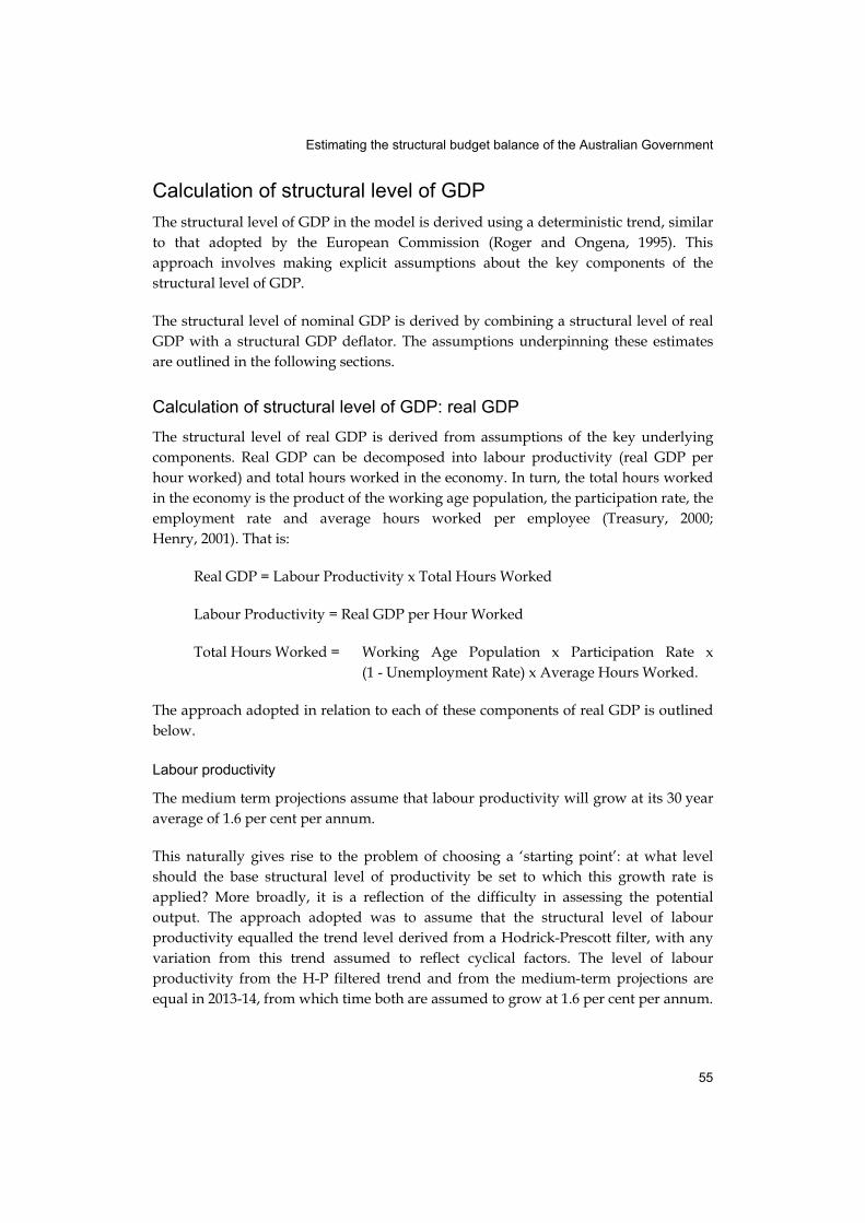
This naturally gives rise to the problem of choosing a ‘starting point’: at what level should the base structural level of productivity be set to which this growth rate is applied? More broadly, it is a reflection of the difficulty in assessing the potential output. The approach adopted was to assume that the structural level of labour productivity equalled the trend level derived from a Hodrick-Prescott filter, with any variation from this trend assumed to reflect cyclical factors. The level of labour productivity from the H-P filtered trend and from the medium-term projections are equal in 2013-14, from which time both are assumed to grow at 1.6 per cent per annum.


56

The resultant structural productivity level compared with the actual or projected level of labour productivity is presented at Chart 1 below.

Chart 1: Structural productivity assumption

75

80

85

90

75

80

85

90

2001-02 2003-04 2005-06 2007-08 2009-10 2011-12 2013-14

Structural labour productivity Actual/Projected labour productivity

Index (2020-21= 100) Index (2020-21= 100)

Source: ABS cat. no. 5204.0 and Treasury.

Working Age Population

The calculation of the structural level of real GDP assumes that the Working Age Population (defined as the population aged 15 and over) is not affected by cyclical factors. Therefore, the structural level of the Working Age Population is assumed to be equal to its actual level in history and the projections outlined in the medium-term fiscal projections.

While there is likely to be some degree of cyclicality in the net overseas migration component of Working Age Population, this is hard to separate from (larger) structural changes over time. That said, further work into this issue could prove to be a useful extension of this model.

Participation rate

The economic projections underpinning the medium-term fiscal estimates take into account the impact of demographic trends on the participation rate, particularly the impact of the ‘baby boom’ generation shifting out of the ‘peak’ participation age groups over time. These trends are structural in nature, and are therefore allowed for in the structural budget balance model.


57

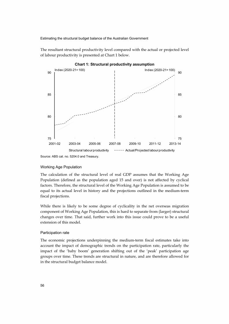
When the unemployment rate is rising, some workers are assumed to leave the labour force, and vice versa. The medium-term model also takes into account these encouraged/discouraged worker effects on the participation rate. The structural participation rate is the actual/projected participation rate less the encouraged worker effect.

Chart 2: Structural participation rate assumption

62.0

62.5

63.0

63.5

64.0

64.5

65.0

65.5

66.0

62.0

62.5

63.0

63.5

64.0

64.5

65.0

65.5

66.0

2001-02 2003-04 2005-06 2007-08 2009-10 2011-12 2013-14

Participation rateParticipation rate

Structural participation rate Actual/Projected participation rate


Unemployment rate

The structural real GDP assumes a constant unemployment rate of 5 per cent over the period. This is consistent with the assumed level of the non-accelerating inflation rate of unemployment (NAIRU) in the economic projections underpinning the medium-term fiscal projections.

Hours worked per employee

The average level of hours worked per employee has changed over time, reflecting a combination of structural and cyclical factors.

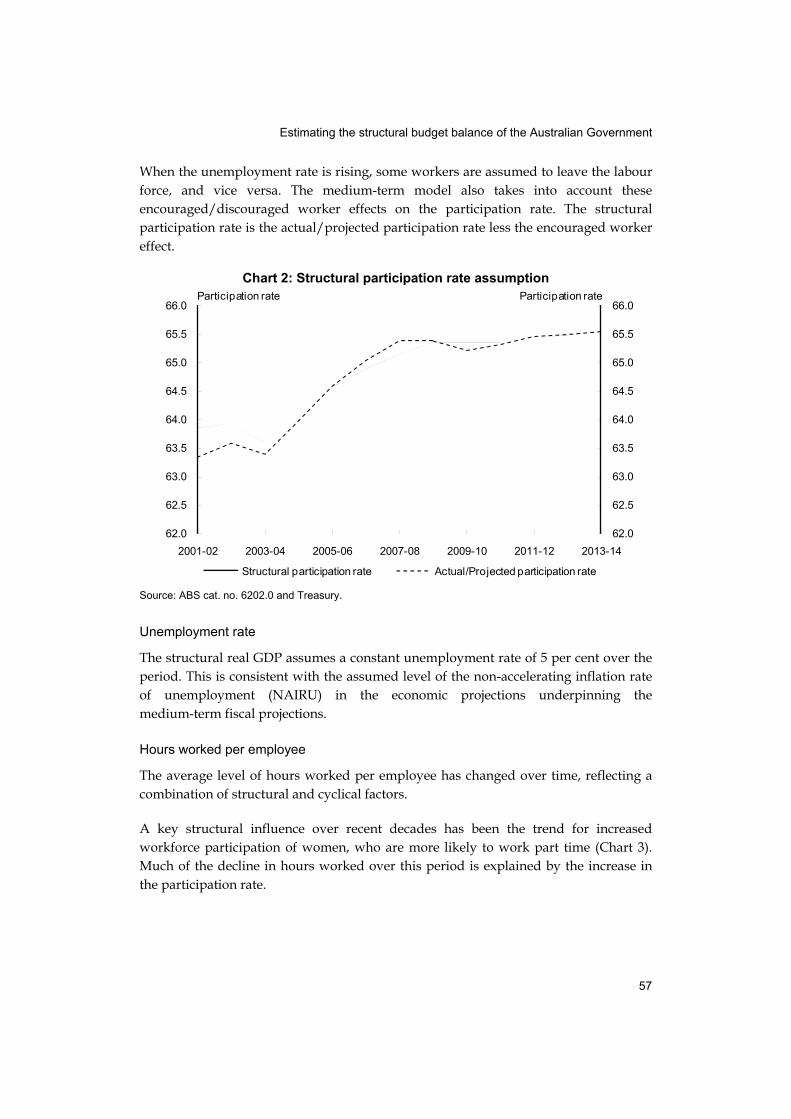
A key structural influence over recent decades has been the trend for increased workforce participation of women, who are more likely to work part time (Chart 3). Much of the decline in hours worked over this period is explained by the increase in the participation rate.


58

Chart 3: Hours worked per employee

62.5

63.0

63.5

64.0

64.5

65.0

65.5

66.032.0

32.5

33.0

33.5

34.0

34.5

35.0

1989-90 1993-94 1997-98 2001-02 2005-06 2009-10 2013-14

Average hours worked per employee (LHS) Participation rate (RHS)

Hours worked per week Participation rate (inverted)

Source: ABS cat. no. 6203.0 and 6202.0.

It is likely that there is also a cyclical element in the average hours worked per employee. In particular, average hours worked per employee is likely to fall in a recession, as employers faced with falling demand seek to retain staff by reducing the hours of their full time employees.

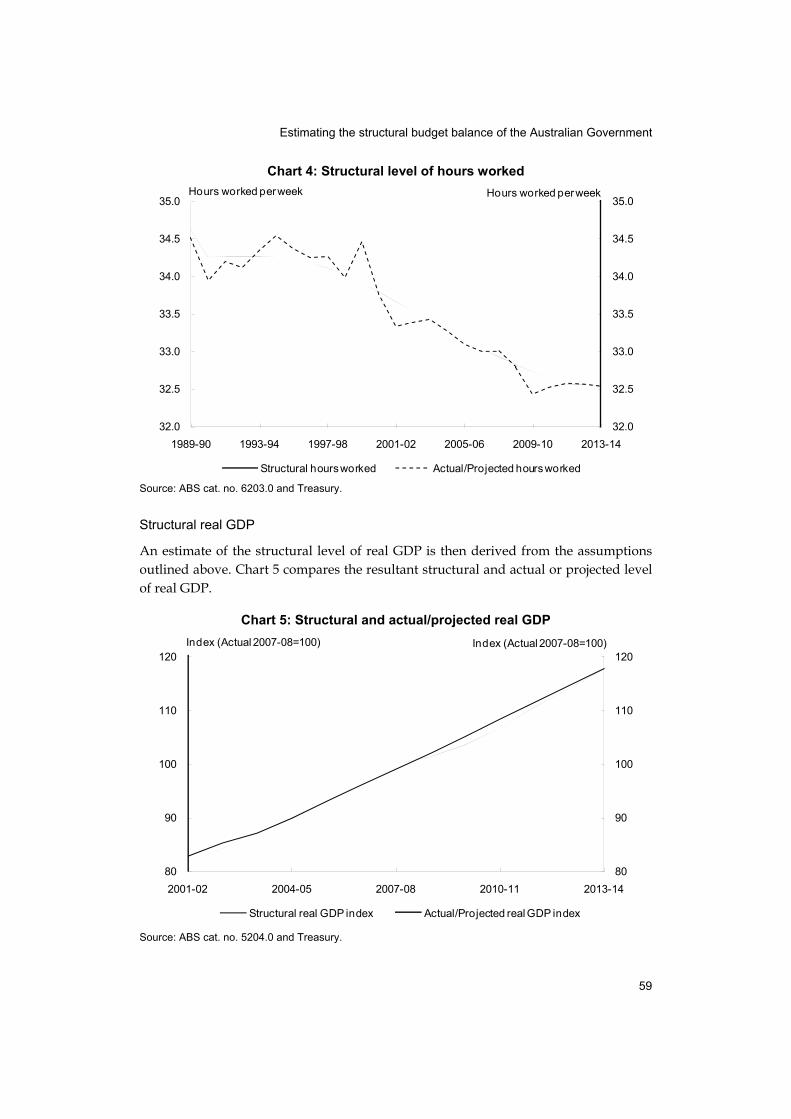
In practice, it is difficult to separate any cyclical factors affecting average hours worked per employee from these structural changes. The approach adopted was to assume the structural level of hours worked per employee equalled the trend level derived from a Hodrick-Prescott filter, with any variation from this trend assumed to reflect cyclical factors (Chart 4).


59

Chart 4: Structural level of hours worked

32.0

32.5

33.0

33.5

34.0

34.5

35.0

32.0

32.5

33.0

33.5

34.0

34.5

35.0

1989-90 1993-94 1997-98 2001-02 2005-06 2009-10 2013-14

Structural hours worked Actual/Projected hours worked

Hours worked per week Hours worked per week


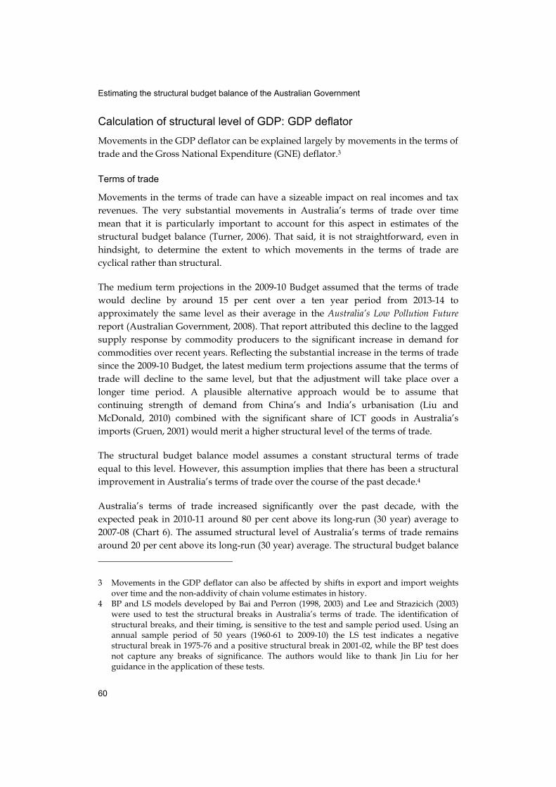
Structural real GDP

An estimate of the structural level of real GDP is then derived from the assumptions outlined above. Chart 5 compares the resultant structural and actual or projected level of real GDP.

Chart 5: Structural and actual/projected real GDP

80

90

100

110

120

80

90

100

110

120

2001-02 2004-05 2007-08 2010-11 2013-14

Structural real GDP index Actual/Projected real GDP index

Index (Actual 2007-08=100) Index (Actual 2007-08=100)



60

Calculation of structural level of GDP: GDP deflator

Movements in the GDP deflator can be explained largely by movements in the terms of trade and the Gross National Expenditure (GNE) deflator.3

Terms of trade

Movements in the terms of trade can have a sizeable impact on real incomes and tax revenues. The very substantial movements in Australia’s terms of trade over time mean that it is particularly important to account for this aspect in estimates of the structural budget balance (Turner, 2006). That said, it is not straightforward, even in hindsight, to determine the extent to which movements in the terms of trade are cyclical rather than structural.

The medium term projections in the 2009-10 Budget assumed that the terms of trade would decline by around 15 per cent over a ten year period from 2013-14 to approximately the same level as their average in the Australia’s Low Pollution Future report (Australian Government, 2008). That report attributed this decline to the lagged supply response by commodity producers to the significant increase in demand for commodities over recent years. Reflecting the substantial increase in the terms of trade since the 2009-10 Budget, the latest medium term projections assume that the terms of trade will decline to the same level, but that the adjustment will take place over a longer time period. A plausible alternative approach would be to assume that continuing strength of demand from China’s and India’s urbanisation (Liu and McDonald, 2010) combined with the significant share of ICT goods in Australia’s imports (Gruen, 2001) would merit a higher structural level of the terms of trade.

The structural budget balance model assumes a constant structural terms of trade equal to this level. However, this assumption implies that there has been a structural improvement in Australia’s terms of trade over the course of the past decade.4

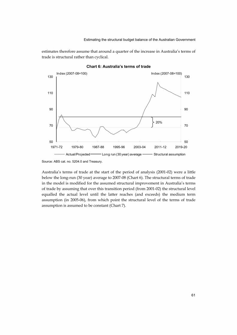
Australia’s terms of trade increased significantly over the past decade, with the expected peak in 2010-11 around 80 per cent above its long-run (30 year) average to 2007-08 (Chart 6). The assumed structural level of Australia’s terms of trade remains around 20 per cent above its long-run (30 year) average. The structural budget balance

3 Movements in the GDP deflator can also be affected by shifts in export and import weights over time and the non-addivity of chain volume estimates in history.

4 BP and LS models developed by Bai and Perron (1998, 2003) and Lee and Strazicich (2003) were used to test the structural breaks in Australia’s terms of trade. The identification of structural breaks, and their timing, is sensitive to the test and sample period used. Using an annual sample period of 50 years (1960-61 to 2009-10) the LS test indicates a negative structural break in 1975-76 and a positive structural break in 2001-02, while the BP test does not capture any breaks of significance. The authors would like to thank Jin Liu for her guidance in the application of these tests.


61

estimates therefore assume that around a quarter of the increase in Australia’s terms of trade is structural rather than cyclical.

Chart 6: Australia’s terms of trade

50

70

90

110

130

50

70

90

110

130

1971-72 1979-80 1987-88 1995-96 2003-04 2011-12 2019-20

Actual/Projected Long run (30 year) average Structural assumption

Index (2007-08=100) Index (2007-08=100)

20%


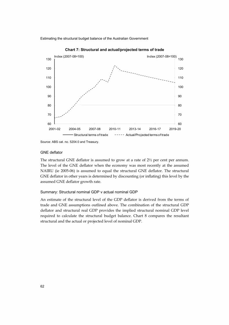
Australia’s terms of trade at the start of the period of analysis (2001-02) were a little below the long-run (30 year) average to 2007-08 (Chart 6). The structural terms of trade in the model is modified for the assumed structural improvement in Australia’s terms of trade by assuming that over this transition period (from 2001-02) the structural level equalled the actual level until the latter reaches (and exceeds) the medium term assumption (in 2005-06), from which point the structural level of the terms of trade assumption is assumed to be constant (Chart 7).


62

Chart 7: Structural and actual/projected terms of trade

60

70

80

90

100

110

120

130

60

70

80

90

100

110

120

130

2001-02 2004-05 2007-08 2010-11 2013-14 2016-17 2019-20

Structural terms of trade Actual/Projected terms of trade

Index (2007-08=100) Index (2007-08=100)


GNE deflator

The structural GNE deflator is assumed to grow at a rate of 2½ per cent per annum. The level of the GNE deflator when the economy was most recently at the assumed NAIRU (ie 2005-06) is assumed to equal the structural GNE deflator. The structural GNE deflator in other years is determined by discounting (or inflating) this level by the assumed GNE deflator growth rate.

Summary: Structural nominal GDP v actual nominal GDP

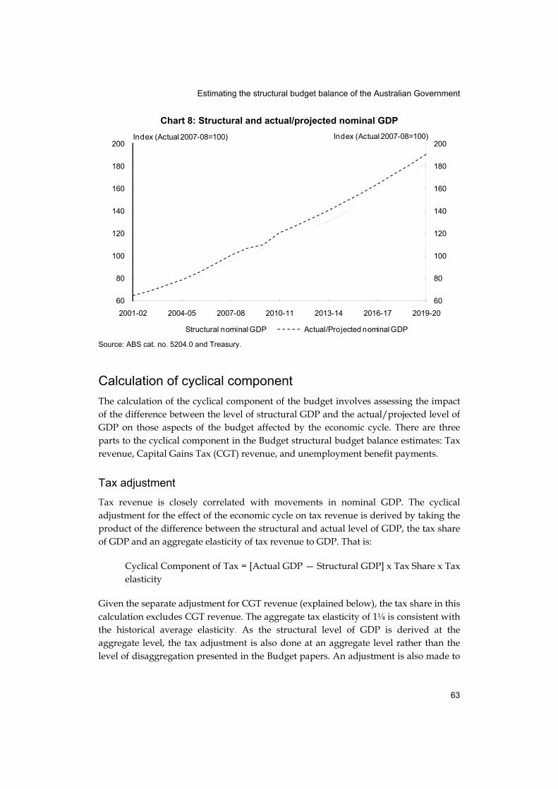
An estimate of the structural level of the GDP deflator is derived from the terms of trade and GNE assumptions outlined above. The combination of the structural GDP deflator and structural real GDP provides the implied structural nominal GDP level required to calculate the structural budget balance. Chart 8 compares the resultant structural and the actual or projected level of nominal GDP.


63

Chart 8: Structural and actual/projected nominal GDP

60

80

100

120

140

160

180

200

60

80

100

120

140

160

180

200

2001-02 2004-05 2007-08 2010-11 2013-14 2016-17 2019-20

Structural nominal GDP Actual/Projected nominal GDP

Index (Actual 2007-08=100) Index (Actual 2007-08=100)


Calculation of cyclical component

The calculation of the cyclical component of the budget involves assessing the impact of the difference between the level of structural GDP and the actual/projected level of GDP on those aspects of the budget affected by the economic cycle. There are three parts to the cyclical component in the Budget structural budget balance estimates: Tax revenue, Capital Gains Tax (CGT) revenue, and unemployment benefit payments.

Tax adjustment

Tax revenue is closely correlated with movements in nominal GDP. The cyclical adjustment for the effect of the economic cycle on tax revenue is derived by taking the product of the difference between the structural and actual level of GDP, the tax share of GDP and an aggregate elasticity of tax revenue to GDP. That is:

Cyclical Component of Tax = [Actual GDP — Structural GDP] x Tax Share x Tax elasticity

Given the separate adjustment for CGT revenue (explained below), the tax share in this calculation excludes CGT revenue. The aggregate tax elasticity of 1¼ is consistent with the historical average elasticity. As the structural level of GDP is derived at the aggregate level, the tax adjustment is also done at an aggregate level rather than the level of disaggregation presented in the Budget papers. An adjustment is also made to


64

reflect the lags from changes in economic conditions to tax revenue. Around 80 per cent of the impact is assumed to occur in the year of the change, with around 20 per cent in the following year.

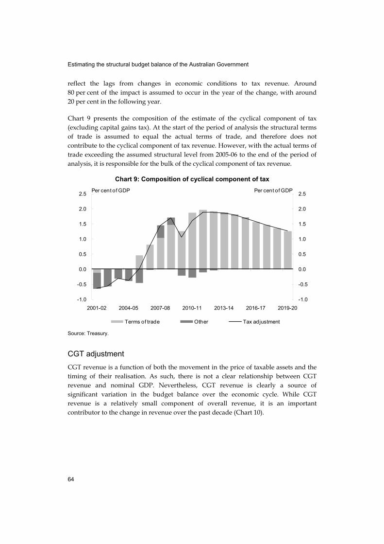
Chart 9 presents the composition of the estimate of the cyclical component of tax (excluding capital gains tax). At the start of the period of analysis the structural terms of trade is assumed to equal the actual terms of trade, and therefore does not contribute to the cyclical component of tax revenue. However, with the actual terms of trade exceeding the assumed structural level from 2005-06 to the end of the period of analysis, it is responsible for the bulk of the cyclical component of tax revenue.

Chart 9: Composition of cyclical component of tax

-1.0

-0.5

0.0

0.5

1.0

1.5

2.0

2.5

-1.0

-0.5

0.0

0.5

1.0

1.5

2.0

2.5

2001-02 2004-05 2007-08 2010-11 2013-14 2016-17 2019-20

Terms of trade Other Tax adjustment

Per cent of GDP Per cent of GDP

Source: Treasury.

CGT adjustment

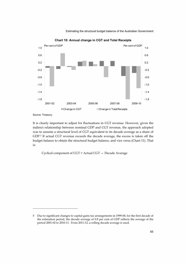
CGT revenue is a function of both the movement in the price of taxable assets and the timing of their realisation. As such, there is not a clear relationship between CGT revenue and nominal GDP. Nevertheless, CGT revenue is clearly a source of significant variation in the budget balance over the economic cycle. While CGT revenue is a relatively small component of overall revenue, it is an important contributor to the change in revenue over the past decade (Chart 10).


65

Chart 10: Annual change in CGT and Total Receipts

-1.8

-1.4

-1.0

-0.6

-0.2

0.2

0.6

1.0

-1.8

-1.4

-1.0

-0.6

-0.2

0.2

0.6

1.0

2001-02 2003-04 2005-06 2007-08 2009-10

Change in CGT Change in Total Receipts


Source: Treasury.

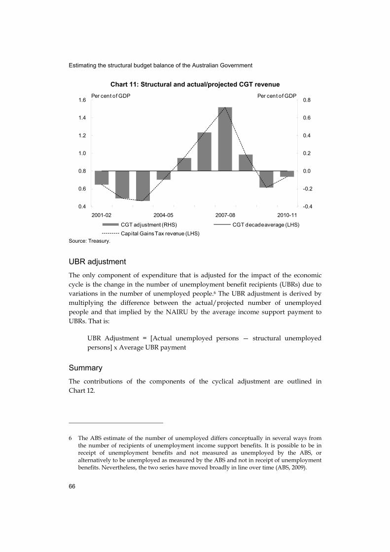
It is clearly important to adjust for fluctuations in CGT revenue. However, given the indirect relationship between nominal GDP and CGT revenue, the approach adopted was to assume a structural level of CGT equivalent to its decade average as a share of GDP.5 If actual CGT revenue exceeds the decade average, the excess is taken off the budget balance to obtain the structural budget balance, and vice versa (Chart 11). That is:

Cyclical component of CGT = Actual CGT — Decade Average

5 Due to significant changes to capital gains tax arrangements in 1999-00, for the first decade of the estimation period, the decade average of 0.8 per cent of GDP reflects the average of the period 2001-02 to 2010-11. From 2011-12, a rolling decade average is used.


66

Chart 11: Structural and actual/projected CGT revenue

-0.4

-0.2

0.0

0.2

0.4

0.6

0.8

0.4

0.6

0.8

1.0

1.2

1.4

1.6

2001-02 2004-05 2007-08 2010-11

CGT adjustment (RHS) CGT decade average (LHS)

Capital Gains Tax revenue (LHS)


Source: Treasury.

UBR adjustment

The only component of expenditure that is adjusted for the impact of the economic cycle is the change in the number of unemployment benefit recipients (UBRs) due to variations in the number of unemployed people.6 The UBR adjustment is derived by multiplying the difference between the actual/projected number of unemployed people and that implied by the NAIRU by the average income support payment to UBRs. That is:

UBR Adjustment = [Actual unemployed persons — structural unemployed persons] x Average UBR payment

Summary

The contributions of the components of the cyclical adjustment are outlined in Chart 12.

6 The ABS estimate of the number of unemployed differs conceptually in several ways from the number of recipients of unemployment income support benefits. It is possible to be in receipt of unemployment benefits and not measured as unemployed by the ABS, or alternatively to be unemployed as measured by the ABS and not in receipt of unemployment benefits. Nevertheless, the two series have moved broadly in line over time (ABS, 2009).


67

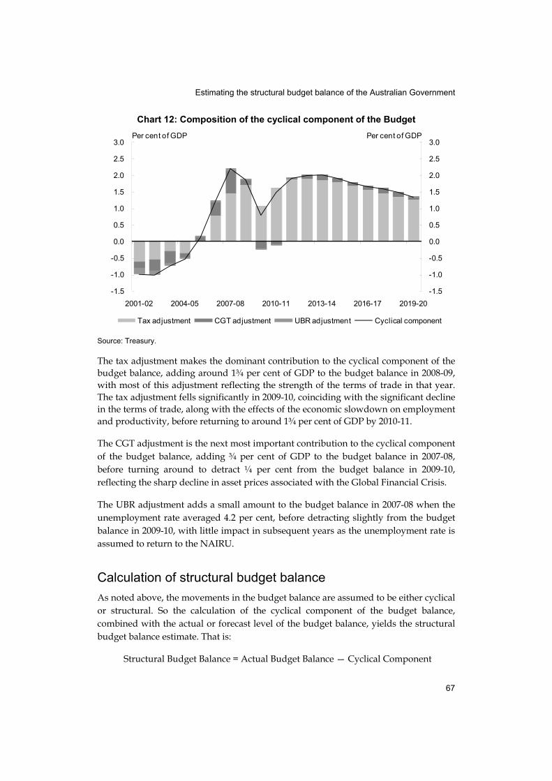
Chart 12: Composition of the cyclical component of the Budget

-1.5

-1.0

-0.5

0.0

0.5

1.0

1.5

2.0

2.5

3.0

-1.5

-1.0

-0.5

0.0

0.5

1.0

1.5

2.0

2.5

3.0

2001-02 2004-05 2007-08 2010-11 2013-14 2016-17 2019-20

Tax adjustment CGT adjustment UBR adjustment Cyclical component


Source: Treasury. The tax adjustment makes the dominant contribution to the cyclical component of the budget balance, adding around 1¾ per cent of GDP to the budget balance in 2008-09, with most of this adjustment reflecting the strength of the terms of trade in that year. The tax adjustment fells significantly in 2009-10, coinciding with the significant decline in the terms of trade, along with the effects of the economic slowdown on employment and productivity, before returning to around 1¾ per cent of GDP by 2010-11.

The CGT adjustment is the next most important contribution to the cyclical component of the budget balance, adding ¾ per cent of GDP to the budget balance in 2007-08, before turning around to detract ¼ per cent from the budget balance in 2009-10, reflecting the sharp decline in asset prices associated with the Global Financial Crisis.

The UBR adjustment adds a small amount to the budget balance in 2007-08 when the unemployment rate averaged 4.2 per cent, before detracting slightly from the budget balance in 2009-10, with little impact in subsequent years as the unemployment rate is assumed to return to the NAIRU.

Calculation of structural budget balance

As noted above, the movements in the budget balance are assumed to be either cyclical or structural. So the calculation of the cyclical component of the budget balance, combined with the actual or forecast level of the budget balance, yields the structural budget balance estimate. That is:

Structural Budget Balance = Actual Budget Balance — Cyclical Component


68

The above terms are expressed in terms of a percentage of GDP.7

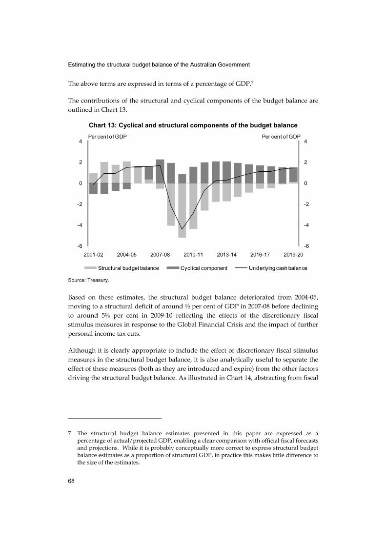
The contributions of the structural and cyclical components of the budget balance are outlined in Chart 13.

Chart 13: Cyclical and structural components of the budget balance

-6

-4

-2

0

2

4

-6

-4

-2

0

2

4

2001-02 2004-05 2007-08 2010-11 2013-14 2016-17 2019-20

Structural budget balance Cyclical component Underlying cash balance


Source: Treasury.

Based on these estimates, the structural budget balance deteriorated from 2004-05, moving to a structural deficit of around ½ per cent of GDP in 2007-08 before declining to around 5¼ per cent in 2009-10 reflecting the effects of the discretionary fiscal stimulus measures in response to the Global Financial Crisis and the impact of further personal income tax cuts.

Although it is clearly appropriate to include the effect of discretionary fiscal stimulus measures in the structural budget balance, it is also analytically useful to separate the effect of these measures (both as they are introduced and expire) from the other factors driving the structural budget balance. As illustrated in Chart 14, abstracting from fiscal

7 The structural budget balance estimates presented in this paper are expressed as a percentage of actual/projected GDP, enabling a clear comparison with official fiscal forecasts and projections. While it is probably conceptually more correct to express structural budget balance estimates as a proportion of structural GDP, in practice this makes little difference to the size of the estimates.


69

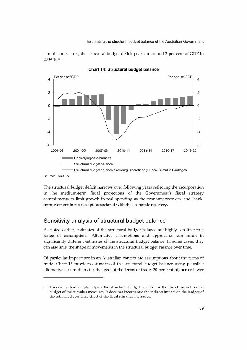
stimulus measures, the structural budget deficit peaks at around 3 per cent of GDP in 2009-10.8

Chart 14: Structural budget balance

-6

-4

-2

0

2

4

-6

-4

-2

0

2

4

2001-02 2004-05 2007-08 2010-11 2013-14 2016-17 2019-20

Underlying cash balance

Structural budget balance

Structural budget balance excluding Discretionary Fiscal Stimulus Packages


Source: Treasury.

The structural budget deficit narrows over following years reflecting the incorporation in the medium-term fiscal projections of the Government’s fiscal strategy commitments to limit growth in real spending as the economy recovers, and ‘bank’ improvement in tax receipts associated with the economic recovery.

Sensitivity analysis of structural budget balance

As noted earlier, estimates of the structural budget balance are highly sensitive to a range of assumptions. Alternative assumptions and approaches can result in significantly different estimates of the structural budget balance. In some cases, they can also shift the shape of movements in the structural budget balance over time.

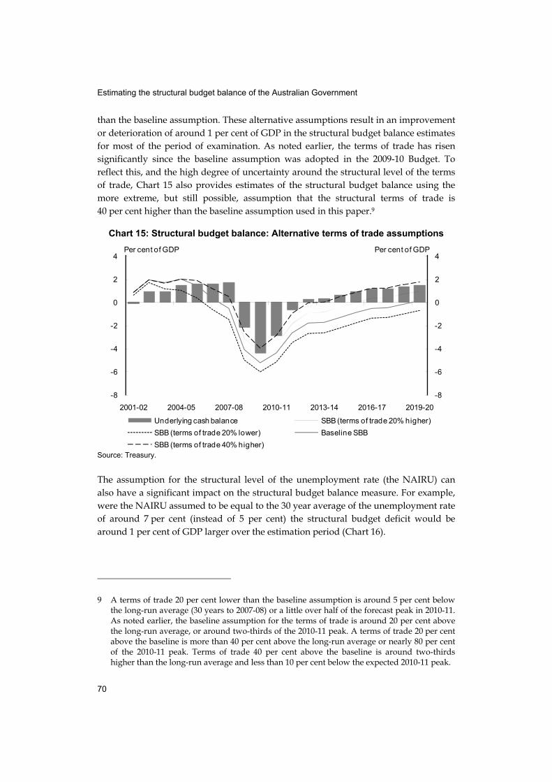
Of particular importance in an Australian context are assumptions about the terms of trade. Chart 15 provides estimates of the structural budget balance using plausible alternative assumptions for the level of the terms of trade: 20 per cent higher or lower

8 This calculation simply adjusts the structural budget balance for the direct impact on the budget of the stimulus measures. It does not incorporate the indirect impact on the budget of the estimated economic effect of the fiscal stimulus measures.


70

than the baseline assumption. These alternative assumptions result in an improvement or deterioration of around 1 per cent of GDP in the structural budget balance estimates for most of the period of examination. As noted earlier, the terms of trade has risen significantly since the baseline assumption was adopted in the 2009-10 Budget. To reflect this, and the high degree of uncertainty around the structural level of the terms of trade, Chart 15 also provides estimates of the structural budget balance using the more extreme, but still possible, assumption that the structural terms of trade is 40 per cent higher than the baseline assumption used in this paper.9

Chart 15: Structural budget balance: Alternative terms of trade assumptions

-8

-6

-4

-2

0

2

4

-8

-6

-4

-2

0

2

4

2001-02 2004-05 2007-08 2010-11 2013-14 2016-17 2019-20

Underlying cash balance SBB (terms of trade 20% higher)

SBB (terms of trade 20% lower) Baseline SBB

SBB (terms of trade 40% higher)


Source: Treasury.

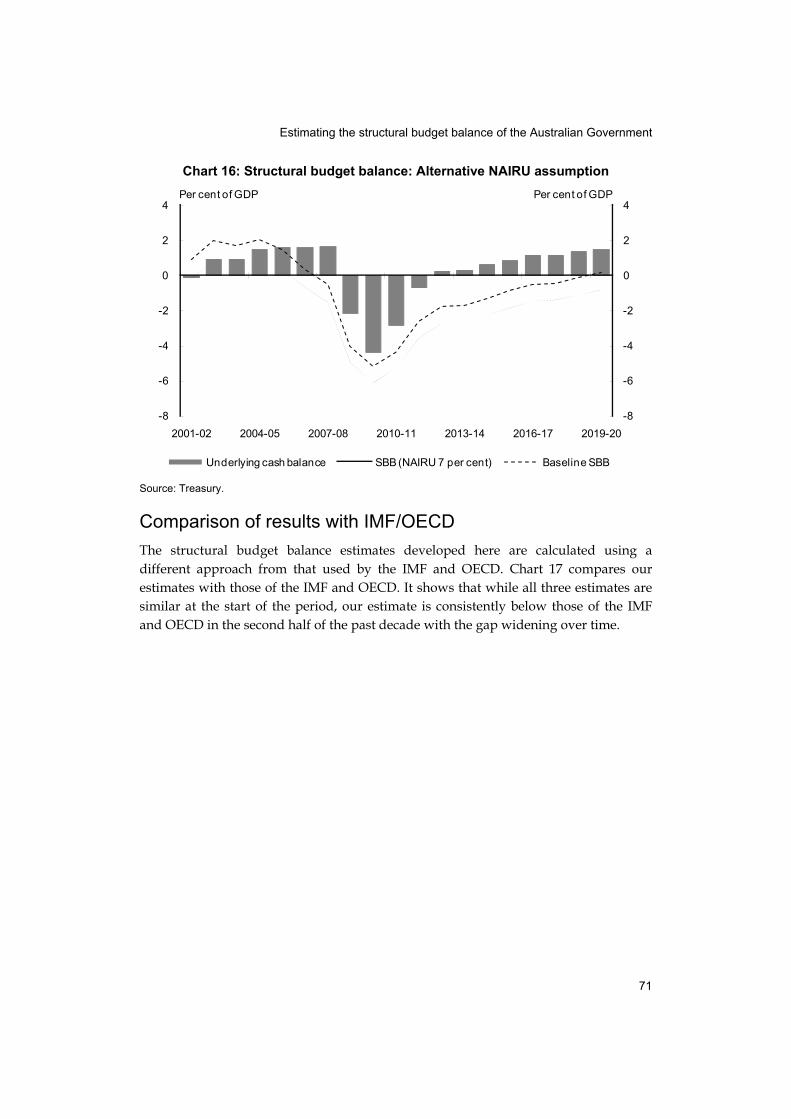
The assumption for the structural level of the unemployment rate (the NAIRU) can also have a significant impact on the structural budget balance measure. For example, were the NAIRU assumed to be equal to the 30 year average of the unemployment rate of around 7 per cent (instead of 5 per cent) the structural budget deficit would be around 1 per cent of GDP larger over the estimation period (Chart 16).

9 A terms of trade 20 per cent lower than the baseline assumption is around 5 per cent below the long-run average (30 years to 2007-08) or a little over half of the forecast peak in 2010-11. As noted earlier, the baseline assumption for the terms of trade is around 20 per cent above the long-run average, or around two-thirds of the 2010-11 peak. A terms of trade 20 per cent above the baseline is more than 40 per cent above the long-run average or nearly 80 per cent of the 2010-11 peak. Terms of trade 40 per cent above the baseline is around two-thirds higher than the long-run average and less than 10 per cent below the expected 2010-11 peak.


71

Chart 16: Structural budget balance: Alternative NAIRU assumption

-8

-6

-4

-2

0

2

4

-8

-6

-4

-2

0

2

4

2001-02 2004-05 2007-08 2010-11 2013-14 2016-17 2019-20

Underlying cash balance SBB (NAIRU 7 per cent) Baseline SBB


Source: Treasury.

Comparison of results with IMF/OECD

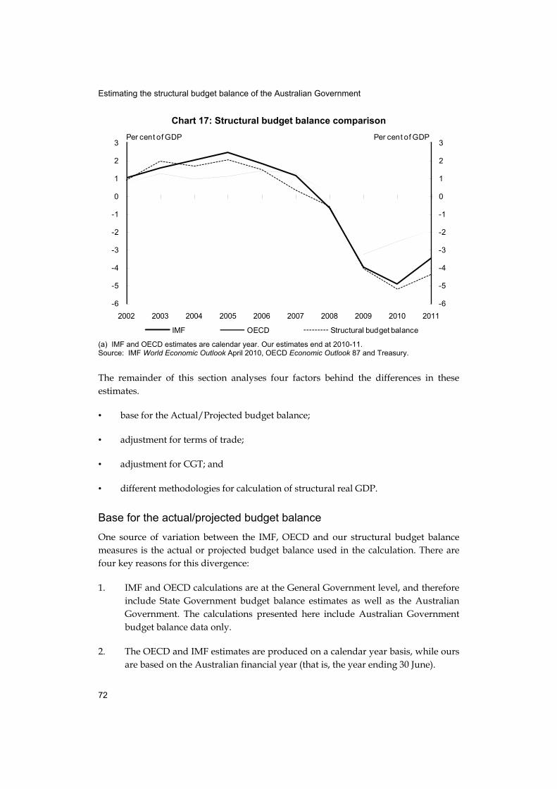
The structural budget balance estimates developed here are calculated using a different approach from that used by the IMF and OECD. Chart 17 compares our estimates with those of the IMF and OECD. It shows that while all three estimates are similar at the start of the period, our estimate is consistently below those of the IMF and OECD in the second half of the past decade with the gap widening over time.


72

Chart 17: Structural budget balance comparison

-6

-5

-4

-3

-2

-1

0

1

2

3

-6

-5

-4

-3

-2

-1

0

1

2

3

2002 2003 2004 2005 2006 2007 2008 2009 2010 2011

IMF OECD Structural budget balance


(a) IMF and OECD estimates are calendar year. Our estimates end at 2010-11. Source: IMF World Economic Outlook April 2010, OECD Economic Outlook 87 and Treasury.

The remainder of this section analyses four factors behind the differences in these estimates.

• base for the Actual/Projected budget balance;

• adjustment for terms of trade;

• adjustment for CGT; and

• different methodologies for calculation of structural real GDP.

Base for the actual/projected budget balance

One source of variation between the IMF, OECD and our structural budget balance measures is the actual or projected budget balance used in the calculation. There are four key reasons for this divergence:

1. IMF and OECD calculations are at the General Government level, and therefore include State Government budget balance estimates as well as the Australian Government. The calculations presented here include Australian Government budget balance data only.

2. The OECD and IMF estimates are produced on a calendar year basis, while ours are based on the Australian financial year (that is, the year ending 30 June).


73

3. The OECD and IMF estimates use the underlying primary budget balance, while ours use the underlying cash balance measure.

4. The estimates of the budget balance are produced at slightly different times and therefore incorporate different information about the state of the economy and the fiscal decisions of the Government. The IMF estimates were published in the World Economic Outlook in April 2010 (before the 2010-11 Budget), while the latest OECD estimates were published in the Economic Outlook released in June 2010, post-Budget. As noted earlier, our estimates are based on the state of the economy, and economic forecasts, from the Pre-Election Economic and Fiscal Outlook, published in July 2010.

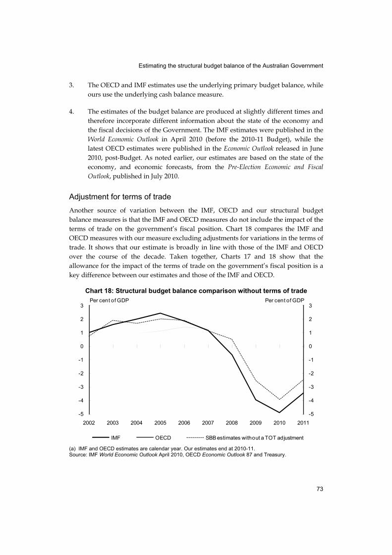
Adjustment for terms of trade

Another source of variation between the IMF, OECD and our structural budget balance measures is that the IMF and OECD measures do not include the impact of the terms of trade on the government’s fiscal position. Chart 18 compares the IMF and OECD measures with our measure excluding adjustments for variations in the terms of trade. It shows that our estimate is broadly in line with those of the IMF and OECD over the course of the decade. Taken together, Charts 17 and 18 show that the allowance for the impact of the terms of trade on the government’s fiscal position is a key difference between our estimates and those of the IMF and OECD.

Chart 18: Structural budget balance comparison without terms of trade

-5

-4

-3

-2

-1

0

1

2

3

-5

-4

-3

-2

-1

0

1

2

3

2002 2003 2004 2005 2006 2007 2008 2009 2010 2011

IMF OECD SBB estimates without a TOT adjustment




74

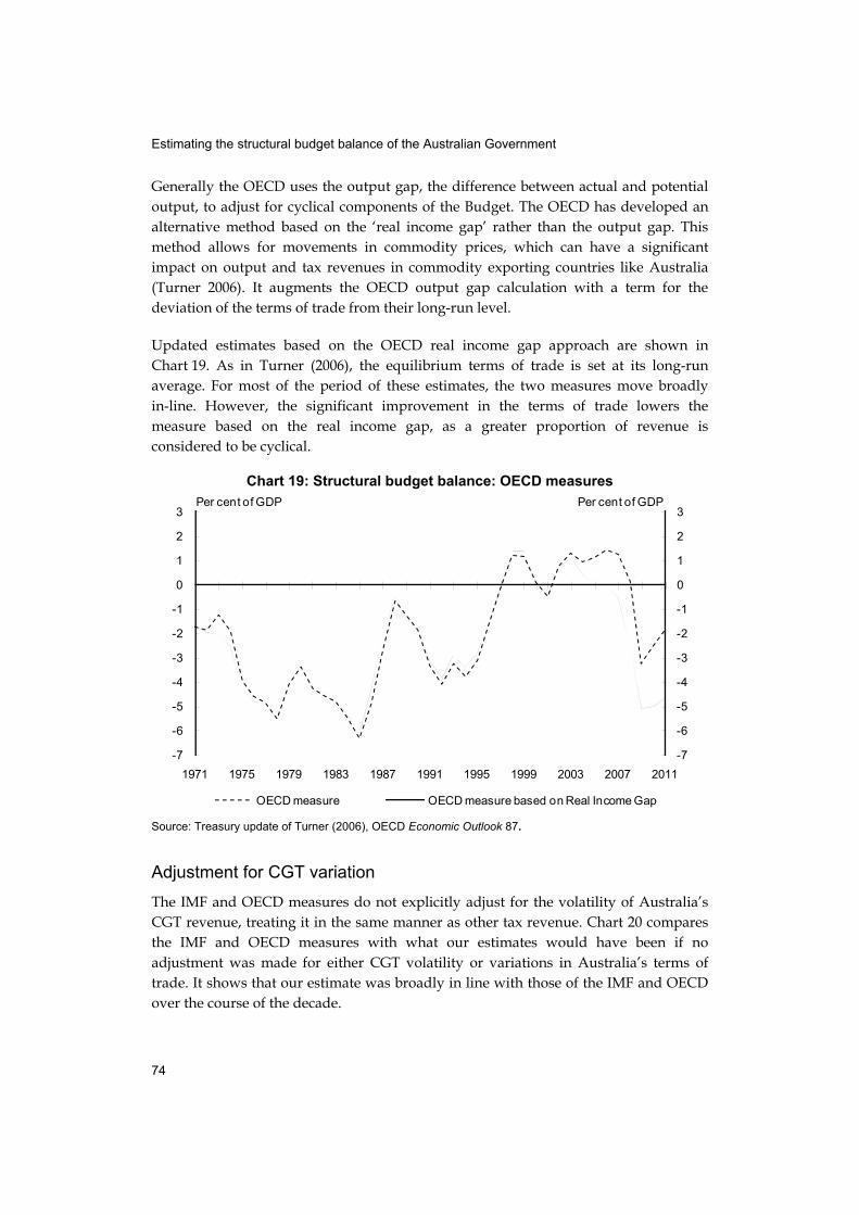
Generally the OECD uses the output gap, the difference between actual and potential output, to adjust for cyclical components of the Budget. The OECD has developed an alternative method based on the ‘real income gap’ rather than the output gap. This method allows for movements in commodity prices, which can have a significant impact on output and tax revenues in commodity exporting countries like Australia (Turner 2006). It augments the OECD output gap calculation with a term for the deviation of the terms of trade from their long-run level.

Updated estimates based on the OECD real income gap approach are shown in Chart 19. As in Turner (2006), the equilibrium terms of trade is set at its long-run average. For most of the period of these estimates, the two measures move broadly in-line. However, the significant improvement in the terms of trade lowers the measure based on the real income gap, as a greater proportion of revenue is considered to be cyclical.

Chart 19: Structural budget balance: OECD measures

-7

-6

-5

-4

-3

-2

-1

0

1

2

3

-7

-6

-5

-4

-3

-2

-1

0

1

2

3

1971 1975 1979 1983 1987 1991 1995 1999 2003 2007 2011

OECD measure OECD measure based on Real Income Gap


Source: Treasury update of Turner (2006), OECD Economic Outlook 87.

Adjustment for CGT variation

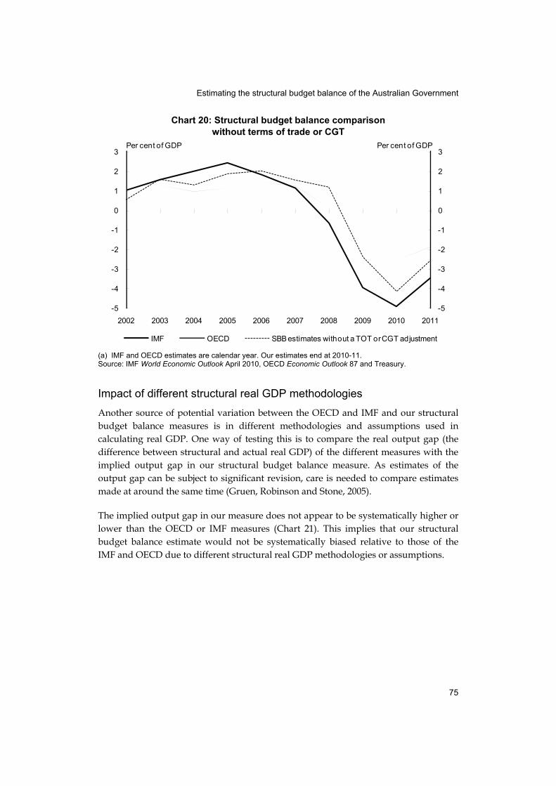
The IMF and OECD measures do not explicitly adjust for the volatility of Australia’s CGT revenue, treating it in the same manner as other tax revenue. Chart 20 compares the IMF and OECD measures with what our estimates would have been if no adjustment was made for either CGT volatility or variations in Australia’s terms of trade. It shows that our estimate was broadly in line with those of the IMF and OECD over the course of the decade.


75

Chart 20: Structural budget balance comparison without terms of trade or CGT

-5

-4

-3

-2

-1

0

1

2

3

-5

-4

-3

-2

-1

0

1

2

3

2002 2003 2004 2005 2006 2007 2008 2009 2010 2011

IMF OECD SBB estimates without a TOT or CGT adjustment



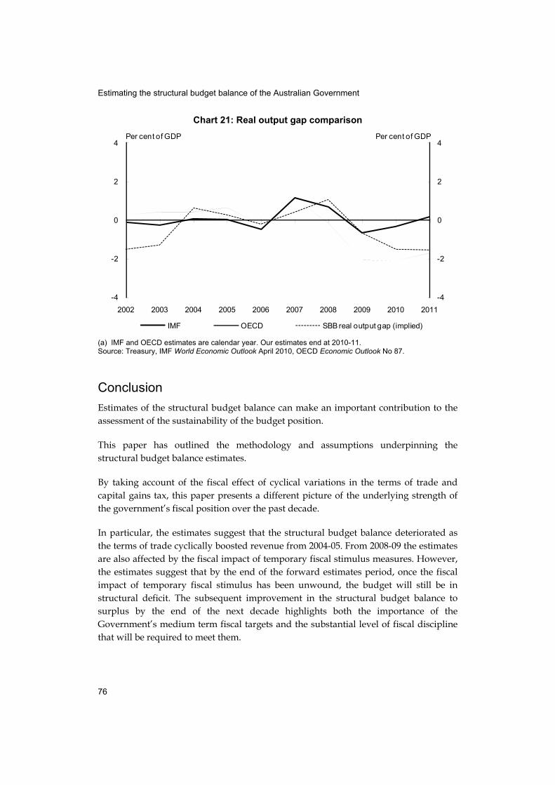
Impact of different structural real GDP methodologies

Another source of potential variation between the OECD and IMF and our structural budget balance measures is in different methodologies and assumptions used in calculating real GDP. One way of testing this is to compare the real output gap (the difference between structural and actual real GDP) of the different measures with the implied output gap in our structural budget balance measure. As estimates of the output gap can be subject to significant revision, care is needed to compare estimates made at around the same time (Gruen, Robinson and Stone, 2005).

The implied output gap in our measure does not appear to be systematically higher or lower than the OECD or IMF measures (Chart 21). This implies that our structural budget balance estimate would not be systematically biased relative to those of the IMF and OECD due to different structural real GDP methodologies or assumptions.


76

Chart 21: Real output gap comparison

-4

-2

0

2

4

-4

-2

0

2

4

2002 2003 2004 2005 2006 2007 2008 2009 2010 2011

IMF OECD SBB real output gap (implied)


(a) IMF and OECD estimates are calendar year. Our estimates end at 2010-11. Source: Treasury, IMF World Economic Outlook April 2010, OECD Economic Outlook No 87.

Conclusion

Estimates of the structural budget balance can make an important contribution to the assessment of the sustainability of the budget position.

This paper has outlined the methodology and assumptions underpinning the structural budget balance estimates.

By taking account of the fiscal effect of cyclical variations in the terms of trade and capital gains tax, this paper presents a different picture of the underlying strength of the government’s fiscal position over the past decade.

In particular, the estimates suggest that the structural budget balance deteriorated as the terms of trade cyclically boosted revenue from 2004-05. From 2008-09 the estimates are also affected by the fiscal impact of temporary fiscal stimulus measures. However, the estimates suggest that by the end of the forward estimates period, once the fiscal impact of temporary fiscal stimulus has been unwound, the budget will still be in structural deficit. The subsequent improvement in the structural budget balance to surplus by the end of the next decade highlights both the importance of the Government’s medium term fiscal targets and the substantial level of fiscal discipline that will be required to meet them.


77

The paper also highlights the range of plausible approaches and assumptions that could have a material effect on estimates the structural budget balance. This highlights the importance of being mindful of the limitations of these measures when interpreting their results.

In particular, the estimates in this paper are heavily influenced by assumptions around the equilibrium terms of trade – that is, the extent to which improvements in the terms of trade over the decade are structural rather than cyclical. Alternative assumptions about the equilibrium terms of trade result in significantly different structural budget balance estimates. This cautions against excessive reliance on point estimates of the structural budget balance derived by any particular approach, including those presented here. Rather, these estimates are best considered as one input into a broad assessment of fiscal sustainability.


78

References

Australian Bureau of Statistics, 2009, ‘Comparing Unemployment and the Claimant Count’ 6105.0 — Australian Labour Market Statistics, Jan 2009.

Australian Government, 2008, Australia’s Low Pollution Future: The Economics of Climate Change Mitigation, Canberra.

Bai, J and Perron, P 1998, ‘Estimating and Testing Liner Models with Multiples Structural Changes’, Econometrica, 66, 47-78.

Bai, J and Perron, P 2003, ‘Computation and Analysis of Multiple Structural Change Models’, Journal of Applied Econometrics, 18, 1-22.

Chalk, N 2002, ‘Structural Balances and all that: Which Indicators to Use in Assessing Fiscal Policy’, IMF Working Paper 02/101, International Monetary Fund, Washington DC.

Commonwealth of Australia, 2009, Budget Paper No. 1, Canberra.

De Masi, PR 1997, ‘IMF Estimates of Potential Output: Theory and Practice’, IMF Working Paper 97/177, International Monetary Fund, Washington DC.

Fedelino, A, Ivanova, A and Horton, M, ‘Computing Cyclically Adjusted Balances and Automatic Stabilisers’, IMF Technical Notes and Manuals 09/05, International Monetary Fund, Washington DC.

Ford, B 2005, ‘Structural Fiscal Indicators: an overview’, Economic Roundup, Autumn, Treasury, Canberra.

Giorno, C, Richardson, P, Roseveare, D and van den Noord, P 1995, ‘Potential Output, Output Gaps and Structural Budget Balances’, OECD Economic Studies, No. 24, Paris.

Girouard, N and Andre, C, 2005, ‘Measuring Cyclically-adjusted Budget Balances for OECD countries’, OECD Economics Department Working Papers, No 434.

Gruen, D, 2001, ‘Some Possible Long-term Trends in the Australian Dollar’, Reserve Bank of Australia Bulletin, December, 30-41.

Gruen, D, Robinson, T and Stone, A 2005, ‘Output Gaps in Real Time: How Reliable Are They?’, Economic Record, 81, 6-18.

Gruen, D and Sayegh, A 2005, ‘The Evolution of Fiscal Policy in Australia’, Oxford Review of Economic Policy, 21, Oxford University Press.


79

Hagemann, R 1999, ‘The Structural Budget Balance: The IMF’s Methodology’, IMF Working Paper 99/95, International Monetary Fund, Washington DC.

Henry, K 2001, ‘Australia’s Economic Development: Address to The Committee for The Economic Development of Australia’, Economic Roundup, Spring, Treasury, Canberra.

IMF 2009, World Economic Outlook Report, October, IMF, Washington DC.

Lee, J and Strazicich, C 2003, ‘Minimum Lagrange Multiplier Unit Root Test with Two Structural Breaks, The Review of Economics and Statistics, 85, 1082-1089.

Liu, J and McDonald, T, 2010, ‘China: growth, urbanisation and mineral resource demand’, Economic Roundup, Issue 2, Treasury, Canberra.

Koske, I and Pain, N 2008, ‘The Usefulness of Output Gaps for Policy Analysis’, OECD Economics Department Working Paper, no 621, OECD, Paris.

Mercereau, B and Razhkov, D 2006, ‘Fiscal Policy and the Terms of Trade Boom’, IMF Country Report No. 06/373, International Monetary Fund, Washington DC.

OECD 2009, Economic Outlook No 86, OECD, Paris.

Price, B, Joumard, I, Andre C, and Minegishi, M 2008 ‘Strategies for Countries with Favourable Fiscal Positions’, OECD Economics Department, Working Paper No. 655.

Roger, W and Ongena, H 1999, ‘The Commission’s Cyclical Adjustment Method’, Paper presented at Bank of Italy Workshop, Perugia, 26-28 November 1998.

Suyker, W 1999, ‘Structural Budget Balances: The Method Applied by the OECD’, Paper presented at Bank of Italy Workshop, Perugia, 26-28 November 1998.

Treasury, 2000, ‘Demographic Influences on Long-term Economic Growth in Australia’, Economic Roundup, Winter, Canberra.

Turner, D 2006, ‘Should Measures of Fiscal Stance be Adjusted for Terms of Trade Effects’, Economics Department Working Paper, No. 519, OECD, Paris.

Van den Noord, P 2000, ‘The Size and Role of Automatic Fiscal Stabilisers in the 1990s and Beyond’, OECD Economics Department Working Papers, No. 230, OECD, Paris.

Woods, D, Farrugia, M and Pirie, M. 2009, ‘The Australian Treasury’s fiscal aggregate projection model’, Economic Roundup, Issue 3, Treasury, Canberra.

Documents

Economic Roundup Issue 3, 2010 - Estimating the structural ...archive.treasury.gov.au/documents/1881/PDF/04_Structural_Budget... · benefited from comments and ... structural and