Embed Size (px)
Citation preview
ECONOMICS
LOCAL EMPLOYMENT IMPACT FROM COMPETING ENERGY SOURCES: SHALE GAS
VERSUS WIND GENERATION IN TEXAS
by
Peter R Hartley Rice University and
University of Western Australia
Kenneth B Medlock III Rice University
Ted Temzelides Rice University
Xinya Zhang
Rice University
DISCUSSION PAPER 14.15
Local Employment Impact from Competing
Energy Sources: Shale Gas versus Wind
Generation in Texas∗
Peter Hartley† Kenneth B. Medlock III‡ Ted Temzelides§
Xinya Zhang¶
March 14, 2014
∗Earlier versions of this paper have been presented at the Baker Institute for Public Policy, Rice Universityand at the July 2013 USAEE meetings in Anchorage, Alaska. We thank participants for their commentsand suggestions.†Department of Economics, Rice University and Economics Department, University of Western Australia
Business School‡James A. Baker III Institute for Public Policy, Rice University§Department of Economics, Rice University¶Department of Economics, Rice University
1
DISCUSSION PAPER 14.15
Abstract
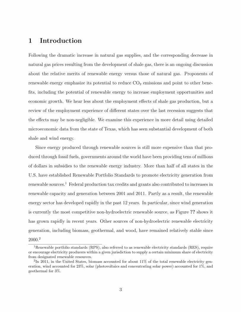
The rapid development of both wind power and of shale gas has been receiving significant
attention both in the media and among policy makers. Since these are competing sources
of electricity generation, it is informative to investigate their relative merits regarding job
creation. We use a panel econometric model to estimate the historical job-creating perfor-
mance of wind versus that of shale oil and gas. The model is estimated using monthly county
level data from Texas from 2001 to 2011. Both first-difference and GMM methods show that
shale-related activity has brought strong employment to Texas: 77 short-term jobs or 6.4
full-time equivalent (FTE) jobs per well. Given that 5482 new directional/fractured wells
were drilled in Texas in 2011, this implies that about 35000 FTE jobs were created in that
year alone. We did not, however, find a corresponding impact on wages. Our estimations
did not identify a non-negligible impact from the wind industry on either employment or
wages.
2
1 Introduction
Following the dramatic increase in natural gas supplies, and the corresponding decrease in
natural gas prices resulting from the development of shale gas, there is an ongoing discussion
about the relative merits of renewable energy versus those of natural gas. Proponents of
renewable energy emphasize its potential to reduce CO2 emissions and point to other bene-
fits, including the potential of renewable energy to increase employment opportunities and
economic growth. We hear less about the employment effects of shale gas production, but a
review of the employment experience of different states over the last recession suggests that
the effects may be non-negligible. We examine this experience in more detail using detailed
microeconomic data from the state of Texas, which has seen substantial development of both
shale and wind energy.
Since energy produced through renewable sources is still more expensive than that pro-
duced through fossil fuels, governments around the world have been providing tens of millions
of dollars in subsidies to the renewable energy industry. More than half of all states in the
U.S. have established Renewable Portfolio Standards to promote electricity generation from
renewable sources.1 Federal production tax credits and grants also contributed to increases in
renewable capacity and generation between 2001 and 2011. Partly as a result, the renewable
energy sector has developed rapidly in the past 12 years. In particular, since wind generation
is currently the most competitive non-hydroelectric renewable source, as Figure ?? shows it
has grown rapidly in recent years. Other sources of non-hydroelectric renewable electricity
generation, including biomass, geothermal, and wood, have remained relatively stable since
2000.2
1Renewable portfolio standards (RPS), also referred to as renewable electricity standards (RES), requireor encourage electricity producers within a given jurisdiction to supply a certain minimum share of electricityfrom designated renewable resources.
2In 2011, in the United States, biomass accounted for about 11% of the total renewable electricity gen-eration, wind accounted for 23%, solar (photovoltaics and concentrating solar power) accounted for 1%, andgeothermal for 3%.
3
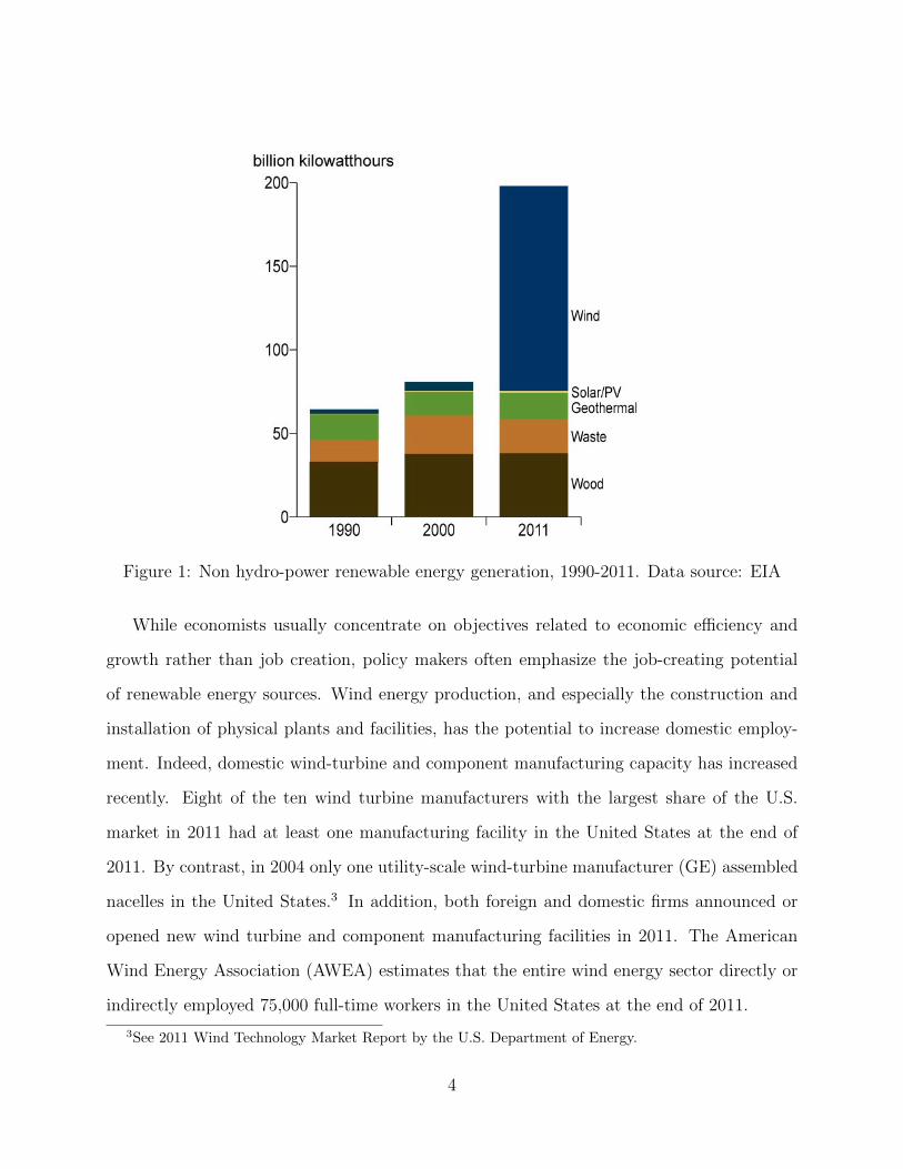
Figure 1: Non hydro-power renewable energy generation, 1990-2011. Data source: EIA
While economists usually concentrate on objectives related to economic efficiency and
growth rather than job creation, policy makers often emphasize the job-creating potential
of renewable energy sources. Wind energy production, and especially the construction and
installation of physical plants and facilities, has the potential to increase domestic employ-
ment. Indeed, domestic wind-turbine and component manufacturing capacity has increased
recently. Eight of the ten wind turbine manufacturers with the largest share of the U.S.
market in 2011 had at least one manufacturing facility in the United States at the end of
2011. By contrast, in 2004 only one utility-scale wind-turbine manufacturer (GE) assembled
nacelles in the United States.3 In addition, both foreign and domestic firms announced or
opened new wind turbine and component manufacturing facilities in 2011. The American
Wind Energy Association (AWEA) estimates that the entire wind energy sector directly or
indirectly employed 75,000 full-time workers in the United States at the end of 2011.
3See 2011 Wind Technology Market Report by the U.S. Department of Energy.
4
At the same time as wind capacity has been expanding, oil and gas companies have
demonstrated that the vast resources of shale gas and oil in North America can be exploited
at reasonable cost. This “shale revolution” is a result of cost-effective technological de-
velopments such as horizontal drilling and hydraulic fracturing. The combination of these
techniques caused U.S. production of shale oil and gas to boom.
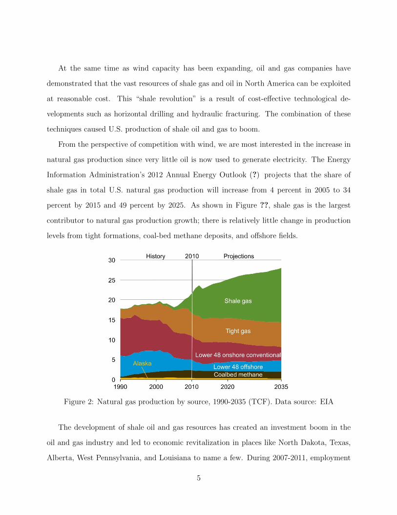
From the perspective of competition with wind, we are most interested in the increase in
natural gas production since very little oil is now used to generate electricity. The Energy
Information Administration’s 2012 Annual Energy Outlook (?) projects that the share of
shale gas in total U.S. natural gas production will increase from 4 percent in 2005 to 34
percent by 2015 and 49 percent by 2025. As shown in Figure ??, shale gas is the largest
contributor to natural gas production growth; there is relatively little change in production
levels from tight formations, coal-bed methane deposits, and offshore fields.
Figure 2: Natural gas production by source, 1990-2035 (TCF). Data source: EIA
The development of shale oil and gas resources has created an investment boom in the
oil and gas industry and led to economic revitalization in places like North Dakota, Texas,
Alberta, West Pennsylvania, and Louisiana to name a few. During 2007-2011, employment
5
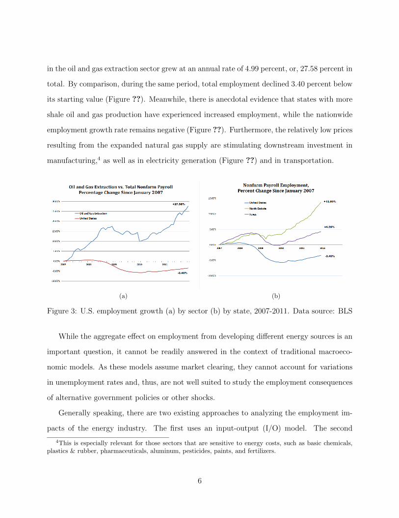
in the oil and gas extraction sector grew at an annual rate of 4.99 percent, or, 27.58 percent in
total. By comparison, during the same period, total employment declined 3.40 percent below
its starting value (Figure ??). Meanwhile, there is anecdotal evidence that states with more
shale oil and gas production have experienced increased employment, while the nationwide
employment growth rate remains negative (Figure ??). Furthermore, the relatively low prices
resulting from the expanded natural gas supply are stimulating downstream investment in
manufacturing,4 as well as in electricity generation (Figure ??) and in transportation.
(a) (b)
Figure 3: U.S. employment growth (a) by sector (b) by state, 2007-2011. Data source: BLS
While the aggregate effect on employment from developing different energy sources is an
important question, it cannot be readily answered in the context of traditional macroeco-
nomic models. As these models assume market clearing, they cannot account for variations
in unemployment rates and, thus, are not well suited to study the employment consequences
of alternative government policies or other shocks.
Generally speaking, there are two existing approaches to analyzing the employment im-
pacts of the energy industry. The first uses an input-output (I/O) model. The second
4This is especially relevant for those sectors that are sensitive to energy costs, such as basic chemicals,plastics & rubber, pharmaceuticals, aluminum, pesticides, paints, and fertilizers.
6
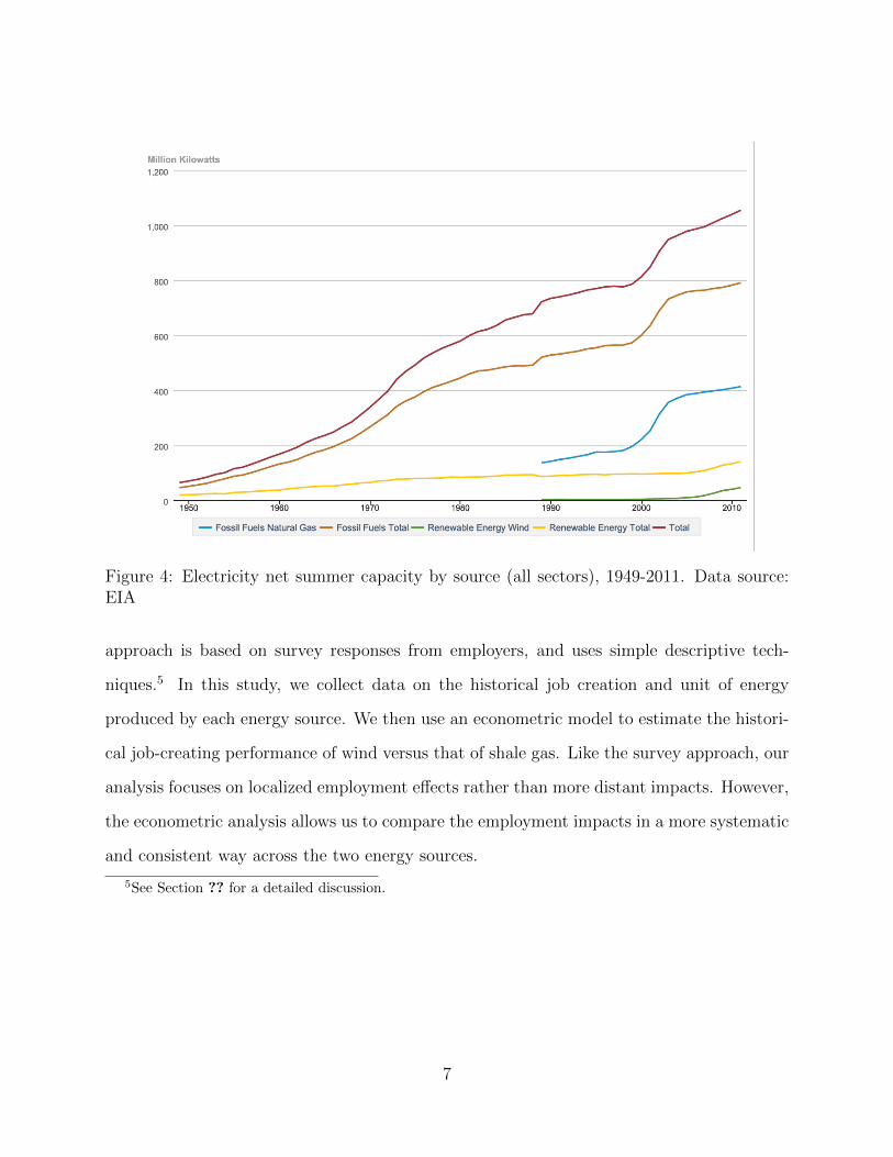
Figure 4: Electricity net summer capacity by source (all sectors), 1949-2011. Data source:EIA
approach is based on survey responses from employers, and uses simple descriptive tech-
niques.5 In this study, we collect data on the historical job creation and unit of energy
produced by each energy source. We then use an econometric model to estimate the histori-
cal job-creating performance of wind versus that of shale gas. Like the survey approach, our
analysis focuses on localized employment effects rather than more distant impacts. However,
the econometric analysis allows us to compare the employment impacts in a more systematic
and consistent way across the two energy sources.
5See Section ?? for a detailed discussion.
7
2 Literature Review
In the last few years, a large number of reports have emerged studying employment in
the shale and wind industries. While non-government organizations and consulting firms
conducted most of these studies, a few peer-reviewed journal articles have also been published
on this topic.
The I/O model focuses on the use of various inputs to production and how the goods
and services produced are allocated between various industrial sectors and consumers. I/O
models attempt to account for the economy as a whole. They capture employment multiplier
effects, as well as the macroeconomic impacts of shifts between sectors. Hence they could
account for losses in one sector (e.g., conventional oil industry) created by the growth in
another sector (e.g., wind energy). One drawback is that collecting data for an I/O model is
highly labor-intensive. As a result, the calibration process for default multiplier parameters
can be biased due to lack of information.
Two widely used I/O studies of the oil and gas industry are the IMPLAN model (see ?,
?, ?, and ?) and the RIMS II model, used by the U.S. Bureau of Economic Analysis (BEA)
(see ?).6 These studies typically find significant positive effects from the shale oil and gas
sectors on jobs, income, and economic growth.
A study of the Eagle Ford Shale (?) estimates that in 2011 shale activity raised output in
the local (14-county) region by just under $20 billion dollars and supported 38,000 full-time
jobs. If the region is extended to 20 counties, the study finds that 47,097 full-time jobs were
supported. A nationwide shale industry report (?) has found that the shale gas industry
supported 600,000 jobs in 2010. This is projected to grow to nearly 870,000 in 2015, and
to over 1.6 million by 2035. Two reports on the Marcellus shale by Pennsylvania State
6The IMPLAN model uses a national input-output dollar-flow table called the Social Accounting Matrix(SAM) to model the way a dollar injected into one sector is spent and re-spent in other sectors of theeconomy. RIMS II provides I/O multipliers that measure the effects on output, employment, and earningsfrom any changes in a region’s industrial activity.
8
University (?) and by West Virginia University (?) show that the oil and gas industry in
Pennsylvania generated $3.8 billion in value added, and over 48,000 jobs in 2009. In West
Virginia, the economic impact of the oil and natural gas industry in 2009 was estimated to
be $3.1 billion in total value added, while approximately 24,400 jobs were created.
The Jobs and Economic Development Impact (JEDI) model developed by the National
Renewable Energy Laboratory (NREL) is a series of spreadsheet-based I/O models that
estimate the economic impacts of constructing and operating power plants, fuel production
facilities, and other projects at the local (usually state) level. ? validate (or test) the
JEDI Wind Energy Model using data from NextEra’s Capricorn Ridge and Horse Hollow
facilities. They then use the model to examine the economic impact of large-scale wind-
farm construction. They found that the JEDI model overestimates local jobs during the
construction phase in smaller, rural counties, and that it underestimates by more than 50%
the number of jobs in large, urban counties. This is because the JEDI model sets the local
share of employment attributable to wind to be the same for all counties. In addition, the
JEDI model assumes 100% local share for operations and maintenance (O&M) jobs, which
might be implausible, especially in small rural counties.
An alternative approach to I/O models uses “bottom up” estimates based on indus-
try/utility surveys of project developers and equipment manufacturers, and on primary em-
ployment data from companies across manufacturing, construction, installation, and O&M.
For wind energy, most reports are analytical-based studies, and only calculate direct employ-
ment impacts. As an example, a case study on the economic effects of the Gulf wind project
in Texas reports the estimated creation of 250 - 300 jobs during the peak construction period
(9 months), and 15 - 20 permanent jobs.7
A report on the wind industry from the Natural Resources Defense Council (NRDC)
measures the number of direct jobs that a typical wind farm may create across the entire value
7Gulf Wind: Harnessing the Wind for South Texas
9
chain. They analyze each of the 14 key value-chain activities independently to determine the
number of workers involved at each step in building the wind farm. They find that a typical
wind farm of 250MW would create 1079 jobs over the lifetime of the project. Similarly, the
Renewable Energy Policy Project (REPP) has developed a spreadsheet-based model using
data based on a survey of current industry practices. They use it to calculate the number
of direct jobs from wind, solar photovoltaic, biomass, and geothermal activities that would
result from the enactment of a Renewable Portfolio Standard. They find that every 100 MW
of wind power installed creates 475 jobs in total (313 manufacturing jobs, 67 installation
jobs, and 95 jobs in O&M).
3 Data
We use data from the state of Texas. Texas has rich shale gas and oil resources and, at the
same time, it is the national leader in wind installations and a manufacturing hub for the
wind energy industry. According to EIA, Texas accounted for 40 percent of U.S. marketed
dry shale gas production in 2011, making it the leading unconventional gas producer in the
U.S. Meanwhile, Texas leads the nation in wind-powered generation capacity and it is the
first state to have reached 10,000 megawatts of wind capacity.
In Texas, there are 254 counties.8 For each county i = 1, . . . , 254, we have collected
observations for T = 132 months, or a total of 11 years (2001 - 2011), making the panel
balanced.
We use total employment in all industries as one dependent variable. We did not restrict
the data to specific industries since we want to measure total employment effects, including
indirect job-creation. This includes jobs created in upstream and infrastructure supplying
industries, as well as induced jobs, such as jobs added in sectors supplying consumer items
(food, auto, housing, etc.) and services. Another dependent variable of interest is the average
8Out of these, 77 are urban counties.
10
weekly wage since, unless the supply of labor is perfectly elastic, it should also be impacted
by an increase in the demand for workers. We use monthly employment data and quarterly
wage data from the Quarterly Census of Employment and Wages (QCEW) Database of the
Bureau of Labor Statistics (BLS).9 The latter has been adjusted to a real wage using the
implicit price GDP deflator (IPD) from BEA.10
In order to evaluate the impact from shale and wind development on employment and
on the local economy, we need to measure activity in the shale and wind industries. The
key explanatory variables we use are the number of unconventional wells completed and the
newly installed wind capacity in each county and each month, respectively.
Of course, other variables could also be used to reflect other aspects of new activity in
the shale industry. These include the number of permits issued, changes in rig counts, the
number of wells spudded, and the change in total shale gas production. We chose the number
of wells completed because the well completion date indicates the end of the construction
period for each well. We suspect that more direct and on-site jobs are created during that
period. To fully describe the impact of shale on employment, especially the multiplier effects
on job creation in the local economy, we allow well drilling activities to affect employment
with a lag, and we study both pre-completion and post-construction effects.
In the shale industry, the entire process from spudding to producing marketed output
can take up to 3-4 months. Horizontal drilling itself currently takes approximately 18-25
days from start to finish. Then wells are fractured to release the gas or oil before the well is
completed. The well is then connected to a processing facility and pipelines, which transport
the products to market. Among these activities, hydraulic fracturing and completion are the
9The QCEW employment and wage data is derived from micro data summaries of 9.1 million employerreports of employment and wages submitted by states to the BLS in 2011. These reports are based onplace of employment rather than place of residence. Average weekly wage values are calculated by dividingquarterly total wages by the average of the three monthly employment levels and then dividing the resultby 13, as there are 13 weeks in a quarter.
10The implicit price GDP deflator is the ratio of the current-dollar value of GDP to its correspondingchained-dollar value multiplied by 100.
11
●●●●●●
●●●●●
●●●●●
●
●●●
●
●
●●●●
●●●
●●●●
●
●●●●
●●
●
●
●●●●
●●●
●●●
●
●●●●
●●●
●●
●
●
●
●
●
●
●
●●
●●
●
●
●
●●
●
●
●
●
●●
●
●
●
●●●●●
●
●
●
●●
●
●
●
●●●
●
●●●
●
●●
●●
●
●●
●
●
●
●
●
●
●
●●
●
●
●
●
●
●
●
●
0 20 40 60 80 100 120
010
020
030
040
050
0
Month t
Wel
ls c
ompl
eted
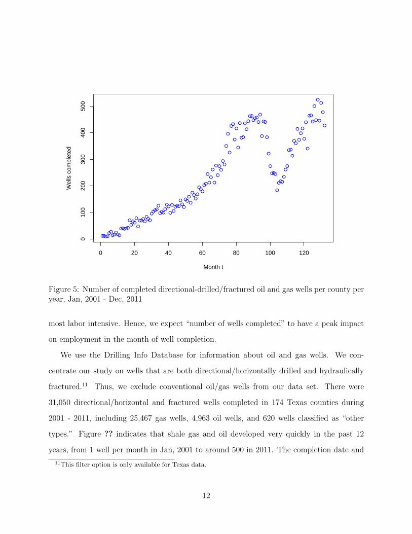
Figure 5: Number of completed directional-drilled/fractured oil and gas wells per county peryear, Jan, 2001 - Dec, 2011
most labor intensive. Hence, we expect “number of wells completed” to have a peak impact
on employment in the month of well completion.
We use the Drilling Info Database for information about oil and gas wells. We con-
centrate our study on wells that are both directional/horizontally drilled and hydraulically
fractured.11 Thus, we exclude conventional oil/gas wells from our data set. There were
31,050 directional/horizontal and fractured wells completed in 174 Texas counties during
2001 - 2011, including 25,467 gas wells, 4,963 oil wells, and 620 wells classified as “other
types.” Figure ?? indicates that shale gas and oil developed very quickly in the past 12
years, from 1 well per month in Jan, 2001 to around 500 in 2011. The completion date and
11This filter option is only available for Texas data.
12
location of each well are used to count the number of wells completed in each county each
month.
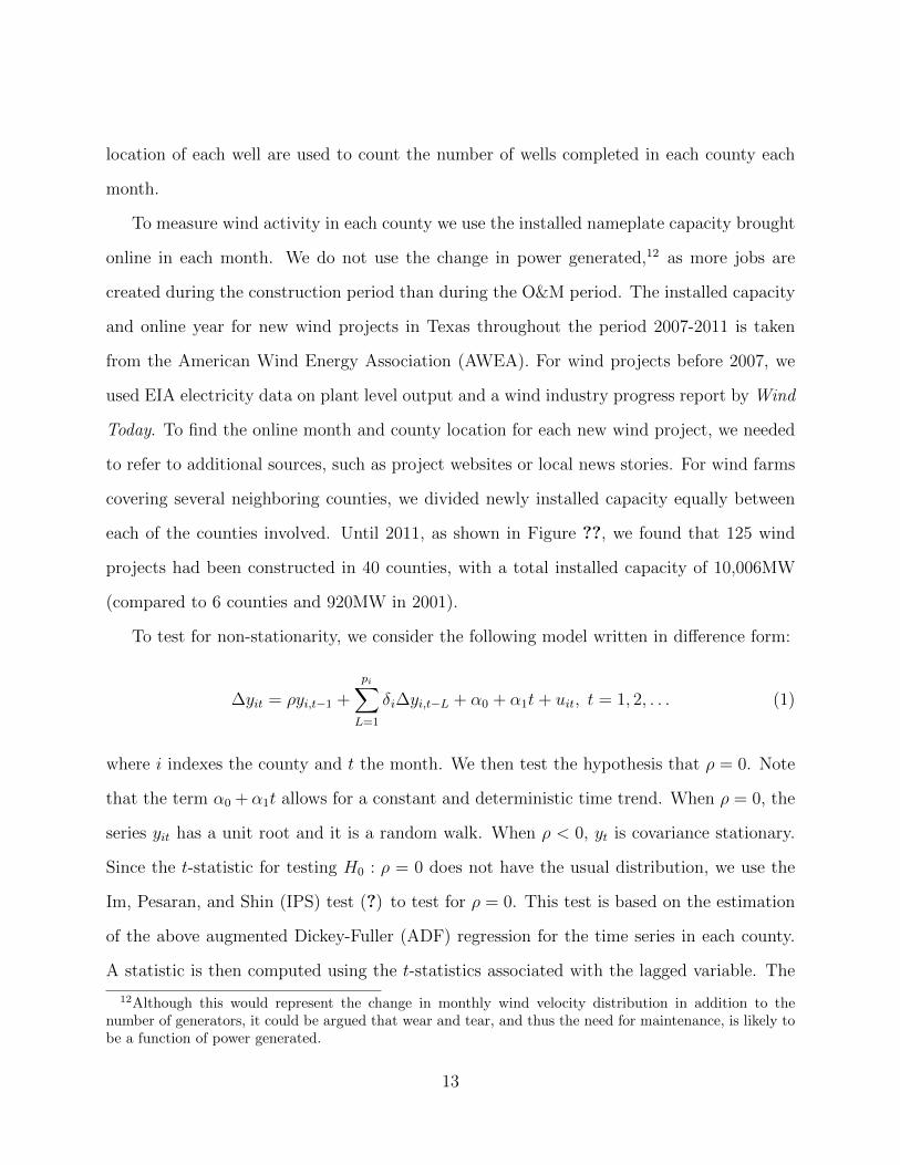
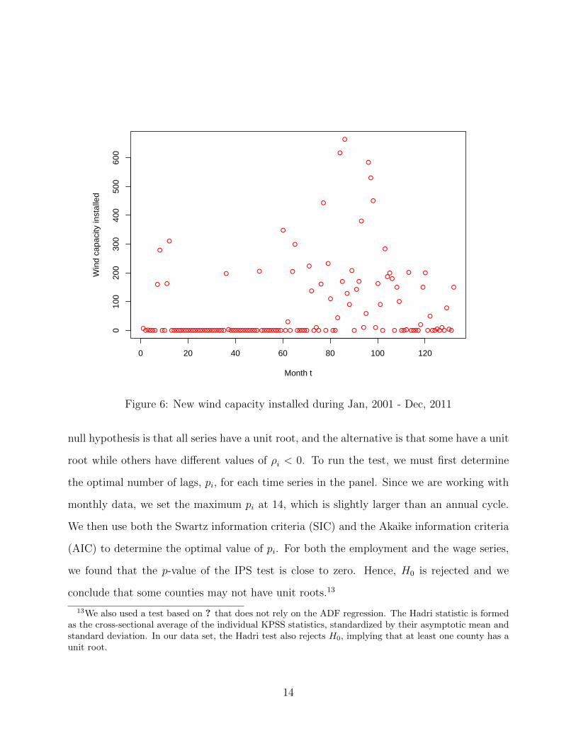
To measure wind activity in each county we use the installed nameplate capacity brought
online in each month. We do not use the change in power generated,12 as more jobs are
created during the construction period than during the O&M period. The installed capacity
and online year for new wind projects in Texas throughout the period 2007-2011 is taken
from the American Wind Energy Association (AWEA). For wind projects before 2007, we
used EIA electricity data on plant level output and a wind industry progress report by Wind
Today. To find the online month and county location for each new wind project, we needed
to refer to additional sources, such as project websites or local news stories. For wind farms
covering several neighboring counties, we divided newly installed capacity equally between
each of the counties involved. Until 2011, as shown in Figure ??, we found that 125 wind
projects had been constructed in 40 counties, with a total installed capacity of 10,006MW
(compared to 6 counties and 920MW in 2001).
To test for non-stationarity, we consider the following model written in difference form:
∆yit = ρyi,t−1 +
pi∑L=1
δi∆yi,t−L + α0 + α1t+ uit, t = 1, 2, . . . (1)
where i indexes the county and t the month. We then test the hypothesis that ρ = 0. Note
that the term α0 + α1t allows for a constant and deterministic time trend. When ρ = 0, the
series yit has a unit root and it is a random walk. When ρ < 0, yt is covariance stationary.
Since the t-statistic for testing H0 : ρ = 0 does not have the usual distribution, we use the
Im, Pesaran, and Shin (IPS) test (?) to test for ρ = 0. This test is based on the estimation
of the above augmented Dickey-Fuller (ADF) regression for the time series in each county.
A statistic is then computed using the t-statistics associated with the lagged variable. The
12Although this would represent the change in monthly wind velocity distribution in addition to thenumber of generators, it could be argued that wear and tear, and thus the need for maintenance, is likely tobe a function of power generated.
13
●●●●●●
●
●
●●
●
●
●●●●●●●●●●●●●●●●●●●●●●●
●
●●●●●●●●●●●●●
●
●●●●●●●●●
●
●
●
●
●
●
●●●●●
●
●
●●●
●
●
●
●
●
●●
●
●
●
●
●
●
●
●
●
●
●
●
●
●
●
●
●
●
●
●
●
●●●
●
●
●
●●●
●
●●●●●
●
●
●
●
●●●●●●
●
●●
●
0 20 40 60 80 100 120
010
020
030
040
050
060
0
Month t
Win
d ca
paci
ty in
stal
led
Figure 6: New wind capacity installed during Jan, 2001 - Dec, 2011
null hypothesis is that all series have a unit root, and the alternative is that some have a unit
root while others have different values of ρi < 0. To run the test, we must first determine
the optimal number of lags, pi, for each time series in the panel. Since we are working with
monthly data, we set the maximum pi at 14, which is slightly larger than an annual cycle.
We then use both the Swartz information criteria (SIC) and the Akaike information criteria
(AIC) to determine the optimal value of pi. For both the employment and the wage series,
we found that the p-value of the IPS test is close to zero. Hence, H0 is rejected and we
conclude that some counties may not have unit roots.13
13We also used a test based on ? that does not rely on the ADF regression. The Hadri statistic is formedas the cross-sectional average of the individual KPSS statistics, standardized by their asymptotic mean andstandard deviation. In our data set, the Hadri test also rejects H0, implying that at least one county has aunit root.
14
In summary, we conclude that the employment and wage series have unit roots in some
counties, while others are stationary. After applying the Dickey-Fuller Generalized Least
Squares test (DF-GLS) (at 5% level) and the KPSS test (at 10% level) to each county, we
found that in 156 counties, the DF-GLS test cannot reject a unit root, while the KPSS test
shows the presence of a unit root. In 34 counties we reject the unit root hypothesis in both
tests. In the remaining 64 counties, one test shows the presence of a unit root and the other
rejects it.
4 Econometric Issues
Working with panel data allows us to study dynamic relationships, which we cannot do using
a single cross section. It also allows us to test for the presence of specific effects in counties
with shale and wind activities versus those without. This mitigates a potential problem
with pure time series analysis, whereby many exogenous factors can change at the same
time, making it difficult to attribute an outcome to any one particular change. The panel
analysis presumes these other factors affect all counties symmetrically. In addition, a panel
data set also allows us to control for unobserved heterogeneity across counties.
4.1 Assumptions
We start with a static linear unobserved effects model:
yit = xitβ + θt + ci + uit, t = 1, 2, . . . , T, (2)
where yit is a scalar, xit is a 1×K vector for t = 1, 2, . . . , T , and β is a K × 1 vector. Here,
ci indicates a time-invariant unobservable county effect, and θt represents a series of time
fixed effects.
15
The first issue we need to address is whether the county effects ci should be taken as
fixed or random. A Hausman test yields a statistic χ2(2) = 29632 with a p-value close to zero,
indicating that the random effects approach is inconsistent. We therefore assume that the
ci are fixed.
To make the model more realistic, we allow for arbitrary dependence between the un-
observed effects, ci, and the observed explanatory variables, xit. For example, underground
geology characteristics would be included in ci, and these could be correlated with the num-
ber of wells drilled in county i. Also, wind capacity highly depends on the climate, and
especially the wind resource of the county, which is also part of the variable ci.
With a fixed effects (FE) or first difference (FD) approach, the explanatory variables are
allowed to be arbitrarily correlated with ci, but strict exogeneity conditional on ci is still
required. The assumption of strict exogeneity, introduced by ?, requires that
E(uit|xi, ci) = 0, t = 1, 2, . . . , T. (3)
That is, once xit and ci are accounted for, xis has no partial effect on yit, for s 6= t. In addition,
uit has zero mean conditional on all explanatory variables in all time periods. This is a
stronger assumption than contemporaneous exogeneity, which requires that E(uit|xit, ci) = 0.
In particular, the latter assumption says nothing about the relationship between xs and ut
for s 6= t. Sequential exogeneity, which requires that E(uit|xit,xi,t−1, . . . ,xi1, ci) = 0, for t =
1, 2, . . . , T , is stronger than contemporaneous exogeneity. It implies that xs is uncorrelated
with ut for all s ≤ t, but imposes no constraints on the correlation between xs and ut for
s > t. The pooled OLS estimator for β is consistent only if the explanatory variables satisfy
contemporaneous exogeneity and zero correlation with the unobserved individual effects.
The idea behind the fixed effects approach is to transform the equations by removing the
intertemporal mean, thereby eliminating the unobserved effects. One can then apply pooled
16
OLS to get FE estimators. Similarly, the FD approach transforms the equations by lagging
the model one period and subtracting, then applying pooled OLS to get FD estimators. As
we mentioned at the end of the previous section, we found that more than half of the counties
have highly persistent employment series. Using time series with a unit root process in a
regression equation could cause a spurious regression problem. In that case, first differencing
should be used to remove any potential unit roots.
It is standard to assume zero contemporaneous correlation; i.e., that uit is uncorrelated
with the number of wells drilled, or the wind capacity installed at t. But what about the
correlation between uit and, say, xi,t+1? Does future well drilling activity or wind-farm
construction depend on past shocks to the county’s employment? We do not believe that
such feedback is important for our study, since almost all energy produced is sold outside
the county and total employment in a county is not the main goal of energy companies.
Therefore, it seems reasonable to assume that past county employment across all industries
has a negligible effect on energy companies’ future plans.
Another issue is that a correlation might exist between uit and past xi,t−1, . . .xi,1, leading
to a failure of sequential exogeneity. This would be the case if well-drilling activity and wind
farm construction have lasting effects on local employment. One way to deal with this kind
of correlation is to include lags of the explanatory variables into the model. Strict exogeneity
may then hold if enough lags are included.14
A test of strict exogeneity is based on ?, 10.7.1.
∆yit = ∆xitβ + witγ + ∆uit, t = 2, . . . , T, (4)
In the above equation, wi,t is a subset of xi,t. Under strict exogeneity, none of the xits should
be significant explanatory variables in the first difference (FD) equation. That is, we should
find support of the hypothesis H0 : γ = 0. Carrying out this test, the F statistic on γ is
14Another remedy is to use instrumental variables, but it is often difficult to find suitable instruments.
17
0.32, with p-value 0.5695. Thus, we could not reject H0.
We have not ruled out serial correlation in the idiosyncratic error uit, that is, Corr(uit, uis) 6=
0, t 6= s. If one allows for the uits to be serially correlated over time, the usual pooled
ordinary least squares (OLS) and fixed effects (FE) standard errors are not valid, even
asymptotically. To test for the existence of serial correlation in the uits, we use the Breusch-
Godfrey/Wooldridge LM test and the Wooldridge first difference test (?). Rather than
interpreting serial correlation as a technical violation of the OLS assumption, we take it
as evidence of dynamic responses. This leads us to consider including lagged dependent
variables on the right hand side.
Observe that the strict exogeneity assumption necessarily fails in models with unobserved
effects and lagged dependent variables. The reason is that yit is correlated with uit and would
show up as part of explanatory variables at t+1, implying that E(uit|xi,t+1) 6= 0. Additional
care is required when we include lagged dependent variables as explanatory variables on the
right hand side.
4.2 The Finite Distributed Lag (FDL) Model
A finite distributed lag model is appropriate if the impact of the explanatory variables lasts
over a finite number of periods, q, and then stops. The FDL unobserved effects model
expands equation (??) to the following form:
Eit =
q∑k=0
βkwellsi,t−k +
q∑k=0
δkwcapi,t−k + ci + θt + uit (5)
where Eit denotes total employment, wellsit denotes the number of directional/fractured
wells drilled, and wcapit indicates wind capacity installed, in county i = 1, 2, . . . , 254 and
month t = 1, 2, . . . , T . Our interest lies in the pattern of coefficients {βk, δk}qk=0. The values
of β0 and δ0 capture the immediate change in Ei due to the one-unit increase in wellsi and
18

wcapi, respectively, at time t. Similarly, βk and δk capture the changes in Ei, k periods after
the new activity. At time t+ q, Ei has reverted back to its initial level, Ei,t+q = Ei,t−1.
The unit root tests in section ?? found employment and wage series have unit roots in
over half of the counties. Although we have a short panel that only covers 11 years and unit
root problems should not be a major concern, we will deal with this issue by taking first
differences of the variables in the model.
4.3 The Autoregressive Distributed Lag (ADL) Model
We are also interested in allowing for a long-lasting change in Ei in response to a change in
any of the explanatory variables.15 In principle, one could do this by allowing for a large
number of lags of the explanatory variables. In practice, however, the inclusion of many
lagged variables will reduce degrees of freedom. In addition, the fact that the resulting
explanatory variables are likely to be correlated might lead to severe multicollinearity.
The multicollinearity problem can be bypassed by including one or more lags of the
dependent variable. The model becomes an autoregressive distributed lag (ADL) model,
which is similar to the FDL model, except that the effects of the explanatory variables
persists over time at a geometrically declining rate. Denoting the number of lagged dependent
variables by p, an ADL(p, q) model with unobserved effects has the form:
Eit =
p∑j=1
λjEi,t−j +
q∑k=0
βkwellsi,t−k +
q∑k=0
δkwcapi,t−k + ci + θt + uit (6)
where {λj}pj=1 are the autoregressive coefficients. Provided that the process is stationary,
the ADL model eventually reaches a new equilibrium employment in response to a change
in wells equal to 1 that is ∑qk=0 βk
1−∑p
j=0 λj(7)
15The right lag length is rarely known in advance, or pinned down by theory.
19

higher than the original equilibrium.
Another advantage of the ADL model is that the inclusion of a lagged dependent variable
can often eliminate serial correlation, particularly if enough lags of the dependent variable are
included. Lags of the independent variables may also help eliminate serial correlation in the
error term.16 Hence, once we introduce lagged values of yit, a correct dynamic specification
implies sequential exogeneity. However, the strict exogeneity assumption is false, as we
discussed above. In this case, both the fixed effects (FE) estimator and the first difference
(FD) estimator are inconsistent.17
4.4 The Spatial Panel Model
In this section, we discuss cross-sectional dependence (XSD) in panels. This can arise, for
example, if spatial diffusion processes are present causing different panel members to be
related. In our case, shale or wind farm activity in one county could affect employment in
neighboring counties. Spatial interaction effects could be due to competition or complemen-
tarity between counties, spillovers, externalities, regional correlations in industry structures,
or shocks affecting similar industries (for example, similar weather shocks affect different
agricultural activities in both counties), as well as many other factors.
The CD and CD(p) tests (?) are used to detect XSD. These tests are based on the
averages over the time dimension of pairwise correlation coefficients for each pair of cross-
sectional units. The CD(p) test also takes into account an appropriate subset of neighboring
cross-sectional units in order to check the null of no XSD against dependence between neigh-
bors only. To do so, a spatial weights matrix, W , is needed for the CD(p) test.
16An interpretation is that the serial correlation is present in the simple model because that model ignoresthe dynamic adjustment process. Once the dynamic adjustment process is correctly specified, the serialcorrelation disappears.
17Deciding which model to use and how many lags to include is complicated by the fact that we areunlikely to have a theory to distinguish between the different models. As a result, ? and others haveadvocated starting with a general model like the ADL and testing down to a more specific model, includingthe optimal values for p and q.
20
Matrix W in our case will be a 254× 254 non-negative matrix, in which the element wij
expresses the degree of spatial proximity between the pair of objects i and j. Following ?,
the diagonal elements wii are all set to zero, to exclude self-neighbors. Furthermore, only
neighborhood effects are considered in this paper, that is, W is a contiguity matrix:18
wij =
1, if i and j are neighbors, i 6= j
0, otherwise.
(8)
In our data set, both the CD and CD(p) tests (the latter with the above W matrix) show
the presence of XSD at 0.000 level.
The contiguity matrix W is than transformed into row-standardized form, which assumes
that the impacts on a given county from all neighboring counties are equal. Given a spatial
weights matrix W , a family of related spatial econometric models can be expanded from
equation (??):
Eit = ρN∑j=1
wijEjt + β1wellsit + β2wcapit + uit, (9)
where ρ is the spatial autoregressive coefficient and N is the number of neighbors. We specify
the composite error uit following ?. They assume that spatial correlation applies to both
unobserved individual effects and the remainder error components. In this case, uit follows
a first order spatial autoregressive process of the form:
uit = λ
N∑j=1
wijujt + εit (10)
and ε follows an error component structure
εit = ci + νit (11)
18W is also called as adjacency matrix.
21
to further allow εit to be correlated over time.
5 Results
5.1 The FDL model
In this section we drop all lagged dependent variables and use the FDL approach. We
verified that the strict exogeneity assumption holds as long as enough lags of the explanatory
variables are included.
To obtain a first difference (FD) estimator, lag the model in (??) by one period and
subtract to obtain:
∆Eit =
q∑k=0
βk∆wellsi,t−k +
q∑k=0
δk∆wcapi,t−k + θ0 + θt + ∆uit, t = 2, 3, . . . , T (12)
Note that rather than dropping an overall intercept and including the differenced time dum-
mies ∆θt, we estimated an intercept and then included the time dummies θt, for T − 2 of
the remaining periods. Because the regressors involving the time dummies are non-singular
linear transformations of each other, the estimated coefficients on the other variables do not
change.
Next, we test for the presence of serial correlation in ∆uit using the Breusch-Godfrey
and Wooldridge tests for serial correlation in panels. Both tests reject H0 and show that
serial correlation remains in the idiosyncratic errors. We then increased p up to p = 36. The
results showed that serial correlation remained no matter how many lags of the explanatory
variables were included. This serial correlation may imply that the model does not fully
capture the actual dynamic adjustment process.
We proceed by computing a robust variance matrix for the FD estimator, which accom-
modates a fully general structure with respect to heteroskedasticity and serial correlation in
22
∆uit. Following ?, this robust variance matrix is consistent. To determine the appropriate
lag length, q, we posited a maintained value that should be larger than the optimal q. Here
we use q = 24. We then performed sequential F tests on the last 24 > p coefficients. We
stopped when the test rejected the H0 that the coefficients are jointly zero at a 5% level.
Using a robust variance matrix to calculate the F statistics, we drop 18 lagged explanatory
variables and assign q = 6.
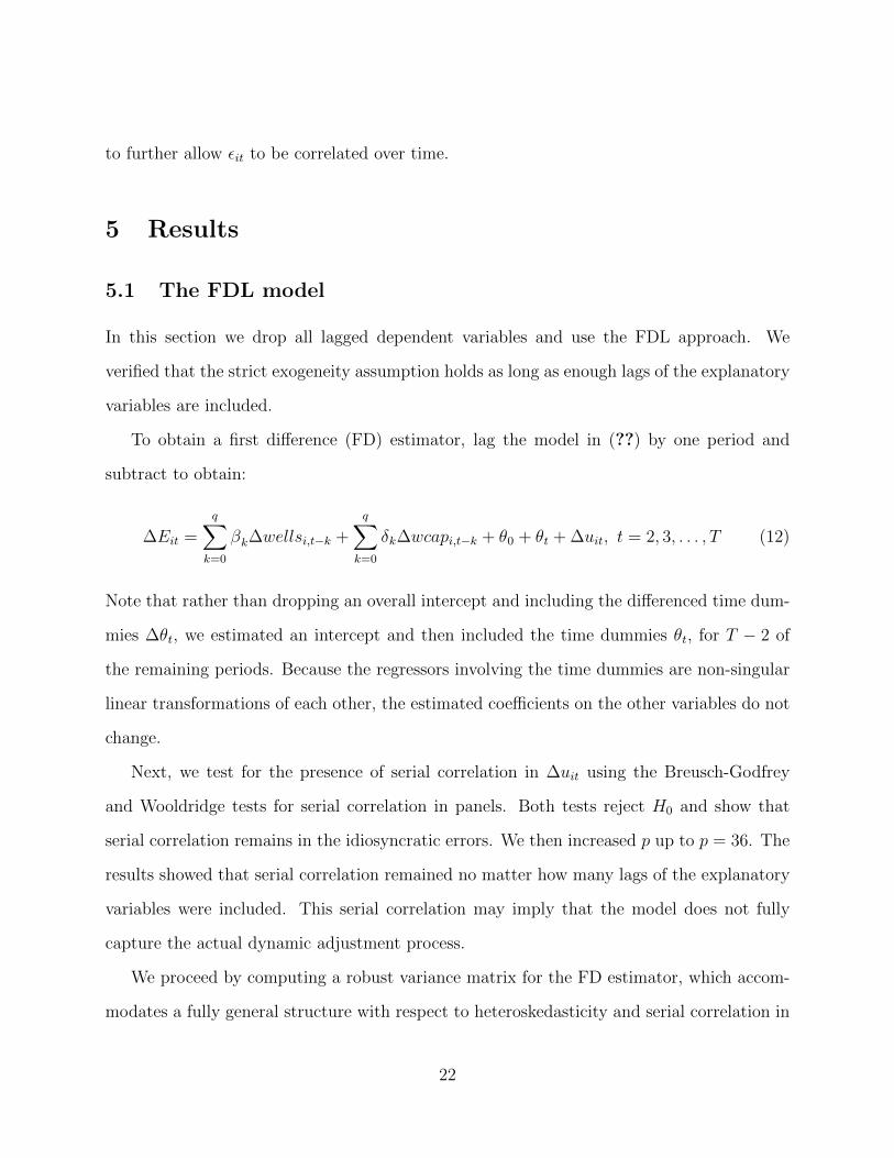
Variable Coefficient (Std. Err.) (Robust SE.)wellsit 16.31 (5.396)∗∗ [6.06]∗∗
wellsi,t−1 13.17 (6.666)∗ [7.081].
wellsi,t−2 0.932 (7.025) [2.929]wellsi,t−3 -5.519 (7.127) [6.006]wellsi,t−4 12.23 (7.119). [8.705]wellsi,t−5 17.89 (6.875)∗∗ [11.13]wellsi,t−6 22.46 (5.686)∗∗∗ [12.91].
wcapit -0.756 (1.235) [0.923]wcapi,t−1 -0.755 (1.653) [0.594]wcapi,t−2 -0.739 (1.864) [0.332]∗
wcapi,t−3 -0.212 (1.923) [0.323]wcapi,t−4 0.111 (1.865) [0.374]wcapi,t−5 0.250 (1.654) [0.432]wcapi,t−6 -0.178 (1.236) [0.266]***p < 0.001, **p < 0.01, *p < 0.05, ·p < 0.1
Table 1: FD Estimation Results, q = 6
The estimation results are reported in Table ??, with both robust standard errors and
the usual FD standard errors.19 Using robust standard errors, we find that five out of
seven coefficients of the wind installed capacity are negative and all but one are statistically
insignificantly different from zero.20 A joint F -test on H0 : δk = 0 for k = 0, 1, . . . , 6 gives
F (7, 31734) = 0.78 with p-value = 0.6001. Thus, we cannot reject the hypothesis that the
impact of wind activity on employment is not statistically significantly different from zero.
19Note that R2 = 0.00084. Since oil and gas-related employment is only 2.6% of the total employment inTexas, a low explanatory power of the regression model is perhaps to be expected.
20The order-2 lag is negative and statistically significantly different from zero at a 5% level.
23
Using robust standard errors we also find that all coefficients on the wells variables except
for the contemporaneous one are not statistically significantly different from zero at 0.05
level. The contemporaneous one is significant at the better than 0.01 level. Since substantial
correlation might exist in wells at different lags (multicollinearity), it can be difficult to
obtain precise estimates for the individual βs. However, we found wellst, wellst−1,. . . and
wellst−6 to be jointly significant: the F statistic has a p-value equal to 0.0007. Adding the
estimated coefficients of the current and lagged variables, we obtain long-term multipliers
LRPwells = 77.46. Assuming that all the jobs created are short-term (they only last for 1
month), we divide LRPwells by 12 to obtain the number of annual full-time equivalent (FTE)
jobs: 6.42.21 Given that 5482 new directional/fractured wells were drilled in Texas in 2011,
the estimates imply that about 35,000 FTE jobs would have been created.22
0 1 2 3 4 5 6
−5
05
1015
Short term impact of shale activity on employment
lag
Job
crea
ted
per
wel
l com
plet
ed
(a)
0 1 2 3 4 5 6
−0.
8−
0.6
−0.
4−
0.2
0.0
0.2
Short term impact of wind activity on employment
lag
Job
crea
ted
per
MW
win
d ca
paci
ty
(b)
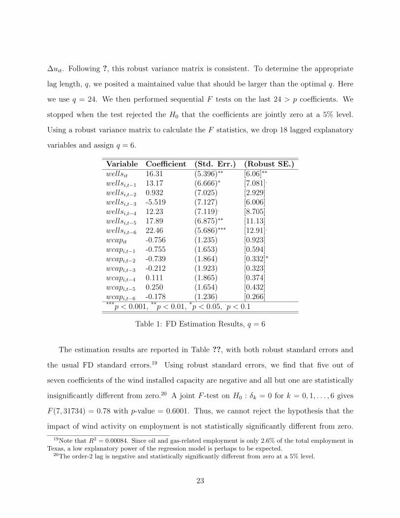
Figure 7: FD estimation results with q = 6: (a) wells (b) wind capacity
We graph the point estimates of the short-run impact of wellsk and wcapk as a function
of k in Figure ??. The lag distribution summarizes the dynamic effects on the dependent
variable of a temporary increase in the explanatory variables .
21This allows us to avoid re-counting the same person working on several different short-term jobs withina full calender year.
22The total employment in Texas in 2010 was 10, 182, 150.
24

Figure ?? shows a mainly declining trend in the impact of wells in the first three months.
This may be because workers leave after the well completion. Employment then increases
starting with month 4. This could be the result of the emergence of new business opportu-
nities in the area, resulting from the well-drilling activity. We find that the largest effect is
with the first and the last lag.
Figure ?? shows the impact from the added new wind capacity. The employment effect
is estimated to be negative at first, and then increase, peaking about five months after the
wind farm construction. However, given the estimated standard errors, we cannot establish
a relationship between wind farm construction and county employment.
5.2 The ADL model
Since the ADL model involves lagged dependent variables, the strict exogeneity assumption
is violated and both the FE and the FD estimators are inconsistent.23 To overcome this, we
use a generalized method of moments (GMM) estimator.
We again need to assign appropriate p and q to the model before we estimate it. When
we include one lagged dependent variable, Ei,t−1 (so p = 1), Wooldridge’s test for serial
correlation gives χ2(1) = 30.189, with p-value = 3.919e−8. The strong serial correlation
implies that the dynamic data generation processes has not been fully captured. When we
include one more lagged dependent variable, Ei,t−2, the test result changes to χ2(1) = 0.0081,
with p-value = 0.9285. We conclude that the error term, uit, is now serially uncorrelated.
Henceforth, we set p = 2.
As in the previous section we begin by setting q = 6. We then proceed to estimate
the two-way Arellano-Bond GMM regression. The full results are shown in Table ?? in
Appendix ??. Both the Wald and the joint F tests cannot reject that the coefficients for
23If we maintain the contemporaneous exogeneity assumption, the FE estimator’s inconsistency shrinks tozero at the rate 1/T , while the inconsistency of the FD estimator is essentially independent of T (Wooldridge,2002).
25
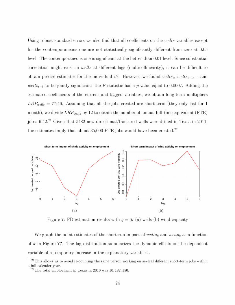
wind capacity δ0 = . . . = δ6 = 0. Thus, we again do not find any statistically significant
effect of wind farm construction on county employment. Figure ?? graphs the point estimate
of the dynamic response of employment to a unit increase in wellsit and wcapit under six
lags. It is noteworthy that these response patterns are quite similar to the ones found for the
FDL estimates and graphed in figure ??. However, due to the persistence of the impacts in
the ADL model, the long run propensity as calculated by the formula∑6
k=0 β̂k/(1− λ̂1− λ̂2)
is 3 times larger, that is, 228.93. Then the number of FTE jobs is 19.
0 1 2 3 4 5 6
−5
05
1015
Short term impact of shale activity on employment
lag
Job
crea
ted
per
wel
l com
plet
ed
(a)
0 1 2 3 4 5 6
−0.
6−
0.4
−0.
20.
0
Short term impact of wind activity on employment
lag
Job
crea
ted
per
MW
win
d ca
paci
ty
(b)
Figure 8: GMM estimation results with p = 2, q = 6: (a) wells (b) wind capacity
The estimate of the long run effect is sensitive to the values of λ̂1 and λ̂2. The sum of
the two estimated coefficients for the lagged dependent variables is 0.98. Although the test
λ1 +λ2 = 1 is rejected at the 1% level, employment might still follow a unit root process. To
address this issue, we re-estimated the same estimation using data from only the 38 counties
with stationary employment series. We obtained similar estimates: λ̂1 + λ̂2 = 0.98. We
believe that the large persistence in employment is probably due to the small explanatory
power of well drilling. Since employment in the shale gas sector is a rather small component
of total employment, most of the systematic component of employment variation would
appear in the error term. It is not surprising that this error is highly serially correlated.
26
5.3 Spatial Panel Models
Including the lagged dependent variable as a regressor in the spatial autoregression (SAR)
model introduces simultaneity bias and the OLS estimator is no longer unbiased and consis-
tent. Including the lagged dependent variable as a regressor in the spatial error model (SEM)
yields an OLS estimator that is unbiased, but inefficient. Therefore, maximum likelihood
estimation is used to estimate the parameters of both models.
Both the SAR and SEM models are estimated allowing for two-way fixed effects. The
results are reported in Table ?? in Appendix ??. We find that the spatial interaction co-
efficients of both models are statistically significantly different from zero and very similar:
ρ = 0.1730, λ = 0.1734. Also, both models show large and statistically significant coefficients
for wells, and coefficients for wcap that are not statistically significantly different from zero.
Following ?, the expectation of the dependent variable y in the SAR model y = ρWy +
Xβ + ε is
E(y) = (IN − ρW )−1Xβ (13)
Employment in county i depends on developments in neighboring counties, as a result of the
various spatial spillover effects discussed previously.
The own- and cross-partial derivatives in the SAR model take the form of an N × N
matrix that can be expressed as:
∂y/∂x′r = (IN − ρW )−1INβr (14)
These partial derivatives measure how drilling/wind activities in county j influence employ-
ment in county i. For the rth explanatory variable, the average of the main diagonal elements
of this matrix is labeled as the “direct effect.” It measures how wells drilled in a particular
county affect employment in that same county. The average of the cumulative off-diagonal
elements over all observations corresponds to the “indirect” or spillover effect. The average
27
total effect will be the sum of the two. We use equation (??) to calculate both the direct
and the indirect effects resulting from well-drilling activity.
The SAR model implies that the direct effect of well-drilling activity on employment is
225, and it is significant at the 0.000 level. The result shows that about 225 jobs would be
created per well drilled in the same county. The estimated indirect effect of well drilling ac-
tivity is 46, which increases the total effect to 271. Thus, if we only consider the direct effect,
the results would be underestimated by 17%. The result is significantly higher compared to
the FDL and even ADL estimation results (77 and 228), indicating that spatial correlation
effects are important. The FTE jobs would be 22.
Similarly, the estimated direct and indirect effects of wind activity are 0.05 and 0.01,
respectively, but neither coefficient is statistically significantly different from zero. Hence,
wind farm installation and construction was not found to have an impact on total county
employment in this data set.
5.4 Wage Effects
In this section, we examine whether there is any evidence in our data set suggesting that
shale gas and wind developments affect average weekly wages. We again employ the FD
approach. Sequential F-tests determine that q = 12. The results appear in Table ?? in
Appendix ??. The results show that the coefficients of the 4th and 9th lagged wells are sta-
tistically significantly different from zero at the 0.05 level. For wind capacity, the coefficients
of lag 1 and lag 10 are statistically significantly different from zero at the 0.05 level, while
coefficients on lags 11 and 12 are statistically significantly different from zero at the 0.01
level.
Figure ?? graphs the resulting dynamic response of wages to a unit increase in wellsit
and wcapit (12 lags). The impact from wells drilled rises and falls with a 6 month cycle.
The peaked value is about 0.3. The impact from wind capacity installation shows a quite
28
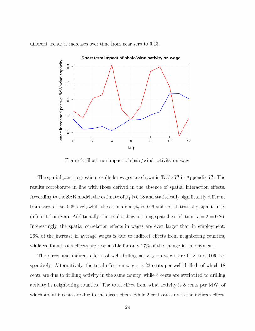
different trend: it increases over time from near zero to 0.13.
0 2 4 6 8 10 12
−0.
10.
00.
10.
20.
3
Short term impact of shale/wind activity on wage
lag
wag
e in
crea
sed
per
wel
l/MW
win
d ca
paci
ty
Figure 9: Short run impact of shale/wind activity on wage
The spatial panel regression results for wages are shown in Table ?? in Appendix ??. The
results corroborate in line with those derived in the absence of spatial interaction effects.
According to the SAR model, the estimate of β1 is 0.18 and statistically significantly different
from zero at the 0.05 level, while the estimate of β2 is 0.06 and not statistically significantly
different from zero. Additionally, the results show a strong spatial correlation: ρ = λ = 0.26.
Interestingly, the spatial correlation effects in wages are even larger than in employment:
26% of the increase in average wages is due to indirect effects from neighboring counties,
while we found such effects are responsible for only 17% of the change in employment.
The direct and indirect effects of well drilling activity on wages are 0.18 and 0.06, re-
spectively. Alternatively, the total effect on wages is 23 cents per well drilled, of which 18
cents are due to drilling activity in the same county, while 6 cents are attributed to drilling
activity in neighboring counties. The total effect from wind activity is 8 cents per MW, of
which about 6 cents are due to the direct effect, while 2 cents are due to the indirect effect.
29
6 Conclusion
We followed an econometric approach to compare job creation in wind power versus that
in the shale gas sector in Texas. We have discussed the advantages and disadvantages of a
number of different models. We then estimated them using county level data in Texas from
2001 to 2011. The results were quite consistent. Both first-difference and GMM methods
show that shale development and well-drilling activity have brought strong employment
to Texas: 77 - 271 short-term jobs or 6 - 22 FTE jobs per well. Given that 5482 new
directional/fractured wells were drilled in Texas in 2011, an estimated 35,000 - 120,000 FTE
jobs were created. In contrast, we did not find a large effect on wages. The effect on wages
corresponds to a 30-cent increase in month 4 and month 9 after each well completion.
All our estimations show that the impact from wind industry development on employ-
ment is not significantly different from zero. Its impact on wages increases gradually after
construction and peaks about one year later. We found that 13 cents are added to wages in
months 10 to 12 after construction.
While this study by no means examines all economic issues surrounding the development
of wind farms, the effects on employment in Texas counties over the period examined appear
to be insignificant. By contrast, unconventional gas production appears to be a significant
force behind employment growth in Texas counties during the same period. Further research
is needed to confirm these effects in other states and over different time periods.
30
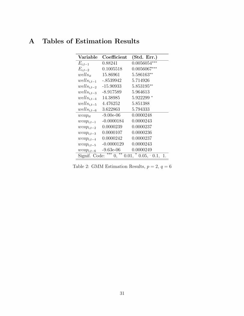
A Tables of Estimation Results
Variable Coefficient (Std. Err.)Ei,t−1 0.88241 0.0056054∗∗∗
Ei,t−2 0.1005518 0.0056067∗∗∗
wellsit 15.86961 5.586163∗∗
wellsi,t−1 -.8539942 5.714926wellsi,t−2 -15.90933 5.853195∗∗
wellsi,t−3 -8.917589 5.964613wellsi,t−4 14.38985 5.922299 ∗
wellsi,t−5 4.476252 5.851388wellsi,t−6 3.622863 5.794333wcapit -9.00e-06 0.0000248wcapi,t−1 -0.0000184 0.0000243wcapi,t−2 0.0000239 0.0000237wcapi,t−3 0.0000107 0.0000236wcapi,t−4 0.0000242 0.0000237wcapi,t−5 -0.0000129 0.0000243wcapi,t−6 -9.63e-06 0.0000249
Signif. Code: *** 0, ** 0.01, * 0.05, . 0.1, 1.
Table 2: GMM Estimation Results, p = 2, q = 6
31
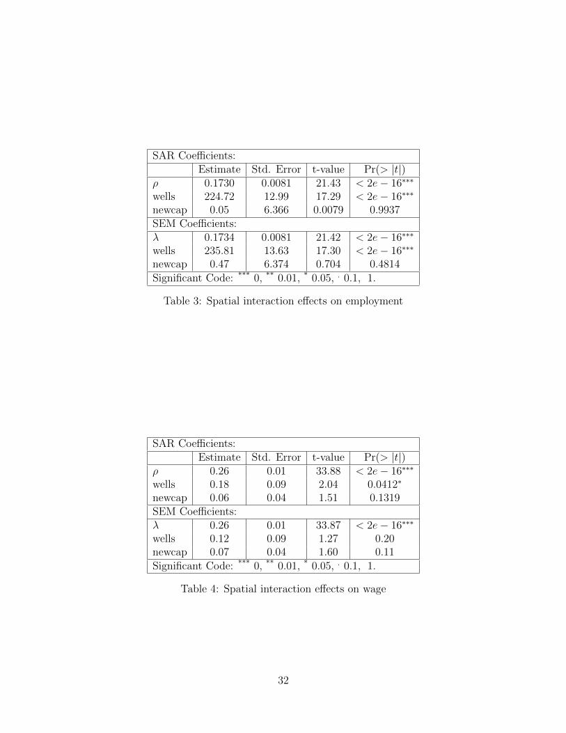
SAR Coefficients:Estimate Std. Error t-value Pr(> |t|)
ρ 0.1730 0.0081 21.43 < 2e− 16∗∗∗
wells 224.72 12.99 17.29 < 2e− 16∗∗∗
newcap 0.05 6.366 0.0079 0.9937SEM Coefficients:λ 0.1734 0.0081 21.42 < 2e− 16∗∗∗
wells 235.81 13.63 17.30 < 2e− 16∗∗∗
newcap 0.47 6.374 0.704 0.4814
Significant Code: *** 0, ** 0.01, * 0.05, . 0.1, 1.
Table 3: Spatial interaction effects on employment
SAR Coefficients:Estimate Std. Error t-value Pr(> |t|)
ρ 0.26 0.01 33.88 < 2e− 16∗∗∗
wells 0.18 0.09 2.04 0.0412∗
newcap 0.06 0.04 1.51 0.1319SEM Coefficients:λ 0.26 0.01 33.87 < 2e− 16∗∗∗
wells 0.12 0.09 1.27 0.20newcap 0.07 0.04 1.60 0.11
Significant Code: *** 0, ** 0.01, * 0.05, . 0.1, 1.
Table 4: Spatial interaction effects on wage
32
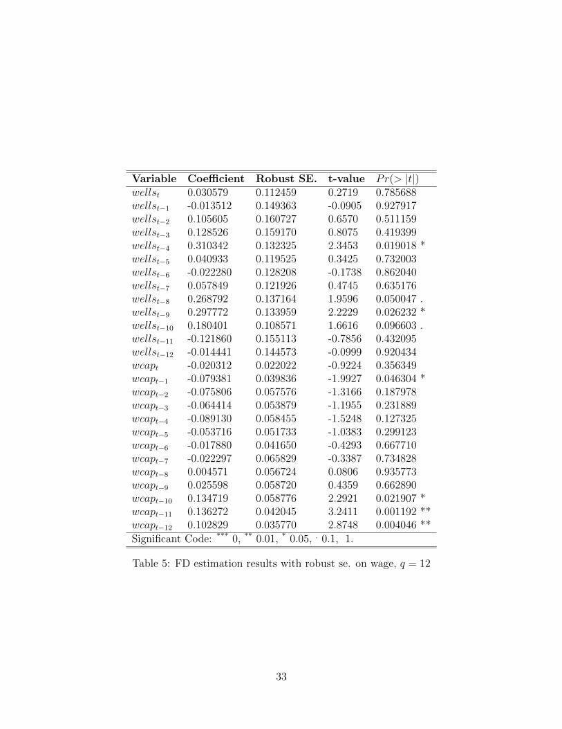
Variable Coefficient Robust SE. t-value Pr(> |t|)wellst 0.030579 0.112459 0.2719 0.785688wellst−1 -0.013512 0.149363 -0.0905 0.927917wellst−2 0.105605 0.160727 0.6570 0.511159wellst−3 0.128526 0.159170 0.8075 0.419399wellst−4 0.310342 0.132325 2.3453 0.019018 *wellst−5 0.040933 0.119525 0.3425 0.732003wellst−6 -0.022280 0.128208 -0.1738 0.862040wellst−7 0.057849 0.121926 0.4745 0.635176wellst−8 0.268792 0.137164 1.9596 0.050047 .wellst−9 0.297772 0.133959 2.2229 0.026232 *wellst−10 0.180401 0.108571 1.6616 0.096603 .wellst−11 -0.121860 0.155113 -0.7856 0.432095wellst−12 -0.014441 0.144573 -0.0999 0.920434wcapt -0.020312 0.022022 -0.9224 0.356349wcapt−1 -0.079381 0.039836 -1.9927 0.046304 *wcapt−2 -0.075806 0.057576 -1.3166 0.187978wcapt−3 -0.064414 0.053879 -1.1955 0.231889wcapt−4 -0.089130 0.058455 -1.5248 0.127325wcapt−5 -0.053716 0.051733 -1.0383 0.299123wcapt−6 -0.017880 0.041650 -0.4293 0.667710wcapt−7 -0.022297 0.065829 -0.3387 0.734828wcapt−8 0.004571 0.056724 0.0806 0.935773wcapt−9 0.025598 0.058720 0.4359 0.662890wcapt−10 0.134719 0.058776 2.2921 0.021907 *wcapt−11 0.136272 0.042045 3.2411 0.001192 **wcapt−12 0.102829 0.035770 2.8748 0.004046 **
Significant Code: *** 0, ** 0.01, * 0.05, . 0.1, 1.
Table 5: FD estimation results with robust se. on wage, q = 12
33

Editor, UWA Economics Discussion Papers: Ernst Juerg Weber Business School – Economics University of Western Australia 35 Sterling Hwy Crawley WA 6009 Australia
Email: [email protected]
The Economics Discussion Papers are available at: 1980 – 2002: http://ecompapers.biz.uwa.edu.au/paper/PDF%20of%20Discussion%20Papers/ Since 2001: http://ideas.repec.org/s/uwa/wpaper1.html Since 2004: http://www.business.uwa.edu.au/school/disciplines/economics
ECONOMICS DISCUSSION PAPERS 2012
DP NUMBER AUTHORS TITLE
12.01 Clements, K.W., Gao, G., and Simpson, T.
DISPARITIES IN INCOMES AND PRICES INTERNATIONALLY
12.02 Tyers, R. THE RISE AND ROBUSTNESS OF ECONOMIC FREEDOM IN CHINA
12.03 Golley, J. and Tyers, R. DEMOGRAPHIC DIVIDENDS, DEPENDENCIES AND ECONOMIC GROWTH IN CHINA AND INDIA
12.04 Tyers, R. LOOKING INWARD FOR GROWTH
12.05 Knight, K. and McLure, M. THE ELUSIVE ARTHUR PIGOU
12.06 McLure, M. ONE HUNDRED YEARS FROM TODAY: A. C. PIGOU’S WEALTH AND WELFARE
12.07 Khuu, A. and Weber, E.J. HOW AUSTRALIAN FARMERS DEAL WITH RISK
12.08 Chen, M. and Clements, K.W. PATTERNS IN WORLD METALS PRICES
12.09 Clements, K.W. UWA ECONOMICS HONOURS
12.10 Golley, J. and Tyers, R. CHINA’S GENDER IMBALANCE AND ITS ECONOMIC PERFORMANCE
12.11 Weber, E.J. AUSTRALIAN FISCAL POLICY IN THE AFTERMATH OF THE GLOBAL FINANCIAL CRISIS
12.12 Hartley, P.R. and Medlock III, K.B. CHANGES IN THE OPERATIONAL EFFICIENCY OF NATIONAL OIL COMPANIES
12.13 Li, L. HOW MUCH ARE RESOURCE PROJECTS WORTH? A CAPITAL MARKET PERSPECTIVE
12.14 Chen, A. and Groenewold, N. THE REGIONAL ECONOMIC EFFECTS OF A REDUCTION IN CARBON EMISSIONS AND AN EVALUATION OF OFFSETTING POLICIES IN CHINA
12.15 Collins, J., Baer, B. and Weber, E.J. SEXUAL SELECTION, CONSPICUOUS CONSUMPTION AND ECONOMIC GROWTH
34

12.16 Wu, Y. TRENDS AND PROSPECTS IN CHINA’S R&D SECTOR
12.17 Cheong, T.S. and Wu, Y. INTRA-PROVINCIAL INEQUALITY IN CHINA: AN ANALYSIS OF COUNTY-LEVEL DATA
12.18 Cheong, T.S. THE PATTERNS OF REGIONAL INEQUALITY IN CHINA
12.19 Wu, Y. ELECTRICITY MARKET INTEGRATION: GLOBAL TRENDS AND IMPLICATIONS FOR THE EAS REGION
12.20 Knight, K. EXEGESIS OF DIGITAL TEXT FROM THE HISTORY OF ECONOMIC THOUGHT: A COMPARATIVE EXPLORATORY TEST
12.21 Chatterjee, I. COSTLY REPORTING, EX-POST MONITORING, AND COMMERCIAL PIRACY: A GAME THEORETIC ANALYSIS
12.22 Pen, S.E. QUALITY-CONSTANT ILLICIT DRUG PRICES
12.23 Cheong, T.S. and Wu, Y. REGIONAL DISPARITY, TRANSITIONAL DYNAMICS AND CONVERGENCE IN CHINA
12.24 Ezzati, P. FINANCIAL MARKETS INTEGRATION OF IRAN WITHIN THE MIDDLE EAST AND WITH THE REST OF THE WORLD
12.25 Kwan, F., Wu, Y. and Zhuo, S. RE-EXAMINATION OF THE SURPLUS AGRICULTURAL LABOUR IN CHINA
12.26 Wu, Y. R&D BEHAVIOUR IN CHINESE FIRMS
12.27 Tang, S.H.K. and Yung, L.C.W. MAIDS OR MENTORS? THE EFFECTS OF LIVE-IN FOREIGN DOMESTIC WORKERS ON SCHOOL CHILDREN’S EDUCATIONAL ACHIEVEMENT IN HONG KONG
12.28 Groenewold, N. AUSTRALIA AND THE GFC: SAVED BY ASTUTE FISCAL POLICY?
35

ECONOMICS DISCUSSION PAPERS 2013
DP NUMBER AUTHORS TITLE
13.01 Chen, M., Clements, K.W. and Gao, G.
THREE FACTS ABOUT WORLD METAL PRICES
13.02 Collins, J. and Richards, O. EVOLUTION, FERTILITY AND THE AGEING POPULATION
13.03 Clements, K., Genberg, H., Harberger, A., Lothian, J., Mundell, R., Sonnenschein, H. and Tolley, G.
LARRY SJAASTAD, 1934-2012
13.04 Robitaille, M.C. and Chatterjee, I. MOTHERS-IN-LAW AND SON PREFERENCE IN INDIA
13.05 Clements, K.W. and Izan, I.H.Y. REPORT ON THE 25TH PHD CONFERENCE IN ECONOMICS AND BUSINESS
13.06 Walker, A. and Tyers, R. QUANTIFYING AUSTRALIA’S “THREE SPEED” BOOM
13.07 Yu, F. and Wu, Y. PATENT EXAMINATION AND DISGUISED PROTECTION
13.08 Yu, F. and Wu, Y. PATENT CITATIONS AND KNOWLEDGE SPILLOVERS: AN ANALYSIS OF CHINESE PATENTS REGISTER IN THE US
13.09 Chatterjee, I. and Saha, B. BARGAINING DELEGATION IN MONOPOLY
13.10 Cheong, T.S. and Wu, Y. GLOBALIZATION AND REGIONAL INEQUALITY IN CHINA
13.11 Cheong, T.S. and Wu, Y. INEQUALITY AND CRIME RATES IN CHINA
13.12 Robertson, P.E. and Ye, L. ON THE EXISTENCE OF A MIDDLE INCOME TRAP
13.13 Robertson, P.E. THE GLOBAL IMPACT OF CHINA’S GROWTH
13.14 Hanaki, N., Jacquemet, N., Luchini, S., and Zylbersztejn, A.
BOUNDED RATIONALITY AND STRATEGIC UNCERTAINTY IN A SIMPLE DOMINANCE SOLVABLE GAME
13.15 Okatch, Z., Siddique, A. and Rammohan, A.
DETERMINANTS OF INCOME INEQUALITY IN BOTSWANA
13.16 Clements, K.W. and Gao, G. A MULTI-MARKET APPROACH TO MEASURING THE CYCLE
13.17 Chatterjee, I. and Ray, R. THE ROLE OF INSTITUTIONS IN THE INCIDENCE OF CRIME AND CORRUPTION
13.18 Fu, D. and Wu, Y. EXPORT SURVIVAL PATTERN AND DETERMINANTS OF CHINESE MANUFACTURING FIRMS
13.19 Shi, X., Wu, Y. and Zhao, D. KNOWLEDGE INTENSIVE BUSINESS SERVICES AND THEIR IMPACT ON INNOVATION IN CHINA
13.20 Tyers, R., Zhang, Y. and Cheong, T.S.
CHINA’S SAVING AND GLOBAL ECONOMIC PERFORMANCE
13.21 Collins, J., Baer, B. and Weber, E.J. POPULATION, TECHNOLOGICAL PROGRESS AND THE EVOLUTION OF INNOVATIVE POTENTIAL
13.22 Hartley, P.R. THE FUTURE OF LONG-TERM LNG CONTRACTS
13.23 Tyers, R. A SIMPLE MODEL TO STUDY GLOBAL MACROECONOMIC INTERDEPENDENCE
36

13.24 McLure, M. REFLECTIONS ON THE QUANTITY THEORY: PIGOU IN 1917 AND PARETO IN 1920-21
13.25 Chen, A. and Groenewold, N. REGIONAL EFFECTS OF AN EMISSIONS-REDUCTION POLICY IN CHINA: THE IMPORTANCE OF THE GOVERNMENT FINANCING METHOD
13.26 Siddique, M.A.B. TRADE RELATIONS BETWEEN AUSTRALIA AND THAILAND: 1990 TO 2011
13.27 Li, B. and Zhang, J. GOVERNMENT DEBT IN AN INTERGENERATIONAL MODEL OF ECONOMIC GROWTH, ENDOGENOUS FERTILITY, AND ELASTIC LABOR WITH AN APPLICATION TO JAPAN
13.28 Robitaille, M. and Chatterjee, I. SEX-SELECTIVE ABORTIONS AND INFANT MORTALITY IN INDIA: THE ROLE OF PARENTS’ STATED SON PREFERENCE
13.29 Ezzati, P. ANALYSIS OF VOLATILITY SPILLOVER EFFECTS: TWO-STAGE PROCEDURE BASED ON A MODIFIED GARCH-M
13.30 Robertson, P. E. DOES A FREE MARKET ECONOMY MAKE AUSTRALIA MORE OR LESS SECURE IN A GLOBALISED WORLD?
13.31 Das, S., Ghate, C. and Robertson, P. E.
REMOTENESS AND UNBALANCED GROWTH: UNDERSTANDING DIVERGENCE ACROSS INDIAN DISTRICTS
13.32 Robertson, P.E. and Sin, A. MEASURING HARD POWER: CHINA’S ECONOMIC GROWTH AND MILITARY CAPACITY
13.33 Wu, Y. TRENDS AND PROSPECTS FOR THE RENEWABLE ENERGY SECTOR IN THE EAS REGION
13.34 Yang, S., Zhao, D., Wu, Y. and Fan, J.
REGIONAL VARIATION IN CARBON EMISSION AND ITS DRIVING FORCES IN CHINA: AN INDEX DECOMPOSITION ANALYSIS
37

ECONOMICS DISCUSSION PAPERS 2014
DP NUMBER AUTHORS TITLE
14.01 Boediono, Vice President of the Republic of Indonesia
THE CHALLENGES OF POLICY MAKING IN A YOUNG DEMOCRACY: THE CASE OF INDONESIA (52ND SHANN MEMORIAL LECTURE, 2013)
14.02 Metaxas, P.E. and Weber, E.J. AN AUSTRALIAN CONTRIBUTION TO INTERNATIONAL TRADE THEORY: THE DEPENDENT ECONOMY MODEL
14.03 Fan, J., Zhao, D., Wu, Y. and Wei, J. CARBON PRICING AND ELECTRICITY MARKET REFORMS IN CHINA
14.04 McLure, M. A.C. PIGOU’S MEMBERSHIP OF THE ‘CHAMBERLAIN-BRADBURY’ COMMITTEE. PART I: THE HISTORICAL CONTEXT
14.05 McLure, M. A.C. PIGOU’S MEMBERSHIP OF THE ‘CHAMBERLAIN-BRADBURY’ COMMITTEE. PART II: ‘TRANSITIONAL’ AND ‘ONGOING’ ISSUES
14.06 King, J.E. and McLure, M. HISTORY OF THE CONCEPT OF VALUE
14.07 Williams, A. A GLOBAL INDEX OF INFORMATION AND POLITICAL TRANSPARENCY
14.08 Knight, K. A.C. PIGOU’S THE THEORY OF UNEMPLOYMENT AND ITS CORRIGENDA: THE LETTERS OF MAURICE ALLEN, ARTHUR L. BOWLEY, RICHARD KAHN AND DENNIS ROBERTSON
14.09 Cheong, T.S. and Wu, Y. THE IMPACTS OF STRUCTURAL RANSFORMATION AND INDUSTRIAL UPGRADING ON REGIONAL INEQUALITY IN CHINA
14.10 Chowdhury, M.H., Dewan, M.N.A., Quaddus, M., Naude, M. and Siddique, A.
GENDER EQUALITY AND SUSTAINABLE DEVELOPMENT WITH A FOCUS ON THE COASTAL FISHING COMMUNITY OF BANGLADESH
14.11 Bon, J. UWA DISCUSSION PAPERS IN ECONOMICS: THE FIRST 750
14.12 Finlay, K. and Magnusson, L.M. BOOTSTRAP METHODS FOR INFERENCE WITH CLUSTER-SAMPLE IV MODELS
14.13 Chen, A. and Groenewold, N. THE EFFECTS OF MACROECONOMIC SHOCKS ON THE DISTRIBUTION OF PROVINCIAL OUTPUT IN CHINA: ESTIMATES FROM A RESTRICTED VAR MODEL
14.14 Hartley, P.R. and Medlock III, K.B. THE VALLEY OF DEATH FOR NEW ENERGY TECHNOLOGIES
14.15 Hartley, P.R., Medlock III, K.B., Temzelides, T. and Zhang, X.
LOCAL EMPLOYMENT IMPACT FROM COMPETING ENERGY SOURCES: SHALE GAS VERSUS WIND GENERATION IN TEXAS
14.16 Tyers, R. and Zhang, Y. SHORT RUN EFFECTS OF THE ECONOMIC REFORM AGENDA
14.17 Clements, K.W., Si, J. and Simpson, T. UNDERSTANDING NEW RESOURCE PROJECTS
38