Embed Size (px)
Citation preview
Submitted to Management Sciencemanuscript ()
Competing on Toxicity: The Impact of Supplier Pricesand Regulation on Manufacturers’ Substance
Replacement Strategies(Authors’ names blinded for peer review)
The recent proliferation of media reports on substances of concern has increased consumer fears, sparked scientific
debate, and highlighted the need for stronger chemical regulations. When a substance of concern is identified
(e.g., bisphenol-A (BPA) in reusable water bottles), it presents manufacturers with difficult decisions of whether
to proactively replace the substance in their products or to defer replacement and wait to see if regulation occurs.
In this paper, we examine how competition influences manufacturers’ decisions when a substance of concern is
identified within their products. We find that when manufacturers compete on toxicity, if they face a cost tradeoff
between the substance’s expected regulatory risk and the supplier price for the replacement substance, then a
high-end manufacturer can use his brand advantage to control the market. The competition between manufactur-
ers is highest when instead, the supplier charges an intermediate price for the replacement substance. To identify
ways to increase the number of manufacturers adopting a replacement, we examine whether manufacturers can
avoid competing and instead, share the cost to replace. Our results demonstrate that opportunities may exist
for manufacturers to collaborate to replace a substance, even when the shared cost to replace is greater than the
sum of their individual replacement costs.
Key words : Competition, collaboration, environmental regulations, substances of concern, game theory
1. Introduction
In recent years, the potentially-harmful chemicals contained in widely-used consumer products have
become regular topics in the mainstream media. For example, reports have been published on the poten-
tial hazards of triclosan in toothpastes (Kary 2014), bisphenol-A (BPA) in water bottles (Kuchment
2008), brominated flame retardants (BFRs) in electronics and furniture (Callahan and Roe 2012), and
phthalates in fashion goods (Pous 2012). While these substances of concern have generated consumer
fears and scientific debate, due to a lack of regulation (Fahmy 2010, Rizzuto 2013) they can still be
found in everyday consumer products. As a result, manufacturers face difficult tradeoffs when deciding
whether to replace these substances. On the one hand, replacing a substance can be very costly and it
may be unnecessary in an uncertain regulatory environment. On the other hand, due to competitive
requirements replacing a substance may be necessary and it may even present an opportunity for a
manufacturer to differentiate himself from competitors. In this study, we examine how competition
influences manufacturers’ strategic decisions when a substance of concern is identified within their
products. To identify ways to increase the number of manufacturers replacing a substance, we examine
whether manufacturers can avoid competing on toxicity and instead collaborate to replace a substance.
Our work is motivated by the efforts of market leaders in the reusable water bottle industry to replace
1
Authors’ names blinded for peer review2 Article submitted to Management Science; manuscript no. ()
bisphenol-A (BPA) from their products in 2007 – 2008 (Austen 2008, Bailin et al. 2008, Elias et al.
2013). At the time, the reusable water bottle industry was a growing market, comprised of two leading
companies, CamelBak and Nalgene. BPA, which was found in the polycarbonate plastic used to make
water bottles, was a growing substance of concern for consumers, retailers, and regulators (Kuchment
2008). Following early press coverage about the potential dangers of BPA in plastic baby bottles, envi-
ronmentally conscious customers in the reusable water bottle segment began to demand alternatives to
polycarbonate. Eastman Chemical, a supplier of copolyesters, had developed a replacement substance
called Tritan that was comparable in performance to polycarbonate plastics and did not contain BPA.
Taking into account the level of consumer sensitivity to BPA, the likelihood that the use of BPA would
be regulated, and the inherent competition to provide a BPA-free solution, CamelBak and Nalgene
had to decide whether to incur the cost to replace polycarbonate with BPA-free Tritan or to defer
replacement and wait to see if regulation would occur.
In this paper, we study a vertically differentiated market consisting of a high-end and a low-end
manufacturer selling a product that contains a substance of concern. Although the substance is not
regulated, there is a belief in the market that regulation may occur. A replacement substance is avail-
able from a supplier, but at a higher cost. The competing manufacturers must independently decide (1)
whether to proactively replace the substance or to defer replacement and wait to see if regulation hap-
pens and (2) what price to charge for their products. Many environmentalists believe that companies,
such as CamelBak and Nalgene, should never compete on toxicity. According to James Ewell, Sustain-
able Materials Director at GreenBlue, a nonprofit that focuses on making products more sustainable,
“we are trying to help companies understand that progress to solve this problem will not evolve as
rapidly if industry attempts to use toxicity as a means of differentiating their products,” (Ewell 2013).
We therefore examine ways for manufacturers to not compete on toxicity but instead work together
to replace a substance of concern. Our research adds to the growing operations management literature
that examines the negative impact competition can have on a firm’s environmental performance (e.g.,
Atasu et al. 2009, Majumder and Groenevelt 2001, Orsdemir et al. 2014, Toyasaki et al. 2010).
Our research goals are to (i) demonstrate how competition, consumer preferences, supplier prices,
and regulatory forces can facilitate or hinder manufacturers replacing a substance and (ii) identify
opportunities to increase the number of manufacturers replacing a substance of concern. Our results
show that when manufacturers compete on toxicity, if they face a cost tradeoff between the substance’s
expected regulatory risk and the supplier price for the replacement substance, then the high-end
manufacturer can use his brand advantage to control the market. For example, when the expected
regulatory risk and the supplier price are low, if the high-end manufacturer is willing to proactively
replace and sacrifice a potential cost benefit to deferring replacement, then he can charge a higher price
and capture more demand than the low-end manufacturer. The competition between the manufacturers
is highest when the supplier does not price the replacement substance in one of the extremes, but
Authors’ names blinded for peer reviewArticle submitted to Management Science; manuscript no. () 3
instead charges an intermediate price. Under these conditions, a unique asymmetric equilibrium can
occur where the low-end manufacturer proactively replaces and is a niche-provider of a higher-priced
substance-free product, and the high-end manufacturer defers replacement and captures more demand
with a lower-priced product containing the substance of concern.
When the manufacturers can share the cost to replace, opportunities may exist for them to work
together to replace a substance of concern, even when the shared cost is greater than the sum of their
individual replacement costs. For example, if the low-end manufacturer’s strategy under competition
is to defer replacement and the high-end manufacturer’s strategy is to replace, then it may be advan-
tageous for the high-end manufacturer to incur a larger portion of the shared replacement cost to
help the low-end manufacturer to replace. This is even though when the manufacturers compete, the
high-end manufacturer already charges a higher price and captures more demand than the deferring
low-end manufacturer. Helping the low-end manufacturer enables the high-end manufacturer to better
use his brand advantage to further increase both his price and demand, resulting in higher profits.
2. Literature Review
The analytical modeling of firms’ environmental investment decisions is an emerging topic within the
environmental literature (e.g., Arora and Fosfuri 2003, Bagnoli and Watts 2003, Cortazar et al. 1998,
Kraft et al. 2013a,b, Raz et al. 2013, Yalabik and Fairchild 2011). A number of these papers examine
a competition-based setting. For example, Bagnoli and Watts (2003) study the effectiveness of firms’
investments in corporate social responsibility programs in attracting environmentally sensitive con-
sumers. Yalabik and Fairchild (2011) examine the impact that competition, consumer demands, and
regulation can have on firms’ carbon abatement decisions. With respect to substances of concern, Kraft
et al. (2013a) examine a firm’s development and implementation decisions to potentially replace a
substance in a multi-period setting. The authors show how market and regulatory forces can impact
a firm’s decisions. While the foundation for our model is also firms’ replacement decisions for a sub-
stance of concern, we model a much richer competition that includes a differentiated Bertrand price
competition based on consumer preferences. Incorporating these aspects allows us to (1) examine how
the consumer utility and the supplier price can drive manufacturers’ pricing and replacement decisions
when regulations are uncertain, (2) better define the resulting market structure with respect to price
and demand, and (3) identify when manufacturers can collaborate to replace a substance of concern.
In the last decade, there has been an emerging literature that applies analytical models to examine
the impact of regulation on firms’ environmental decisions (Krysiak 2008, Maxwell and Decker 2006,
Requate 2005, Tarui and Polasky 2005). In particular, a number of works have emerged within the
operations management literature (e.g., Ata et al. 2012, Atasu et al. 2009, Drake et al. 2012, Krass
et al. 2013, Kroes et al. 2012, Plambeck and Wang 2009). The focus of these works has been on
the use and structure of financial devices (e.g., taxes, rebates, and subsidies) to incentivize firms to
Authors’ names blinded for peer review4 Article submitted to Management Science; manuscript no. ()
improve their environmental performance. Our focus is not on the design of regulation but rather
on the impact regulatory uncertainty can have on manufacturers’ decisions. Note that there exists a
stream of environmental investment literature that examines regulatory uncertainty (e.g., Baker and
Shittu 2006, Farzin and Kort 2000, Hartl 1992, Isik 2004). However, these works typically either focus
solely on policy impacts or do not consider the problem aspects that we are interested in; e.g., none
of the papers listed model competition.
Firms collaborating to solve shared business problems has been well studied in a number of differ-
ent disciplines including research and development (e.g., Bhaskaran and Krishnan 2009, D’Aspremont
and Jacquemin 1988, Jap 2001, Kamien and Tauman 1984) and supply chain management (e.g., Bak-
shi and Kleindorder 2009, Corbett and DeCroix 2001, Jacobs and Subramanian 2011, Klassen 2000,
Kurtulus et al. 2012). Within corporate sustainability, firms working together to solve environmen-
tal issues is an emerging topic with the primary focus being on collaborations between supply chain
partners such as suppliers and manufacturers (e.g., Carter and Carter 1998, Geffen and Rothenberg
2000), manufacturers and retailers (e.g., Caro et al. 2013), or both (e.g., Vachon and Klassen 2008).
Despite this, Nidumolu et al. (2014) state that “when it comes to developing collaborative solutions
to systematic [environmental] problems, very little progress has been made,” even though there is a
“growing awareness of the critical need for improved collaboration” (pp. 77-78). Too often efforts have
failed due in large part to competitive self-interests and a lack of shared purpose between collabo-
rators. We contribute to this literature a model that examines how competition can influence firms’
substance replacement decisions and that investigates opportunities for horizontal competitors (rather
than supply chain partners) to collaborate and not compete on environmental issues.
Technology adoption is one topic that has received considerable attention with regards to both firm
competition and firm collaboration. Technology adoption under competition is well-studied within
the economics literature (e.g., Fudenberg and Tirole 1985, Hannan and McDowell 1984, Hoppe 2000,
Jensen 1982, Katz and Shapiro 1986, Levin et al. 1987, Reinganum 1981) and an emerging topic within
the operations management literature (e.g., Gaimon 1989, Goyal and Netessine 2007, Huisman and
Kort 2004, Mamer and McCardle 1987, Wang and Seidmann 1995). Related to our paper, Wang and
Seidmann (1995) examine how the competition between suppliers affects their decision to adopt a
new technology (i.e., EDI). The authors find that a high adoption cost can lead to a partial adoption
equilibrium. We expand on this result in that we find a partial adoption equilibrium can occur when
a tradeoff exists between adoption cost and expected regulatory risk. Regarding the impact of market
size on technology adoption, Hannan and McDowell (1984) show that for the case of banks adopting
ATMs, firm size is positively correlated with adoption. Conversely, Levin et al. (1987) show that for the
case of grocers adopting optical scanners, firm size is negatively correlated with adoption. We show that
for the case of replacing a substance of concern, while a larger firm (i.e., higher demand firm) is more
likely to adopt a replacement than a smaller firm, he may also use his position to control the market
Authors’ names blinded for peer reviewArticle submitted to Management Science; manuscript no. () 5
by not adopting. With regards to competitors collaborating to adopt a new technology, the literature
includes papers from both the economics literature (Clemson and Knez 1988, Teece 1992, and Axelrod
1997) and the strategy literature (e.g., Hagedoorn and Schakenraad 1994, Hamel 1991, Lado et al.
1997, Shan 1990). Concerning the impact of market size on technology adoption collaboration, Shan
(1990) examine cooperative relationships between high-technology firms jointly commercializing a new
technology. They find that competitive position impacts a firm’s propensity to cooperate, and hence,
larger firms are less likely to collaborate. Conversely, Hagedoorn and Schakenraad (1994) examine
the effect of technology alliances on firm performance. They show that larger firms are more likely to
partner. Both papers are empirical in nature. We develop an analytical model to show that when a large
firm’s competitive position is limited, collaboration and helping a smaller firm to adopt a replacement
substance can actually help a large firm to better use his brand advantage to improve his profits.
3. The Model
Next, we outline the model for the competition-only scenario analyzed in §4. In §5, we adapt the model
dynamics to the cost-sharing scenario.
We consider a vertically differentiated market consisting of two types of manufacturers, a high-
end (manufacturer 1) and a low-end (manufacturer 2). The two manufacturers are differentiated by
consumer preferences for their brands. Both manufacturers sell a product that contains a substance
of concern. Although the substance of concern is not regulated, there is a belief in the market that
regulation may occur. A supplier has developed a replacement substance that is available at a per unit
wholesale price of w. The manufacturers must first decide whether to proactively replace the substance
or to defer replacement and wait to see if regulation happens. The two manufacturers compete in a
dynamic game of perfect information (i.e., they make their replacement decisions sequentially) with
the high-end manufacturer (manufacture 1) moving first. Based on manufacturer 1’s position as the
high-end provider, it is in manufacturer 1’s best interest to closely monitor the potential risks of the
substance of concern and to act first to replace the substance (if necessary). In §6, we demonstrate
that our results do not change considerably when the low-end manufacturer can replace first.
Manufacturer i’s strategy, si (i = 1, 2), is either to proactively replace the substance (R) or to defer
replacement (D). If manufacturer i replaces the substance, then in addition to the cost per unit w, he
incurs a fixed replacement cost K that represents the cost to update his supply chain to manufacture
with the new substance. We assume that the manufacturers’ replacement costs are equal. This assump-
tion keeps the model tractable and is reasonable since manufacturers’ replacement costs can be either
increasing or decreasing in demand. For example, while a manufacturer with high demand may have a
larger and more costly supply chain, he may also have more resources available to him and more influ-
ence over his suppliers. In §7, we discuss how our results change when the manufacturers’ replacement
costs are asymmetric. Note that a manufacturer’s cost to remove a substance from his product can be
Authors’ names blinded for peer review6 Article submitted to Management Science; manuscript no. ()
substantial. For example, the Consumer Electronics Association estimates that the initial compliance
requirements for the European Union’s Restriction of Hazardous Substances (RoHS) directive, which
restricts the use of only six substances, cost the global electronics industry $32 billion (Carbone 2008).
If manufacturer i defers, then he risks a possible loss in demand and potential added costs if regula-
tion occurs. However, deferring is a viable option since not all substances of concern are proven to be
harmful; e.g., aspartame in diet soft drinks (see Brody 1983 and Halliday 2008).
Once the manufacturers make their replacement decisions, they then compete in a differentiated
Bertrand competition where each manufacturer simultaneously determines the price for his product.
Manufacturer i’s demand, Di (i = 1, 2), is based on consumers’ utility function for the product and
the replacement substance. Our modeling of consumer preferences follows Moorthy (1988) and prior
literature in sustainable operations (e.g., Atasu and Souza 2013, Atasu and Subramanian 2012). The
consumers are heterogenous, with a consumer valuation of θ for manufacturer 1’s product and δθ for
manufacturer 2’s product, with θ distributed uniformly over (the normalized support) [0,1] and 0<
δ < 1. The constant δ represents the consumer valuation discount factor of manufacturer 2’s product.
In addition to their utility for the product, consumers have a fixed utility v (δv) for the replacement
substance that is only realized if manufacturer 1 (manufacturer 2) replaces. To simplify our analysis, we
normalize our market size to 1. Given prices p1 and p2, and replacement strategy (s1, s2), a consumer’s
utility is U1(θ, v) = θ+ v1s1=R− p1 for manufacturer 1’s product, and U2(θ, v) = δθ+ δv1s2=R− p2 for
manufacturer 2’s product. We define 1si∈{1,2}=R as an indicator function such that a consumer incurs
utility v (δv) from the replacement substance only if manufacturer 1 (manufacturer 2) replaces. Based
on these functions, the market is divided into high-end consumers, represented by the set {θ|U1(θ, v)≥
0,U1(θ, v)≥ U2(θ, v)}; low-end consumers, represented by the set {θ|U2(θ, v)≥ 0,U2(θ, v)> U1(θ, v)};
and consumers who do not purchase the product, represented by the set {θ|U1(θ, v) < 0,U2(θ, v) <
0}. Due to the interdependency between consumers’ utility and the manufacturers’ demands, when
solving for the manufacturers’ optimal prices, we must incorporate additional constraints based on the
consumers’ preferences (see §A.1 for a visual representation of the manufacturers’ demand problem).
We discuss and solve for the manufacturers’ demand functions in §4.
After the manufacturers make their replacement and pricing decisions, regulation of the substance
is announced with probability q. If regulation occurs and manufacturer i has not replaced, then he is
forced to replace at a cost of αK with α > 0. Parameter α can represent either a time discount (i.e.,
α < 1) or a penalty (i.e., α ≥ 1) for delaying replacement. To capture the two drivers of regulatory
risk and to simplify our notation, we define the expected regulatory risk, r= αq, such that r takes into
account both the probability of regulation occurring and the subsequent cost the manufacturer incurs.
In order to study the range of potential scenarios a manufacturer may face, we consider cases when
there is a potential benefit to delaying replacement (i.e., r < 1 and thus, rK < K) and cases when
Authors’ names blinded for peer reviewArticle submitted to Management Science; manuscript no. () 7
there is a potential risk in delaying replacement (i.e., r≥ 1 and thus, rK ≥K).1 Note that regulation
could also represent market requirements that force a manufacturer to replace. For example, many
large retailers such as Wal-Mart have banned the sale of products containing substances of concern
such as BPA and BFRs (Koch 2013, Mui 2008). To model the manufacturers’ decisions, we focus
on the demand period leading up to a potential regulation announcement, which is often very long.
For example, the length of time from the first popular press warning regarding BPA in baby bottles
until initial regulation in the U.S. was over a decade (Consumer Reports 1999, Layton 2009). Hence,
modeling the manufacturers’ decisions for only this demand period and not perpetuity is reasonable
since it captures the typical potential costs and profits a manufacturer incurs for the foreseeable future.
In summary, we present a comprehensive end-to-end model where firms’ investment decisions are
influenced by upstream supplier pricing, downstream consumer preferences, internal costs, and external
regulatory threats. The sequence of events is as follows: (i) The high-end manufacturer (manufacturer
1) decides whether to replace (R) the substance of concern or to defer replacement (D). (ii) The low-
end manufacturer (manufacturer 2) makes his replacement decision. (iii) Based on their replacement
decisions, the two manufacturers simultaneously compete in a differentiated Bertrand competition to
determine the prices for their products. (iv) Regulation occurs with probability q; if regulation occurs
and a manufacturer has not replaced the substance, then he is forced to replace. Table 1 summarizes
our notation. Our detailed theoretical analysis is given in Appendix A; results found in the appendix
are referenced A.x. To support our analysis, we conduct an extensive numerical study; the results are
referenced throughout the main text and the details of the analysis can be found in Appendix B.
4. The Manufacturers’ Competition Scenario
The manufacturers make two decisions: first, whether to proactively replace (R) the substance of
concern or to defer (D) replacement, and second, what prices to charge for their products. Following
the recursive nature of our solution method, we first discuss the manufacturers’ pricing decisions in
§4.1. Given the manufacturers’ prices, we then discuss the manufacturers’ replacement decisions in
§4.2. Our model allows us to capture the key drivers of the manufacturers’ decisions: supplier price w,
expected regulatory risk r, consumer utility for the replacement substance v, and consumer valuation
discount factor of manufacturer 2’s product δ. Note that δ represents a measure of market structure
and the heterogeneity between the manufacturers.
We define manufacturer i’s profit as:
πi(pi, p−i, (s1, s2)) =
(pi−w)Di(pi, p−i, (s1, s2))−K if si =R,
piDi(pi, p−i, (s1, s2))− rK if si =D.(1)
1 Due to delays in regulation (Grady 2010, Tavernise 2012), a manufacturer may be able to defer expensive investmentsand realize a time-discounted cost savings. Conversely, by not proactively replacing, a manufacturer may risk incurringadditional costs if regulation occurs and he is not prepared. As Mark Newton, Dell’s senior manager for environmentalsustainability, noted, “Being ahead of the curve on regulation indicates overall good management. Late adaptation hascost implications, for example the cost of making major changes in a very limited time frame” (ChemSec 2009).
Authors’ names blinded for peer review8 Article submitted to Management Science; manuscript no. ()
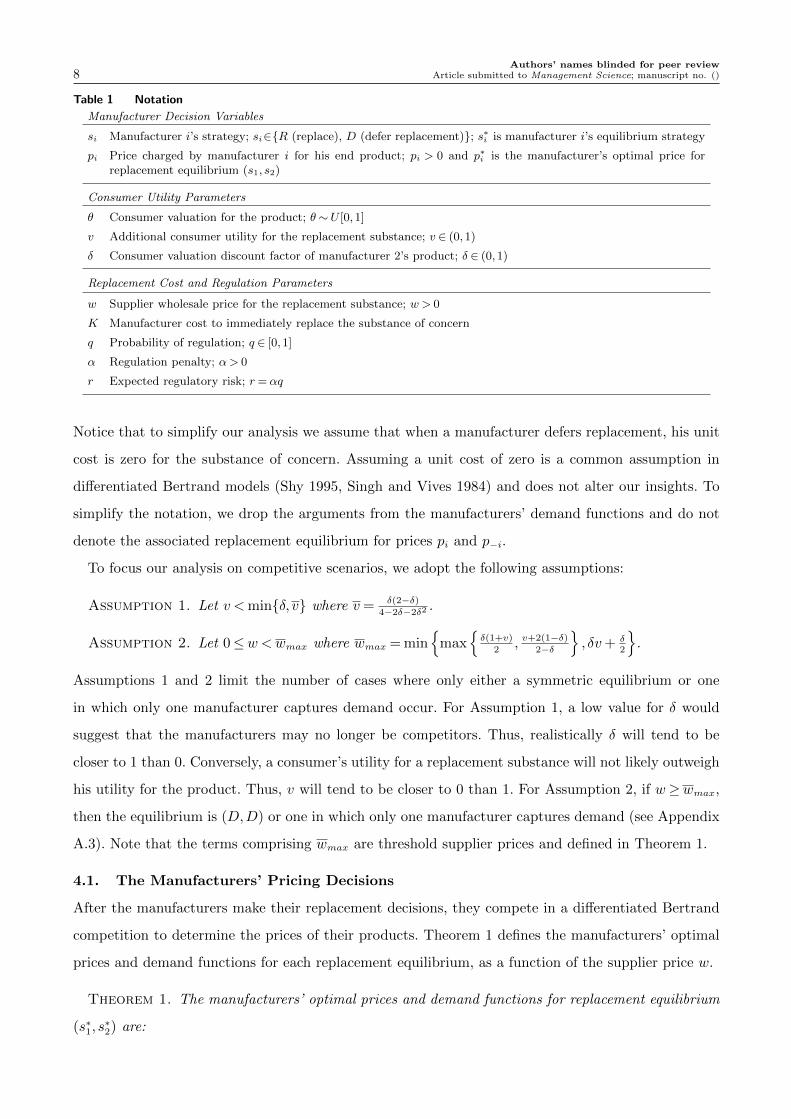
Table 1 Notation
Manufacturer Decision Variables
si Manufacturer i’s strategy; si∈{R (replace), D (defer replacement)}; s∗i is manufacturer i’s equilibrium strategy
pi Price charged by manufacturer i for his end product; pi > 0 and p∗i is the manufacturer’s optimal price forreplacement equilibrium (s1, s2)
Consumer Utility Parameters
θ Consumer valuation for the product; θ∼U [0,1]
v Additional consumer utility for the replacement substance; v ∈ (0,1)
δ Consumer valuation discount factor of manufacturer 2’s product; δ ∈ (0,1)
Replacement Cost and Regulation Parameters
w Supplier wholesale price for the replacement substance; w> 0
K Manufacturer cost to immediately replace the substance of concern
q Probability of regulation; q ∈ [0,1]
α Regulation penalty; α> 0
r Expected regulatory risk; r= αq
Notice that to simplify our analysis we assume that when a manufacturer defers replacement, his unit
cost is zero for the substance of concern. Assuming a unit cost of zero is a common assumption in
differentiated Bertrand models (Shy 1995, Singh and Vives 1984) and does not alter our insights. To
simplify the notation, we drop the arguments from the manufacturers’ demand functions and do not
denote the associated replacement equilibrium for prices pi and p−i.
To focus our analysis on competitive scenarios, we adopt the following assumptions:
Assumption 1. Let v <min{δ, v} where v= δ(2−δ)4−2δ−2δ2 .
Assumption 2. Let 0≤w<wmax where wmax = min{
max{δ(1+v)
2, v+2(1−δ)
2−δ
}, δv+ δ
2
}.
Assumptions 1 and 2 limit the number of cases where only either a symmetric equilibrium or one
in which only one manufacturer captures demand occur. For Assumption 1, a low value for δ would
suggest that the manufacturers may no longer be competitors. Thus, realistically δ will tend to be
closer to 1 than 0. Conversely, a consumer’s utility for a replacement substance will not likely outweigh
his utility for the product. Thus, v will tend to be closer to 0 than 1. For Assumption 2, if w≥wmax,
then the equilibrium is (D,D) or one in which only one manufacturer captures demand (see Appendix
A.3). Note that the terms comprising wmax are threshold supplier prices and defined in Theorem 1.
4.1. The Manufacturers’ Pricing Decisions
After the manufacturers make their replacement decisions, they compete in a differentiated Bertrand
competition to determine the prices of their products. Theorem 1 defines the manufacturers’ optimal
prices and demand functions for each replacement equilibrium, as a function of the supplier price w.
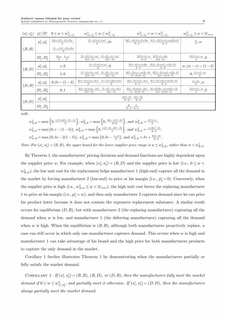
Theorem 1. The manufacturers’ optimal prices and demand functions for replacement equilibrium
(s∗1, s∗2) are:
Authors’ names blinded for peer reviewArticle submitted to Management Science; manuscript no. () 9
(s∗1, s∗2) p∗i /D
∗i 0≤w<w1
s∗1 ,s∗2
w1s∗1 ,s
∗2≤w≤w2
s∗1 ,s∗2
w2s∗1 ,s
∗2<w<w3
s∗1 ,s∗2
w3s∗1 ,s
∗2≤w<wmax
(R,R)
p∗1, p∗2
(2+v)(1−δ)+3w
3, (1−δ)+(v+w)
2, δv 2(1−δ)(1+v)+3w
4−δ , δ(1−δ)(1+v)+w(2+δ)
4−δwδ,w
(1−v)(1−δ)+3w
3
D∗1,D∗2
2+v3, 1−v
3
(1−δ)+(v−w)
2(1−δ) , (1−δ)−(v−w)
2(1−δ)2(1+v)−w
4−δ , δ(1+v)−2wδ(4−δ)
δ(1+v)−wδ
,0
(R,D)p∗1, p
∗2 v,0 (1−δ)+(v+w)
2,0 2(1−δ)+v+2w
4−δ , δ[(1−δ)+w]−v(2−δ)4−δ w, (w− v)− (1− δ)
D∗1,D∗2 1,0 (1−δ)+(v−w)
2(1−δ) , (1−δ)−(v−w)
2(1−δ)2(1−δ)+v−w(2−δ)
(1−δ)(4−δ) , δ[(1−δ)+w]−v(2−δ)δ(1−δ)(4−δ) 0, (1+v)−w
δ
(D,R)p∗1, p
∗2 0, δv− (1− δ) 2(1−δ)+(w−δv)
3, (1−δ)+(2w+δv)
3
2(1−δ)+(w−δv)4−δ , δ(1−δ)+2w+δv(2−δ)
4−δw−δvδ,w
D∗1,D∗2 0,1 2(1−δ)+(w−δv)
3(1−δ) , (1−δ)−(w−δv)3(1−δ)
2(1−δ)+(w−δv)(1−δ)(4−δ) , (2−δ)(δv−w)+δ(1−δ)
δ(1−δ)(4−δ)δ(1+v)−w
δ,0
(D,D)p∗1, p
∗2
2(1−δ)4−δ , δ(1−δ)
4−δ
D∗1,D∗2
24−δ ,
14−δ
with
w1R,R = max
{0, v(1+2δ)−(1−δ)
3
}, w2
R,R = max{
0, 3δv−δ(1−δ)2+δ
}, and w3
R,R = δ(1+v)
2;
w1R,D = max{0, v− (1− δ)}, w2
R,D = max{
0, v(2−δ)−δ(1−δ)δ
}, and w3
R,D = v+2(1−δ)2−δ ;
w1D,R = max{0, δv− 2(1− δ)}, w2
D,R = max{
0, δv− 1−δ2
}, and w3
D,R = δv+ δ(1−δ)2−δ .
Note: For (s∗1, s∗2) = (R,R), the upper bound for the lower supplier price range is w≤w1
R,R, rather than w<w1R,R.
By Theorem 1, the manufacturers’ pricing decisions and demand functions are highly dependent upon
the supplier price w. For example, when (s∗1, s∗2) = (R,D) and the supplier price is low (i.e., 0≤ w <
w1R,D), the low unit cost for the replacement helps manufacturer 1 (high-end) capture all the demand in
the market by forcing manufacturer 2 (low-end) to price at his margin (i.e., p∗2 = 0). Conversely, when
the supplier price is high (i.e., w3R,D ≤w<wmax), the high unit cost forces the replacing manufacturer
1 to price at his margin (i.e., p∗1 =w), and then only manufacturer 2 captures demand since he can price
his product lower because it does not contain the expensive replacement substance. A similar result
occurs for equilibrium (D,R), but with manufacturer 2 (the replacing manufacturer) capturing all the
demand when w is low, and manufacturer 1 (the deferring manufacturer) capturing all the demand
when w is high. When the equilibrium is (R,R), although both manufacturers proactively replace, a
case can still occur in which only one manufacturer captures demand. This occurs when w is high and
manufacturer 1 can take advantage of his brand and the high price for both manufacturers products
to capture the only demand in the market.
Corollary 1 further illustrates Theorem 1 by demonstrating when the manufacturers partially or
fully satisfy the market demand.
Corollary 1. If (s∗1, s∗2) = (R,R), (R,D), or (D,R), then the manufacturers fully meet the market
demand if 0≤w≤w2s∗1,s∗2, and partially meet it otherwise. If (s∗1, s
∗2) = (D,D), then the manufacturers
always partially meet the market demand.
Authors’ names blinded for peer review10 Article submitted to Management Science; manuscript no. ()
For equilibria (R,R), (R,D), and (D,R), when the supplier price is low, the manufacturers fully
meet the market demand. When the supplier price is high, the price of the manufacturers’ products
increases and some consumers prefer not to purchase. Thus, the manufacturers only partially meet the
market demand. For equilibrium (D,D), the manufacturers always partially meet the market demand.
Next, we compare the manufacturers’ optimal prices and demand functions within each potential
replacement equilibrium.
Lemma 1. The manufacturers’ optimal prices and demand functions are such that
(a) If (s∗1, s∗2) = (R,R) or (D,D), then (i) p∗1 > p
∗2 and (ii) D∗1 >D
∗2,
(b) If (s∗1, s∗2) = (R,D), then (i) p∗1 > p
∗2 and (ii) D∗1 ≥D∗2 for 0≤w≤wR,D, D∗1 <D
∗2 otherwise,
(c) If (s∗1, s∗2) = (D,R), then
(i) p∗1 < p∗2 for 0≤w<w1
D,R, w1D,R ≤w≤w2
D,R if v1 < v, w2D,R <w<w
3D,R if v2 < v,
w3D,R ≤w<wmax if v3 < v; p∗1 ≥ p∗2 otherwise,
(ii) D∗1 ≤D∗2 for 0≤w≤wD,R, D∗1 >D∗2 otherwise,
with w2s∗1,s∗2<ws∗1,s∗2 <w
3s∗1,s∗2
and v3 < v2 < v1;
where wR,D = δ(1−δ)+2v
δ(3−δ) , wD,R = max{δv− δ(1−δ)
2,0}
, v1 = 1−δδ
, v2 = (1−δ)(5−2δ)2δ(4−δ) , and v3 = 1−δ
2δ.
Lemma 1 highlights the market structure for each potential replacement equilibrium. When the
equilibrium is symmetric (i.e., (s∗1, s∗2) = (R,R) or (D,D)), due to his brand advantage, manufacturer
1 is the market leader with both a higher priced product and higher demand. A similar result occurs
for equilibrium (R,D) when the supplier price w is low; i.e., 0 ≤ w ≤ wR,D. The low cost for the
replacement substance allows manufacturer 1 to charge a moderate price for his product containing
the replacement and thus, generate a higher demand than manufacturer 2. When w is high (i.e.,
wR,D < w < wmax), however, manufacturer 1 no longer captures more demand than manufacturer 2.
Any benefit manufacturer 1 may gain from proactively replacing is solely based on his ability to target
a smaller market that is willing to pay a higher price for a product containing the replacement. A
similar result occurs for equilibrium (D,R), but with the additional restriction that v must be sufficient
for p∗2 > p∗1 to hold. Given consumers’ lower preference for manufacturer 2’s product, there must be
some utility for the replacement substance for manufacturer 2 to be able to charge a higher price than
manufacturer 1. As we will show, understanding how the market structure changes with respect to w
for each potential equilibrium gives insight into the manufacturers’ replacement decisions and when
opportunities exist for the manufacturers to share costs.2
In §4.2 we characterize the manufacturer replacement equilibrium. To do so, we first order the
threshold supplier prices for the four potential equilibria. To delineate the manufacturers’ strategies,
we define the following parameters for a low and high supplier price.
2 Note that not all of the outcomes presented in §4.1 occur in equilibrium for the manufacturers’ replacement game. Forexample, as will be shown, equilibrium (D,R) in Lemma 1 does not occur for 0≤w≤w2
D,R or 0≤w≤wD,R.
Authors’ names blinded for peer reviewArticle submitted to Management Science; manuscript no. () 11
Definition 1. Define wL =w2R,R ≡max
{0, 3δv−δ(1−δ)
2+δ
}and wH =w3
D,R ≡ δv+ δ(1−δ)2−δ .
Based on this, we define the replacement equilibrium for low, intermediate, and high supplier price
ranges by determining (1) manufacturer 2’s best response if s∗1 = R and if s∗1 = D; and then (2)
manufacturer 1’s best response. See Appendix A.3 for the complete analysis.
4.2. The Manufacturers’ Replacement Decisions
Next, we analyze the manufacturers’ replacement decisions. As part of our analysis, we highlight the
demand outcomes for each equilibrium. By §4.1 we know that cases can occur in which a manufacturer
does not capture demand. Since realistically a manufacturer would not be willing to proactively replace
a substance if he did not capture demand, we make the following assumption.
Assumption 3. A manufacturer is forced to exit the market if his best response payoff is less than
or equal to −K.
If Assumption 3 holds, then we replace the exiting manufacturer’s strategy with a dash in the
replacement equilibrium.3 Note that Assumption 3 does not mean that a manufacturer is forced to exit
the market if his payoff is negative or if he does not capture demand. We assume that a manufacturer
is willing to incur a negative payoff to proactively replace as long as he captures some demand and
maintains a presence in the market. In addition, if he defers replacement and r < 1, then he is willing
to stay in the market to see if regulation occurs, even if he does not capture demand.
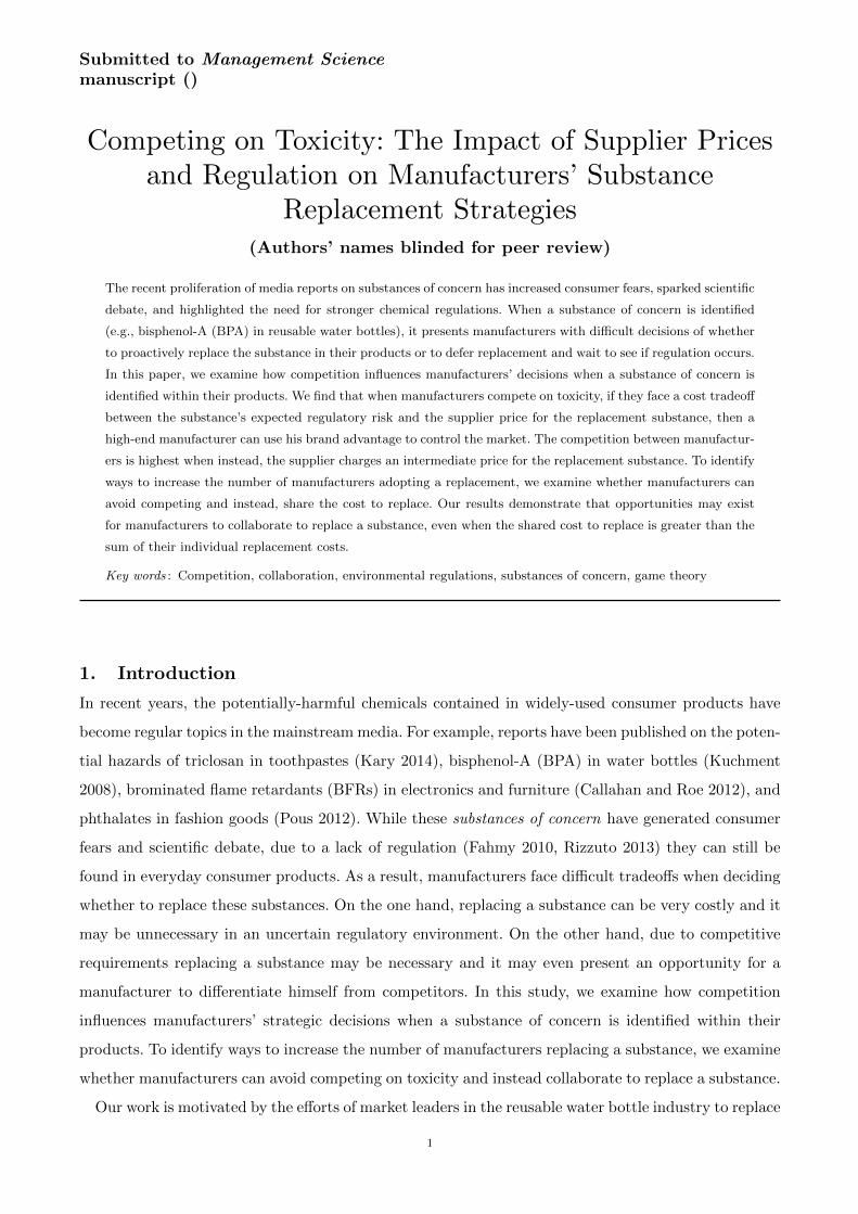
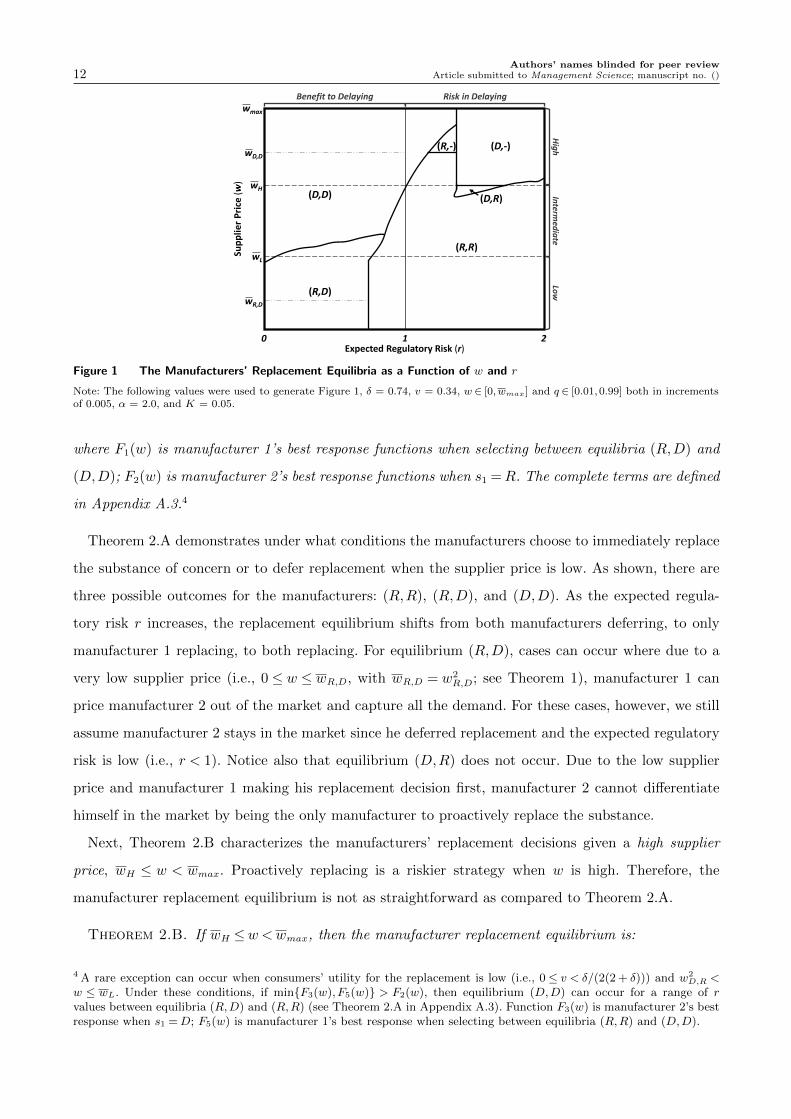
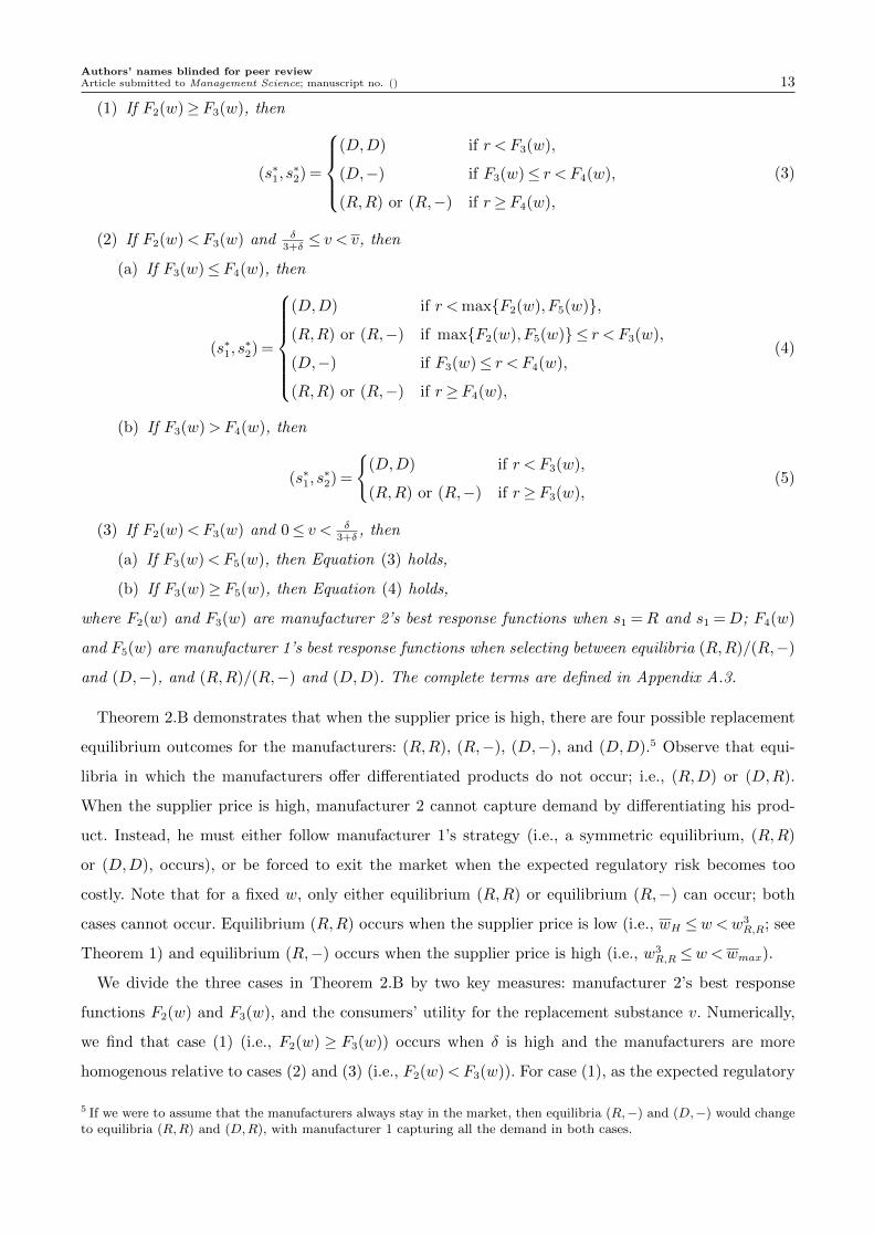
Figure 1 illustrates the manufacturers’ replacement strategies and is referenced throughout §4.2. We
define the equilibria with respect to two values: the supplier price w and the expected regulatory risk r.
This allows us to examine how a low (i.e., 0≤w≤wL), intermediate (i.e., wL <w<wH), or high (i.e.,
wH ≤w<wmax) supplier price impacts the manufacturers’ strategies when there is a potential benefit
(i.e., r < 1) or a potential risk (i.e., r≥ 1) in delaying replacement. We first discuss the manufacturers’
decisions when the supplier price is either low or high. We then discuss the more difficult to illustrate
case when the supplier price takes intermediate values.
Low and High Supplier Price: Due to the size of the manufacturer replacement equilibrium, we
divide our main result (Theorem 2) between the low and the high supplier price cases (see Appendix
A.3 for the complete theorem). Theorem 2.A characterizes the manufacturers’ replacement decisions
given a low supplier price, 0≤w≤wL.
Theorem 2.A. If 0≤w≤wL, then the manufacturer replacement equilibrium is:
(s∗1, s∗2) =
(D,D) if r < F1(w),
(R,D) if F1(w)≤ r < F2(w),
(R,R) if r≥ F2(w),
(2)
3 For these cases, we assume that the exiting manufacturer could re-enter the market. Thus, we do not solve for themonopoly prices and demands but instead continue to use the optimal prices and demand functions found in Theorem 1.
Authors’ names blinded for peer review12 Article submitted to Management Science; manuscript no. ()
Sup
plie
r P
rice
(w
)
(D,R)
Expected Regulatory Risk (r)
(R,R)
Benefit to Delaying Risk in Delaying
wH
wL
10 2
(R,-) (D,-)
(D,D)
(R,D)
wmax
Hig
hIn
termed
iate
Low
wD,D
wR,D
Figure 1 The Manufacturers’ Replacement Equilibria as a Function of w and r
Note: The following values were used to generate Figure 1, δ = 0.74, v = 0.34, w ∈ [0,wmax] and q ∈ [0.01,0.99] both in incrementsof 0.005, α = 2.0, and K = 0.05.
where F1(w) is manufacturer 1’s best response functions when selecting between equilibria (R,D) and
(D,D); F2(w) is manufacturer 2’s best response functions when s1 =R. The complete terms are defined
in Appendix A.3.4
Theorem 2.A demonstrates under what conditions the manufacturers choose to immediately replace
the substance of concern or to defer replacement when the supplier price is low. As shown, there are
three possible outcomes for the manufacturers: (R,R), (R,D), and (D,D). As the expected regula-
tory risk r increases, the replacement equilibrium shifts from both manufacturers deferring, to only
manufacturer 1 replacing, to both replacing. For equilibrium (R,D), cases can occur where due to a
very low supplier price (i.e., 0 ≤ w ≤ wR,D, with wR,D = w2R,D; see Theorem 1), manufacturer 1 can
price manufacturer 2 out of the market and capture all the demand. For these cases, however, we still
assume manufacturer 2 stays in the market since he deferred replacement and the expected regulatory
risk is low (i.e., r < 1). Notice also that equilibrium (D,R) does not occur. Due to the low supplier
price and manufacturer 1 making his replacement decision first, manufacturer 2 cannot differentiate
himself in the market by being the only manufacturer to proactively replace the substance.
Next, Theorem 2.B characterizes the manufacturers’ replacement decisions given a high supplier
price, wH ≤ w < wmax. Proactively replacing is a riskier strategy when w is high. Therefore, the
manufacturer replacement equilibrium is not as straightforward as compared to Theorem 2.A.
Theorem 2.B. If wH ≤w<wmax, then the manufacturer replacement equilibrium is:
4 A rare exception can occur when consumers’ utility for the replacement is low (i.e., 0≤ v < δ/(2(2 + δ))) and w2D,R <
w ≤ wL. Under these conditions, if min{F3(w), F5(w)} > F2(w), then equilibrium (D,D) can occur for a range of rvalues between equilibria (R,D) and (R,R) (see Theorem 2.A in Appendix A.3). Function F3(w) is manufacturer 2’s bestresponse when s1 =D; F5(w) is manufacturer 1’s best response when selecting between equilibria (R,R) and (D,D).
Authors’ names blinded for peer reviewArticle submitted to Management Science; manuscript no. () 13
(1) If F2(w)≥ F3(w), then
(s∗1, s∗2) =
(D,D) if r < F3(w),
(D,−) if F3(w)≤ r < F4(w),
(R,R) or (R,−) if r≥ F4(w),
(3)
(2) If F2(w)<F3(w) and δ3+δ≤ v < v, then
(a) If F3(w)≤ F4(w), then
(s∗1, s∗2) =
(D,D) if r <max{F2(w),F5(w)},
(R,R) or (R,−) if max{F2(w),F5(w)} ≤ r < F3(w),
(D,−) if F3(w)≤ r < F4(w),
(R,R) or (R,−) if r≥ F4(w),
(4)
(b) If F3(w)>F4(w), then
(s∗1, s∗2) =
{(D,D) if r < F3(w),
(R,R) or (R,−) if r≥ F3(w),(5)
(3) If F2(w)<F3(w) and 0≤ v < δ3+δ
, then
(a) If F3(w)<F5(w), then Equation (3) holds,
(b) If F3(w)≥ F5(w), then Equation (4) holds,
where F2(w) and F3(w) are manufacturer 2’s best response functions when s1 =R and s1 =D; F4(w)
and F5(w) are manufacturer 1’s best response functions when selecting between equilibria (R,R)/(R,−)
and (D,−), and (R,R)/(R,−) and (D,D). The complete terms are defined in Appendix A.3.
Theorem 2.B demonstrates that when the supplier price is high, there are four possible replacement
equilibrium outcomes for the manufacturers: (R,R), (R,−), (D,−), and (D,D).5 Observe that equi-
libria in which the manufacturers offer differentiated products do not occur; i.e., (R,D) or (D,R).
When the supplier price is high, manufacturer 2 cannot capture demand by differentiating his prod-
uct. Instead, he must either follow manufacturer 1’s strategy (i.e., a symmetric equilibrium, (R,R)
or (D,D), occurs), or be forced to exit the market when the expected regulatory risk becomes too
costly. Note that for a fixed w, only either equilibrium (R,R) or equilibrium (R,−) can occur; both
cases cannot occur. Equilibrium (R,R) occurs when the supplier price is low (i.e., wH ≤w<w3R,R; see
Theorem 1) and equilibrium (R,−) occurs when the supplier price is high (i.e., w3R,R ≤w<wmax).
We divide the three cases in Theorem 2.B by two key measures: manufacturer 2’s best response
functions F2(w) and F3(w), and the consumers’ utility for the replacement substance v. Numerically,
we find that case (1) (i.e., F2(w) ≥ F3(w)) occurs when δ is high and the manufacturers are more
homogenous relative to cases (2) and (3) (i.e., F2(w)<F3(w)). For case (1), as the expected regulatory
5 If we were to assume that the manufacturers always stay in the market, then equilibria (R,−) and (D,−) would changeto equilibria (R,R) and (D,R), with manufacturer 1 capturing all the demand in both cases.
Authors’ names blinded for peer review14 Article submitted to Management Science; manuscript no. ()
risk r increases, the equilibrium shifts from (D,D) to (D,−) to either (R,R) if wH ≤ w < w3R,R or
(R,−) if w3R,R ≤ w < wmax (see Equation (3)). When the expected regulatory risk is low and the
supplier price is high, both manufacturers defer replacement. However, as the expected regulatory risk
increases, this along with manufacturer 1’s choice of price for his own product, can force manufacturer
2 to exit the market (i.e., equilibrium (D,−) or (R,−) occurs) as he cannot capture enough demand
by deferring replacement to offset his high expected regulatory cost (i.e., rK). Conversely, cases (2)
and (3) occur (i.e., F2(w)<F3(w)) when the manufacturers are more heterogenous, and therefore, the
consumers’ utility for the replacement v can have a greater influence on the manufacturers’ replacement
decisions. For example, a high consumer utility for the replacement v (i.e., δ3+δ≤ v < v), can simplify
the manufacturers’ decisions such that either a symmetric equilibrium occurs (i.e., (D,D) or (R,R)),
or if the supplier price is high enough, manufacturer 1 proactively replaces and forces manufacturer 2
out of the market (i.e., (R,−)); see Equation (5).
Lemma 2 highlights key insights into the occurrence of equilibria (R,R) and (R,D) when the supplier
price is low and equilibria (D,D), (D,−), and (R,−) when the supplier price is high.
Lemma 2. The manufacturer replacement equilibrium is such that:
(a) When the supplier price is low, 0≤w≤wL,
(i) If r≥ 1, then (s∗1, s∗2) = (R,R),
(ii) Only when r < 1, can (s∗1, s∗2) = (R,D) occur.
(b) When the supplier price is high, wH ≤w<wmax,
(i) If r < 1 and wD,D ≤w<wmax, then (s∗1, s∗2) = (D,D),
(ii) Only when r≥ 1, can (s∗1, s∗2) = (D,−) or (R,−) occur.
With wD,D = max{min{w3R,R,w
3R,D},wH}.
The manufacturers’ strategies are simplified when a cost tradeoff does not exist between the supplier
price and the expected regulatory risk. For example, if r≥ 1 and the supplier price is low 0≤w≤wL,
then as shown in the lower right region of Figure 1, the equilibrium is always (R,R). The expected
cost of regulation and the low unit cost for the replacement substance induce both manufacturers to
proactively replace. A similar result occurs when r < 1 and the supplier price is high wD,D ≤w<wmax(i.e., the upper left region in Figure 1), but with both manufacturers deferring to save costs.
The supplier price and the expected regulatory risk also define when an asymmetric equilibrium with
only manufacturer 1 proactively replacing occurs. When the supplier price is low, equilibrium (R,D)
can only occur when r < 1. This implies that manufacturer 1 can differentiate his product with the
replacement substance if he is willing to incur a cost to proactively replace; i.e., K > rK. The additional
cost, however, is worth manufacturer 1’s investment since by Lemma 1 he can charge a higher price
and generate more demand than manufacturer 2 when equilibrium (R,D) occurs in the low supplier
price range.6 Conversely, when the supplier price is high, equilibria (D,−) and (R,−) can only occur
6 Manufacturer 1’s demand is greater than manufacturer 2’s since wR,D >wL.
Authors’ names blinded for peer reviewArticle submitted to Management Science; manuscript no. () 15
when r ≥ 1. Under these conditions, due to the high supplier price, manufacturer 2 cannot capture
demand by proactively replacing (i.e., s2 =R). However, due to the high expected regulatory risk and
manufacturer 1’s ability to use his brand advantage to force the low-end manufacturer to charge a
low price, deferring replacement (i.e., s2 =D) is an even less profitable strategy for manufacturer 1.
Therefore, manufacturer 2’s expected profit is −K and he is forced to exit the market.
Intermediate Supplier Price: The manufacturers’ most difficult replacement decisions occur when
the supplier offers an intermediate wholesale price; i.e., wL <w<wH . By not pricing the replacement
substance in one of the extremes (high or low), the supplier forces the manufacturers to evaluate
the difficult tradeoff between incurring additional costs to proactively replace versus possibly losing
demand and incurring regulatory costs if they defer replacement. First, we demonstrate that within
the intermediate supplier price range, all four potential replacement equilibrium can occur.
Lemma 3. If wL <w <wH , then the manufacturer replacement equilibrium can be (R,R), (R,−),
(R,D), (D,R), or (D,D). Equilibrium (R,−) only occurs when w3R,R ≤w<wH and δ
2−δ ≤ v < v.
Within this price range, both manufacturers almost always incur demand (by Lemma 3, equilibrium
(R,−) only occurs when both w and v are high). It is not possible to cleanly characterize the manufac-
turer replacement equilibrium for an intermediate supplier price due to the large number of conditions
required. Instead, we numerically examine the manufacturers’ most frequently occurring strategies as
r increases (for a fixed w). By Table 2, the two most frequently occurring cases are when either the
equilibrium shifts from (D,D) to (R,R) or from (D,D) to (R,D) to (R,R) as r increases.
Table 2 Intermediate Supplier Price: Manufacturers’ Replacement Decisions
Replacement equilibrium as r increases % of Median(for a fixed w) Cases w v δ(D,D) to (R,R) 51.5% 0.20 0.24 0.69(D,D) to (R,D) to (R,R) 27.8% 0.20 0.34 0.69(D,D) to (R,R) to (D,R) to (R,R) 11.0% 0.20 0.14 0.64(D,D) to (D,R) to (R,R) 5.3% 0.15 0.04 0.74(R,D) to (R,R) 2.8% 0.25 0.39 0.69
Note: A total of 28,140 scenarios were tested, resulting in 1,407 fixed w cases. The above strategies represent 98.4% of all casestested. Expected regulatory risk r values ranged from 0 to 2.
Unlike the low and the high supplier price cases, both equilibria (R,D) and (D,R) can occur when
the supplier charges an intermediate price. Consistent with our findings from the low supplier price
case, we numerically find that equilibrium (R,D) only occurs if r < 1 and that manufacturer 1 is able
to capture more demand with a higher priced product than manufacturer 2. Conversely, equilibrium
(D,R) only occurs if r≥ 1. As shown in Table 2, when consumers’ utility for the replacement is very
low (i.e., v = 0.14 or 0.04), manufacturer 1 can benefit by ignoring his brand advantage and ability
to replace first, and letting manufacturer 2 capture demand by being the only manufacturer in the
market with a product containing the replacement.7 Interestingly, for equilibrium (D,R), manufacturer
7 A low value for v also influences the size of this price range. The width of the intermediate price range is decreasing inv (Lemma A.2), thus the supplier’s choice of price is more likely to fall in the intermediate price range when v is low.
Authors’ names blinded for peer review16 Article submitted to Management Science; manuscript no. ()
2 often competes as a niche provider with a higher-priced substance-free product, while manufacturer
1 captures more demand with a lower-priced product.
To summarize §4, we illustrate three key insights. First, the manufacturers’ decisions are simplified
when the supplier charges a low (high) price and the expected regulatory risk is high (low). For this case,
a symmetric equilibrium occurs in which both manufacturers proactively replace (defer replacement).
Second, when there exists a cost trade-off between the expected regulatory risk and the supplier price,
the high-end manufacturer can control the market. For example, when the expected regulatory risk and
the supplier price are low, if the high-end manufacturer is willing to proactively replace and sacrifice
a potential cost benefit to deferring replacement (i.e., K > rK), then he can use his brand advantage
to charge a higher price and capture more demand than the low-end manufacturer. Conversely, when
both the supplier price and the expected regulatory risk are high, the high-end manufacturer can force
the low-end manufacturer to exit the market by limiting his ability to generate a high enough profit
to offset potential regulatory costs.8 Finally, the competition between the manufacturers is the highest
when the supplier offers an intermediate price for the replacement substance. In this price range,
typically both manufacturers capture some demand. In addition, equilibria in which the manufacturers
offer differentiated products can occur, with either the high-end (i.e., (R,D)) or the low-end (i.e.,
(D,R)) manufacturer proactively replacing.
Based on our understanding of the manufacturers’ replacement and pricing decisions under com-
petition, in §5 we examine whether opportunities exist for the manufacturers to avoid replacement
competition and instead, work together to replace the substance of concern.
5. The Manufacturers’ Cost-Sharing Scenario
Next, we examine opportunities for manufacturers to not compete on toxicity but instead, collaborate
to replace a substance of concern. In many industries, firms often share suppliers and have similar
components in their products. Within these industries, opportunities may exist for competitors to work
together and share the cost to implement a replacement substance. For example, leaders within the
jewelry industry collaborated to eliminate the use of cadmium after it was identified as a substance of
concern (Associated Press 2010). Within the furniture industry, manufacturers recently collaborated to
set industry-wide sustainability standards which included stringent self-regulation regarding chemicals
of concern (BIFMA 2014). Our goal is to identify ways to increase the number of manufacturers
replacing a substance of concern and thus, decrease the number of consumers exposed to the substance.
Nidumolu et al. (2014) characterize corporate environmental collaborations in two ways: (1) whether
the focus is either outcome or process based; and (2) whether the partnership is solely corporations
or includes additional stakeholders such as nonprofits and governments. Our approach is to model an
8 Due to the high-end manufacturer’s brand advantage and his ability to move first in the replacement game, outcomesin which only the low-end manufacturer captures demand do not occur for 0≤w<wmax (see Lemma A.1).
Authors’ names blinded for peer reviewArticle submitted to Management Science; manuscript no. () 17
outcome-based model with a simplified cost-sharing scenario, where the partnership is between manu-
facturers 1 and 2 (see Appendix A.4 for the detailed analysis). To analyze this setting, we define KC as
the total shared cost for both manufacturers to replace the substance of concern, with manufacturer 1
paying tKC , manufacturer 2 paying (1− t)KC , and t∈ [0,1]. We do not restrict KC to be less than or
greater than the sum of the manufacturers’ individual replacement costs 2K. We modify the sequence
of events from Section 3 as follows: before competing to replace the substance (with manufacturer 1
acting first), the manufacturers can choose not to compete and instead, share the cost to replace. We
assume that the manufacturers share the cost to replace if a negotiated value of t∈ [0,1] can be found
such that both manufacturers have higher profits under cost sharing than under competition. To deter-
mine t, we apply a Nash bargaining solution to model the negotiation of costs, with the manufacturers’
status-quo points being their profits if they were to compete. Modeling cooperative settings through
the use of bargaining solutions is a common practice within the operations literature (e.g., Bakshi and
Kleindorder 2009, Nagarajan and Sosic 2008, Plambeck and Taylor 2005).
If the manufacturers share the cost to replace, then they both replace with manufacturer 1’s profit
equal to π1(p1, p2) = (p1 −w)D1(p1, p2)− tKC and manufacturer 2’s profit equal to π2(p2, p1) = (p2 −
w)D2(p2, p1)− (1− t)KC . Although the manufacturers work together to replace the substance, they
still compete on price with the resulting optimal prices and demand functions equal to those from the
price competition for equilibrium (R,R) (see Theorem 1). If an agreed upon value of t∈ [0,1] cannot be
negotiated, then the manufacturers compete to replace the substance. Our model setup supports Lado
et al. (1997) and Nidumolu et al. (2014), who emphasize that the most successful collaborative models
combine competitive and cooperative aspects to achieve superior performance.
We first define for each possible manufacturer replacement equilibrium under competition, the condi-
tions under which both manufacturers prefer to share the cost to replace. Recall that πi(p∗1, p∗2, (s
∗1, s∗2))
is manufacturer i’s profit under competition equilibrium (s∗1, s∗2).
Theorem 3. The manufacturers share the cost to replace
(a) If (s∗1, s∗2) = (R,R) or (R,−), and KC ≤ 2K,
(b) If (s∗1, s∗2) = (R,D), (D,R), (D,−), or (D,D), and 1 − G2(w)−π2(p∗2,p
∗1,(s∗1,s∗2))
KC≤ t∗s∗1,s∗2
≤G1(w)−π1(p∗1,p
∗2,(s∗1,s∗2))
KC,
and compete otherwise;
where Gi(w) = (p∗i −w)Di(p∗i , p∗−i) is manufacturer i’s margin times demand under cost sharing and
t∗s∗1,s∗2= max
[0,min
[1, 1
2+
[G1(w)−G2(w)]−[π1(p∗1,p∗2,(s∗1,s∗2))−π2(p
∗2,p∗1,(s∗1,s∗2))]
2KC
]]is the Nash bargaining solution
for replacement equilibrium (s∗1, s∗2).
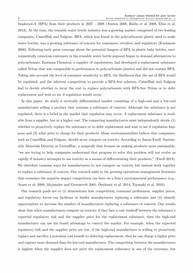
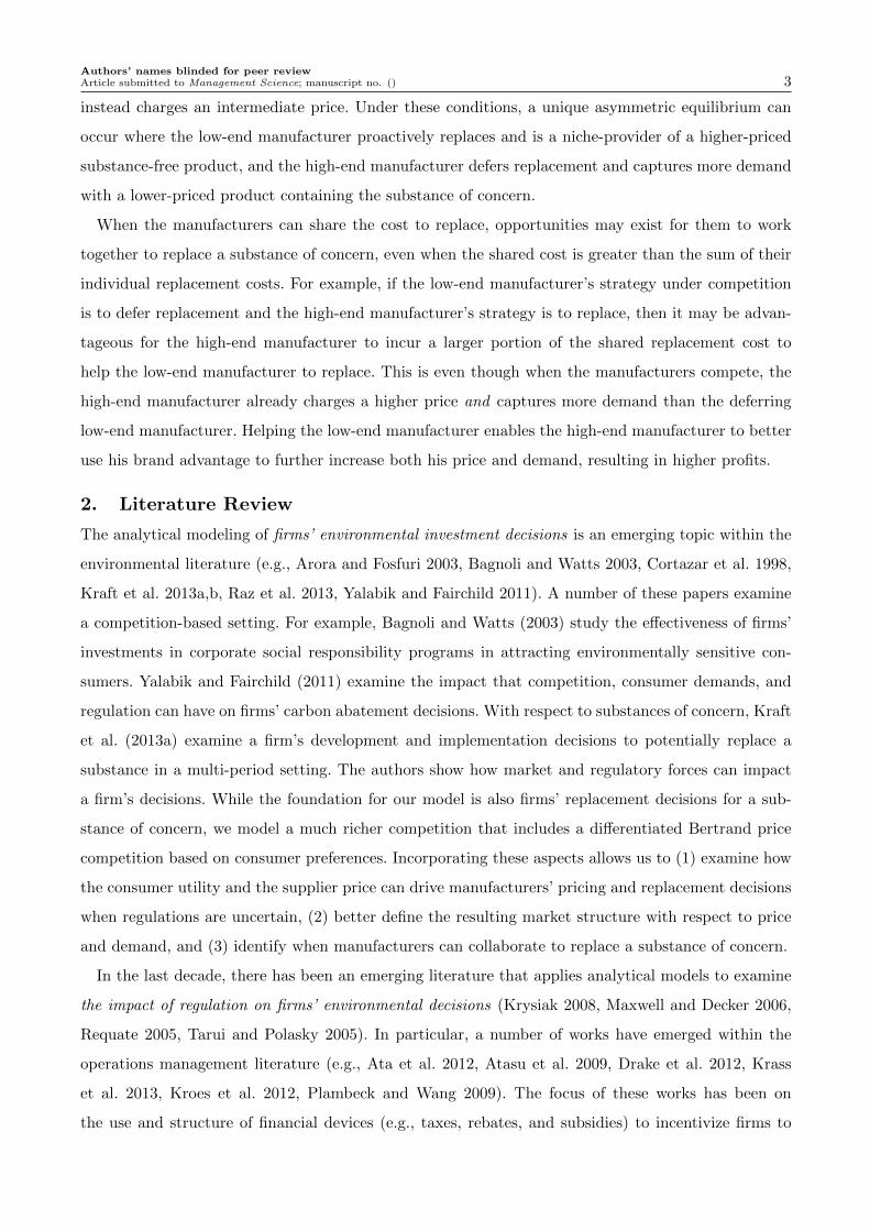
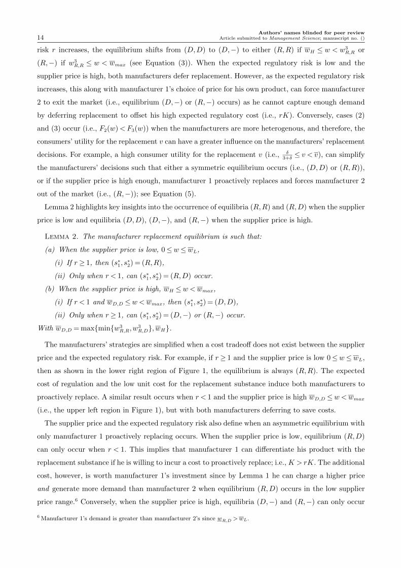
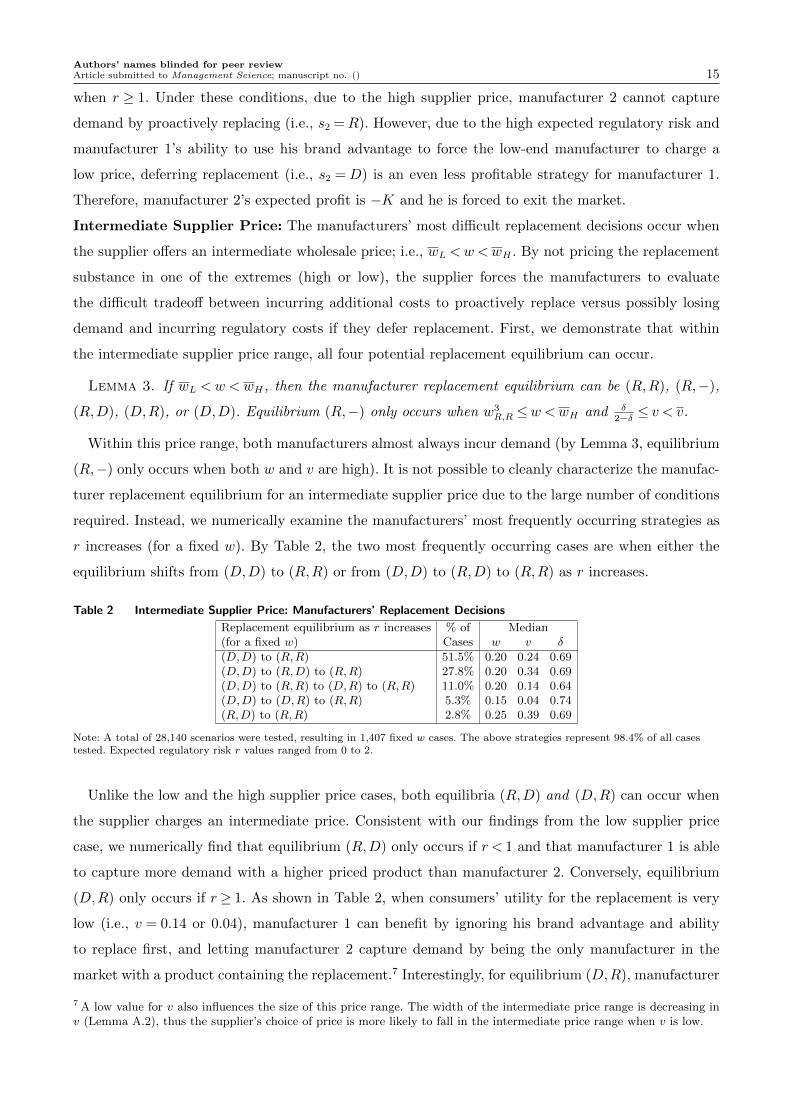
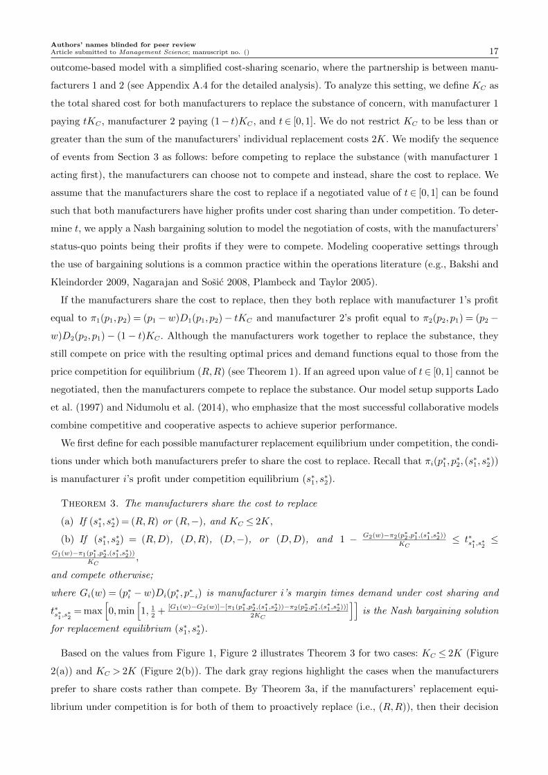
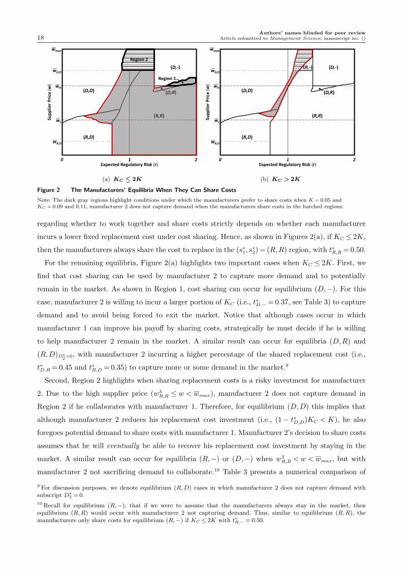
Based on the values from Figure 1, Figure 2 illustrates Theorem 3 for two cases: KC ≤ 2K (Figure
2(a)) and KC > 2K (Figure 2(b)). The dark gray regions highlight the cases when the manufacturers
prefer to share costs rather than compete. By Theorem 3a, if the manufacturers’ replacement equi-
librium under competition is for both of them to proactively replace (i.e., (R,R)), then their decision
Authors’ names blinded for peer review18 Article submitted to Management Science; manuscript no. ()
Sup
plie
r P
rice
(w
)
Expected Regulatory Risk (r)10 2
wH
wL
wmax
wD,D
(D,R)
(R,R)
(R,-) (D,-)
(D,D)
(R,D)wR,D
Region 2
Region 1
(a) KC ≤ 2K
Sup
plie
r P
rice
(w
)
Expected Regulatory Risk (r)10 2
wH
wL
wmax
wD,D
(D,R)
(R,R)
(R,-) (D,-)
(D,D)
(R,D)wR,D
(b) KC > 2K
Figure 2 The Manufacturers’ Equilibria When They Can Share Costs
Note: The dark gray regions highlight conditions under which the manufacturers prefer to share costs when K = 0.05 andKC = 0.09 and 0.11; manufacturer 2 does not capture demand when the manufacturers share costs in the hatched regions.
regarding whether to work together and share costs strictly depends on whether each manufacturer
incurs a lower fixed replacement cost under cost sharing. Hence, as shown in Figures 2(a), if KC ≤ 2K,
then the manufacturers always share the cost to replace in the (s∗1, s∗2) = (R,R) region, with t∗R,R = 0.50.
For the remaining equilibria, Figure 2(a) highlights two important cases when KC ≤ 2K. First, we
find that cost sharing can be used by manufacturer 2 to capture more demand and to potentially
remain in the market. As shown in Region 1, cost sharing can occur for equilibrium (D,−). For this
case, manufacturer 2 is willing to incur a larger portion of KC (i.e., t∗D,− = 0.37, see Table 3) to capture
demand and to avoid being forced to exit the market. Notice that although cases occur in which
manufacturer 1 can improve his payoff by sharing costs, strategically he must decide if he is willing
to help manufacturer 2 remain in the market. A similar result can occur for equilibria (D,R) and
(R,D)D∗2=0, with manufacturer 2 incurring a higher percentage of the shared replacement cost (i.e.,
t∗D,R = 0.45 and t∗R,D = 0.35) to capture more or some demand in the market.9
Second, Region 2 highlights when sharing replacement costs is a risky investment for manufacturer
2. Due to the high supplier price (w3R,R ≤ w < wmax), manufacturer 2 does not capture demand in
Region 2 if he collaborates with manufacturer 1. Therefore, for equilibrium (D,D) this implies that
although manufacturer 2 reduces his replacement cost investment (i.e., (1− t∗D,D)KC < K), he also
foregoes potential demand to share costs with manufacturer 1. Manufacturer 2’s decision to share costs
assumes that he will eventually be able to recover his replacement cost investment by staying in the
market. A similar result can occur for equilibria (R,−) or (D,−) when w3R,R < w < wmax, but with
manufacturer 2 not sacrificing demand to collaborate.10 Table 3 presents a numerical comparison of
9 For discussion purposes, we denote equilibrium (R,D) cases in which manufacturer 2 does not capture demand withsubscript D∗2 = 0.
10 Recall for equilibrium (R,−), that if we were to assume that the manufacturers always stay in the market, thenequilibrium (R,R) would occur with manufacturer 2 not capturing demand. Thus, similar to equilibrium (R,R), themanufacturers only share costs for equilibrium (R,−) if KC ≤ 2K with t∗R,− = 0.50.
Authors’ names blinded for peer reviewArticle submitted to Management Science; manuscript no. () 19
under what conditions the manufacturers prefer to compete versus share costs when KC ≤ 2K.
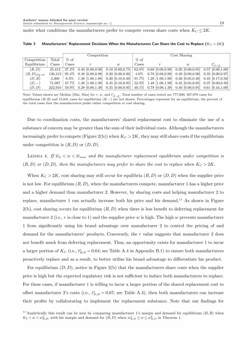
Table 3 Manufacturers’ Replacement Decisions When the Manufacturers Can Share the Cost to Replace (KC < 2K)
Competition Cost SharingCompetition Total % of % ofEquilibrium Cases Cases r w Cases r w t∗s∗1 ,s∗2
(R,D) 25,412 37.2% 0.48 [0.08,0.98] 0.10 [0.00,0.75] 62.8% 0.68 [0.08,0.98] 0.20 [0.00,0.85] 0.57 [0.00,1.00](R,D)D∗
2=0 130,412 95.4% 0.48 [0.08,0.98] 0.20 [0.00,0.90] 4.6% 0.78 [0.08,0.98] 0.40 [0.00,0.90] 0.35 [0.00,0.97]
(D,R) 3,360 8.3% 1.38 [1.08,1.88] 0.20 [0.10,0.40] 91.7% 1.28 [1.08,1.98] 0.20 [0.05,0.40] 0.45 [0.17,0.50](D,−) 71,087 47.7% 1.38 [1.08,1.98] 0.45 [0.10,0.95] 52.3% 1.48 [1.08,1.98] 0.45 [0.05,0.95] 0.37 [0.00,0.50](D,D) 222,910 59.9% 0.28 [0.08,1.38] 0.35 [0.00,0.95] 40.1% 0.78 [0.08,1.38] 0.40 [0.00,0.95] 0.61 [0.44,1.00]
Note: Values shown are Median [Min, Max] for r, w, and t∗s∗1 ,s∗2
. Total number of cases tested are 777,000; 307,978 cases for
equilibrium (R,R) and 15,841 cases for equilibrium (R,−) are not shown. Percentages represent for an equilibrium, the percent ofthe total cases that the manufacturers prefer either competition or cost sharing.
Due to coordination costs, the manufacturers’ shared replacement cost to eliminate the use of a
substance of concern may be greater than the sum of their individual costs. Although the manufacturers
increasingly prefer to compete (Figure 2(b)) whenKC > 2K, they may still share costs if the equilibrium
under competition is (R,D) or (D,D).
Lemma 4. If wL < w < wmax and the manufacturer replacement equilibrium under competition is
(R,D) or (D,D), then the manufacturers may prefer to share the cost to replace when KC > 2K.
When KC > 2K, cost sharing may still occur for equilibria (R,D) or (D,D) when the supplier price
is not low. For equilibrium (R,D), when the manufacturers compete, manufacturer 1 has a higher price
and a higher demand than manufacturer 2. However, by sharing costs and helping manufacturer 2 to
replace, manufacturer 1 can actually increase both his price and his demand.11 As shown in Figure
2(b), cost sharing occurs for equilibrium (R,D) when there is less benefit to deferring replacement for
manufacturer 2 (i.e., r is close to 1) and the supplier price w is high. The high w prevents manufacturer
1 from significantly using his brand advantage over manufacturer 2 to control the pricing of and
demand for the manufacturers’ products. Conversely, the r value suggests that manufacturer 2 does
not benefit much from deferring replacement. Thus, an opportunity exists for manufacturer 1 to incur
a larger portion of KC (i.e., t∗R,D = 0.64; see Table A.4 in Appendix B.1) to ensure both manufacturers
proactively replace and as a result, to better utilize his brand advantage to differentiate his product.
For equilibrium (D,D), notice in Figure 2(b) that the manufacturers share costs when the supplier
price is high but the expected regulatory risk is not sufficient to induce both manufacturers to replace.
For these cases, if manufacturer 1 is willing to incur a larger portion of the shared replacement cost to
offset manufacturer 2’s costs (i.e., t∗D,D = 0.67; see Table A.4), then both manufacturers can increase
their profits by collaborating to implement the replacement substance. Note that our findings for
11 Analytically this result can be seen by comparing manufacturer 1’s margin and demand for equilibrium (R,R) whenwL <w<w
3R,R, with his margin and demand for (R,D) when w1
R,D ≤w≤w2R,D in Theorem 1.
Authors’ names blinded for peer review20 Article submitted to Management Science; manuscript no. ()
equilibria (R,D) and (D,D) are not restricted to KC being only slightly greater than 2K. Examples
exist for both equilibria in which cost sharing occurs when KC is 25 - 50% greater than 2K.
There are a growing number of opportunities for manufacturers to work together to replace sub-
stances of concern. New regulatory initiatives, such as TSCA (Toxic Substances Control Act) reform
in the United States (Rizzuto 2013) and California’s new Safer Consumer Products Regulation (Lee
2013), as well as NGO substance of concern lists such as The SIN “Substitute It Now!” List (The SIN
List 2014) guarantee that the pressure on manufacturers to make difficult decisions regarding the use
of substances of concern in their products will continue to increase in the coming years. For example,
consumer advocacy groups have recently called for the removal of triclosan and phthalates from health
and beauty products (Coolidge 2013, Kary 2014, Koch 2013). Our results in §5 suggest that opportu-
nities exist for manufacturers to collaborate to eliminate the use of a substance of concern. In some
cases the opportunities are intuitive (e.g., a shared cost savings) but in other cases they are not (e.g.,
working together when the shared cost is greater than the sum of the manufacturers’ individual costs).
The key insight, however, is that competing on toxicity does not always make sense for manufacturers
and that collaborating to replace a substance of concern can be a viable option from both an economic
and an environmental perspective.
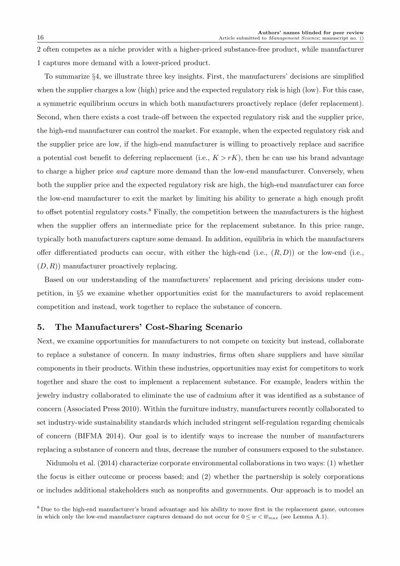
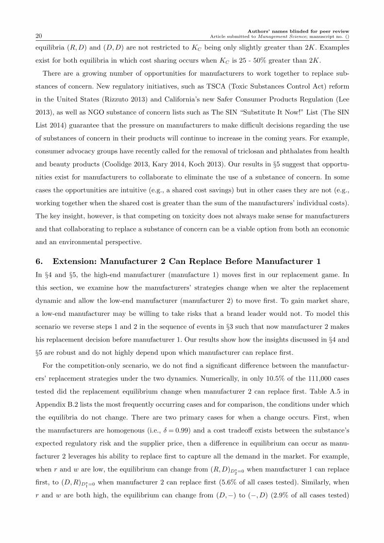
6. Extension: Manufacturer 2 Can Replace Before Manufacturer 1
In §4 and §5, the high-end manufacturer (manufacture 1) moves first in our replacement game. In
this section, we examine how the manufacturers’ strategies change when we alter the replacement
dynamic and allow the low-end manufacturer (manufacturer 2) to move first. To gain market share,
a low-end manufacturer may be willing to take risks that a brand leader would not. To model this
scenario we reverse steps 1 and 2 in the sequence of events in §3 such that now manufacturer 2 makes
his replacement decision before manufacturer 1. Our results show how the insights discussed in §4 and
§5 are robust and do not highly depend upon which manufacturer can replace first.
For the competition-only scenario, we do not find a significant difference between the manufactur-
ers’ replacement strategies under the two dynamics. Numerically, in only 10.5% of the 111,000 cases
tested did the replacement equilibrium change when manufacturer 2 can replace first. Table A.5 in
Appendix B.2 lists the most frequently occurring cases and for comparison, the conditions under which
the equilibria do not change. There are two primary cases for when a change occurs. First, when
the manufacturers are homogenous (i.e., δ = 0.99) and a cost tradeoff exists between the substance’s
expected regulatory risk and the supplier price, then a difference in equilibrium can occur as manu-
facturer 2 leverages his ability to replace first to capture all the demand in the market. For example,
when r and w are low, the equilibrium can change from (R,D)D∗2=0 when manufacturer 1 can replace
first, to (D,R)D∗1=0 when manufacturer 2 can replace first (5.6% of all cases tested). Similarly, when
r and w are both high, the equilibrium can change from (D,−) to (−,D) (2.9% of all cases tested)
Authors’ names blinded for peer reviewArticle submitted to Management Science; manuscript no. () 21
Sup
plie
r P
rice
(w
)
Expected Regulatory Risk (r)10 2
wH
wL
wmax
wD,D
(R,R) (D,R)
(R,R)
(R,-) (D,-)
(D,D)
(R,D)wR,D
(a) Competition Only
Sup
plie
r P
rice
(w
)
Expected Regulatory Risk (r)10 2
wH
wL
wmax
wD,D
(D,R)
(R,R)
(D,-)
(D,D)
(R,D)wR,D
(b) Cost Sharing: KC > 2K
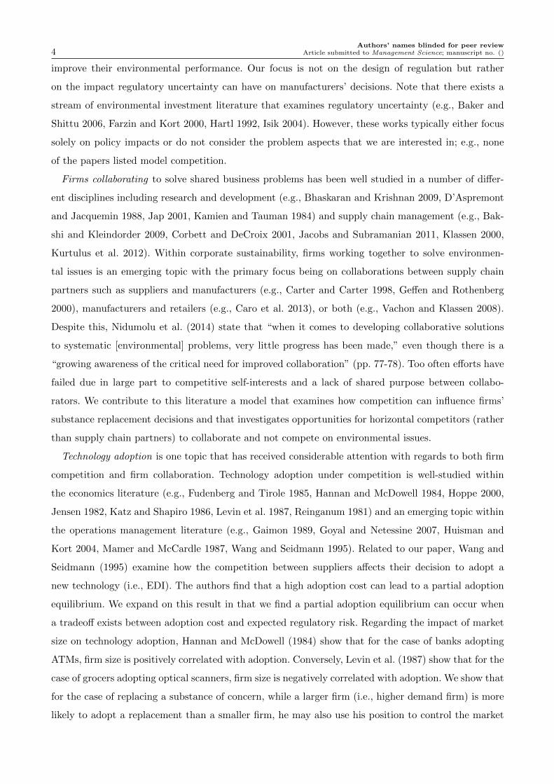
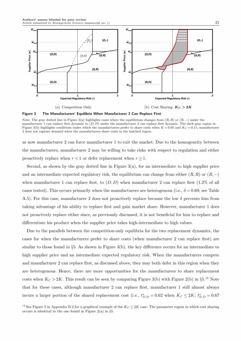
Figure 3 The Manufacturers’ Equilibria When Manufacturer 2 Can Replace First
Note: The gray dotted line in Figure 3(a) highlights cases where the equilibrium changes from (R,R) or (R,−) under themanufacturer 1 can replace first dynamic to (D,D) under the manufacturer 2 can replace first dynamic. The dark gray region inFigure 3(b) highlights conditions under which the manufacturers prefer to share costs when K = 0.05 and KC = 0.11; manufacturer2 does not capture demand when the manufacturers share costs in the hatched region.
as now manufacturer 2 can force manufacturer 1 to exit the market. Due to the homogeneity between
the manufacturers, manufacturer 2 may be willing to take risks with respect to regulation and either
proactively replace when r < 1 or defer replacement when r≥ 1.
Second, as shown by the gray dotted line in Figure 3(a), for an intermediate to high supplier price
and an intermediate expected regulatory risk, the equilibrium can change from either (R,R) or (R,−)
when manufacturer 1 can replace first, to (D,D) when manufacturer 2 can replace first (1.2% of all
cases tested). This occurs primarily when the manufacturers are heterogenous (i.e., δ= 0.69; see Table
A.5). For this case, manufacturer 2 does not proactively replace because the low δ prevents him from
taking advantage of his ability to replace first and gain market share. However, manufacturer 1 does
not proactively replace either since, as previously discussed, it is not beneficial for him to replace and
differentiate his product when the supplier price takes high-intermediate to high values.
Due to the parallels between the competition-only equilibria for the two replacement dynamics, the
cases for when the manufacturers prefer to share costs (when manufacturer 2 can replace first) are
similar to those found in §5. As shown in Figure 3(b), the key difference occurs for an intermediate to
high supplier price and an intermediate expected regulatory risk. When the manufacturers compete
and manufacturer 2 can replace first, as discussed above, they may both defer in this region when they
are heterogenous. Hence, there are more opportunities for the manufacturers to share replacement
costs when KC > 2K. This result can be seen by comparing Figure 3(b) with Figure 2(b) in §5.12 Note
that for these cases, although manufacturer 2 can replace first, manufacturer 1 still almost always
incurs a larger portion of the shared replacement cost (i.e., t∗D,D = 0.62 when KC ≤ 2K; t∗D,D = 0.67
12 See Figure 5 in Appendix B.2 for a graphical example of the KC ≤ 2K case. The parameter region in which cost sharingoccurs is identical to the one found in Figure 2(a) in §5.
Authors’ names blinded for peer review22 Article submitted to Management Science; manuscript no. ()
when KC > 2K). The brand difference between the two manufacturers plays a larger role than the
replacement dynamic in determining the manufacturer that incurs the larger portion of the shared
cost. See Tables A.6 and A.7 in Appendix B.2 for the complete numerical analysis.
7. Managerial Insights and Conclusion
In this paper, we examine how competition influences manufacturers’ strategic decisions when a sub-
stance of concern is identified within their products. To identify ways to increase the number of
manufacturers adopting a replacement, we examine whether manufacturers can avoid competing and
instead, share the cost to replace the substance. We study a vertically differentiated market consisting
of a high-end and a low-end manufacturer selling a product that contains a substance of concern. A
replacement substance is available, but at a higher cost. The manufacturers must decide (1) whether
to proactively replace or to defer replacement and wait to see if regulation occurs and (2) what price to
charge for their products. Our work is motivated by the reusable water bottle industry’s struggles to
replace BPA from their products and by environmentalists’ calls for firms to not compete on toxicity
but instead to collaborate to replace substances of concern. Our results provide insights for manu-
facturers decisions regarding substances of concern, and can act as a starting point for suppliers and
regulators interested in influencing the adoption of safer products by industries.
We find that when manufacturers compete on toxicity, if they do not face a cost tradeoff between
the expected regulatory risk and the supplier price for the replacement substance, then their decisions
are simplified and a symmetric equilibrium occurs in which they either both replace or both defer
replacement. If instead, they face a cost tradeoff, then the high-end manufacturer can use his brand
advantage to control the market. For example, when the expected regulatory risk and the supplier price
are low, if the high-end manufacturer is willing to proactively replace and sacrifice a potential cost
benefit to deferring replacement, then he can charge a higher price and capture more demand than the
low-end manufacturer. Conversely, when the expected regulatory risk and the supplier price are high,
the high-end manufacturer can force the low-end manufacturer to exit the market. The competition
between the manufacturers is highest when the supplier does not price the replacement in one of the
extremes but instead offers an intermediate price. Under these conditions, both manufacturers almost
always capture demand and asymmetric equilibria can occur where either the high-end or the low-end
manufacturer proactively replaces. In addition, a unique equilibrium can occur when consumers’ utility
for the replacement substance is low. Under these conditions, the low-end manufacturer proactively
replaces and is a niche-provider of a higher-priced, substance-free product, while the high-end manufac-
turer ignores his brand advantage and defers replacement to capture more demand with a lower-priced
product containing the substance of concern.
Our results also suggest that competing on toxicity does not always make sense for manufacturers
and that collaborating to replace a substance of concern can be a viable option from both an economic
Authors’ names blinded for peer reviewArticle submitted to Management Science; manuscript no. () 23
and an environmental perspective. When the shared cost to replace a substance is less than manufac-
turers’ individual replacement costs, the low-end manufacturer can use cost sharing to overcome his
brand disadvantage and capture more demand in the market. In addition, opportunities may exist for
manufacturers to collaborate to replace a substance, even when the shared cost to replace is greater than
the sum of the manufacturers’ individual replacement costs. For example, if the manufacturers’ strate-
gies are to differentiate their products with the high-end manufacturer proactively replacing, then the
high-end manufacturer can actually benefit from incurring a large portion of the shared replacement
cost to help the low-end manufacturer replace. This is even though under competition, the high-end
manufacturer can already charge a higher price and capture more demand than the low-end manufac-
turer. Helping the low-end manufacturer to replace, enables the high-end manufacturer to better use
his brand advantage to further increase both his price and his demand, resulting in higher profits.
We develop a stylized model to study the replacement of a substance of concern. In our analysis
we assume that the manufacturers’ replacement costs are symmetric. Numerically, we examine how
our insights change when the replacement costs are asymmetric, with manufacturer 2’s cost being
either less than or greater than manufacturer 1’s cost.13 To test this scenario, we set manufacturer
1’s cost K1 = K and manufacturer 2’s cost K2 = δK or 0.5K when his cost is lower; K2 = K/δ or
2K when his cost is higher. For the competition-only scenario, we do not find a significant difference
when we compare the manufacturers’ replacement strategies for symmetric and asymmetric costs. For
all four K2 costs, the replacement equilibrium changed in less than 5.0% of the 111,000 cases tested.
For the cost sharing scenario, we examine if the manufacturers share costs when KC ≤K1 +K2 and
KC > K1 +K2. Proportionally, cost sharing occurs for a similar percentage of cases as those found
in Tables 3 and A.4. The few differences occur when the asymmetric costs make it difficult to find a
mutually profitable division of KC , and thus, less cost sharing occurs. For example, for equilibrium
(R,D) or (D,D), when KC ≤K1 +K2 and K2 = 0.5K, manufacturer 2 is less likely to share costs (even
though manufacturer 1 incurs a higher portion of KC), since K2 is already low. When KC >K1 +K2,
cost sharing can still occur if the equilibrium under competition is (R,D) or (D,D).
Appendix A: Equilibria Analysis
In this section, we discuss the analysis regarding the manufacturers’ equilibrium replacement strate-
gies and optimal prices. In each scenario, we solve for the subgame perfect Nash equilibrium
[(s∗1, s∗2), p
∗1(s1, s2), p
∗2(s1, s2)] defined as follows.
Definition 2. The strategy profile [(s∗1, s∗2), p
∗1(s1, s2), p
∗2(s1, s2)] constitutes a subgame perfect Nash
equilibrium (SPNE) if it satisfies: (a) For all i∈ {1,2} and given manufacturer −i’s strategy p∗−i(s1, s2),
p∗i (s1, s2)∈ arg maxpi≥0 ΠSi [pi, p
∗−i(s1, s2)], where ΠS
i [·, ·] is manufacturer i’s payoff for replacement equi-
librium S given the two manufacturers’ prices and (b) For all i ∈ {1,2} and given manufacturer −i’s
13 Due to space constraints, we omit the numerical analysis from the paper; it is available from the authors upon request.
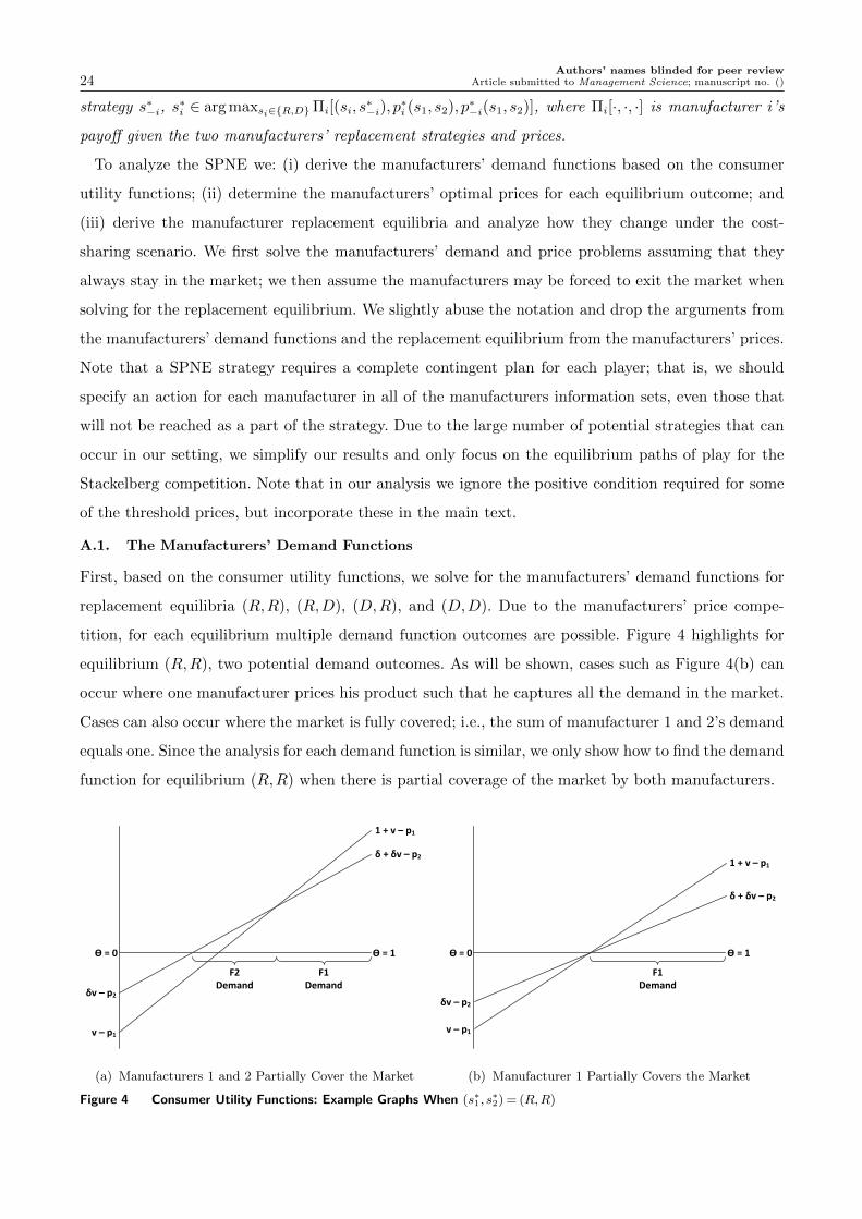
Authors’ names blinded for peer review24 Article submitted to Management Science; manuscript no. ()
strategy s∗−i, s∗i ∈ arg maxsi∈{R,D}Πi[(si, s
∗−i), p
∗i (s1, s2), p
∗−i(s1, s2)], where Πi[·, ·, ·] is manufacturer i’s
payoff given the two manufacturers’ replacement strategies and prices.
To analyze the SPNE we: (i) derive the manufacturers’ demand functions based on the consumer
utility functions; (ii) determine the manufacturers’ optimal prices for each equilibrium outcome; and
(iii) derive the manufacturer replacement equilibria and analyze how they change under the cost-
sharing scenario. We first solve the manufacturers’ demand and price problems assuming that they
always stay in the market; we then assume the manufacturers may be forced to exit the market when
solving for the replacement equilibrium. We slightly abuse the notation and drop the arguments from
the manufacturers’ demand functions and the replacement equilibrium from the manufacturers’ prices.
Note that a SPNE strategy requires a complete contingent plan for each player; that is, we should
specify an action for each manufacturer in all of the manufacturers information sets, even those that
will not be reached as a part of the strategy. Due to the large number of potential strategies that can
occur in our setting, we simplify our results and only focus on the equilibrium paths of play for the
Stackelberg competition. Note that in our analysis we ignore the positive condition required for some
of the threshold prices, but incorporate these in the main text.
A.1. The Manufacturers’ Demand Functions
First, based on the consumer utility functions, we solve for the manufacturers’ demand functions for
replacement equilibria (R,R), (R,D), (D,R), and (D,D). Due to the manufacturers’ price compe-
tition, for each equilibrium multiple demand function outcomes are possible. Figure 4 highlights for
equilibrium (R,R), two potential demand outcomes. As will be shown, cases such as Figure 4(b) can
occur where one manufacturer prices his product such that he captures all the demand in the market.
Cases can also occur where the market is fully covered; i.e., the sum of manufacturer 1 and 2’s demand
equals one. Since the analysis for each demand function is similar, we only show how to find the demand
function for equilibrium (R,R) when there is partial coverage of the market by both manufacturers.
F2 Demand
F1 Demand
δv – p2
v – p1
δ + δv – p2
1 + v – p1
Ɵ = 1Ɵ = 0
(a) Manufacturers 1 and 2 Partially Cover the Market
δv – p2
v – p1
δ + δv – p2
1 + v – p1
Ɵ = 1Ɵ = 0
F1 Demand
(b) Manufacturer 1 Partially Covers the Market
Figure 4 Consumer Utility Functions: Example Graphs When (s∗1, s∗2) = (R,R)
Authors’ names blinded for peer reviewArticle submitted to Management Science; manuscript no. () 25
For equilibrium (R,R), let v − p1 < δv − p2 < 0, δ + δv − p2 < 1 + v − p1, and p2 < δp1. These
conditions ensure that there is partial coverage of the market by both manufacturers. Setting the
consumer’s utility for manufacturer 1 and 2 equal to each other, we find that the consumer is indifferent
between the manufacturers at θ1 = ((p1 − p2)− v(1− δ))/(1− δ). Thus, manufacturer 1 captures all
consumers for θ1 ≤ θ≤ 1; i.e., d1 = 1 +v− (p1−p2)/(1− δ). Similarly, setting the consumer’s utility for
manufacturer 2 equal to 0, we find that the consumer is indifferent between manufacturer 2 and not
purchasing at θ2 = (p2/δ)− v. Thus, manufacturer 2 captures all consumers for θ2 ≤ θ < θ1; i.e., d2 =
θ1−θ2 = (δp1−p2)/(δ(1− δ)). Consumers between 0≤ θ < θ2 do not purchase the product. Applying a
similar analysis, we can show that if there is full coverage of the market by both manufacturers, then
d1 = 1 + v− (p1 − p2)/(1− δ) and d2 = (p1 − p2)/(1− δ)− v. If instead, only manufacturer 1 captures
demand, then d1 = 1 + v− p1 and d2 = 0 with manufacturer 1 partially covering the market.
Next, we define the possible manufacturer demand functions for the remaining replacement equilibria.
Which demand functions occur depends on the manufacturers’ price competition and will be shown
in §A.2. For equilibrium (R,D), a similar analysis demonstrates that the manufacturers’ demand
functions are d1 = 1−((p1−p2)−v)/(1−δ) and d2 = (δp1−p2−v)/(δ(1−δ)) when both manufacturers
partially cover the market; d1 = 1− ((p1− p2)− v)/(1− δ) and d2 = ((p1− p2)− v)/(1− δ) when both
manufacturers fully cover the market; d1 = 1 and d2 = 0 when manufacturer 1 fully covers the market;
and d1 = 0 and d2 = 1− (p2/δ) when manufacturer 2 partially covers the market.
For equilibrium (D,R), the manufacturers’ demand functions are d1 = 1− ((p1 − p2) + δv)/(1− δ)
and d2 = (δp1−p2 +δv)/(δ(1−δ)) when both manufacturers partially cover the market; d1 = 1− ((p1−
p2) + δv)/(1− δ) and d2 = ((p1 − p2) + δv)/(1− δ) when both manufacturers fully cover the market;
d1 = 0 and d2 = 1 when manufacturer 2 fully covers the market; and d1 = 1 − p1 and d2 = 0 when
manufacturer 1 partially covers the market.
For equilibrium (D,D), the manufacturers’ decisions are independent of w and v. Therefore, both
manufacturers always partially cover the market. The manufacturers’ demand functions are d1 = 1−
(p1− p2)/(1− δ) and d2 = (δp1− p2)/(δ(1− δ)). �
A.2. The Manufacturers’ Pricing Decisions
Next, based on the manufacturers’ demand functions, we solve for the manufacturers’ optimal prices
for each potential replacement equilibrium.
Proof of Theorem 1: We solve for the manufacturers’ optimal prices and resulting payoffs for
equilibria: (R,R), (R,D), (D,R), and (D,D). Since the analysis for each equilibrium is similar, we
only show our analysis for equilibrium (R,R). First, we solve for the manufacturers’ optimal prices
when the price competition results in both manufacturers either partially or fully covering the market.
We then solve for the manufacturers’ optimal prices when only one manufacturer captures demand.
For equilibrium (R,R), first consider the case when the price competition results in both manufac-
turers partially covering the market. For this to occur, the following constraints must hold: v− p1 <
Authors’ names blinded for peer review26 Article submitted to Management Science; manuscript no. ()
δv− p2 < 0, δ+ δv− p2 < 1 + v− p1, p2 < δp1, δ+ δv− p2 ≥ 0, p1 ≥ 0, and p2 ≥ 0. Based on the solution
for the manufacturers’ demand functions, manufacturer 1 and 2’s payoffs are
ΠR,R1 (p1, p2) = (1 + v− (p1− p2)/(1− δ))(p1−w)−K, and (6)
ΠR,R2 (p2, p1) = ((δp1− p2)/(δ(1− δ)))(p2−w)−K. (7)
Taking the derivative of manufacturer 1’s payoff with respect to p1 and solving, we find that p∗1 =
((1− δ) + p∗2 +w+ v(1− δ))/2. Similarly, p∗2 = (w+ δp∗1)/2. Solving for p∗1 and p∗2 we find
p∗1 = [2(1− δ)(1 + v) + 3w]/(4− δ), and
p∗2 = [δ(1− δ)(1 + v) +w(2 + δ)]/(4− δ).
Inserting p∗1 and p∗2 into (6) and (7), we find
ΠR,R1 (p∗1, p
∗2) = [(2(1 + v)−w)(1− δ)]2/[(1− δ)(4− δ)2]−K, and
ΠR,R2 (p∗2, p
∗1) = [(δ(1 + v)− 2w)(1− δ)]2/[δ(1− δ)(4− δ)2]−K.
Based on the manufacturers’ optimal prices and the demand constraints, this outcome occurs for w
values such that w2R,R <w<w
3R,R with w2
R,R = [3δv− δ(1− δ)]/(2 + δ) and w3R,R = δ(1 + v)/2.
For the case when both manufacturers fully cover the market, we apply a similar analysis. For this
case to occur, the following constraints are necessary: v−p1 < δv−p2, 0≤ δv−p2, δ+δv−p2 < 1+v−p1,
p1 ≥ 0, and p2 ≥ 0. Solving for p∗1 and p∗2 we find
p∗1 = w+ (1− δ)(2 + v)/3, and
p∗2 = w+ (1− δ)(1− v)/3.
The manufacturers’ payoffs are then
ΠR,R1 (p∗1, p
∗2) = ((2 + v)2)(1− δ)/9−K, and
ΠR,R2 (p∗2, p
∗1) = ((1− v)2)(1− δ)/9−K.
Based on the manufacturers’ optimal prices and the demand constraints, this outcome occurs for w
values such that 0≤w≤w1R,R with w1
R,R = [v(1 + 2δ)− (1− δ)]/3.
For w ≥ w3R,R, demand constraint p2 < δp1 no longer holds for the both manufacturers partially
covering the market solution. Due to the high supplier price, manufacturer 1 can set a price such that
manufacturer 2 must set p∗2 = w and no longer captures demand; i.e., only manufacturer 1 captures
demand (with partial coverage). For w3R,R ≤w<w4
R,R ≡ δ(1 +v)/(2− δ), constraint p2 < δp1 binds and
thus, p∗1 = w/δ. The manufacturers’ payoffs are then ΠR,R1 (p∗1, p
∗2) = [w(1− δ)(δ(1 + v)−w)]/δ2 −K;
ΠR,R2 (p∗2, p
∗1) =−K. For w4
R,R ≤w≤wmaxR,R ≡ δ(1 + v), p∗1 = (1 + v+w)/2 as manufacturer 1 charges the
monopoly profit maximizing price (and not the higher w/δ price). The manufacturers’ payoffs are then
Authors’ names blinded for peer reviewArticle submitted to Management Science; manuscript no. () 27
ΠR,R1 (p∗1, p
∗2) = (1 + v − w)2/4−K; ΠR,R
2 (p∗2, p∗1) = −K. Note that wmaxR,R is the highest supplier price
such that there is at least some positive utility for both consumer utility functions.
For w1R,R < w ≤ w2
R,R, demand constraint 0≤ δv − p2 (full coverage case) binds and constraint 0>
δv− p2 (partial coverage case) no longer holds. For the full (partial) coverage case, manufacturer 2’s
best response is to decrease (increase) his price such that p∗2 = δv, which ensures that the market
is fully covered. Given p∗2, manufacturer 1’s best response is to set p∗1 = [(1 − δ) + (w + v)]/2. The
manufacturers’ payoffs are then ΠR,R1 (p∗1, p
∗2) = [(1− δ) + (v −w)]2/(4(1− δ))−K and ΠR,R
2 (p∗2, p∗1) =
[(1− δ)− (v−w)](δv−w)/[2(1− δ)]−K.
For equilibrium (R,D), a similar analysis shows that for 0≤ w <w1R,D ≡ v− (1− δ), manufacturer
1 fully covers the market with p∗1 = v, p∗2 = 0, ΠR,D1 (p∗1, p
∗2) = v − w −K, and ΠR,D
2 (p∗2, p∗1) = −rK.
For w1R,D ≤ w ≤ w2
R,D ≡ [v(2− δ)− δ(1− δ)]/δ, both manufacturers partially cover the market with
p∗1 = [(1−δ)+(v+w)]/2, p∗2 = 0, ΠR,D1 (p∗1, p
∗2) = (1−δ+v−w)2/[4(1−δ)]−K, and ΠR,D
2 (p∗2, p∗1) =−rK.
For w2R,D < w < w3
R,D ≡ [v + 2(1 − δ)]/(2 − δ), both manufacturers partially cover the market with
p∗1 = [2(1− δ) + (v+ 2w)]/(4− δ), p∗2 = [δ((1− δ) + v+w)− 2v]/(4− δ), ΠR,D1 (p∗1, p
∗2) = [2(1− δ) + v−
w(2− δ)]2/[(1− δ)(4− δ)2]−K, and ΠR,D2 (p∗2, p
∗1) = [2v− δ((1− δ) + v+w)]2/[δ(1− δ)(4− δ)2]− rK.
For w3R,D ≤ w < w4
R,D ≡ (1 + v)− δ/2, manufacturer 2 partially covers the market with p∗1 = w, p∗2 =
(δ + w) − (1 + v), ΠR,D1 (p∗1, p
∗2) = −K, and ΠR,D
2 (p∗2, p∗1) = [(1 + v − w)((w − v) − (1 − δ))]/δ − rK.
Finally, for w4R,D ≤w≤wmaxR,D ≡ 1+v, manufacturer 2 partially covers the market with p∗1 =w, p∗2 = δ/2,
ΠR,D1 (p∗1, p
∗2) =−K, and ΠR,D
2 (p∗2, p∗1) = δ/4− rK.
For equilibrium (D,R), a similar analysis shows that for 0≤w<w1D,R ≡ δv−2(1−δ), manufacturer 2
fully covers the market with p∗1 = 0, p∗2 = δv− (1− δ), ΠD,R1 (p∗1, p
∗2) =−rK, and ΠD,R
2 (p∗2, p∗1) = δv− (1−
δ)−w−K. For w1D,R ≤w≤w2
D,R ≡ δv− (1− δ)/2, both manufacturers partially cover the market with
p∗1 = [2(1− δ)+w− δv]/3, p∗2 = [(1− δ)+2w+ δv]/3, ΠD,R1 (p∗1, p
∗2) = [2(1− δ)+w− δv]2/[9(1− δ)]− rK,
and ΠD,R2 (p∗2, p
∗1) = [(1− δ)−w+ δv]2/[9(1− δ)]−K. For w2
D,R <w<w3D,R ≡ δv+ δ(1− δ)/(2− δ), both
manufacturers partially cover the market with p∗1 = [2(1−δ)+w−δv]/(4−δ), p∗2 = [δ(1−δ)+δv(2−δ)+
2w]/(4− δ), ΠD,R1 (p∗1, p
∗2) = [2(1− δ) +w− δv]2/[(1− δ)(4− δ)2]− rK, and ΠD,R
2 (p∗2, p∗1) = [−w(2− δ) +
δ((1− δ) +v(2− δ))]2/[δ(1− δ)(4− δ)2]−K. For w3D,R ≤w<w4
D,R ≡ δ/2 + δv, manufacturer 1 partially
covers the market with p∗1 = (w− δv)/δ, p∗2 =w, ΠD,R1 (p∗1, p
∗2) = [(w− δv)(δ(1 + v)−w)]/δ2− rK, and
ΠD,R2 (p∗2, p
∗1) =−K. Finally, for w4
D,R ≤w≤wmaxD,R ≡ δ(1+v), manufacturer 1 partially covers the market
with p∗1 = 1/2, p∗2 =w, ΠD,R1 (p∗1, p
∗2) = 1/4− rK, and ΠD,R
2 (p∗2, p∗1) =−K.
For equilibrium (D,D), both manufacturers always partially cover the market. Solving for the man-
ufacturers’ optimal prices and payoffs we find that p∗1 = 2(1− δ)/(4− δ) and p∗2 = δ(1− δ)/(4− δ), with
ΠD,D1 (p∗1, p
∗2) = 4(1− δ)/(4− δ)2− rK and ΠD,D
2 (p∗2, p∗1) = δ(1− δ)/(4− δ)2− rK. �
Proof of Corollary 1: Corollary 1 follows directly from Theorem 1. �
Proof of Lemma 1: The proof follows directly from Theorem 1 by comparing the manufacturers’
prices and demands for equilibria (R,R), (R,D), (D,R), and (D,D). Threshold prices wR,D = (δ(1−
δ) + 2v)/[δ(3− δ)] and wD,R = δv− δ(1− δ)/2 are found by calculating the w at which D∗1 =D∗2. �
Authors’ names blinded for peer review28 Article submitted to Management Science; manuscript no. ()
A.3. The Manufacturers’ Replacement Decisions
Given the manufacturers’ optimal prices, we next solve for the manufacturers’ replacement strategies.
Proof of Theorems 2.A and 2.B: In order to limit the number of cases such that either a
symmetric equilibrium occurs or only one manufacturer captures demand, we restrict the supplier
price range to 0 ≤ w < wmax ≡min{
max{δ(1+v)
2, v+2(1−δ)
2−δ
}, δv+ δ
2
}and consumer utility to 0 ≤ v <
min{δ, δ(2−δ)
4−2δ−2δ2
}. We examine three cases: the supplier price is low, intermediate, or high. For each
case, we (i) order the supplier threshold prices defined in Theorem 1; (ii) define manufacturer 2’s best
response functions if manufacturer 1 defers or replaces; (iii) define manufacturer 1’s best response func-
tions; and (iv) compare manufacturer 1 and 2’s best response functions to determine the replacement
equilibrium. Note that when analyzing the replacement equilibrium, we break the indifference point in
favor of R. To simplify our exposition, we define the following terms.
Utility bounds: v1 = δ/(2(2 + δ)), v2 = δ/(3 + δ), v3 = δ/(2(1 + δ)), v4 = 2δ/((2− δ)(2 + δ)), v5 = δ(2−
δ)/(4− 2δ− δ2), v6a = δ(2− δ)/(4− 2δ− 2δ2), v6b = δ/(2− δ), va = [δ(2− δ)− 4(1− δ)]/[2(1− δ) + δ2],
and vb = [δ(2− δ)− 4(1− δ)]/[2(1− δ)2].
Manufacturer 2’s Best Response: If manufacturer 1 defers (i.e., s1 =D), then we define
• Y 1(w) = 1 + δ(1− δ)/[K(4− δ)2] for w3D,R ≤w<wmax,
• Y 2(w) = 1− [2δ(1− δ) + (2− δ)(δv−w)](δv−w)(2− δ)/[δK(1− δ)(4− δ)2] for w2D,R <w<w
3D,R,
• Y 3(w) = 1 + δ(1− δ)/[K(4− δ)2]− [(1− δ)− (w− v)]2/[9K(1− δ)] for w1D,R ≤w≤w2
D,R,
• Y 4(w) = 1 + δ(1− δ)/[K(4− δ)2] + [(1− δ) + (w− δv)]/K for 0≤w<w1D,R,
such that manufacturer 2’s best response is s2 =R if r≥ Y j(w), and s2 =D otherwise.
If manufacturer 1 replaces (i.e., s1 =R), then we define
• X1(w) = 1 + [δ(1 − δ) + δw − v(2 − δ)]2/[δK(1 − δ)(4 − δ)2] for max{w2R,D,w
3R,R} < w <
min{w3R,D,w
4D,R},
• X2(w) = 1− [(2w− δ(1 + v))2](1− δ)/(δK(4− δ)2)− [(1 + v−w)2− δ(1 + v−w)]/[δK] for w3R,D ≤
w<w3R,R,
• X3(w) = 1− [2(v +w)− δ(2 + 2v + 3w) + δ2(2 + v)][w(2− δ)− v(2− δ2)]/[δK(1− δ)(4− δ)2] for
max{w2R,D,w
3D,R} ≤w<min{w3
R,D,w3R,R},
• X4(w) = 1− [(2w− δ(1 + v))2](1− δ)/[δK(4− δ)2] for w3D,R <w<min{w2
R,D,w3R,R},
• X5(w) = 1− (δv−w)[(1−δ)+(w−v)]/(2K(1−δ))+[δ(1−δ)+δw−v(2−δ)]2/[δK(1−δ)(4−δ)2]
for max{w2R,D,w
1R,R}<w≤w2
R,R,
• X6(w) = 1− (δv−w)[(1− δ) + (w− v)]/[2K(1− δ)] for w1R,R <w≤min{w2
R,D,w2R,R},
• X7(w) = 1−(1−δ)(1−v)2/9K+[δ(1−δ)+δw−v(2−δ)]2/[δK(1−δ)(4−δ)2] for w2R,D <w≤w1
R,R,
• X8(w) = 1− (1− δ)(1− v)2/9K for 0≤w≤min{w2R,D,w
1R,R},
such that manufacturer 2’s best response is s2 =R if r≥Xj(w), and s2 =D otherwise.
Low Supplier Price: We define 0≤w≤w2R,R as the low supplier price range. For this range, ordering
the (R,R), (R,D), and (D,R) threshold prices, we find that w1D,R < w1
R,D < w2D,R < w1
R,R < w2R,R
Authors’ names blinded for peer reviewArticle submitted to Management Science; manuscript no. () 29
with two exceptions. First, the ordering of w2R,D depends on v: w1
R,D < w2R,D < w2
D,R if 0 ≤ v < v1;
w2D,R ≤w2
R,D <w1R,R if v1 ≤ v < v2; w1
R,R ≤w2R,D <w
2R,R if v2 ≤ v < v3; and w1
R,R ≤w2R,D if v3 ≤ v < v6a.
Second, for v3 ≤ v < v6a, if v≥ 1/2, then w2D,R <w
1R,D, with w2
D,R <w1R,D always holding if v6b ≤ v < v6a
and δ≥ 2/3 and w1R,D <w
2D,R always holding if v5 ≤ v < v6a and δ < 2/3.
Next, based on the ordering of supplier threshold prices, we analyze manufacturer 2’s best response
given manufacturer 1’s strategy s1 ∈ {D,R}. If s1 =D, then for (ia) 0≤ w < w1D,R, manufacturer 2’s
best response is to replace if r≥ Y 4(w), and to defer otherwise; (iia) w1D,R ≤w≤w2
D,R, manufacturer 2’s
best response is to replace if r≥ Y 3(w), and to defer otherwise; (iiia) w2D,R <w≤w2
R,R, manufacturer
2’s best response is to replace if r ≥ Y 2(w), and to defer otherwise. If s1 = R, then for (ib) 0≤ w ≤
min{w2R,D,w
1R,R}, manufacturer 2’s best response is to replace if r ≥X8(w), and to defer otherwise;
(iib) w2R,D <w≤w1
R,R, manufacturer 2’s best response is to replace if r≥X7(w), and to defer otherwise;
(iiib) max{w2R,D,w
1R,R}<w≤w2
R,R, manufacturer 2’s best response is to replace if r ≥X5(w), and to
defer otherwise; and (ivb) w1R,R <w ≤min{w2
R,D,w2R,R}, manufacturer 2’s best response is to replace
if r≥X6(w), and to defer otherwise.
Finally, we determine manufacturer 1’s best responses and the resulting replacement equilibrium.
Over the range of supplier threshold prices, we first determine the possible equilibrium combinations
that manufacturer 2 may prefer. When s1 = R, the possible equilibria are (R,R) or (R,D); when
s1 = D, the possible equilibria are (D,R) or (D,D). Based on how manufacturer 2’s best response
functions align, we can determine the two equilibria manufacturer 1 selects from and thus, manufacturer
1’s best response functions. Due to the number of possible comparisons that must be made (both
between manufacturer 2’s best response function and in determining manufacturer 1’s best response),
we present a sample case with the full analysis available upon request from the authors.
For w1D,R ≤w<w1
R,D, manufacturer 2’s best responses are if s1 =D, to replace if r≥ Y 3(w), and to
defer otherwise; and if s1 = R, to replace if r ≥X8(w), and to defer otherwise. These best response
functions hold for 0≤ v < v6a.14 Comparing the functions, we find that Y 3(w)<X8(w). Therefore, the
possible replacement equilibria given s1 = R or s1 = D are (R,D) and (D,D) for r < Y 3(w), (R,D)
and (D,R) for Y 3(w)≤ r <X8(w), and (R,R) and (D,R) for X8(w)≤ r.
Based on manufacturer 2’s best responses and the threshold prices, we calculate manufacturer
1’s best responses. Define Z1(w, (s1, s2) = (R,D) or (D,D)) = 1 − (1/K)[(v − w) − 4(1 − δ)/(4 −
δ)2], Z2(w, (s1, s2) = (R,D) or (D,R)) = 1 − (1/K)[(v − w) − (2 + w − δ(2 + v))2/(9(1 − δ))], and
Z3(w, (s1, s2) = (R,R) or (D,R)) = 1− [(v − w)(4 + v + w − 2δ(2 + v))]/(9K(1− δ)). For r < Y 3(w),
manufacturer 1 replaces if r ≥ Z1(w, (R,D) or (D,D)), and defers otherwise. For Y 3(w) ≤ r <
X8(w), manufacturer 1 replaces if r ≥ Z2(w, (R,D) or (D,R)), and defers otherwise. For X8(w) ≤
r, manufacturer 1 replaces if r ≥ Z3(w, (R,R) or (D,R)), and defers otherwise. Comparing man-
ufacturer 1’s best responses to Y 3(w) and X8(w), we find that Z3(w, (R,R) or (D,R)) < X8(w),
14 Note that this is not always the case. The manufacturers’ best response functions often depend on both v and w.
Authors’ names blinded for peer review30 Article submitted to Management Science; manuscript no. ()
Z2(w, (R,D) or (D,R))<Y 3(w), and Z1(w, (R,D) or (D,D))<Y 3(w). Based on these conditions, for
w1D,R ≤w<w1
R,D, the manufacturer replacement equilibrium given r is
(s∗1, s∗2) =
(D,D) if r <Z1(w, (R,D) or (D,D)),
(R,D) if Z1(w, (R,D) or (D,D))≤ r <X8(w),
(R,R) if r≥X8(w).
Following a similar analysis, we can construct the replacement equilibrium for the low supplier price
range. For 0≤w<w2R,R, the manufacturer replacement equilibrium given r is
(s∗1, s∗2) =
(D,D) if r < F1(w),
(R,D) if F1(w)≤ r < F2(w),
(R,R) if r≥ F2(w),
(8)
with the exception that for 0≤ v < v1 and w2D,R <w ≤ w2
R,R, if min{F3(w),F5(w)}> F2(w), then the
manufacturer replacement equilibrium given r is
(s∗1, s∗2) =
(D,D) if r < F1(w),
(R,D) if F1(w)≤ r < F2(w),
(D,D) if F2(w)≤ r <min{F3(w),F5(w)},
(R,R) if r≥min{F3(w),F5(w)}.
(9)
We define F2(w) =Xj(w) as defined above. We define F1(w) equal to: 1− ((1− δ) + (v−w))2/4K(1−
δ) + 4(1 − δ)/(K(4 − δ)2) for w1R,R < w ≤ min{w2
R,R,w2R,D}; 1 − (v − w(2 − δ))(4 + v − w(2 − δ) −
4δ)/(K(1 − δ)(4 − δ)2) for max{w1R,R,w
2R,D} < w ≤ w2
R,R; 1 − (v − w(2 − δ))(4(1 − δ) + v − w(2 −
δ))/(K(1−δ)(4−δ)2) for w2R,D <w≤w1
R,R; 1− (v−w)/K+(4(1−δ))/K(4−δ)2 for 0≤w<w1R,D; and
1+4(1−δ)/K(4−δ)2−((1−δ)+(v−w))2/(4K(1−δ)) for w1R,D ≤w<min{w2
R,D,w1R,R}. For Equation
(9), F3(w) = Y 2(w) and F5(w) = 1− (1− δ)(2 + v)2/9K + 4(1− δ)/(K(4− δ)2) for w2D,R < w ≤ w1
R,R
and F5(w) = 1− ((1− δ)+(v−w))2/(4K(1− δ))+4(1− δ)/(K(4− δ)2) for w1R,R <w≤w2
R,R. Note that
manufacturer 2 may or may not capture demand for equilibrium (R,D) (see Theorem 1).
High Supplier Price: We apply a similar analysis to analyze the high supplier price case. We define
w3D,R ≤w<min{max{w3
R,R,w3R,D},w4
D,R} as the high supplier price range. Ordering the (R,R), (R,D),
and (D,R) threshold prices, we find that for 0≤ v < v4, w3D,R <w3
R,D <w3R,R if v < va, w
3D,R <w3
R,R <
w3R,D if va ≤ v < vb, and w3
D,R <w3R,R <w
4D,R <w
3R,D if vb ≤ v. For v4 ≤ v < v5, additionally we find that
w3D,R <w
2R,D <min{w3
R,R,w3R,D}. For v5 ≤ v < v6a, if δ < 2/3, then w3
D,R <w3R,R <w
2R,D <w
4D,R <w
3R,D.
If instead, δ ≥ 2/3, then for v5 ≤ v < v6b, w3D,R < w3
R,R < w2R,D < w3
R,D and for v6b ≤ v < v6a, w3D,R <
w2R,D <w
3R,D. For both cases, w2
R,D <w4D,R <w
3R,D if v≥ vb.
Next, based on the ordering of supplier threshold prices, we analyze manufacturer 2’s best response
given manufacturer 1’s strategy s1 ∈ {D,R}. If s1 =D, then manufacturer 2’s best response is to replace
if r≥ Y 1(w), and to defer otherwise. If s1 =R, then for (i) max{w2R,D,w
3D,R} ≤w <min{w3
R,R,w3R,D},
manufacturer 2’s best response is to replace if r ≥ X3(w), and to defer otherwise; (ii) w3R,D ≤
Authors’ names blinded for peer reviewArticle submitted to Management Science; manuscript no. () 31
w < w3R,R, manufacturer 2’s best response is to replace if r ≥ X2(w), and to defer otherwise; (iii)
max{w2R,D,w
3R,R}< w <min{w3
R,D,w4D,R}, manufacturer 2’s best response is to replace if r ≥X1(w),
and to defer otherwise; (iv) w3D,R ≤w<min{w2
R,D,w3R,R}, manufacturer 2’s best response is to replace
if r ≥ X4(w), and to defer otherwise; and (v) max{w3D,R,w
3R,R} ≤ w ≤ w2
R,D, manufacturer 2’s best
response is to replace if r≥ 1, and to defer otherwise.
Finally, we determine manufacturer 1’s best responses and the resulting replacement equilibrium.
Following a similar analysis to the low supplier price case, we can determine the possible equilibria
combinations that manufacturer 2 may prefer over the range of threshold prices. Then, based on how
manufacturer 2’s best response functions align, we can determine the equilibria manufacturer 1 selects
from and thus, manufacturer 1’s best responses.
For the high supplier price range (i.e., w3D,R ≤w <min{max{w3
R,R,w3R,D},w4
D,R}), if F2(w)≥ F3(w)
OR F2(w)< F3(w), F3(w)< F5(w), and 0≤ v < δ3+δ
, then the manufacturer replacement equilibrium
given r is
(s∗1, s∗2) =
(D,D) if r < F3(w),
(D,R) if F3(w)≤ r < F4(w),
(R,R) if r≥ F4(w).
(10)
If instead, F2(w)< F3(w) AND F3(w)≥ F5(w) and 0≤ v < δ3+δ
OR F3(w)≤ F4(w) and δ3+δ≤ v < v,
then the manufacturer replacement equilibrium given r is
(s∗1, s∗2) =
(D,D) if r <max{F2(w),F5(w)},
(R,R) if max{F2(w),F5(w)} ≤ r < F3(w),
(D,R) if F3(w)≤ r < F4(w),
(R,R) if r≥ F4(w).
(11)
Finally, if F2(w)< F3(w), F3(w)> F4(w), and δ3+δ≤ v < v, then the manufacturer replacement equi-
librium given r is
(s∗1, s∗2) =
{(D,D) if r < F3(w),
(R,R) if r≥ F3(w).(12)
We define F3(w) = Y 1(w) and F2(w) = Xj(w) as defined above. For w3D,R ≤ w < w3
R,R, F4(w) = 1−
(1− δ)(2(1 + v)−w)2/(K(4− δ)2)− (w− δv)(w− δ(1 + v))/(δ2K) and F5(w) = 1− (2v−w)(4 + 2v−
w)(1− δ)/(K(4− δ)2). For max{w3R,R,w
3D,R} ≤w <w3
R,D, F4(w) = 1− ((v−w)(−w+ δ(1 + v)))/(δK)
and F5(w) = 1 + 4(1− δ)/K(4− δ)2 +w(1− δ)(w− δ(1 + v))/(δ2K).
Note that manufacturer 2 does not capture demand for equilibrium (D,R) and may or may not
capture demand for equilibrium (R,R) (see Theorem 1). By Assumption 3, a manufacturer is forced to
exit the market if his best response payoff is less than or equal to −K. For equilibria (D,R) and (R,R)
(when manufacturer 2 does not capture demand), manufacturer 2’s payoff equals −K. This implies
that his next best payoff (i.e., (D,D) and (R,D)) are less than −K. As such, he cannot earn more
than −K and is forced to exit the market for these cases. We therefore update equilibrium (D,R) to
(D,−) and equilibrium (R,R) to (R,−) (when manufacturer 2 does not capture demand).
Authors’ names blinded for peer review32 Article submitted to Management Science; manuscript no. ()
Intermediate Supplier Price: Applying a similar analysis to analyze the intermediate supplier price
case, we define w2R,R ≤ w < w3
D,R as the intermediate supplier price range. Ordering the threshold
prices, we find that w2R,R <w3
D,R are the only two threshold prices, except when w2R,R <w2
R,D <w3D,R
for v3 ≤ v < v4 and w2R,R <w
3R,R <w
3D,R for v6b ≤ v < v6a and δ≥ 2/3.
Next, we analyze manufacturer 2’s best response given manufacturer 1’s strategy s1 ∈ {D,R}. If
s1 =D, then manufacturer 2’s best response is to replace if r≥ Y 2(w), and to defer otherwise. If s1 =R,
then for (i) max{w2R,D,w
2R,R}<w < w3
D,R, manufacturer 2’s best response is to replace if r ≥X3(w),
and to defer otherwise; (ii) w2R,R < w < min{w2
R,D,w3R,R,w
3D,R}, manufacturer 2’s best response is to
replace if r≥X4(w), and to defer otherwise; and (iii) w3R,R ≤w<w3
D,R, manufacturer 2’s best response
is to replace if r≥ 1, and to defer otherwise.
Finally, we determine manufacturer 1’s best responses and the resulting replacement equilibrium.
Our analysis is restricted since we cannot easily define when one manufacturer’s best response function
is greater than another. We analyze the remainder of the replacement equilibrium numerically. �
Lemma A.1. For 0≤w<wmax, when manufacturer 1 moves before manufacturer 2 in the replace-
ment game, manufacturer 2 cannot be the only manufacturer to capture demand in the market.
Proof: The proof follows directly from Theorems 2.A and 2.B.
Proof of Lemma 2: We examine when the manufacturers’ replacement equilibrium is always (R,R)
when the supplier price is low. By Theorem 2.A and Equation (8), we know that if r≥ 1 and w1D,R ≤
w<min{w2R,D,w
1R,R}, then (s∗1, s
∗2) = (R,R). For 0≤w<w1
D,R, if manufacturer 1 replaces (i.e, s1 =R),
then manufacturer 2’s best response is to replace since under equilibrium (R,D), only manufacturer 1
captures demand for this supplier price range. If manufacturer 1 defers (i.e, s1 =D), then manufacturer
2’s best response is to replace. This can be shown by comparing manufacturer 2’s profits when (s∗1, s∗2) =
(D,R) and (D,D). Thus, manufacturer 1 selects between equilibria (R,R) and (D,R). Manufacturer
1’s best response is to replace since only manufacturer 2 captures demand under equilibrium (D,R) and
this supplier price range. For supplier price range min{w2R,D,w
1R,R} ≤w≤w2
R,R, we can show that for
Equation (8), F2(w)< 1 over the following ranges: w2R,D <w ≤w1
R,R and 0≤ v < v2; w1R,R <w ≤w2
R,R
and 0≤ v < v2; w2R,D <w ≤ w2
R,R and v2 ≤ v < v3; w1R,R <w ≤ w2
R,D and v2 ≤ v < v3; and w1R,R <w ≤
w2R,R and v3 ≤ v < v6a. In addition, it can be shown that for the exception case (Equation (9)), both
F3(w) and F5(w) are less than 1 for w2D,R <w≤w2
R,R and 0≤ v < v1. Hence, if r≥ 1 and 0≤w≤w2R,R,
the manufacturers’ replacement equilibrium is always (R,R).
The proof of the (R,D) result follows directly from Theorem 2.A.
Next, we examine when the manufacturers’ replacement equilibrium is always (D,D) when the sup-
plier price is high. If manufacturer 1 defers replacement, then manufacturer 2’s best response for w3D,R ≤
w≤wmaxD,R is to defer since under equilibrium (D,R), only manufacturer 1 captures demand for this sup-
plier price range. If manufacturer 1 replaces, then we consider three cases, for all of which manufacturer
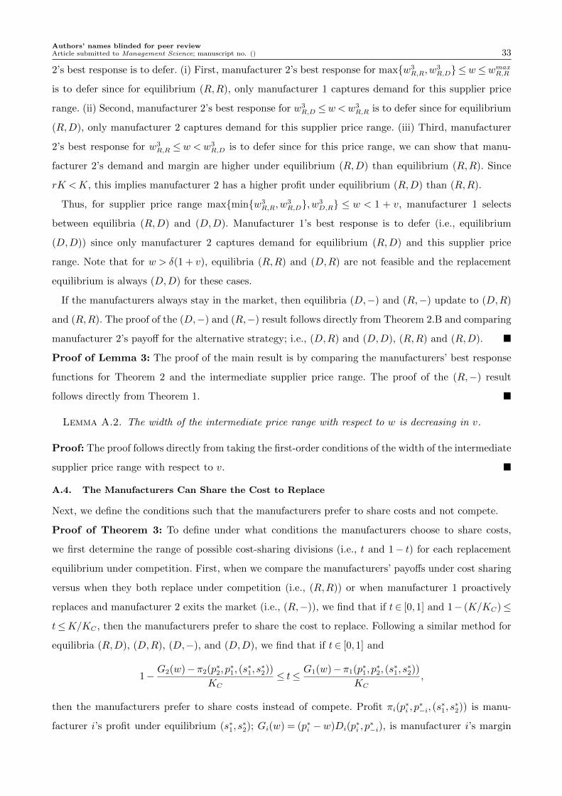
Authors’ names blinded for peer reviewArticle submitted to Management Science; manuscript no. () 33
2’s best response is to defer. (i) First, manufacturer 2’s best response for max{w3R,R,w
3R,D} ≤w≤wmaxR,R
is to defer since for equilibrium (R,R), only manufacturer 1 captures demand for this supplier price
range. (ii) Second, manufacturer 2’s best response for w3R,D ≤w<w3
R,R is to defer since for equilibrium
(R,D), only manufacturer 2 captures demand for this supplier price range. (iii) Third, manufacturer
2’s best response for w3R,R ≤ w <w3
R,D is to defer since for this price range, we can show that manu-
facturer 2’s demand and margin are higher under equilibrium (R,D) than equilibrium (R,R). Since
rK <K, this implies manufacturer 2 has a higher profit under equilibrium (R,D) than (R,R).
Thus, for supplier price range max{min{w3R,R,w
3R,D},w3
D,R} ≤ w < 1 + v, manufacturer 1 selects
between equilibria (R,D) and (D,D). Manufacturer 1’s best response is to defer (i.e., equilibrium
(D,D)) since only manufacturer 2 captures demand for equilibrium (R,D) and this supplier price
range. Note that for w > δ(1 + v), equilibria (R,R) and (D,R) are not feasible and the replacement
equilibrium is always (D,D) for these cases.
If the manufacturers always stay in the market, then equilibria (D,−) and (R,−) update to (D,R)
and (R,R). The proof of the (D,−) and (R,−) result follows directly from Theorem 2.B and comparing
manufacturer 2’s payoff for the alternative strategy; i.e., (D,R) and (D,D), (R,R) and (R,D). �
Proof of Lemma 3: The proof of the main result is by comparing the manufacturers’ best response
functions for Theorem 2 and the intermediate supplier price range. The proof of the (R,−) result
follows directly from Theorem 1. �
Lemma A.2. The width of the intermediate price range with respect to w is decreasing in v.
Proof: The proof follows directly from taking the first-order conditions of the width of the intermediate
supplier price range with respect to v. �
A.4. The Manufacturers Can Share the Cost to Replace
Next, we define the conditions such that the manufacturers prefer to share costs and not compete.
Proof of Theorem 3: To define under what conditions the manufacturers choose to share costs,
we first determine the range of possible cost-sharing divisions (i.e., t and 1− t) for each replacement
equilibrium under competition. First, when we compare the manufacturers’ payoffs under cost sharing
versus when they both replace under competition (i.e., (R,R)) or when manufacturer 1 proactively
replaces and manufacturer 2 exits the market (i.e., (R,−)), we find that if t∈ [0,1] and 1− (K/KC)≤
t≤K/KC , then the manufacturers prefer to share the cost to replace. Following a similar method for
equilibria (R,D), (D,R), (D,−), and (D,D), we find that if t∈ [0,1] and
1− G2(w)−π2(p∗2, p∗1, (s
∗1, s∗2))
KC
≤ t≤ G1(w)−π1(p∗1, p∗2, (s
∗1, s∗2))
KC
,
then the manufacturers prefer to share costs instead of compete. Profit πi(p∗i , p∗−i, (s
∗1, s∗2)) is manu-
facturer i’s profit under equilibrium (s∗1, s∗2); Gi(w) = (p∗i −w)Di(p
∗i , p∗−i), is manufacturer i’s margin
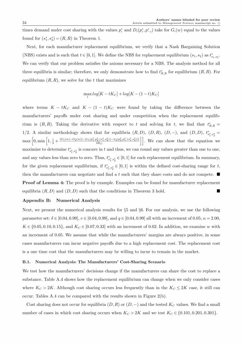
Authors’ names blinded for peer review34 Article submitted to Management Science; manuscript no. ()
times demand under cost sharing with the values p∗i and Di(p∗i , p∗−i) take for Gi(w) equal to the values
found for (s∗1, s∗2) = (R,R) in Theorem 1.
Next, for each manufacturer replacement equilibrium, we verify that a Nash Bargaining Solution
(NBS) exists and is such that t∈ [0,1]. We define the NBS for replacement equilibrium (s1, s2) as t∗s1,s2 .
We can verify that our problem satisfies the axioms necessary for a NBS. The analysis method for all
three equilibria is similar; therefore, we only demonstrate how to find t∗R,R for equilibrium (R,R). For
equilibrium (R,R), we solve for the t that maximizes
maxtlog[K − tKC ] + log[K − (1− t)KC ]
where terms K − tKC and K − (1 − t)KC were found by taking the difference between the
manufacturers’ payoffs under cost sharing and under competition when the replacement equilib-
rium is (R,R). Taking the derivative with respect to t and solving for t, we find that t∗R,R =
1/2. A similar methodology shows that for equilibria (R,D), (D,R), (D,−), and (D,D), t∗s∗1,s∗2=
max[0,min
[1, 1
2+
[G1(w)−G2(w)]−[π1(p∗1,p∗2,(s∗1,s∗2))−π2(p
∗2,p∗1,(s∗1,s∗2))]
2KC
]]. We can show that the equation we
maximize to determine t∗s∗1,s∗2is concave in t and thus, we can round any values greater than one to one,
and any values less than zero to zero. Thus, t∗s∗1,s∗2∈ [0,1] for each replacement equilibrium. In summary,
for the given replacement equilibrium, if t∗s∗1,s∗2∈ [0,1] is within the defined cost-sharing range for t,
then the manufacturers can negotiate and find a t such that they share costs and do not compete. �
Proof of Lemma 4: The proof is by example. Examples can be found for manufacturer replacement
equilibria (R,D) and (D,D) such that the conditions in Theorem 3 hold. �
Appendix B: Numerical Analysis
Next, we present the numerical analysis results for §5 and §6. For our analysis, we use the following
parameter set: δ ∈ [0.04,0.99], v ∈ [0.04,0.99], and q ∈ [0.04,0.99] all with an increment of 0.05; α= 2.00,
K ∈ {0.05,0.10,0.15}, and KC ∈ [0.07,0.33] with an increment of 0.02. In addition, we examine w with
an increment of 0.05. We assume that while the manufacturers’ margins are always positive, in some
cases manufacturers can incur negative payoffs due to a high replacement cost. The replacement cost
is a one time cost that the manufacturers may be willing to incur to remain in the market.
B.1. Numerical Analysis: The Manufacturers’ Cost-Sharing Scenario
We test how the manufacturers’ decisions change if the manufacturers can share the cost to replace a
substance. Table A.4 shows how the replacement equilibrium can change when we only consider cases
where KC > 2K. Although cost sharing occurs less frequently than in the KC ≤ 2K case, it still can
occur. Tables A.4 can be compared with the results shown in Figure 2(b).
Cost sharing does not occur for equilibria (D,R) or (D,−) and the tested KC values. We find a small
number of cases in which cost sharing occurs when KC > 2K and we test KC ∈ {0.101,0.201,0.301}.
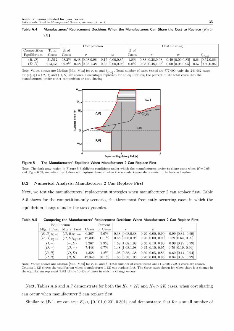
Authors’ names blinded for peer reviewArticle submitted to Management Science; manuscript no. () 35
Table A.4 Manufacturers’ Replacement Decisions When the Manufacturers Can Share the Cost to Replace (KC >
2K)
Competition Cost SharingCompetition Total % of % ofEquilibrium Cases Cases r w Cases r w t∗s∗1 ,s∗2
(R,D) 31,512 98.2% 0.48 [0.08,0.98] 0.15 [0.00,0.85] 1.8% 0.88 [0.28,0.98] 0.40 [0.00,0.85] 0.64 [0.52,0.86](D,D) 213,470 99.2% 0.48 [0.08,1.38] 0.35 [0.00,0.95] 0.8% 0.98 [0.48,1.38] 0.60 [0.05,0.95] 0.67 [0.50,0.96]
Note: Values shown are Median [Min, Max] for r, w, and t∗s∗1 ,s∗2
. Total number of cases tested are 777,000; only the 244,982 cases
for (s∗1 , s∗2) = (R,D) and (D,D) are shown. Percentages represent for an equilibrium, the percent of the total cases that the
manufacturers prefer either competition or cost sharing.
Sup
plie
r P
rice
(w
)
Expected Regulatory Risk (r)10 2
wH
wL
wmax
wD,D
(D,R)
(R,R)
(D,-)
(D,D)
(R,D)wR,D
Figure 5 The Manufacturers’ Equilibria When Manufacturer 2 Can Replace First
Note: The dark gray region in Figure 5 highlights conditions under which the manufacturers prefer to share costs when K = 0.05and KC = 0.09; manufacturer 2 does not capture demand when the manufacturers share costs in the hatched region.
B.2. Numerical Analysis: Manufacturer 2 Can Replace First
Next, we test the manufacturers’ replacement strategies when manufacturer 2 can replace first. Table
A.5 shows for the competition-only scenario, the three most frequently occurring cases in which the
equilibrium changes under the two dynamics.
Table A.5 Comparing the Manufacturers’ Replacement Decisions When Manufacturer 2 Can Replace First
Equilibrium PercentMfg. 1 First Mfg 2. First Cases of Cases r w δ
(R,D)D∗2=0 (D,R)D∗
1=0 6,267 5.6% 0.38 [0.08,0.88] 0.20 [0.00, 0.90] 0.99 [0.84, 0.99]
(R,D)D∗2=0 (R,D)D∗
2=0 12,305 11.1% 0.58 [0.08,0.98] 0.20 [0.00, 0.90] 0.89 [0.64, 0.99]
(D,−) (−,D) 3,267 2.9% 1.58 [1.08,1.98] 0.50 [0.10, 0.90] 0.99 [0.79, 0.99](D,−) (D,−) 7,448 6.7% 1.48 [1.08,1.98] 0.45 [0.10, 0.95] 0.79 [0.19, 0.99]
(R,R) (D,D) 1,358 1.2% 1.08 [0.88,1.38] 0.30 [0.05, 0.85] 0.69 [0.14, 0.94](R,R) (R,R) 42,346 38.1% 1.58 [0.38,1.98] 0.20 [0.00, 0.95] 0.84 [0.09, 0.99]
Note: Values shown are Median [Min, Max] for r, w, and δ. Total number of cases tested are 111,000; 72,991 cases are shown.Column 1 (2) shows the equilibrium when manufacturer 1 (2) can replace first. The three cases shown for when there is a change inthe equilibrium represent 9.8% of the 10.5% of cases in which a change occurs.
Next, Tables A.6 and A.7 demonstrate for both the KC ≤ 2K and KC > 2K cases, when cost sharing
can occur when manufacturer 2 can replace first.
Similar to §B.1, we can test KC ∈ {0.101,0.201,0.301} and demonstrate that for a small number of
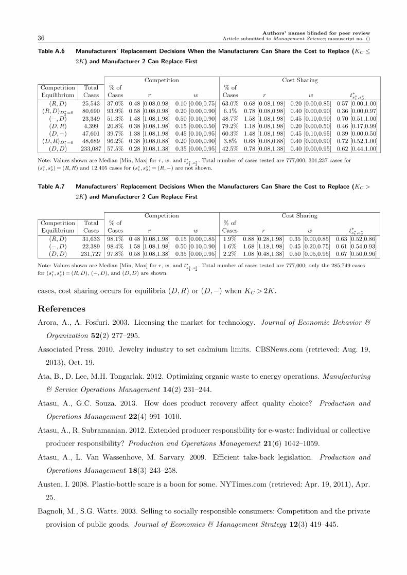
Authors’ names blinded for peer review36 Article submitted to Management Science; manuscript no. ()
Table A.6 Manufacturers’ Replacement Decisions When the Manufacturers Can Share the Cost to Replace (KC ≤2K) and Manufacturer 2 Can Replace First
Competition Cost SharingCompetition Total % of % ofEquilibrium Cases Cases r w Cases r w t∗s∗1 ,s∗2
(R,D) 25,543 37.0% 0.48 [0.08,0.98] 0.10 [0.00,0.75] 63.0% 0.68 [0.08,1.98] 0.20 [0.00,0.85] 0.57 [0.00,1.00](R,D)D∗
2=0 80,690 93.9% 0.58 [0.08,0.98] 0.20 [0.00,0.90] 6.1% 0.78 [0.08,0.98] 0.40 [0.00,0.90] 0.36 [0.00,0.97]
(−,D) 23,349 51.3% 1.48 [1.08,1.98] 0.50 [0.10,0.90] 48.7% 1.58 [1.08,1.98] 0.45 [0.10,0.90] 0.70 [0.51,1.00](D,R) 4,399 20.8% 0.38 [0.08,1.98] 0.15 [0.00,0.50] 79.2% 1.18 [0.08,1.98] 0.20 [0.00,0.50] 0.46 [0.17,0.99](D,−) 47,601 39.7% 1.38 [1.08,1.98] 0.45 [0.10,0.95] 60.3% 1.48 [1.08,1.98] 0.45 [0.10,0.95] 0.39 [0.00,0.50]
(D,R)D∗1=0 48,689 96.2% 0.38 [0.08,0.88] 0.20 [0.00,0.90] 3.8% 0.68 [0.08,0.88] 0.40 [0.00,0.90] 0.72 [0.52,1.00]
(D,D) 233,087 57.5% 0.28 [0.08,1.38] 0.35 [0.00,0.95] 42.5% 0.78 [0.08,1.38] 0.40 [0.00,0.95] 0.62 [0.44,1.00]
Note: Values shown are Median [Min, Max] for r, w, and t∗s∗1 ,s∗2
. Total number of cases tested are 777,000; 301,237 cases for
(s∗1 , s∗2) = (R,R) and 12,405 cases for (s∗1 , s
∗2) = (R,−) are not shown.
Table A.7 Manufacturers’ Replacement Decisions When the Manufacturers Can Share the Cost to Replace (KC >
2K) and Manufacturer 2 Can Replace First
Competition Cost SharingCompetition Total % of % ofEquilibrium Cases Cases r w Cases r w t∗s∗1 ,s∗2
(R,D) 31,633 98.1% 0.48 [0.08,1.98] 0.15 [0.00,0.85] 1.9% 0.88 [0.28,1.98] 0.35 [0.00,0.85] 0.63 [0.52,0.86](−,D) 22,389 98.4% 1.58 [1.08,1.98] 0.50 [0.10,0.90] 1.6% 1.68 [1.18,1.98] 0.45 [0.20,0.75] 0.61 [0.54,0.93](D,D) 231,727 97.8% 0.58 [0.08,1.38] 0.35 [0.00,0.95] 2.2% 1.08 [0.48,1.38] 0.50 [0.05,0.95] 0.67 [0.50,0.96]
Note: Values shown are Median [Min, Max] for r, w, and t∗s∗1 ,s∗2
. Total number of cases tested are 777,000; only the 285,749 cases
for (s∗1 , s∗2) = (R,D), (−,D), and (D,D) are shown.
cases, cost sharing occurs for equilibria (D,R) or (D,−) when KC > 2K.
References
Arora, A., A. Fosfuri. 2003. Licensing the market for technology. Journal of Economic Behavior &
Organization 52(2) 277–295.
Associated Press. 2010. Jewelry industry to set cadmium limits. CBSNews.com (retrieved: Aug. 19,
2013), Oct. 19.
Ata, B., D. Lee, M.H. Tongarlak. 2012. Optimizing organic waste to energy operations. Manufacturing
& Service Operations Management 14(2) 231–244.
Atasu, A., G.C. Souza. 2013. How does product recovery affect quality choice? Production and
Operations Management 22(4) 991–1010.
Atasu, A., R. Subramanian. 2012. Extended producer responsibility for e-waste: Individual or collective
producer responsibility? Production and Operations Management 21(6) 1042–1059.
Atasu, A., L. Van Wassenhove, M. Sarvary. 2009. Efficient take-back legislation. Production and
Operations Management 18(3) 243–258.
Austen, I. 2008. Plastic-bottle scare is a boon for some. NYTimes.com (retrieved: Apr. 19, 2011), Apr.
25.
Bagnoli, M., S.G. Watts. 2003. Selling to socially responsible consumers: Competition and the private
provision of public goods. Journal of Economics & Management Strategy 12(3) 419–445.
Authors’ names blinded for peer reviewArticle submitted to Management Science; manuscript no. () 37
Bailin, P.S., M. Byrne, S. Lewis, R. Liroff. 2008. Public awareness drives market for safer alternatives.
www.iehn.org (retrieved: Sept. 23, 2013), Sept. 15.
Baker, E., E. Shittu. 2006. Profit-maximizing R&D in response to a random carbon tax. Resource and
Energy Economics 28(2) 160–180.
Bakshi, N., P. Kleindorder. 2009. Co-opetition and investment for supply-chain resilence. Product and
Operations Management 18(6) 583–603.
Bhaskaran, S.R., V. Krishnan. 2009. Effort, revenue, and cost sharing mechanisms for collaborative
new product development. Management Science 55(7) 1152–1169.
BIFMA. 2014. Business and Institutional Furniture Manufacturers Association: Furniture Sustainabil-
ity Standard. www.bifma.org (retrieved: July 17, 2014).
Brody, J. 1983. Personal health: Judging safety of aspartame in soft drinks. NYTimes.com (retrieved:
Apr. 21, 2008), July 13.
Callahan, P., S. Roe. 2012. Fear fans flames for chemical makers. ChicagoTribune.com (retrieved: May
6, 2012), May 6.
Carbone, J. 2008. RoHS cost: $32 billion and counting. Purchasing.com (retrieved: Sept. 21, 2009),
June 12.
Caro, F., C.J. Corbett, T. Tan, R. Zuidwijk. 2013. Double counting in supply chain carbon footprinting.
Manufacturing and Service Operations Management 15(4) 545–558.
Carter, C.R., J.R. Carter. 1998. Interorganizational determinants of environmental purchasing: Initial
evidence from the consumer products industries. Decision Sciences 29(3) 659–684.
ChemSec. 2009. Dell: The SIN List provides advance warning of restrictions to come. www.chemsec.org
(retrieved: Oct. 2, 2010), Oct. 15.
Consumer Reports. 1999. Baby alert: New findings about plastics. GreenerChoices.org (retrieved: Aug.
24, 2014), May.
Coolidge, A. 2013. P&G halts use of 2 chemicals in personal care products. Cincinnati.com (retrieved:
Sept. 7, 2013), Sept. 6.
Corbett, C.J., G.A. DeCroix. 2001. Shared-savings contracts for indirect materials supply chains:
Channel profits and environmental impacts. Management Science 47(7) 881–893.
Cortazar, G., E. Schwartz, M. Salinas. 1998. Evaluating environmental investments: A real options
approach. Management Science 44(8) 1059–1070.
D’Aspremont, C., A. Jacquemin. 1988. Cooperative and noncooperative R&D in duopoly with
spillovers. The American Economic Review 78(5) 1133–1137.
Drake, D., P.R. Kleindorfer, L.N. Van Wassenhove. 2012. Technology choice and capacity portfolios
under emissions regulation. Working paper, Harvard Business School, Boston, MA.
Elias, A., T. Kraft, G. Raz. 2013. Eastman Tritan. Darden Business Publishing UVA–OM–1494.
Authors’ names blinded for peer review38 Article submitted to Management Science; manuscript no. ()
Ewell, J. 2013. Interview by the authors. Sustainable Materials Director, GreenBlue, August 29.
Fahmy, D. 2010. Chemicals in toys, furniture may face tighter standards. ABCNews.com (retrieved:
Sept. 6, 2013), Feb. 22.
Farzin, Y.H., P.M. Kort. 2000. Pollution abatement investment when environmental regulation is
uncertain. Journal of Public Economic Theory 2(2) 183–212.
Fudenberg, D., J. Tirole. 1985. Preemption and rent equalization in the adoption of new technology.
Review of Economic Studies 52(3) 383–401.
Gaimon, C. 1989. Dynamic game results of the acquisition of new technology. Operations Research
37(3) 410–425.
Geffen, C.A., S. Rothenberg. 2000. Suppliers and environmental innovation. Journal of Operations
and Production Management 20(2) 166–186.
Goyal, M., S. Netessine. 2007. Strategic technology choice and capacity investment under demand
uncertainty. Management Science 53(2) 192–207.
Grady, D. 2010. In feast of data on BPA plastic, no final answer. NYTimes.com (retrieved: Sept. 26,
2010), Sept. 6.
Hagedoorn, J., J. Schakenraad. 1994. The effect of strategic technology alliances on company perfor-
mance. Strategic Management Journal 15(4) 291–309.
Halliday, J. 2008. Gap is closing on aspartames lead over sucralose: Mintel data.
www.foodnavigator.com (retrieved: Feb. 18, 2010), July 24.
Hamel, G. 1991. Competition for competence and inter-partner learning within international strategic
alliances. Strategic Management Journal 12(S1) 83–103.
Hannan, T.H., J.M. McDowell. 1984. The determinants of technology adoption: The case of the banking
firm. RAND Journal of Economics 15(3) 328–335.
Hartl, R.F. 1992. Optimal acquisition of pollution control equipment under uncertainty. Management
Science 38(5) 609–622.
Hoppe, H.C. 2000. Second-mover advantages in the strategic adoption of new technology under uncer-
tainty. International Journal of Industrial Organization 18(2) 315–338.
Huisman, J.M., P.M. Kort. 2004. Strategic technology adoption taking into account future technological
improvements: A real options approach. European Journal of Operational Research 159(3) 705–728.
Isik, M. 2004. Incentives for technology adoption under environmental policy uncertainty: Implications
for green payment programs. Environmental and Resource Economics 27(3) 247–263.
Jacobs, B., R. Subramanian. 2011. Sharing responsibility for product recovery across the supply chain.
Production and Operations Management 21(1) 85–100.
Jap, S.D. 2001. “Pie sharing” in complex collaboration contexts. Journal of marketing research 38(1)
86–99.
Authors’ names blinded for peer reviewArticle submitted to Management Science; manuscript no. () 39
Jensen, R. 1982. Adoption and diffusion of an innovation of uncertain profitability. Journal of Economic
Theory 27(1) 182–193.
Kamien, M.I., Y. Tauman. 1984. The private value of a patent: A game theoretic analysis. Journal of
Economics 4 93–118.
Kary, T. 2014. Colgate Total ingredient linked to hormones, cancer spotlights FDA process.
Bloomberg.com (retrieved: Aug. 14, 2014), Aug. 11.
Katz, M.L., C. Shapiro. 1986. Technology adoption in the presence of network externalities. The
Journal of Political Economy 94(4) 822–841.
Klassen, R. 2000. Exploring the linkage between investment in manufacturing and environmental
technologies. International Journal of Operations & Production Management 20(2) 127–147.
Koch, W. 2013. Wal-Mart announces phase-out of hazardous chemicals. USAToday.com (retrieved:
Sept. 13, 2013), Sept. 12.
Kraft, T., F. Erhun, R. Carlson, D. Rafinejad. 2013a. Replacement decisions for potentially hazardous
substances. Production and Operations Management 22(4) 958–975.
Kraft, T., Y. Zheng, F. Erhun. 2013b. The NGO’s dilemma: How to influence firms to replace a
potentially hazardous substance. Manufacturing and Service Operations Management 15(4) 649–
669.
Krass, D., T. Nedorezov, A. Ovchinnikov. 2013. Environmental taxes and the choice of green technol-
ogy. Production & Operations Management. Forthcoming.
Kroes, J., R. Subramanian, R. Subramanyam. 2012. Operational compliance levers, environmental
performance, and firm performance under cap and trade regulation. Manufacturing and Service
Operations Management 14(2) 186–201.
Krysiak, F.C. 2008. Price vs. quantities: The effects on technology choice. Journal of Public Economics
92(5) 1275–1287.
Kuchment, A. 2008. The baby bottle blues. Newsweek 53 Jan. 14.
Kurtulus, M., S. Ulku, B.L. Toktay. 2012. The value of collaborative forecasting in supply chains.
Manufacturing and Service Operations Management 14(1) 82–98.
Lado, A.A., N.G. Boyd, S.C. Hanlon. 1997. Competition, cooperation, and the search for economic
rents: A syncretic model. Academy of Management Review 22(4) 110–141.
Layton, L. 2009. No BPA for baby bottles in U.S. WashingtonPost.com (retrieved: Sept. 14, 2009),
Mar. 6.
Lee, S.M. 2013. Law advising public of chemical dangers kicking in. SFGate.com (retrieved: Sept. 28,
2013), Sept. 27.
Levin, S.G., S.L. Levin, J.B. Meisel. 1987. A dynamic analysis of the adoption of a new technology:
The case of optical scanners. The Review of Economics and Statistics 12–17.
Authors’ names blinded for peer review40 Article submitted to Management Science; manuscript no. ()
Majumder, P., H. Groenevelt. 2001. Competition in remanufacturing. Production and Operations
Management 10(2) 125–141.
Mamer, J.W., K.F. McCardle. 1987. Uncertainty, competition, and the adoption of new technology.
Management Science 33(2) 161–177.
Maxwell, J.W., C.S. Decker. 2006. Voluntary environmental investment and responsive regulation.
Environmental & Resource Economics 33(4) 425–439.
Moorthy, K.S. 1988. Product and price competition in a duopoly. Marketing Science 7(2) 141–165.
Mui, Y. 2008. Wal-Mart to pull bottles made with chemical BPA. WashingtonPost.com (retrieved:
Feb. 14, 2009), Apr. 18.
Nagarajan, M., G. Sosic. 2008. Game-theoretic analysis of cooperation among supply chain agents:
Review and extensions. European Journal of Operations Research 187(3) 719–745.
Nidumolu, R., J. Ellison, J. Whalen, E. Billman. 2014. The collaboration imperative. Harvard Business
Review (April) 76–84.
Orsdemir, A., E. Kemahlioglu-Ziya, A.K. Parlakturk. 2014. Competitive quality choice and remanu-
facturing. Production and Operations Management 23(1) 48–64.
Plambeck, E., Q. Wang. 2009. Effects of e-waste regulation on new product introduction. Management
Science 55(3) 333–347.
Plambeck, E.L., T.A. Taylor. 2005. Sell the plant? The impact of contract manufacturing on innovation,
capacity, and profitability. Management Science 51(1) 133–155.
Pous, T. 2012. “Toxic threads” study finds high levels of dangerous chemicals in popular brands.
Time.com (retrieved: Dec. 12, 2012), Nov. 21.
Raz, G., C. Druehl, V. Blass. 2013. Design for the environment Life cycle approach using a newsvendor
model. Production and Operations Management 22(4) 940–957.
Reinganum, J.F. 1981. On the diffusion of new technology: A game theoretic approach. The Review
of Economic Studies 48(3) 395–405.
Requate, T. 2005. Timing and commitment of environmental policy, adoption of new technology, and
repercussions on R&D. Environmental and Resource Economics 31(2) 175–199.
Rizzuto, P. 2013. TSCA reform bill seen as promising but road to enactment is uncertain. BNA.com
(retrieved: Sept. 6, 2013), June 3.
Shan, W. 1990. An empirical analysis of organizational strategies by entrepreneurial high-technology
firms. Strategic Management Journal 11(2) 129–139.
Shy, O. 1995. Industrial organization: Theory and applications. MIT Press, Cambridge, MA.
Singh, N., X. Vives. 1984. Price and quantity competition in a differentiated duopoly. RAND Journal
of Economics 15(4) 546–554.
Authors’ names blinded for peer reviewArticle submitted to Management Science; manuscript no. () 41
Tarui, N., S. Polasky. 2005. Environmental regulation with technology adoption, learning and strategic
behavior. Journal of Environmental Economics and Management 50(3) 447–467.
Tavernise, S. 2012. F.D.A. makes it official: BPA can’t be used in baby bottles and cups. NYTimes.com
(retrieved: July 17, 2012), July 17.
The SIN List. 2014. The SIN (Substitute It Now!) List. www.chemsec.org (retrieved: Aug. 14, 2014).
Toyasaki, F., T. Boyaci, V. Verter. 2010. An analysis of monopolistic and competitive take-back
schemes for WEEE recycling. Production and Operations Management 20(6) 805–823.
Vachon, S., R.D. Klassen. 2008. Environmental management and manufacturing performance: The
role of collaboration in the supply chain. International Journal of Production Economics 11(2)
299–315.
Wang, E.T.G., A. Seidmann. 1995. Electronic data interchange: Competitive externalities and strategic
implementation policies. Management Science 41(3) 401–418.
Yalabik, B., R.J. Fairchild. 2011. Customer, regulatory, and competitive pressure as drivers of envi-
ronmental innovation. International Journal of Production Economics 131(2) 519–527.