Embed Size (px)
Citation preview

Improvement of EDR forecast by consideration of horizontal shear and SSO wake production using
the concept of scale separation:
Matthias Raschendorfer, FE 14
COSMO user seminar Offenbach: 09-11.03.2009Matthias Raschendorfer
DWD-Project:
Improvement of turbulence forecast for civil aviation
Eddy Dissipation Rate

Motivation:
Turbulence has major impacts on aviation:
Impacts of turbulenceTurbulence has major impacts on aviation. According to a review of National Traffic Safety Board data from 1992 to 2001 by the National Aviation Safety Data Analysis Center, turbulence was a factor in at least 509 accidents in the United States, including 251 deaths (mostly in the general aviation sector). Additionally, the FAA Joint Safety Analysis Team estimated that there are more than 1,000 minor turbulence-related injuries on commercial aircraft annually. Airlines lose millions of dollars every year due to turbulence because of injury claims, delays, extra fuel costs, and aircraft damage.
NCAR News Release
NCAR Teams with United Airlines to Pinpoint Turbulence in Clouds;Research Can Help Reduce Delays, Injuries, CostsSeptember 6, 2007
COSMO user seminar Offenbach: 09-11.03.2009Matthias Raschendorfer

( )k32EDR 3
2
lnln ⋅−⎟⎟⎠
⎞⎜⎜⎝
⎛⋅α
turbulent peak wavelength
ln [wave number k]
( )[ ]( )aircraftoffunctionnattenuatio
TKEofdensityspectralklnln
+⋅
( )Vfln
frequency of aircraft oscillations
aircraft velocity with respect to mean wind
TKECKE
model resolution
turbulence
attenuation functionand velocity
of the aircraft
spectrum of vertical oscillations
inertial sub range spectrum of atmosphere
EDR by regression of the Kolmogorov spectrum
Aircraft measurements of EDR:( )[ ]energywindofdensityspectralk ⋅ln
COSMO user seminar Offenbach: 09-11.03.2009Matthias Raschendorfer

Turbulence index = 1 (light) Turbulence index = 4 (moderate)
Turbulence index = 5 (severe)Colours for measurement height in [m]
COSMO user seminar Offenbach: 09-11.03.2009Matthias Raschendorfer
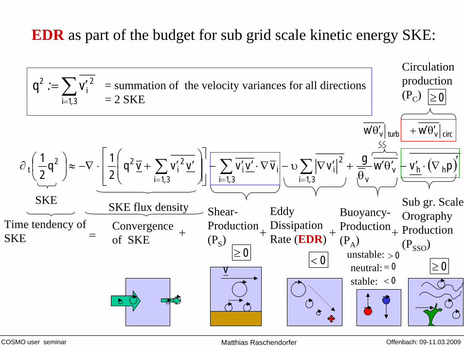
EDR as part of the budget for sub grid scale kinetic energy SKE:
∑=
′=31i
2i
2 vq,
: = summation of the velocity variances for all directions
( )′∇⋅′−θ′′θ
+′∇υ−∇⋅′′−⎥⎥⎦
⎤
⎢⎢⎣
⎡⎟⎟⎠
⎞⎜⎜⎝
⎛′′+⋅−∇≈⎟
⎠⎞
⎜⎝⎛∂ ∑∑∑
===
pvwgvvvvvvvq21q
21
hhvv31i
2ii
31ii
31i
2i
22t
,,,
SKE SKE flux density Shear-Production (PS)
Buoyancy-Production (PA)
Eddy DissipationRate (EDR)
Sub gr. Scale Orography Production (PSSO)
0≥ 0< 0≥unstable:neutral:stable: 0<
0>0=
Time tendency of SKE +Convergence
of SKE= + ++
= 2 SKE
v
COSMO user seminar Offenbach: 09-11.03.2009Matthias Raschendorfer
circvturbv ww θ′′+θ′′
Circulation production (PC) 0≥

Turbulence closure on level 2.5 (according to MY):
• We solve the system of reduced second order equations (after substituting the turbulent stress tensor by its traceless form)
using special closure assumptions in order to express the unknown statistical moments in those equations
• They are in accordance only with a special class of sub grid scale structures that we call turbulence (stochastic isotropic)
- In particular we neglect all transport terms and time tendency terms
- but we use a
- closure of pressure correlation and dissipation terms according to Rotta and Kolmogorov using a turbulent length scale according to Blackadar
yielding in particular:lEDR
3qEDRα
−≈
All reduced second order budgets degenerate to a system of linear equations
prognostic equation for turbulent SKE (TKE)
l
COSMO user seminar Offenbach: 09-11.03.2009Matthias Raschendorfer
• Neglect of all horizontal gradients (BLA) in the second order budgets:The only relevant vertical flux densities have got flux gradient form
COSMO user seminar Offenbach: 09-11.03.2009Matthias Raschendorfer

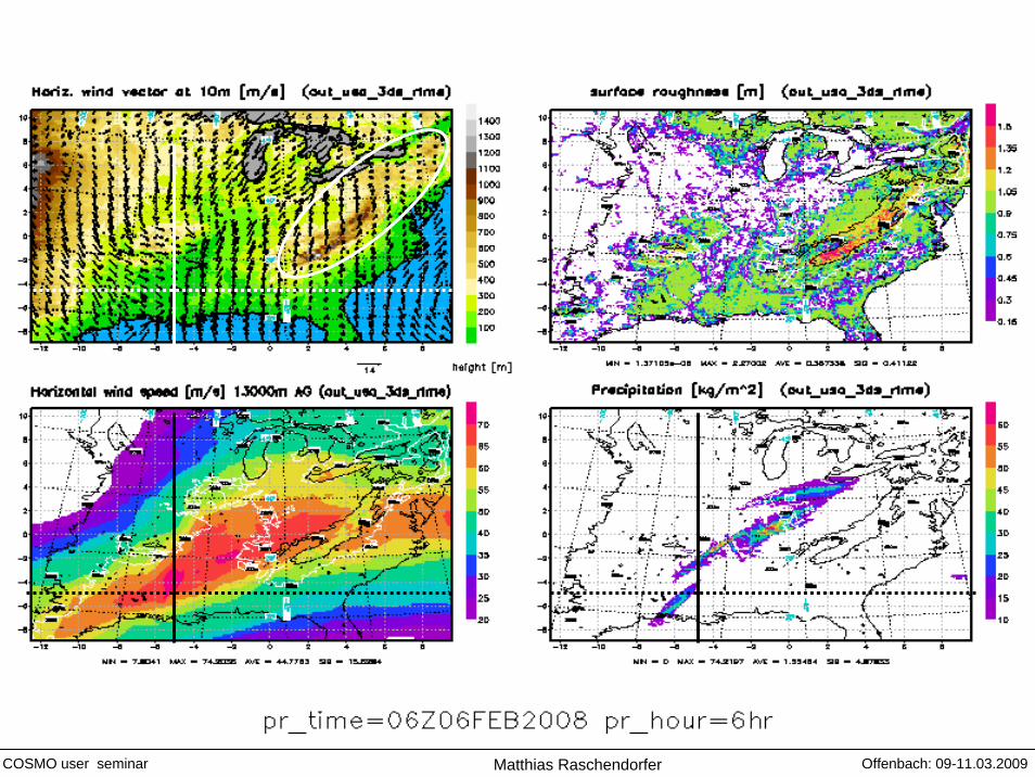
Cross section of model output over the chosen USA domain
from North to South cutting the jet stream
Turbulenzvorhersage für die Luftfahrt Matthias Raschendorfer 16.04.2008
Horizontal wind speed [m/s] Eddy dissipation parameter [m2/3/s]
06.02.2008 00UTC + 12h -90 E
moderate light
S N S N
Appalachian mountains
Jetstream
scale interaction by (positive definite circulation term)
Physical based solutionalso above the BL

EDR from turbulence model
- improved by consideration of horizontal shearand related length scales as an additional TKE production
- Improved by considering the interactions between turbulence and mountain blocking
- Improvement by considering the interactions between turbulence and convection
Other proper turbulence indicators, like- Ri-number, vertical gradients of temperature und wind- Horizontal shear- large scale surface roughness- …
regression model EDR from aircraft
measurements
( ) mesaa EDRScherungZahlRiEDRfn1
≈KK ,,_,mod,,
Aim of the DWD-Project:
COSMO user seminar Offenbach: 09-11.03.2009Matthias Raschendorfer

( )∑∑==
∂⋅∂+∂⋅≈∇⋅′′−=3
1jijijiij
M3
1iiiS vvvKvvvP
,:
( )jiijM
ji vvKvv ∂+∂⋅−≈′′
3D-shear production for turbulent-isotropic structures:
isotropic-turbulent contribution to the stress tensor
l⋅⋅= MM SqK isotropic-turbulent diffusion coefficient
Isotropic-turbulent 3D shear term:
( ) ( )22z2
1zHBA vv ∂+∂⎯⎯→⎯
( ) ( ) ( )( ) ( ) ( )[ ]2
332
222
11
22332
21331
21221
vvv2
vvvvvv
∂+∂+∂+
∂+∂+∂+∂+∂+∂
COSMO user seminar Offenbach: 09-11.03.2009Matthias Raschendorfer

m9000≈COSMO user seminar Offenbach: 09-11.03.2009Matthias Raschendorfer

horizontal grid scale
z
pL
Prandtl-layer
roughness layer
Eckmann-layer
height of the troposphere
boundary layer height
Blackadar
HD0
Separated horizontal shear mode:
Offenbach: 09-11.03.2009Matthias RaschendorferCOSMO user seminar

( ) ( ) ( )[ ]222
211
21221HHHSH vv2vvDqP ∂+∂+∂+∂⋅β⋅=:
Separated horizontal shear term:
effective mixing length of diffusion by separated horizontal shear eddies:
velocity scale of separated horizontal shear eddies
1H <β related scaling parameter
Equilibrium with scale transfer towards the turbulence mode:
HH
3HM
HHHH DqFDq
α=⋅β⋅
MHF:=
1H <α scaling parameter similar to
23
MH
2H
23
H21
HMHHHHSH FDFDqP ⋅βα=⋅β=
2Sα=:
EDRα
COSMO user seminar Offenbach: 09-11.03.2009Matthias Raschendorfer
effective scaling parameter
Parameterization of the separated horizontal shear mode:

out_usa_shs_rlme_a_shsr_0.2
out_usa_shs_rlme_a_shsr_0.2
m9000≈COSMO user seminar Offenbach: 09-11.03.2009Matthias Raschendorfer

out_usa_shs_rlme_a_shsr_0.2
20
40
60
Pot. Temperature [K]
S N
COSMO user seminar Offenbach: 09-11.03.2009Matthias Raschendorfer

The wake production term:
( ) ( )[ ] ( )∫∈
′−∂−ρ−∇υ−′′+ρ⋅−∇=ρ∂B
2iiiiiit sdnp
G1pgvvvvvv
ss
Filtered momentum budget:
B
Q∂
n
ivSSOQ blocking
In the TKE-budget:
( ) ( ) ∑∫=∈
⋅−=′⋅≈′∇⋅′−≈2
1i
vSSOi
B
2h
hhhSSO
iQvsdnpGv
pvPs
s
hv
21x ,
3x
COSMO user seminar Offenbach: 09-11.03.2009Matthias Raschendorfer

out_usa_shs_rlme_a_shsr_0.2
out_usa_shs_rlme_a_shsr_0.2
m350≈
out_usa_shs_sso_turb_rlme_sso
out_usa_shs_sso_turb_rlme_sso
COSMO user seminar Offenbach: 09-11.03.2009Matthias Raschendorfer

10X10 GP above Appalachian mountains
out_usa_shs_rlme_ssoout_usa_shs_rlme_a_shsr_0.2
COSMO user seminar Offenbach: 09-11.03.2009Matthias Raschendorfer

• 3D-shear terms have got a significant effect only, when formulated as a scale interaction term producing TKE by shear of a separated horizontal shear mode with its own length scale
• Wake production of TKE by blocking can be formulated as a scale interaction termas well and can be described by scalar multiplication of the horizontal wind vectorwith its SS0-tendencies yielding some effect above mountainous terrain.
Conclusion:
• Next we plan to introduce a vertically resolved roughness layer including a more sophisticated interaction between turbulence and topographic blocking.
Prospect:
• We intent to derive a similar scale interaction term from the convection scheme as well.
COSMO user seminar Offenbach: 09-11.03.2009Matthias Raschendorfer

COSMO user seminar Offenbach: 09-11.03.2009Matthias Raschendorfer
Thanks for your attention!

Second order closure for the unknown statistical moments:
2-nd order budgets in TA:
( ) ( ) ( ) ( ) ( )( )( ) φψψφ
ψφ
ψφφφ
+φ′′+ψ′′+
φ∇⋅+ψ∇⋅+
φ∇⋅′′ψ′′ρ+ψ∇⋅′′φ′′ρ−φ∇⋅+ψ∇⋅−=φ′′+ψ′′+′′ψ′′φ′′ρ+ψ′′φ′′ρ⋅∇+ψ′′φ′′ρ∂=ψ′′φ′′ρ
prs
tt
QQQ
eeD
ee
vveevv ˆ~ˆ~ˆ~ˆ~~~~ˆ:
neglected outside the laminar layer
shear production
molecular dissipation
sub grid scale macroscopic transport
( )( ) φ∂′∂′+φ ′′∂′+
∂′∂φ ′′+∂φ ′′−
′φ ′′∂−
σ
σ
ˆzii
zii
i
zpp
pzp
p
⎭⎬⎫
⎩⎨⎧
=ψ∂ψ ′′−∈ψ
+⎭⎬⎫
⎩⎨⎧
=φ∂φ ′′−∈φ
jjii vp0
vp0
,H,
,H,
φ∇−= φφ a:emolecular flux density phase change production
pressure transport
pressure destruction
buoyancy source≈θ′′φ ′′ρθ v
v
gˆ
Projekt: „Turbulenzvorhersage für die Luftfahrt“ Offenbach: 17.04.2008Matthias Raschendorfer

Solution in horizontal boundary layer approximation:
• Neglect of all horizontal gradients in the second order budgets:
The only relevant vertical flux densities have got flux gradient form:
φ∂⋅−=′φ′ φzKw
l⋅⎭⎬⎫
⎩⎨⎧⋅=φ
M
H
SSqK turbulent diffusion coefficient for
vertical shear production( )2zu uKSP ∂⋅=
vzv
gKAP θ∂θ⋅−= θ
scalars
momentum
stability function dependent on and
buoyant production
( )2zu∂ vzv
gθ∂
θ
TKE2 ⋅ turbulent length scale
( )2zM
vzH
v uSSg
SPAPRi
∂θ∂
θ=−=:
Richardson-number
COSMO user seminar Offenbach: 09-11.03.2009Matthias Raschendorfer

Neglect of ( )ψ ′′φ ′′ρtD , in particular all transport terms (equilibrium) except in the SKE equation
Neglect of sub grid scale phase change production ( )ψφ φ ′′+ψ ′′ QQ
Neglect of pressure transport pi ′φ ′′∂−
Bernoulli approximation constgz2
pptot ≈ρ+⋅
ρ+=vv:
Confluence/diffluence model of local isotropy for a single mode of wave length kL : ( )k
jjj
vv
l
φ ′′⋅′′≈″φ∂⋅′′
φ′′
jx
jv ′′
kl0 kL
1. Primary turbulent closure assumptions:
1x
2x3x
What is the idea of turbulence closure?
Projekt: „Turbulenzvorhersage für die Luftfahrt“ Offenbach: 17.04.2008Matthias Raschendorfer

2. Secondary turbulent closure assumptions:
- spectral density of contributing modes follows a power law in terms of wave length in each direction:
- whole spectrum in a given direction is determined by a single peak wave length
- the peak wave length is the same for samples in all directions: isotropic length scale
- pressure correlation and dissipation can be closed using a single turbulent master length scalefor each location
inertial sub range spectrum
Turbulence is that class of sub grid scale structures being in agreement with turbulence closure assumptions!
Projekt: „Turbulenzvorhersage für die Luftfahrt“ Offenbach: 17.04.2008Matthias Raschendorfer
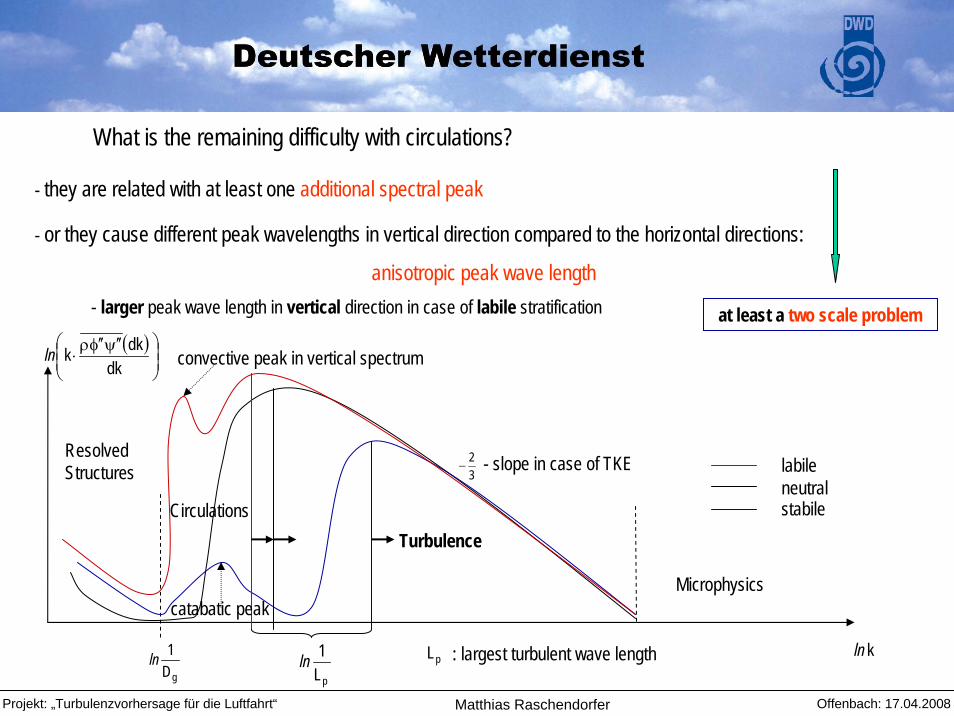
What is the remaining difficulty with circulations?
- they are related with at least one additional spectral peak
- or they cause different peak wavelengths in vertical direction compared to the horizontal directions:
anisotropic peak wave length- larger peak wave length in vertical direction in case of labile stratification
kln
( )⎟⎟⎠
⎞⎜⎜⎝
⎛ ψ ′′φ ′′ρ⋅
dkdkkln
32
− - slope in case of TKE
gD1ln
TurbulenceCirculations
Microphysics
ResolvedStructures
pL : largest turbulent wave length
convective peak in vertical spectrum
catabatic peak
neutralstabile
labile
pL1ln
at least a two scale problem
Projekt: „Turbulenzvorhersage für die Luftfahrt“ Offenbach: 17.04.2008Matthias Raschendorfer