Efficient Trajectory Optimization for Robot Motion Planning

Yu Zhao, Hsien-Chung Lin, and Masayoshi Tomizuka

Abstract— Motion planning for multi-jointed robots is chal-lenging. Due to the inherent complexity of the problem, mostexisting works decompose motion planning as easier subprob-lems. However, because of the inconsistent performance metrics,only sub-optimal solution can be found by decomposition basedapproaches. This paper presents an optimal control basedapproach to address the path planning and trajectory planningsubproblems simultaneously. Unlike similar works which eitherignore robot dynamics or require long computation time, anefficient numerical method for trajectory optimization is pre-sented in this paper for motion planning involving complicatedrobot dynamics. The efficiency and effectiveness of the proposedapproach is shown by numerical results. Experimental resultsare used to show the feasibility of the presented planningalgorithm.

I. INTRODUCTION

Motion planning for robots with multi-jointed arms is

challenging. Due to the complicated geometric structure and

nonlinear dynamics, time-consuming computation is required

to solve motion planning problem even in the simplest cases.

Most existing works utilize the path-velocity decomposition

approach [1], in which motion planning problem is separated

into easier subproblems, i.e., path planning and trajectory

planning. The path planning problem focuses on the gener-

ation of collision free geometric path in the configuration

space, while the trajectory planning problem focuses on

the generation of time optimal velocity profile along the

geometric path. Extensive research [2], [3], [4], [5] has been

conducted for each subproblem, resulting a rich collection

of algorithms. However, due to the inconsistency of perfor-

mance metrics between motion planning problem and the

subproblems, only sub-optimal solution can be found by

path-velocity decomposition based approaches. Time optimal

motion planning involving collision avoidance requirement

and robot dynamics is still a challenging problem ([6], [7]).

In order to avoid the inconsistency of performance metrics,

this paper presents an optimal control based approach to

address the path planning and trajectory planning problems

simultaneously. The presented approach is able to generate

time optimal trajectories without predetermining the geomet-

ric path while satisfying constraints involving robot dynam-

ics. Similar works can be found in [8], [9], [10]. However

either robot dynamics are ignored or long computation time

is required in these works. In this paper, an efficient numer-

ical method for trajectory optimization is utilized to solve

the optimal control problem for robot motion planning. It is

Yu Zhao, Hsien-Chung Lin, and Masayoshi Tomizuka are with the De-partment of Mechanical Engineering, University of California at Berkeley,Berkely, CA 94720, USA {yzhao334,hclin}@berkeley.edu,tomizuka@me.berkeley.edu

shown by numerical results that the solution can be found

with short computation time even when complicated robot

dynamics are involved. Experimental results have shown the

feasibility of the planned motion.

The rest part of this paper is organized as follows: section

II presents optimal control formulation for robot motion

planning problems, section III presents an efficient numerical

method for trajectory optimization, section IV presents nu-

merical and experimental results of the proposed approach,

and section V concludes this paper.

II. PROBLEM FORMULATION

A general optimal control problem can be posed as fol-

lows: determine the state-control function pair, t 7→ (xxx,uuu),terminal time tf , that minimize the performance metric or

cost function, while satisfying dynamic constraints, path con-

straints, and boundary conditions ([11]). The robot motion

planning problem can be formulated as an optimal control

problem by defining the cost function, dynamic constraints,

path constraints, and boundary conditions.

The state and control in motion planning involving robot

dynamics can be defined as:

xxx(t) =

[

qqq(t)qqq(t)

]

, uuu(t) = τττ(t) (1)

where t ∈ [0, tf ], qqq(t) = [q1(t), · · · , qn(t)]T

is the vector for

joint positions, and τττ(t) = [τ1(t), · · · , τn(t)]T

is the vector

for joint torques, n is the number of robot joints.

A. Cost Function

The quality of the planned motion strongly depends on

the formulation of cost function. In this paper, the cost

function is formulated as a summation of motion time tfand a regularization term for smoothness and naturalness of

the generated motion:

J = tf + µ

∫ tf

0

...qqq (t)TQQQ

...qqq (t)dt (2)

where...qqq (t) is the jerk of joint motion. The regularization

term is designed based on the minimum-jerk model of human

motion ([12]) and thus corresponds to the importance of the

naturalness of the generated motion. µ ≥ 0 is a weighting

coefficient for the regulation term, and QQQ is a weight matrix

designed to penalize the motion of joints with higher gear

ratios. The weight matrix QQQ is defined as

QQQ(i, j) =

{

0, j 6= i

1/

RRR(i, i)2 , j = i(3)

The case µ = 0 corresponds to the time optimal motion

planning problem. Larger µ slows down the generated mo-

tion, but increases the naturalness and smoothness.

B. Dynamic Constraints

The dynamic constraints is the robot dynamics. The equa-

tions of motion can be derived using Lagrangian’s equations

or Newton-Euler approach:

MMM(qqq)qqq +CCC(qqq, qqq)qqq +GGG(qqq) + ffff = τττ (4)

where MMM(qqq) ∈ Rn×n is the inertia matrix, CCC(qqq, qqq)qqq ∈ R

n×1

is the Coriolis and centrifugal force term, GGG(qqq) ∈ Rn×1 is

the gravity term, and ffff ∈ Rn×1 is the friction term. For

multi-jointed robot arms, all of these terms are inherently

nonlinear.

Letting xxx1 = qqq, xxx2 = qqq, the dynamic constraints can be

formulated as state space model with state xxx = [xxxT1,xxxT

2]T

and control uuu = τττ :{

xxx1 = xxx2

xxx2 =MMM(xxx1)−1

[

uuu−CCC(xxx1,xxx2)xxx2 −GGG(xxx1)− ffff]

(5a)

(5b)

The state space model can be rewritten as:

d

dtxxx = FFF (xxx,uuu) (6)

C. Path Constraints

A set of path constraints can be formulated to accommo-

date various physical limitations of the robot actuators, as

well as collision free conditions. The path constraints for

robot motion planning include:

Position bounds: qqqmin ≤ qqq(t) ≤ qqqmax

Velocity bounds: qqqmin ≤ qqq(t) ≤ qqqmax

Torque bounds: τττmin ≤ τττ(t) ≤ τττmax

Torque rate bounds: τττmin ≤ τττ(t) ≤ τττmax

(7a)

(7b)

(7c)

(7d)

Collision free conditions are also included in the path

constraints. Dues to the complicated geometric mapping

between robot workspace and configuration space, it is

difficult to represent collision free conditions analytically. To

simplify the formulation, the robot links and obstacles can be

approximated by a set of spheres for differentiable collision

detection, as illustrated in Fig. 1. The approximation can

be performed either manually or automatically using sphere-

tree construction algorithms [13]. Suppose M spheres are

used to approximate robot links, and S spheres are used

to approximate obstacles. Let the center and radius of each

sphere that representing robot links be cccrobj (qqq(t)), rrobj , j =1, · · · ,M , the center and radius of each sphere that repre-

senting obstacles be cccobsk , robsk , k = 1, · · · , S. Robot forward

kinematics problem can be solved to determine the functional

relationship between joint positions qqq(t) and the location of

sphere centers cccrobj (qqq(t)). The collision free constraints can

then be formulated as

Self: ‖cccrobj − cccrobk ‖2 ≥ rrobj + rrobk , [j, k] ∈ I

Obstacle: ‖cccrobj − cccobsl ‖2 ≥ rj + robsl , ∀j, l

(8a)

(8b)

rj

rob

cj

rob

ck

obsrk

obs

Fig. 1: Sphere approximation of robot and obstacles

where I is a set of indices indicating possible collision

between two balls that approximate robot links.

When workspace boundaries are presented, additional path

constraints are necessary. Let [xbndmin

, xbndmax

], [ybndmin

, ybndmax

], and

[zbndmin

, zbndmax

] be the workspace limits for X , Y , and Z direc-

tions respectively. Let cccmin = [xbndmin

, ybndmin

, zbndmin

]T , cccmax =[xbnd

max, ybnd

max, zbnd

max]T . The path constraints for workspace

boundary can be formulated as:

Workspace lower bound: cccmin ≤ cccrobj − rrobj , ∀j

Workspace upper bound: cccmax ≥ cccrobj + rrobj , ∀j

(9a)

(9b)

D. Boundary Conditions

The boundary conditions for robot motion planning prob-

lem include:

Initial & final position qqq(0) = qqq0, qqq(tf ) = qqqf

Initial & final velocity qqq(0) = 0, qqq(tf ) = 0

Initial & final acceleration qqq(0) = 0, qqq(tf ) = 0

Terminal time bounds : tmin

f ≤ tf ≤ tmax

f

(10a)

(10b)

(10c)

(10d)

where qqq0 and qqqf are the initial and target joint positions, tmin

f

and tmax

f are the minimum and maximum allowed terminal

time.

III. EFFICIENT NUMERICAL METHOD FOR TRAJECTORY

OPTIMIZATION

Trajectory optimization is a technique for computing an

open-loop solution to an optimal control problem. Since

no universal analytical solution can be found for nonlinear

optimal control problems, a variety of numerical approaches

have been developed for trajectory optimization in [14],

[15]. In most numerical approaches, the continuous time

optimal control problem is firstly converted into discretized

optimization problem in a procedure called transcription

([16]). The optimization problem is then solved by gen-

eral purpose optimization solver. Polynomial interpolation

is finally utilized to return an approximate solution to the

continuous time optimal control problem.

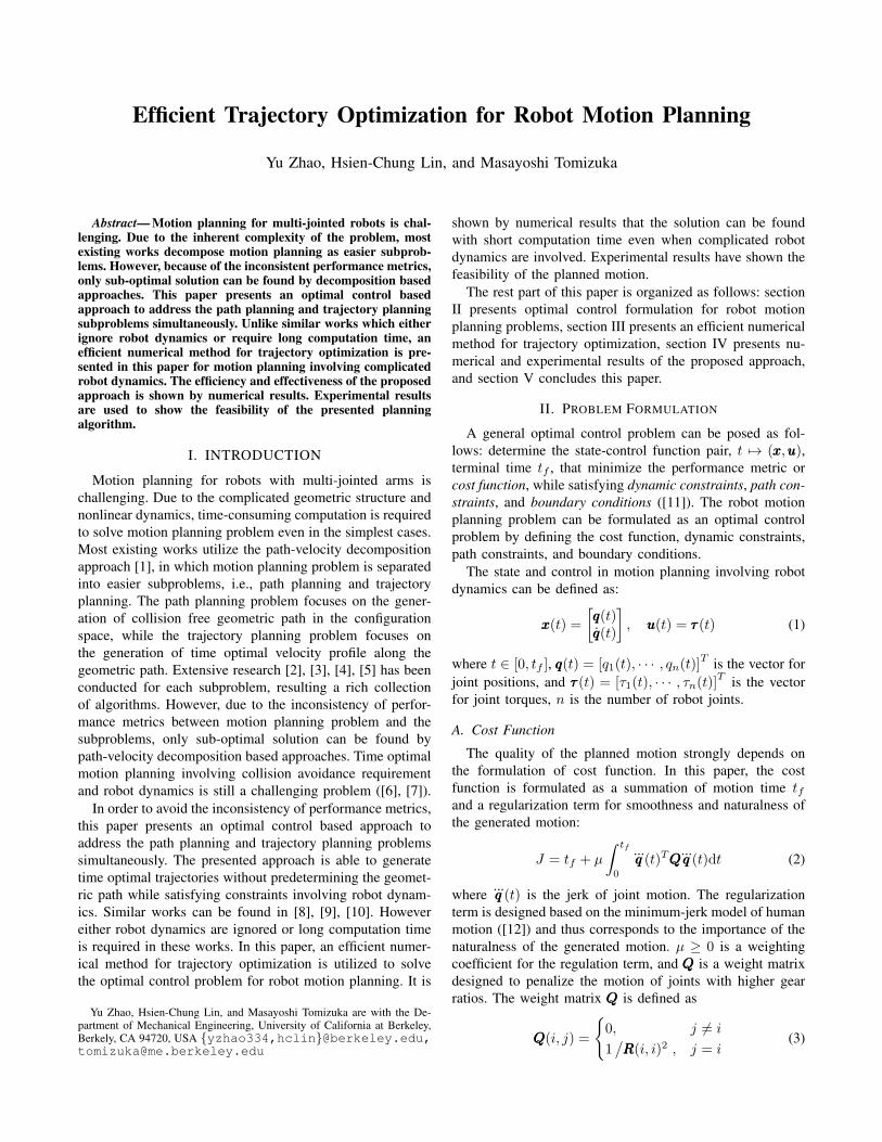
In numerical methods for trajectory optimization, two parts

are playing the key role: discretization and optimization.

An efficient implementation can be designed by choosing

Constraints

Objective

Solution

SolverCost Function

Dynamic

Constraints

Path Constraints

Boundary

Conditions

Discretization

(Pseudospectral)

Nonlinear

Optimization

Solver

Interpolation

Automatic

Differentiation

Solution

Fig. 2: Efficient numerical method for trajectory optimization

these two components intelligently. In this paper, the pseu-

dospectral method is chosen to transcribe the continuous time

optimal control problem, and the interior point method with

the support of automatic differentiation is chosen to solve

the discretized optimization problem, as illustrated in Fig. 2.

A. Pseudospectral Method

The decision variables in the continuous time optimal

control problem for robot motion planning include tf , xxx(t),and uuu(t). In the transcription procedure, xxx(t) and uuu(t) are

discretized by their values at certain time as {xxx(Ti), i =0, · · ·N} and {uuu(Ti), i = 0, · · ·N}, where {Ti, i = 0, · · ·N}are called knots, and N is the number of knots. It is

reported in previous research [14], [17], [18] that the solution

accuracy increases exponentially fast with the increase of

interpolation knots for pseudospectral methods. Thus high

computational efficiency can be achieved using pseudospec-

tral method since less discretization knots can be chosen

under the same solution accuracy requirement. In addition,

the approximate solution is guaranteed to be smooth since

high order global polynomial interpolation is utilized in

pseudospectral methods.

In this paper, the Chebyshev-Lobatto points (or Chebyshev

points) are chosen to be the knots. Such choice can avoid

the oscillation phenomenon in high order global polynomial

interpolation. For t ∈ [0, tf ], the knots are:

Ti =tf

2

[

cos

(

iπ

N

)

+ 1

]

, i = 0, · · · , N (11)

Pseudospectral methods have provided a set of tools for

polynomial interpolation, approximating integration terms

using quadrature, and approximating derivatives using dif-

ferential matrix.

1) Interpolation The polynomial interpolation in pseu-

dospectral methods can be performed by barycentric

interpolation, which can be formulated as a linear

combination of Lagrangian polynomials. For state tra-

jectory and control trajectory, the form is

xxx(t) ≈

N∑

j=0

xxx(Tj)ℓj(t)

uuu(t) ≈N∑

j=0

uuu(Tj)ℓj(t)

(12)

where ℓj(t) is the jth Lagrange polynomial. In

barycentric interpolation, a special form of Lagrange

polynomial is implemented to efficiently perform in-

terpolation ([18], [19]).

2) Quadrature Quadrature is the standard term for the

numerical calculation of integrals. The integration

of function L[xxx] can be approximately evaluated by

quadrature rules in pseudospectral methods as:

∫ tf

0

L[xxx]dt ≈

∫ tf

0

N∑

j=0

ℓj(t)L[xxx(Tj)]

dt

=

N∑

j=0

wjL[xxx(Tj)]

(13)

where {wj , j = 0, · · · , N} is a set of quadrature

weights. The quadrature weights can be explicitly

defined to be

wj =

∫ tf

0

ℓj(t)dt, j = 0, · · · , N (14)

When Chebyshev points are chosen, the corresponding

quadrature rule (Clenshaw–Curtis quadrature) can be

found in [20]:

3) Differentiation matrix Let the stacked state and robot

dynamics at knots be

XXX =

xxx(T0)T

...

xxx(TN )T

,FFF =

FFF (xxx(T0),uuu(T0))T

...

FFF (xxx(TN ),uuu(TN ))T

(15)

The dynamic constraints can be posed as [14]:

DDDXXX =tf

2FFF (16)

where DDD is the differential matrix that is used to

compute the scaled time derivative of the polynomial

approximation of xxx ([19]). Let the stacked joint torques

be UUU = [uuu(T0), · · · ,uuu(TN )]T , the stacked torque rates

UUUd = [uuu(T0), · · · , uuu(TN )]T can be approximately

calculated as:

UUUd ≈2

tfDDDUUU (17)

B. Automatic Differentiation

Lots of optimization solvers are based on gradient descent

algorithm. Derivative of objective function and constraints

are frequently evaluated by numerical differentiation ap-

proaches, which perturbs input to the function in each

dimension to obtain an approximation of the derivative

using finite differences. However, numerical differentiation

approaches are computationally expensive for functions with

high dimensional input, and inevitably introduces round-off

errors. Symbolic differentiation is one way to avoid round-

off errors, however it frequently leads to inefficient code.

Both numerical differentiation and symbolic differentiation

are problematic in the calculation of higher order derivatives

like Hessian.

To address the problems in numerical differentiation and

symbolic differentiation, automatic differentiation is intro-

duced. Automatic differentiation is a set of techniques to

evaluate derivative of a function ([21]). The computational

cost of automatic differentiation is lower than numerical

differentiation or symbolic differentiation. A rich collection

of automatic differentiation implementations can be found

in [22], [23], [24]. In this paper, CasADi [25] is chosen

for its good usability in MATLAB environment. Since com-

putational cost of automatic differentiation is proportional

to that for function evaluation, articulated body algorithm

[26] is utilized in this work for efficient evaluation of robot

dynamics.

IV. NUMERICAL AND EXPERIMENTAL RESULTS

Motion planning of a 6-axis industrial robot with dynamic

constraints is considered as an example. The industrial robot

0

-1

0.5

Z [m

]

-0.5

1

1.5

0

X [m]

0.50.5

Y [m]1

01.5

-0.52

Workspace boundary

Robot

Obstacle

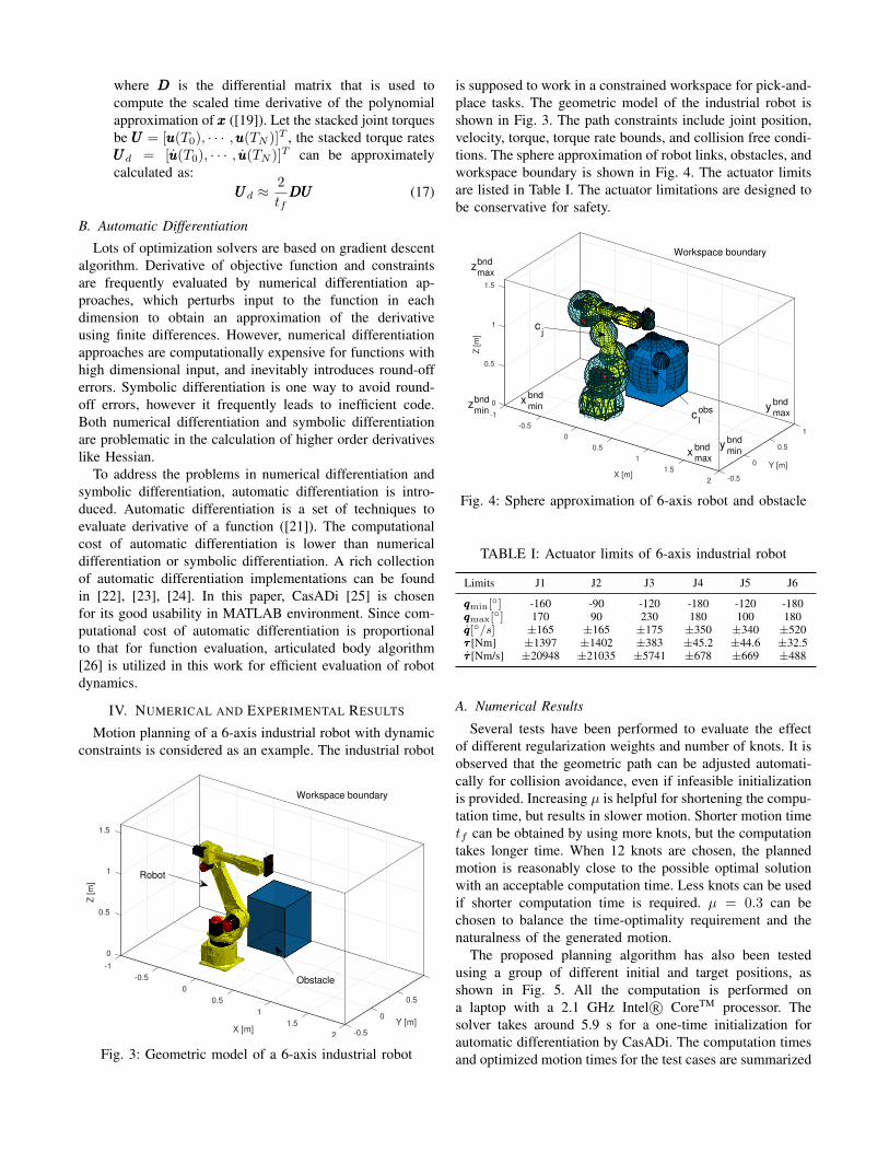
Fig. 3: Geometric model of a 6-axis industrial robot

is supposed to work in a constrained workspace for pick-and-

place tasks. The geometric model of the industrial robot is

shown in Fig. 3. The path constraints include joint position,

velocity, torque, torque rate bounds, and collision free condi-

tions. The sphere approximation of robot links, obstacles, and

workspace boundary is shown in Fig. 4. The actuator limits

are listed in Table I. The actuator limitations are designed to

be conservative for safety.

0

-1

0.5

Z [m

]

-0.5

1

1

1.5

0

X [m]

0.50.5

Y [m]1

01.5

-0.52

Workspace boundary

ybnd

min

ybnd

max

xbnd

max

xbnd

minzbnd

min

zbnd

max

cj

cobs

l

Fig. 4: Sphere approximation of 6-axis robot and obstacle

TABLE I: Actuator limits of 6-axis industrial robot

Limits J1 J2 J3 J4 J5 J6

qqqmin[◦] -160 -90 -120 -180 -120 -180

qqqmax[◦] 170 90 230 180 100 180qqq[◦/s] ±165 ±165 ±175 ±350 ±340 ±520τττ [Nm] ±1397 ±1402 ±383 ±45.2 ±44.6 ±32.5τττ [Nm/s] ±20948 ±21035 ±5741 ±678 ±669 ±488

A. Numerical Results

Several tests have been performed to evaluate the effect

of different regularization weights and number of knots. It is

observed that the geometric path can be adjusted automati-

cally for collision avoidance, even if infeasible initialization

is provided. Increasing µ is helpful for shortening the compu-

tation time, but results in slower motion. Shorter motion time

tf can be obtained by using more knots, but the computation

takes longer time. When 12 knots are chosen, the planned

motion is reasonably close to the possible optimal solution

with an acceptable computation time. Less knots can be used

if shorter computation time is required. µ = 0.3 can be

chosen to balance the time-optimality requirement and the

naturalness of the generated motion.

The proposed planning algorithm has also been tested

using a group of different initial and target positions, as

shown in Fig. 5. All the computation is performed on

a laptop with a 2.1 GHz Intel R© CoreTM processor. The

solver takes around 5.9 s for a one-time initialization for

automatic differentiation by CasADi. The computation times

and optimized motion times for the test cases are summarized

00

0.2

-0.5

0.4

0.6

0.8

Z [m

]

X [m]

1

0.5

1.2

0

10.5Y [m]1.51

(a) Test case 1

00

0.2

-0.5

0.4

0.6

0.8

Z [m

]

X [m]

1

0.5

1.2

0

Y [m]10.5

1.51

(b) Test case 2

00

0.2

-0.5

0.4

0.6

0.8

X [m]

Z [m

]

1

0.5

1.2

0

1.4

Y [m]10.5

1.51

(c) Test case 3

00

0.2

-0.5

0.4

0.6

0.8

X [m]

Z [m

]

1

0.5

1.2

0

1.4

Y [m] 10.5

1.51

(d) Test case 4

Fig. 5: Optimal multiple joint robot trajectory with different

initial and target positions, 12 knots, µ = 0.3

TABLE II: Motion time and computation time for test cases

time [s] knots case 1 case 2 case 3 case 4

motion time tf12 1.65 1.23 1.05 1.088 1.98 1.23 1.09 1.11

computation time12 2.55 2.37 2.39 2.578 1.28 1.75 0.84 1.32

in Table II. In all the test cases, good approximations of the

time optimal trajectories are returned in about 2-3 seconds

using 12 knots, and about 1-2 seconds using 8 knots. Existing

works [9], [10] require from 20 seconds to several minutes

for computation, in which only robot dynamics are involved

but not collision avoidance. The proposed approach is highly

efficient comparing to these results.

B. Experimental Results

The planned optimal trajectory of test case 2 in Fig. 5

has been used as motion reference in experiment at the

Mechanical Systems Control laboratory at the University of

California, Berkeley. The actual robot motions are captured

from video record as shown in Fig. 6. As shown in the figure,

the planned motion is collision free.

The scaled joint velocities and joint torques are shown in

Fig. 7. As shown in the figure, the planned motion is feasible

under conservative actuator limitations. The motion time tfis adjusted automatically from an initial value 10 s to about

1.2s. It is also observed that the planned motion is close to

time-optimal with at least one of the constraints is active.

(a) t = 0 s (b) t = 0.33 s

(c) t = 0.56 s (d) t = 0.8 s

(e) t = 0.96 s (f) t = 1.2 s

Fig. 6: Actual robot motion in experiment

V. CONCLUSION

Motion planning involving complicated robot dynamics

and geometric constraints is challenging. Since most ap-

proaches decompose motion planning to two subtopics and

0 0.2 0.4 0.6 0.8 1 1.2-0.8

-0.6

-0.4

-0.2

0

0.2

0.4

0.6

joint 1

joint 2

joint 3

joint 4

joint 5

joint 6

(a) Joint velocity

0 0.2 0.4 0.6 0.8 1 1.2-1

-0.5

0

0.5

1joint 1

joint 2

joint 3

joint 4

joint 5

joint 6

(b) Joint torque

Fig. 7: Measured joint velocity and torque of optimal robot

trajectory in experiment

deal with them separately, only suboptimal solution can be

found. This paper presents an optimal control based approach

to address the path planning and trajectory planning problems

simultaneously. An efficient numerical method for trajectory

optimization is proposed as one practical solution for the

nonlinear optimal control problem. Numerical results have

shown that the motion planning problem can be solved with a

short computation time and reasonable accuracy. Experimen-

tal results have verified the effectiveness and feasibility of the

planning algorithm. It is worth investigating improvements

to this approach and exploring possibilities to implement it

in different robotic applications.

REFERENCES

[1] Q.-C. Pham, S. Caron, P. Lertkultanon, and Y. Nakamura, “Admissiblevelocity propagation: Beyond quasi-static path planning for high-dimensional robots,” The International Journal of Robotics Research,vol. 36, no. 1, pp. 44–67, 2017.

[2] S. M. LaValle, Planning algorithms. Cambridge university press,2006.

[3] I. A. Sucan, M. Moll, and L. E. Kavraki, “The open motion planninglibrary,” IEEE Robotics & Automation Magazine, vol. 19, no. 4, pp.72–82, 2012.

[4] D. Verscheure, B. Demeulenaere, J. Swevers, J. De Schutter, andM. Diehl, “Time-optimal path tracking for robots: A convex opti-mization approach,” IEEE Transactions on Automatic Control, vol. 54,no. 10, pp. 2318–2327, 2009.

[5] P. Reynoso-Mora, W. Chen, and M. Tomizuka, “A convex relaxationfor the time-optimal trajectory planning of robotic manipulators along

predetermined geometric paths,” Optimal Control Applications and

Methods, vol. 37, no. 6, pp. 1263–1281, 2016.[6] S. M. La Valle, “Motion planning,” IEEE Robotics & Automation

Magazine, vol. 18, no. 2, pp. 108–118, 2011.[7] Q.-C. Pham, “A general, fast, and robust implementation of the

time-optimal path parameterization algorithm,” IEEE Transactions on

Robotics, vol. 30, no. 6, pp. 1533–1540, 2014.[8] J. Schulman, J. Ho, A. X. Lee, I. Awwal, H. Bradlow, and P. Abbeel,

“Finding locally optimal, collision-free trajectories with sequentialconvex optimization.” in Robotics: science and systems, vol. 9, no. 1.Citeseer, 2013, pp. 1–10.

[9] T. Chettibi, H. Lehtihet, M. Haddad, and S. Hanchi, “Minimumcost trajectory planning for industrial robots,” European Journal of

Mechanics-A/Solids, vol. 23, no. 4, pp. 703–715, 2004.[10] M. Diehl, H. G. Bock, H. Diedam, and P.-B. Wieber, “Fast direct

multiple shooting algorithms for optimal robot control,” in Fast

motions in biomechanics and robotics. Springer, 2006, pp. 65–93.[11] I. M. Ross and M. Karpenko, “A review of pseudospectral optimal

control: From theory to flight,” Annual Reviews in Control, vol. 36,no. 2, pp. 182–197, 2012.

[12] T. Flash and N. Hogan, “The coordination of arm movements: an ex-perimentally confirmed mathematical model,” Journal of neuroscience,vol. 5, no. 7, pp. 1688–1703, 1985.

[13] G. Bradshaw and C. O’Sullivan, “Adaptive medial-axis approximationfor sphere-tree construction,” ACM Transactions on Graphics (TOG),vol. 23, no. 1, pp. 1–26, 2004.

[14] A. V. Rao, “A survey of numerical methods for optimal control,”Advances in the Astronautical Sciences, vol. 135, no. 1, pp. 497–528,2009.

[15] J. T. Betts, Practical methods for optimal control and estimation using

nonlinear programming. Siam, 2010, vol. 19.[16] M. P. Kelly, “Transcription methods for trajectory optimization,”

Tutorial, Cornell University, Feb, 2015.[17] M. Kelly, “An introduction to trajectory optimization: How to do your

own direct collocation,” SIAM Review, vol. 59, no. 4, pp. 849–904,2017.

[18] L. N. Trefethen, Approximation theory and approximation practice.Siam, 2013, vol. 128.

[19] J.-P. Berrut and L. N. Trefethen, “Barycentric lagrange interpolation,”SIAM review, vol. 46, no. 3, pp. 501–517, 2004.

[20] J. Waldvogel, “Fast construction of the fejer and clenshaw–curtisquadrature rules,” BIT Numerical Mathematics, vol. 46, no. 1, pp.195–202, 2006.

[21] A. Griewank and A. Walther, Evaluating derivatives: principles and

techniques of algorithmic differentiation. Siam, 2008, vol. 105.[22] A. Walther and A. Griewank, “Getting started with adol-c.” in Com-

binatorial scientific computing, 2009, pp. 181–202.[23] B. M. Bell, “Cppad: a package for c++ algorithmic differentiation,”

Computational Infrastructure for Operations Research, vol. 57, 2012.[24] C. Bendtsen and O. Stauning, “Fadbad, a flexible c++ package

for automatic differentiation,” Technical Report IMM–REP–1996–17, Department of Mathematical Modelling, Technical University ofDenmark, Lyngby, Denmark, Tech. Rep., 1996.

[25] J. A. E. Andersson, J. Gillis, G. Horn, J. B. Rawlings, and M. Diehl,“CasADi – A software framework for nonlinear optimization andoptimal control,” Mathematical Programming Computation, In Press,2018.

[26] R. Featherstone, Rigid body dynamics algorithms. Springer, 2014.