TRAJECTORY CONTROL OF A TWO-WHEELED ROBOT

University of Rhode Island University of Rhode Island

DigitalCommons@URI DigitalCommons@URI

Open Access Master's Theses

2012

TRAJECTORY CONTROL OF A TWO-WHEELED ROBOT TRAJECTORY CONTROL OF A TWO-WHEELED ROBOT

Michael D. Peltier University of Rhode Island, [email protected]

Follow this and additional works at: https://digitalcommons.uri.edu/theses

Recommended Citation Recommended Citation Peltier, Michael D., "TRAJECTORY CONTROL OF A TWO-WHEELED ROBOT" (2012). Open Access Master's Theses. Paper 94. https://digitalcommons.uri.edu/theses/94

This Thesis is brought to you for free and open access by DigitalCommons@URI. It has been accepted for inclusion in Open Access Master's Theses by an authorized administrator of DigitalCommons@URI. For more information, please contact [email protected].

https://digitalcommons.uri.edu/

https://digitalcommons.uri.edu/theses

https://digitalcommons.uri.edu/theses?utm_source=digitalcommons.uri.edu%2Ftheses%2F94&utm_medium=PDF&utm_campaign=PDFCoverPages

https://digitalcommons.uri.edu/theses/94?utm_source=digitalcommons.uri.edu%2Ftheses%2F94&utm_medium=PDF&utm_campaign=PDFCoverPages

mailto:[email protected]

TRAJECTORY CONTROL OF A TWO-WHEELED ROBOT

BY

MICHAEL D. PELTIER

A THESIS SUBMITTED IN PARTIAL FULFILLMENT OF THE

REQUIREMENTS FOR THE DEGREE OF

MASTER OF SCIENCE

IN

ELECTRICAL ENGINEERING

UNIVERSITY OF RHODE ISLAND

2012

MASTER OF SCIENCE THESIS

OF

MICHAEL D. PELTIER

APPROVED:

Thesis Committee:

Major Professor Richard J. Vaccaro

Peter F. Swaszek

William J. Palm

Nasser H. Zawia

DEAN OF THE GRADUATE SCHOOL

UNIVERSITY OF RHODE ISLAND

2012

ABSTRACT

Robots have been used in many applications in the past three decades. One

type of robot is a two-wheeled robot that requires control for both balancing and

maneuvering. This thesis shows the design of a controller that can both balance

and provide trajectory control for a two-wheeled robot. The controller is a dig-

ital tracking system that utilizes pole placement for system stability. The thesis

provides a detailed description for modeling the plant, design of the controller,

simulating the final system and implementation into hardware. Three pole place-

ment methods are analyzed as well as tracking designs that use steady-state or

ramp tracking. Each of these controllers have simulation results and the controller

that has the best simulation performance is implemented into the hardware. The

final controller is implemented into Lego R© Mindstorm R© hardware using Matlab R©

and Simulink R©. The results of the simulations are compared to the results found

in hardware.

ACKNOWLEDGMENTS

I would like to acknowledge Dr. Richard J. Vaccaro for his guidance and advice

in the area of control theory. The knowledge he has provided was instrumental

in the completion of this thesis. I would also like to thank my wife Dr. Dena L.

Peltier for her support and patience.

iii

TABLE OF CONTENTS

ABSTRACT . . . . . . . . . . . . . . . . . . . . . . . . . . . . . . . . . . ii

ACKNOWLEDGMENTS . . . . . . . . . . . . . . . . . . . . . . . . . . iii

TABLE OF CONTENTS . . . . . . . . . . . . . . . . . . . . . . . . . . iv

LIST OF TABLES . . . . . . . . . . . . . . . . . . . . . . . . . . . . . . . vii

LIST OF FIGURES . . . . . . . . . . . . . . . . . . . . . . . . . . . . . . viii

CHAPTER

1 Introduction . . . . . . . . . . . . . . . . . . . . . . . . . . . . . . . 1

1.1 Problem Identification . . . . . . . . . . . . . . . . . . . . . . . 1

1.2 Contributions of this Thesis . . . . . . . . . . . . . . . . . . . . 2

1.3 Overview of this Thesis . . . . . . . . . . . . . . . . . . . . . . . 2

List of References . . . . . . . . . . . . . . . . . . . . . . . . . . . . . 3

2 Two-Wheeled Robot Model . . . . . . . . . . . . . . . . . . . . . 4

2.1 State-Space Equations . . . . . . . . . . . . . . . . . . . . . . . 7

2.2 Experimental Parameters . . . . . . . . . . . . . . . . . . . . . . 9


3 Digital Tracking System Theory . . . . . . . . . . . . . . . . . . 12

3.1 Controllability . . . . . . . . . . . . . . . . . . . . . . . . . . . . 13

3.2 Tracking System . . . . . . . . . . . . . . . . . . . . . . . . . . . 14

3.3 Additional Dynamics . . . . . . . . . . . . . . . . . . . . . . . . 15

3.4 Feedback Matrix . . . . . . . . . . . . . . . . . . . . . . . . . . 15

iv

Page

v

3.5 Stability Margins . . . . . . . . . . . . . . . . . . . . . . . . . . 19


4 Hardware . . . . . . . . . . . . . . . . . . . . . . . . . . . . . . . . 22

4.1 Architecture . . . . . . . . . . . . . . . . . . . . . . . . . . . . . 22

4.2 Design Tools . . . . . . . . . . . . . . . . . . . . . . . . . . . . . 24

4.3 Bluetooth Interface . . . . . . . . . . . . . . . . . . . . . . . . . 24

4.4 GUI . . . . . . . . . . . . . . . . . . . . . . . . . . . . . . . . . 25

4.5 Controller Design Considerations . . . . . . . . . . . . . . . . . 27


5 Controller Design . . . . . . . . . . . . . . . . . . . . . . . . . . . 29

5.1 Additional Dynamics . . . . . . . . . . . . . . . . . . . . . . . . 30

5.2 Feedback Matrix . . . . . . . . . . . . . . . . . . . . . . . . . . 31


5.4 Plant Inputs and Outputs . . . . . . . . . . . . . . . . . . . . . 33

6 Modeling and Simulations . . . . . . . . . . . . . . . . . . . . . . 35

6.1 Performance Testing . . . . . . . . . . . . . . . . . . . . . . . . 36

6.2 Figure Eight Tracking . . . . . . . . . . . . . . . . . . . . . . . . 48

7 Hardware Testing . . . . . . . . . . . . . . . . . . . . . . . . . . . 58

7.1 Balancing . . . . . . . . . . . . . . . . . . . . . . . . . . . . . . 63

7.2 Theta Ramping . . . . . . . . . . . . . . . . . . . . . . . . . . . 68

7.3 Phi Ramping . . . . . . . . . . . . . . . . . . . . . . . . . . . . 72

7.4 Figure Eight . . . . . . . . . . . . . . . . . . . . . . . . . . . . . 77

Page

vi

8 Conclusions . . . . . . . . . . . . . . . . . . . . . . . . . . . . . . . 83


APPENDIX

Matlab Code . . . . . . . . . . . . . . . . . . . . . . . . . . . . . . . . 86

BIBLIOGRAPHY . . . . . . . . . . . . . . . . . . . . . . . . . . . . . . . 91

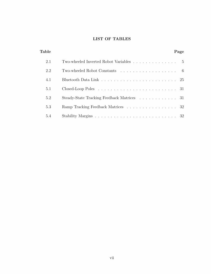
LIST OF TABLES

Table Page

2.1 Two-wheeled Inverted Robot Variables . . . . . . . . . . . . . . 5

2.2 Two-wheeled Robot Constants . . . . . . . . . . . . . . . . . . 6

4.1 Bluetooth Data Link . . . . . . . . . . . . . . . . . . . . . . . . 25

5.1 Closed-Loop Poles . . . . . . . . . . . . . . . . . . . . . . . . . 31

5.2 Steady-State Tracking Feedback Matrices . . . . . . . . . . . . 31

5.3 Ramp Tracking Feedback Matrices . . . . . . . . . . . . . . . . 32


vii

LIST OF FIGURES

Figure Page

2.1 Two-wheeled Robot [1] . . . . . . . . . . . . . . . . . . . . . . . 4

2.2 Side and Plane View of Two-wheeled Robot [1] . . . . . . . . . 5

3.1 Digital Tracking System . . . . . . . . . . . . . . . . . . . . . . 14

4.1 LEGO Two-wheeled Robot . . . . . . . . . . . . . . . . . . . . 22

4.2 Hardware Architecture . . . . . . . . . . . . . . . . . . . . . . . 23

4.3 Gyro Sensor . . . . . . . . . . . . . . . . . . . . . . . . . . . . . 24

4.4 Control GUI . . . . . . . . . . . . . . . . . . . . . . . . . . . . . 26

6.1 Simulink Model . . . . . . . . . . . . . . . . . . . . . . . . . . . 35

6.2 Controller . . . . . . . . . . . . . . . . . . . . . . . . . . . . . . 36

6.3 Steady-State φ Tracking Voltage Commands . . . . . . . . . . . 38

6.4 Steady-State φ Tracking Measured θ State . . . . . . . . . . . . 38

6.5 Steady-State φ Tracking . . . . . . . . . . . . . . . . . . . . . . 39

6.6 Steady-State φ Tracking Measured Ψ State . . . . . . . . . . . . 39

6.7 Steady-State θ Tracking Voltage Commands . . . . . . . . . . . 40

6.8 Steady-State θ Tracking . . . . . . . . . . . . . . . . . . . . . . 41

6.9 Steady-State θ Tracking Measured φ State . . . . . . . . . . . . 41

6.10 Steady-State θ Tracking Measured Ψ State . . . . . . . . . . . . 42

6.11 Ramping φ Tracking Voltage Commands . . . . . . . . . . . . . 43

6.12 Ramping φ Tracking Measured θ State . . . . . . . . . . . . . . 44

6.13 Ramping φ Tracking . . . . . . . . . . . . . . . . . . . . . . . . 44

6.14 Ramping φ Tracking Measured Ψ State . . . . . . . . . . . . . . 45

viii

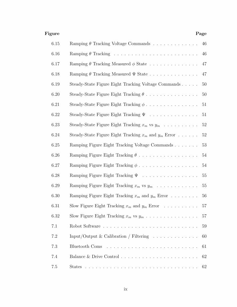
Figure Page

ix

6.15 Ramping θ Tracking Voltage Commands . . . . . . . . . . . . . 46

6.16 Ramping θ Tracking . . . . . . . . . . . . . . . . . . . . . . . . 46

6.17 Ramping θ Tracking Measured φ State . . . . . . . . . . . . . . 47

6.18 Ramping θ Tracking Measured Ψ State . . . . . . . . . . . . . . 47

6.19 Steady-State Figure Eight Tracking Voltage Commands . . . . . 50

6.20 Steady-State Figure Eight Tracking θ . . . . . . . . . . . . . . . 50

6.21 Steady-State Figure Eight Tracking φ . . . . . . . . . . . . . . . 51

6.22 Steady-State Figure Eight Tracking Ψ . . . . . . . . . . . . . . 51

6.23 Steady-State Figure Eight Tracking xm vs ym . . . . . . . . . . 52

6.24 Steady-State Figure Eight Tracking xm and ym Error . . . . . . 52

6.25 Ramping Figure Eight Tracking Voltage Commands . . . . . . . 53

6.26 Ramping Figure Eight Tracking θ . . . . . . . . . . . . . . . . . 54

6.27 Ramping Figure Eight Tracking φ . . . . . . . . . . . . . . . . . 54

6.28 Ramping Figure Eight Tracking Ψ . . . . . . . . . . . . . . . . 55

6.29 Ramping Figure Eight Tracking xm vs ym . . . . . . . . . . . . 55

6.30 Ramping Figure Eight Tracking xm and ym Error . . . . . . . . 56

6.31 Slow Figure Eight Tracking xm and ym Error . . . . . . . . . . 57

6.32 Slow Figure Eight Tracking xm vs ym . . . . . . . . . . . . . . . 57

7.1 Robot Software . . . . . . . . . . . . . . . . . . . . . . . . . . . 59

7.2 Input/Output & Calibration / Filtering . . . . . . . . . . . . . 60

7.3 Bluetooth Coms . . . . . . . . . . . . . . . . . . . . . . . . . . 61

7.4 Balance & Drive Control . . . . . . . . . . . . . . . . . . . . . . 62

7.5 States . . . . . . . . . . . . . . . . . . . . . . . . . . . . . . . . 62

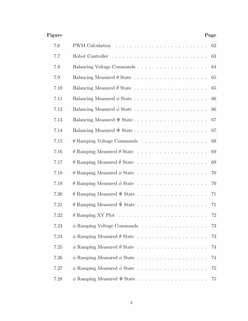
Figure Page

x

7.6 PWM Calculation . . . . . . . . . . . . . . . . . . . . . . . . . 62

7.7 Robot Controller . . . . . . . . . . . . . . . . . . . . . . . . . . 63

7.8 Balancing Voltage Commands . . . . . . . . . . . . . . . . . . . 64

7.9 Balancing Measured θ State . . . . . . . . . . . . . . . . . . . . 65

7.10 Balancing Measured θ State . . . . . . . . . . . . . . . . . . . . 65

7.11 Balancing Measured φ State . . . . . . . . . . . . . . . . . . . . 66

7.12 Balancing Measured φ State . . . . . . . . . . . . . . . . . . . . 66

7.13 Balancing Measured Ψ State . . . . . . . . . . . . . . . . . . . . 67

7.14 Balancing Measured Ψ State . . . . . . . . . . . . . . . . . . . . 67

7.15 θ Ramping Voltage Commands . . . . . . . . . . . . . . . . . . 68

7.16 θ Ramping Measured θ State . . . . . . . . . . . . . . . . . . . 69

7.17 θ Ramping Measured θ State . . . . . . . . . . . . . . . . . . . 69

7.18 θ Ramping Measured φ State . . . . . . . . . . . . . . . . . . . 70

7.19 θ Ramping Measured φ State . . . . . . . . . . . . . . . . . . . 70

7.20 θ Ramping Measured Ψ State . . . . . . . . . . . . . . . . . . . 71

7.21 θ Ramping Measured Ψ State . . . . . . . . . . . . . . . . . . . 71

7.22 θ Ramping XY Plot . . . . . . . . . . . . . . . . . . . . . . . . 72

7.23 φ Ramping Voltage Commands . . . . . . . . . . . . . . . . . . 73

7.24 φ Ramping Measured θ State . . . . . . . . . . . . . . . . . . . 73

7.25 φ Ramping Measured θ State . . . . . . . . . . . . . . . . . . . 74

7.26 φ Ramping Measured φ State . . . . . . . . . . . . . . . . . . . 74

7.27 φ Ramping Measured φ State . . . . . . . . . . . . . . . . . . . 75

7.28 φ Ramping Measured Ψ State . . . . . . . . . . . . . . . . . . . 75

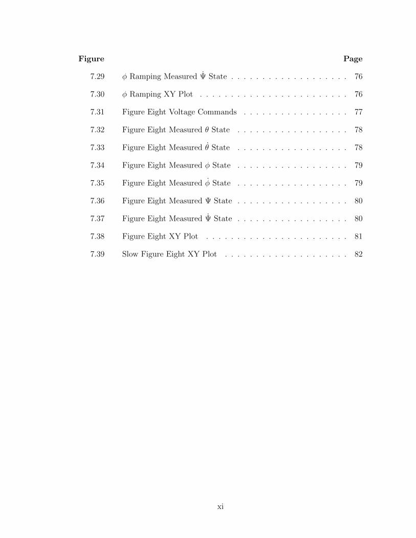
Figure Page

xi

7.29 φ Ramping Measured Ψ State . . . . . . . . . . . . . . . . . . . 76

7.30 φ Ramping XY Plot . . . . . . . . . . . . . . . . . . . . . . . . 76

7.31 Figure Eight Voltage Commands . . . . . . . . . . . . . . . . . 77

7.32 Figure Eight Measured θ State . . . . . . . . . . . . . . . . . . 78

7.33 Figure Eight Measured θ State . . . . . . . . . . . . . . . . . . 78

7.34 Figure Eight Measured φ State . . . . . . . . . . . . . . . . . . 79

7.35 Figure Eight Measured φ State . . . . . . . . . . . . . . . . . . 79

7.36 Figure Eight Measured Ψ State . . . . . . . . . . . . . . . . . . 80

7.37 Figure Eight Measured Ψ State . . . . . . . . . . . . . . . . . . 80

7.38 Figure Eight XY Plot . . . . . . . . . . . . . . . . . . . . . . . 81

7.39 Slow Figure Eight XY Plot . . . . . . . . . . . . . . . . . . . . 82

CHAPTER 1

Introduction

The ability to control robots has been in the forefront of control theory in

the past three decades. Robots have been used in many applications. They can

be used to make everyday living for the handicapped easier while allowing tasks

to be performed more efficiently in industry. These robots are becoming more

sophisticated to where they can autonomously perform tasks.

The control of each type of robot becomes its own engineering problem.

Robots can move around using wheels, tracks or belts. They may even stay in

place and perform tasks along an assembly line. The actuators can be electrome-

chanical or use hydraulics. All these differences result in different kinematics and

dynamics of the robot.

There are many examples of controlling an inverted pendulum. Seul Jung and

Sung Su Kim [1] use a Neural Network to provide tracking control for a single-

input-multiple-output (SIMO) two-wheeled robot. The cart is controlled forward

and back, tracking a sinusoidal motion. Vaccaro [2] uses digital state feedback

tracking to control a SIMO inverted pendulum that uses a cart coupled to a drive

screw. In work introduced by S.W. Nawawi et al, [3] a sliding mode controller

was used to balance a two-wheeled robot; however, it does not indicate that the

controller can be used to control the robot’s trajectory.

1.1 Problem Identification

The two-wheeled robot is an inverted pendulum that can also move about in

a two dimensional plane. The robot contains sensors that provide feedback for

balancing and trajectory tracking. Pole placement will be used in the design of

the controller. Therefore, the two-wheeled robot will need to be modeled. Since

1

pole placement is used to design the controller the method of placement needs to

be scrutinized for both stability and performance. Consideration will also need to

be taken when implementing the new controller in real hardware.

1.2 Contributions of this Thesis

The two-wheeled robot has some challenges that are not seen in the inverted

pendulum problem. In the inverted pendulum problem found in the book by

Vaccaro [2], the pendulum is mounted to a cart. The cart is directly coupled to

the drive motor, while the pendulum moves freely on a mounted encoder. The

two-wheeled robot has the inverted pendulum directly coupled to the drive motor.

Also, the inverted pendulum rotates on a single shaft. The two-wheeled robot does

not rotate on one shaft, but uses two shafts, one for each wheel. This problem

was examined by Yamamoto [4] by controlling the average of the two wheels.

Yamamoto was successful in creating a closed-loop control for balancing; however,

the controller did not provide closed-loop control for trajectory tracking. Rather

than control the average of the wheels (a single control input), the controller in this

thesis will send independent coordinated signals to each motor (two control inputs).

The design of this system will require the tools of multivariable control theory.

Tests with the hardware robot will demonstrate the applicability of multivariable

control theory to a real-world system. Modifications may have to be made for the

theoretical results to be implemented in hardware.

1.3 Overview of this Thesis

The research for this master’s thesis will require a scientific approach. The

dynamics of the system need to be carefully scrutinized and also the micro con-

troller architecture, which can introduce delays [5]. A plant model exists [4] and

some system parameters will be found directly from measurements of the hardware

2

system. The final plant will be used to design a controller based on Digital Track-

ing System Theory. The design will include a comparison of multiple methods

used to calculate a feedback matrix for the desired closed-loop pole locations, and

a stability analysis to determine robustness. Simulations will be used to observe

the response of the system. The controller that provides the best stability margins

and performance will be loaded into hardware for testing. Finally, collected data

from the hardware and simulations will be compared.

List of References

[1] S. Jung and S. S. Kim, “Control experiment of a wheel-driven mobile in-verted pendulum using neural network,” IEEE Transactions On Control Sys-tems Technology, vol. 16, pp. 297–303, March 2008.

[2] R. J. Vaccaro, Digital Control A State-Space Approch. New York, New York,United States of America: McGraw-Hill, Inc, 1995.

[3] S. Nawawi, M. Ahmad, J. Osman, A. Husain, and M. Abdollah, “Controllerdesign for two-wheels inverted pendulum mobile robot using PISMC,” 4th Stu-dent Conference on Research and Development, pp. 194 – 199, June 2006.

[4] Y. Yamamoto, “Nxtway-gs model-based design - control of self-balancingtwo-wheeled robot built with lego mindstorms nxt -,” May 2009, unpublished.[Online]. Available: http://www.mathworks.com/matlabcentral/fileexchange/19147-nxtway-gs-self-balancing-two-wheeled-robot-controller-design?controller=file infos&download=true

[5] T. Chikamasa, “Embedded coder robot nxt mod-eling tips,” April 2010, unpublished. [Online].Available: http://www.mathworks.com/matlabcentral/fileexchange/13399-embedded-coder-robot-nxt-demo?controller=file infos&download=true

3

http://www.mathworks.com/matlabcentral/fileexchange/19147-nxtway-gs-self-balancing-two-wheeled-robot-controller-design?controller=file_infos&download=true



http://www.mathworks.com/matlabcentral/fileexchange/13399-embedded-coder-robot-nxt-demo?controller=file_infos&download=true


CHAPTER 2

Two-Wheeled Robot Model

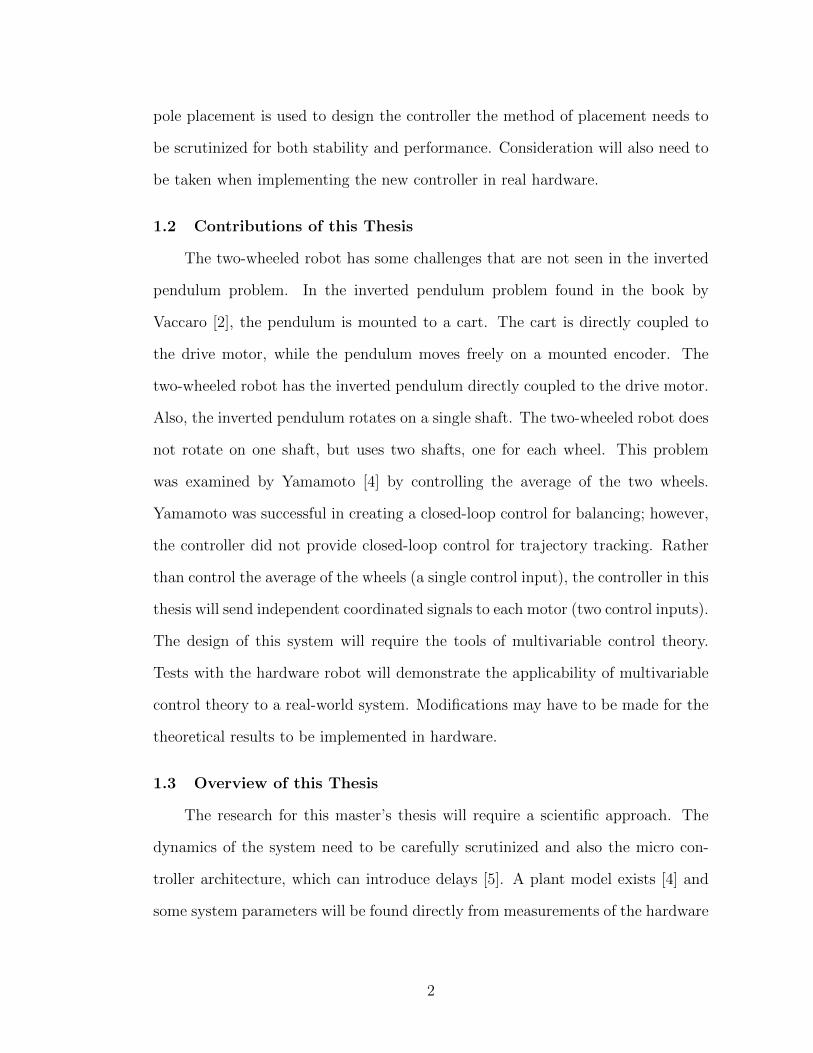
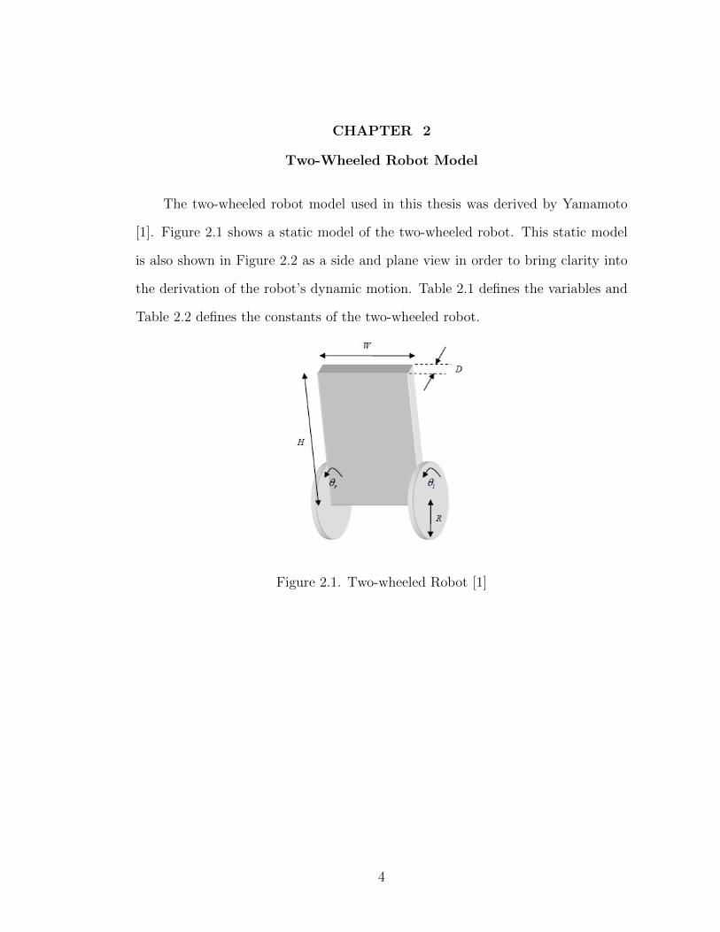
The two-wheeled robot model used in this thesis was derived by Yamamoto

[1]. Figure 2.1 shows a static model of the two-wheeled robot. This static model

is also shown in Figure 2.2 as a side and plane view in order to bring clarity into

the derivation of the robot’s dynamic motion. Table 2.1 defines the variables and

Table 2.2 defines the constants of the two-wheeled robot.

Figure 2.1. Two-wheeled Robot [1]

4

Figure 2.2. Side and Plane View of Two-wheeled Robot [1]

Variable Units Descriptionθ [rad] Average angle of left and right wheelΨ [rad] Body pitch angleφ [rad] Body yaw angleθr [rad] Rotational angle of the right wheelθl [rad] Rotational angle of the left wheelθmr

[rad] DC motor angle of the right wheelθml

[rad] DC motor angle of the left wheelxm, ym, zm [m] Coordinates of the centerlinexr, yr, zr [m] Coordinates of the right wheelxl, yl, zl [m] Coordinates of the left wheelxb, yb, zb [m] Coordinates of the center of gravity

vl [V olts] Voltage applied to the left motorvr [V olts] Voltage applied to the right motor

Table 2.1. Two-wheeled Inverted Robot Variables

5

Constant Value Units Descriptiong 9.81 [m/s2] Gravity accelerationm 0.03 [kg] Wheel weightJw 2.4e-5 [kgm2] Wheel inertia momentW 0.175 [m] Width of the robot bodyD 0.04 [m] Depth of the robot bodyH 0.144 [m] Height of the robot bodyL 0.079 [m] Distance of the center of mass from the

wheel axleR 0.04 [m] Radius of the wheel

JΨML2

3[kgm2] Body pitch inertia moment

JφM(W 2+D2)

12[kgm2] Body yaw inertia moment

Rm 6.69 [Ω] DC motor resistanceKb 0.468 [V sec/rad] DC motor back EMF constantKt 0.317 [Nm/A] DC motor torque constantfm 0.0224 N/A Friction coefficient between body and DC

motor

Table 2.2. Two-wheeled Robot Constants

The state-space equation for the two-wheeled robot is based on the coordinate

system in Figure 2.2. The equations that define the motion of the two-wheeled

robot in the coordinate system are shown in Equations (2.1) through (2.7) and

have the initial heading along the positive x-axis at t = 0. These equations show

that the final state-space equation only requires the variable θ, Ψ, and φ.

(θl, θr) =(θml

+ Ψ, θmr+ Ψ

)(2.1)

(θ, φ) =

(1

2(θl + θr) ,

R

W(θr − θl)

)(2.2)

(xm, ym, zm) =

(∫xmdt,

∫ymdt, R

)(2.3)

(xm, ym) =(Rθ cosφ,Rθ sinφ

)(2.4)

(xl, yl, zl) =

(xm −

W

2sinφ, ym +

W

2cosφ, zm

)(2.5)

(xr, yr, zr) =

(xm +

W

2sinφ, ym −

W

2cosφ, zm

)(2.6)

(xb, yb, zb) = (xm + L sin Ψ cosφ, ym + L sin Ψ sinφ, zm + L cos Ψ) (2.7)

6

2.1 State-Space Equations

The state-space equation is derived from the translational kinetic energy, rota-

tional kinetic energy, potential energy, DC motor torque and the DC motor viscous

friction. Equation (2.8) is the motion equation for the two-wheeled robot for the

variables θ and Ψ.

E

[θ

Ψ

]+ F

[θ

Ψ

]+ G

[θΨ

]= H

[vlvr

](2.8)

The matrices E,F,G and H are defined in Equation (2.9) and the constants

are defined in Equation (2.10).

E =

[C1 C2C2 C3

](2.9)

F = 2×[

C4 −C4−C4 C4

]G =

[0 00 −C5

]H =

[C6 C6−C6 −C6

]

C1 = (2m+M)R2 + Jw (2.10)

C2 = MRL

C3 = ML2 + JΨ

C4 =KtKb

Rm

+ fm

C5 = MgL

C6 =Kt

Rm

Equation (2.11) is the motion equation for the two-wheeled robot for the

variable φ. The constants are defined in Equation (2.12).

Iφ+ Jφ = K(vr − vl) (2.11)

7

I =1

2mW 2 + Jφ +

W 2

2R2Jw (2.12)

J =W 2

2R2

(KtKb

Rm

+ fm

)K =

W

2R

Kt

Rm

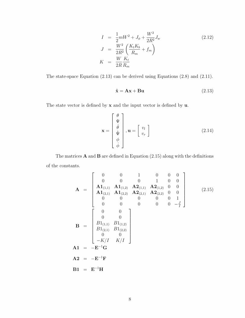
The state-space Equation (2.13) can be derived using Equations (2.8) and (2.11).

x = Ax + Bu (2.13)

The state vector is defined by x and the input vector is defined by u.

x =

θΨ

θ

Ψφ

φ

,u =

[vlvr

](2.14)

The matrices A and B are defined in Equation (2.15) along with the definitions

of the constants.

A =

0 0 1 0 0 00 0 0 1 0 0

A1(1,1) A1(1,2) A2(1,1) A2(1,2) 0 0A1(2,1) A1(2,2) A2(2,1) A2(2,2) 0 0

0 0 0 0 0 10 0 0 0 0 −J

I

(2.15)

B =

0 00 0

B1(1,1) B1(1,2)

B1(2,1) B1(2,2)

0 0−K/I K/I

A1 = −E−1G

A2 = −E−1F

B1 = E−1H

8

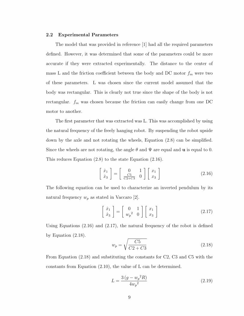
2.2 Experimental Parameters

The model that was provided in reference [1] had all the required parameters

defined. However, it was determined that some of the parameters could be more

accurate if they were extracted experimentally. The distance to the center of

mass L and the friction coefficient between the body and DC motor fm were two

of these parameters. L was chosen since the current model assumed that the

body was rectangular. This is clearly not true since the shape of the body is not

rectangular. fm was chosen because the friction can easily change from one DC

motor to another.

The first parameter that was extracted was L. This was accomplished by using

the natural frequency of the freely hanging robot. By suspending the robot upside

down by the axle and not rotating the wheels, Equation (2.8) can be simplified.

Since the wheels are not rotating, the angle θ and Ψ are equal and u is equal to 0.

This reduces Equation (2.8) to the state Equation (2.16).[x1

x3

]=

[0 1C5

C2+C30

] [x1

x3

](2.16)

The following equation can be used to characterize an inverted pendulum by its

natural frequency wp as stated in Vaccaro [2].[x1

x3

]=

[0 1wp

2 0

] [x1

x3

](2.17)

Using Equations (2.16) and (2.17), the natural frequency of the robot is defined

by Equation (2.18).

wp =

√C5

C2 + C3(2.18)

From Equation (2.18) and substituting the constants for C2, C3 and C5 with the

constants from Equation (2.10), the value of L can be determined.

L =3 (g − wp2R)

4wp2(2.19)

9

The robot was suspended by the axle and the period of oscillation was recorded

from the gyro sensor. The measured period of oscillation of the robot was 0.7647

[sec] which results in a natural frequency of 8.2165 [rad/sec]. Solving for Equation

(2.19), the distance of the center of mass to the axial, L equals 7.9 [cm].

The second parameter fm was also extracted experimentally. It was deter-

mined that the DC motor poles were fast and would be difficult to measure using

feedback over the robot’s serial bluetooth interface. Therefore, the experiment was

designed to only examine the steady-state transfer function of the DC motors. This

experiment required using a speed controller on each wheel. The robot was held

upright by a piece of string. The speed controller was then activated, commanding

both wheels to the same speed. Once the robot reached steady-state, the voltages

were recorded via the bluetooth data link.

Holding the robot upright allows Equation (2.8) to be simplified. When up-

right, Ψ and Ψ equal 0 which results in Equations (2.20) and (2.21).

C1x3 + 2(C4)x3 = C6 (vl + vr) (2.20)

C2x3 − 2(C4)x3 = −C6 (vl + vr) (2.21)

Since a speed controller is being used for the experiment, x3 in Equations (2.20)

and (2.21) drops out once the two wheels have reached a steady-state speed. Also,

setting vl and vr to u results in the Equation (2.22).

C4x3 = C6u (2.22)

The ratio for the measured output to the measured input is defined as α, where

α =x3

u=C6

C4(2.23)

Using Equation (2.23) and substituting the constants for C4 and C6 with the

constants from Equation (2.10) the value of fm can be determined.

fm =Kt

Rmα(1−Kbα) (2.24)

10

The constant α was experimentally determined to be 1.0622 [rad/(Vsec)].

Solving for Equation (2.24), the friction coefficient between the body and DC

motor, fm equals 0.0224.

List of References

[1] Y. Yamamoto, “Nxtway-gs model-based design - control of self-balancingtwo-wheeled robot built with lego mindstorms nxt -,” May 2009, unpublished.[Online]. Available: http://www.mathworks.com/matlabcentral/fileexchange/19147-nxtway-gs-self-balancing-two-wheeled-robot-controller-design?controller=file infos&download=true


11




CHAPTER 3

Digital Tracking System Theory

The two-wheeled robot must balance while maneuvering. Balancing the robot

is the well known inverted pendulum problem. However, to maneuver the robot

with closed-loop control is not an easy task. The robot as described in Equation

(2.15) has six state variables which all contribute to the stability of both maneu-

vering and balancing of the robot. The task also has an added level of difficulty

due to the fact that there are two control actuators.

The design of the controller was based on the digital tracking system in

the book by Vaccaro [1] with aid of the digital control toolbox which can be

downloaded from http://www.mathworks.com/matlabcentral/fileexchange/2199-

digital-control. It was decided that the robot would have position tracking on

the state variable θ and heading tracking on the state variable φ. This provides

the robot the ability to move in straight lines (control θ), change heading (control

φ) or follow an arc (control θ and φ). The robot balances based on state feedback

and always tries to force the states Ψ and Ψ to zero.

The digital tracking system requires that the plant model be converted into a

discrete-time state-space equation or ZOH model as shown in Equation (3.1).

x [k + 1] = Φx[k] + Γu[k] (3.1)

y [k] = Cx[k] + Du[k]

Φ = eAT

Γ =

∫ T

0

eAτBdτ

where T is the sampling interval and k is the discrete-time index.

The digital control toolbox contains the function zohe that will convert the

12

http://www.mathworks.com/matlabcentral/fileexchange/2199-digital-control

http://www.mathworks.com/matlabcentral/fileexchange/2199-digital-control

continuous state-space matrices A and B to Φ and Γ. The function requires A, B

and T as inputs. It uses a single matrix exponential shown in Equation (3.2) that

can simultaneously calculate the matrices Φ and Γ. The method is credited to C.

F. Van Loan [2].

eMT =

[Φ Γ0 I

](3.2)

M =

[A B0 0

]

3.1 Controllability

The robot must be determined to be controllable prior to the design of the

digital tracking system. Vaccaro [1] defines controllability or reachability in the

following manner “The state equation x [k + 1] = Φx[k] + Γu[k] is said to be

controllable if it is possible to find an input sequence u[k] that takes the system

from an arbitrary initial state x[0] = z1 to an arbitrary final state x[j] = z2 for some

finite j”. This is true if the controllability matrix Wc, calculated as in Equation

(3.3), has a determinant that is not equal to zero or the rank equals n, where n is

the number of states. In a single-input-single-output (SISO) system Φ is an n ×

n matrix and Γ is a n × 1 matrix. This means that Wc is an n × n square matrix

and the determinant can be calculated. The two-wheeled robot is a multiple-input-

multiple-output (MIMO) system, therefore, Γ is a n × p matrix and p is defined

as the number of inputs. In this case controllability of the ZOH models can only

be determined by the rank not the determinant of the matrix Wc.

Wc =[

Γ ΦΓ . . . Φn−1Γ]

(3.3)

The ZOH model must also be controllable. The first criteria is to ensure that

the continuous-time plant is controllable. The continuous-time plant is controllable

if and only if the system plant transfer function does not contain common roots

13

in the numerator or denominator. In other words, the continuous-time plant can

not contain pole zero cancellation. The second criteria is determined by examining

the imaginary part of the poles of the A matrix. The imaginary part of the pole

with the largest magnitude is defined as βmax. The ZOH model is controllable

if Equation (3.4) is satisfied and the continuous-time plant is controllable. If all

the poles are on the real axis that is βmax = 0 and the continuous-time plant is

controllable, then the ZOH model is controllable for any value of T.

T <π

βmax(3.4)

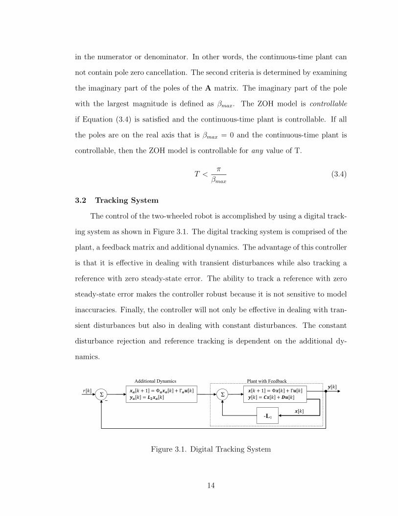
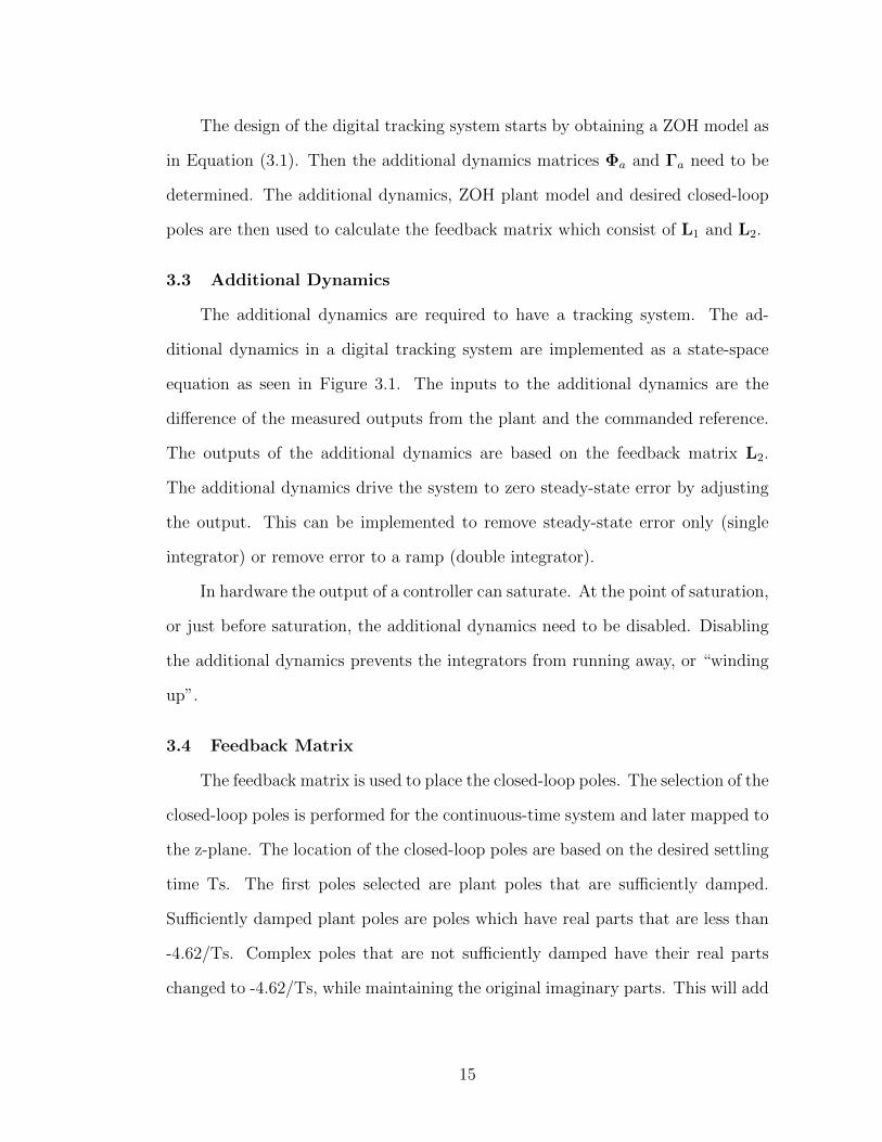
3.2 Tracking System

The control of the two-wheeled robot is accomplished by using a digital track-

ing system as shown in Figure 3.1. The digital tracking system is comprised of the

plant, a feedback matrix and additional dynamics. The advantage of this controller

is that it is effective in dealing with transient disturbances while also tracking a

reference with zero steady-state error. The ability to track a reference with zero

steady-state error makes the controller robust because it is not sensitive to model

inaccuracies. Finally, the controller will not only be effective in dealing with tran-

sient disturbances but also in dealing with constant disturbances. The constant

disturbance rejection and reference tracking is dependent on the additional dy-

namics.

[ ] [ ] [ ]

[ ] [ ] [ ]

[ ] [ ] [ ]

[ ] [ ]

Σ Σ

-L1

Additional Dynamics

Plant with Feedback

[ ]

[ ]

[ ]

-

Figure 3.1. Digital Tracking System

14

The design of the digital tracking system starts by obtaining a ZOH model as

in Equation (3.1). Then the additional dynamics matrices Φa and Γa need to be

determined. The additional dynamics, ZOH plant model and desired closed-loop

poles are then used to calculate the feedback matrix which consist of L1 and L2.

3.3 Additional Dynamics

The additional dynamics are required to have a tracking system. The ad-

ditional dynamics in a digital tracking system are implemented as a state-space

equation as seen in Figure 3.1. The inputs to the additional dynamics are the

difference of the measured outputs from the plant and the commanded reference.

The outputs of the additional dynamics are based on the feedback matrix L2.

The additional dynamics drive the system to zero steady-state error by adjusting

the output. This can be implemented to remove steady-state error only (single

integrator) or remove error to a ramp (double integrator).

In hardware the output of a controller can saturate. At the point of saturation,

or just before saturation, the additional dynamics need to be disabled. Disabling

the additional dynamics prevents the integrators from running away, or “winding

up”.

3.4 Feedback Matrix

The feedback matrix is used to place the closed-loop poles. The selection of the

closed-loop poles is performed for the continuous-time system and later mapped to

the z-plane. The location of the closed-loop poles are based on the desired settling

time Ts. The first poles selected are plant poles that are sufficiently damped.

Sufficiently damped plant poles are poles which have real parts that are less than

-4.62/Ts. Complex poles that are not sufficiently damped have their real parts

changed to -4.62/Ts, while maintaining the original imaginary parts. This will add

15

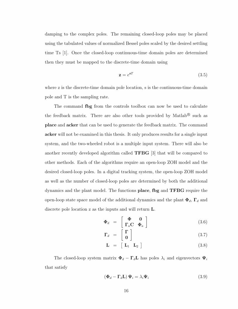
damping to the complex poles. The remaining closed-loop poles may be placed

using the tabulated values of normalized Bessel poles scaled by the desired settling

time Ts [1]. Once the closed-loop continuous-time domain poles are determined

then they must be mapped to the discrete-time domain using

z = esT (3.5)

where z is the discrete-time domain pole location, s is the continuous-time domain

pole and T is the sampling rate.

The command fbg from the controls toolbox can now be used to calculate

the feedback matrix. There are also other tools provided by Matlab R© such as

place and acker that can be used to generate the feedback matrix. The command

acker will not be examined in this thesis. It only produces results for a single input

system, and the two-wheeled robot is a multiple input system. There will also be

another recently developed algorithm called TFBG [3] that will be compared to

other methods. Each of the algorithms require an open-loop ZOH model and the

desired closed-loop poles. In a digital tracking system, the open-loop ZOH model

as well as the number of closed-loop poles are determined by both the additional

dynamics and the plant model. The functions place, fbg and TFBG require the

open-loop state space model of the additional dynamics and the plant Φd, Γd and

discrete pole location z as the inputs and will return L.

Φd =

[Φ 0

ΓaC Φa

](3.6)

Γd =

[Γ0

](3.7)

L =[

L1 L2

](3.8)

The closed-loop system matrix Φd − ΓdL has poles λi and eigenvectors Ψi

that satisfy

(Φd − ΓdL) Ψi = λiΨi (3.9)

16

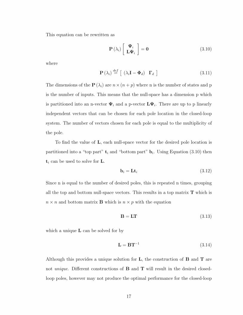
This equation can be rewritten as

P (λi)

[Ψi

LΨi

]= 0 (3.10)

where

P (λi)def=[

(λiI−Φd) Γd

](3.11)

The dimensions of the P (λi) are n× (n+ p) where n is the number of states and p

is the number of inputs. This means that the null-space has a dimension p which

is partitioned into an n-vector Ψi and a p-vector LΨi. There are up to p linearly

independent vectors that can be chosen for each pole location in the closed-loop

system. The number of vectors chosen for each pole is equal to the multiplicity of

the pole.

To find the value of L, each null-space vector for the desired pole location is

partitioned into a “top part” ti and “bottom part” bi. Using Equation (3.10) then

ti can be used to solve for L.

bi = Lti (3.12)

Since n is equal to the number of desired poles, this is repeated n times, grouping

all the top and bottom null-space vectors. This results in a top matrix T which is

n× n and bottom matrix B which is n× p with the equation

B = LT (3.13)

which a unique L can be solved for by

L = BT−1 (3.14)

Although this provides a unique solution for L, the construction of B and T are

not unique. Different constructions of B and T will result in the desired closed-

loop poles, however may not produce the optimal performance for the closed-loop

17

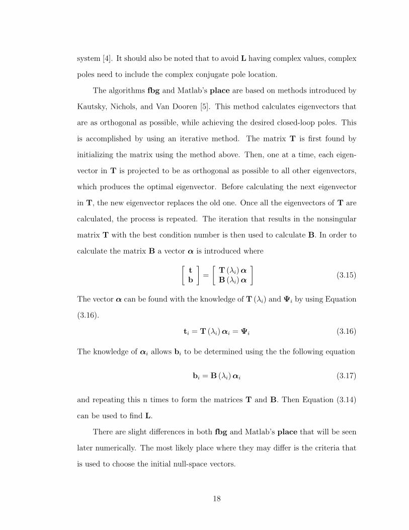
system [4]. It should also be noted that to avoid L having complex values, complex

poles need to include the complex conjugate pole location.

The algorithms fbg and Matlab’s place are based on methods introduced by

Kautsky, Nichols, and Van Dooren [5]. This method calculates eigenvectors that

are as orthogonal as possible, while achieving the desired closed-loop poles. This

is accomplished by using an iterative method. The matrix T is first found by

initializing the matrix using the method above. Then, one at a time, each eigen-

vector in T is projected to be as orthogonal as possible to all other eigenvectors,

which produces the optimal eigenvector. Before calculating the next eigenvector

in T, the new eigenvector replaces the old one. Once all the eigenvectors of T are

calculated, the process is repeated. The iteration that results in the nonsingular

matrix T with the best condition number is then used to calculate B. In order to

calculate the matrix B a vector α is introduced where[tb

]=

[T (λi)αB (λi)α

](3.15)

The vector α can be found with the knowledge of T (λi) and Ψi by using Equation

(3.16).

ti = T (λi)αi = Ψi (3.16)

The knowledge of αi allows bi to be determined using the the following equation

bi = B (λi)αi (3.17)

and repeating this n times to form the matrices T and B. Then Equation (3.14)

can be used to find L.

There are slight differences in both fbg and Matlab’s place that will be seen

later numerically. The most likely place where they may differ is the criteria that

is used to choose the initial null-space vectors.

18

The new method of calculating L is based on optimizing a stability robustness

norm, which is described in Burl [6]. The calculation of L is performed in the

function TFBG. TFBG is initialized using the same method as fbg, which is

the only commonality between the two algorithms. The new algorithm searches

for stability robustness in a system with a MIMO plant. The stability robustness

indicates how big ∆(z), the error in the plant, can be before the system goes

unstable, where I + ∆(z) is a MIMO transfer function cascaded with the plant.

The inputs and outputs of ∆(z) are yd and wd respectively, and if ∆(z) = 0 then

the control system is using the nominal plant model. The condition for stability

of the control system is

‖∆(z)N(z)‖∞ < 1 (3.18)

where N(z) is the transfer function from wd to yd. Using the relationship

‖∆(z)N(z)‖∞ ≤ ‖∆(z)‖∞ ‖N(z)‖∞ < 1 (3.19)

the robustness norm δmax can be found by

‖∆(z)N(z)‖∞ <1

‖N(z)‖∞(3.20)

δmax =1

‖N(z)‖∞

The objective of TFBG is to find L that results in the largest possible δmax. The

two-wheeled robot requires another constraint, where the rows of L have the same

magnitude and certain columns have opposite signs.

3.5 Stability Margins

The value of δmax is directly related to the gain and phase margin of the

control system. In a SISO system the stability margins can be found using q, which

represents gain and phase uncertainty of the plant in classical control. In a MIMO

system q could be used; however the stability margins are only representative of the

19

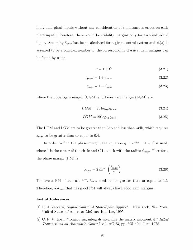
individual plant inputs without any consideration of simultaneous errors on each

plant input. Therefore, there would be stability margins only for each individual

input. Assuming δmax has been calculated for a given control system and ∆(z) is

assumed to be a complex number C, the corresponding classical gain margins can

be found by using

q = 1 + C (3.21)

qmax = 1 + δmax (3.22)

qmin = 1− δmax (3.23)

where the upper gain margin (UGM) and lower gain margin (LGM) are

UGM = 20 log10 qmax (3.24)

LGM = 20 log10 qmin (3.25)

The UGM and LGM are to be greater than 3db and less than -3db, which requires

δmax to be greater than or equal to 0.4.

In order to find the phase margin, the equation q = e−jφ = 1 + C is used,

where 1 is the center of the circle and C is a disk with the radius δmax. Therefore,

the phase margin (PM) is

φmax = 2 sin−1

(δmax

2

)(3.26)

To have a PM of at least 30, δmax needs to be greater than or equal to 0.5.

Therefore, a δmax that has good PM will always have good gain margins.

List of References


[2] C. F. V. Loan, “Computing integrals involving the matrix exponential,” IEEETransactions on Automatic Control, vol. AC-23, pp. 395–404, June 1978.

20

[3] R. J. Vaccaro, Department of Electrical, Computer, and Biomedical Engineer-ing, University of Rhode Island, Kingston RI 02881, United States of America,October 2011, personal communication.

[4] V. Sima, A. L. Tits, and Y. Yang, “Computational experience with robustpole assignment algorithms,” Conference on Computer Aided Control SystemsDesign, vol. WeA01.6, pp. 36–41, October 2006.

[5] J. Kautsky, N. Nichols, and P. V. Dooren, “Robust pole assignment in linearstate feedback,” International Journal of Control, vol. 41, pp. 1129–1155, 1985.

[6] J. B. Burl, Linear Optimal Control. Reading, Massachusetts, United Statesof America: Addison-Wesley, 1998.

21

CHAPTER 4

Hardware

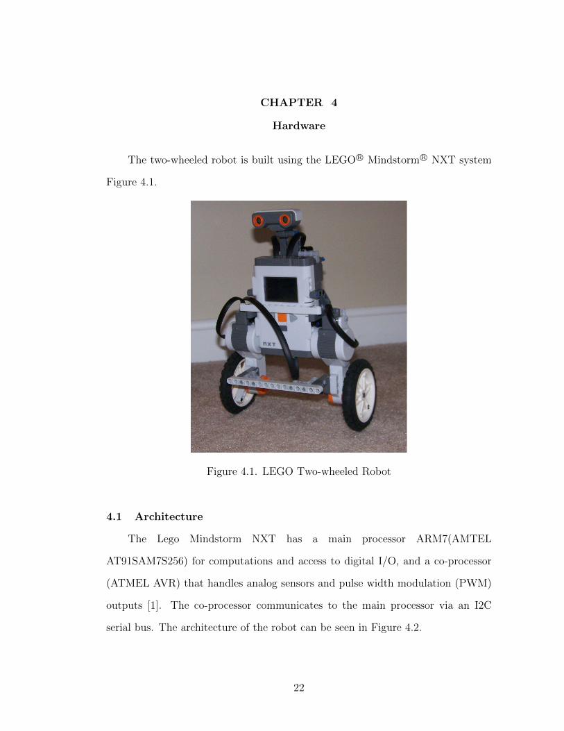
The two-wheeled robot is built using the LEGO R© Mindstorm R© NXT system

Figure 4.1.

Figure 4.1. LEGO Two-wheeled Robot

4.1 Architecture

The Lego Mindstorm NXT has a main processor ARM7(AMTEL

AT91SAM7S256) for computations and access to digital I/O, and a co-processor

(ATMEL AVR) that handles analog sensors and pulse width modulation (PWM)

outputs [1]. The co-processor communicates to the main processor via an I2C

serial bus. The architecture of the robot can be seen in Figure 4.2.

22

AMTEL

AT91SAM7S256

ATMEL AVR

I2C

C B

Right Motor

3

Left Motor

PWMr PWMl

Gyro

Encoderr Encoderl

PC with GUI

Figure 4.2. Hardware Architecture

There are three sensors and two actuators that are used in the system. The

motors receive their PWM commands from the co-processor and the encoder feed-

back is sent directly to the main processor. The voltages that are applied to each

motor range from plus or minus the battery voltage. The encoders for each motor

contain 360 counts per revolution and have a resolution of 0.0175 rad/count. The

HiTechnic R© Gyro Sensor is a single axis gyroscopic sensor. The axis of measure-

ment is shown in Figure 4.3. It can detect angular speed at a resolution of 0.0175

rad/sec. The Gyro is an analog sensor and so it utilizes the co-processor. The

data from the AVR is accessed every 2 ms. The PWM commands are sent for 1

ms and the sensor feedback is received the next 1 ms.

23

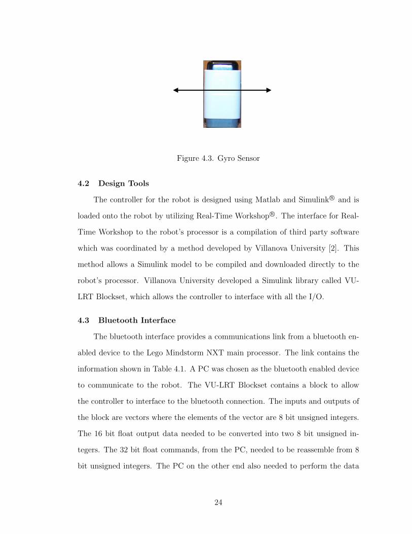
Figure 4.3. Gyro Sensor

4.2 Design Tools

The controller for the robot is designed using Matlab and Simulink R© and is

loaded onto the robot by utilizing Real-Time Workshop R©. The interface for Real-

Time Workshop to the robot’s processor is a compilation of third party software

which was coordinated by a method developed by Villanova University [2]. This

method allows a Simulink model to be compiled and downloaded directly to the

robot’s processor. Villanova University developed a Simulink library called VU-

LRT Blockset, which allows the controller to interface with all the I/O.

4.3 Bluetooth Interface

The bluetooth interface provides a communications link from a bluetooth en-

abled device to the Lego Mindstorm NXT main processor. The link contains the

information shown in Table 4.1. A PC was chosen as the bluetooth enabled device

to communicate to the robot. The VU-LRT Blockset contains a block to allow

the controller to interface to the bluetooth connection. The inputs and outputs of

the block are vectors where the elements of the vector are 8 bit unsigned integers.

The 16 bit float output data needed to be converted into two 8 bit unsigned in-

tegers. The 32 bit float commands, from the PC, needed to be reassemble from 8

bit unsigned integers. The PC on the other end also needed to perform the data

24

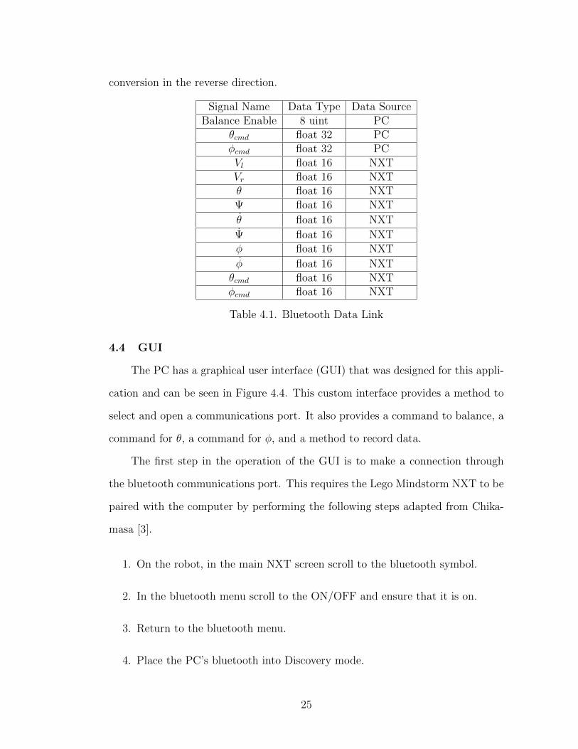
conversion in the reverse direction.

Signal Name Data Type Data SourceBalance Enable 8 uint PC

θcmd float 32 PCφcmd float 32 PCVl float 16 NXTVr float 16 NXTθ float 16 NXTΨ float 16 NXT

θ float 16 NXT

Ψ float 16 NXTφ float 16 NXT

φ float 16 NXTθcmd float 16 NXTφcmd float 16 NXT

Table 4.1. Bluetooth Data Link

4.4 GUI

The PC has a graphical user interface (GUI) that was designed for this appli-

cation and can be seen in Figure 4.4. This custom interface provides a method to

select and open a communications port. It also provides a command to balance, a

command for θ, a command for φ, and a method to record data.

The first step in the operation of the GUI is to make a connection through

the bluetooth communications port. This requires the Lego Mindstorm NXT to be

paired with the computer by performing the following steps adapted from Chika-

masa [3].

1. On the robot, in the main NXT screen scroll to the bluetooth symbol.

2. In the bluetooth menu scroll to the ON/OFF and ensure that it is on.

3. Return to the bluetooth menu.

4. Place the PC’s bluetooth into Discovery mode.

25

5. In the NXT bluetooth menu scroll and select search, then select the PC that

the NXT should be paired to.

6. The NXT will provide a pairing number and once that number is accepted

it will attempt to connect to the PC.

7. The PC should indicate that the NXT is trying to connect and requires the

pairing number. Provide the number and finalize the connection.

8. Then to determine what communications port will be used, go to the blue-

tooth settings on th PC and locate the port associated with “outgoing NXT

’Dev B”’.

Figure 4.4. Control GUI

The communications port that was found using the pairing method used above

is the port selection used in the GUI. This port will remain the link to the Lego

Mindstorm NXT until the device is removed from the PC. Now that the bluetooth

is configured, the GUI can be used to control the robot. The following steps are

taken to run the robot and assume that the controller with the bluetooth interface

block has been preloaded.

26

1. Turn on the Lego Mindstorm NXT and press the orange button until the

nxtOSEK screen flashes.

2. Select “Run” by pressing the right arrow. The robot will beep once the

calibration of the Gyro is complete. The robot should not be moved prior to

the beep since this will result in an abnormal gyro calibration.

3. Run the GUI in Matlab.

4. In the drop down menu, select the communications port for the bluetooth

interface.

5. Click on “Connect”. Once a connection is made the “Balance” button will

activate.

6. Place the robot in an upright position on a surface and press the “Balance”

button. Once the robot starts to balance, let go and let the controller do the

work.

7. In the test panel, select from the four tests that can be performed.

8. Clicking “Start” will send the profile and collect data. Once the profile is

finished, the data is available in Trial.mat.

4.5 Controller Design Considerations

The main processor is a 32 bit fixed point processor. The Real-Time Workshop

allows floating point calculations to to be performed on the 32 bit fixed point

processor. These operations will consume more processing time. The controller

will be implemented in floating point; therefore, the extra computation is a factor.

The data that will be sent back and forth over bluetooth communications also

requires processing time. These factors determined that a 10ms sampling interval

27

should be used. The high sampling interval is also much higher than the interval

at which the I2C communications are handled with the AVR. Therefore, the I2C

delays will not be a factor in the design and analysis of the controller.

The hardware will also affect the design of the controller since the resolution

of the sensors is low. This requires the controller to have a slower setting time so

that the controller does not respond to the bit changes. This affects the system

most when it is trying to balance in place and a bit change occurs causing a large

derivative. A slower settling time means the gains are not tuned so high that the

large derivative cause the voltage inputs to saturate. There are other effects such

as the sloppy gears that produce dead bands and the saturation point of the output

at the battery voltage that requires slower settling times.

List of References

[1] T. Chikamasa, “Embedded coder robot nxt mod-eling tips,” April 2010, unpublished. [Online].Available: http://www.mathworks.com/matlabcentral/fileexchange/13399-embedded-coder-robot-nxt-demo?controller=file infos&download=true

[2] J. P. Jones, C. McArthur, and T. Young, VU-LEGO Real Time Target: User’sGuide, 1st ed., Center for Nonlinear Dynamics and Control, Villanova Univer-sity, Villanova PA 19085, United States of America, February 2011.

[3] T. Chikamasa, “Nxt gamepad,” January 2009, unpublished. [Online].Available: http://lejos-osek.sourceforge.net/nxtgamepad.htm

28



http://lejos-osek.sourceforge.net/nxtgamepad.htm

CHAPTER 5

Controller Design

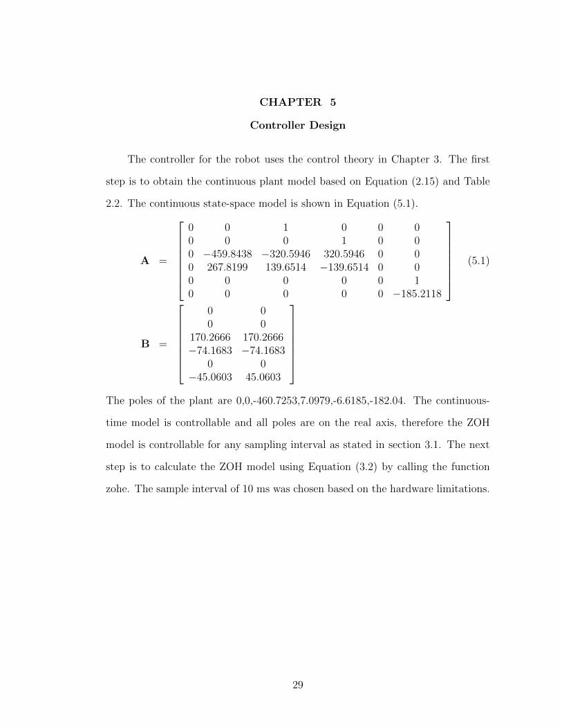
The controller for the robot uses the control theory in Chapter 3. The first

step is to obtain the continuous plant model based on Equation (2.15) and Table

2.2. The continuous state-space model is shown in Equation (5.1).

A =

0 0 1 0 0 00 0 0 1 0 00 −459.8438 −320.5946 320.5946 0 00 267.8199 139.6514 −139.6514 0 00 0 0 0 0 10 0 0 0 0 −185.2118

(5.1)

B =

0 00 0

170.2666 170.2666−74.1683 −74.1683

0 0−45.0603 45.0603

The poles of the plant are 0,0,-460.7253,7.0979,-6.6185,-182.04. The continuous-

time model is controllable and all poles are on the real axis, therefore the ZOH

model is controllable for any sampling interval as stated in section 3.1. The next

step is to calculate the ZOH model using Equation (3.2) by calling the function

zohe. The sample interval of 10 ms was chosen based on the hardware limitations.

29

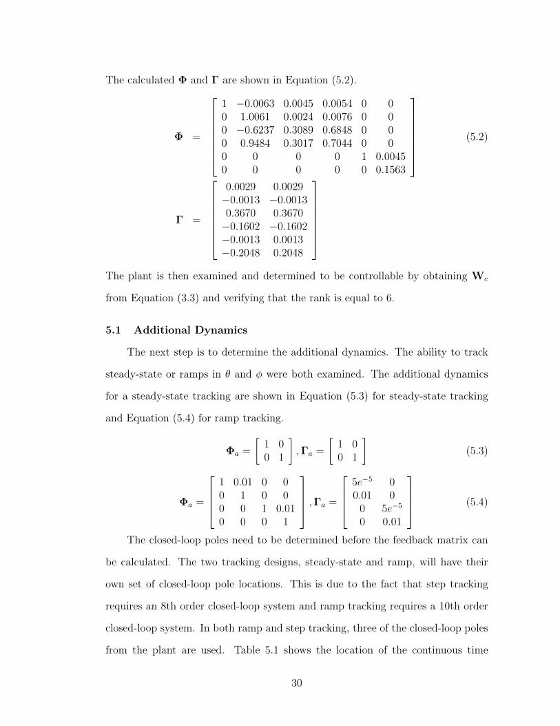
The calculated Φ and Γ are shown in Equation (5.2).

Φ =

1 −0.0063 0.0045 0.0054 0 00 1.0061 0.0024 0.0076 0 00 −0.6237 0.3089 0.6848 0 00 0.9484 0.3017 0.7044 0 00 0 0 0 1 0.00450 0 0 0 0 0.1563

(5.2)

Γ =

0.0029 0.0029−0.0013 −0.00130.3670 0.3670−0.1602 −0.1602−0.0013 0.0013−0.2048 0.2048

The plant is then examined and determined to be controllable by obtaining Wc

from Equation (3.3) and verifying that the rank is equal to 6.

5.1 Additional Dynamics

The next step is to determine the additional dynamics. The ability to track

steady-state or ramps in θ and φ were both examined. The additional dynamics

for a steady-state tracking are shown in Equation (5.3) for steady-state tracking

and Equation (5.4) for ramp tracking.

Φa =

[1 00 1

],Γa =

[1 00 1

](5.3)

Φa =

1 0.01 0 00 1 0 00 0 1 0.010 0 0 1

,Γa =

5e−5 00.01 0

0 5e−5

0 0.01

(5.4)

The closed-loop poles need to be determined before the feedback matrix can

be calculated. The two tracking designs, steady-state and ramp, will have their

own set of closed-loop pole locations. This is due to the fact that step tracking

requires an 8th order closed-loop system and ramp tracking requires a 10th order

closed-loop system. In both ramp and step tracking, three of the closed-loop poles

from the plant are used. Table 5.1 shows the location of the continuous time

30

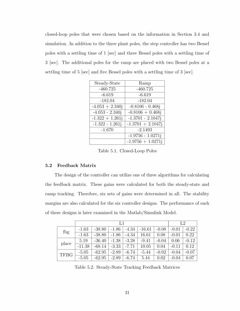
closed-loop poles that were chosen based on the information in Section 3.4 and

simulation. In addition to the three plant poles, the step controller has two Bessel

poles with a settling time of 1 [sec] and three Bessel poles with a settling time of

3 [sec]. The additional poles for the ramp are placed with two Bessel poles at a

settling time of 5 [sec] and five Bessel poles with a settling time of 3 [sec].

Steady-State Ramp-460.725 -460.725-6.619 -6.619-182.04 -182.04

-4.053 + 2.340j -0.8106 - 0.468j-4.053 - 2.340j -0.8106 + 0.468j-1.322 + 1.261j -1.3701 - 2.1047j-1.322 - 1.261j -1.3701 + 2.1047j

-1.670 -2.1493-1.9756 - 1.0271j-1.9756 + 1.0271j

Table 5.1. Closed-Loop Poles

5.2 Feedback Matrix

The design of the controller can utilize one of three algorithms for calculating

the feedback matrix. These gains were calculated for both the steady-state and

ramp tracking. Therefore, six sets of gains were determined in all. The stability

margins are also calculated for the six controller designs. The performance of each

of these designs is later examined in the Matlab/Simulink Model.

L1 L2

fbg-1.63 -38.80 -1.86 -4.34 -16.61 -0.08 -0.01 -0.22-1.63 -38.80 -1.86 -4.34 16.61 0.08 -0.01 0.22

place5.19 -36.40 -1.38 -3.28 -9.41 -0.04 0.06 -0.12

-11.38 -68.14 -3.33 -7.71 10.05 0.04 -0.11 0.12

TFBG-5.05 -62.95 -2.89 -6.74 -5.44 -0.02 -0.04 -0.07-5.05 -62.95 -2.89 -6.74 5.44 0.02 -0.04 0.07

Table 5.2. Steady-State Tracking Feedback Matrices

31

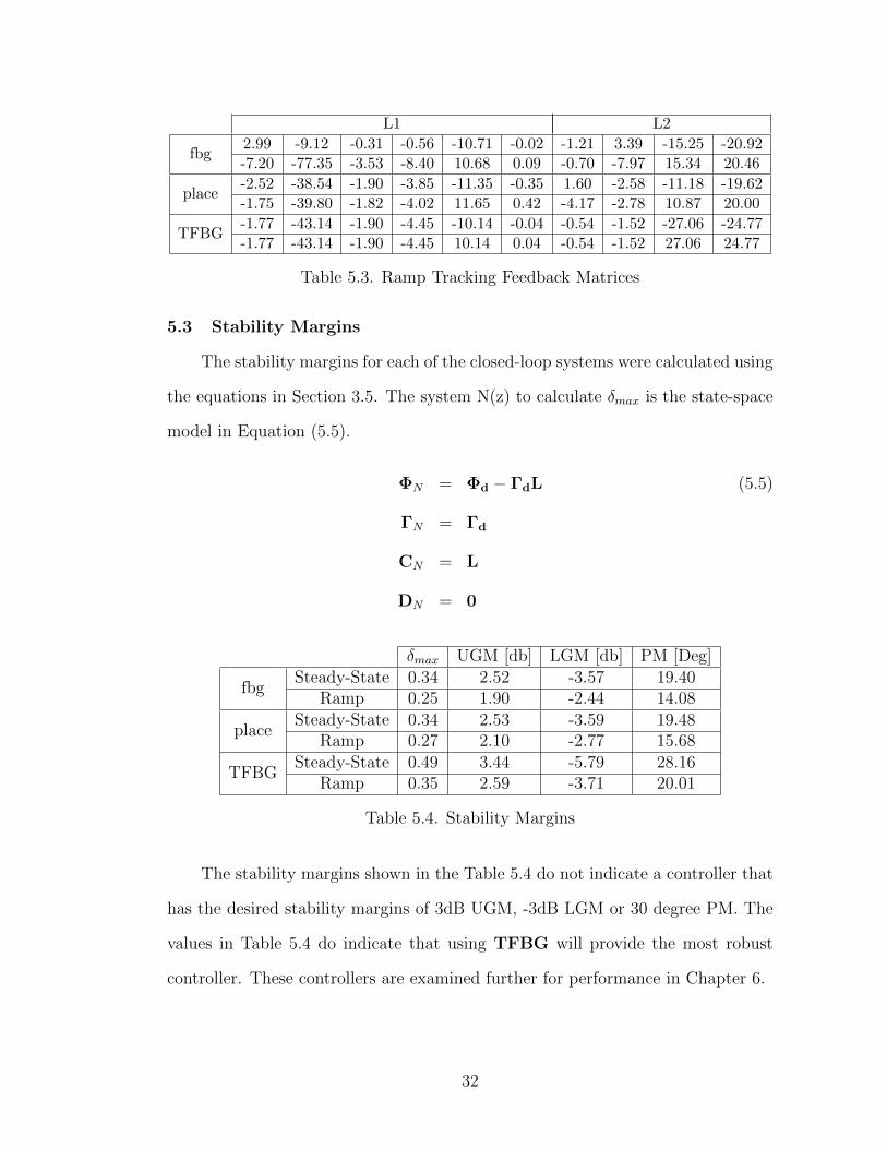
L1 L2

fbg2.99 -9.12 -0.31 -0.56 -10.71 -0.02 -1.21 3.39 -15.25 -20.92-7.20 -77.35 -3.53 -8.40 10.68 0.09 -0.70 -7.97 15.34 20.46

place-2.52 -38.54 -1.90 -3.85 -11.35 -0.35 1.60 -2.58 -11.18 -19.62-1.75 -39.80 -1.82 -4.02 11.65 0.42 -4.17 -2.78 10.87 20.00

TFBG-1.77 -43.14 -1.90 -4.45 -10.14 -0.04 -0.54 -1.52 -27.06 -24.77-1.77 -43.14 -1.90 -4.45 10.14 0.04 -0.54 -1.52 27.06 24.77

Table 5.3. Ramp Tracking Feedback Matrices

5.3 Stability Margins

The stability margins for each of the closed-loop systems were calculated using

the equations in Section 3.5. The system N(z) to calculate δmax is the state-space

model in Equation (5.5).

ΦN = Φd − ΓdL (5.5)

ΓN = Γd

CN = L

DN = 0

δmax UGM [db] LGM [db] PM [Deg]

fbgSteady-State 0.34 2.52 -3.57 19.40

Ramp 0.25 1.90 -2.44 14.08

placeSteady-State 0.34 2.53 -3.59 19.48

Ramp 0.27 2.10 -2.77 15.68

TFBGSteady-State 0.49 3.44 -5.79 28.16

Ramp 0.35 2.59 -3.71 20.01

Table 5.4. Stability Margins

The stability margins shown in the Table 5.4 do not indicate a controller that

has the desired stability margins of 3dB UGM, -3dB LGM or 30 degree PM. The

values in Table 5.4 do indicate that using TFBG will provide the most robust

controller. These controllers are examined further for performance in Chapter 6.

32

5.4 Plant Inputs and Outputs

In order to implement the controller, the feedback and commands of the robot

need to be transformed into the states that are shown in Equation (2.14). The

feedback signals from the robot are θml, θmr

and Ψ which are converted from

degrees to radians and then used to find the required states. θ and φ are determined

by using Equations (2.1) and (2.2). Ψ is calculated by using a forward Euler

integration of Ψ.

Ψ[k + 1] = Ψ[k] + T Ψ[k] (5.6)

The state variables φ and θ require the derivative of θ and φ. The derivative

was implemented as a second order filter with a specific settling time in order

to reject any frequencies that are higher than the system response. The filter is

designed using Bessel roots with a settling time of 0.025 [sec] which results in the

transfer function in Equation(5.7).

H(s) =35044s

s2 + 324.24s+ 35044(5.7)

Converting the transfer function to a continuous state-space model and then using

the zohe command with a sampling time of 0.01 [sec] generates the discrete state-

space Equation (5.8) for the filtered derivative.

x[k + 1] = Φfx[k] + Γfu[k] (5.8)

y[k] = Cfx[k]

Φf =

[0.3928 0.0017−59.588 −0.1585

]Γf =

[0.60759.59

]Cf =

[0 1

]Estimates of the state variables φ and θ could have been implemented using a

linear observer system. However, modeling has shown that non-linearities due to

quantization make it difficult to use the linear observer accurately.

33

The outputs of the plant require scaling. Since the DC motor voltage is PWM

based, the voltage from the controller is scaled and limited by the battery voltage

(±Vbat). The commands sent to the motors are PWMl,r = 100(Vl,rVbat

). The presence

of the limiters require that the additional dynamics, which are integrators, be held

in order to keep them from rapidly growing while in the limits. The integrators are

not held exactly at ±Vbat but at a voltage slightly lower. Limiting the integrators

at a lower voltage than the battery allows the controller to respond as a regulator

for the remaining voltage head room. The regulator is the main component used

to maintain the robot’s balance, giving a priority to the system, which is first

balancing and second maneuvering.

34

CHAPTER 6

Modeling and Simulations

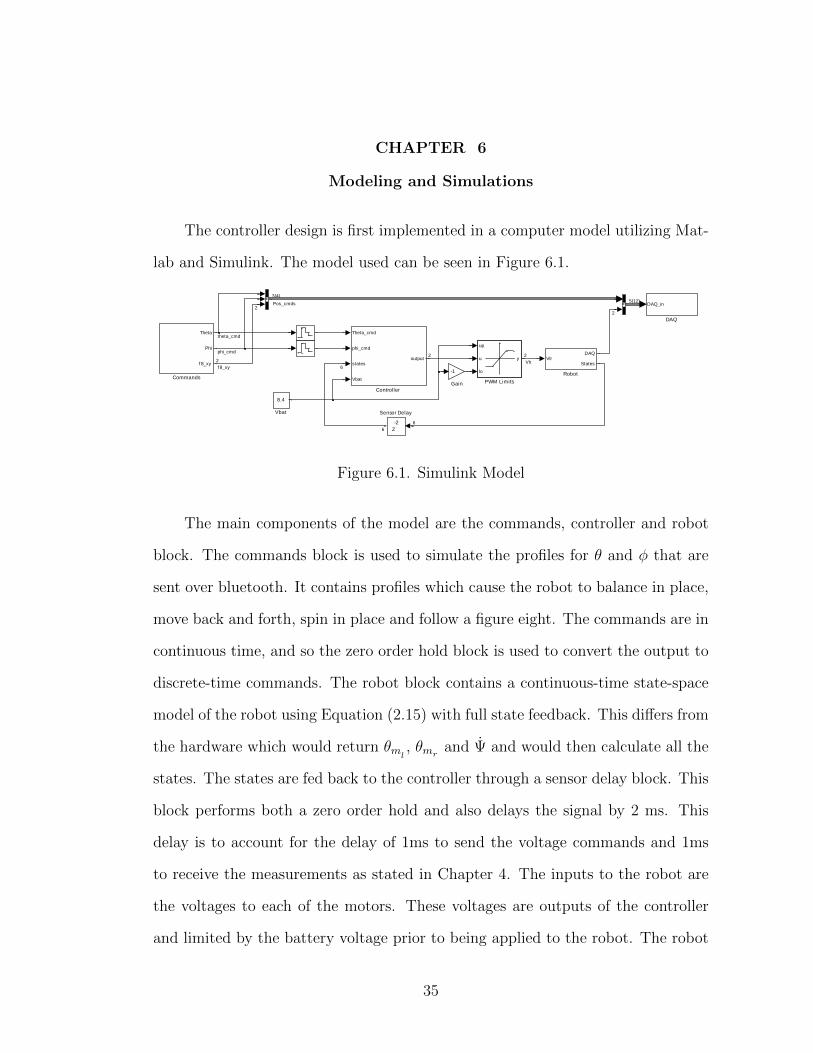
The controller design is first implemented in a computer model utilizing Mat-

lab and Simulink. The model used can be seen in Figure 6.1.

8.4

Vbat

-2

Z

Sensor Delay

VlrDAQ

States

Robot

up

u

lo

y

PWM Limits

-1

Gain

DAQ_in

DAQ

Theta_cmd

phi_cmd

states

Vbat

output

Controller

Theta

Phi

f 8_xy

Commands

theta_cmd

phi_cmd

2

2

f 8_xy

6

6

2 2

Vlr

34

Pos_cmds 512

2

6

Figure 6.1. Simulink Model

The main components of the model are the commands, controller and robot

block. The commands block is used to simulate the profiles for θ and φ that are

sent over bluetooth. It contains profiles which cause the robot to balance in place,

move back and forth, spin in place and follow a figure eight. The commands are in

continuous time, and so the zero order hold block is used to convert the output to

discrete-time commands. The robot block contains a continuous-time state-space

model of the robot using Equation (2.15) with full state feedback. This differs from

the hardware which would return θml, θmr

and Ψ and would then calculate all the

states. The states are fed back to the controller through a sensor delay block. This

block performs both a zero order hold and also delays the signal by 2 ms. This

delay is to account for the delay of 1ms to send the voltage commands and 1ms

to receive the measurements as stated in Chapter 4. The inputs to the robot are

the voltages to each of the motors. These voltages are outputs of the controller

and limited by the battery voltage prior to being applied to the robot. The robot

35

voltage inputs and states along with the commands are sent to the DAQ block so

that data can be collected and analyzed.

The final block is the controller. This block contains most of the controller

that was designed in Chapter 5 and is shown in Figure 6.2.

output

1

Outputs

c* u

Integrator Hold

batt

VcmdInibit

-L1* u

doublesingle

single

Additional Dynamics

In1 Out1

Vbat

4

states

3

phi_cmd

2

Theta_cmd

1

2

2

2

6

2

2

2

2

2

6

6

6

2 222

Figure 6.2. Controller

The additional dynamics block is implemented using a discrete state-space

equation with the values calculated in Chapter 5 for Φa, Γa and L2. The input to

the additional dynamics block is the error of the commanded and measured θ and φ.

The additional dynamics block is only enabled when the motor voltage commands

are between ± 95% of Vbat. The output of the controller is the subtraction of the

voltages of state feedback gain L1 and the voltages of the additional dynamics.

The parameters needed for both the simulation and the control design are

produced in files Parameters.m and Controller.m included in the Appendix. The

model will automatically call the files when the model is opened and every time

the model is started.

6.1 Performance Testing

The model was used to determine the performance of the controller design for

each of the feedback matrix calculation algorithms to both steady-state and ramp

tracking. In Chapter 5 the stability margins for each feedback matrix calculation

algorithm with steady-state and ramp tracking were calculated. The stability

36

margins are a good indication of how the design will perform. However, even

though the stability margins may show the system to be more robust, the dynamics

may still not produce the best performance.

Steady-State Tracking

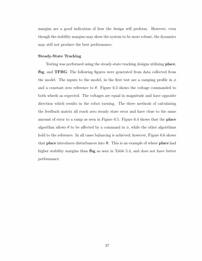
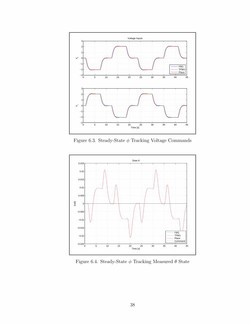
Testing was performed using the steady-state tracking designs utilizing place,

fbg, and TFBG. The following figures were generated from data collected from

the model. The inputs to the model, in the first test are a ramping profile in φ

and a constant zero reference to θ. Figure 6.3 shows the voltage commanded to

both wheels as expected. The voltages are equal in magnitude and have opposite

direction which results in the robot turning. The three methods of calculating

the feedback matrix all reach zero steady state error and have close to the same

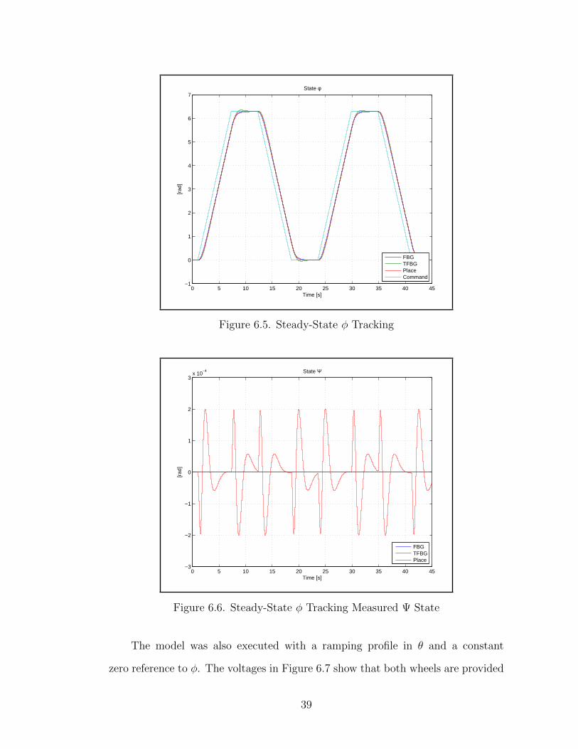
amount of error to a ramp as seen in Figure 6.5. Figure 6.4 shows that the place

algorithm allows θ to be affected by a command in φ, while the other algorithms

hold to the reference. In all cases balancing is achieved; however, Figure 6.6 shows

that place introduces disturbances into Ψ. This is an example of where place had

higher stability margins than fbg as seen in Table 5.4, and does not have better

performance.

37

0 5 10 15 20 25 30 35 40 45−3

−2

−1

0

1

2

3

Vl

Voltage Inputs

FBGTFBGPlace

0 5 10 15 20 25 30 35 40 45−3

−2

−1

0

1

2

3

Vr

Time [s]

Figure 6.3. Steady-State φ Tracking Voltage Commands

0 5 10 15 20 25 30 35 40 45−0.025

−0.02

−0.015

−0.01

−0.005

0

0.005

0.01

0.015

0.02

0.025

Time [s]

[rad

]

State θ

FBGTFBGPlaceCommand

Figure 6.4. Steady-State φ Tracking Measured θ State

38

0 5 10 15 20 25 30 35 40 45−1

0

1

2

3

4

5

6

7

Time [s]

[rad

]

State φ

FBGTFBGPlaceCommand

Figure 6.5. Steady-State φ Tracking

0 5 10 15 20 25 30 35 40 45−3

−2

−1

0

1

2

3x 10

−4

Time [s]

[rad

]

State Ψ

FBGTFBGPlace

Figure 6.6. Steady-State φ Tracking Measured Ψ State

The model was also executed with a ramping profile in θ and a constant

zero reference to φ. The voltages in Figure 6.7 show that both wheels are provided

39

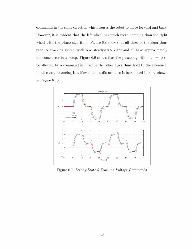
commands in the same direction which causes the robot to move forward and back.

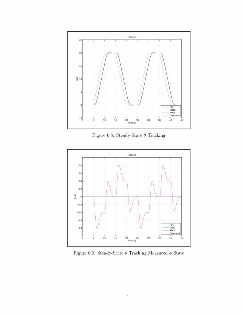
However, it is evident that the left wheel has much more damping than the right

wheel with the place algorithm. Figure 6.8 show that all three of the algorithms

produce tracking system with zero steady-state error and all have approximately

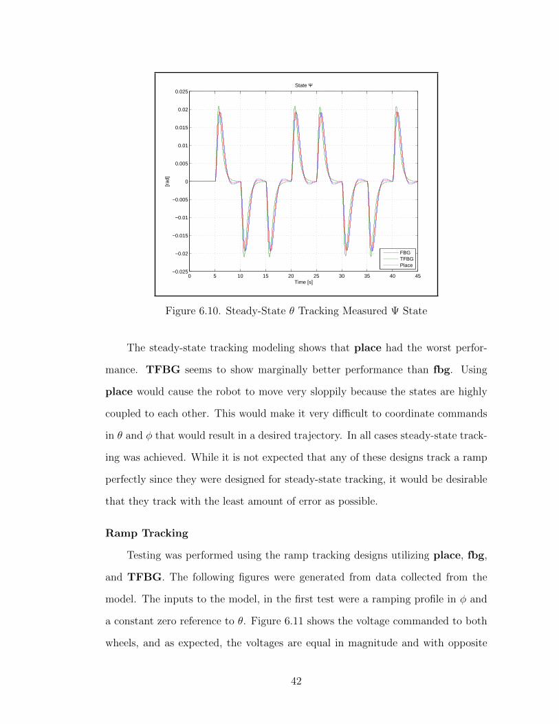
the same error to a ramp. Figure 6.9 shows that the place algorithm allows φ to

be affected by a command in θ, while the other algorithms hold to the reference.

In all cases, balancing is achieved and a disturbance is introduced in Ψ as shown

in Figure 6.10.

0 5 10 15 20 25 30 35 40 45−4

−2

0

2

4

Vl

Voltage Inputs

FBGTFBGPlace

0 5 10 15 20 25 30 35 40 45−6

−4

−2

0

2

4

6

Vr

Time [s]

Figure 6.7. Steady-State θ Tracking Voltage Commands

40

0 5 10 15 20 25 30 35 40 45−5

0

5

10

15

20

25

Time [s]

[rad

]

State θ

FBGTFBGPlaceCommand

Figure 6.8. Steady-State θ Tracking

0 5 10 15 20 25 30 35 40 45−1

−0.8

−0.6

−0.4

−0.2

0

0.2

0.4

0.6

0.8

1

Time [s]

[rad

]

State φ

FBGTFBGPlaceCommand

Figure 6.9. Steady-State θ Tracking Measured φ State

41

0 5 10 15 20 25 30 35 40 45−0.025

−0.02

−0.015

−0.01

−0.005

0

0.005

0.01

0.015

0.02

0.025

Time [s]

[rad

]

State Ψ

FBGTFBGPlace

Figure 6.10. Steady-State θ Tracking Measured Ψ State

The steady-state tracking modeling shows that place had the worst perfor-

mance. TFBG seems to show marginally better performance than fbg. Using

place would cause the robot to move very sloppily because the states are highly

coupled to each other. This would make it very difficult to coordinate commands

in θ and φ that would result in a desired trajectory. In all cases steady-state track-

ing was achieved. While it is not expected that any of these designs track a ramp

perfectly since they were designed for steady-state tracking, it would be desirable

that they track with the least amount of error as possible.

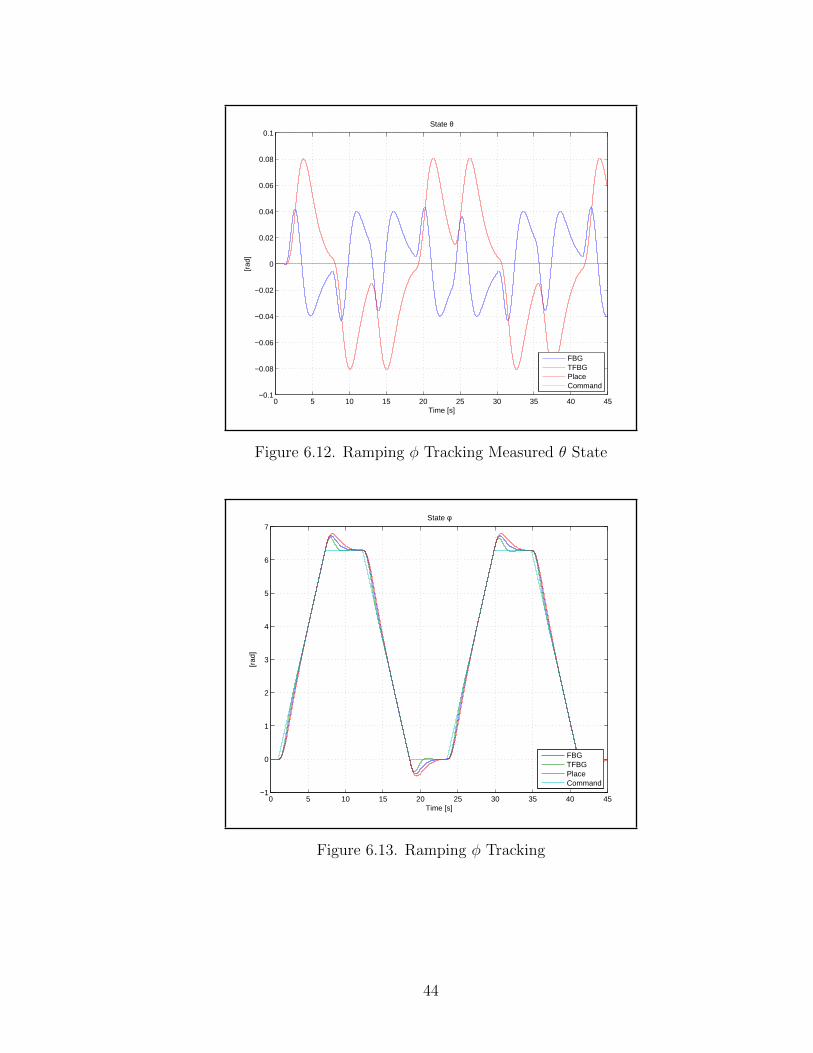
Ramp Tracking

Testing was performed using the ramp tracking designs utilizing place, fbg,

and TFBG. The following figures were generated from data collected from the

model. The inputs to the model, in the first test were a ramping profile in φ and

a constant zero reference to θ. Figure 6.11 shows the voltage commanded to both

wheels, and as expected, the voltages are equal in magnitude and with opposite

42

direction, which results in the robot turning. The voltage commands show that

the TFBG algorithm has a faster response, which can also be seen in Figure

6.13 where TFBG has less overshoot. Figure 6.12 shows that the place and fbg

algorithms allow θ to be affected by a command in φ, while the TFBG algorithm

hold to the reference. In all cases balancing is achieved. However, Figure 6.14

shows that place and fbg introduces disturbances into Ψ. In this case TFBG

from Table 5.4 has the best performance and stability margins.

0 5 10 15 20 25 30 35 40 45−3

−2

−1

0

1

2

3

Vl

Voltage Inputs

FBGTFBGPlace

0 5 10 15 20 25 30 35 40 45−3

−2

−1

0

1

2

3

Vr

Time [s]

Figure 6.11. Ramping φ Tracking Voltage Commands

43

0 5 10 15 20 25 30 35 40 45−0.1

−0.08

−0.06

−0.04

−0.02

0

0.02

0.04

0.06

0.08

0.1

Time [s]

[rad

]

State θ

FBGTFBGPlaceCommand

Figure 6.12. Ramping φ Tracking Measured θ State

0 5 10 15 20 25 30 35 40 45−1

0

1

2

3

4

5

6

7

Time [s]

[rad

]

State φ

FBGTFBGPlaceCommand

Figure 6.13. Ramping φ Tracking

44

0 5 10 15 20 25 30 35 40 45−1

−0.8

−0.6

−0.4

−0.2

0

0.2

0.4

0.6

0.8

1x 10

−3

Time [s]

[rad

]

State Ψ

FBGTFBGPlace

Figure 6.14. Ramping φ Tracking Measured Ψ State

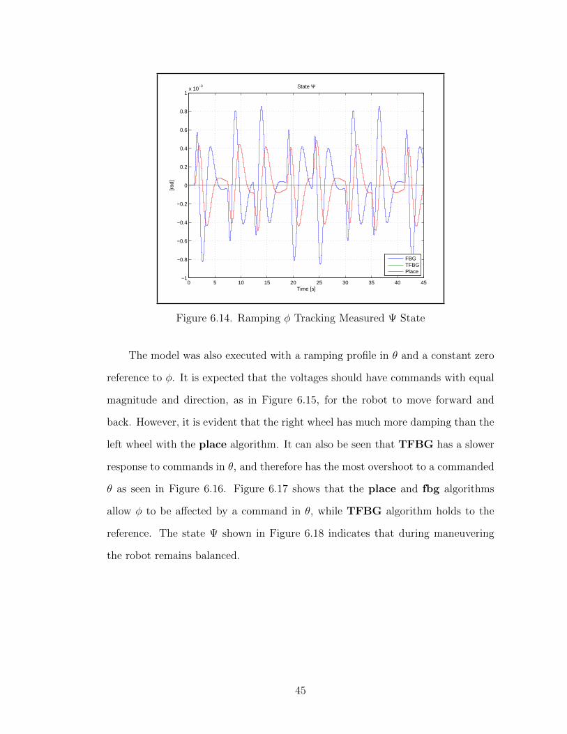
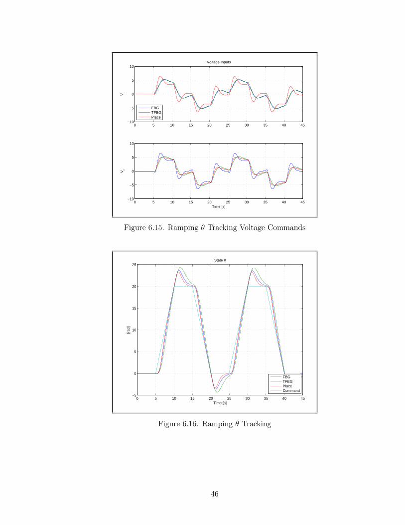
The model was also executed with a ramping profile in θ and a constant zero

reference to φ. It is expected that the voltages should have commands with equal

magnitude and direction, as in Figure 6.15, for the robot to move forward and

back. However, it is evident that the right wheel has much more damping than the

left wheel with the place algorithm. It can also be seen that TFBG has a slower

response to commands in θ, and therefore has the most overshoot to a commanded

θ as seen in Figure 6.16. Figure 6.17 shows that the place and fbg algorithms

allow φ to be affected by a command in θ, while TFBG algorithm holds to the

reference. The state Ψ shown in Figure 6.18 indicates that during maneuvering

the robot remains balanced.

45

0 5 10 15 20 25 30 35 40 45−10

−5

0

5

10

Vl

Voltage Inputs

FBGTFBGPlace

0 5 10 15 20 25 30 35 40 45−10

−5

0

5

10

Vr

Time [s]

Figure 6.15. Ramping θ Tracking Voltage Commands

0 5 10 15 20 25 30 35 40 45−5

0

5

10

15

20

25

Time [s]

[rad

]

State θ

FBGTFBGPlaceCommand

Figure 6.16. Ramping θ Tracking

46

0 5 10 15 20 25 30 35 40 45−0.8

−0.6

−0.4

−0.2

0

0.2

0.4

0.6

0.8

Time [s]

[rad

]

State φ

FBGTFBGPlaceCommand

Figure 6.17. Ramping θ Tracking Measured φ State

0 5 10 15 20 25 30 35 40 45−0.04

−0.03

−0.02

−0.01

0

0.01

0.02

0.03

0.04

Time [s]

[rad

]

State Ψ

FBGTFBGPlace

Figure 6.18. Ramping θ Tracking Measured Ψ State

47

6.2 Figure Eight Tracking

Tracking a figure eight will test the controller’s ability to track both φ and θ at

the same time. During this testing only the design that uses TFBG will be used.

The performance testing in the previous section shows that using place would

cause the system response to be very sloppy. It also shows that fbg is sloppy when

performing ramp tracking even with the ramp tracking design. TFBG has better

performance due to the fact that it not only optimizes phase and gain margin,

it also ensures that the feedback matrix has a certain symmetry which can be

seen in Tables 5.2 and 5.3. The fbg algorithm had shown this symmetry in the

steady-state tracking design, which had good performance. In the ramp tracking

design, fbg did not have this symmetry. This explains why fbg performed better in

steady-state tracking than in ramp tracking. Therefore, since neither fbg or place

guarantee the symmetry needed to get the best performance, TFBG will be used

in the controller design for figure eight tracking. The figure eight will help to

determine if steady-state or ramp tracking is better for hardware implementation.

Figure Eight Profile Generation

The figure eight profile generation is calculated in the commands block of the

model. A command for θ and φ are calculated from the desired xm and ym. The

desired xm and ym are calculated using the following equations

xm(t) = Ax sin2t

T(6.1)

ym(t) = Ay sint

T(6.2)

where Ax is the amplitude of xm, Ay is the amplitude of ym and T is the period of

the figure eight. This means that a figure eight can be commanded to remain in

an area of Ax×Ay and complete the figure eight in 2πT seconds. In the following

tests T is set to 10, Ax to 50 cm and Ay to 100 cm.

48

The locations xm and ym are transformed to θ and φ using Equation (2.4)

which results in the following equations

θcmd =

∫ t

0

R

√(2AxT

cos

(2τ

T

))2

+

(AyT

cos( τT

))2

dτ (6.3)

φcmd = tan−1 Ay cos(tT

)2Ax cos

(2tT

) (6.4)

The tan−1 is calculated by using atan2 in order for all quadrants to be properly

calculated. The atan2 function is bound by ±π2

so an “unwrapper” is used so that

the discontinuities in the atan2 function are removed. This is needed because the

robot expects absolute position, not relative position. The 2π wrap causes the

robot to get a large step in rotational position that would try to spin the robot 1

revolution very rapidly, saturating the voltage commands.

The initial angle φ is a large step. The large command takes time to settle

out, so the command generator applies the initial angle φ and then waits for the

system to settle before starting the figure eight commands.

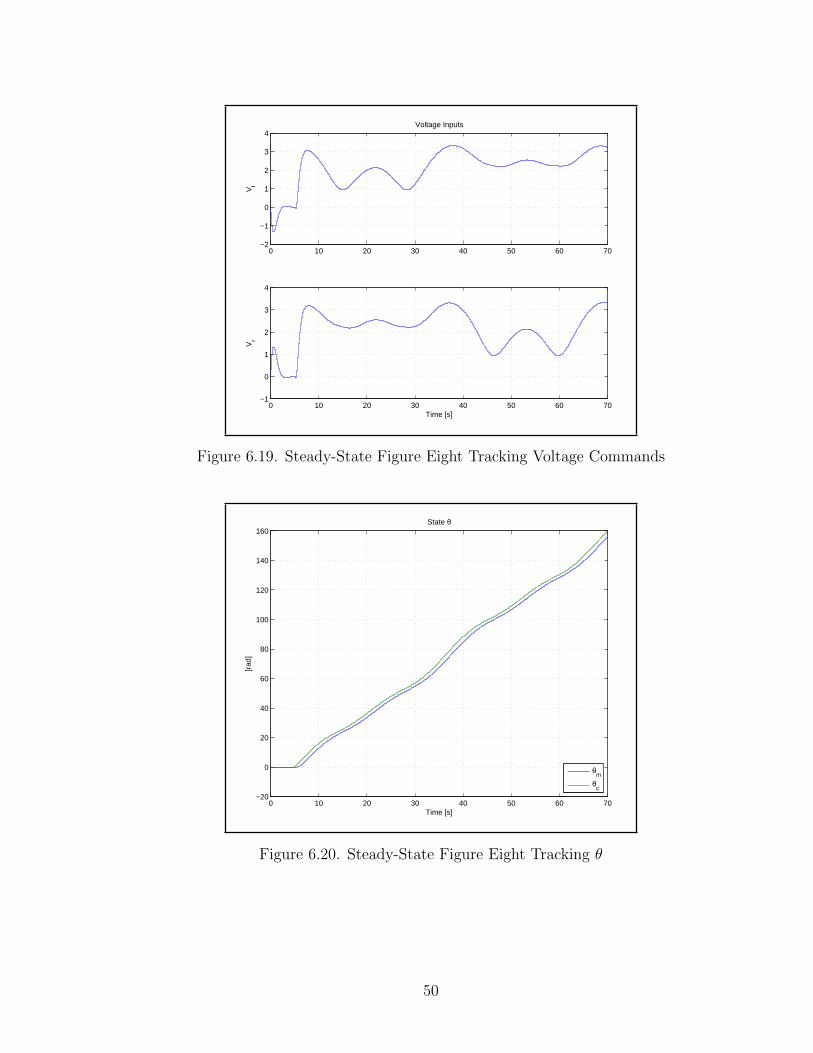
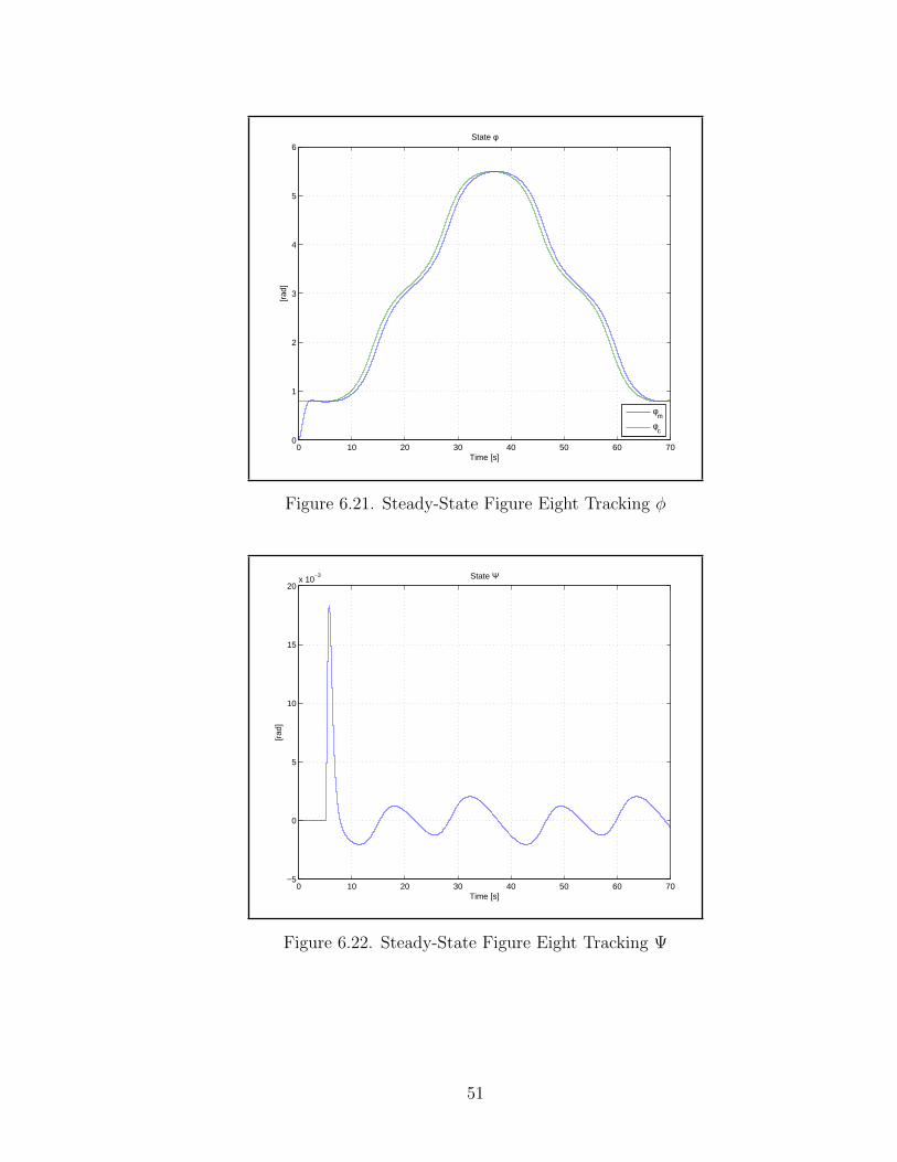
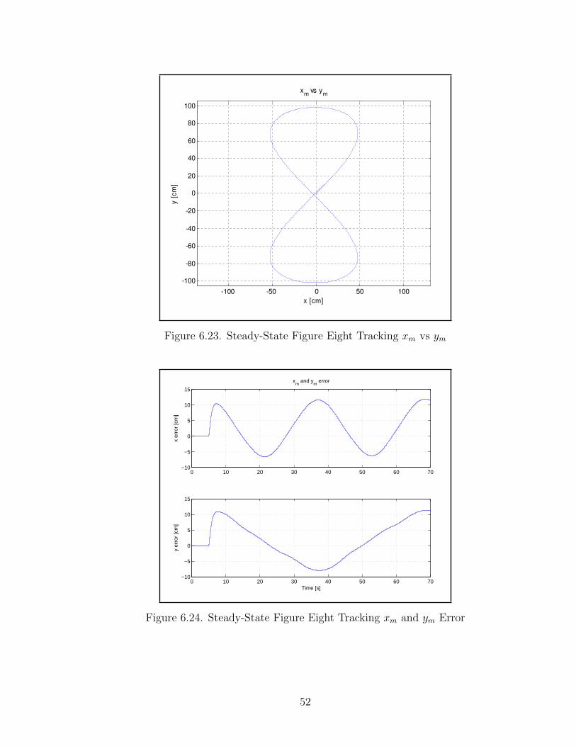
Steady-State Tracking

The following plots show how the system responds to the commands to a

figure eight with the TFBG steady-state design. Figures 6.20 and 6.21 clearly

show that there is a delay in both θ and φ. This delay results in a figure eight that

is shifted as seen in Figure 6.23. The figure eight is clearly out of the limits of ± 50

cm on the x axis and slightly out of ± 100 cm in the y axis. Figure 6.23 shows the

extent of the error in both x and y. The trend seems to show that as time passes

the figure eight would continue to shift to the negative x and y axis. Figure 6.22

shows that the robot will remain balanced while maneuvering the figure eight.

49

0 10 20 30 40 50 60 70−2

−1

0

1

2

3

4

Vl

Voltage Inputs

0 10 20 30 40 50 60 70−1

0

1

2

3

4

Vr

Time [s]

Figure 6.19. Steady-State Figure Eight Tracking Voltage Commands

0 10 20 30 40 50 60 70−20

0

20

40

60

80

100

120

140

160

Time [s]

[rad

]

State θ

θm

θc

Figure 6.20. Steady-State Figure Eight Tracking θ

50

0 10 20 30 40 50 60 700

1

2

3

4

5

6

Time [s]

[rad

]

State φ

φm

φc

Figure 6.21. Steady-State Figure Eight Tracking φ

0 10 20 30 40 50 60 70−5

0

5

10

15

20x 10

−3

Time [s]

[rad

]

State Ψ

Figure 6.22. Steady-State Figure Eight Tracking Ψ

51

-100 -50 0 50 100

-100

-80

-60

-40

-20

0

20

40

60

80

100

x [cm]

y [

cm

]

xm

vs ym

Figure 6.23. Steady-State Figure Eight Tracking xm vs ym

0 10 20 30 40 50 60 70−10

−5

0

5

10

15

x er

ror

[cm

]

xm

and ym

error

0 10 20 30 40 50 60 70−10

−5

0

5

10

15

y er

ror

[cm

]

Time [s]

Figure 6.24. Steady-State Figure Eight Tracking xm and ym Error

52

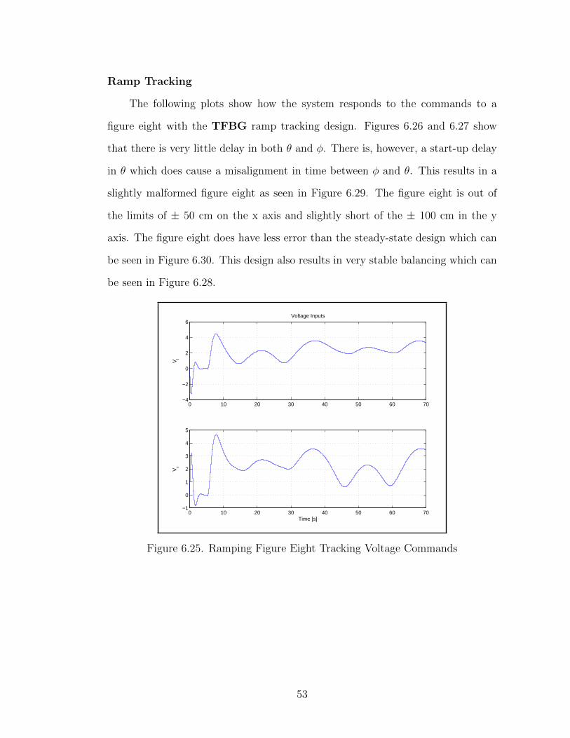
Ramp Tracking

The following plots show how the system responds to the commands to a

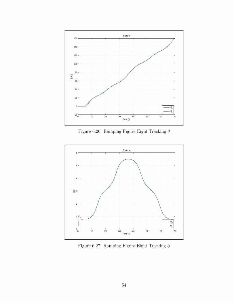
figure eight with the TFBG ramp tracking design. Figures 6.26 and 6.27 show

that there is very little delay in both θ and φ. There is, however, a start-up delay

in θ which does cause a misalignment in time between φ and θ. This results in a

slightly malformed figure eight as seen in Figure 6.29. The figure eight is out of

the limits of ± 50 cm on the x axis and slightly short of the ± 100 cm in the y

axis. The figure eight does have less error than the steady-state design which can

be seen in Figure 6.30. This design also results in very stable balancing which can

be seen in Figure 6.28.

0 10 20 30 40 50 60 70−4

−2

0

2

4

6

Vl

Voltage Inputs

0 10 20 30 40 50 60 70−1

0

1

2

3

4

5

Vr

Time [s]

Figure 6.25. Ramping Figure Eight Tracking Voltage Commands

53

0 10 20 30 40 50 60 70−20

0

20

40

60

80

100

120

140

160

Time [s]

[rad

]

State θ

θm

θc

Figure 6.26. Ramping Figure Eight Tracking θ

0 10 20 30 40 50 60 700

1

2

3

4

5

6

Time [s]

[rad

]

State φ

φm

φc

Figure 6.27. Ramping Figure Eight Tracking φ

54

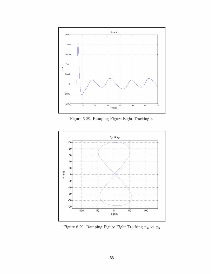
0 10 20 30 40 50 60 70−0.01

−0.005

0

0.005

0.01

0.015

0.02

0.025

Time [s]

[rad

]

State Ψ

Figure 6.28. Ramping Figure Eight Tracking Ψ

-100 -50 0 50 100

-100

-80

-60

-40

-20

0

20

40

60

80

100

x [cm]

y [

cm

]

xm

vs ym

Figure 6.29. Ramping Figure Eight Tracking xm vs ym

55

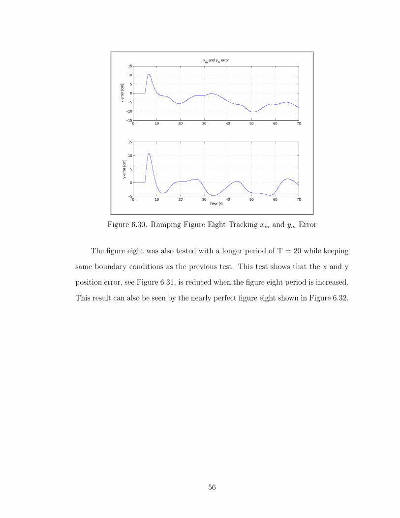
0 10 20 30 40 50 60 70−15

−10

−5

0

5

10

15

x er

ror

[cm

]

xm

and ym

error

0 10 20 30 40 50 60 70−5

0

5

10

15

y er

ror

[cm

]

Time [s]

Figure 6.30. Ramping Figure Eight Tracking xm and ym Error

The figure eight was also tested with a longer period of T = 20 while keeping

same boundary conditions as the previous test. This test shows that the x and y

position error, see Figure 6.31, is reduced when the figure eight period is increased.

This result can also be seen by the nearly perfect figure eight shown in Figure 6.32.

56

0 20 40 60 80 100 120 140−4

−2

0

2

4

6

x er

ror

[cm

]

xm

and ym

error

0 20 40 60 80 100 120 140−2

0

2

4

6

y er

ror

[cm

]

Time [s]

Figure 6.31. Slow Figure Eight Tracking xm and ym Error

-100 -50 0 50 100

-100

-80

-60

-40

-20

0

20

40

60

80

100

x [cm]

y [

cm

]

xm

vs ym

Figure 6.32. Slow Figure Eight Tracking xm vs ym

57

CHAPTER 7

Hardware Testing

The TFBG steady-state tracking design had better performance in simula-

tion and best stability margins. During the hardware experiments the high gains

associated with the TFBG steady-state tracking design made it difficult to im-

plement in hardware. Increasing the settling time for the TFBG steady-state

tracking design may have resulted in a working hardware system; however, this

would have decreased the performance. Therefore, the TFBG ramp tracking de-

sign was implemented in hardware. The controller is implemented in Simulink and

the top level design is shown in Figure 7.1.

58

Motor_r

motor_l

Vbatt

gy ro

theta_m_r

theta_m_l

Input / Output

& calibration / fi ltering

single

Round = Simplest

single

Round = Simplest

data out

Control Enable

theta cmd

phi cmd1

Bluetooth Coms

theta_cmd

phi_cmd

theta_m_l

theta_m_r

gy ro

battery

pwm_l

pwm_r

data

Balance & Drive Control

Figure 7.1. Robot Software

There are three main blocks used in the hardware controller. The sensor inputs

and actuator outputs are found in the “Input/Output & Calibration / Filtering”

block shown in Figure 7.2. The block receives the encoder inputs from each motor

in degrees, the battery voltage in mV, time in ms, and the angular velocity from

the gyro in deg/sec. The battery voltage is filtered with a 10 Hz low pass filter and

59

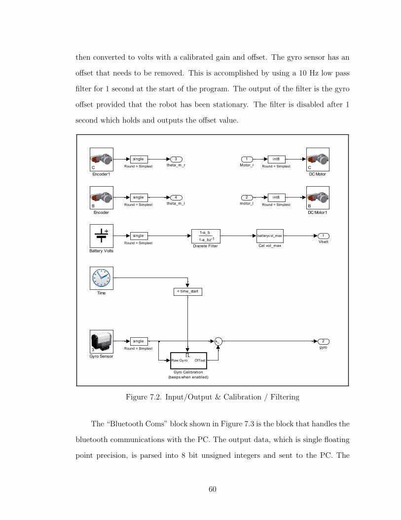
then converted to volts with a calibrated gain and offset. The gyro sensor has an

offset that needs to be removed. This is accomplished by using a 10 Hz low pass

filter for 1 second at the start of the program. The output of the filter is the gyro

offset provided that the robot has been stationary. The filter is disabled after 1

second which holds and outputs the offset value.

4

theta_m_l

3

theta_m_r

2

gyro

1

Vbatt

Time

3

Gyro SensorRaw Gy ro Of f set

Gyro Calibration

(beeps when enabled)

C

Encoder1

B

Encoder

1-a_b

1-a_bz -1

Discrete Filter

single

Round = Simplest

int8

Round = Simplest

single

Round = Simplest

single

Round = Simplest

single

Round = Simplest

int8

Round = Simplest

B

DC Motor1

C

DC Motor

< time_start

batteryv ol_max

Cal vol_max

Battery Volts

2

motor_l

1

Motor_r

Figure 7.2. Input/Output & Calibration / Filtering

The “Bluetooth Coms” block shown in Figure 7.3 is the block that handles the

bluetooth communications with the PC. The output data, which is single floating

point precision, is parsed into 8 bit unsigned integers and sent to the PC. The

60

input data also requires reconstruction from 8 bit unsigned integers from the PC.

The enable signal is converted from an 8 bit unsigned integer to boolean where a

1 enables the tracking system. θ and φ commands are converted from four 8 bit

unsigned integers to 32 bit floats.

3

phi cmd1

2

theta cmd

1

Control Enable

by te3

by te2

by te1

by te0

out

by te3

by te2

by te1

by te0

out

Memory

boolean

Data 1

Data 2

Data 3

Data 4

Data 5

Data 6

Data 7

Data 8

Data 9

Data 10

Data Out

Data Array

Tx

Rx

size

BT Interface

1

data out

Figure 7.3. Bluetooth Coms

The final block “Balance & Drive Control” shown in Figure 7.4 contains the

controller, implemented with three subblocks and is enabled through the bluetooth

communications. The “States” block is shown in Figure 7.5 and is used to calculate

the states from the three sensor inputs. In this block, all sensor inputs are converted

from degrees to radians. The “Drift Comp” contains a 0.04 Hz low pass filter of

the gyro signal to remove any DC offset that may accumulate in the gyro. The

equations used in the “States” block are discussed in Section 5.4. The “Balance

& Drive Control” block also contains the PWM generations shown in Figure 7.6.

This block contains the limiters and the equations for the outputs as specified in

Section 5.4.

61

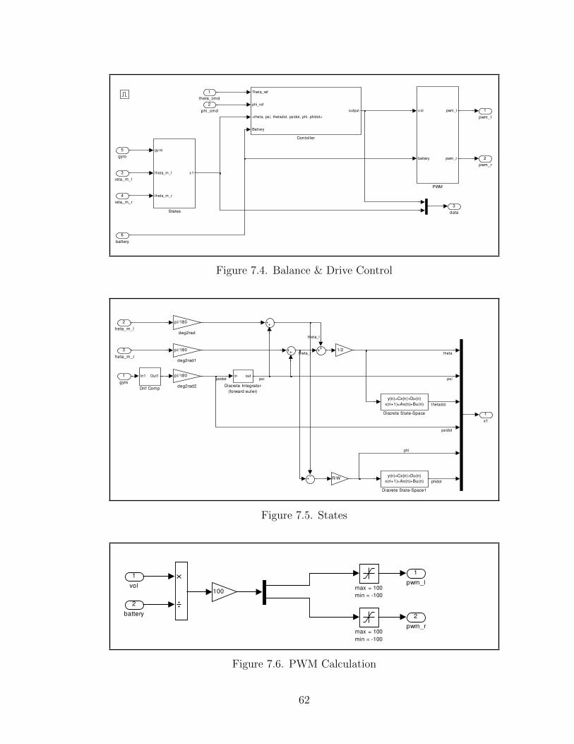
3

data

2

pwm_r

1

pwm_l

gy ro

theta_m_l

theta_m_r

x1

States

v ol

battery

pwm_l

pwm_r

PWM

Theta_ref

phi_ref

<theta, psi, thetadot, psidot, phi, phidot>

Battery

output

Contoller

6

battery

5

gyro

4

theta_m_r

3

theta_m_l

2

phi_cmd

1

theta_cmd

Figure 7.4. Balance & Drive Control

1

x1

pi/180

deg2rad2

pi/180

deg2rad1

pi/180

deg2rad

R/W

1/2

In1 Out1

Dri f Comp

y(n)=Cx(n)+Du(n)

x(n+1)=Ax(n)+Bu(n)

Discrete State-Space1

y(n)=Cx(n)+Du(n)

x(n+1)=Ax(n)+Bu(n)

Discrete State-Space

in out

Discrete Integrator

(forward euler)

3

theta_m_r

2

theta_m_l

1

gyro

theta

psidot

psidot

theta_r

theta_l

thetadot

psipsi

phidot

phi

Figure 7.5. States

2

pwm_r

1

pwm_l

max = 100

min = -100

max = 100

min = -100100

2

battery

1

vol

Figure 7.6. PWM Calculation

62

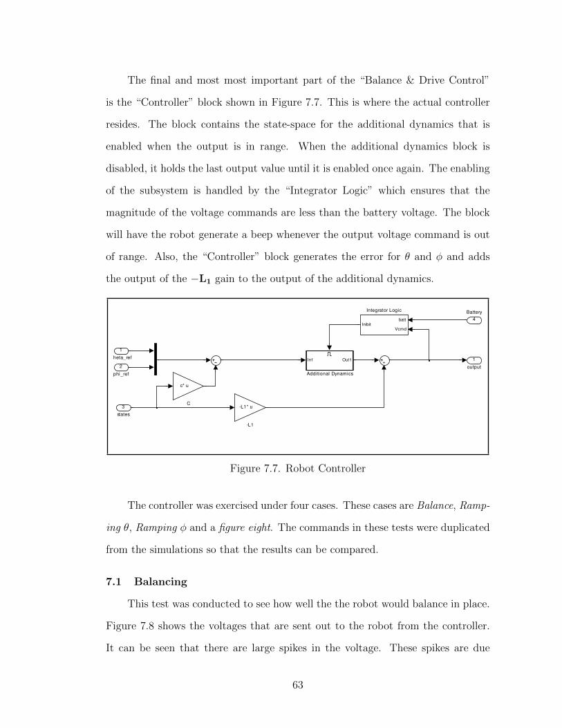
The final and most most important part of the “Balance & Drive Control”

is the “Controller” block shown in Figure 7.7. This is where the actual controller

resides. The block contains the state-space for the additional dynamics that is

enabled when the output is in range. When the additional dynamics block is

disabled, it holds the last output value until it is enabled once again. The enabling

of the subsystem is handled by the “Integrator Logic” which ensures that the

magnitude of the voltage commands are less than the battery voltage. The block

will have the robot generate a beep whenever the output voltage command is out

of range. Also, the “Controller” block generates the error for θ and φ and adds

the output of the −L1 gain to the output of the additional dynamics.

1

output

batt

VcmdInibit

Integrator Logic

c* u

C

In1 Out1

Addi tional Dynamics

-L1* u

-L1

4

Battery

3

states

2

phi_ref

1

Theta_ref

Figure 7.7. Robot Controller

The controller was exercised under four cases. These cases are Balance, Ramp-

ing θ, Ramping φ and a figure eight. The commands in these tests were duplicated

from the simulations so that the results can be compared.

7.1 Balancing

This test was conducted to see how well the the robot would balance in place.

Figure 7.8 shows the voltages that are sent out to the robot from the controller.

It can be seen that there are large spikes in the voltage. These spikes are due

63

to the system trying to respond to the non-linear dead-band that is introduced

by friction and mechanical slop in the motor gears. This is also compounded by

the low resolution of the sensors. These effects are what dictated using a slower

settling time for the controller. This also made it difficult to place an observer as

part of the controller because of the large voltage spikes that would be fed into a

linear observer. The states and their responses are shown in Figures 7.9 - 7.14.

0 2 4 6 8 10 12 14 16 18 20−10

−5

0

5

10

Vl

Voltage Inputs

0 2 4 6 8 10 12 14 16 18 20−10

−5

0

5

10

Vr

Time [s]

Figure 7.8. Balancing Voltage Commands

64

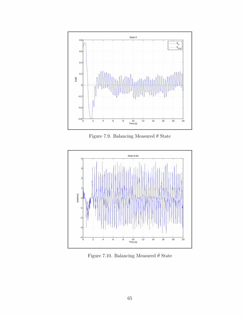
0 2 4 6 8 10 12 14 16 18 20−0.6

−0.4

−0.2

0

0.2

0.4

0.6

0.8

Time [s]

[rad

]

State θ

θ

m

θcmd

Figure 7.9. Balancing Measured θ State

0 2 4 6 8 10 12 14 16 18 20−4

−3

−2

−1

0

1

2

3

4

Time [s]

[rad

/sec

]

State θ dot

Figure 7.10. Balancing Measured θ State

65

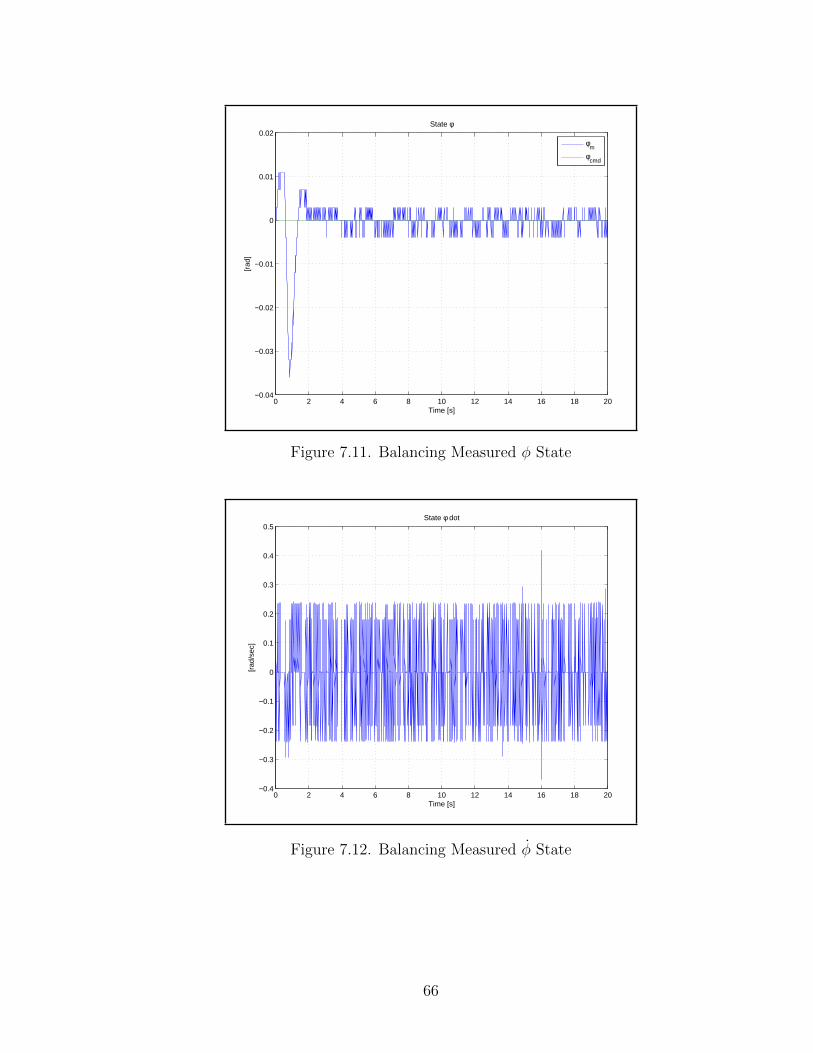
0 2 4 6 8 10 12 14 16 18 20−0.04

−0.03

−0.02

−0.01

0

0.01

0.02

Time [s]

[rad

]

State φ

φ

m

φcmd

Figure 7.11. Balancing Measured φ State

0 2 4 6 8 10 12 14 16 18 20−0.4

−0.3

−0.2

−0.1

0

0.1

0.2

0.3

0.4

0.5

Time [s]

[rad

/sec

]

State φ dot

Figure 7.12. Balancing Measured φ State

66

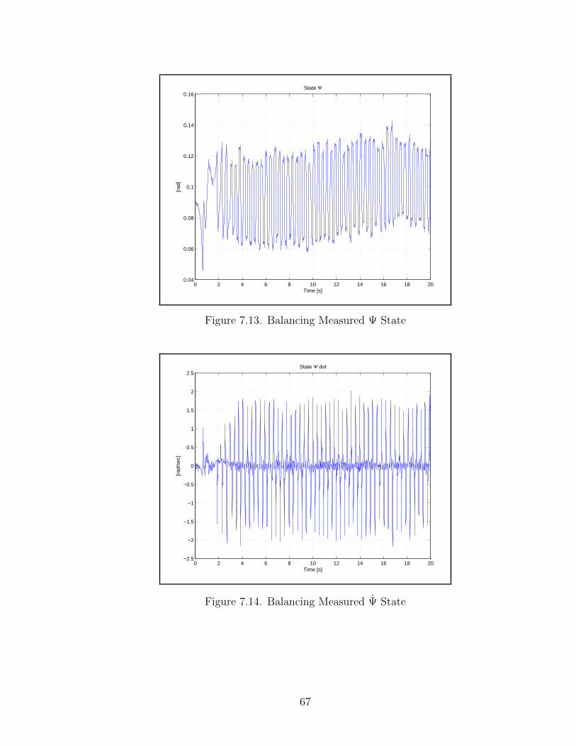
0 2 4 6 8 10 12 14 16 18 200.04

0.06

0.08

0.1

0.12

0.14

0.16

Time [s]

[rad

]

State Ψ

Figure 7.13. Balancing Measured Ψ State

0 2 4 6 8 10 12 14 16 18 20−2.5

−2

−1.5

−1

−0.5

0

0.5

1

1.5

2

2.5

Time [s]

[rad

/sec

]

State Ψ dot

Figure 7.14. Balancing Measured Ψ State

67

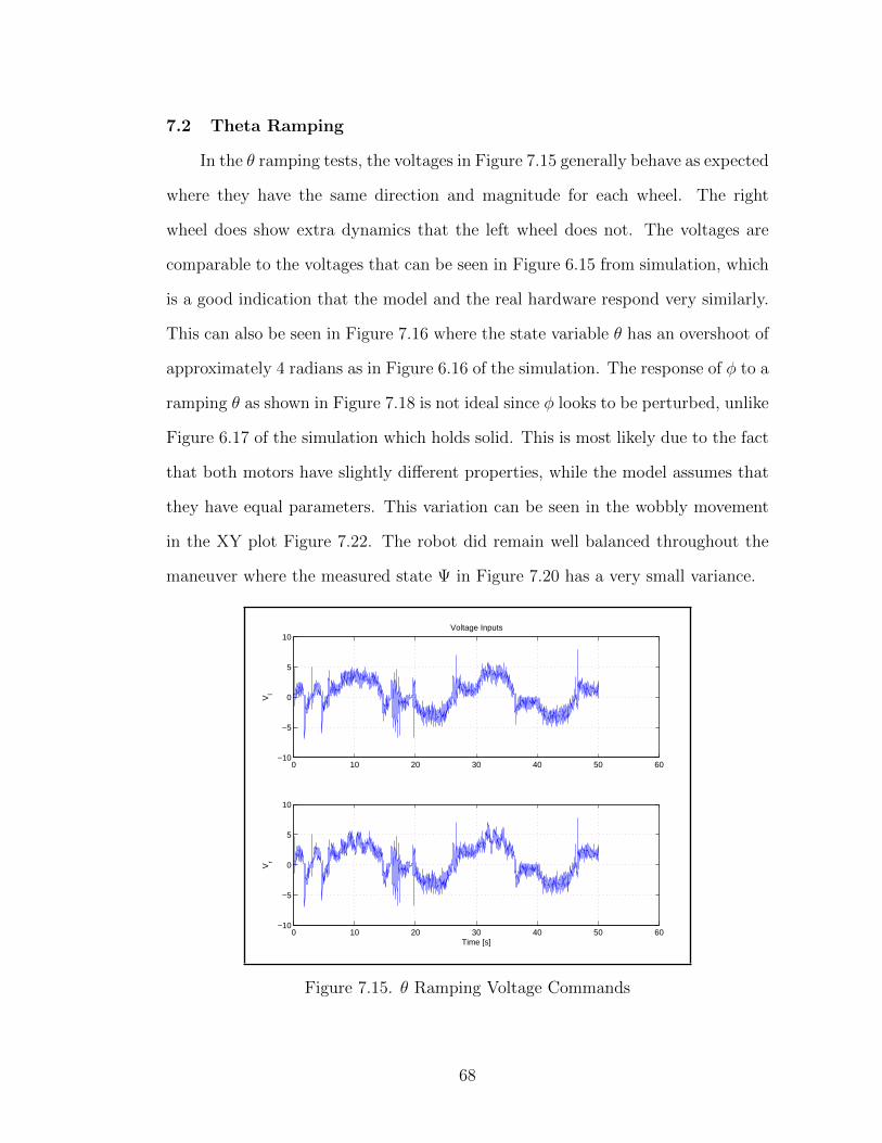
7.2 Theta Ramping

In the θ ramping tests, the voltages in Figure 7.15 generally behave as expected

where they have the same direction and magnitude for each wheel. The right

wheel does show extra dynamics that the left wheel does not. The voltages are

comparable to the voltages that can be seen in Figure 6.15 from simulation, which

is a good indication that the model and the real hardware respond very similarly.

This can also be seen in Figure 7.16 where the state variable θ has an overshoot of

approximately 4 radians as in Figure 6.16 of the simulation. The response of φ to a

ramping θ as shown in Figure 7.18 is not ideal since φ looks to be perturbed, unlike

Figure 6.17 of the simulation which holds solid. This is most likely due to the fact

that both motors have slightly different properties, while the model assumes that

they have equal parameters. This variation can be seen in the wobbly movement

in the XY plot Figure 7.22. The robot did remain well balanced throughout the

maneuver where the measured state Ψ in Figure 7.20 has a very small variance.

0 10 20 30 40 50 60−10

−5

0

5

10

Vl

Voltage Inputs

0 10 20 30 40 50 60−10

−5

0

5

10

Vr

Time [s]

Figure 7.15. θ Ramping Voltage Commands

68

0 10 20 30 40 50 60−5

0

5

10

15

20

25

Time [s]

[rad

]

State θ

θ

m

θcmd

Figure 7.16. θ Ramping Measured θ State

0 10 20 30 40 50 60−6

−4

−2

0

2

4

6

Time [s]

[rad

/sec

]

State θ dot

Figure 7.17. θ Ramping Measured θ State

69

0 10 20 30 40 50 60−0.08

−0.06

−0.04

−0.02

0

0.02

0.04

0.06

0.08

Time [s]

[rad

]

State φ

φ

m

φcmd

Figure 7.18. θ Ramping Measured φ State

0 10 20 30 40 50 60−0.8

−0.6

−0.4

−0.2

0

0.2

0.4

0.6

Time [s]

[rad

/sec

]

State φ dot

Figure 7.19. θ Ramping Measured φ State

70

0 10 20 30 40 50 60−0.08

−0.06

−0.04

−0.02

0

0.02

0.04

0.06

Time [s]

[rad

]

State Ψ

Figure 7.20. θ Ramping Measured Ψ State

0 10 20 30 40 50 60−2

−1.5

−1

−0.5

0

0.5

1

1.5

2

2.5

Time [s]

[rad

/sec

]

State Ψ dot

Figure 7.21. θ Ramping Measured Ψ State

71

−20 0 20 40 60 80 100−1.4

−1.2

−1

−0.8

−0.6

−0.4

−0.2

0

x [cm]

y [c

m]

xm

vs ym

Figure 7.22. θ Ramping XY Plot

7.3 Phi Ramping

In the φ ramping tests, the voltages in Figure 7.23 are comparable to the

voltages that can be seen in Figure 6.11. The voltages are opposite in direction

and have equal magnitude for each wheel. Figure 7.25 has an overshoot of ap-

proximately 0.5 radians as in Figure 6.13 of the simulation. The response of θ

to a ramping φ as shown in Figure 7.26 is not ideal since θ is perturbed, unlike

Figure 6.12 of the simulation which holds solid. This variation can be seen in the

wobbly movement in the XY plot Figure 7.30. The robot remained well balanced

throughout the maneuver as shown in the measured state Ψ in Figure 7.28 .

72

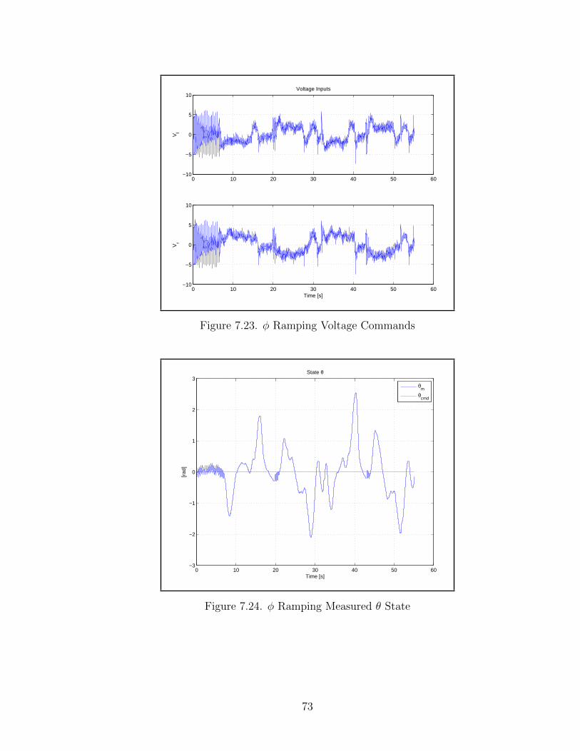
0 10 20 30 40 50 60−10

−5

0

5

10

Vl

Voltage Inputs

0 10 20 30 40 50 60−10

−5

0

5

10

Vr

Time [s]

Figure 7.23. φ Ramping Voltage Commands

0 10 20 30 40 50 60−3

−2

−1

0

1

2

3

Time [s]

[rad

]

State θ

θ

m

θcmd

Figure 7.24. φ Ramping Measured θ State

73

0 10 20 30 40 50 60−4

−3

−2

−1

0

1

2

3

4

Time [s]

[rad

/sec

]

State θ dot

Figure 7.25. φ Ramping Measured θ State

0 10 20 30 40 50 60−1

0

1

2

3

4

5

6

7

Time [s]

[rad

]

State φ

φ

m

φcmd

Figure 7.26. φ Ramping Measured φ State

74

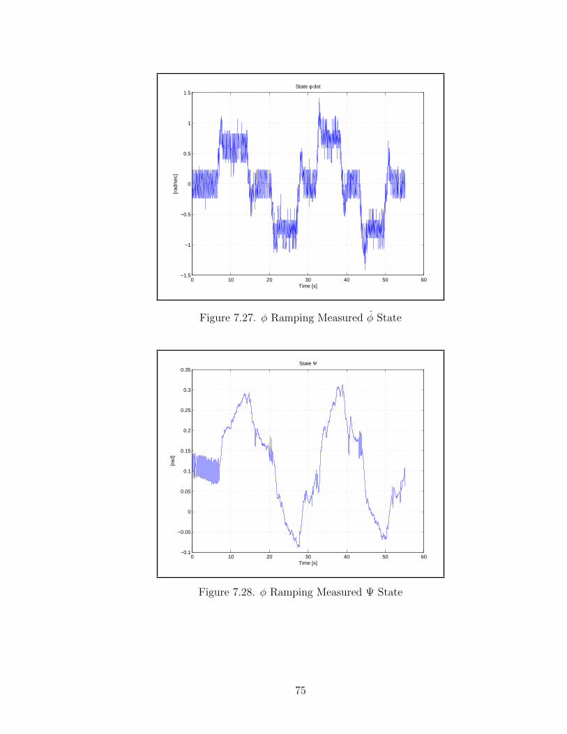
0 10 20 30 40 50 60−1.5

−1

−0.5

0

0.5

1

1.5

Time [s]

[rad

/sec

]

State φ dot

Figure 7.27. φ Ramping Measured φ State

0 10 20 30 40 50 60−0.1

−0.05

0

0.05

0.1

0.15

0.2

0.25

0.3

0.35

Time [s]

[rad

]

State Ψ

Figure 7.28. φ Ramping Measured Ψ State

75

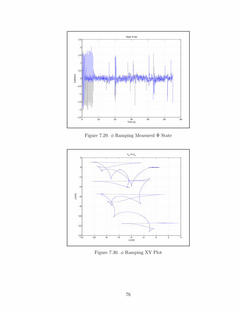
0 10 20 30 40 50 60−2.5

−2

−1.5

−1

−0.5

0

0.5

1

1.5

2

2.5

Time [s]

[rad

/sec

]

State Ψ dot

Figure 7.29. φ Ramping Measured Ψ State

−12 −10 −8 −6 −4 −2 0 2 4−14

−12

−10

−8

−6

−4

−2

0

2

x [cm]

y [c

m]

xm

vs ym

Figure 7.30. φ Ramping XY Plot

76

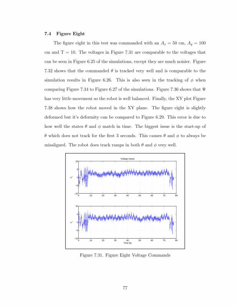
7.4 Figure Eight

The figure eight in this test was commanded with an Ax = 50 cm, Ay = 100

cm and T = 10. The voltages in Figure 7.31 are comparable to the voltages that

can be seen in Figure 6.25 of the simulations, except they are much noisier. Figure

7.32 shows that the commanded θ is tracked very well and is comparable to the

simulation results in Figure 6.26. This is also seen in the tracking of φ when

comparing Figure 7.34 to Figure 6.27 of the simulations. Figure 7.36 shows that Ψ

has very little movement so the robot is well balanced. Finally, the XY plot Figure

7.38 shows how the robot moved in the XY plane. The figure eight is slightly

deformed but it’s deformity can be compared to Figure 6.29. This error is due to

how well the states θ and φ match in time. The biggest issue is the start-up of

θ which does not track for the first 3 seconds. This causes θ and φ to always be

misaligned. The robot does track ramps in both θ and φ very well.

0 10 20 30 40 50 60 70 80−10

−5

0

5

10

Vl

Voltage Inputs

0 10 20 30 40 50 60 70 80−10

−5

0

5

10

Vr

Time [s]

Figure 7.31. Figure Eight Voltage Commands

77

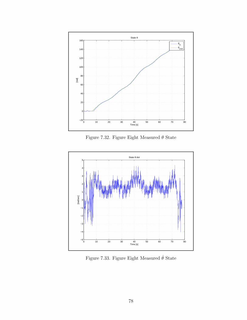
0 10 20 30 40 50 60 70 80−20

0

20

40

60

80

100

120

140

160

Time [s]

[rad

]

State θ

θ

m

θcmd

Figure 7.32. Figure Eight Measured θ State

0 10 20 30 40 50 60 70 80−5

−4

−3

−2

−1

0

1

2

3

4

5

Time [s]

[rad

/sec

]

State θ dot

Figure 7.33. Figure Eight Measured θ State

78

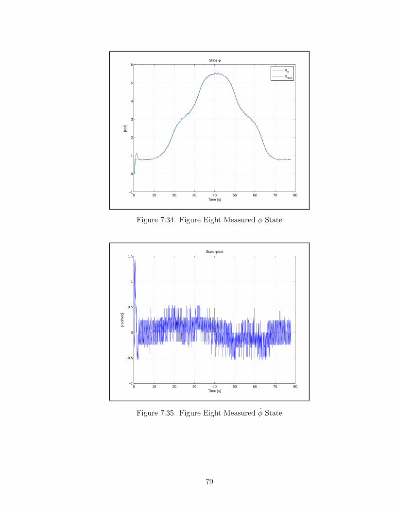
0 10 20 30 40 50 60 70 80−1

0

1

2

3

4

5

6

Time [s]

[rad

]

State φ

φ

m

φcmd

Figure 7.34. Figure Eight Measured φ State

0 10 20 30 40 50 60 70 80−1

−0.5

0

0.5

1

1.5

Time [s]

[rad

/sec

]

State φ dot

Figure 7.35. Figure Eight Measured φ State

79

0 10 20 30 40 50 60 70 80−0.36

−0.34

−0.32

−0.3

−0.28

−0.26

−0.24

−0.22

−0.2

−0.18

−0.16

Time [s]

[rad

]

State Ψ

Figure 7.36. Figure Eight Measured Ψ State

0 10 20 30 40 50 60 70 80−2

−1.5

−1

−0.5

0

0.5

1

1.5

2

Time [s]

[rad

/sec

]

State Ψ dot

Figure 7.37. Figure Eight Measured Ψ State

80

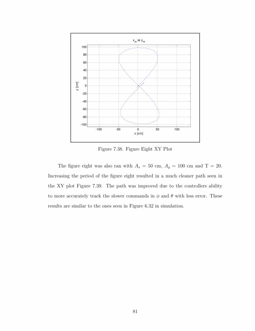
-100 -50 0 50 100

-100

-80

-60

-40

-20

0

20

40

60

80

100

x [cm]

y [

cm

]

xm

vs ym

Figure 7.38. Figure Eight XY Plot

The figure eight was also ran with Ax = 50 cm, Ay = 100 cm and T = 20.

Increasing the period of the figure eight resulted in a much cleaner path seen in

the XY plot Figure 7.39. The path was improved due to the controllers ability

to more accurately track the slower commands in φ and θ with less error. These

results are similar to the ones seen in Figure 6.32 in simulation.

81

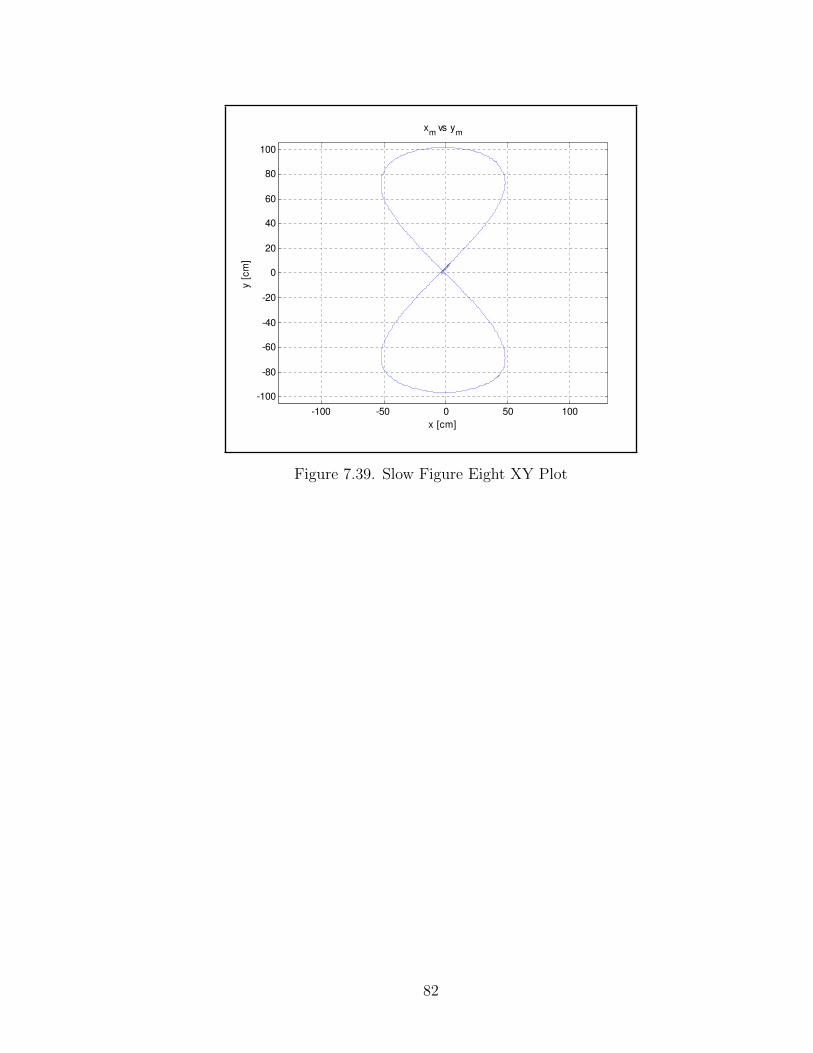
-100 -50 0 50 100

-100

-80

-60

-40

-20

0

20

40

60

80

100

x [cm]

y [

cm

]

xm

vs ym

Figure 7.39. Slow Figure Eight XY Plot

82

CHAPTER 8

Conclusions

The robot is a MIMO system with two inputs and six state variables. In this

thesis the state variables θ and φ are the tracked outputs and all state variables

were regulated. The design of the controller was based on pole placement. The

placement of the poles determined the settling time of the system. Due to non-

linearities in the motors and quantization in the system, the settling time needed

to be increased, which reduced the performance of the controller.

The design of the tracking system placed consideration on hardware con-

straints. Some of these constraints were voltage saturation, quantization and the

dead band in the motors. These effects were predominant while balancing in place.

Quantization introduced a derivative action at low speeds which, if the gains were

too high, would cause the system to be driven into saturation. Decreasing the

settling time also introduced problems with dead band. The dead band forced the

integrators to wind up and again, if the gains were too high, the output would

saturate. To compensate for these non-ideal conditions the settling time was in-

creased. The performance of the digital tracking system as seen in the hardware

and simulation testing was reduced with a higher settling time. The result was

that the state variable θ had a high level of overshoot and the figure eight was

malformed. It was shown that a figure eight with a longer period could be better

tracked. Although it was not shown in this thesis, decreasing the settling time

would result in perfect θ and φ ramp tracking with very little overshoot in sim-

ulations. However, decreasing the settling time does not produce zero error to

tracking xm and ym. Although the error is reduced, the figure eight may still drift

due to start up delay in θ.

83

This thesis provides a basis for future design for a more accurate two-wheeled

robot trajectory tracking. The current design can accurately move back and forth,

and turn under closed-loop control. This would allow movement through a maze

that contains straight paths with turns at the end of the paths. The controller

would have problems with paths that have arcs. These issues are due to the non-

linear kinematic characteristics and non-holonomic constraints of a wheeled mobile

robot [1]. The controller introduced in this thesis relies on θ and φ having zero error

at every instant in time to track complex paths such as a figure eight. When state

variables θ and φ are not synchronized in time the two-wheeled robot will go slightly

off course. One source of this error it that the closed-loop system may have different

delays for θ and φ. Future designs may incorporate an inverse kinematic transform

to compensate for these system dynamics. The inverse kinematic transform would

have the desired trajectory as inputs and produce θ and φ commands that are

compensated for by the system dynamics. Another source of error are disturbances

in the state variable Ψ that results in a disturbance in θ and φ in order to balance.

This could be remedied by having another slower outer-loop controller that corrects

for error in xm and ym.

The feedback control algorithms place, fbg and TFBG were all examined.

Analysis and simulations showed that even though a feedback matrix may have

better stability margins, it may not have the best performance. These algorithms

were all compared to one another in both steady-state tracking and in ramp track-

ing. The place algorithm did not produce very good results, which has been the

case in other studies [2]. TFBG showed the best results. The algorithm searches

for the best stability margins for both inputs. It also searches for a desired sym-

metry in the feedback matrix.

The controller was able to track θ and φ, which was demonstrated in both

84

simulation and in the hardware. The hardware and simulation showed difficulty

in tracking a figure eight at high a high speed. In both simulation and hardware,

slowing down the commands by changing the parameter T from 10 to 20 allowed

the system to track much better. The result was a very slow moving system that

tracked.

List of References

[1] M. Nilulescu, “Controlling a mobile robot along planned trajectories,” CEAI,vol. 7, no. 20, pp. 18–24, 2005.

[2] S. Nawawi, M. Ahmad, J. Osman, A. Husain, and M. Abdollah, “Controllerdesign for two-wheels inverted pendulum mobile robot using PISMC,” 4th Stu-dent Conference on Research and Development, pp. 194 – 199, June 2006.

85

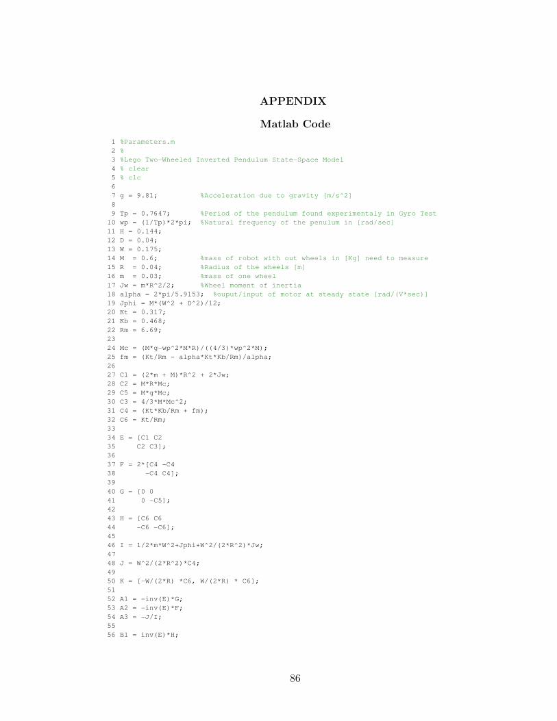
APPENDIX

Matlab Code

1 %Parameters.m

2 %

3 %Lego Two-Wheeled Inverted Pendulum State-Space Model

4 % clear

5 % clc

6

7 g = 9.81; %Acceleration due to gravity [m/s^2]

8

9 Tp = 0.7647; %Period of the pendulum found experimentaly in Gyro Test

10 wp = (1/Tp)*2*pi; %Natural frequency of the penulum in [rad/sec]

11 H = 0.144;

12 D = 0.04;

13 W = 0.175;

14 M = 0.6; %mass of robot with out wheels in [Kg] need to measure

15 R = 0.04; %Radius of the wheels [m]

16 m = 0.03; %mass of one wheel

17 Jw = m*R^2/2; %Wheel moment of inertia

18 alpha = 2*pi/5.9153; %ouput/input of motor at steady state [rad/(V*sec)]

19 Jphi = M*(W^2 + D^2)/12;

20 Kt = 0.317;

21 Kb = 0.468;

22 Rm = 6.69;

23

24 Mc = (M*g-wp^2*M*R)/((4/3)*wp^2*M);

25 fm = (Kt/Rm - alpha*Kt*Kb/Rm)/alpha;

26

27 C1 = (2*m + M)*R^2 + 2*Jw;

28 C2 = M*R*Mc;

29 C5 = M*g*Mc;

30 C3 = 4/3*M*Mc^2;

31 C4 = (Kt*Kb/Rm + fm);

32 C6 = Kt/Rm;

33

34 E = [C1 C2

35 C2 C3];

36

37 F = 2*[C4 -C4

38 -C4 C4];

39

40 G = [0 0

41 0 -C5];

42

43 H = [C6 C6

44 -C6 -C6];

45

46 I = 1/2*m*W^2+Jphi+W^2/(2*R^2)*Jw;

47

48 J = W^2/(2*R^2)*C4;

49

50 K = [-W/(2*R) *C6, W/(2*R) * C6];

51

52 A1 = -inv(E)*G;

53 A2 = -inv(E)*F;

54 A3 = -J/I;

55

56 B1 = inv(E)*H;

86

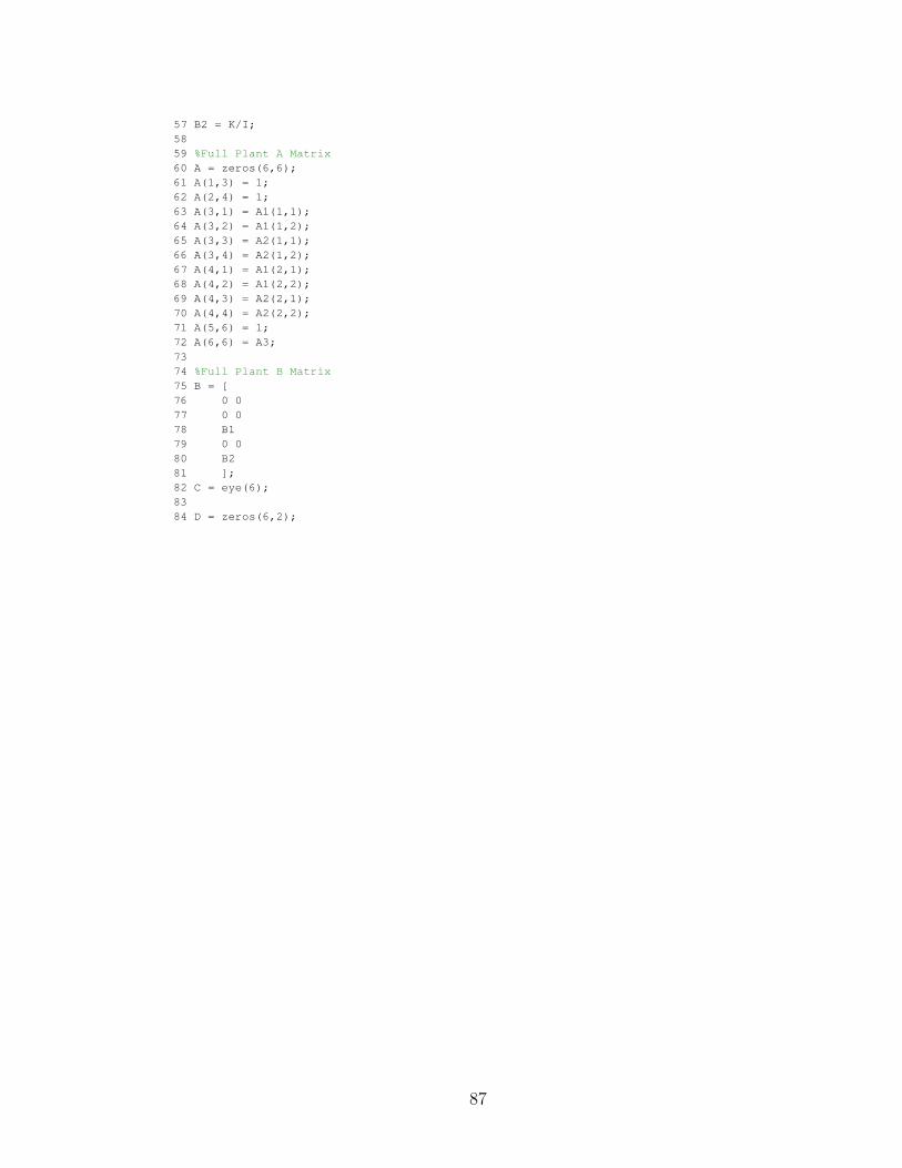
57 B2 = K/I;

58

59 %Full Plant A Matrix

60 A = zeros(6,6);

61 A(1,3) = 1;

62 A(2,4) = 1;

63 A(3,1) = A1(1,1);

64 A(3,2) = A1(1,2);

65 A(3,3) = A2(1,1);

66 A(3,4) = A2(1,2);

67 A(4,1) = A1(2,1);

68 A(4,2) = A1(2,2);

69 A(4,3) = A2(2,1);

70 A(4,4) = A2(2,2);

71 A(5,6) = 1;

72 A(6,6) = A3;

73

74 %Full Plant B Matrix

75 B = [

76 0 0

77 0 0

78 B1

79 0 0

80 B2

81 ];

82 C = eye(6);

83

84 D = zeros(6,2);

87

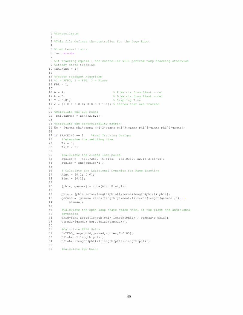
1 %Controller.m

2

3 %This file defines the controller for the Lego Robot

4

5 %load bessel roots

6 load sroots

7

8 %If Tracking equals 1 the controller will perfrom ramp tracking otherwise

9 %steady-state tracking

10 TRACKING = 1;

11

12 %Vector Feedback Algorithm

13 %1 = RFBG, 2 = FBG, 3 = Place

14 FBA = 1;

15

16 A = A; % A Matrix from Plant model

17 b = B; % B Matrix from Plant model

18 T = 0.01; % Sampling Time

19 c = [1 0 0 0 0 0; 0 0 0 0 1 0]; % States that are tracked

20

21 %Calculate the ZOH model

22 [phi,gamma] = zohe(A,b,T);

23

24 %Calculate the controllabilty matrix

25 Wc = [gamma phi*gamma phi^2*gamma phi^3*gamma phi^4*gamma phi^5*gamma];

26

27 if TRACKING == 1 %Ramp Tracking Designs

28 %Determine the settling time

29 Ts = 3;

30 Ts_2 = 5;

31

32 %Calculate the closed loop poles

33 spoles = [-460.7253, -6.6185, -182.0352, s2/Ts_2,s5/Ts];

34 zpoles = exp(spoles*T);

35

36 % Calculate the Additional Dynamics for Ramp Tracking

37 Aint = [0 1; 0 0];

38 Bint = [0;1];

39

40 [phia, gammaa] = zohe(Aint,Bint,T);

41

42 phia = [phia zeros(length(phia));zeros(length(phia)) phia];

43 gammaa = [gammaa zeros(length(gammaa),1);zeros(length(gammaa),1)...

44 gammaa];

45

46 %Calculate the open loop state-space Model of the plant and additional

47 %dynamics

48 phid=[phi zeros(length(phi),length(phia)); gammaa*c phia];

49 gammad=[gamma; zeros(size(gammaa))];

50

51 %Calculate TFBG Gains

52 L=TFBG_ramp(phid,gammad,zpoles,T,0.05);

53 L11=L(:,1:length(phi));

54 L21=L(:,length(phi)+1:length(phia)+length(phi));

55

56 %Calculate FBG Gains

88

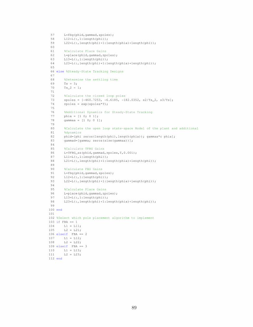
57 L=fbg(phid,gammad,zpoles);



60

61 %Calculate Place Gains

62 L=place(phid,gammad,zpoles);



65

66 else %Steady-State Tracking Designs

67

68 %Determine the settling time

69 Ts = 3;

70 Ts_2 = 1;

71

72 %Calculate the closed loop poles

73 spoles = [-460.7253, -6.6185, -182.0352, s2/Ts_2, s3/Ts];

74 zpoles = exp(spoles*T);

75

76 %Additional Dynamics for Steady-State Tracking

77 phia = [1 0; 0 1];

78 gammaa = [1 0; 0 1];

79

80 %Calculate the open loop state-space Model of the plant and additional

81 %dynamics

82 phid=[phi zeros(length(phi),length(phia)); gammaa*c phia];

83 gammad=[gamma; zeros(size(gammaa))];

84

85 %Calculate TFBG Gains

86 L=TFBG_ss(phid,gammad,zpoles,T,0.001);



89

90 %Calculate FBG Gains

91 L=fbg(phid,gammad,zpoles);



94

95 %Calculate Place Gains

96 L=place(phid,gammad,zpoles);



99

100 end

101

102 %Select which pole placement algorithm to implement

103 if FBA == 1

104 L1 = L11;

105 L2 = L21;

106 elseif FBA == 2

107 L1 = L12;

108 L2 = L22;

109 elseif FBA == 3

110 L1 = L13;

111 L2 = L23;

112 end

89

113

114

115 %filtered derivative

116 ts_f = 0.025;

117 b = poly(s2/ts_f);

118 fil1 = tf([b(3) 0],b);

119 [fil1n fil1d] = tfdata(c2d(fil1,T));

120

121 Af = [0 1; -b(3)/b(1) -b(2)/b(1)];

122 Bf = [0; b(3)/b(1)];

123 Cf = [0 1];

124 Df = 0;

125

126 [phif gammaf] = zohe(Af,Bf,T);

127

128 %Addtional Dynamics Hold Parameter

129 int_inhibit_Bat = 0.95;

130

131 % Task Sample Rates

132 ts1 = T; % ts1 sample time [sec] main control

133 ts3 = 0.1; % ts3 sample time [sec] battery voltage

134

135 time_start = 1000; % gyro calibration time

136

137 % Low Pass Filter Coefficients

138 a_b = exp(-10*(2*pi)*ts1); % average battery value

139 a_gc = exp(-10*(2*pi)*ts1); % initial calibrate gyro offset

140 a_gd = exp(-0.04*(2*pi)*ts1); % Drifting gyro offset;

141

142 % User Setting Values

143 sound_freq = 440; % sound frequency [Hz]

144

145

146 %% Analyis Calculate Stability Margins

147

148 %TFBG

149 L1m = [L11, L21];

150 RFBDDelta = msm(phid,gammad,L1m,T);

151 RFBDUGM = 20*log10(1+RFBDDelta);

152 RFBDLGM = 20*log10(1-RFBDDelta);

153 RFBDPM = 2*180/pi*asin(RFBDDelta/2);

154

155 %FBG

156 L2m = [L12, L22];

157 FBDDelta = msm(phid,gammad,L2m,T);

158 FBDUGM = 20*log10(1+FBDDelta);

159 FBDLGM = 20*log10(1-FBDDelta);

160 FBDPM = 2*180/pi*asin(FBDDelta/2);

161

162 %Place

163 L3m = [L13, L23];

164 PlaceDelta = msm(phid,gammad,L3m,T);

165 PlaceUGM = 20*log10(1+PlaceDelta);

166 PlaceLGM = 20*log10(1-PlaceDelta);

167 PlacePM = 2*180/pi*asin(PlaceDelta/2);

90

BIBLIOGRAPHY

Burl, J. B., Linear Optimal Control. Reading, Massachusetts, United States ofAmerica: Addison-Wesley, 1998.

Chikamasa, T., “Nxt gamepad,” January 2009, unpublished. [Online]. Available:http://lejos-osek.sourceforge.net/nxtgamepad.htm

Chikamasa, T., “Embedded coder robot nxt modeling tips,” April2010, unpublished. [Online]. Available: http://www.mathworks.com/matlabcentral/fileexchange/13399-embedded-coder-robot-nxt-demo?controller=file infos&download=true

Jones, J. P., McArthur, C., and Young, T., VU-LEGO Real Time Target: User’sGuide, 1st ed., Center for Nonlinear Dynamics and Control, Villanova Uni-versity, Villanova PA 19085, United States of America, February 2011.

Jung, S. and Kim, S. S., “Control experiment of a wheel-driven mobile invertedpendulum using neural network,” IEEE Transactions On Control SystemsTechnology, vol. 16, pp. 297–303, March 2008.

Kautsky, J., Nichols, N., and Dooren, P. V., “Robust pole assignment in linear statefeedback,” International Journal of Control, vol. 41, pp. 1129–1155, 1985.

Loan, C. F. V., “Computing integrals involving the matrix exponential,” IEEETransactions on Automatic Control, vol. AC-23, pp. 395–404, June 1978.

Nawawi, S., Ahmad, M., Osman, J., Husain, A., and Abdollah, M., “Controllerdesign for two-wheels inverted pendulum mobile robot using PISMC,” 4thStudent Conference on Research and Development, pp. 194 – 199, June 2006.

Nilulescu, M., “Controlling a mobile robot along planned trajectories,” CEAI,vol. 7, no. 20, pp. 18–24, 2005.

Sima, V., Tits, A. L., and Yang, Y., “Computational experience with robust poleassignment algorithms,” Conference on Computer Aided Control Systems De-sign, vol. WeA01.6, pp. 36–41, October 2006.

Vaccaro, R. J., Digital Control A State-Space Approch. New York, New York,United States of America: McGraw-Hill, Inc, 1995.

Vaccaro, R. J., Department of Electrical, Computer, and Biomedical Engineering,University of Rhode Island, Kingston RI 02881, United States of America,October 2011, personal communication.

91

http://lejos-osek.sourceforge.net/nxtgamepad.htm




Yamamoto, Y., “Nxtway-gs model-based design - control of self-balancing two-wheeled robot built with lego mindstorms nxt -,” May 2009, unpublished. [On-line]. Available: http://www.mathworks.com/matlabcentral/fileexchange/19147-nxtway-gs-self-balancing-two-wheeled-robot-controller-design?controller=file infos&download=true

92




Documents

TRAJECTORY CONTROL OF A TWO-WHEELED ROBOT