Embed Size (px)
Citation preview
7/31/2019 Effect Hole Size Env Callus DSTO TR 2077
http://slidepdf.com/reader/full/effect-hole-size-env-callus-dsto-tr-2077 1/82
The Effects of Hole-size and Environment on theMechanical Behaviour of a Quasi-isotropic AS4/3501-6
Laminate in Tension, Compression and Bending
Paul J. Callus
Air Vehicles DivisionDefence Science and Technology Organisation
DSTO-TR-2077
ABSTRACT
This report describes the results of open-hole-tension (OHT), open-hole-compression (OHC)and open-hole-four-point-bend (OHB) tests conducted on AS4/3501-6 quasi-isotropic [45/0/-45/90]2s laminates in the room temperature dry (RTD) and elevated temperature wet (ETW)condition. Specimens were 38.1 mm wide with central through-holes ranging in diameterfrom 0.00 (unnotched) to 9.55 mm. The strain distribution near the hole in an OHT specimenwas measured and found to agree well with that predicted for an infinite orthotropic platesubject to uniform remote stress. A simple modification of this model predicted well thestrains near the hole on the tensile face of OHB specimens. OHT and OHC strength fellrapidly as hole size increased for small holes and less so for larger holes. This effect was muchless pronounced in OHB specimens. The ETW environment had little effect on OHTproperties but produced significant, and similar, reductions in OHC and OHB strength. OHT
and OHC strength was predicted very well, and OHB strength moderately well, by theWhitney-Nuismer Average and Point Stress Criteria when using the strain distribution forthat specimen type. OHC strength was also predicted very well by the Budiansky-Soutis-FleckCohesive Zone Model. However, each of these models requires experimental data in additionto the strength of the unnotched laminate and thus they are limited to applications where thisdata can be generated.
Approved for public release
RELEASE LIMITATION

7/31/2019 Effect Hole Size Env Callus DSTO TR 2077
http://slidepdf.com/reader/full/effect-hole-size-env-callus-dsto-tr-2077 2/82
Published by
Air Vehicles DivisionDSTO Defence Science and Technology Organisation506 Lorimer StFishermans Bend, Victoria 3207 Australia
Telephone: (03) 9626 7000
Fax: (03) 9626 7999
© Commonwealth of Australia 2007 AR-014-060November 2007
APPROVED FOR PUBLIC RELEASE

7/31/2019 Effect Hole Size Env Callus DSTO TR 2077
http://slidepdf.com/reader/full/effect-hole-size-env-callus-dsto-tr-2077 3/82
The Effects of Hole-Size and Environment on theMechanical Behaviour of a Quasi-isotropic AS4/3501-6
Laminate in Tension, Compression and Bending
Executive Summary
The design and airworthiness certification of composite aircraft structure is generallyperformed using the building-block approach. This requires substantial testing at thecoupon, element, detail, sub-component and component level. This is necessary becausethe coupon, element and detail tests generally do not accurately represent the loadingexperienced by components in complex, built-up, aircraft structure.
A more cost-effective approach would be to replace at least some of the element, detail and
sub-component tests with a suite of coupons that provide data suitable for the design ofthe full-scale structure. The Defence Science and Technology Organisation, in collaborationwith the Co-operative Research Centre for Advanced Composite Structures, has conducteda program developing one such representative coupon, a laminate with an open holesubjected to combined axial and bend loading.
A series of reports are being prepared that describe the behaviour of composite laminatesunder both uniaxial and combined loading. This is one of the reports in that series. Itprovides baseline data regarding the effect of hole size and environment on mechanicalproperties in tension, compression and bending.
Open hole tension (OHT), compression (OHC) and four-point bend (OHB) tests, in theroom temperature dry (RTD) and elevated temperature wet (ETW) condition, wereperformed on AS4/3501-6 quasi-isotropic [45/0/-45/90]2s laminates. Specimens were38.1 mm wide and contained central through-holes ranging in diameter from 0.00(unnotched) to 9.55 mm.
The strain distribution near the hole of an OHT specimen was predicted well by the modelfor an infinite orthotropic plate containing a circular hole subjected to a uniform, remote,in-plane stress. A simple modification of this model predicted well the strain distributionnear the hole on the tensile face of OHB specimens.
OHT and OHC strength and strain-to-failure fell rapidly as hole size increased for smallholes and less so for larger holes. This effect was much less pronounced in OHB.
The ETW environment had little effect on OHT properties but produced significant, andsimilar, reductions in OHC and OHB strength and strain-to-failure.
The deflection OHB specimens with 0.00 and 6.35 mm diameter holes was representedwell by assuming no hole and using classical beam deflection theory.
OHT and OHC strength was predicted very well, and OHB strength moderately well, bythe Whitney-Nuismer Average Stress Criterion and Point Stress Criterion when using thestrain distribution for that specimen type. OHC strength was also predicted very well bythe Budiansky-Soutis-Fleck Cohesive Zone Model. The first two of these models are usedwidely in aircraft design. However, each of these models require experimental data in

7/31/2019 Effect Hole Size Env Callus DSTO TR 2077
http://slidepdf.com/reader/full/effect-hole-size-env-callus-dsto-tr-2077 4/82
addition to the strength of the unnotched laminate and are thus limited to applicationswhere this data can be generated. It is also suspected that they will not predict accuratelythe strength of laminates subjected to combined axial and bend loading.

7/31/2019 Effect Hole Size Env Callus DSTO TR 2077
http://slidepdf.com/reader/full/effect-hole-size-env-callus-dsto-tr-2077 5/82
Author
Paul J. Callus Air Vehicles Division
Dr Paul Callus gained his PhD from Monash University in 1993.He worked with CSIRO developing electrode coatings for ceramic
fuel cells then at RMIT investigating the mechanical behaviour of textile composites. He joined DSTO in 1997 and is currently aSenior Research Scientist in the Advanced Composite TechnologiesWork Group. His major work programs have focused on thedevelopment of composite replacement panels with an emphasis onairworthiness certification, and more recently to developmultifunctional aircraft structure for the Australian DefenceForce. He recently completed an attachment to the AdvancedStructural Concepts Branch of the United States Air ForceResearch Laboratory at Wright Patterson Air Force Base where heworked on Conformal Load-bearing Antenna Structure.
____________________ ________________________________________________
7/31/2019 Effect Hole Size Env Callus DSTO TR 2077
http://slidepdf.com/reader/full/effect-hole-size-env-callus-dsto-tr-2077 6/82
Contents
NOMENCLATURE................................................................................................................... 1
1 INTRODUCTION............................................................................................................. 1
1.1 Airworthiness certification of composite aircraft structure........................................ 1
1.2 Holes in composite laminates .......................................................................................... 1
1.3 Length Scale Models .......................................................................................................... 2
2 SELECTED LENGTH SCALE MODELS ...................................................................... 3
2.1 Average and point stress criteria...................................................................................... 3
2.1.1 Average Stress Criterion (ASC) ............................................................................ 4
2.1.2 Point Stress Criterion (PSC) .................................................................................. 5
2.2 Cohesive Zone Model (CZM)........................................................................................... 7
2.3 Finite Width Correction Factor (FWCF).......................................................................... 8
3 EXPERIMENTAL PROCEDURE.................................................................................... 9
3.1 Test matrix............................................................................................................................ 9
3.2 Test specimens .................................................................................................................... 9
3.3 Test procedure ................................................................................................................... 12
4 RESULTS AND DISCUSSION - TENSION .............................................................. 13
4.1 Stress-strain behaviour .................................................................................................... 13
4.1.1 Strain gauge ........................................................................................................... 13
4.1.2 Extensometer......................................................................................................... 14
4.1.3 Actuator ................................................................................................................. 15
4.1.4 Stress-strain behaviour ......................................................................................... 15
4.2 Strain distribution ............................................................................................................ 15
4.3 Failure locus ....................................................................................................................... 21
4.4 Modulus..............................................................................................................................22
4.5 Strength .............................................................................................................................. 22
4.6 Strain-to-failure.................................................................................................................24
4.7 Strength prediction........................................................................................................... 25
4.7.1 Average Stress Criterion...................................................................................... 25
4.7.2 Point Stress Criterion ........................................................................................... 26
4.7.3 Compilation........................................................................................................... 26
4.8 Length scales...................................................................................................................... 29
7/31/2019 Effect Hole Size Env Callus DSTO TR 2077
http://slidepdf.com/reader/full/effect-hole-size-env-callus-dsto-tr-2077 7/82
5 RESULTS AND DISCUSSION - COMPRESSION .................................................. 31
5.1 Stress-strain behaviour .................................................................................................... 31
5.1.1 Strain gauge ........................................................................................................... 31
5.1.2 Extensometer......................................................................................................... 32
5.1.3 Actuator displacement......................................................................................... 33 5.1.4 Final ........................................................................................................................ 34
5.2 Failure locus ....................................................................................................................... 34
5.3 Modulus..............................................................................................................................36
5.4 Strength .............................................................................................................................. 36
5.5 Strain-to-failure.................................................................................................................37
5.6 Strength prediction........................................................................................................... 41
5.6.1 Average Stress Criterion...................................................................................... 41
5.6.2 Point Stress Criterion ........................................................................................... 41
5.6.3 Cohesive Zone Model .......................................................................................... 41
5.6.4 Compilation........................................................................................................... 43
5.7 Length scales...................................................................................................................... 44
6 RESULTS AND DISCUSSION - BENDING ............................................................. 46
6.1 Test setup ........................................................................................................................... 46
6.1.1 Bending configuration ......................................................................................... 46
6.1.2 Data reduction....................................................................................................... 47
6.2 Stress-Strain behaviour ................................................................................................... 48
6.3 Deformation shape ........................................................................................................... 48
6.4 Strain distribution ............................................................................................................ 55
6.5 Failure locus ....................................................................................................................... 57
6.6 Modulus..............................................................................................................................58
6.7 Strength .............................................................................................................................. 59
6.8 Strain-to-failure.................................................................................................................60
6.9 Strength prediction........................................................................................................... 62
6.9.1 Average Stress Criterion...................................................................................... 62
6.9.2 Point Stress Criterion ........................................................................................... 63
6.9.3 Comparison with tension and compression..................................................... 63
7 CONCLUSIONS.............................................................................................................. 65
8 ACKNOWLEDGMENTS ............................................................................................... 66

7/31/2019 Effect Hole Size Env Callus DSTO TR 2077
http://slidepdf.com/reader/full/effect-hole-size-env-callus-dsto-tr-2077 8/82
9 REFERENCES................................................................................................................... 66
10 APPENDIX A – CORRECTION OF ACTUATOR STRAIN.................................... 69
10.1 Calculate nominal strain............................................................................................. 69
10.2 Factor the nominal strain ............................................................................................ 69
10.3 Offset factored strain................................................................................................... 69
10.4 Correct offset factored strain ..................................................................................... 69
10.5 Apply correction........................................................................................................... 70
11 APPENDIX B .................................................................................................................... 71
7/31/2019 Effect Hole Size Env Callus DSTO TR 2077
http://slidepdf.com/reader/full/effect-hole-size-env-callus-dsto-tr-2077 9/82
Nomenclature
a (support span – loading span) in four-point bending
a0 Average Stress Criterion characteristic distance
Aij ij’th element of the stiffness matrix
ASC Average Stress Criterion
ASTM American Society for the Testing of Materials
b Specimen width
CCSM Composite Compressive Strength Modeller
CRC-ACS Cooperative Research Centre for Advanced Composite Structures
CZM Cohesive Zone Model
d Specimen thickness
D Maximum deflection of the centre of the specimen
d0 Point Stress Criterion characteristic length
DSTO Defence Science and Technology Organisation
1E Elastic modulus in longitudinal (0°) direction
b1E Elastic modulus in longitudinal (0°) direction under bending
c1E Elastic modulus in longitudinal (0°) direction under compression
t1E Elastic modulus in longitudinal (0°) direction under tension
2E Elastic modulus in transverse (90°) direction
t2E Elastic modulus in transverse (90°) direction under tension
EKDF Environmental Knock-Down Factor
EKDFETW Environmental Knock-Down Factor for the Elevated Temperature Wetcondition
FcuETWEKDF Environmental Knock-Down Factor for Ultimate strength in compression in
Elevated Temperature Wet conditionFtuETWEKDF Environmental Knock-Down Factor for Ultimate strength in tension in
Elevated Temperature Wet conditioncu
ETWEKDFε Environmental Knock-Down Factor for Strain-To-Failure in Compression in
Elevated Temperature Wet conditiontu
ETWEKDFε Environmental Knock-Down Factor for Strain-To-Failure in Tension in
Elevated Temperature Wet condition
ETW Elevated Temperature Wet
FE Finite Elementbu1F Ultimate strength in longitudinal (0°) direction under bending
cu1F Ultimate strength in longitudinal (0°) direction under compression
tu1F Ultimate strength in longitudinal (0°) direction under tension
FWCF Finite Width Correction Factor
7/31/2019 Effect Hole Size Env Callus DSTO TR 2077
http://slidepdf.com/reader/full/effect-hole-size-env-callus-dsto-tr-2077 10/82
G12 In-plane shear modulus
I Second moment of inertia
Kc Critical Stress Intensity Factor
Kt Stress Concentration Factor
∞TK Orthotropic stress concentration factor for a plate of infinite width
l Distance from left hand loading roller in four-point bend
lc Critical microbuckle length
L Support span in four-point bending
M Slope of tangent to initial straight-line portion of load-deflection curve infour-point bending
OHB Open-Hole-Bend
OHC Open-Hole-Compression
OHT Open-Hole-Tension
P (applied load/2) in four-point bendPmax Maximum load
P-R-S Potti-Rao-Srivastava
PSC Point Stress Criterion
r Hole radius
R2 Coefficient of determination
RAAF Royal Australian Air Force
RH Relative Humidity
RTD Room Temperature Dry
S Stress in outer fibres throughout the load span in four-point bendingSACMA Suppliers of Advanced Composite Materials Association
SRM SACMA Recommended Method
x Distance from edge of hole
w Specimen width
W-N Whitney-Nuismer
( )lδ Deflection of bend specimen location l along the specimen
bu1ε Strain-to-failure in longitudinal (0°) direction under bending – average
magnitude of tension and compression faces
cu1ε Strain-to-failure in longitudinal (0°) direction under compressiontu1ε Strain-to-failure in longitudinal (0°) direction under tension
ν21 In-plane Poisson ratio
σN Notched strength of a finite width plate∞σN Notched strength of an infinite width plate
σ0 Unotched strength of a finite width plate∞σN Unnotched strength of an infinite width plate
σy(x,0) Normal stress along the line through the centre of the hole and perpendicularto the loading direction

7/31/2019 Effect Hole Size Env Callus DSTO TR 2077
http://slidepdf.com/reader/full/effect-hole-size-env-callus-dsto-tr-2077 11/82
DSTO-TR-2077
1
1 Introduction
1.1 Airworthiness certification of composite aircraft structure
The design and airworthiness certification of composite aircraft structure is generallyperformed using the “building block” approach. This uses large numbers of simple testsand ever reducing numbers of increasingly complex tests. Design data is generated bytesting thousands of simple coupon level specimens, hundreds of structural element anddesign detail level specimens, tens of more complex sub-component level specimens and afew large, component level specimens. Final designs are verified with one or two full-scaletests.
The building block approach requires a full test matrix (testing all specimen levels underall loading directions) despite adding years and millions of dollars to the cost of aircraftdevelopment, because the simple and intermediate level tests do not accurately representthe type of loading experienced by full-scale structures. It is currently not possible topredict accurately the mechanical response of, and thus design, complex built-upcomposite aircraft structures based on the results of coupon tests alone.
It is proposed that many existing intermediate level tests could be replaced by a suite ofcoupon tests that accurately represent the loading conditions within full-scale structures.Aircraft structures would be designed on the basis of these tests, rather than the currentapproach of (i) performing simple coupon tests, (ii) designing then testing the next level of
specimen, (iii) adjusting the designs on the basis of these test results, (iv) repeating steps(ii) and (iii) until the full-scale structure is designed and tested. Such an approach has thepotential to reduce substantially the cost of airworthiness certification.
The Defence Science and Technology Organisation (DSTO), in collaboration with the Co-operative Research Centre for Advanced Composite Structures (CRC-ACS), havecompleted a program evaluating one such representative test coupon, a laminate with anopen hole subjected to combined axial (tension or compression) and bend loading.
This report describes the results of baseline testing for that program. It describes the effectof hole size on the room temperature dry (RTD) and elevated temperature wet (ETW)
properties of a quasi-isotropic AS4/3501-6 laminate subjected to open-hole-tension (OHT),open-hole-compression (OHC) and open-hole-four-point-bend (OHB). OHB tests werealso conducted on two additional lay-ups. Subsequent reports will describe the responseof laminates tested in combined axial and bend loading.
1.2 Holes in composite laminates
Increasing use is being made of advanced composite laminates in aircraft structure. Holesare an essential feature of components such as skins, control surfaces, ribs, spars, stringers,doors and fairings. An important consideration for the designer is the effect of these holeson the strength of the laminate.
7/31/2019 Effect Hole Size Env Callus DSTO TR 2077
http://slidepdf.com/reader/full/effect-hole-size-env-callus-dsto-tr-2077 12/82
DSTO-TR-2077
2
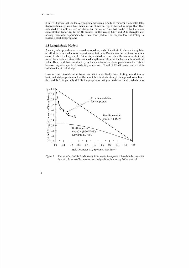
It is well known that the tension and compression strength of composite laminates fallsdisproportionately with hole diameter. As shown in Fig. 1, this fall is larger than thatpredicted by simple net section stress, but not as large as that predicted by the stress
concentration factor (Kt) for brittle failure. For this reason OHT and OHB strengths areusually measured experimentally. These form part of the coupon level of testing inbuilding-block test programs.
1.3 Length Scale Models
A variety of approaches have been developed to predict the effect of holes on strength inan effort to reduce reliance on experimental test data. One class of model incorporates aconcept called the length scale. Failure is predicted to occur when the stress, or strain, atsome characteristic distance, the so called length scale, ahead of the hole reaches a criticalvalue. These models are used widely by the manufacturers of composite aircraft structure
because they are capable of predicting failure in OHT and OHC with an accuracy that issufficient for aircraft design.
However, such models suffer from two deficiencies. Firstly, some testing in addition tobasic material properties such as the unnotched laminate strength is required to calibratethe models. This partially defeats the purpose of using a predictive model, which is to
0.0
0.1
0.2
0.3
0.4
0.5
0.6
0.7
0.8
0.9
1.0
0.0 0.1 0.2 0.3 0.4 0.5 0.6 0.7 0.8 0.9 1.0
Hole Diameter (D)/Specimen Width (W)
N o t c h e d
S t r e n g t h / U n n o t c h e d S t r e n g t h
( σ n / σ 0 )
Ductile material
σn/σ0 = 1-D/W
Brittle material
σn/σ0 = (1-D/W)/KtKt = 2+(1-D/W)^3
Experimental datafor composites
Figure 1: Plot showing that the tensile strength of a notched composite is less than that predicted for a ductile material but greater than that predicted for a purely brittle material

7/31/2019 Effect Hole Size Env Callus DSTO TR 2077
http://slidepdf.com/reader/full/effect-hole-size-env-callus-dsto-tr-2077 13/82
DSTO-TR-2077
3
reduce the amount of testing. Secondly, these models appear not to be applicable once out-of-plane bending loads become significant.
While the dominant loading in well-designed composite aircraft structure is in-plane sothat applied loads may be supported by the strong and stiff fibres, a significant number oflaminates are subjected to significant proportions of out-of-plane loading. For examplemany stiffeners (ribs, hats, stringers, etc.) are flanged and the flange is fastened or bondedto a thin skin. Loads originating in the skin and flowing into the stiffener will createsecondary bending in that stiffener because the fastener holes or bonding surface in theattachment flange are offset from the load-bearing body of the stiffener.
In these cases it is presumed that the in-plane length scale models are not sufficientlyaccurate because manufacturers usually perform additional testing to determine strengthin the presence of significant out-of-plane bending, rather than using these models. One of
the aims of this report is to quantify the extent of this difference by comparing thepredictions from the three commonly used length scale criteria described in Section 2 withexperimentally obtained OHT, OHC and OHB strengths.
2 Selected Length Scale Models
2.1 Average and point stress criteria
Whitney and Nuismer (W-N) [1] developed two criteria to account for the effect of holeson the tensile strength of composite laminates. They are commonly referred to as theAverage Stress Criterion (ASC) and the Point Stress Criterion (PSC). Both were developedto model the situation shown in Fig. 1, where the loss in tensile strength of notchedcomposites was greater than that due to the reduction in net section but less than that dueto a stress concentration factor.
Both of the ASC and PSC require an expression for the stress distribution around the hole.For an infinite orthotropic plate containing a circular hole with a uniform remote stress,
σ∞, applied parallel to the y-axis then the normal stress, σy, along the x-axis in theremaining ligament can be approximated by Equation 1 [2].
( ) ( )⎪⎭
⎪⎬⎫
⎪⎩
⎪⎨⎧
⎥⎥⎦
⎤
⎢⎢⎣
⎡⎟ ⎠
⎞⎜⎝
⎛ ⎟ ⎠
⎞⎜⎝
⎛ ⎟ ⎠
⎞⎜⎝
⎛ ⎟ ⎠
⎞⎜⎝
⎛ = −−−++∞σ
σ ∞86
T
42
yx
r7
x
r53K
x
r3
x
r2
2x,0 (1)
Where:r = radius of holex = distance from edge of hole
∞TK = orthotropic stress concentration factor for a plate of infinite width
7/31/2019 Effect Hole Size Env Callus DSTO TR 2077
http://slidepdf.com/reader/full/effect-hole-size-env-callus-dsto-tr-2077 14/82
DSTO-TR-2077
4
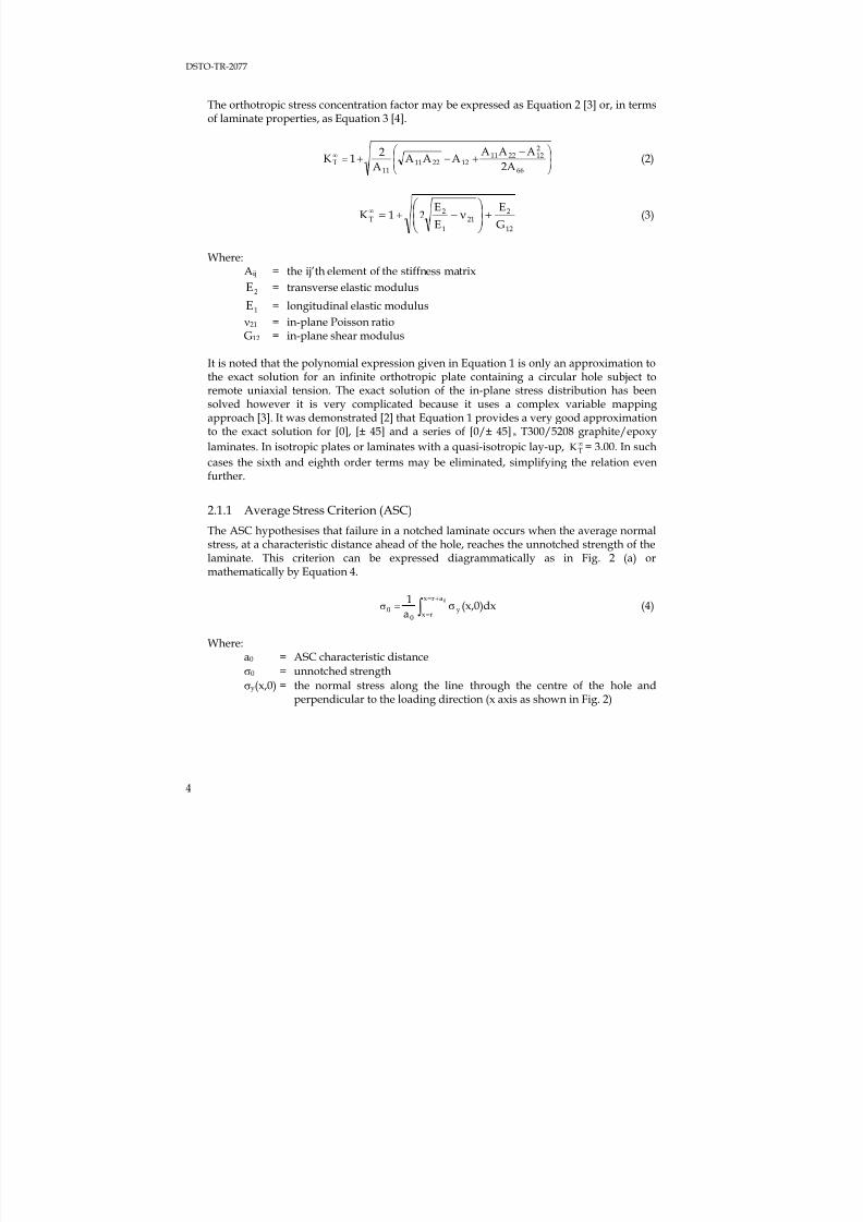
The orthotropic stress concentration factor may be expressed as Equation 2 [3] or, in termsof laminate properties, as Equation 3 [4].
⎟⎟ ⎠ ⎞
⎜⎜⎝ ⎛ = −+−+∞
66
2122211122211
11T 2A
AAAAAAA
21K (2)
12
221
1
2T
G
E
E
E1K +⎟
⎟ ⎠
⎞⎜⎜⎝
⎛ ν−= +∞
2 (3)
Where:Aij = the ij’th element of the stiffness matrix
2E = transverse elastic modulus
1E = longitudinal elastic modulus
ν21 = in-plane Poisson ratioG12 = in-plane shear modulus
It is noted that the polynomial expression given in Equation 1 is only an approximation tothe exact solution for an infinite orthotropic plate containing a circular hole subject toremote uniaxial tension. The exact solution of the in-plane stress distribution has beensolved however it is very complicated because it uses a complex variable mappingapproach [3]. It was demonstrated [2] that Equation 1 provides a very good approximationto the exact solution for [0], [± 45] and a series of [0/± 45] s T300/5208 graphite/epoxy
laminates. In isotropic plates or laminates with a quasi-isotropic lay-up,
∞
TK = 3.00. In suchcases the sixth and eighth order terms may be eliminated, simplifying the relation evenfurther.
2.1.1 Average Stress Criterion (ASC)
The ASC hypothesises that failure in a notched laminate occurs when the average normalstress, at a characteristic distance ahead of the hole, reaches the unnotched strength of thelaminate. This criterion can be expressed diagrammatically as in Fig. 2 (a) ormathematically by Equation 4.
(x,0)dxa10arx
rxy∫
+=
= σ=σ0
0 (4)
Where:a0 = ASC characteristic distance
σ0 = unnotched strength
σy(x,0) = the normal stress along the line through the centre of the hole andperpendicular to the loading direction (x axis as shown in Fig. 2)
7/31/2019 Effect Hole Size Env Callus DSTO TR 2077
http://slidepdf.com/reader/full/effect-hole-size-env-callus-dsto-tr-2077 15/82
DSTO-TR-2077
5
(a) (b)
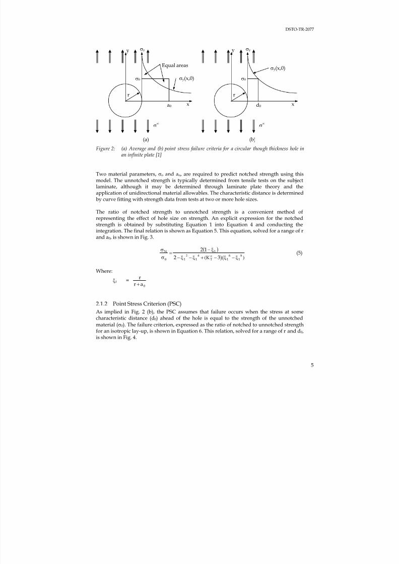
Figure 2: (a) Average and (b) point stress failure criteria for a circular though thickness hole inan infinite plate [1]
Two material parameters, σo and ao, are required to predict notched strength using thismodel. The unnotched strength is typically determined from tensile tests on the subjectlaminate, although it may be determined through laminate plate theory and theapplication of unidirectional material allowables. The characteristic distance is determinedby curve fitting with strength data from tests at two or more hole sizes.
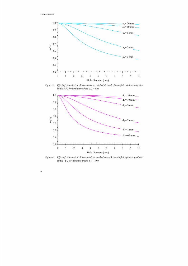
The ratio of notched strength to unnotched strength is a convenient method ofrepresenting the effect of hole size on strength. An explicit expression for the notchedstrength is obtained by substituting Equation 1 into Equation 4 and conducting theintegration. The final relation is shown as Equation 5. This equation, solved for a range of rand a0, is shown in Fig. 3.
( )
)(8642
11T11
1N
3)(2
12
K ξ−ξ−+ξ−ξ−
ξ−=
σ
σ∞
0
(5)
Where:
ξ1 =0ar
r+
2.1.2 Point Stress Criterion (PSC)
As implied in Fig. 2 (b), the PSC assumes that failure occurs when the stress at somecharacteristic distance (d0) ahead of the hole is equal to the strength of the unnotched
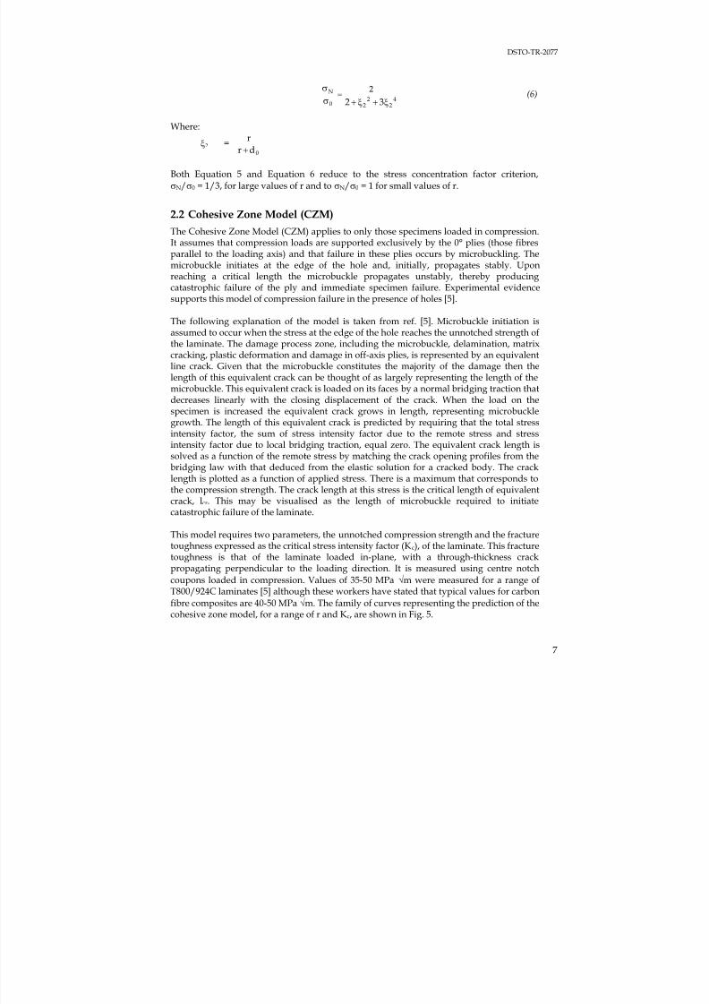
material (σ0). The failure criterion, expressed as the ratio of notched to unnotched strengthfor an isotropic lay-up, is shown in Equation 6. This relation, solved for a range of r and d0,is shown in Fig. 4.
x
σy
r
σ0
d0
σ∞
σy(x,0)
y
x
σy
r
σ0
a0
σ∞
σy(x,0)
y
Equal areas
7/31/2019 Effect Hole Size Env Callus DSTO TR 2077
http://slidepdf.com/reader/full/effect-hole-size-env-callus-dsto-tr-2077 16/82
DSTO-TR-2077
6
Figure 3: Effect of characteristic dimension a0 on notched strength of an infinite plate as predicted
by the ASC for laminates where 00.3=∞T
K
Figure 4: Effect of characteristic dimension d0 on notched strength of an infinite plate as predicted
by the PSC for laminates where 00.3=∞T
K
0.3
0.4
0.5
0.6
0.7
0.8
0.9
1.0
0 1 2 3 4 5 6 7 8 9 10
Hole diameter (mm)
σ N
/ σ 0
d0 = 1 mm
d0 = 2 mm
d0 = 5 mm
d0 = 10 mm
d0 = 20 mm
d0 = 0.5 mm
0.3
0.4
0.5
0.6
0.7
0.8
0.9
1.0
0 1 2 3 4 5 6 7 8 9 10
Hole diameter (mm)
σ N
/ σ 0
a0 = 1 mm
a0 = 2 mm
a0 = 5 mm
a0 = 10 mm
a0 = 20 mm
7/31/2019 Effect Hole Size Env Callus DSTO TR 2077
http://slidepdf.com/reader/full/effect-hole-size-env-callus-dsto-tr-2077 17/82
DSTO-TR-2077
7
42
220
N
32
2
ξ+ξ+σσ
= (6)
Where:
ξ2 =0dr
r
+
Both Equation 5 and Equation 6 reduce to the stress concentration factor criterion,
σN/σ0 = 1/3, for large values of r and to σN/σ0 = 1 for small values of r.
2.2 Cohesive Zone Model (CZM)
The Cohesive Zone Model (CZM) applies to only those specimens loaded in compression.
It assumes that compression loads are supported exclusively by the 0° plies (those fibresparallel to the loading axis) and that failure in these plies occurs by microbuckling. Themicrobuckle initiates at the edge of the hole and, initially, propagates stably. Uponreaching a critical length the microbuckle propagates unstably, thereby producingcatastrophic failure of the ply and immediate specimen failure. Experimental evidencesupports this model of compression failure in the presence of holes [5].
The following explanation of the model is taken from ref. [5]. Microbuckle initiation isassumed to occur when the stress at the edge of the hole reaches the unnotched strength ofthe laminate. The damage process zone, including the microbuckle, delamination, matrixcracking, plastic deformation and damage in off-axis plies, is represented by an equivalentline crack. Given that the microbuckle constitutes the majority of the damage then thelength of this equivalent crack can be thought of as largely representing the length of themicrobuckle. This equivalent crack is loaded on its faces by a normal bridging traction thatdecreases linearly with the closing displacement of the crack. When the load on thespecimen is increased the equivalent crack grows in length, representing microbucklegrowth. The length of this equivalent crack is predicted by requiring that the total stressintensity factor, the sum of stress intensity factor due to the remote stress and stressintensity factor due to local bridging traction, equal zero. The equivalent crack length issolved as a function of the remote stress by matching the crack opening profiles from thebridging law with that deduced from the elastic solution for a cracked body. The cracklength is plotted as a function of applied stress. There is a maximum that corresponds tothe compression strength. The crack length at this stress is the critical length of equivalentcrack, lcr. This may be visualised as the length of microbuckle required to initiatecatastrophic failure of the laminate.
This model requires two parameters, the unnotched compression strength and the fracturetoughness expressed as the critical stress intensity factor (Kc), of the laminate. This fracturetoughness is that of the laminate loaded in-plane, with a through-thickness crackpropagating perpendicular to the loading direction. It is measured using centre notch
coupons loaded in compression. Values of 35-50 MPa √m were measured for a range ofT800/924C laminates [5] although these workers have stated that typical values for carbon
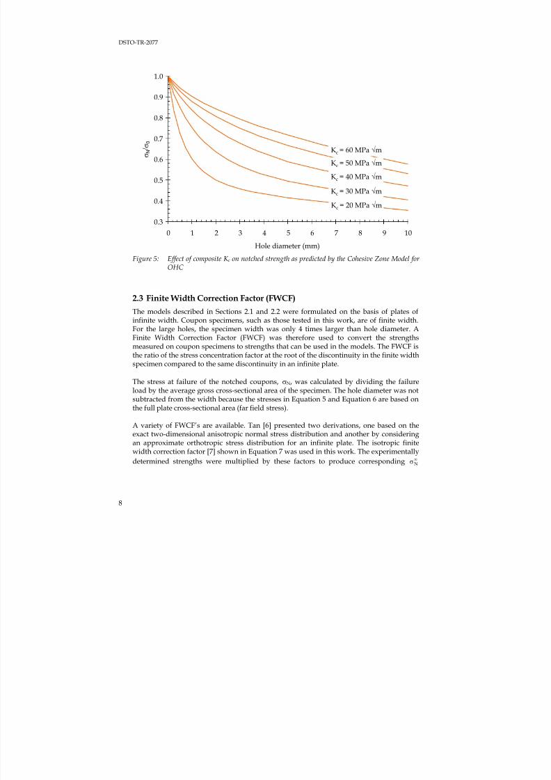
fibre composites are 40-50 MPa √m. The family of curves representing the prediction of thecohesive zone model, for a range of r and Kc, are shown in Fig. 5.
7/31/2019 Effect Hole Size Env Callus DSTO TR 2077
http://slidepdf.com/reader/full/effect-hole-size-env-callus-dsto-tr-2077 18/82
DSTO-TR-2077
8
Figure 5: Effect of composite K c on notched strength as predicted by the Cohesive Zone Model for OHC
2.3 Finite Width Correction Factor (FWCF)
The models described in Sections 2.1 and 2.2 were formulated on the basis of plates ofinfinite width. Coupon specimens, such as those tested in this work, are of finite width.For the large holes, the specimen width was only 4 times larger than hole diameter. AFinite Width Correction Factor (FWCF) was therefore used to convert the strengthsmeasured on coupon specimens to strengths that can be used in the models. The FWCF isthe ratio of the stress concentration factor at the root of the discontinuity in the finite widthspecimen compared to the same discontinuity in an infinite plate.
The stress at failure of the notched coupons,σ
N, was calculated by dividing the failureload by the average gross cross-sectional area of the specimen. The hole diameter was notsubtracted from the width because the stresses in Equation 5 and Equation 6 are based onthe full plate cross-sectional area (far field stress).
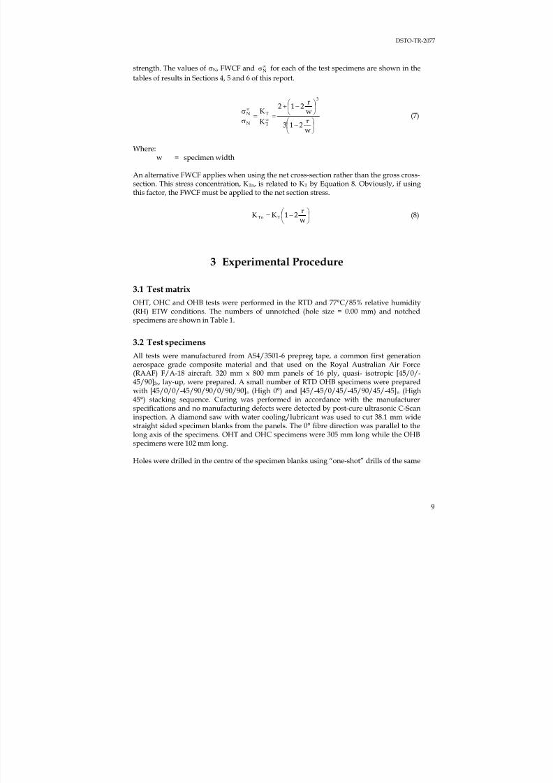
A variety of FWCF’s are available. Tan [6] presented two derivations, one based on theexact two-dimensional anisotropic normal stress distribution and another by consideringan approximate orthotropic stress distribution for an infinite plate. The isotropic finitewidth correction factor [7] shown in Equation 7 was used in this work. The experimentally
determined strengths were multiplied by these factors to produce corresponding ∞σN
0.3
0.4
0.5
0.6
0.7
0.8
0.9
1.0
0 1 2 3 4 5 6 7 8 9 10
Hole diameter (mm)
σ N
/ σ 0
Kc = 20 MPa √m
Kc = 30 MPa √m
Kc = 40 MPa √m
Kc = 50 MPa √m
Kc = 60 MPa √m
7/31/2019 Effect Hole Size Env Callus DSTO TR 2077
http://slidepdf.com/reader/full/effect-hole-size-env-callus-dsto-tr-2077 19/82
DSTO-TR-2077
9
strength. The values of σN, FWCF and ∞σN for each of the test specimens are shown in the
tables of results in Sections 4, 5 and 6 of this report.
⎟ ⎠
⎞⎜⎝
⎛
⎟ ⎠
⎞⎜⎝
⎛
=
−
−+=
σσ
∞
∞
w
r213
w
r212
K
K
3
T
T
N
N (7)
Where:w = specimen width
An alternative FWCF applies when using the net cross-section rather than the gross cross-section. This stress concentration, KTn, is related to KT by Equation 8. Obviously, if using
this factor, the FWCF must be applied to the net section stress.
⎟ ⎠
⎞⎜⎝
⎛ −=w
r21KK TTn (8)
3 Experimental Procedure
3.1 Test matrixOHT, OHC and OHB tests were performed in the RTD and 77°C/85% relative humidity(RH) ETW conditions. The numbers of unnotched (hole size = 0.00 mm) and notchedspecimens are shown in Table 1.
3.2 Test specimens
All tests were manufactured from AS4/3501-6 prepreg tape, a common first generationaerospace grade composite material and that used on the Royal Australian Air Force(RAAF) F/A-18 aircraft. 320 mm x 800 mm panels of 16 ply, quasi- isotropic [45/0/-45/90]2s, lay-up, were prepared. A small number of RTD OHB specimens were preparedwith [45/0/0/-45/90/90/0/90/90]s (High 0°) and [45/-45/0/45/-45/90/45/-45]s (High45°) stacking sequence. Curing was performed in accordance with the manufacturerspecifications and no manufacturing defects were detected by post-cure ultrasonic C-Scaninspection. A diamond saw with water cooling/lubricant was used to cut 38.1 mm widestraight sided specimen blanks from the panels. The 0° fibre direction was parallel to thelong axis of the specimens. OHT and OHC specimens were 305 mm long while the OHBspecimens were 102 mm long.
Holes were drilled in the centre of the specimen blanks using “one-shot” drills of the same
7/31/2019 Effect Hole Size Env Callus DSTO TR 2077
http://slidepdf.com/reader/full/effect-hole-size-env-callus-dsto-tr-2077 20/82
DSTO-TR-2077
10
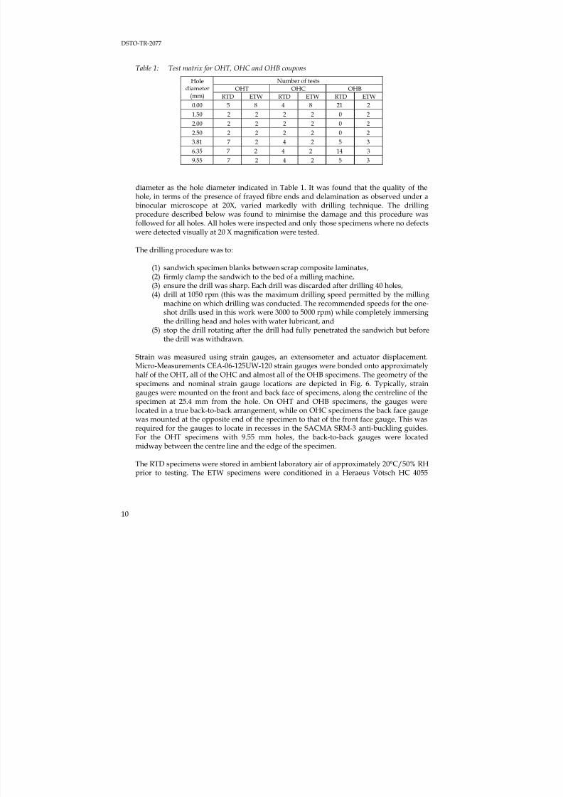
Table 1: Test matrix for OHT, OHC and OHB coupons
Number of tests
OHT OHC OHBHole
diameter
(mm) RTD ETW RTD ETW RTD ETW0.00 5 8 4 8 21 2
1.50 2 2 2 2 0 2
2.00 2 2 2 2 0 2
2.50 2 2 2 2 0 2
3.81 7 2 4 2 5 3
6.35 7 2 4 2 14 3
9.55 7 2 4 2 5 3
diameter as the hole diameter indicated in Table 1. It was found that the quality of the
hole, in terms of the presence of frayed fibre ends and delamination as observed under abinocular microscope at 20X, varied markedly with drilling technique. The drillingprocedure described below was found to minimise the damage and this procedure wasfollowed for all holes. All holes were inspected and only those specimens where no defectswere detected visually at 20 X magnification were tested.
The drilling procedure was to:
(1) sandwich specimen blanks between scrap composite laminates,(2) firmly clamp the sandwich to the bed of a milling machine,(3) ensure the drill was sharp. Each drill was discarded after drilling 40 holes,
(4) drill at 1050 rpm (this was the maximum drilling speed permitted by the millingmachine on which drilling was conducted. The recommended speeds for the one-shot drills used in this work were 3000 to 5000 rpm) while completely immersingthe drilling head and holes with water lubricant, and
(5) stop the drill rotating after the drill had fully penetrated the sandwich but beforethe drill was withdrawn.
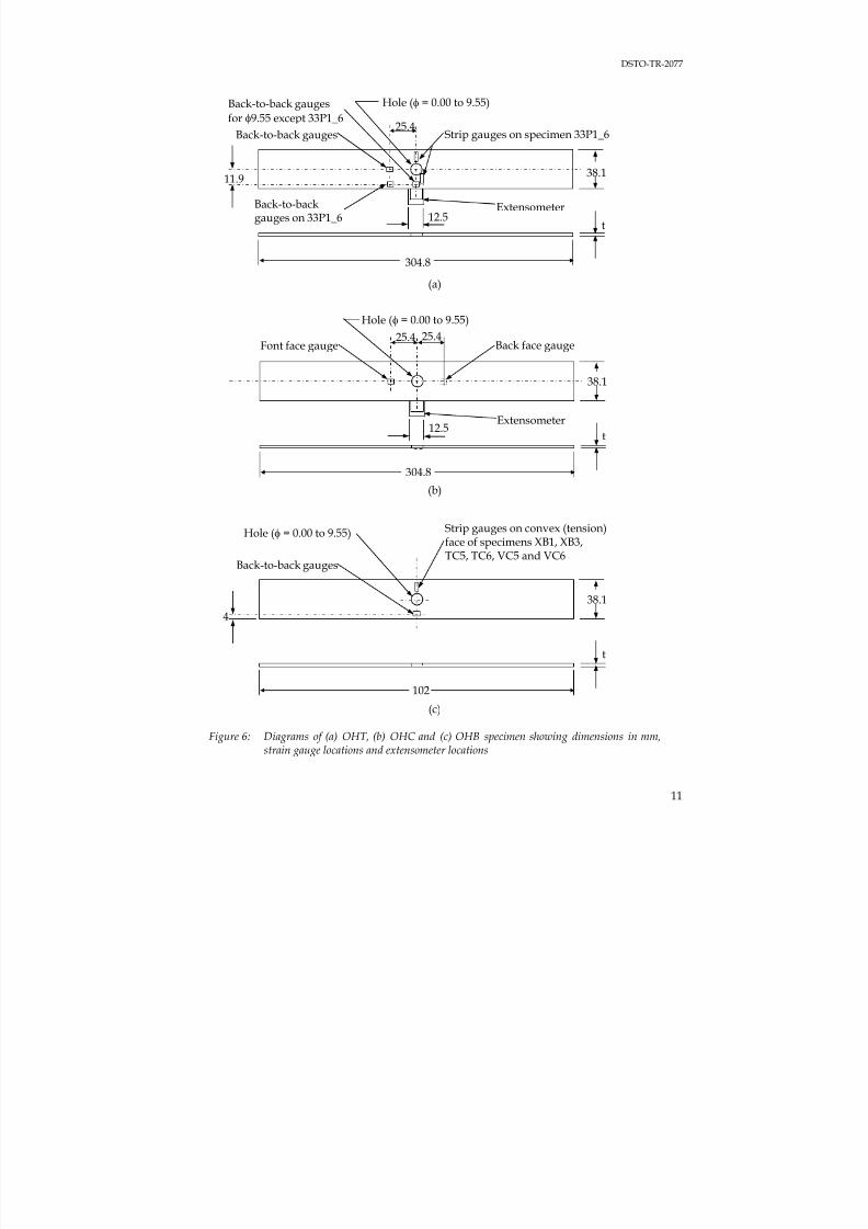
Strain was measured using strain gauges, an extensometer and actuator displacement.Micro-Measurements CEA-06-125UW-120 strain gauges were bonded onto approximatelyhalf of the OHT, all of the OHC and almost all of the OHB specimens. The geometry of thespecimens and nominal strain gauge locations are depicted in Fig. 6. Typically, strain
gauges were mounted on the front and back face of specimens, along the centreline of thespecimen at 25.4 mm from the hole. On OHT and OHB specimens, the gauges werelocated in a true back-to-back arrangement, while on OHC specimens the back face gaugewas mounted at the opposite end of the specimen to that of the front face gauge. This wasrequired for the gauges to locate in recesses in the SACMA SRM-3 anti-buckling guides.For the OHT specimens with 9.55 mm holes, the back-to-back gauges were locatedmidway between the centre line and the edge of the specimen.
The RTD specimens were stored in ambient laboratory air of approximately 20°C/50% RHprior to testing. The ETW specimens were conditioned in a Heraeus Vötsch HC 4055
7/31/2019 Effect Hole Size Env Callus DSTO TR 2077
http://slidepdf.com/reader/full/effect-hole-size-env-callus-dsto-tr-2077 21/82
DSTO-TR-2077
11
(a)
(b)
(c)
Figure 6: Diagrams of (a) OHT, (b) OHC and (c) OHB specimen showing dimensions in mm,strain gauge locations and extensometer locations
25.4 25.4Font face gauge Back face gauge
38.1
t12.5
Extensometer
304.8
Hole (φ = 0.00 to 9.55)
25.4
Back-to-back gauges
for φ9.55 except 33P1_6
38.1
t12.5
Extensometer
304.8
Strip gauges on specimen 33P1_6
11.9
Back-to-backgauges on 33P1_6
Hole (φ = 0.00 to 9.55)
Back-to-back gauges
38.1
t
102
Strip gauges on convex (tension)face of specimens XB1, XB3,TC5, TC6, VC5 and VC6
4
Hole (φ = 0.00 to 9.55)
Back-to-back gauges
7/31/2019 Effect Hole Size Env Callus DSTO TR 2077
http://slidepdf.com/reader/full/effect-hole-size-env-callus-dsto-tr-2077 22/82
DSTO-TR-2077
12
environmental chamber at 70°C/85% RH. The moisture content of the specimens wasmonitored by measuring weight gain. Conditioning was considered complete when theweight gain in specimens was less that 0.05% for consecutive readings taken 7 days apart.
Strip gauges were bonded to one of the OHT and six of the OHB specimens in thelocations shown in Fig. 6. The strip gauges consisted of five individual gauges, each with agauge length of 1.5 mm and a pitch (centre-to-centre separation) of 2.0 mm. These wereused to measure the strain distribution along the ligament between the edge of the holeand the specimen edge.
A MTS 632 series extensometer with a 12.5 mm gauge length was attached to one RTDOHT and OHC specimen of each hole size at the location shown in Fig. 6.
No end tabs were used on any of the specimens. Prior to testing, the thickness and width
of the test section was measured in three locations.
3.3 Test procedure
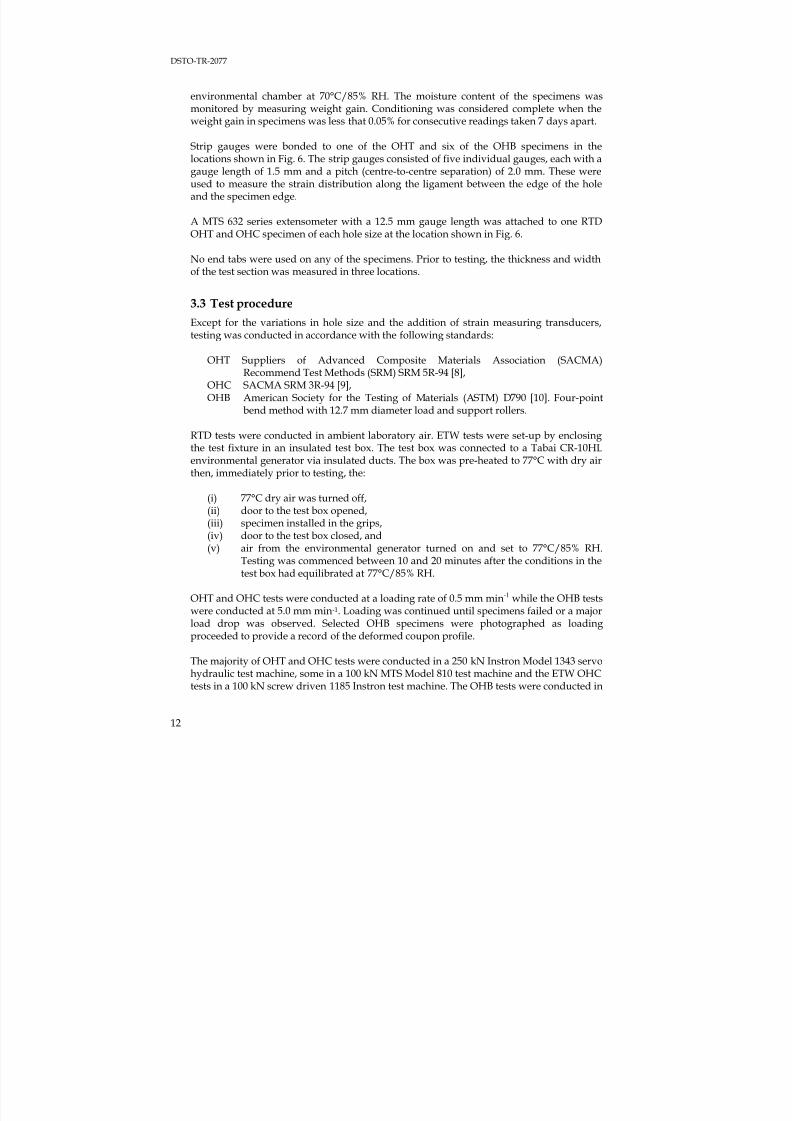
Except for the variations in hole size and the addition of strain measuring transducers,testing was conducted in accordance with the following standards:
OHT Suppliers of Advanced Composite Materials Association (SACMA)Recommend Test Methods (SRM) SRM 5R-94 [8],
OHC SACMA SRM 3R-94 [9],OHB American Society for the Testing of Materials (ASTM) D790 [10]. Four-point
bend method with 12.7 mm diameter load and support rollers.
RTD tests were conducted in ambient laboratory air. ETW tests were set-up by enclosingthe test fixture in an insulated test box. The test box was connected to a Tabai CR-10HLenvironmental generator via insulated ducts. The box was pre-heated to 77°C with dry airthen, immediately prior to testing, the:
(i) 77°C dry air was turned off,(ii) door to the test box opened,(iii) specimen installed in the grips,(iv) door to the test box closed, and
(v)
air from the environmental generator turned on and set to 77°C/85% RH.Testing was commenced between 10 and 20 minutes after the conditions in thetest box had equilibrated at 77°C/85% RH.
OHT and OHC tests were conducted at a loading rate of 0.5 mm min-1 while the OHB testswere conducted at 5.0 mm min-1. Loading was continued until specimens failed or a majorload drop was observed. Selected OHB specimens were photographed as loadingproceeded to provide a record of the deformed coupon profile.
The majority of OHT and OHC tests were conducted in a 250 kN Instron Model 1343 servohydraulic test machine, some in a 100 kN MTS Model 810 test machine and the ETW OHCtests in a 100 kN screw driven 1185 Instron test machine. The OHB tests were conducted in
7/31/2019 Effect Hole Size Env Callus DSTO TR 2077
http://slidepdf.com/reader/full/effect-hole-size-env-callus-dsto-tr-2077 23/82
DSTO-TR-2077
13
the 1185 Instron. The MTS machines were fitted with hydraulic grips while the Instronwas fitted with flat compression platens for OHC tests and a four point bend fixture forthe OHB testing. It was assumed that the change in test machine had no effect on the test
results.
Personal computer based data acquisition systems were used. For each test the machineload, actuator displacement and strains from the strain gauges and extensometer wererecorded.
4 Results and Discussion - Tension
4.1 Stress-strain behaviour
4.1.1 Strain gauge
The stress-strain response of RTD and ETW specimens was expected, and observed, to belinear to failure. All transducers for the RTD, and the extensometer and actuatordisplacement for the ETW, specimens were linear as shown in Fig. 7.
The strain gauge response for 12 of the 20 ETW specimens was unexpectedly non-linear,with some apparent stiffening. A typical example is shown in Fig. 7. The likely explanationfor this apparent strain stiffening was reorientation of fibres in the surface plies toward the
direction of the loading axis. It is hypothesised that the fibres in the outer 45° ply, to whichthe strain gauges were bonded, rotated sufficiently during testing to cause the apparentstiffening. Supporting this claim are the observations that the plies (i) were only supportedon their back face thus less restrained from rotating as the test progressed, (ii) experienceda significant component of load in the direction of the loading axis, and (iii) weresupported by a relatively soft matrix in the ETW condition. A similar phenomenon, wherethe tows in woven composites straightened at high load (termed plastic tow straightening)has been reported elsewhere [11].
Two observations that further support the hypothesis of fibre rotation in the outer ply arethat, firstly, the strain gauge measurements initially matched those of the extensometer
and only began deviating from linearity after the load had exceeded the yield strength ofthe matrix (yield strength ≈ 70 MPa, deviation commenced ≈ 120 MPa). Secondly, a veryfine feathering was observed on the edges of some of the ETW specimens after testing.
This feathering was of the same type as that found on the edges of failed ±45° tensionspecimens, where plies are known to disbond and move in a “scissor” action duringtesting. This contrasted with failed RTD specimens where the edges were almost assmooth as prior to the testing.

7/31/2019 Effect Hole Size Env Callus DSTO TR 2077
http://slidepdf.com/reader/full/effect-hole-size-env-callus-dsto-tr-2077 24/82
DSTO-TR-2077
14
Figure 7: Typical stress-strain response from a RTD (0.00 mm hole, specimen 33p2_13) andETW (1.50 mm hole, specimen JC3) specimen. Both the strain gauge and extensometer data are shown for the ETW specimen
The strain measured by the extensometer, even on the ETW specimens, was not expectedto exhibit this apparent stiffening because the extensometer was located on the edge of thespecimen and so measured the averaged strain through-the-thickness of the specimen.This averaged strain was dominated by the behaviour of the 0° plies, where any fibrerotation would be very small.
The response of the back-to-back gauges in both the RTD and ETW specimens diverged,indicating bending in these specimens. There was no bending limit prescribed in ASTM D3039, however it recommended that to be consistent with good testing practice thebending should be limited to 3-5%. The average bending, calculated at the maximum loadthat the back-to-back gauges functioned reliably, was 1.3% for RTD and 5.0% for ETW,indicating an acceptable level of bending.
4.1.2 Extensometer
An extensometer was used to measure the displacement across the hole on some RTDspecimens and on all of the ETW specimens. The results were very similar to those shownin Fig. 7. There was very little difference in the strains measured by the strain gauge andextensometer on RTD specimens. The strains measured by the extensometer weretherefore used for further analysis. In contrast, the ETW extensometer response was linearto failure whereas the strain gauges exhibited the apparent stiffening. As indicated inSection 4.1.1, the non-linear response of the strain gauges was judged to not be a true
0
100
200
300
400
500
600
700
0 2000 4000 6000 8000 10000 12000 14000
Strain (microstrain)
G r o s s s e c t i o n s t r e s s ( M P a )
RTD (0.00 hole)
back-to-back
strain gauges
ETW (1.50 hole)back-to-back
strain gauges
ETW (1.50 hole)
front-face
extensometer
7/31/2019 Effect Hole Size Env Callus DSTO TR 2077
http://slidepdf.com/reader/full/effect-hole-size-env-callus-dsto-tr-2077 25/82
DSTO-TR-2077
15
reflection of material behaviour. Therefore the extensometer data was used for analyses ofETW OHT behaviour.
4.1.3 Actuator
A technique was developed to calibrate the strains calculated from displacement of the testmachine actuator with those from the strain gauge. This allowed strains to be estimated inthose specimens where no strain gauges were installed or where there were obvious errorsin the strain gauge data. The calibration process is described in detail in Appendix A. Insummary, the approach was to; calculate a nominal strain from the actuator displacement,factor this strain so that it matched the strain measured by strain gauges, account for theoffset at zero load then correct for deformation of the load-train.
The correlations obtained using this approach appeared to be very good. For 22 RTD OHT
specimens where reliable data from both strain gauges and the actuator were available, theaverage difference in failure strain as determined by the strain gauge and corrected
actuator displacement was 260 με. This value was skewed by large errors in two
specimens. Ignoring these outliers reduced the typical difference to 170 με, which wasequivalent to less than 2% of the failure strain, well within the experimental scatter ofresults. Similarly, for the 9 ETW OHT specimens where reliable extensometer andcorrected actuator displacement data was available, the average difference in failure
strains was 75 με or less than 1 % of the failure strain. Again, this was an excellent match.
4.1.4 Stress-strain behaviour
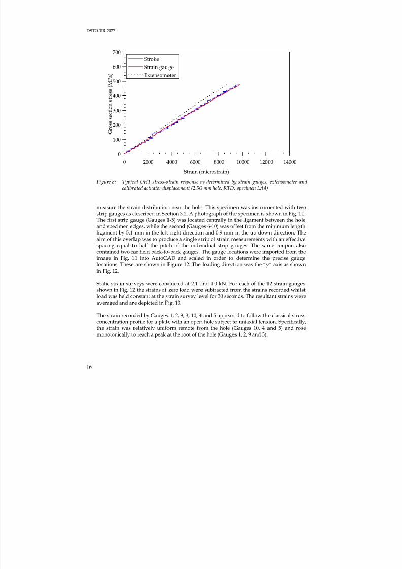
In a few cases the response from strain gauge, extensometer and actuator displacementsmatched. For most specimens there was a gradual deviation of one of the transducers, atypical result being shown in Fig. 8. The hierarchy shown in Table 2 was thereforedeveloped to select which strain transducer would be used for further analysis. Unlessstated otherwise the OHT strain data was obtained from the most preferred transducerindicated in Table 2.
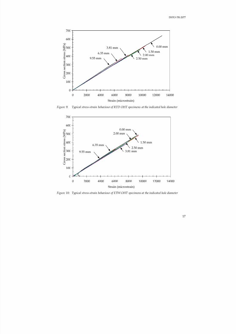
Typical stress-strain behaviour for each of the hole sizes are shown in Figs 9 and 10. The
elastic modulus from 1000 to 3000 με, failure strength and strain were determined usingthe most preferred data source available and the approaches described in Sections 4.3 to4.5. These data are shown in Tables 3 and 4.
4.2 Strain distribution
A strain survey was conducted on a RTD specimen with a 9.55 mm hole (33P1_6) to
Table 2: Hierarchy of strain transducers for OHT testsPriority RTD ETW
Most preferred average back-to-back strain gauge extensometer
Second preferred extensometer actuator displacement
Least preferred actuator displacement average back-to-back strain gauge
7/31/2019 Effect Hole Size Env Callus DSTO TR 2077
http://slidepdf.com/reader/full/effect-hole-size-env-callus-dsto-tr-2077 26/82
DSTO-TR-2077
16
Figure 8: Typical OHT stress-strain response as determined by strain gauges, extensometer andcalibrated actuator displacement (2.50 mm hole, RTD, specimen LA4)
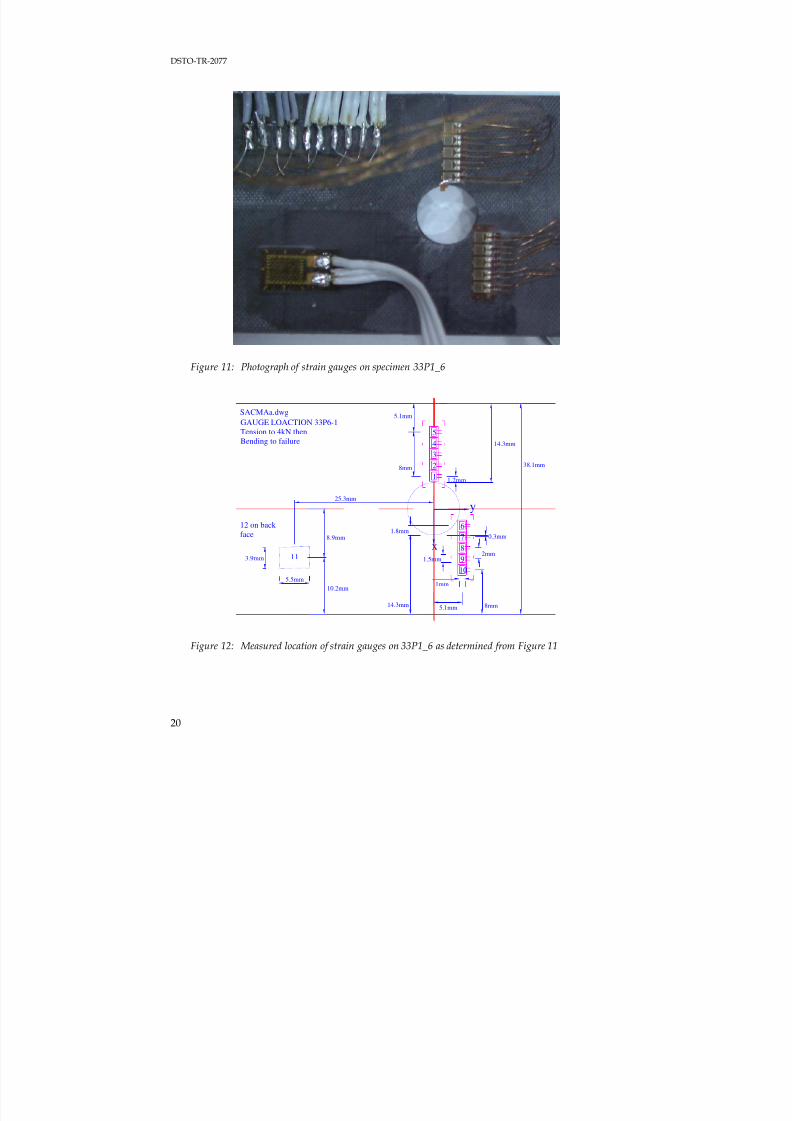
measure the strain distribution near the hole. This specimen was instrumented with twostrip gauges as described in Section 3.2. A photograph of the specimen is shown in Fig. 11.The first strip gauge (Gauges 1-5) was located centrally in the ligament between the holeand specimen edges, while the second (Gauges 6-10) was offset from the minimum lengthligament by 5.1 mm in the left-right direction and 0.9 mm in the up-down direction. Theaim of this overlap was to produce a single strip of strain measurements with an effectivespacing equal to half the pitch of the individual strip gauges. The same coupon alsocontained two far field back-to-back gauges. The gauge locations were imported from theimage in Fig. 11 into AutoCAD and scaled in order to determine the precise gaugelocations. These are shown in Figure 12. The loading direction was the “y” axis as shownin Fig. 12.
Static strain surveys were conducted at 2.1 and 4.0 kN. For each of the 12 strain gaugesshown in Fig. 12 the strains at zero load were subtracted from the strains recorded whilstload was held constant at the strain survey level for 30 seconds. The resultant strains wereaveraged and are depicted in Fig. 13.
The strain recorded by Gauges 1, 2, 9, 3, 10, 4 and 5 appeared to follow the classical stressconcentration profile for a plate with an open hole subject to uniaxial tension. Specifically,the strain was relatively uniform remote from the hole (Gauges 10, 4 and 5) and rosemonotonically to reach a peak at the root of the hole (Gauges 1, 2, 9 and 3).
0
100
200
300
400
500
600
700
0 2000 4000 6000 8000 10000 12000 14000
Strain (microstrain)
G r o s s s e c t i o n s t r e s s ( M P a )
Stroke
Strain gaugeExtensometer
7/31/2019 Effect Hole Size Env Callus DSTO TR 2077
http://slidepdf.com/reader/full/effect-hole-size-env-callus-dsto-tr-2077 27/82
DSTO-TR-2077
17
Figure 9: Typical stress-strain behaviour of RTD OHT specimens at the indicated hole diameter
Figure 10: Typical stress-strain behaviour of ETW OHT specimens at the indicated hole diameter
0
100
200
300
400
500
600
700
0 2000 4000 6000 8000 10000 12000 14000
Strain (microstrain)
G r o s s s e c t i o n s t r e s s ( M P a )
1.50 mm
2.50 mm
3.81 mm
6.35 mm
9.55 mm
0.00 mm
2.00 mm
0
100
200
300
400
500
600
700
0 2000 4000 6000 8000 10000 12000 14000
Strain (microstrain)
G r o s s s e c t i o n s t r e s s ( M P a )
1.50 mm
2.50 mm3.81 mm
6.35 mm
9.55 mm
2.00 mm
0.00 mm
7/31/2019 Effect Hole Size Env Callus DSTO TR 2077
http://slidepdf.com/reader/full/effect-hole-size-env-callus-dsto-tr-2077 28/82
DSTO-TR-2077
18
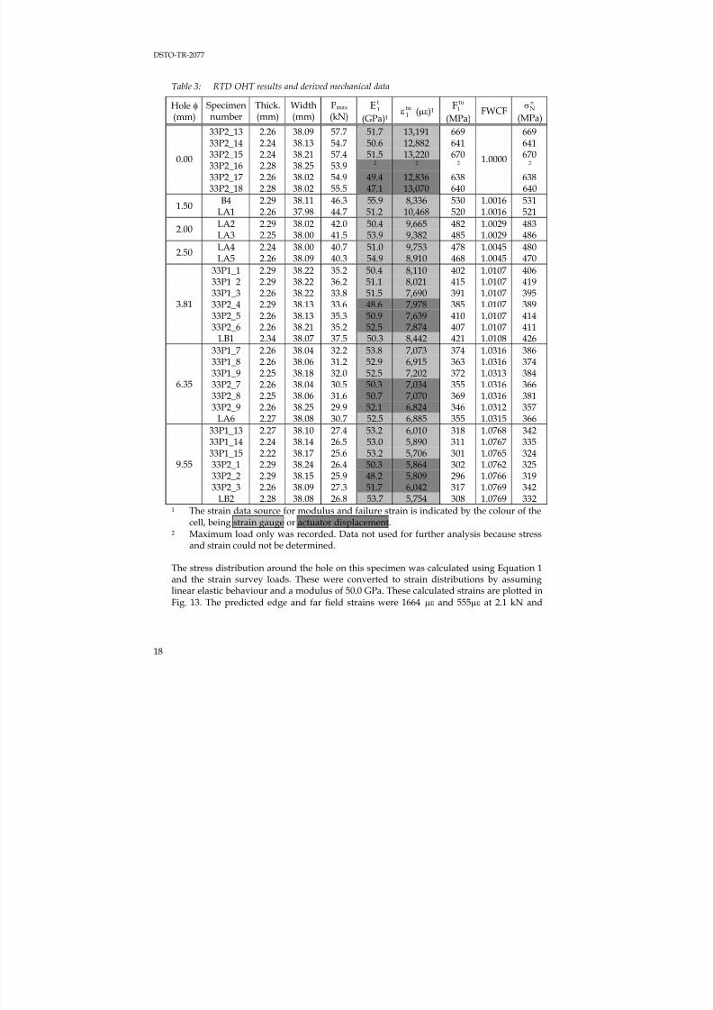
Table 3: RTD OHT results and derived mechanical data
Hole φ (mm)
Specimennumber
Thick.(mm)
Width(mm)
Pmax (kN)
t1E
(GPa)1 tu1ε (με)1
tu1F
(MPa)FWCF
∞σN
(MPa)
33P2_13 2.26 38.09 57.7 51.7 13,191 669 66933P2_14 2.24 38.13 54.7 50.6 12,882 641 64133P2_15 2.24 38.21 57.4 51.5 13,220 670 67033P2_16 2.28 38.25 53.9 2 2 2 2 33P2_17 2.26 38.02 54.9 49.4 12,836 638 638
0.00
33P2_18 2.28 38.02 55.5 47.1 13,070 640
1.0000
640
B4 2.29 38.11 46.3 55.9 8,336 530 1.0016 5311.50
LA1 2.26 37.98 44.7 51.2 10,468 520 1.0016 521
LA2 2.29 38.02 42.0 50.4 9,665 482 1.0029 4832.00
LA3 2.25 38.00 41.5 53.9 9,382 485 1.0029 486
LA4 2.24 38.00 40.7 51.0 9,753 478 1.0045 4802.50LA5 2.26 38.09 40.3 54.9 8,910 468 1.0045 470
33P1_1 2.29 38.22 35.2 50.4 8,110 402 1.0107 40633P1_2 2.29 38.22 36.2 51.1 8,021 415 1.0107 41933P1_3 2.26 38.22 33.8 51.5 7,690 391 1.0107 39533P2_4 2.29 38.13 33.6 48.6 7,978 385 1.0107 38933P2_5 2.26 38.13 35.3 50.9 7,639 410 1.0107 41433P2_6 2.26 38.21 35.2 52.5 7,874 407 1.0107 411
3.81
LB1 2.34 38.07 37.5 50.3 8,442 421 1.0108 426
33P1_7 2.26 38.04 32.2 53.8 7,073 374 1.0316 38633P1_8 2.26 38.06 31.2 52.9 6,915 363 1.0316 374
33P1_9 2.25 38.18 32.0 52.5 7,202 372 1.0313 38433P2_7 2.26 38.04 30.5 50.3 7,034 355 1.0316 36633P2_8 2.25 38.06 31.6 50.7 7,070 369 1.0316 38133P2_9 2.26 38.25 29.9 52.1 6,824 346 1.0312 357
6.35
LA6 2.27 38.08 30.7 52.5 6,885 355 1.0315 366
33P1_13 2.27 38.10 27.4 53.2 6,010 318 1.0768 34233P1_14 2.24 38.14 26.5 53.0 5,890 311 1.0767 33533P1_15 2.22 38.17 25.6 53.2 5,706 301 1.0765 32433P2_1 2.29 38.24 26.4 50.3 5,864 302 1.0762 32533P2_2 2.29 38.15 25.9 48.2 5,809 296 1.0766 31933P2_3 2.26 38.09 27.3 51.7 6,042 317 1.0769 342
9.55
LB2 2.28 38.08 26.8 53.7 5,754 308 1.0769 3321 The strain data source for modulus and failure strain is indicated by the colour of the
cell, being strain gauge or actuator displacement.2 Maximum load only was recorded. Data not used for further analysis because stress
and strain could not be determined.
The stress distribution around the hole on this specimen was calculated using Equation 1and the strain survey loads. These were converted to strain distributions by assuminglinear elastic behaviour and a modulus of 50.0 GPa. These calculated strains are plotted inFig. 13. The predicted edge and far field strains were 1664 με and 555με at 2.1 kN and

7/31/2019 Effect Hole Size Env Callus DSTO TR 2077
http://slidepdf.com/reader/full/effect-hole-size-env-callus-dsto-tr-2077 29/82
DSTO-TR-2077
19
Table 4: ETW OHT results and derived mechanical data
Hole φ (mm)
Specnno.
Thick.(mm)
Width(mm)
Moisture (%)
Pmax (kN)
t1E
(GPa) 1 tu1ε (με)1
tu1F
(MPa)FWCF
∞σN
(MPa)
JA1 2.56 38.08 1.42 44.092 53.0 10,0932 4532 4532 JA2 2.35 38.16 1.58 43.902 54.9 9,3632 4902 4902 NB1 2.30 37.96 1.08 55.04 51.0 13,083 631 631NB2 2.30 37.99 1.07 53.17 53.8 13,891 610 610NB3 2.31 38.02 1.02 46.652 50.7 10,7762 5312 5312 NB4 2.29 38.05 1.04 56.68 53.3 12,120 649 649NB5 2.33 38.01 1.05 55.96 52.2 11,636 632 632
0.00
NB6 2.31 37.98 1.05 55.85 50.6 13,330 636
1.0000
636
JC3 2.43 38.21 1.29 44.88 52.7 9,433 484 1.0016 4851.50
JC4 2.39 38.22 1.33 44.56 54.1 9,332 487 1.0016 488
JC4C 2.40 38.28 1.35 43.24 53.1 8,989 470 1.0028 4712.00 JP6 2.44 38.17 1.36 39.36 51.0 8,421 423 1.0028 424
GC3 2.40 38.19 1.40 39.90 50.9 8,468 435 1.0045 4352.50
JB4 2.41 38.29 1.36 38.11 50.7 7,997 413 1.0045 415
GB6 2.44 38.01 1.39 35.38 50.5 7,715 425 1.0108 4303.81
JB2 2.43 38.19 1.31 35.94 50.8 7,755 387 1.0107 391
GB5 2.44 38.03 1.39 29.67 53.2 6,116 320 1.0316 3306.35
JA6 2.39 38.24 1.33 31.28 53.0 6,647 343 1.0312 354
GA6 2.41 38.03 1.35 27.40 63.9 4,612 299 1.0772 3229.55
GB3 2.42 38.03 1.34 27.49 53.1 5,659 298 1.0772 3211 The strain data source for modulus and failure strain is indicated by the colour of the
cell, being strain gauge, actuator displacement or extensometer.2 Premature specimen failure. This data not used.
3170 με and 1057 με at 4.0 kN respectively. The experimental data conformed very closelywith the predictions of Equation 1, as indicated by a coefficient of determination(R2) = 0.97. R2 was calculated using the method shown in Appendix B.
It was noted that the strains from Gauge 11 were 11% lower (498 με compared to 555 με at2.1 kN and 948 με compared to 1057 με at 4.0 kN) than the far field strains observed inGauges 4 and 5 and predicted by Equation 1. As this gauge was located well outside the
wake of the hole it is unlikely that this discrepancy was caused by the hole shieldingGauge 11 from the full far-field stresses. Conducting the work to explain this discrepancywas beyond the scope of this report.
The response of Gauges 7 and 8 were much lower than predicted by Equation 1. The5.1 mm shift along the y axis (Fig. 12) clearly removed these gauges from the peak strainligament between the hole and the specimen edge. Thus the measurements from thesegauges were not considered representative of the strain profile in the ligament (along the xaxis in Fig. 12). The strain in Gauge 6 was actually lower than that in the far field. This isconsistent with the gauge being in the wake behind the hole where the stressconcentration factor Kt = -1 at the point x=0, y=r.
7/31/2019 Effect Hole Size Env Callus DSTO TR 2077
http://slidepdf.com/reader/full/effect-hole-size-env-callus-dsto-tr-2077 30/82
DSTO-TR-2077
20
Figure 11: Photograph of strain gauges on specimen 33P1_6
1.2mm
0.3mm1.8mm
2mm
5.1mm
1.5mm
38.1mm
10.2mm
8.9mm
25.3mm
8mm14.3mm
14.3mm
5.1mm
8mm
1mm5.5mm
3.9mm
5
4
3
2
1
6
10
7
8
9
SACMAa.dwgGAUGE LOACTION 33P6-1
Tension to 4kN then
Bending to failure
y
x11
12 on back
face
Figure 12: Measured location of strain gauges on 33P1_6 as determined from Figure 11

7/31/2019 Effect Hole Size Env Callus DSTO TR 2077
http://slidepdf.com/reader/full/effect-hole-size-env-callus-dsto-tr-2077 31/82
DSTO-TR-2077
21
Figure 13: Strains in the y direction. Data for 2.1 kN is shown as triangles and 4.0 kN as squares.Each data point is labelled with the strain gauge number. The curves are theoreticalstrains calculated using Equation (1)
4.3 Failure locus
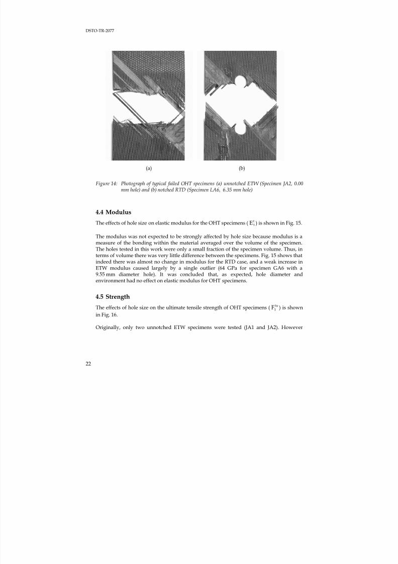
The failed specimens were inspected visually and found to contain significantdelamination with very little fibre pullout. There was no apparent difference between theRTD and ETW specimens as shown by the typical failures in Fig. 14.
The notched coupons failed close to the direct line between the edge of the hole and theclosest specimen edge. Clearly the stress concentration effects of the hole were sufficient toproduce local failure in the load bearing 0° fibres. The delaminations in these specimenswere up to approximately 10 mm long and were present between many of the plies oneach side of the separated specimen halves. The most obvious delamination was thesurface 45° ply. On every specimen this ply separated from the edge of the hole out to theedge of the specimen.
Most of the unnotched coupons failed at or near the grips. This was expected because ofthe stress concentration created by the hard grips on the relatively soft composite. Theunnotched strength data in Tables 3 and 4 must therefore be considered a lower bound.
0
500
1000
1500
2000
2500
3000
3500
-2 -1 0 1 2 3 4 5 6 7 8 9 10
Distance from hole edge (mm)
S t r a i n ( m i c r o s t r a i n )
6
7
1
82
93 10
4
5
11
6
7
1
8 2
11
93 10
4
5
7/31/2019 Effect Hole Size Env Callus DSTO TR 2077
http://slidepdf.com/reader/full/effect-hole-size-env-callus-dsto-tr-2077 32/82
DSTO-TR-2077
22
(a) (b)
Figure 14: Photograph of typical failed OHT specimens (a) unnotched ETW (Specimen JA2, 0.00mm hole) and (b) notched RTD (Specimen LA6, 6.35 mm hole)
4.4 Modulus
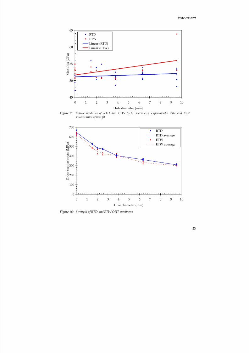
The effects of hole size on elastic modulus for the OHT specimens ( t1E ) is shown in Fig. 15.
The modulus was not expected to be strongly affected by hole size because modulus is ameasure of the bonding within the material averaged over the volume of the specimen.The holes tested in this work were only a small fraction of the specimen volume. Thus, interms of volume there was very little difference between the specimens. Fig. 15 shows thatindeed there was almost no change in modulus for the RTD case, and a weak increase inETW modulus caused largely by a single outlier (64 GPa for specimen GA6 with a9.55 mm diameter hole). It was concluded that, as expected, hole diameter and
environment had no effect on elastic modulus for OHT specimens.
4.5 Strength
The effects of hole size on the ultimate tensile strength of OHT specimens ( tu1F ) is shown
in Fig. 16.
Originally, only two unnotched ETW specimens were tested (JA1 and JA2). However
7/31/2019 Effect Hole Size Env Callus DSTO TR 2077
http://slidepdf.com/reader/full/effect-hole-size-env-callus-dsto-tr-2077 33/82
DSTO-TR-2077
23
Figure 15: Elastic modulus of RTD and ETW OHT specimens, experimental data and leastsquares lines of best fit
Figure 16: Strength of RTD and ETW OHT specimens
45
50
55
60
65
0 1 2 3 4 5 6 7 8 9 10
Hole diameter (mm)
M o d u l u s ( G P a )
RTD
ETW
Linear (RTD)Linear (ETW)
0
100
200
300
400
500
600
700
0 1 2 3 4 5 6 7 8 9 10
Hole diameter (mm)
G r o s s s e c t i o n s t r e s s ( M P a )
RTDRTD average
ETW
ETW average
7/31/2019 Effect Hole Size Env Callus DSTO TR 2077
http://slidepdf.com/reader/full/effect-hole-size-env-callus-dsto-tr-2077 34/82
7/31/2019 Effect Hole Size Env Callus DSTO TR 2077
http://slidepdf.com/reader/full/effect-hole-size-env-callus-dsto-tr-2077 35/82
DSTO-TR-2077
25
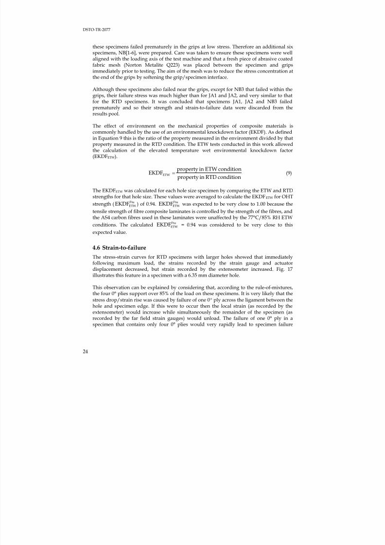
Figure 17: Failure behaviour of a RTD specimen. Points 1 to 4 represent the progression at failure
for a strain gauge and extensometer. For display purposes 150 με was added to theextensometer data to separate it from the strain gauge data
because the remaining three plies would be overloaded. All data files were examinedclosely to ensure that the appropriate data point, equivalent to Point 1 in Fig. 17, wasselected as the failure point.
The effects of hole size on the ultimate strain-to-failure in tension ( tu1ε ) is shown in Fig. 18.
The data used in these plots was obtained from Tables 3 and 4. The strain-to-failure
behaviour was very similar to that described for strength and tuETWEKDFε = 0.93.
4.7 Strength prediction
4.7.1 Average Stress Criterion
The ASC requires two parameters, σo and ao. σ0 was calculated as the average unnotched
strength from the data in Tables 3 and 4 (average tu1F for 0.00 mm holes). a0 was calculated
by fitting the experimental strength data with Equation 5 and assuming K t =3.00. The least
squares values of σ0 and a0 and coefficient of determination are shown below. The averagestress criterion predictions corresponding to these parameters are compared to theexperimental data in Fig. 19.
320
330
340
350
360
6000 6500 7000 7500
Strain (microstrain)
S t r e s s ( M P a )
Strain gauge
Extensometer + 150 ue 1 1
22
33
7/31/2019 Effect Hole Size Env Callus DSTO TR 2077
http://slidepdf.com/reader/full/effect-hole-size-env-callus-dsto-tr-2077 36/82
DSTO-TR-2077
26
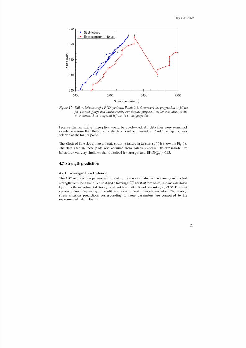
Figure 18: Ultimate strain-to-failure for RTD and ETW OHT specimens
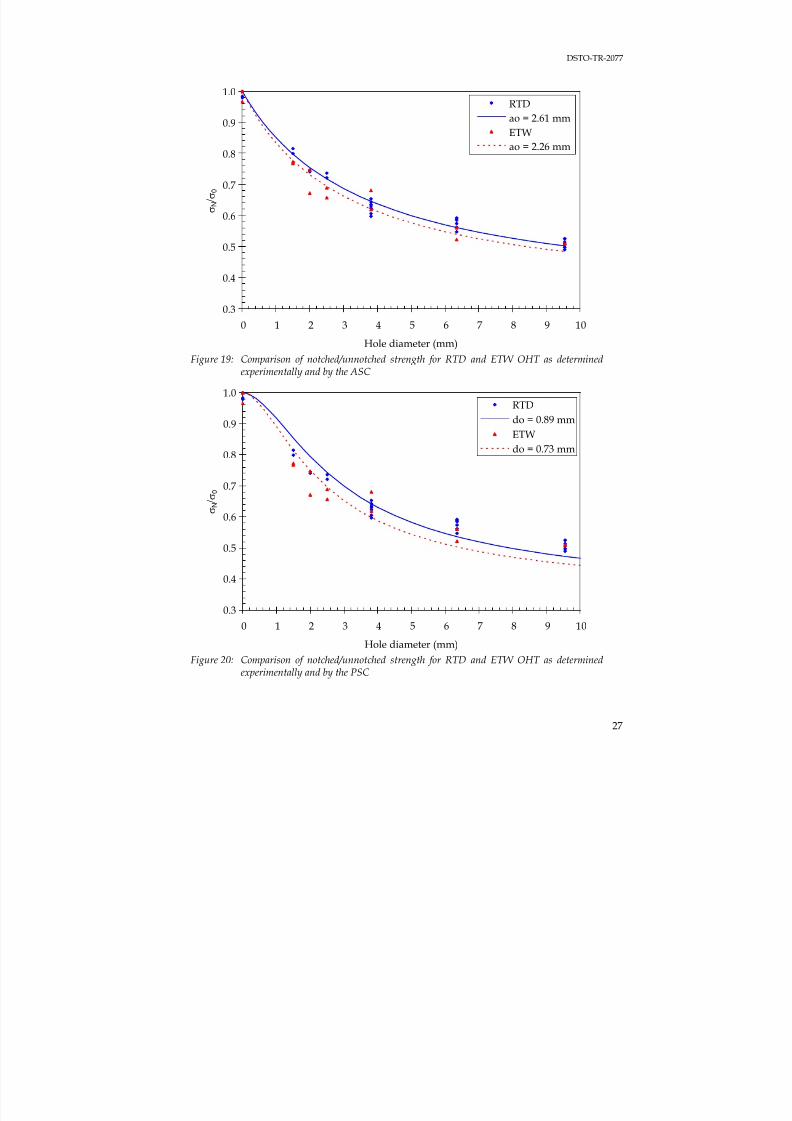
RTDσ
0 = 646 MPa a0 = 2.61 mm R2
= 0.986ETW σ0 = 632 MPa a0 = 2.26 mm R2 = 0.977
4.7.2 Point Stress Criterion
A similar approach was used to determine the PSC characteristic length, except that theexperimental strength data was fitted to Equation 6. The best fit curves are shown inFig. 20 and the calculated parameters are:
RTD σ0 = 646 MPa d0 = 0.89 mm R2 = 0.957
ETW σ0 = 632 MPa d0 = 0.73 mm R2 = 0.943
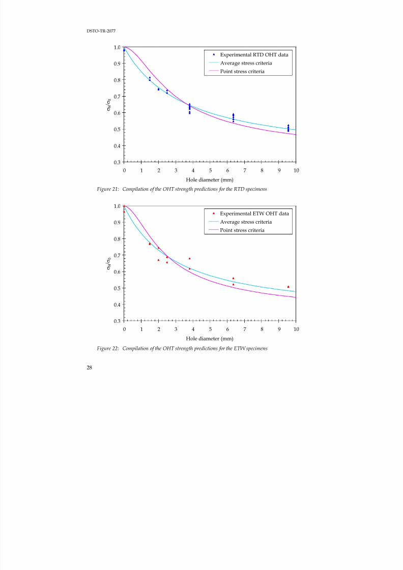
4.7.3 Compilation
The experimental data and average/point stress criteria predictions are plotted for theRTD specimens in Fig. 21 and the ETW specimens in Fig. 22.
The most appropriate method of comparing the fit of two equations, and thus choosingone model over another, is the F test [12], however performing this test was beyond thescope of this work. Instead it was noted that the coefficient of determination (R2) for boththe ASC and PSC were relatively high. Thus the predictions produced by both criteria
3000
4000
5000
6000
7000
8000
9000
10000
11000
1200013000
14000
15000
0 1 2 3 4 5 6 7 8 9 10
Hole diameter (mm)
S t r a i n ( m i c r o s t r a i n )
RTD
RTD average
ETWETW average
7/31/2019 Effect Hole Size Env Callus DSTO TR 2077
http://slidepdf.com/reader/full/effect-hole-size-env-callus-dsto-tr-2077 37/82
DSTO-TR-2077
27
Figure 19: Comparison of notched/unnotched strength for RTD and ETW OHT as determinedexperimentally and by the ASC
Figure 20: Comparison of notched/unnotched strength for RTD and ETW OHT as determinedexperimentally and by the PSC
0.3
0.4
0.5
0.6
0.7
0.8
0.9
1.0
0 1 2 3 4 5 6 7 8 9 10
Hole diameter (mm)
σ N
/ σ 0
RTD
do = 0.89 mm
ETW
do = 0.73 mm
0.3
0.4
0.5
0.6
0.7
0.8
0.9
1.0
0 1 2 3 4 5 6 7 8 9 10
Hole diameter (mm)
σ N
/ σ 0
RTD
ao = 2.61 mm
ETWao = 2.26 mm
7/31/2019 Effect Hole Size Env Callus DSTO TR 2077
http://slidepdf.com/reader/full/effect-hole-size-env-callus-dsto-tr-2077 38/82
DSTO-TR-2077
28
Figure 21: Compilation of the OHT strength predictions for the RTD specimens
Figure 22: Compilation of the OHT strength predictions for the ETW specimens
0.3
0.4
0.5
0.6
0.7
0.8
0.9
1.0
0 1 2 3 4 5 6 7 8 9 10
Hole diameter (mm)
σ N
/ σ 0
Experimental ETW OHT data
Average stress criteria
Point stress criteria
0.3
0.4
0.5
0.6
0.7
0.8
0.9
1.0
0 1 2 3 4 5 6 7 8 9 10
Hole diameter (mm)
σ N
/ σ 0
Experimental RTD OHT data
Average stress criteria
Point stress criteria
7/31/2019 Effect Hole Size Env Callus DSTO TR 2077
http://slidepdf.com/reader/full/effect-hole-size-env-callus-dsto-tr-2077 39/82
DSTO-TR-2077
29
were good. Figures 21 and 22 show that, visually, the shape of the ASC curve appeared tomatch the experimental data more closely than the PSC for both the RTD and ETWconditions.
The improved match of the ASC was also observed in [1] and attributed to the ASC
considering a larger volume of material than the PSC (a0 ≈ 2.8 d0). It was argued thattensile failure in composites is governed by the interaction between flaws (misalignedfibres, disbonded fibres, porosity, matrix yielding) and the local stress field. Thedistribution of flaws is statistical, therefore those criteria that consider greater volumes ofmaterial increase the likelihood of including the critical flaws that precipitate specimenfailure. It is possible that the length a0 is required to fully enclose the flaws that lead tofailure within a notched composite while the distance d0 is insufficient. Detailedmicrostructural studies would be required to test this hypothesis, however such work wasbeyond the scope of this program.
4.8 Length scales
The analytical solutions to the ASC and PSC were shown in Section 4.7. The length scalesas determined using two other methods were also determined and are shown here forcomparison.
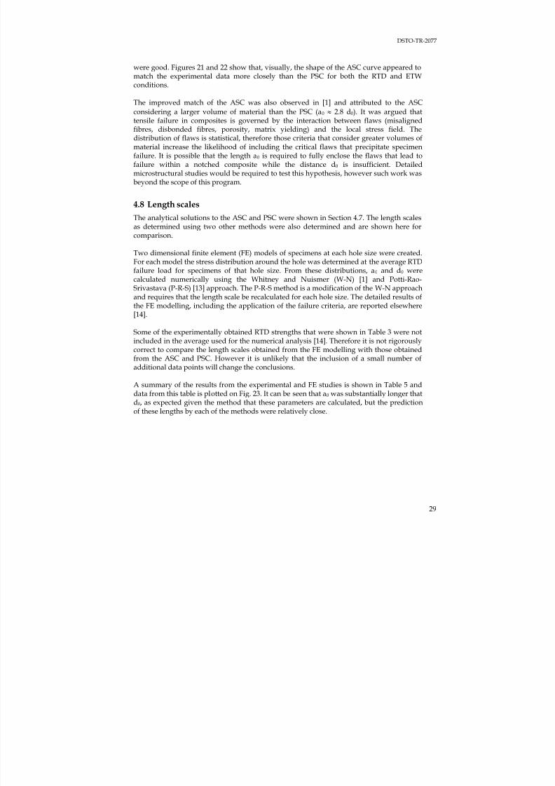
Two dimensional finite element (FE) models of specimens at each hole size were created.For each model the stress distribution around the hole was determined at the average RTDfailure load for specimens of that hole size. From these distributions, a0 and d0 werecalculated numerically using the Whitney and Nuismer (W-N) [1] and Potti-Rao-
Srivastava (P-R-S) [13] approach. The P-R-S method is a modification of the W-N approachand requires that the length scale be recalculated for each hole size. The detailed results ofthe FE modelling, including the application of the failure criteria, are reported elsewhere[14].
Some of the experimentally obtained RTD strengths that were shown in Table 3 were notincluded in the average used for the numerical analysis [14]. Therefore it is not rigorouslycorrect to compare the length scales obtained from the FE modelling with those obtainedfrom the ASC and PSC. However it is unlikely that the inclusion of a small number ofadditional data points will change the conclusions.
A summary of the results from the experimental and FE studies is shown in Table 5 anddata from this table is plotted on Fig. 23. It can be seen that a0 was substantially longer thatd0, as expected given the method that these parameters are calculated, but the predictionof these lengths by each of the methods were relatively close.
7/31/2019 Effect Hole Size Env Callus DSTO TR 2077
http://slidepdf.com/reader/full/effect-hole-size-env-callus-dsto-tr-2077 40/82
DSTO-TR-2077
30
Table 5: The ASC and PSC characteristic lengths for OHT as calculated using the Whitney-Nuismer (W-N) and Potti-Rao-Srivastava (P-R-S) approaches
ASC length scale a0 (mm) PSC length scale d0 (mm)
W-N W-NHole
diameter(mm) Analytical FE
P-R-S Analytical
FEP-R-S
1.50 2.20 2.49 1.07 0.66
2.00 2.29 2.53 1.08 0.73
2.50 2.64 2.56 1.16 0.78
3.81 2.17 2.63 1.01 0.89
6.35 2.65 2.71 1.29 1.02
9.55
2.61
2.55 2.76
0.89
1.14 1.12
Figure 23: Effect of hole size on critical length for RTD OHT models
0.0
0.5
1.0
1.5
2.0
2.5
3.0
0 1 2 3 4 5 6 7 8 9 10
Hole diameter (mm)
C h a r a c t e r i s t i c l e n g t h ( m m )
a0 (mm) W-N Analytical d0 (mm) W-N Analytical
a0 (mm) W-N FE d0 (mm) W-N FE
a0 (mm) P-R-S d0 (mm) P-R-S
7/31/2019 Effect Hole Size Env Callus DSTO TR 2077
http://slidepdf.com/reader/full/effect-hole-size-env-callus-dsto-tr-2077 41/82
DSTO-TR-2077
31
5 Results and Discussion - Compression
5.1 Stress-strain behaviour
5.1.1 Strain gauge
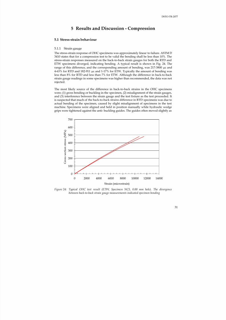
The stress-strain response of OHC specimens was approximately linear to failure. ASTM D3410 states that for a compression test to be valid the bending shall be less than 10%. Thestress-strain responses measured on the back-to-back strain gauges for both the RTD andETW specimens diverged, indicating bending. A typical result is shown in Fig. 24. The
range of this difference, and the corresponding amount of bending, was 217-3800 με and
4-63% for RTD and 182-911 με and 1-17% for ETW. Typically the amount of bending wasless than 8% for RTD and less than 7% for ETW. Although the difference in back-to-back
strain gauge readings in some specimens was higher than recommended, the data was notrejected.
The most likely source of the difference in back-to-back strains in the OHC specimenswere; (1) gross bending or buckling in the specimen, (2) misalignment of the strain gauges,and (3) interference between the strain gauge and the test fixture as the test proceeded. Itis suspected that much of the back-to-back strains difference in RTD specimens was due toactual bending of the specimen, caused by slight misalignment of specimens in the testmachine. Specimens were aligned and held in position manually while hydraulic wedgegrips were tightened against the anti- buckling guides. The guides often moved slightly as
Figure 24: Typical OHC test result (ETW, Specimen NC5, 0.00 mm hole). The divergencebetween back-to-back strain gauge measurements indicated specimen bending
0
100
200
300
400
500
600
700
0 2000 4000 6000 8000 10000 12000 14000
Strain (microstrain)
G r o s s s e c t i o n s t r e s s ( M P a )

7/31/2019 Effect Hole Size Env Callus DSTO TR 2077
http://slidepdf.com/reader/full/effect-hole-size-env-callus-dsto-tr-2077 42/82
DSTO-TR-2077
32
the grips tightened. Although the gripping process was repeated if movement wasobserved it was not always possible to eliminate all movement. In future work physicallimits will be installed in test machines to prevent specimens from moving during the
gripping process.
In support of this conclusion was the observation that the ETW specimens were loaded byclamping the anti-buckling guides to compression platens using rigid, well aligned,mounts. The resultant differences in back-to-back strain readings were much lower thanfor the RTD specimens.
It is unlikely that the divergence in measured strains was due to gauge misalignment.Post-test examination of nineteen gauges on the RTD specimens showed that the gaugelocation varied from the nominal location by 1 to 2 mm and the misalignment anglebetween the gauge and the specimen varied from 0.1 to 0.7°. Such small angles would
have very little effect on the measured strains.
5.1.2 Extensometer
An extensometer was installed on the edge of some OHC specimens (see Fig. 6). Figure 25shows typical stress-strain responses for the extensometer and strain gauge for RTD andETW specimens. Severe slippage of the extensometer was noted on seven out of eight RTDspecimens, as indicated by the horizontal steps in the curve. Prior to slippage the strains
Figure 25: Comparison between and extensometer and strain gauge showing extensometer slippage for RTD (2.00 mm hole, specimen KB2) and excessive extensometer strain for ETW (6.35 mm hole, specimen JA5)
0
100
200
300
400
500
0 2000 4000 6000 8000 10000
Strain (microstrain)
S t r e s s ( M P a )
RTD strain gauge
RTD extensometer
ETW strain gauge
ETW extensometer
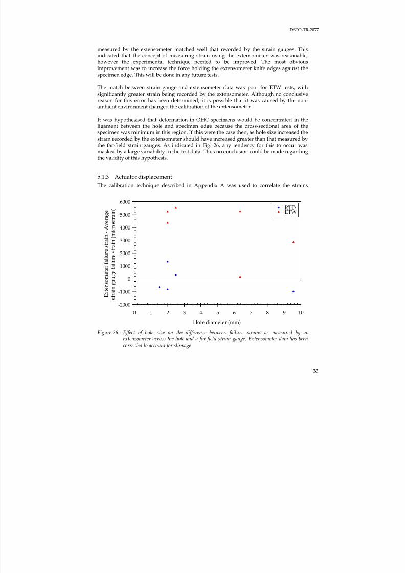
7/31/2019 Effect Hole Size Env Callus DSTO TR 2077
http://slidepdf.com/reader/full/effect-hole-size-env-callus-dsto-tr-2077 43/82
DSTO-TR-2077
33
measured by the extensometer matched well that recorded by the strain gauges. Thisindicated that the concept of measuring strain using the extensometer was reasonable,however the experimental technique needed to be improved. The most obvious
improvement was to increase the force holding the extensometer knife edges against thespecimen edge. This will be done in any future tests.
The match between strain gauge and extensometer data was poor for ETW tests, withsignificantly greater strain being recorded by the extensometer. Although no conclusivereason for this error has been determined, it is possible that it was caused by the non-ambient environment changed the calibration of the extensometer.
It was hypothesised that deformation in OHC specimens would be concentrated in theligament between the hole and specimen edge because the cross-sectional area of thespecimen was minimum in this region. If this were the case then, as hole size increased the
strain recorded by the extensometer should have increased greater than that measured bythe far-field strain gauges. As indicated in Fig. 26, any tendency for this to occur wasmasked by a large variability in the test data. Thus no conclusion could be made regardingthe validity of this hypothesis.
5.1.3 Actuator displacement
The calibration technique described in Appendix A was used to correlate the strains
Figure 26: Effect of hole size on the difference between failure strains as measured by anextensometer across the hole and a far field strain gauge. Extensometer data has beencorrected to account for slippage
-2000
-1000
0
1000
2000
3000
4000
5000
6000
0 1 2 3 4 5 6 7 8 9 10
Hole diameter (mm)
E x t e n s
o m e t e r f a i l u r e s t r a i n - A v e r a g e
s t r a i n g a u g e f a i l u r e s t r a i n ( m i c r o s t r a i n
) RTD
ETW
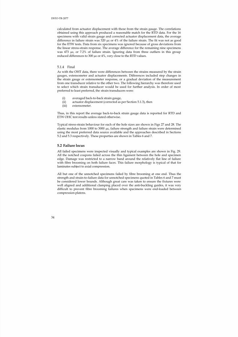
7/31/2019 Effect Hole Size Env Callus DSTO TR 2077
http://slidepdf.com/reader/full/effect-hole-size-env-callus-dsto-tr-2077 44/82
DSTO-TR-2077
34
calculated from actuator displacement with those from the strain gauge. The correlationsobtained using this approach produced a reasonable match for the RTD data. For the 16specimens with valid strain gauge and corrected actuator displacement data, the average
difference in failure strain was 320 με or 4% of the failure strain. The fit was not as goodfor the ETW tests. Data from six specimens was ignored because of gross deviations fromthe linear stress-strain response. The average difference for the remaining nine specimens
was 473 με, or 7.2% of failure strain. Ignoring data from three outliers in this group
reduced differences to 300 με or 4%, very close to the RTD values.
5.1.4 Final
As with the OHT data, there were differences between the strains measured by the straingauges, extensometer and actuator displacements. Differences included step changes inthe strain gauge or extensometer response, or a gradual deviation of the measurement
from one transducer relative to the other two. The following hierarchy was therefore usedto select which strain transducer would be used for further analysis. In order of mostpreferred to least preferred, the strain transducers were:
(i) averaged back-to-back strain gauge,(ii) actuator displacement (corrected as per Section 5.1.3), then(iii) extensometer.
Thus, in this report the average back-to-back strain gauge data is reported for RTD andETW OHC test results unless stated otherwise.
Typical stress-strain behaviour for each of the hole sizes are shown in Figs 27 and 28. Theelastic modulus from 1000 to 3000 με, failure strength and failure strain were determinedusing the most preferred data source available and the approaches described in Sections5.2 and 5.3 respectively. These properties are shown in Tables 6 and 7.
5.2 Failure locus
All failed specimens were inspected visually and typical examples are shown in Fig. 29.All the notched coupons failed across the thin ligament between the hole and specimenedge. Damage was restricted to a narrow band around the relatively flat line of failurewith fibre brooming on both failure faces. This failure morphology is typical of that for
laminates subject to axial compression.
All but one of the unnotched specimens failed by fibre brooming at one end. Thus thestrength and strain-to-failure data for unnotched specimens quoted in Tables 6 and 7 mustbe considered lower bounds. Although great care was taken to ensure the fixtures werewell aligned and additional clamping placed over the anti-buckling guides, it was verydifficult to prevent fibre brooming failures when specimens were end-loaded betweencompression platens.

7/31/2019 Effect Hole Size Env Callus DSTO TR 2077
http://slidepdf.com/reader/full/effect-hole-size-env-callus-dsto-tr-2077 45/82
DSTO-TR-2077
35
Figure 27: Typical stress-strain response of RTD OHC specimens with the indicated hole size
Figure 28: Typical stress-strain response of ETW OHC specimens with the indicated hole size
0
100
200
300
400
500
600
700
0 2000 4000 6000 8000 10000 12000 14000
Strain (microstrain)
S t r e s s ( M P a )
1.50 mm
2.50 mm
3.81 mm
6.35 mm
9.55 mm
0.00 mm
2.00 mm
0
100
200
300
400
500
600
700
0 2000 4000 6000 8000 10000 12000 14000
Strain (microstrain)
S t r e s s ( M P a ) 1.50 mm
2.50 mm
3.81 mm
6.35 mm
9.55 mm
0.00 mm
2.00 mm
7/31/2019 Effect Hole Size Env Callus DSTO TR 2077
http://slidepdf.com/reader/full/effect-hole-size-env-callus-dsto-tr-2077 46/82
DSTO-TR-2077
36
Table 6: RTD OHC results and derived mechanical data
Hole φ (mm)
Specimennumber
Thick.(mm)
Width(mm)
Pmax (kN)
c1E
(GPa) 1 cu1ε (με)1
cu1F
(MPa)FWCF
∞σN
(MPa)
33P3_1A 2.25 38.02 53.8 48.3 14,598 629 62933P3_12 2.34 38.09 51.8 47.5 13,443 583 58333P3_18 2.24 37.94 52.5 56.5 11,681 618 618
0.00
33P3_19 2.22 37.96 52.7 50.2 14,009 625
1.0000
625
KB5 2.24 38.14 39.8 46.6 10,981 466 1.0016 4671.50
KC3 2.31 38.17 38.5 47.8 9,785 437 1.0016 438
KA6 2.32 38.14 33.3 45.8 8,950 377 1.0029 3782.00
KB2 2.24 38.02 35.3 49.5 8,940 414 1.0029 415
KB3 2.31 38.11 34.9 45.0 9,222 397 1.0045 3992.50
KB4 2.25 38.14 31.4 49.0 7,554 366 1.0045 368
33P3_4 2.27 37.09 30.4 52.1 7,175 354 1.0114 35833P3_5 2.27 37.93 30.5 57.9 6,324 355 1.0108 35933P3_6 2.28 37.92 31.4 59.8 6,143 363 1.0108 367
3.81
KA3 2.25 38.02 29.8 53.1 6,602 348 1.0108 352
33P3_1 2.29 37.95 26.9 48.0 5,284 311 1.0317 32133P3_9 2.28 37.99 25.6 49.6 6,260 296 1.0317 305
33P3_10 2.29 37.95 27.5 54.3 6,272 318 1.0317 3286.35
KA4 2.27 38.12 25.1 53.2 - 290 1.0314 299
33P3_15 2.29 38.02 23.6 52.1 5,142 271 1.0772 29233P3_16 2.27 37.95 22.3 55.3 4,737 260 1.0775 28033P3_17 2.26 37.86 22.3 59.9 4,511 261 1.0779 281
9.55
KA5 2.29 38.05 24.3 50.8 5,850 279 1.0771 3011 The strain data source for modulus and failure strain is indicated by the colour of the
cell, being strain gauge or actuator displacement.
5.3 Modulus
The effects of hole size on OHC elastic modulus ( c1E ) are shown in Fig. 30. As with the
OHT specimens, the applied compression load was supported primarily by the 0° fibresand total volume of these fibres was not affected significantly by the relatively small holes.
Thus c1E was expected to be unaffected by hole size. This was observed for the ETW case
but it appeared that the average c1E rose as hole size increased. This trend was probablyan artefact of the broad scatter of results and was not considered a real effect.
5.4 Strength
The effects of hole size on ultimate OHC strength ( cu1F ) is shown in Fig. 31.
Using the approach described in Section 4.5, it was calculated that FcuETWEKDF = 0.81. This
was consistent for all hole sizes is similar to that reported in the literature. The
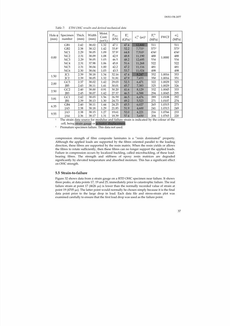
7/31/2019 Effect Hole Size Env Callus DSTO TR 2077
http://slidepdf.com/reader/full/effect-hole-size-env-callus-dsto-tr-2077 47/82
DSTO-TR-2077
37
Table 7: ETW OHC results and derived mechanical data
Hole φ
(mm)
Specimen
number
Thick.
(mm)
Width
(mm)
Moist.Cont.
(wt%)
Pmax
(kN)
c1E
(GPa) 1
cu1ε (με)1
cu1F
(MPa)
FWCF∞σN
(MPa)GB1 2.42 38.02 1.32 47.1 47.4 12,800 511 511GB2 2.38 38.12 1.42 33.82 52.2 7,7332 3732 3732 NC1 2.29 38.05 1.09 37.92 64.8 7,5102 4342 4342 NC2 2.31 38.09 1.08 42.9 48.8 11,190 488 488NC3 2.29 38.05 1.03 46.5 48.2 12,695 534 534NC4 2.31 37.98 1.06 45.8 51.6 11,268 522 522NC5 2.31 38.04 1.00 42.2 47.2 11,116 481 481
0.00
NC6 2.30 38.04 1.03 43.5 53.7 11,024 498
1.0000
498
JC1 2.39 38.18 1.34 32.16 47.4 8,247 352 1.0016 3531.50
JC2 2.39 38.05 1.32 31.81 47.9 7,653 350 1.0016 351
GC5 2.37 38.02 1.42 29.03 52.3 6,471 322 1.0029 3232.00
JB5 2.43 38.11 1.41 30.01 45.7 7,383 325 1.0029 326
GC2 2.40 38.00 0.91 30.20 41.6 8,129 332 1.0045 3332.50
JB3 2.45 38.07 1.42 27.37 46.5 6,588 294 1.0045 295
GC1 2.42 38.03 1.56 26.59 46.5 6,476 289 1.0108 2923.81
JB1 2.39 38.13 1.30 24.73 49.2 5,523 271 1.0107 274
GB4 2.40 38.11 1.44 24.25 45.5 6,027 265 1.0315 2736.35
JA5 2.38 38.18 1.29 21.85 51.9 4,600 241 1.0313 249
JA3 2.38 38.15 1.27 19.61 52.0 4,221 216 1.0766 2339.55
JA4 2.36 38.17 1.31 18.39 57.4 3,650 204 1.0765 2201
The strain data source for modulus and failure strain is indicated by the colour of thecell, being strain gauge or actuator displacement.2 Premature specimen failure. This data not used.
compression strength of fibre composite laminates is a “resin dominated” property.Although the applied loads are supported by the fibres oriented parallel to the loadingdirection, these fibres are supported by the resin matrix. When the resin yields or allowsthe fibres to rotate sufficiently, then these fibres can no longer support the applied loads.Failure in compression occurs by localized buckling, called microbuckling, of these load-bearing fibres. The strength and stiffness of epoxy resin matrices are degraded
significantly by elevated temperature and absorbed moisture. This has a significant effecton OHC strength.
5.5 Strain-to-failure
Figure 32 shows data from a strain gauge on a RTD OHC specimen near failure. It showsthree peaks, at data points 17, 19 and 25, immediately prior to catastrophic failure. The real
failure strain at point 17 (4626 με) is lower than the normally recorded value of strain at
point 19 (4705 με). The latter point would normally be chosen simply because it is the finaldata point prior to the large drop in load. Each data file and stress-strain plot wasexamined carefully to ensure that the first load drop was used as the failure point.
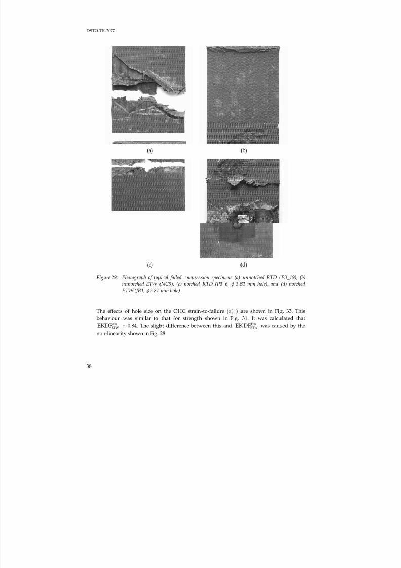
7/31/2019 Effect Hole Size Env Callus DSTO TR 2077
http://slidepdf.com/reader/full/effect-hole-size-env-callus-dsto-tr-2077 48/82
DSTO-TR-2077
38
(a) (b)
(c) (d)
Figure 29: Photograph of typical failed compression specimens (a) unnotched RTD (P3_19), (b)
unnotched ETW (NC5), (c) notched RTD (P3_6, φ 3.81 mm hole), and (d) notched
ETW (JB1, φ 3.81 mm hole)
The effects of hole size on the OHC strain-to-failure ( cu1ε ) are shown in Fig. 33. This
behaviour was similar to that for strength shown in Fig. 31. It was calculated thatcu
ETWEKDFε = 0.84. The slight difference between this and FcuETWEKDF was caused by the
non-linearity shown in Fig. 28.
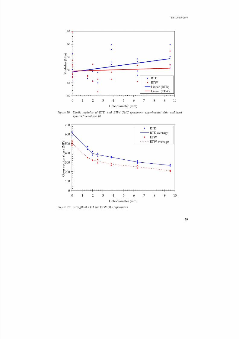
7/31/2019 Effect Hole Size Env Callus DSTO TR 2077
http://slidepdf.com/reader/full/effect-hole-size-env-callus-dsto-tr-2077 49/82
DSTO-TR-2077
39
Figure 30: Elastic modulus of RTD and ETW OHC specimens, experimental data and leastsquares lines of best fit
Figure 31: Strength of RTD and ETW OHC specimens
40
45
50
55
60
65
0 1 2 3 4 5 6 7 8 9 10
Hole diameter (mm)
M o d u l u s ( G P a )
RTD
ETWLinear (RTD)
Linear (ETW)
0
100
200
300
400
500
600
700
0 1 2 3 4 5 6 7 8 9 10
Hole diameter (mm)
G r o s s s e c t i o n s t r e s s ( M P a )
RTD
RTD average
ETW
ETW average

7/31/2019 Effect Hole Size Env Callus DSTO TR 2077
http://slidepdf.com/reader/full/effect-hole-size-env-callus-dsto-tr-2077 50/82
DSTO-TR-2077
40
Figure 32: Example of an RTD OHC coupon with a multi-step failure. The data point numbers areindicated (9.55 mm hole, specimen 33P3_16)
Figure 33: Failure strain for RTD and ETW OHC specimens
3000
4000
5000
6000
7000
8000
9000
10000
11000
12000
13000
14000
15000
0 1 2 3 4 5 6 7 8 9 10
Hole diameter (mm)
S
t r a i n ( m i c r o s t r a i n )
RTDRTD average
ETW
ETW average
230
240
250
260
270
4000 4100 4200 4300 4400 4500 4600 4700 4800
Strain (microstrain)
G r o s s s e c t i o n s t r e s s ( M P a )
1 2 3
4 5 6
78
9 1011
12 1314
15 16
17
1819
20
21
22
23
24 25
26
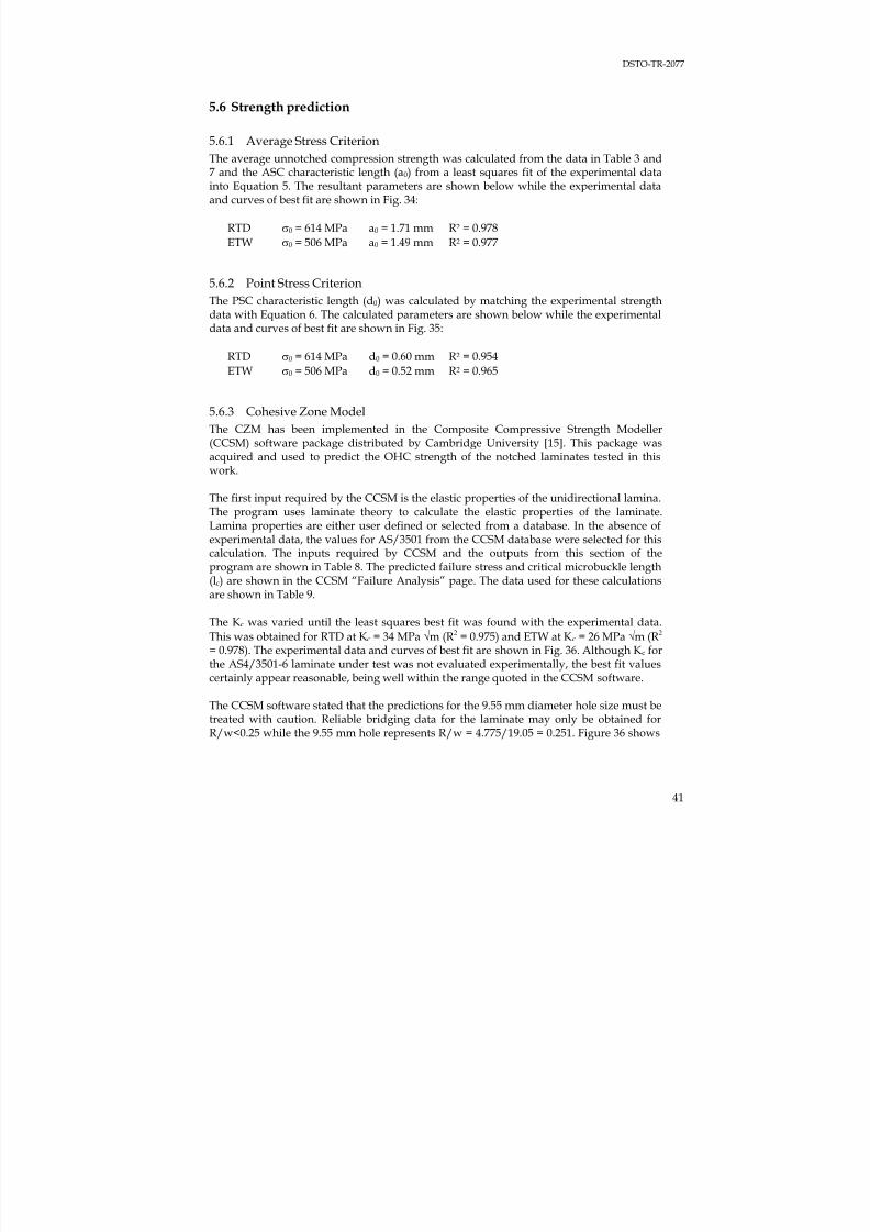
7/31/2019 Effect Hole Size Env Callus DSTO TR 2077
http://slidepdf.com/reader/full/effect-hole-size-env-callus-dsto-tr-2077 51/82
DSTO-TR-2077
41
5.6 Strength prediction
5.6.1 Average Stress Criterion
The average unnotched compression strength was calculated from the data in Table 3 and7 and the ASC characteristic length (a0) from a least squares fit of the experimental datainto Equation 5. The resultant parameters are shown below while the experimental dataand curves of best fit are shown in Fig. 34:
RTD σ0 = 614 MPa a0 = 1.71 mm R2 = 0.978
ETW σ0 = 506 MPa a0 = 1.49 mm R2 = 0.977
5.6.2 Point Stress Criterion
The PSC characteristic length (d0) was calculated by matching the experimental strengthdata with Equation 6. The calculated parameters are shown below while the experimentaldata and curves of best fit are shown in Fig. 35:
RTD σ0 = 614 MPa d0 = 0.60 mm R2 = 0.954
ETW σ0 = 506 MPa d0 = 0.52 mm R2 = 0.965
5.6.3 Cohesive Zone Model
The CZM has been implemented in the Composite Compressive Strength Modeller(CCSM) software package distributed by Cambridge University [15]. This package was
acquired and used to predict the OHC strength of the notched laminates tested in thiswork.
The first input required by the CCSM is the elastic properties of the unidirectional lamina.The program uses laminate theory to calculate the elastic properties of the laminate.Lamina properties are either user defined or selected from a database. In the absence ofexperimental data, the values for AS/3501 from the CCSM database were selected for thiscalculation. The inputs required by CCSM and the outputs from this section of theprogram are shown in Table 8. The predicted failure stress and critical microbuckle length(lc) are shown in the CCSM “Failure Analysis” page. The data used for these calculationsare shown in Table 9.
The Kc was varied until the least squares best fit was found with the experimental data.
This was obtained for RTD at Kc = 34 MPa √m (R2 = 0.975) and ETW at Kc = 26 MPa √m (R2 = 0.978). The experimental data and curves of best fit are shown in Fig. 36. Although Kc forthe AS4/3501-6 laminate under test was not evaluated experimentally, the best fit valuescertainly appear reasonable, being well within the range quoted in the CCSM software.
The CCSM software stated that the predictions for the 9.55 mm diameter hole size must betreated with caution. Reliable bridging data for the laminate may only be obtained forR/w<0.25 while the 9.55 mm hole represents R/w = 4.775/19.05 = 0.251. Figure 36 shows
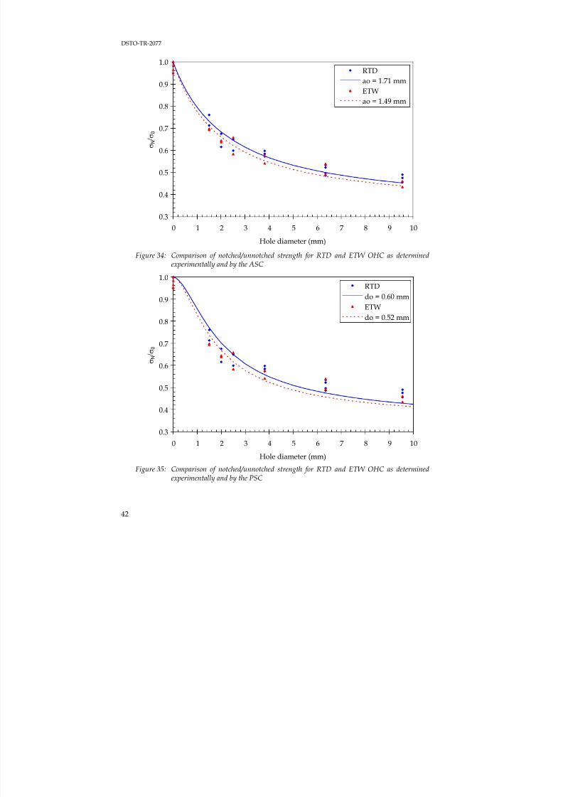
7/31/2019 Effect Hole Size Env Callus DSTO TR 2077
http://slidepdf.com/reader/full/effect-hole-size-env-callus-dsto-tr-2077 52/82
DSTO-TR-2077
42
Figure 34: Comparison of notched/unnotched strength for RTD and ETW OHC as determinedexperimentally and by the ASC
Figure 35: Comparison of notched/unnotched strength for RTD and ETW OHC as determinedexperimentally and by the PSC
0.3
0.4
0.5
0.6
0.7
0.8
0.9
1.0
0 1 2 3 4 5 6 7 8 9 10
Hole diameter (mm)
σ N
/ σ 0
RTD
do = 0.60 mmETW
do = 0.52 mm
0.3
0.4
0.5
0.6
0.7
0.8
0.9
1.0
0 1 2 3 4 5 6 7 8 9 10
Hole diameter (mm)
σ N
/ σ 0
RTD
ao = 1.71 mm
ETW
ao = 1.49 mm
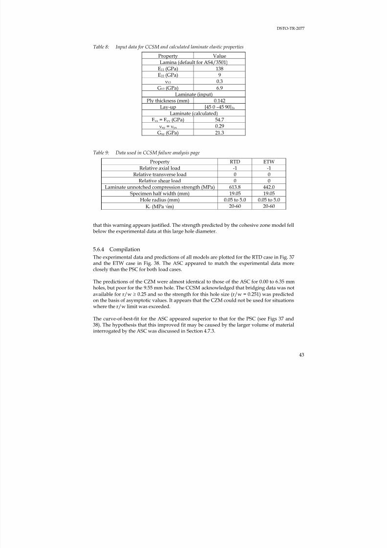
7/31/2019 Effect Hole Size Env Callus DSTO TR 2077
http://slidepdf.com/reader/full/effect-hole-size-env-callus-dsto-tr-2077 53/82
DSTO-TR-2077
43
Table 8: Input data for CCSM and calculated laminate elastic properties
Property ValueLamina (default for AS4/3501)
E11 (GPa) 138E22 (GPa) 9
ν12 0.3
G12 (GPa) 6.9Laminate (input)
Ply thickness (mm) 0.142Lay-up [45 0 –45 90]2s
Laminate (calculated)Exx = Eyy (GPa) 54.7
νxy = νyx 0.29
Gxy (GPa) 21.3
Table 9: Data used in CCSM failure analysis page
Property RTD ETWRelative axial load -1 -1
Relative transverse load 0 0Relative shear load 0 0
Laminate unnotched compression strength (MPa) 613.8 442.0Specimen half width (mm) 19.05 19.05
Hole radius (mm) 0.05 to 5.0 0.05 to 5.0
Kc (MPa √m) 20-60 20-60
that this warning appears justified. The strength predicted by the cohesive zone model fellbelow the experimental data at this large hole diameter.
5.6.4 Compilation
The experimental data and predictions of all models are plotted for the RTD case in Fig. 37and the ETW case in Fig. 38. The ASC appeared to match the experimental data more
closely than the PSC for both load cases.
The predictions of the CZM were almost identical to those of the ASC for 0.00 to 6.35 mmholes, but poor for the 9.55 mm hole. The CCSM acknowledged that bridging data was not
available for r/w ≥ 0.25 and so the strength for this hole size (r/w = 0.251) was predictedon the basis of asymptotic values. It appears that the CZM could not be used for situationswhere the r/w limit was exceeded.
The curve-of-best-fit for the ASC appeared superior to that for the PSC (see Figs 37 and38). The hypothesis that this improved fit may be caused by the larger volume of materialinterrogated by the ASC was discussed in Section 4.7.3.
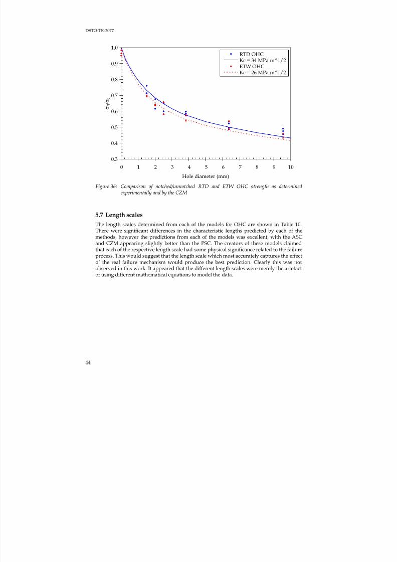
7/31/2019 Effect Hole Size Env Callus DSTO TR 2077
http://slidepdf.com/reader/full/effect-hole-size-env-callus-dsto-tr-2077 54/82
DSTO-TR-2077
44
Figure 36: Comparison of notched/unnotched RTD and ETW OHC strength as determinedexperimentally and by the CZM
5.7 Length scales
The length scales determined from each of the models for OHC are shown in Table 10. There were significant differences in the characteristic lengths predicted by each of themethods, however the predictions from each of the models was excellent, with the ASCand CZM appearing slightly better than the PSC. The creators of these models claimedthat each of the respective length scale had some physical significance related to the failureprocess. This would suggest that the length scale which most accurately captures the effectof the real failure mechanism would produce the best prediction. Clearly this was notobserved in this work. It appeared that the different length scales were merely the artefactof using different mathematical equations to model the data.
0.3
0.4
0.5
0.6
0.7
0.8
0.9
1.0
0 1 2 3 4 5 6 7 8 9 10
Hole diameter (mm)
σ N
/ σ 0
RTD OHCKc = 34 MPa m^1/2
ETW OHCKc = 26 MPa m^1/2
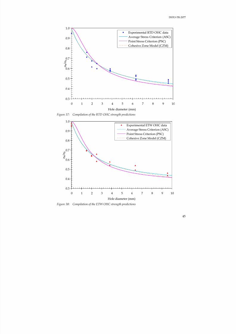
7/31/2019 Effect Hole Size Env Callus DSTO TR 2077
http://slidepdf.com/reader/full/effect-hole-size-env-callus-dsto-tr-2077 55/82
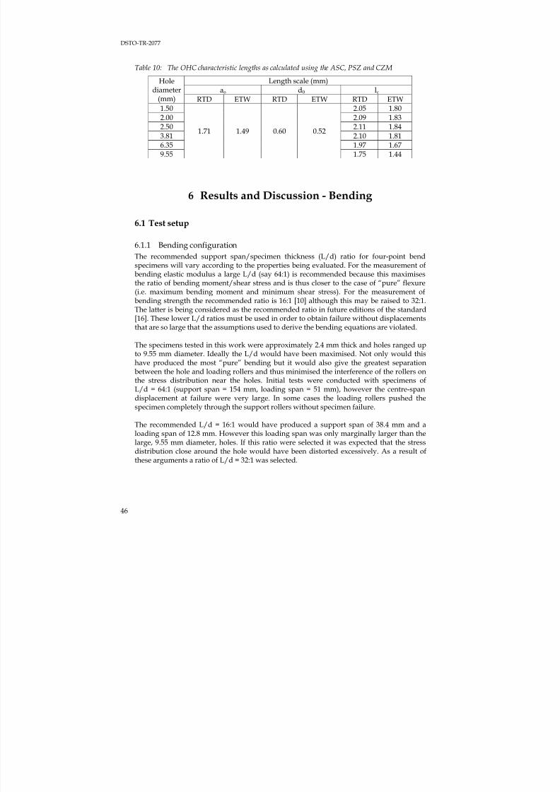
7/31/2019 Effect Hole Size Env Callus DSTO TR 2077
http://slidepdf.com/reader/full/effect-hole-size-env-callus-dsto-tr-2077 56/82
DSTO-TR-2077
46
Table 10: The OHC characteristic lengths as calculated using the ASC, PSZ and CZM
Length scale (mm)ao d0 lc
Holediameter
(mm) RTD ETW RTD ETW RTD ETW1.50 2.05 1.802.00 2.09 1.832.50 2.11 1.843.81 2.10 1.816.35 1.97 1.679.55
1.71 1.49 0.60 0.52
1.75 1.44
6 Results and Discussion - Bending
6.1 Test setup
6.1.1 Bending configuration
The recommended support span/specimen thickness (L/d) ratio for four-point bendspecimens will vary according to the properties being evaluated. For the measurement ofbending elastic modulus a large L/d (say 64:1) is recommended because this maximisesthe ratio of bending moment/shear stress and is thus closer to the case of “pure” flexure
(i.e. maximum bending moment and minimum shear stress). For the measurement ofbending strength the recommended ratio is 16:1 [10] although this may be raised to 32:1.The latter is being considered as the recommended ratio in future editions of the standard[16]. These lower L/d ratios must be used in order to obtain failure without displacementsthat are so large that the assumptions used to derive the bending equations are violated.
The specimens tested in this work were approximately 2.4 mm thick and holes ranged upto 9.55 mm diameter. Ideally the L/d would have been maximised. Not only would thishave produced the most “pure” bending but it would also give the greatest separationbetween the hole and loading rollers and thus minimised the interference of the rollers onthe stress distribution near the holes. Initial tests were conducted with specimens of
L/d = 64:1 (support span = 154 mm, loading span = 51 mm), however the centre-spandisplacement at failure were very large. In some cases the loading rollers pushed thespecimen completely through the support rollers without specimen failure.
The recommended L/d = 16:1 would have produced a support span of 38.4 mm and aloading span of 12.8 mm. However this loading span was only marginally larger than thelarge, 9.55 mm diameter, holes. If this ratio were selected it was expected that the stressdistribution close around the hole would have been distorted excessively. As a result ofthese arguments a ratio of L/d = 32:1 was selected.
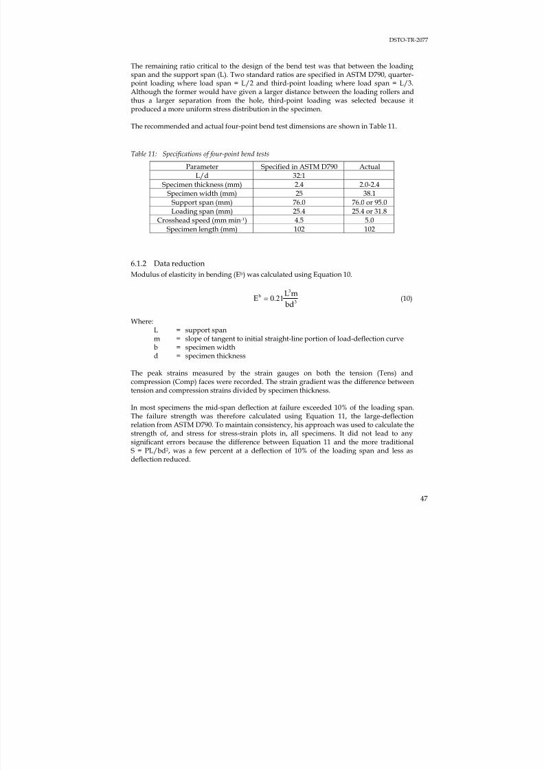
7/31/2019 Effect Hole Size Env Callus DSTO TR 2077
http://slidepdf.com/reader/full/effect-hole-size-env-callus-dsto-tr-2077 57/82
DSTO-TR-2077
47
The remaining ratio critical to the design of the bend test was that between the loadingspan and the support span (L). Two standard ratios are specified in ASTM D790, quarter-point loading where load span = L/2 and third-point loading where load span = L/3.
Although the former would have given a larger distance between the loading rollers andthus a larger separation from the hole, third-point loading was selected because itproduced a more uniform stress distribution in the specimen.
The recommended and actual four-point bend test dimensions are shown in Table 11.
Table 11: Specifications of four-point bend tests
Parameter Specified in ASTM D790 ActualL/d 32:1
Specimen thickness (mm) 2.4 2.0-2.4Specimen width (mm) 25 38.1
Support span (mm) 76.0 76.0 or 95.0Loading span (mm) 25.4 25.4 or 31.8
Crosshead speed (mm min-1) 4.5 5.0Specimen length (mm) 102 102
6.1.2 Data reduction
Modulus of elasticity in bending (Eb) was calculated using Equation 10.
3
3b
bd
mLE 21.0= (10)
Where:L = support spanm = slope of tangent to initial straight-line portion of load-deflection curveb = specimen widthd = specimen thickness
The peak strains measured by the strain gauges on both the tension (Tens) and
compression (Comp) faces were recorded. The strain gradient was the difference betweentension and compression strains divided by specimen thickness.
In most specimens the mid-span deflection at failure exceeded 10% of the loading span.The failure strength was therefore calculated using Equation 11, the large-deflectionrelation from ASTM D790. To maintain consistency, his approach was used to calculate thestrength of, and stress for stress-strain plots in, all specimens. It did not lead to anysignificant errors because the difference between Equation 11 and the more traditionalS = PL/bd2, was a few percent at a deflection of 10% of the loading span and less asdeflection reduced.
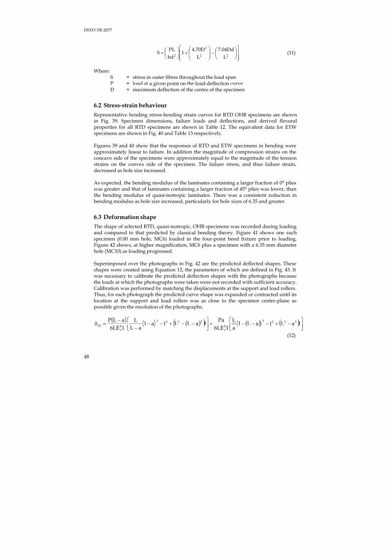
7/31/2019 Effect Hole Size Env Callus DSTO TR 2077
http://slidepdf.com/reader/full/effect-hole-size-env-callus-dsto-tr-2077 58/82
DSTO-TR-2077
48
⎥⎥⎦
⎤
⎢⎢⎣
⎡⎟ ⎠
⎞⎜⎝
⎛ −⎟⎟
⎠
⎞⎜⎜⎝
⎛ +⎟
⎠
⎞⎜⎝
⎛ =
22
2
2 L
7.04Dd
L
4.70D1
bd
PLS (11)
Where:S = stress in outer fibres throughout the load spanP = load at a given point on the load-deflection curveD = maximum deflection of the centre of the specimen
6.2 Stress-strain behaviour
Representative bending stress-bending strain curves for RTD OHB specimens are shownin Fig. 39. Specimen dimensions, failure loads and deflections, and derived flexuralproperties for all RTD specimens are shown in Table 12. The equivalent data for ETWspecimens are shown in Fig. 40 and Table 13 respectively.
Figures 39 and 40 show that the responses of RTD and ETW specimens in bending wereapproximately linear to failure. In addition the magnitude of compression strains on theconcave side of the specimens were approximately equal to the magnitude of the tensionstrains on the convex side of the specimen. The failure stress, and thus failure strain,decreased as hole size increased.
As expected, the bending modulus of the laminates containing a larger fraction of 0° plieswas greater and that of laminates containing a larger fraction of 45° plies was lower, thanthe bending modulus of quasi-isotropic laminates. There was a consistent reduction inbending modulus as hole size increased, particularly for hole sizes of 6.35 and greater.
6.3 Deformation shape
The shape of selected RTD, quasi-isotropic, OHB specimens was recorded during loadingand compared to that predicted by classical bending theory. Figure 41 shows one suchspecimen (0.00 mm hole, MC6) loaded in the four-point bend fixture prior to loading.Figure 42 shows, at higher magnification, MC6 plus a specimen with a 6.35 mm diameterhole (MC10) as loading progressed.
Superimposed over the photographs in Fig. 42 are the predicted deflected shapes. Theseshapes were created using Equation 12, the parameters of which are defined in Fig. 43. Itwas necessary to calibrate the predicted deflection shapes with the photographs becausethe loads at which the photographs were taken were not recorded with sufficient accuracy.Calibration was performed by matching the displacements at the support and load rollers.Thus, for each photograph the predicted curve shape was expanded or contracted until itslocation at the support and load rollers was as close to the specimen centre-plane aspossible given the resolution of the photographs.
( )
( )( )( ) ( ) ( ) ⎥⎦
⎤⎢⎣
⎡ −+−−−+⎥⎦
⎤⎢⎣
⎡ −−+−−−
−=δ laLaLl
a
L
I6LE
PalaLLal
aL
L
I6LE
aLP 2233
b1
2233
b1
l ll
(12)
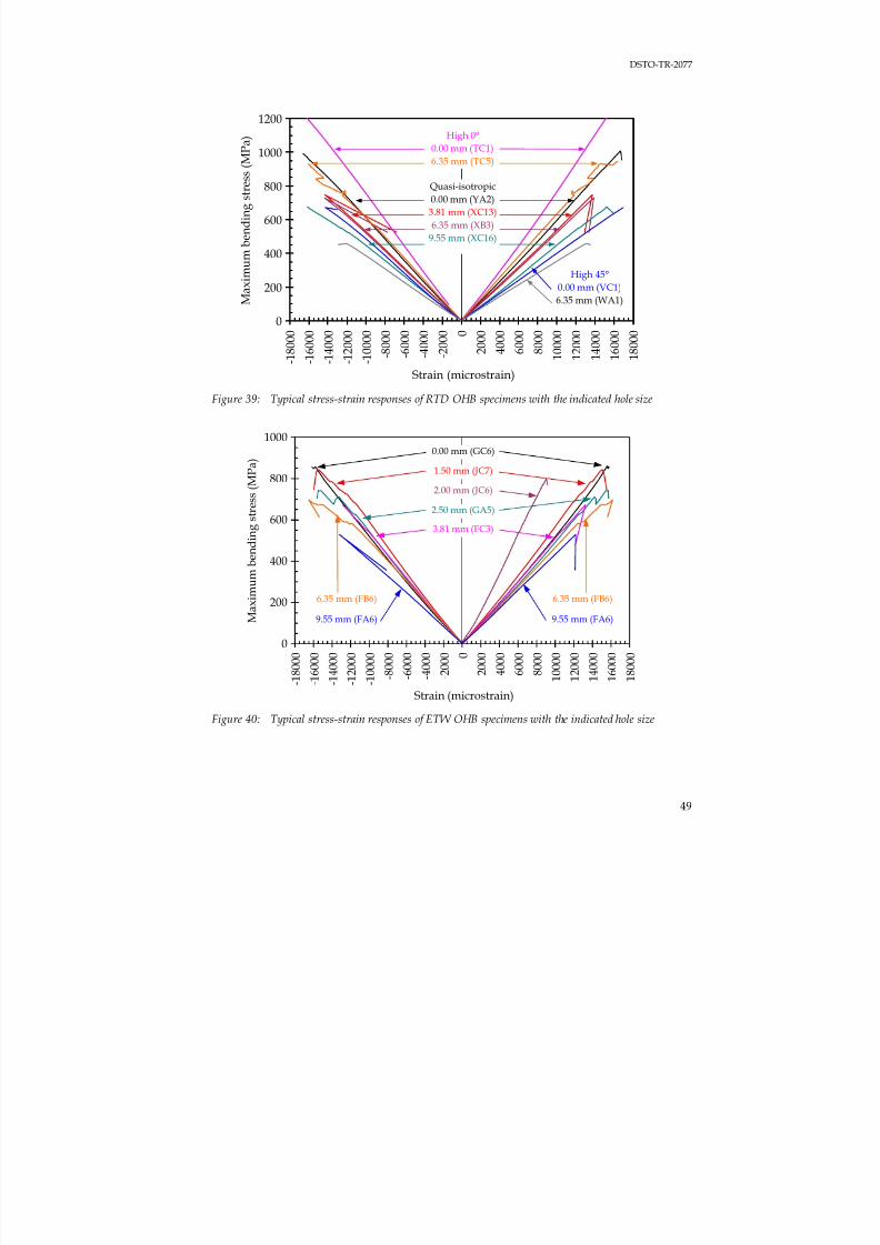
7/31/2019 Effect Hole Size Env Callus DSTO TR 2077
http://slidepdf.com/reader/full/effect-hole-size-env-callus-dsto-tr-2077 59/82
DSTO-TR-2077
49
Figure 39: Typical stress-strain responses of RTD OHB specimens with the indicated hole size
Figure 40: Typical stress-strain responses of ETW OHB specimens with the indicated hole size
0
200
400
600
800
1000
1200
- 1 8 0 0 0
- 1 6 0 0 0
- 1 4 0 0 0
- 1 2 0 0 0
- 1 0 0 0 0
- 8 0 0 0
- 6 0 0 0
- 4 0 0 0
- 2 0 0 0 0
2 0 0 0
4 0 0 0
6 0 0 0
8 0 0 0
1 0 0 0 0
1 2 0 0 0
1 4 0 0 0
1 6 0 0 0
1 8 0 0 0
Strain (microstrain)
M a x
i m u m
b e n
d i n g s t r e s s
( M P a
)
Quasi-isotropic
0.00 mm (YA2)
3.81 mm (XC13)
6.35 mm (XB3)
9.55 mm (XC16)
High 0°
0.00 mm (TC1)6.35 mm (TC5)
High 45°
0.00 mm (VC1)
6.35 mm (WA1)
0
200
400
600
800
1000
- 1 8 0 0 0
- 1 6 0 0 0
- 1 4 0 0 0
- 1 2 0 0 0
- 1 0 0 0 0
- 8 0 0 0
- 6 0 0 0
- 4 0 0 0
- 2 0 0 0 0
2 0 0 0
4 0 0 0
6 0 0 0
8 0 0 0
1 0 0 0 0
1 2 0 0 0
1 4 0 0 0
1 6 0 0 0
1 8 0 0 0
Strain (microstrain)
M
a x i m u m b e n d i n g s t r e s s ( M P a )
0.00 mm (GC6)
1.50 mm (JC7)
2.00 mm (JC6)
2.50 mm (GA5)
3.81 mm (FC3)
6.35 mm (FB6)
9.55 mm (FA6)
6.35 mm (FB6)
9.55 mm (FA6)
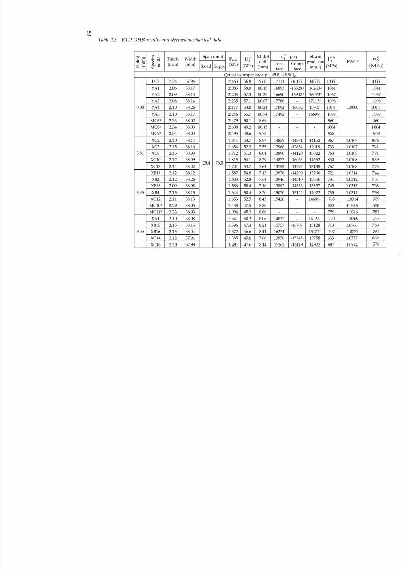
7/31/2019 Effect Hole Size Env Callus DSTO TR 2077
http://slidepdf.com/reader/full/effect-hole-size-env-callus-dsto-tr-2077 60/82
5 0
Table 12: RTD OHB results and derived mechanical data
Span (mm) bu1ε (με)
H o l e φ
( m m )
S p e c i m
e n I D Thick.
(mm)Width(mm) Load Supp.
Pmax (kN)
b1E
(GPa)
Midptdefl.(mm)
Tens.
face
Comp.
face
Strain
grad. (με mm-1)
bu1F
(MPa)
Quasi-isotropic lay-up - [45 0 –45 90]2s
LC2 2.24 37.94 2.463 56.8 9.68 17111 -16127 14855 1035
YA1 2.06 38.17 2.085 58.0 10.15 16893 -165282 162632 1041
YA2 2.09 38.13 2.205 57.3 10.35 16690 -169022 160732 1067
YA3 2.08 38.14 2.235 57.1 10.67 17786 - 171151 1098
YA4 2.10 38.26 2.117 53.0 10.24 17092 -16032 15807 1014
YA5 2.10 38.17 2.246 55.7 10.74 17492 - 166991 1087
MC63 2.33 38.02 2.479 50.1 8.69 - - - 960
MC83 2.34 38.03 2.600 49.2 10.15 - - - 1004
0.00
MC93 2.34 38.03 2.495 48.6 9.73 - - - 958
XC2 2.10 38.14 1.841 53.7 8.97 14859 -14861 14152 867 XC3 2.15 38.16 1.654 52.3 7.55 12968 -12854 12019 733
XC8 2.15 38.03 1.712 51.3 8.01 13890 -14120 13022 763
XC10 2.12 38.09 1.815 54.1 8.29 14877 -16053 14562 830
3.81
XC13 2.14 38.02 1.701 53.7 7.64 13752 -14297 13138 767
XB14 2.12 38.12 1.587 54.8 7.13 13878 -14290 13296 721
XB2 2.12 38.26 1.603 52.8 7.64 13946 -14310 13360 731
XB34 2.09 38.08 1.586 58.4 7.10 13892 -14333 13537 745
XB4 2.15 38.15 1.644 50.4 8.20 15070 -15122 14072 735
XC12 2.11 38.13 1.653 52.5 8.43 15426 - 146081 765
MC103 2.29 38.05 1.438 47.5 5.86 - - - 553
6.35
MC113 2.33 38.03 1.994 45.3 8.66 - - - 759
XA1 2.10 38.08 1.541 50.2 8.06 14832 - 141261 720
XB15 2.15 38.15 1.596 47.4 8.21 15757 -16707 15128 713
XB16 2.15 38.04 1.572 46.6 8.41 16274 - 151771 707
XC14 2.12 37.91 1.385 45.6 7.66 13976 -15245 13758 633
9.55
XC16 2.10 37.98
25.4 76.0
1.491 47.6 8.14 15262 -16119 14922 697
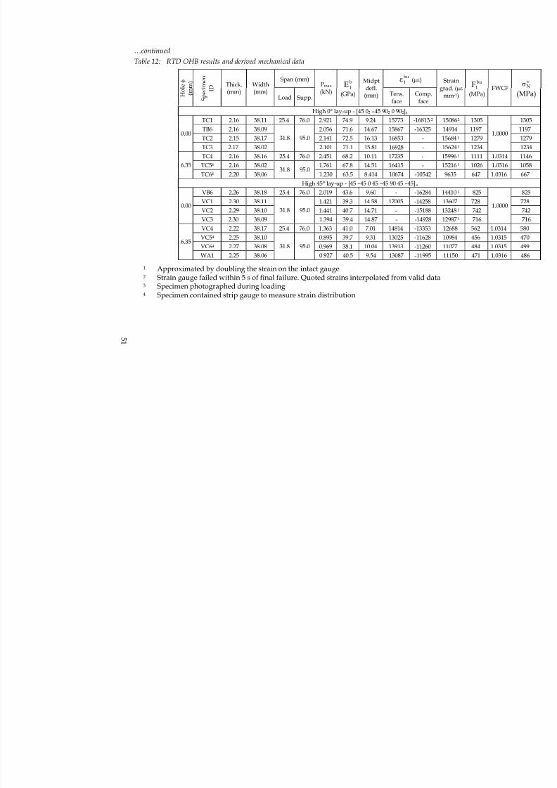
7/31/2019 Effect Hole Size Env Callus DSTO TR 2077
http://slidepdf.com/reader/full/effect-hole-size-env-callus-dsto-tr-2077 61/82
5 1
…continued
Table 12: RTD OHB results and derived mechanical data
Span (mm) bu1ε (με)
H o l e φ
( m m )
S p
e c i m e n
I DThick.(mm)
Width(mm)
Load Supp.
Pmax (kN)
b1E
(GPa)
Midptdefl.
(mm) Tens.face Comp.face
Strain
grad. (με
mm-1)
F
(M
High 0° lay-up - [45 02 –45 902 0 902]s
TC1 2.16 38.11 25.4 76.0 2.921 74.9 9.24 15773 -168132 150862 13
TB6 2.16 38.09 2.056 71.6 14.67 15867 -16325 14914 1
TC2 2.15 38.17 2.141 72.5 16.13 16853 - 156841 10.00
TC3 2.17 38.02
31.8 95.0
2.101 71.1 15.81 16928 - 156241 1
TC4 2.16 38.16 25.4 76.0 2.451 68.2 10.11 17235 - 159961 1
TC54 2.16 38.02 1.761 67.8 14.51 16415 - 152161 16.35
TC64 2.20 38.0631.8 95.0
1.230 63.5 8.414 10674 -10542 9635 6
High 45° lay-up - [45 –45 0 45 –45 90 45 –45]s
VB6 2.26 38.18 25.4 76.0 2.019 43.6 9.60 - -16284 144101 8VC1 2.30 38.11 1.421 39.3 14.58 17005 -14258 13607 7
VC2 2.29 38.10 1.441 40.7 14.71 - -15188 132481 70.00
VC3 2.30 38.09
31.8 95.0
1.394 39.4 14.87 - -14928 129871 7
VC4 2.22 38.17 25.4 76.0 1.363 41.0 7.01 14814 -13353 12688 5
VC54 2.25 38.10 0.895 39.7 9.31 13025 -11628 10984 4
VC64 2.27 38.08 0.969 38.1 10.04 13913 -11260 11077 46.35
WA1 2.25 38.06
31.8 95.0
0.927 40.5 9.54 13087 -11995 11150 4
1 Approximated by doubling the strain on the intact gauge2 Strain gauge failed within 5 s of final failure. Quoted strains interpolated from valid data3 Specimen photographed during loading4 Specimen contained strip gauge to measure strain distribution
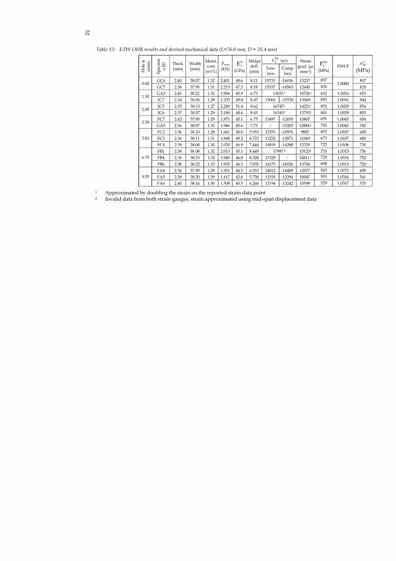
7/31/2019 Effect Hole Size Env Callus DSTO TR 2077
http://slidepdf.com/reader/full/effect-hole-size-env-callus-dsto-tr-2077 62/82
5 2
Table 13: ETW OHB results and derived mechanical data (L=76.0 mm, D = 25.4 mm)
bu1ε (με)
H o l e φ
( m
m )
S p e
c i m e
n
I DThick.
(mm)
Width
(mm)
Moist.cont.(wt%)
Pmax
(kN)
b1E
(GPa)
Midptdefl.(mm) Tens.
faceComp.
face
Strain
grad. (με mm-1)
bu1F
(MPa)
GC6 2.40 38.07 1.32 2.401 49.6 8.11 15733 -16036 13237 8570.00
GC7 2.36 37.95 1.31 2.213 47.3 8.18 15337 -14563 12640 820
GA3 2.43 38.22 1.32 1.904 45.9 6.73 130332 107261 652 1.50
JC7 2.34 38.06 1.28 2.235 49.8 8.47 15061 -15520 13069 843
JC5 2.35 38.13 1.27 2.280 51.6 8.62 167452 142511 852 2.00
JC6 2.37 38.07 1.29 2.180 48.6 8.41 163452 137931 801
FC7 2.42 37.95 1.29 1.871 45.1 6.75 13497 -12655 10807 6512.50
GA5 2.36 38.07 1.31 1.946 49.6 7.73 - -15203 128841 742
FC2 2.36 38.10 1.28 1.661 48.8 5.953 12353 -10976 9885 602
FC3 2.36 38.11 1.31 1.848 49.2 6.723 13252 -12871 11069 6733.81FC4 2.39 38.08 1.30 2.020 46.9 7.444 14818 -14388 12220 722
FB1 2.38 38.08 1.32 2.013 45.1 8.449 179972 151231 733
FB4 2.34 38.15 1.32 1.940 46.8 8.328 17329 - 148111 7296.35
FB6 2.38 38.22 1.33 1.935 46.3 7.876 16175 -16526 13740 698
FA4 2.36 37.99 1.29 1.551 44.5 6.353 14012 -14489 12077 565
FA5 2.38 38.20 1.29 1.417 42.8 5.758 11518 -12394 10047 5039.55
FA6 2.40 38.14 1.30 1.508 40.5 6.260 12194 -13242 10598 529
1 Approximated by doubling the strain on the reported strain data point2 Invalid data from both strain gauges, strain approximated using mid-span displacement data
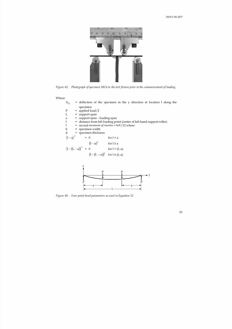
7/31/2019 Effect Hole Size Env Callus DSTO TR 2077
http://slidepdf.com/reader/full/effect-hole-size-env-callus-dsto-tr-2077 63/82
DSTO-TR-2077
53
Figure 41: Photograph of specimen MC6 in the test fixture prior to the commencement of loading
Where:
( )lδ = deflection of the specimen in the y direction at location l along the
specimenP = applied load/2L = support spana = support span – loading span
l = distance from left loading point (centre of left hand support roller)I = second moment of inertia = bd3/12 whereb = specimen widthd = specimen thickness
3al − = 0 for l < a
( )3al − for l ≥ a
( )3
aLl −− = 0 for l < (L-a)
( )( )3aLl −− for l ≥ (L-a)
Figure 43: Four point bend parameters as used in Equation 12
y
lP P
P Pa a
L
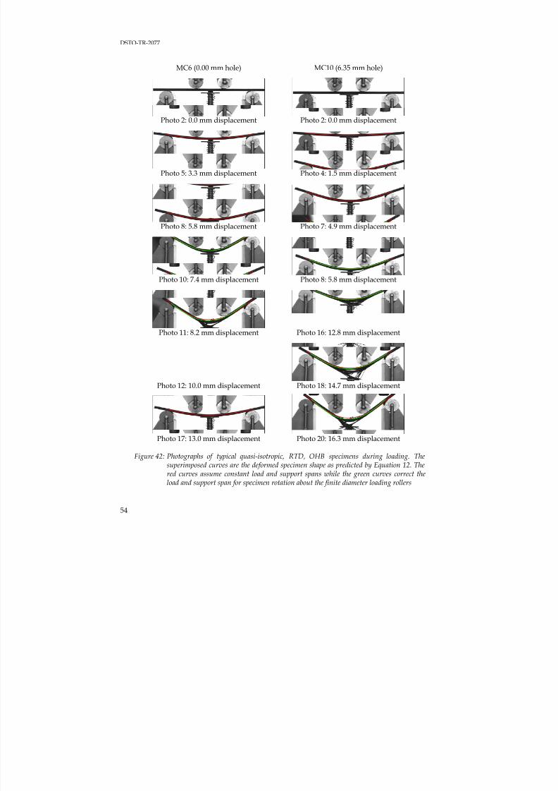
7/31/2019 Effect Hole Size Env Callus DSTO TR 2077
http://slidepdf.com/reader/full/effect-hole-size-env-callus-dsto-tr-2077 64/82
DSTO-TR-2077
54
MC6 (0.00 mm hole) MC10 (6.35 mm hole)
Photo 2: 0.0 mm displacement Photo 2: 0.0 mm displacement
Photo 5: 3.3 mm displacement Photo 4: 1.5 mm displacement
Photo 8: 5.8 mm displacement Photo 7: 4.9 mm displacement
Photo 10: 7.4 mm displacement Photo 8: 5.8 mm displacement
Photo 11: 8.2 mm displacement Photo 16: 12.8 mm displacement
Photo 12: 10.0 mm displacement Photo 18: 14.7 mm displacement
Photo 17: 13.0 mm displacement Photo 20: 16.3 mm displacement
Figure 42: Photographs of typical quasi-isotropic, RTD, OHB specimens during loading. Thesuperimposed curves are the deformed specimen shape as predicted by Equation 12. Thered curves assume constant load and support spans while the green curves correct theload and support span for specimen rotation about the finite diameter loading rollers
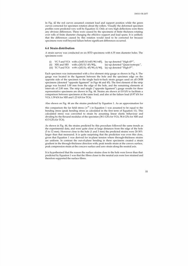
7/31/2019 Effect Hole Size Env Callus DSTO TR 2077
http://slidepdf.com/reader/full/effect-hole-size-env-callus-dsto-tr-2077 65/82
DSTO-TR-2077
55
In Fig. 42 the red curves assumed constant load and support position while the greencurves corrected for specimen rotation about the rollers. Visually the deformed specimenprofiles were predicted very well by Equation 12. Only at very high deflections were there
any obvious differences. These were caused by the specimens of finite thickness rotatingover rolls of finite diameter changing the effective support and load spans. It is unlikelythat the differences caused by this rotation would need to be corrected for becausespecimens were well beyond failure before significant differences occurred.
6.4 Strain distribution
A strain survey was conducted on six RTD specimens with 6.35 mm diameter holes. Thespecimens were:
(i) VC 5 and VC6 with a [±45/0/±45/90/±45]s lay-up denoted “High 45°”,
(ii) XB1 and XB3 with a [45/0/-45/90]2s lay-up denoted “Quasi-isotropic”,(iii) TC 5 and TC6 with a [45/02/-45/902/0/90]s lay-up denoted “High 0°”.
Each specimen was instrumented with a five element strip gauge as shown in Fig. 6. Thegauge was located in the ligament between the hole and the specimen edge on theopposite side of the specimen to the single back-to-back strain gauges used on all OHBspecimens (denoted “opposite ligament” in Figs 44 and 45). The first element of the stripgauge was located 1.00 mm from the edge of the hole, and the remaining elements atintervals of 2.00 mm. The strip and single (“opposite ligament”) gauge results for threerepresentative specimens are shown in Fig. 44. Strains are shown at 0.8 kN to facilitate acomparison between specimens at the same load, and also at the failure load (0.97 kN for
VC6, 1.59 kN for XB3 and 1.23 kN for TC6).
Also shown on Fig. 44 are the strains predicted by Equation 1. As an approximation for
this comparison the far field stress ( ∞σ ) in Equation 1 was assumed to be equal to thebending stress (peak bending stress as calculated in the first term of Equation 11). Thiscalculated stress was converted to strain by assuming linear elastic behaviour anddividing by the flexural modulus of the specimen (38.1 GPa for VC6, 58.4 GPa for XB3 and63.5 GPa for TC6).
As shown in Fig. 44, the strains predicted by this procedure followed the same trends asthe experimental data, and were quite close at large distances from the edge of the hole
(5 to 12 mm). However close to the hole (1 and 3 mm) the predicted strains were 20-30%larger than that measured. It is quite surprising that the prediction was even this close,given that Equation 1 was derived for in-plane tension where through-thickness strainsare uniform. In contrast the out-of-plane bending in these specimens created a straingradient in the through-thickness direction with; peak tensile strain at the convex surface,peak compression strain at the concave surface and zero strain along the neutral axis.
It is hypothesised that the reason the surface strains close to the hole were lower than thatpredicted by Equation 1 was that the fibres closer to the neutral axis were less strained andtherefore supported the surface fibres.
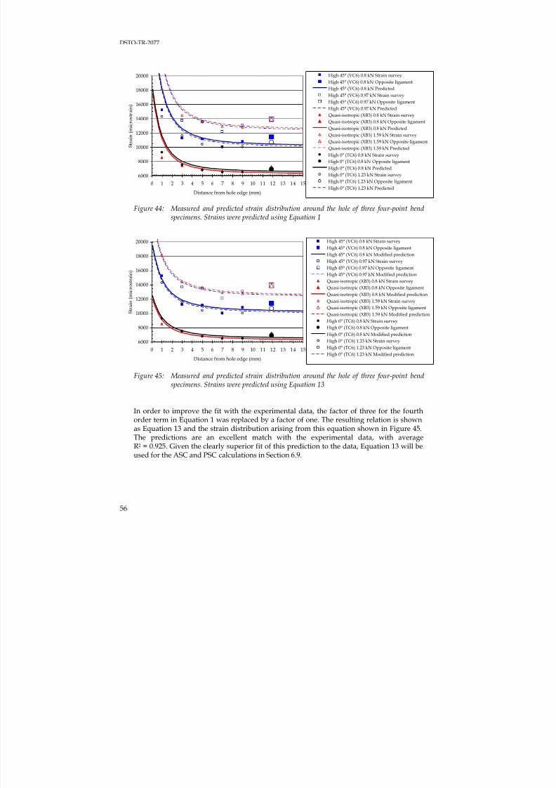
7/31/2019 Effect Hole Size Env Callus DSTO TR 2077
http://slidepdf.com/reader/full/effect-hole-size-env-callus-dsto-tr-2077 66/82
DSTO-TR-2077
56
Figure 44: Measured and predicted strain distribution around the hole of three four-point bendspecimens. Strains were predicted using Equation 1
Figure 45: Measured and predicted strain distribution around the hole of three four-point bendspecimens. Strains were predicted using Equation 13
In order to improve the fit with the experimental data, the factor of three for the fourthorder term in Equation 1 was replaced by a factor of one. The resulting relation is shownas Equation 13 and the strain distribution arising from this equation shown in Figure 45.The predictions are an excellent match with the experimental data, with averageR2 = 0.925. Given the clearly superior fit of this prediction to the data, Equation 13 will beused for the ASC and PSC calculations in Section 6.9.
6000
8000
10000
12000
14000
16000
18000
20000
0 1 2 3 4 5 6 7 8 9 10 11 12 13 14 15
Distance from hole edge (mm)
S t r a i n ( m i c r o s t r a
i n )
High 45° (VC6) 0.8 kN Strain survey
High 45° (VC6) 0.8 kN Opposite ligament
High 45° (VC6) 0.8 kN Predicted
High 45° (VC6) 0.97 kN Strain surveyHigh 45° (VC6) 0.97 kN Opposite ligament
High 45° (VC6) 0.97 kN Predicted
Quasi-isotropic (XB3) 0.8 kN Strain survey
Quasi-isotropic (XB3) 0.8 kN Opposite ligament
Quasi-isotropic (XB3) 0.8 kN Predicted
Quasi-isotropic (XB3) 1.59 kN Strain survey
Quasi-isotropic (XB3) 1.59 kN Opposite ligament
Quasi-isotropic (XB3) 1.59 kN Predicted
High 0° (TC6) 0.8 kN Strain survey
High 0° (TC6) 0.8 kN Opposite ligament
High 0° (TC6) 0.8 kN Predicted
High 0° (TC6) 1.23 kN Strain survey
High 0° (TC6) 1.23 kN Opposite ligament
High 0° (TC6) 1.23 kN Predicted
6000
8000
10000
12000
14000
16000
18000
20000
0 1 2 3 4 5 6 7 8 9 10 11 12 13 14 15
Distance from hole edge (mm)
S t r a i n ( m i c r o s t r a
i n )
High 45° (VC6) 0.8 kN Strain survey
High 45° (VC6) 0.8 kN Opposite ligament
High 45° (VC6) 0.8 kN Modified prediction
High 45° (VC6) 0.97 kN Strain survey
High 45° (VC6) 0.97 kN Opposite ligament
High 45° (VC6) 0.97 kN Modified prediction
Quasi-isotropic (XB3) 0.8 kN Strain survey
Quasi-isotropic (XB3) 0.8 kN Opposite ligament
Quasi-isotropic (XB3) 0.8 kN Modified prediction
Quasi-isotropic (XB3) 1.59 kN Strain survey
Quasi-isotropic (XB3) 1.59 kN Opposite ligament
Quasi-isotropic (XB3) 1.59 kN Modified prediction
High 0° (TC6) 0.8 kN Strain survey
High 0° (TC6) 0.8 kN Opposite ligament
High 0° (TC6) 0.8 kN Modified prediction
High 0° (TC6) 1.23 kN Strain survey
High 0° (TC6) 1.23 kN Opposite ligament
High 0° (TC6) 1.23 kN Modified prediction
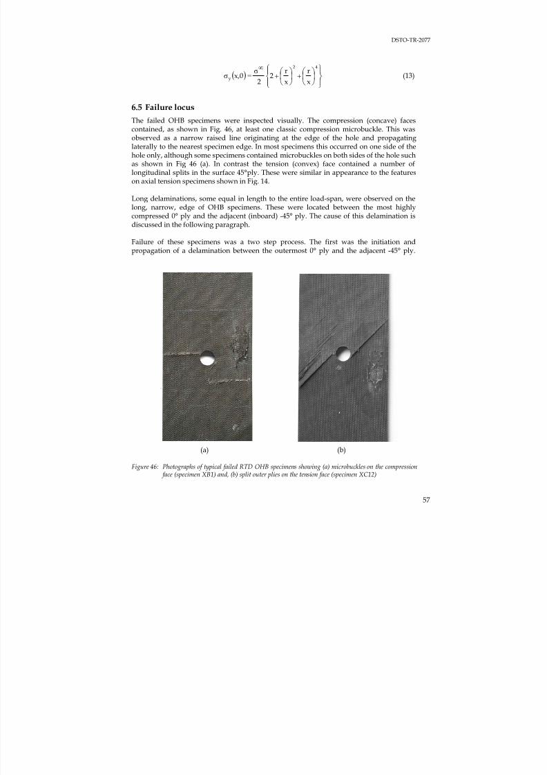
7/31/2019 Effect Hole Size Env Callus DSTO TR 2077
http://slidepdf.com/reader/full/effect-hole-size-env-callus-dsto-tr-2077 67/82
DSTO-TR-2077
57
( )⎪⎭
⎪⎬⎫
⎪⎩
⎪⎨⎧
⎟ ⎠
⎞⎜⎝
⎛ ⎟ ⎠
⎞⎜⎝
⎛ = ++∞σ
σ42
yx
r
x
r2
2x,0 (13)
6.5 Failure locus
The failed OHB specimens were inspected visually. The compression (concave) facescontained, as shown in Fig. 46, at least one classic compression microbuckle. This wasobserved as a narrow raised line originating at the edge of the hole and propagatinglaterally to the nearest specimen edge. In most specimens this occurred on one side of thehole only, although some specimens contained microbuckles on both sides of the hole suchas shown in Fig 46 (a). In contrast the tension (convex) face contained a number oflongitudinal splits in the surface 45°ply. These were similar in appearance to the featureson axial tension specimens shown in Fig. 14.
Long delaminations, some equal in length to the entire load-span, were observed on thelong, narrow, edge of OHB specimens. These were located between the most highlycompressed 0° ply and the adjacent (inboard) -45° ply. The cause of this delamination isdiscussed in the following paragraph.
Failure of these specimens was a two step process. The first was the initiation andpropagation of a delamination between the outermost 0° ply and the adjacent -45° ply.
(a) (b)
Figure 46: Photographs of typical failed RTD OHB specimens showing (a) microbuckles on the compression face (specimen XB1) and, (b) split outer plies on the tension face (specimen XC12)
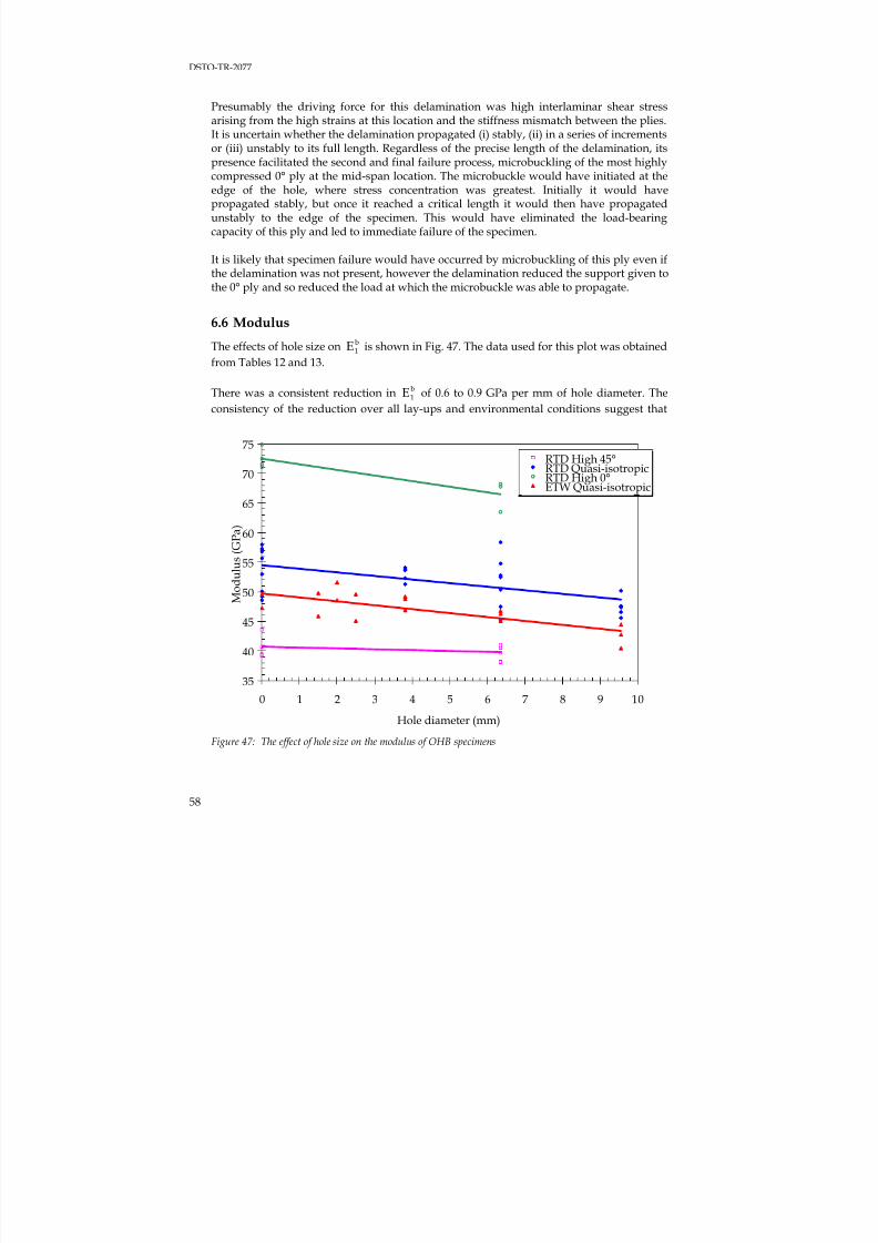
7/31/2019 Effect Hole Size Env Callus DSTO TR 2077
http://slidepdf.com/reader/full/effect-hole-size-env-callus-dsto-tr-2077 68/82
DSTO-TR-2077
58
Presumably the driving force for this delamination was high interlaminar shear stressarising from the high strains at this location and the stiffness mismatch between the plies.It is uncertain whether the delamination propagated (i) stably, (ii) in a series of increments
or (iii) unstably to its full length. Regardless of the precise length of the delamination, itspresence facilitated the second and final failure process, microbuckling of the most highlycompressed 0° ply at the mid-span location. The microbuckle would have initiated at theedge of the hole, where stress concentration was greatest. Initially it would havepropagated stably, but once it reached a critical length it would then have propagatedunstably to the edge of the specimen. This would have eliminated the load-bearingcapacity of this ply and led to immediate failure of the specimen.
It is likely that specimen failure would have occurred by microbuckling of this ply even ifthe delamination was not present, however the delamination reduced the support given tothe 0° ply and so reduced the load at which the microbuckle was able to propagate.
6.6 Modulus
The effects of hole size on b1E is shown in Fig. 47. The data used for this plot was obtained
from Tables 12 and 13.
There was a consistent reduction in b1E of 0.6 to 0.9 GPa per mm of hole diameter. The
consistency of the reduction over all lay-ups and environmental conditions suggest that
Figure 47: The effect of hole size on the modulus of OHB specimens
35
40
45
50
55
60
65
70
75
0 1 2 3 4 5 6 7 8 9 10
Hole diameter (mm)
M o d u l u s ( G P a )
RTD High 45°RTD Quasi-isotropicRTD High 0°ETW Quasi-isotropic
°
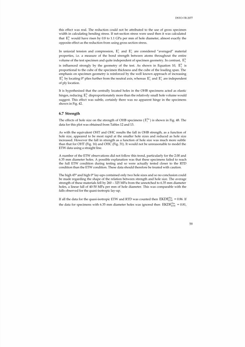
7/31/2019 Effect Hole Size Env Callus DSTO TR 2077
http://slidepdf.com/reader/full/effect-hole-size-env-callus-dsto-tr-2077 69/82
DSTO-TR-2077
59
this effect was real. The reduction could not be attributed to the use of gross specimenwidth in calculating bending stress. If net-section stress were used then it was calculated
that b1E would have risen by 0.8 to 1.1 GPa per mm of hole diameter, almost exactly the
opposite effect as the reduction from using gross section stress.
In uniaxial tension and compression, t1E and c
1E are considered “averaged” material
properties, i.e. a measure of the bond strength between atoms throughout the entire
volume of the test specimen and quite independent of specimen geometry. In contrast, b1E
is influenced strongly by the geometry of the test. As shown in Equation 10, b1E is
proportional to the cube of the specimen thickness and the cube of the loading span. Theemphasis on specimen geometry is reinforced by the well known approach of increasing
b1E by locating 0° plies further from the neutral axis, whereas t
1E and c1E are independent
of ply location.
It is hypothesised that the centrally located holes in the OHB specimens acted as elastic
hinges, reducing b1E disproportionately more than the relatively small hole volume would
suggest. This effect was subtle, certainly there was no apparent hinge in the specimensshown in Fig. 42.
6.7 Strength
The effects of hole size on the strength of OHB specimens ( bu1F ) is shown in Fig. 48. The
data for this plot was obtained from Tables 12 and 13.
As with the equivalent OHT and OHC results the fall in OHB strength, as a function ofhole size, appeared to be most rapid at the smaller hole sizes and reduced as hole sizeincreased. However the fall in strength as a function of hole size was much more subtlethan that for OHT (Fig. 16) and OHC (Fig. 31). It would not be unreasonable to model theETW data using a straight line.
A number of the ETW observations did not follow this trend, particularly for the 2.00 and6.35 mm diameter holes. A possible explanation was that these specimens failed to reachthe full ETW condition during testing and so were actually tested closer to the RTDcondition than the ETW condition. These data should therefore be treated with caution.
The high 45° and high 0° lay-ups contained only two hole sizes and so no conclusion couldbe made regarding the shape of the relation between strength and hole size. The averagestrength of these materials fell by 260 – 325 MPa from the unnotched to 6.35 mm diameterholes, a linear fall of 40-50 MPa per mm of hole diameter. This was comparable with thefalls observed for the quasi-isotropic lay-up.
If all the data for the quasi-isotropic ETW and RTD was counted then FbuETWEKDF = 0.86. If
the data for specimens with 6.35 mm diameter holes was ignored then FbuETWEKDF = 0.81,
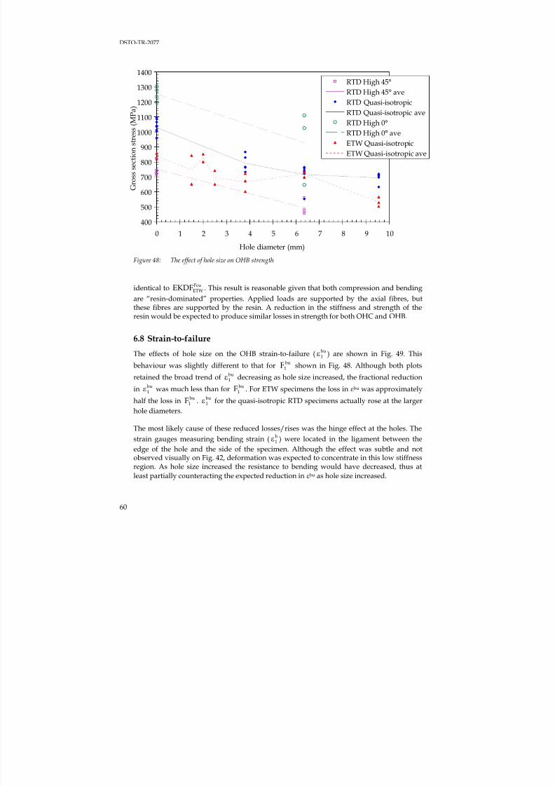
7/31/2019 Effect Hole Size Env Callus DSTO TR 2077
http://slidepdf.com/reader/full/effect-hole-size-env-callus-dsto-tr-2077 70/82
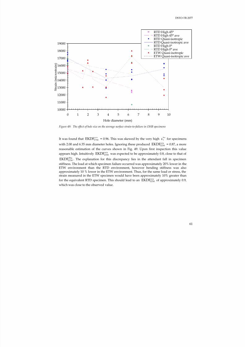
7/31/2019 Effect Hole Size Env Callus DSTO TR 2077
http://slidepdf.com/reader/full/effect-hole-size-env-callus-dsto-tr-2077 71/82
DSTO-TR-2077
61
Figure 49: The effect of hole size on the average surface strain-to-failure in OHB specimens
It was found that cuETWEKDFε = 0.96. This was skewed by the very high bu
1ε for specimens
with 2.00 and 6.35 mm diameter holes. Ignoring these produced cuETWEKDFε = 0.87, a more
reasonable estimation of the curves shown in Fig. 49. Upon first inspection this value
appears high. Intuitively cuETWEKDFε was expected to be approximately 0.8, close to that of
FbuETWEKDF . The explanation for this discrepancy lies in the attendant fall in specimen
stiffness. The load at which specimen failure occurred was approximately 20% lower in theETW environment than the RTD environment, however bending stiffness was also
approximately 10 % lower in the ETW environment. Thus, for the same load or stress, thestrain measured in the ETW specimen would have been approximately 10% greater than
for the equivalent RTD specimen. This should lead to an cuETWEKDFε of approximately 0.9,
which was close to the observed value.
10000
11000
12000
13000
14000
15000
16000
17000
18000
19000
0 1 2 3 4 5 6 7 8 9 10
Hole diameter (mm)
S t r a i n ( m i c r o s t r a i n )
RTD High 45°RTD High 45° aveRTD Quasi-isotropic
RTD Quasi-isotropic aveRTD High 0°RTD High 0° aveETW Quasi-isotropicETW Quasi-isotropic ave

7/31/2019 Effect Hole Size Env Callus DSTO TR 2077
http://slidepdf.com/reader/full/effect-hole-size-env-callus-dsto-tr-2077 72/82
DSTO-TR-2077
62
6.9 Strength prediction
6.9.1 Average Stress Criterion
The average unnotched compression strength was calculated from the data in Tables 12and 13.
Assuming that Equation 1 modelled the stress distribution around the hole then the ratioof notched to unnotched strengths for the ASC was given by Equation 5. Modifying thestress distribution to Equation 13 changed the ASC to Equation 14.
( )42
3
1
3
2111
1N
2
12
ξ−ξ−ξ−
ξ−=
σ
σ
0
(14)
Where:
ξ1 =0ar
r
+
The a0 for both Equations 5 and 14 was calculated using least squares fits of theseequations with the experimental data.
The measured strength of ETW specimens with 6.35 mm diameter holes appeared veryhigh. Ignoring the results for these specimens and repeating the least square fit yieldedmoderate improvements in the determination coefficient when compared to using the full
data set. It was judged that the smaller data set was a more realistic representation of thereal OHB behaviour and so the parameters obtained from these regressions were used.
The resultant parameters are shown below while the experimental data and curves of bestfit are shown in Fig. 50:
Equation 5RTD σ0 = 1029 MPa a0 = 7.49 mm R2 = 0.777
ETW σ0 = 839 MPa a0 = 10.33 mm R2 = 0.506 Full data set
σ0 = 839 MPa a0 = 7.93 mm R2 = 0.682 Ignoring 6.35 mm holes
Equation 14RTD σ0 = 1029 MPa a0 = 3.63 mm R2 = 0.814
ETW σ0 = 839 MPa a0 = 5.70 mm R2 = 0.503 Full data set
σ0 = 839 MPa a0 = 4.27 mm R2 = 0.670 Ignoring 6.35 mm holes
Scatter in the data made it difficult to determine whether the model derived from the morerealistic model of strain distribution (Equation 14) improved the prediction of strength. R2 increased moderately for the RTD data but decreased slightly for the ETW data. In theabsence of conclusive data, it was judged to be more appropriate to use a model thatreflected the experimentally measured strains and thus the parameters from Equation 14were selected as most representing the real OHB behaviour.
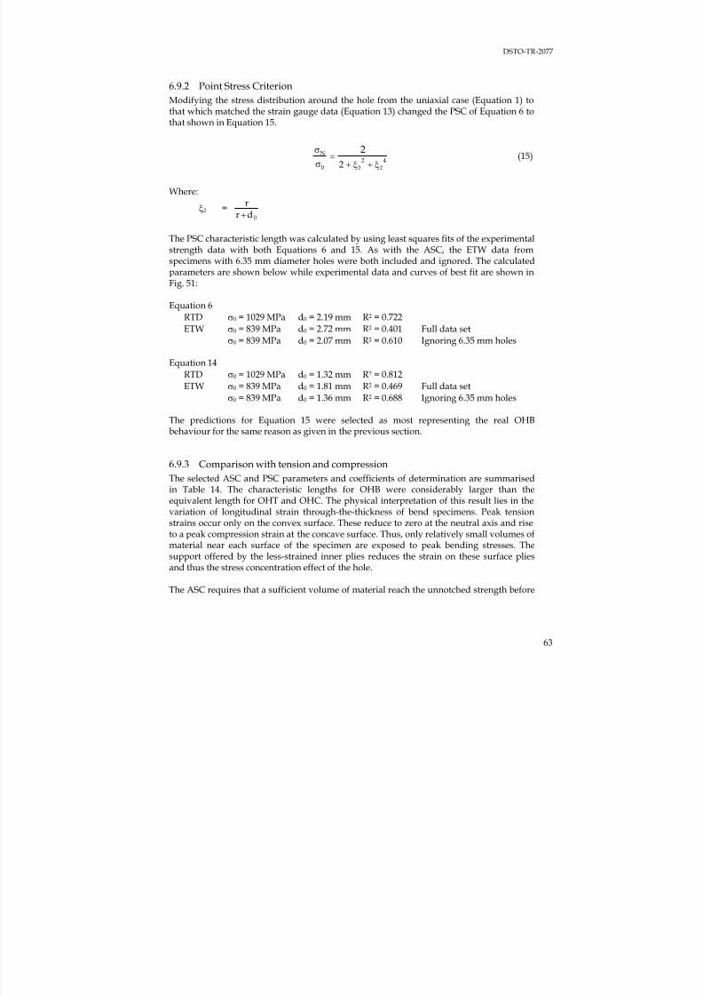
7/31/2019 Effect Hole Size Env Callus DSTO TR 2077
http://slidepdf.com/reader/full/effect-hole-size-env-callus-dsto-tr-2077 73/82
DSTO-TR-2077
63
6.9.2 Point Stress Criterion
Modifying the stress distribution around the hole from the uniaxial case (Equation 1) tothat which matched the strain gauge data (Equation 13) changed the PSC of Equation 6 to
that shown in Equation 15.
4
2
2
20
N
2
2
ξ+ξ+σ
σ= (15)
Where:
ξ2 =0dr
r
+
The PSC characteristic length was calculated by using least squares fits of the experimentalstrength data with both Equations 6 and 15. As with the ASC, the ETW data fromspecimens with 6.35 mm diameter holes were both included and ignored. The calculatedparameters are shown below while experimental data and curves of best fit are shown inFig. 51:
Equation 6
RTD σ0 = 1029 MPa d0 = 2.19 mm R2 = 0.722
ETW σ0 = 839 MPa d0 = 2.72 mm R2 = 0.401 Full data set
σ0 = 839 MPa d0 = 2.07 mm R2 = 0.610 Ignoring 6.35 mm holes
Equation 14
RTD σ0 = 1029 MPa d0 = 1.32 mm R2 = 0.812
ETW σ0 = 839 MPa d0 = 1.81 mm R2 = 0.469 Full data set
σ0 = 839 MPa d0 = 1.36 mm R2 = 0.688 Ignoring 6.35 mm holes
The predictions for Equation 15 were selected as most representing the real OHBbehaviour for the same reason as given in the previous section.
6.9.3 Comparison with tension and compression
The selected ASC and PSC parameters and coefficients of determination are summarised
in Table 14. The characteristic lengths for OHB were considerably larger than theequivalent length for OHT and OHC. The physical interpretation of this result lies in thevariation of longitudinal strain through-the-thickness of bend specimens. Peak tensionstrains occur only on the convex surface. These reduce to zero at the neutral axis and riseto a peak compression strain at the concave surface. Thus, only relatively small volumes ofmaterial near each surface of the specimen are exposed to peak bending stresses. Thesupport offered by the less-strained inner plies reduces the strain on these surface pliesand thus the stress concentration effect of the hole.
The ASC requires that a sufficient volume of material reach the unnotched strength before
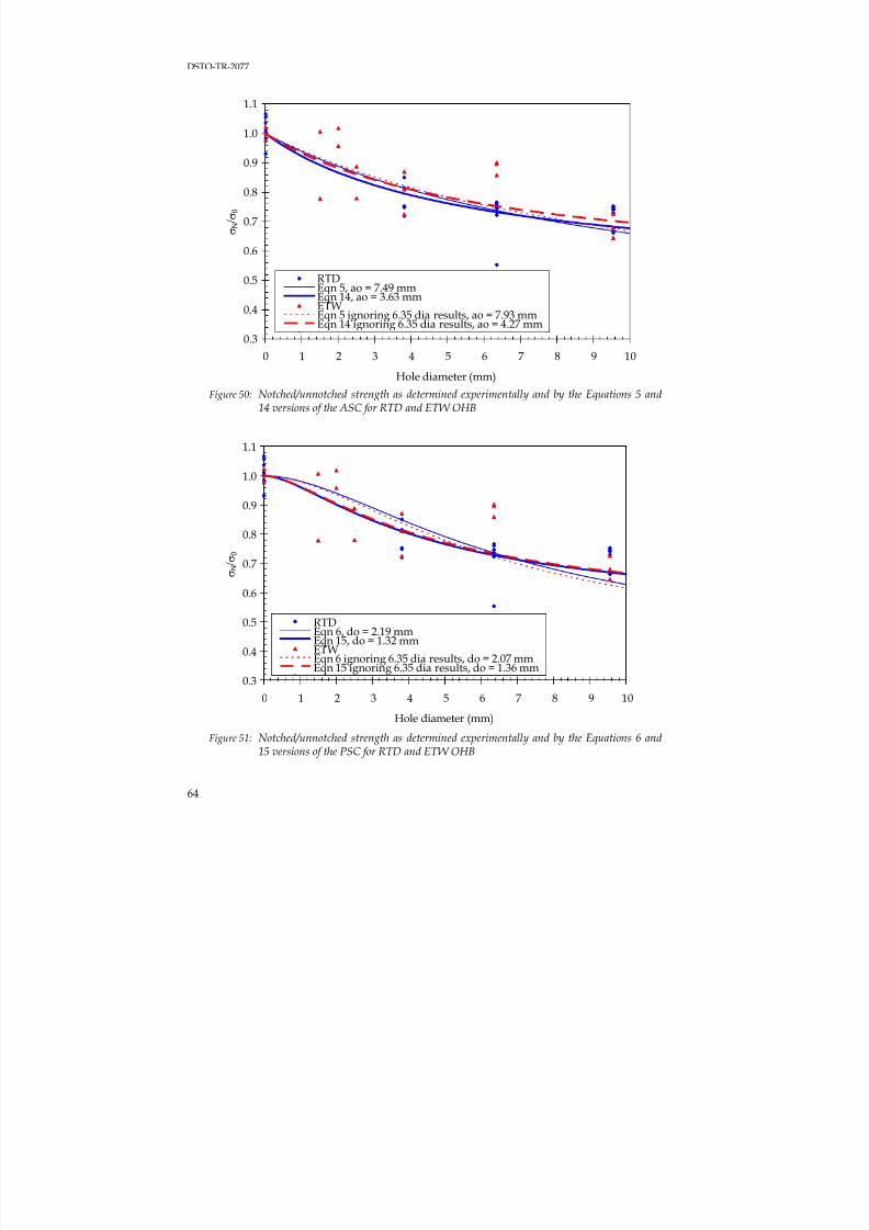
7/31/2019 Effect Hole Size Env Callus DSTO TR 2077
http://slidepdf.com/reader/full/effect-hole-size-env-callus-dsto-tr-2077 74/82
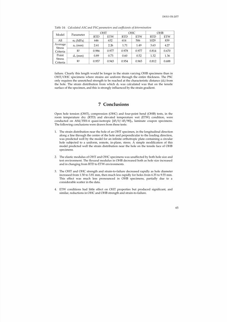
7/31/2019 Effect Hole Size Env Callus DSTO TR 2077
http://slidepdf.com/reader/full/effect-hole-size-env-callus-dsto-tr-2077 75/82
DSTO-TR-2077
65
Table 14: Calculated ASC and PSC parameters and coefficients of determination
OHT OHC OHBModel Parameter
RTD ETW RTD ETW RTD ETW
All σ0 (MPa) 646 632 614 506 1029 839
ao (mm) 2.61 2.26 1.71 1.49 3.63 4.27AverageStress
Criteria R2 0.986 0.977 0.978 0.977 0.814 0.670
do (mm) 0.89 0.73 0.60 0.52 1.32 1.36PointStress
Criteria R2 0.957 0.943 0.954 0.965 0.812 0.688
failure. Clearly this length would be longer in the strain varying OHB specimens than inOHT/OHC specimens where strains are uniform through the entire thickness. The PSC
only requires the unnotched strength to be reached at the characteristic distance (d0) fromthe hole. The strain distribution from which d0 was calculated was that on the tensilesurface of the specimen, and this is strongly influenced by the strain gradient.
7 Conclusions
Open hole tension (OHT), compression (OHC) and four-point bend (OHB) tests, in theroom temperature dry (RTD) and elevated temperature wet (ETW) condition, wereconducted on AS4/3501-6 quasi-isotropic [45/0/-45/90]2s laminate coupon specimens.The following conclusions were drawn from these tests:
1. The strain distribution near the hole of an OHT specimen, in the longitudinal directionalong a line through the centre of the hole and perpendicular to the loading direction,was predicted well by the model for an infinite orthotropic plate containing a circularhole subjected to a uniform, remote, in-plane, stress. A simple modification of thismodel predicted well the strain distribution near the hole on the tensile face of OHBspecimens.
2. The elastic modulus of OHT and OHC specimens was unaffected by both hole size andtest environment. The flexural modulus in OHB decreased both as hole size increasedand in changing from RTD to ETW environments.
3. The OHT and OHC strength and strain-to-failure decreased rapidly as hole diameterincreased from 1.50 to 3.81 mm, then much less rapidly for holes from 6.35 to 9.55 mm.This effect was much less pronounced in OHB specimens, partially due to aconsiderable scatter in the data.
4. ETW conditions had little effect on OHT properties but produced significant, andsimilar, reductions in OHC and OHB strength and strain-to-failure.
7/31/2019 Effect Hole Size Env Callus DSTO TR 2077
http://slidepdf.com/reader/full/effect-hole-size-env-callus-dsto-tr-2077 76/82
DSTO-TR-2077
66
5. The deflection OHB specimens with 0.00 and 6.35 mm diameter holes was representedwell by assuming no hole and using classical beam deflection theory.
6. OHT and OHC strength was predicted very well, and OHB strength moderately well,by the Whitney-Nuismer Average Stress Criterion and Point Stress Criterion whenusing the strain distribution for that specimen type. OHC strength was also predictedvery well by the Budiansky-Soutis-Fleck Cohesive Zone Model. It is suspected thatthese models will not predict accurately the strength of coupons subject to combinedaxial and bend loading
8 Acknowledgments
The author acknowledges the contributions of Leo Mirabella (DSTO) for conducting andorganising a number of the tests, Michael Bannister (CRC-ACS) for project management,Peter Haggart (Fortburn Pty Ltd) for specimen manufacture, and Mark McVilley (CRC-ACS), Neil Absolom, Rodney Gray and David Parslow are for their contribution to straingauging and testing.
9 References
1 Whitney, J. M. and Nuismer, R. J., ”Stress fracture criteria for laminated compositescontaining stress concentrations”, Journal of Composite Materials, Vol. 8, 1974, pp.253-265.
2 Konish, H. J. and Whitney, J. M., ”Approximate stresses in an orthotropic platecontaining a circular hole”, Journal of Composite Materials, Vol. 9, 1975, pp. 157-166.
3 Lekhnitskii, S. G., “Anisotropic plates”, Translated from the Second Russian Editionby S. W. Tsai and T. Cheron, Gordon and Breach Science Publishers Inc., New York,1968.
4 Davis, M. J. and Jones, R., “Damage tolerance of fibre composite laminates incomposites for aircraft structures”, Chapter 10, Editors B.C. Hoskin and A.A. Baker,Education Series 1986.
5 Soutis, C., Fleck, N. A. and Smith, P. A., “Failure prediction technique for compressionloaded carbon fibre-epoxy laminate with open holes”, Journal of Composite Materials,Vol. 25, November 1991, pp. 1476-1498.
6 Tan, S., “Finite-width correction factor for anisotropic plate containing a centralopening”, Journal pf Composite Materials, Vol. 22, 1988, pp. 1080-1097.
7/31/2019 Effect Hole Size Env Callus DSTO TR 2077
http://slidepdf.com/reader/full/effect-hole-size-env-callus-dsto-tr-2077 77/82
DSTO-TR-2077
67
7 Jones, R. M., “Mechanics of composite materials”, Scripta Book Co., Washington, D.C., 1975.
8 Suppliers of Advanced Composite Materials, “SACMA recommended test method foropen-hole tensile properties of oriented fiber-resin composites”, SACMA SRM 5R–94in SACMA Recommended Methods, Composites Fabricators Association, 1999, 8 pp.
9 Suppliers of Advanced Composite Materials, “SACMA recommended test method foropen-hole compression properties of oriented fiber-resin composites”, SACMA SRM3R–94, in SACMA Recommended Methods, Composites Fabricators Association, 1999,10 pp.
10 ASTM Standard D790, “Standard test method for flexure properties of unreinforced
and reinforced plastics and electrical insulating materials”, ASTM International, WestConshohocken, PA, www.astm.org
11 Callus, P. J., Mouritz, A. P., Bannister, M. K. and Leong, K. H., “Tensile properties andfailure mechanisms of 3D woven GRP composites”, Composites, 30A, June, 1999, pp.1277-1287.
12 http://www.graphpad.com/curvefit/2_models__1_dataset.htm
13 Potti, P. K. G., Rao, B. N. and Srivastava, V. K., “Notched tensile strength of randomlyoriented E-glass composite laminates”, Materials Science and Engineering, A282, 2000,pp. 59-66.
14 Komadina, J., Sheppard, A., Callus, P. J. and Bannister, M., “BAE Systems/DSTOcollaboration: Uniaxial coupon loading (WP2)”, CRC-ACS-TM-01022, CooperativeResearch Centre for Advanced Composite Structures, Melbourne, Australia, October2001, 25 pp.
15 Sutcliffe, M. P. F., Xin, X. J., Fleck, N. A., Curtis, P. T., “Composite CompressiveStrength Modeller”, Version 1.4a, 1999, Engineering Department, CambridgeUniversity, Trumpington St, Cambridge, CB2 1PZ, E-mail: [email protected]
16 Adams, D. F., “Flexure test methods”, High Performance Composites, November,2005, 2 pp., http://www.compositesworld.com/hpc/issues/2005/November/1050

7/31/2019 Effect Hole Size Env Callus DSTO TR 2077
http://slidepdf.com/reader/full/effect-hole-size-env-callus-dsto-tr-2077 78/82
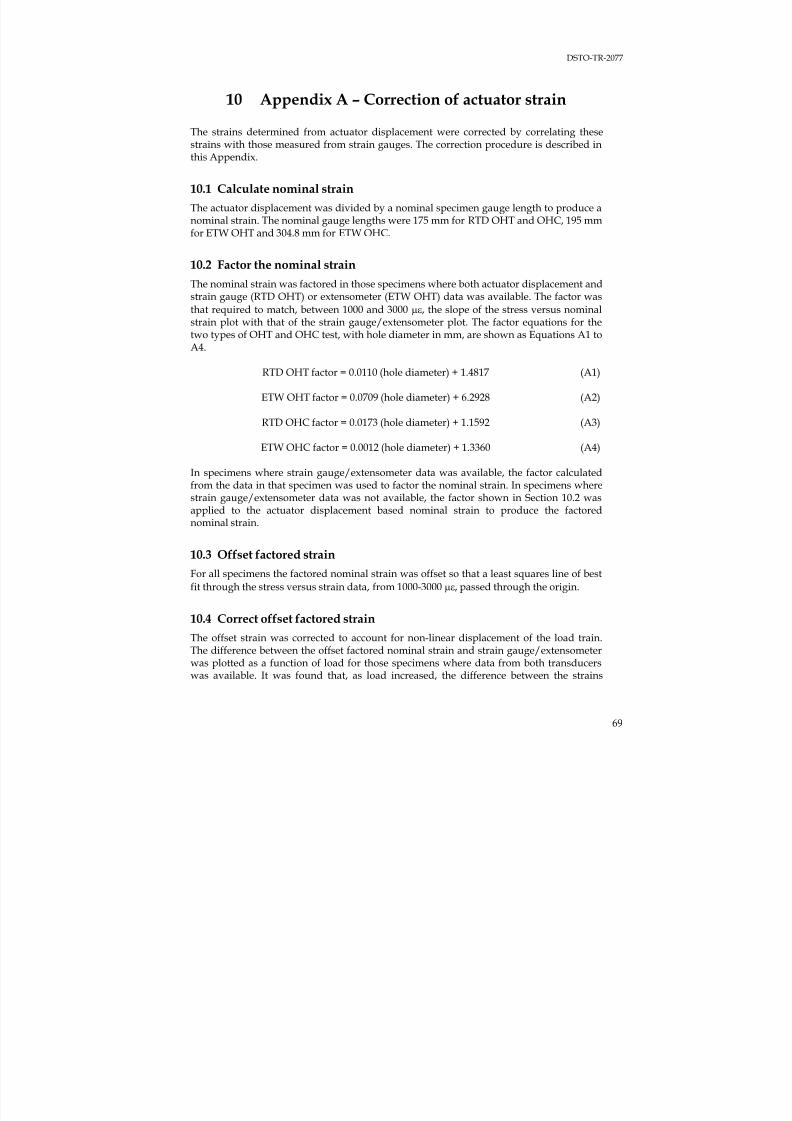
7/31/2019 Effect Hole Size Env Callus DSTO TR 2077
http://slidepdf.com/reader/full/effect-hole-size-env-callus-dsto-tr-2077 79/82
DSTO-TR-2077
69
10 Appendix A – Correction of actuator strain
The strains determined from actuator displacement were corrected by correlating thesestrains with those measured from strain gauges. The correction procedure is described inthis Appendix.
10.1 Calculate nominal strain
The actuator displacement was divided by a nominal specimen gauge length to produce anominal strain. The nominal gauge lengths were 175 mm for RTD OHT and OHC, 195 mmfor ETW OHT and 304.8 mm for ETW OHC.
10.2 Factor the nominal strain
The nominal strain was factored in those specimens where both actuator displacement andstrain gauge (RTD OHT) or extensometer (ETW OHT) data was available. The factor wasthat required to match, between 1000 and 3000 με, the slope of the stress versus nominalstrain plot with that of the strain gauge/extensometer plot. The factor equations for thetwo types of OHT and OHC test, with hole diameter in mm, are shown as Equations A1 toA4.
RTD OHT factor = 0.0110 (hole diameter) + 1.4817 (A1)
ETW OHT factor = 0.0709 (hole diameter) + 6.2928 (A2)
RTD OHC factor = 0.0173 (hole diameter) + 1.1592 (A3)
ETW OHC factor = 0.0012 (hole diameter) + 1.3360 (A4)
In specimens where strain gauge/extensometer data was available, the factor calculatedfrom the data in that specimen was used to factor the nominal strain. In specimens wherestrain gauge/extensometer data was not available, the factor shown in Section 10.2 wasapplied to the actuator displacement based nominal strain to produce the factorednominal strain.
10.3 Offset factored strainFor all specimens the factored nominal strain was offset so that a least squares line of best
fit through the stress versus strain data, from 1000-3000 με, passed through the origin.
10.4 Correct offset factored strain
The offset strain was corrected to account for non-linear displacement of the load train.The difference between the offset factored nominal strain and strain gauge/extensometerwas plotted as a function of load for those specimens where data from both transducerswas available. It was found that, as load increased, the difference between the strains
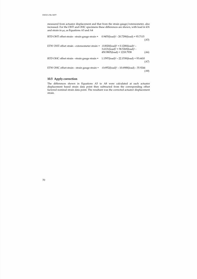
7/31/2019 Effect Hole Size Env Callus DSTO TR 2077
http://slidepdf.com/reader/full/effect-hole-size-env-callus-dsto-tr-2077 80/82
DSTO-TR-2077
70
measured from actuator displacement and that from the strain gauge/extensometer, alsoincreased. For the OHT and OHC specimens these differences are shown, with load in kN
and strain in με, as Equations A3 and A4
RTD OHT offset strain - strain gauge strain = 0.9455(load)2 - 20.7290(load) + 93.7115(A5)
ETW OHT offset strain - extensometer strain = -0.0020(load)5 + 0.1200(load)4 –3.6121(load)3 + 58.5269(load)2 -450.9805(load) + 1218.7938 (A6)
RTD OHC offset strain - strain gauge strain = 1.1597(load)2 – 22.1530(load) + 93.6410(A7)
ETW OHC offset strain - strain gauge strain = -0.6952(load)2
– 10.6908(load) – 35.9244(A8)
10.5 Apply correction
The differences shown in Equations A5 to A8 were calculated at each actuatordisplacement based strain data point then subtracted from the corresponding offsetfactored nominal strain data point. The resultant was the corrected actuator displacementstrain.
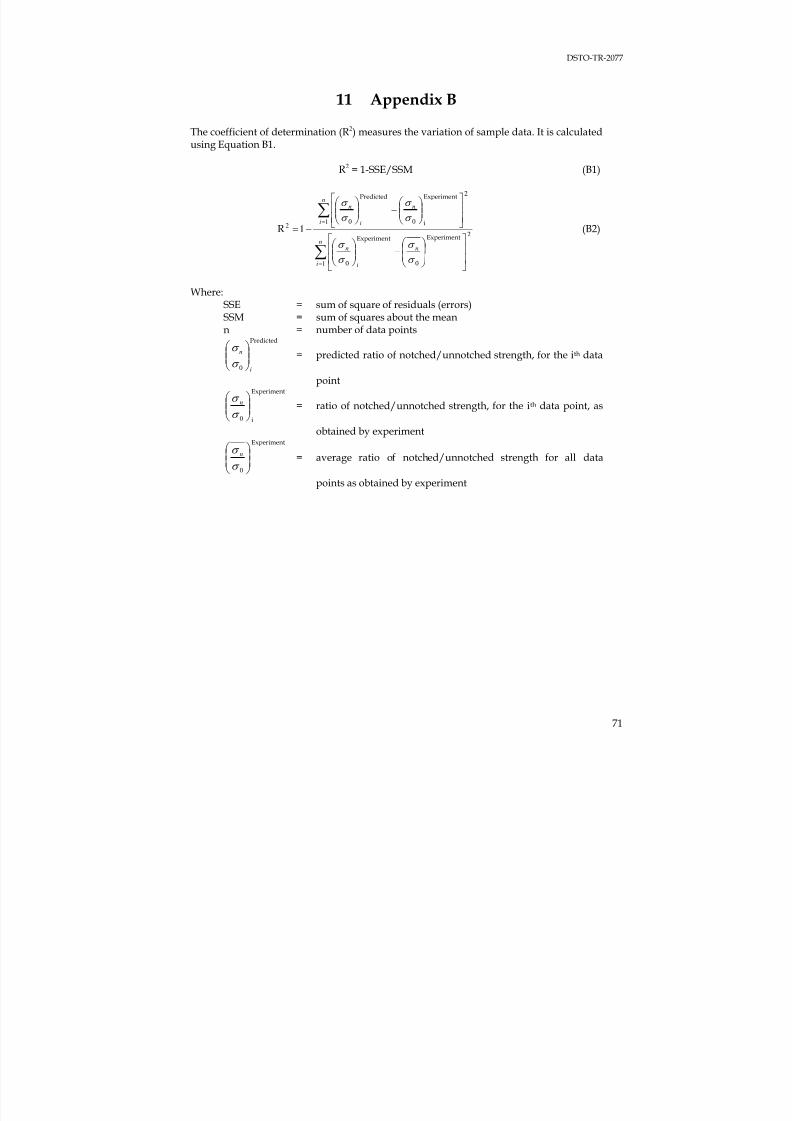
7/31/2019 Effect Hole Size Env Callus DSTO TR 2077
http://slidepdf.com/reader/full/effect-hole-size-env-callus-dsto-tr-2077 81/82
DSTO-TR-2077
71
11 Appendix B
The coefficient of determination (R2) measures the variation of sample data. It is calculatedusing Equation B1.
R2 = 1-SSE/SSM (B1)
∑
∑
=
=
⎥⎥
⎦
⎤
⎢⎢
⎣
⎡
⎟⎟ ⎠
⎞⎜⎜⎝
⎛ −⎟⎟
⎠
⎞⎜⎜⎝
⎛
⎥⎥
⎦
⎤
⎢⎢
⎣
⎡
⎟⎟ ⎠
⎞⎜⎜⎝
⎛ −⎟⎟
⎠
⎞⎜⎜⎝
⎛
−=n
i
n
i
n
n
i
n
i
n
1 00
1 002
12ExperimentExperiment
2Experiment
i
Predicted
R
σ
σ
σ
σ
σ
σ
σ
σ
(B2)
Where:SSE = sum of square of residuals (errors)SSM = sum of squares about the meann = number of data points
Predicted
i
n
⎟⎟ ⎠
⎞⎜⎜⎝
⎛
0σ
σ = predicted ratio of notched/unnotched strength, for the ith data
pointExperiment
i⎟
⎟
⎠
⎞
⎜
⎜
⎝
⎛
0σ
σ n = ratio of notched/unnotched strength, for the ith data point, as
obtained by experimentExperiment
⎟⎟ ⎠
⎞⎜⎜⎝
⎛
0σ
σ n = average ratio of notched/unnotched strength for all data
points as obtained by experiment
7/31/2019 Effect Hole Size Env Callus DSTO TR 2077
http://slidepdf.com/reader/full/effect-hole-size-env-callus-dsto-tr-2077 82/82
Page classification: UNCLASSIFIED
DEFENCE SCIENCE AND TECHNOLOGY ORGANISATION
DOCUMENT CONTROL DATA 1. PRIVACY MARKING/CAVEAT (OF DOCUMENT)
2. TITLE
The Effects of Hole-size and Environment on the MechanicalBehaviour of a Quasi-isotropic AS4/3501-6 Laminate in Tension,Compression and Bending
3. SECURITY CLASSIFICATION (FOR UNCLASSIFIED REPORTSTHAT ARE LIMITED RELEASE USE (L) NEXT TO DOCUMENTCLASSIFICATION)
Document (U)Title (U)Abstract (U)
4. AUTHOR(S)
Paul J. Callus
5. CORPORATE AUTHOR
DSTO Defence Science and Technology Organisation506 Lorimer St
Fishermans Bend Victoria 3207 Australia 6a. DSTO NUMBER
DSTO-TR-20776b. AR NUMBER
AR-014-060
6c. TYPE OF REPORT
Technical Report 7. DOCUMENT DATE
November 2007
8. FILE NUMBER
2007/1125658/19. TASK NUMBER
AIR 07/05310. TASK SPONSOR
DGTA
11. NO. OF PAGES
72
12. NO. OF REFERENCES
16
13. DOWNGRADING/DELIMITING INSTRUCTIONS
http://www.dsto.defence.gov.au/corporate/reports/DSTO-TR-2077.pdf
14. RELEASE AUTHORITY
Chief, Air Vehicles Division
15. SECONDARY RELEASE STATEMENT OF THIS DOCUMENT
Approved for public release
OVERSEAS ENQUIRIES OUTSIDE STATED LIMITATIONS SHOULD BE REFERRED THROUGH DOCUMENT EXCHANGE, PO BOX 1500, EDINBURGH, SA 5111
16. DELIBERATE ANNOUNCEMENT
No Limitations
17. CITATION IN OTHER DOCUMENTS Yes
18. DEFTEST DESCRIPTORS
Carbon fibre reinforced compositesMechanical propertiesEnvironmentsStrainsFailure analysis
19. ABSTRACT
This report describes the results of open-hole-tension (OHT), open-hole-compression (OHC) and open-hole-four-point-bend (OHB)tests conducted on AS4/3501-6 quasi-isotropic [45/0/-45/90]2s laminates in the room temperature dry (RTD) and elevated temperaturewet (ETW) condition. Specimens were 38.1 mm wide with central through-holes ranging in diameter from 0.00 (unnotched) to 9.55 mm.Th t i di t ib ti th h l i OHT i d d f d t ll ith th t di t d f i fi it