Effect of Different Yield Functions on Computations of

F. Mousavi et. al., Journal of Advanced Materials and Processing, Vol. 6, No. 3, 2018, 66-79 66

Effect of Different Yield Functions on Computations of Forming Limit

Curves for Aluminum Alloy Sheets

F. Mousavi, M. Erfanian, R. Hashemi, R. Madoliat

1 School of Mechanical Engineering, Iran University of Science and Technology.

ARTICLE INFO ABSTRACT

Article history:

Received 31 January 2017 Accepted 2 October 2018

Available online 5 November 2018

In this article, the effect of different yield functions on the prediction

of forming limit diagram (FLD) for the aluminum sheet is studied.

Due to the importance of FLD in sheet metal forming, concentration

on effective parameters must be considered precisely to have better

theoretical prediction comparing experimental results. Yield

function is one of the factors that can be improved by adding new

coefficients and consequently follows the behaviour of material with

good approximation. Therefor applying different yield functions can

change shape and level of FLDs. In this study the yield criteria which

are used in the determination of forming limit curves, are Hill48,

Hosford, BBC2008, Soare2008, Plunkett2008 and Yld2011. The

Yld2011 yield function is more appropriate than the other yield

functions for prediction of the FLD of aluminum alloy. The well-

known Marciniak-Kuczynski (M-K) theory and voce hardening law

have also been used. To verify the numerical results, the obtained

results have been compared with available experimental data.

Keywords:

Forming limit diagram

Aluminum

Yield functions

Marciniak-Kuczynski theory

1-Introduction

Sheet metal can sustain the limited amount of

stretch during forming due to occurrence of

localized neck. Forming limit diagram (FLD) is

a tool which can be used to detect the initiation

of necking [1,2]. Generating FLD with

experimental methods needs a lot of time and

cost, so obtaining them by theoretical methods

with good accuracy is really essential in metal

forming. One of the mathematical methods that

is useful in generating FLD is Marciniak-

Kuczynski (M-K) theory [3,4]. A lot of

researches have been done by using this model

to consider the effect of different factors consist

of anisotropy coefficient, inhomogeneous

coefficient, principal strain, strain hardening

exponent, strain rate and various yield criteria in

predicting FLD [4,5]. Yield function describes

the behavior of material, so each type of metal

can be described better with a special kind of

yield criterion. It means that this yield criterion

Corresponding author:

E-mail address: [email protected]

can predict limit strains more accurately and

better predictions of FLDs will be obtained in

comparison by experimental ones.

Effect of different yield criteria on the

computation of forming limit diagram has been

the subject of several researches. For instance,

Butut et al. [5] studied the effect of two yield

functions, Yld96 and BBC2000, on predicting

FLD for orthotropic metal sheets under plane

strain condition. Also, they considered effect of

anisotropy coefficient on FLD for AA5XXX by

M-K model and voce hardening law and by

using these two yield functions. Ganjiani and

Assempour [6] studied Hosford and BBC2000

in conjunction with the M-K model, they

showed that 6th exponent of Hosford yield

criterion for AK steel and 8th exponent of

Hosford and BBC2000 for AA5XXX were

appropriate refer to experimental results.

Ahmadi et al. [7] obtained FLD for AA3003-O


by using the M-K model and voce and swift

hardening law.

Consequently, they claimed that BBC2003 and

the Voce law hardening were suitable for

AA3003-O. Yoon et al. [8] obtained FLD for

AA5042-H2 by using the anisotropy yield

function Yld2000-2D and a form of CPB06ex2

yield function and voce work hardening law.

Rezaie bazzaz et al. [9] focused on the effect of

strain hardening exponent and strain rate in FLD

of IF steel, AA3003-O and AA8014-O by Hill

93 yield criterion.

Consequently, found out increasing these

parameters cause more formability. Dasappa et

al. [10] reported FLD of AA5754 by using five

yield criteria to consist of Hill48, Hill90, Hill93,

Yld89 and Plunkett 2008. They achieved that

prediction of forming limit diagram strongly

related to yield criteria and material parameters.

Xiaoqiang et al [11] consider von Mises, Hill48

and Yld89 in the prediction of FLD for Al-Li

2198-T3, and discovered that Hosford yield

function for the left side and Hill48 for the right

side of the diagram is suitable according to

experimental data. Panich et al. [12] studied

forming limit stress diagram and forming limit

diagram of two kinds of high strength steel,

DP780 and TPIR780, which were modeled with

von Mises, Hill48 and Yld2000 yield criteria

and voce and swift hardening laws. They

confirmed that hardening law and yield criterion

are effective parameters in the prediction of

forming limit diagram. Aretz et al. [13]

demonstrated the ability of Yld2011-18p and

Yld2011-27p yield functions in describing

complex plastic orthotropy of sheet metals.

Panich et al. [14] determined experimental

FLDs of the AHS steel grade DP980 by the

Nakazima stretch-forming test. Then, theoretical

FLDs according to the M-K model were

calculated using the Swift hardening law

coupled with the Yld2000-2d, Yld89 stress

based, Yld89 strain based, Hill’48 stress based

and Hill’48 strain based yield criteria.

These days, aluminum alloys are used a lot in

sheet forming industry. Therefore, having

enough information around formability of them

is essential. One of the useful applications in this

field is forming limit diagram. Due to lack of

suitable implementation of classic yield function

such as von Mises and Hill’s 48 to determine the

anisotropy plastic behavior and FLDs for

aluminum alloy sheet metals particularly, the

advanced yield criterion was introduced to

obtain satisfactory accuracy and agreement

between the theoretical and experimental

results.

In this research, the effect of several yield

functions (e.g., Hill48, Hosford, BBC2008,

Soare2008, Plunkett2008 and Yld2011) on the

prediction of forming limit diagrams for the five

kinds of aluminum alloy sheets are determined.

The methodology for computation of the FLDs

is based on the well-known M-K theory and the

Voce hardening law is also considered.

Consequently, the Yld2011 yield criterion

approximately describes the forming behavior

of aluminum sheet more accurately.

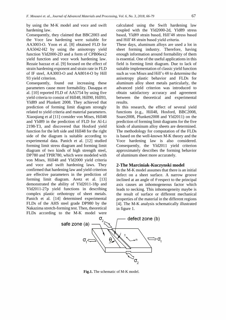
2-The Marciniak-Kuczynski model In the M-K model assumes that there is an initial

defect on a sheet surface. A narrow groove

inclined at an angle of θ respect to the principal

axis causes an inhomogeneous factor which

leads to necking. This inhomogeneity maybe is

the result of surface or different mechanical

properties of the material in the different regions

[4]. The M-K analysis schematically illustrated

in figure 1.

Fig.1. The schematic of M-K model.


The M-K model supposes that the sheet has two

regions: 1- homogeneous or safe region (a) and

t0a is the initial thickness of this zone, 2-

inhomogeneous or groove region with initial

thickness shown as t0b. It is necessary to state

that x, y, z -axes correspond to rolling,

transverse and normal sheet's directions,

whereas 1 and 2 show the principal stress and

strain directions in homogeneous region and the

groove region the axis represent by n, t, z. The

initial geometrical inhomogeneity is reported as

an initial defect factor that is shown by f0 and

characterized as the following form:

(1)

During plastic deformation, this defect factor

changes respect to below relation and shows this

factor is a function of the initial defect:

(2)

In above relation, 𝜖3 refers to strain along

thickness direction and calculated by relation

which is consisting of incompressibility

condition:

(3)

It is assumed that strains along the groove

direction are equal in two regions also during

deformation process, strain ratio which is

defined as minimum strain to maximum strain

inside the groove region decreases and in the

outside region of groove is constant

(proportional deformation). It can be claimed

that the groove deformation is close to plane

strain condition. By this condition, stress and

strain increments of groove zone can directly

obtained respect to their value in safe zone. The

main equations in the M-K model generate from

equilibrium and compatibility equations. For

finding the value of limit strains and stresses it

is assumed that the stress ratio, 𝜎𝑎

1

𝜎𝑎2, is constant.

At first step, all the strains are zero and the

loading on the safe zone started by assuming a

small value for d𝜖̅𝑎 (for instance d𝜖̅𝑎=0.0001)

and the equivalent strain, 𝜖̅𝑎, will be calculated.

(4)

The effective stress, �̅�𝑌, is obtained by

substituting the effective strain in the hardening

law. It is clear that the effective stresses which

are obtained from hardening law are equal to

those obtaining by yield function. Using the

assumed 𝑑𝜖̅𝑎 in the flow rule, stress and strain

components in the safe zone are calculated and

after that by using rotation matrix, T, the stress

and strain tensors are transformed to groove

coordinates using equations (5) and (6).

(5)

(6)

After calculation of safe zone's stress and strain

components, same variables must be calculated

in the groove zone. Unknown parameters in

groove region consist of 𝑑𝜖𝑏𝑡𝑡, 𝑑𝜖𝑏

𝑛𝑡, 𝑑𝜖𝑏𝑛𝑛,

𝜎𝑏𝑛𝑛, 𝜎𝑏

𝑡𝑡, 𝜎𝑏𝑛𝑡 stress increments are functions

of 𝑑𝜖̅𝑏, 𝜎𝑏𝑡𝑡, 𝜎𝑏

𝑛𝑛 and 𝜎𝑏𝑛𝑡. So, the unknown

parameters in this zone reduced to four

parameters (𝑑𝜖̅𝑏, 𝜎𝑏𝑛𝑛, 𝜎𝑏

𝑡𝑡 and 𝜎𝑏𝑛𝑡). The

force equilibrium equations in the groove's

normal and tangential directions can be written

as follows:

(7)

(8)

Changes that related to thickness in each step

can be expressed as a function of thickness

strain.

(9)

(10)

From equation (7) and (8) the force equilibrium

equations can be written as below forms:

(11)

(12)


Refer to compatibility equation, elongation in

both regions is equal:

(13)

Finally, the energy equilibrium relation written

as follows:

(14)

In equation (11), �̅�𝑌𝑏, is the effective stress of

groove zone that obtained by hardening law. So

three equations obtained from compatibility and

force equilibrium conditions and one other

equation from energy relation generated. These

four non-linear equations are as follows:

(15)

(16)

(17)

(18)

The unknown parameters and functions can be

defined as two vectors called X and F and come

at below:

(19)

(20)

In order to solve this non-linear system of

equations and calculating the unknown

parameters of the groove zone, the Newton-

Raphson method is applied. The general

procedure of this method explained in

following. The goal is solving system of

equations which include N functional relations

and each relation has N variables:

(21)

In the neighborhood of x, each function can be

expanded in Taylor series as follows:

(22)

In equation (22), 𝜕𝐹𝑖

𝜕𝑥𝑗 terms are the components

of Jacobian matrix:

(23)

So relation (22) can be rewritten in below form:

(24)

By neglecting terms of order 2 or higher and

considering F (x+δx) = 0 it is obtained:

(25)

(26)

Another equation shows the relation of the

variable, x, in two consecutive steps:

(27)

By using backtracking algorithm an acceptable

newton step length, λ, can be found. Value of

this parameter is effective in convergence

behavior of the Newton-Raphson method.

The Jacobian matrix of four non-linear

equations system defined as follow:

(28)

The M-K model assumes that necking

localization occurs when the equivalent strain in

the groove region (𝑑𝜖̅𝑏) is 10 times greater than

in homogeneous zone (𝑑𝜖̅𝑎), so when the

necking criterion occurs, the corresponding

strains (𝜖𝑎𝑥𝑥, 𝜖𝑎

𝑦𝑦) accumulated at that moment

in the homogeneous zone are the limit strains.

The process is repeated for different value of 𝜃

between 0 and 90 and minimum value of the

major strain is selected as a limit point on the

FLD. All steps are repeated by choosing another

stress ratio, and obtained set of strains for each

value of 𝛼 are used for plotting the FLD.


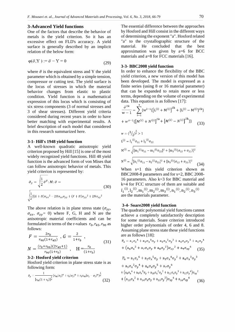
3-Advanced Yield functions One of the factors that describe the behavior of

metals is the yield criterion. So it has an

excessive effect on FLD's accuracy. A yield

surface is generally described by an implicit

relation of the below form:

(29)

where �̅� is the equivalent stress and Y the yield

parameter which is obtained by a simple tension,

compressor or cutting test. The yield surface is

the locus of stresses in which the material

behavior changes from elastic to plastic

condition. Yield function is a mathematical

expression of this locus which is consisting of

six stress components (3 of normal stresses and

3 of shear stresses). Different yield criteria

considered during recent years in order to have

better matching with experimental results. A

brief description of each model that considered

in this research summarized here.

3-1- Hill's 1948 yield function

A well-known quadratic anisotropic yield

criterion proposed by Hill [15] is one of the most

widely recognized yield functions. Hill 48 yield

function is the advanced form of von Mises that

can follow anisotropic behavior of metals. This

yield criterion is represented by:

(30)

The above relation is in plane stress state (𝜎𝑧𝑧,

𝜎𝑧𝑥, 𝜎𝑧𝑦= 0) where F, G, H and N are the

anisotropic material coefficients and can be

formulated in terms of the r-values 𝑟0, 𝑟45, 𝑟90 as

follows:

(31)

3-2- Hosford yield criterion

Hosford yield criterion in plane stress state is as

following form:

(32)

The essential difference between the approaches

by Hosford and Hill consist in the different ways

of determining the exponent "a". Hosford related

"a" to the crystallographic structure of the

material. He concluded that the best

approximation was given by a=6 for BCC

materials and a=8 for FCC materials [16].

3-3- BBC2008 yield function

In order to enhance the flexibility of the BBC

yield criterion, a new version of this model has

been developed. The model is expressed as a

finite series (using 8 or 16 material parameter)

that can be expanded to retain more or less

terms, depending on the volume of experimental

data. This equation is as follows [17]:

(33)

(34)

When s=1 this yield criterion shown as

BBC2008-8 parameters and for s=2, BBC 2008-

16 parameters. Also k=3 for BBC material and

k=4 for FCC structure of them are suitable and

𝑙1(i), l2

(i), m1(i), m2

(i), m3(i), n1

(i), n2(i), n3

(i) are the materials parameter.

3-4- Soare2008 yield function

The quadratic polynomial yield functions cannot

achieve a completely satisfactorily description

for some materials. Soare criterion introduced

higher order polynomials of order 4, 6 and 8.

Assuming plane stress state these yield functions

are as follows [18]:

(35)

(36)


(37)

In relations (32), (33) and (34), 𝑎i are material

parameters.

3-5- Plunkett2008 yield function

Plunkett et al. define CPB06 yield criterion to

describe the orthotropic metal sheet behavior. In

this criterion, anisotropy is obtained by linear

transformation of deviatory stress tensor. It can

predict tension/compression state for HCP and

FCC structural material with good accuracy.

The yield functions with two, three and four

linear transformation are shown as CPB06ex4,

CPB06ex2 and CPB06ex6 [19].

Following relation is CPB06ex2 yield function:

(38)

Where k and k' are the material parameters for

description of strength differential effects, and

"a" is the degree of homogeneity, ( Ʃ1, Ʃ2, Ʃ3)

and (Ʃ́1, Ʃ́2, Ʃ́3) are the basic value of

transformed stress tensors. The linear

transformation of deviatory stress tensor, S,

defined as follows:

(39)

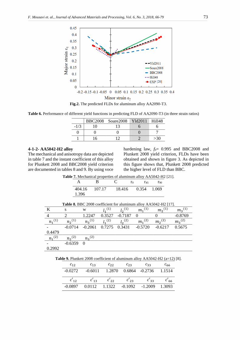
The fourth-order tensors, C and C' operating on

the stress deviator is represented by:

(40)

(41)

CPB06ex2 is used in this article named as

Plunkett 2008.

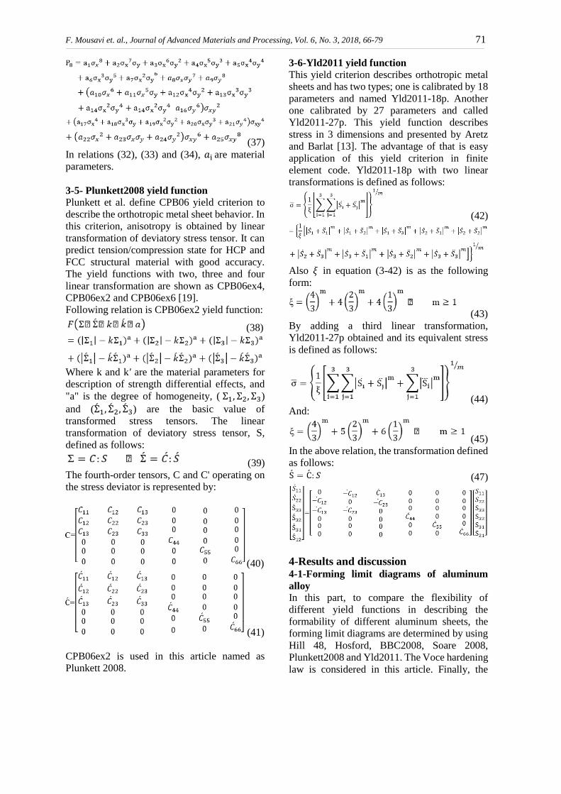
3-6-Yld2011 yield function

This yield criterion describes orthotropic metal

sheets and has two types; one is calibrated by 18

parameters and named Yld2011-18p. Another

one calibrated by 27 parameters and called

Yld2011-27p. This yield function describes

stress in 3 dimensions and presented by Aretz

and Barlat [13]. The advantage of that is easy

application of this yield criterion in finite

element code. Yld2011-18p with two linear

transformations is defined as follows:

(42)

Also 𝜉 in equation (3-42) is as the following

form:

(43)

By adding a third linear transformation,

Yld2011-27p obtained and its equivalent stress

is defined as follows:

(44)

And:

(45)

In the above relation, the transformation defined

as follows:

(47)

4-Results and discussion 4-1-Forming limit diagrams of aluminum

alloy

In this part, to compare the flexibility of

different yield functions in describing the

formability of different aluminum sheets, the

forming limit diagrams are determined by using

Hill 48, Hosford, BBC2008, Soare 2008,

Plunkett2008 and Yld2011. The Voce hardening

law is considered in this article. Finally, the


theoretical FLDs are compared to the

experimental results and the effect of yield

criteria on the prediction of the FLDs is

investigated.

4-1-1-AA2090-T3 alloy

This alloy examined in this article and forming

limit diagram is obtained by considering the

voce hardening law and the yield criteria

explained in the last part. The initial defect

factor is assumed as f0= 0.995. The mechanical

properties and anisotropy data are listed in table

1 and the parameters of yield criterions are listed

in tables 2 to 5.

Table 1. Mechanical properties of Aluminum alloy AA2090-T3 [17].

Table 2. BBC 2008 coefficient for aluminium alloy AA2090-T3 [17].

K s w 𝑙1(1)

𝑙2(1)

𝑚1(1) 𝑚2

(1) 𝑚3(1)

4 2 1.2247 0.1309 0.6217 0.7834 0.6604 0.000079

𝑛1(1) 𝑛2

(1) 𝑛3(1) 𝑙1

(2) 𝑙2

(2) 𝑚1

(2) 𝑚2(2) 𝑚3

(2)

0.111 0.0482 0.3075 1.0339 -0.0720 0.000113 0.000077 0.5380

𝑛1(2) 𝑛2

(2) 𝑛3(2)

0.0558 1.0186 0.7781

Table 3. Soare 2008 coefficient of aluminum alloy AA2090-T3 [18].

𝑎1 𝑎2 𝑎3 𝑎4 𝑎5 𝑎6 𝑎7 𝑎8

1 -1.1059 2.5255 -5.1914 6.1458 -4.3254 1.7753 14.190

𝑎9 𝑎10 𝑎11 𝑎12 𝑎13 𝑎14 𝑎15 𝑎16

-4.9759 -4.3926 3.4652 15.806 0 -9.4916 86.661 116.42

Table 5. Yld2011 coefficient of aluminum alloy AA2090-T3 (m=12) [13].

𝑐′12 𝑐′13 𝑐′21 𝑐′23 𝑐′31 𝑐′32 𝑐′44 𝑐′55 𝑐′66

0.44160 -1.18740 0.978656 1.80125 -1.7401 -0.959446 1 1

1.41126

𝑐′′12 𝑐′′13 𝑐′′21 𝑐′′23 𝑐′′31 𝑐′′32 𝑐′′44 𝑐′′55 𝑐′′66

0.7927 0.670733 0.622929 0.6655 0.962866 -0.232442 1 1 1.36

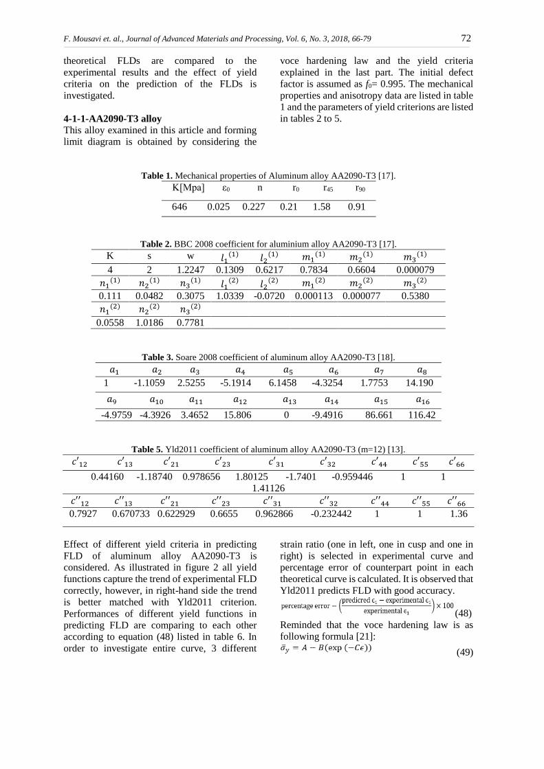
Effect of different yield criteria in predicting

FLD of aluminum alloy AA2090-T3 is

considered. As illustrated in figure 2 all yield

functions capture the trend of experimental FLD

correctly, however, in right-hand side the trend

is better matched with Yld2011 criterion.

Performances of different yield functions in

predicting FLD are comparing to each other

according to equation (48) listed in table 6. In

order to investigate entire curve, 3 different

strain ratio (one in left, one in cusp and one in

right) is selected in experimental curve and

percentage error of counterpart point in each

theoretical curve is calculated. It is observed that

Yld2011 predicts FLD with good accuracy.

(48)

Reminded that the voce hardening law is as

following formula [21]:

(49)

K[Mpa] ε0 n r0 r45 r90

646 0.025 0.227 0.21 1.58 0.91


Fig.2. The predicted FLDs for aluminum alloy AA2090-T3.

Table 6. Performance of different yield functions in predicting FLD of AA2090-T3 (in three strain ratios)

BBC2008 Soare2008 Yld2011 Hill48

-1/3 10 13 6 6

0 0 0 0 7

1 16 12 2 >30

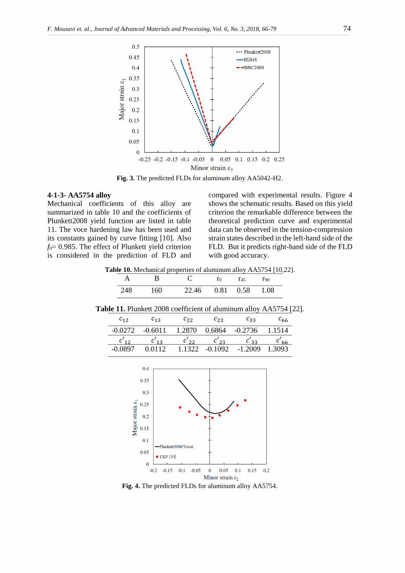
4-1-2- AA5042-H2 alloy

The mechanical and anisotropy data are depicted

in table 7 and the instant coefficient of this alloy

for Plunkett 2008 and BBC2008 yield criterion

are documented in tables 8 and 9. By using voce

hardening law, f0= 0.995 and BBC2008 and

Plunkett 2008 yield criterion, FLDs have been

obtained and shown in figure 3. As depicted in

this figure shows that, Plunkett 2008 predicted

the higher level of FLD than BBC.

Table 7. Mechanical properties of aluminum alloy AA5042-H2 [21].

A B C r0 r45 r90

404.16 107.17 18.416 0.354 1.069

1.396

Table 8. BBC 2008 coefficient for aluminum alloy AA5042-H2 [17].

K s w 𝑙1(1)

𝑙2(1)

𝑚1(1) 𝑚2

(1) 𝑚3(1)

4 2 1.2247 0.3527 -0.7187 0 0 -0.8769

𝑛1(1) 𝑛2

(1) 𝑛3(1) 𝑙1

(2) 𝑙2

(2) 𝑚1

(2) 𝑚2(2) 𝑚3

(2)

-

0.4479

-0.0714 -0.2061 0.7275 0.3431 -0.5720 -0.6217 0.5675

𝑛1(2) 𝑛2

(2) 𝑛3(2)

-

0.2992

-0.6359 0

Table 9. Plunkett 2008 coefficient of aluminum alloy AA5042-H2 (a=12) [8].

𝑐12 𝑐13 𝑐22 𝑐23 𝑐33 𝑐66

-0.0272 -0.6011 1.2870 0.6864 -0.2736 1.1514

𝑐′12 𝑐′13 𝑐′22 𝑐′23 𝑐′33 𝑐′66

-0.0897 0.0112 1.1322 -0.1092 -1.2009 1.3093


Fig. 3. The predicted FLDs for aluminum alloy AA5042-H2.

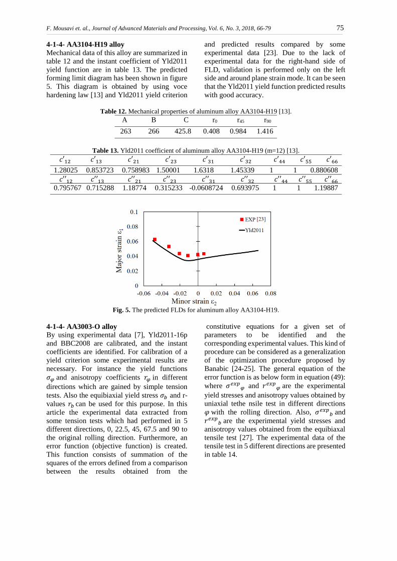
4-1-3- AA5754 alloy

Mechanical coefficients of this alloy are

summarized in table 10 and the coefficients of

Plunkett2008 yield function are listed in table

11. The voce hardening law has been used and

its constants gained by curve fitting [10]. Also

f0= 0.985. The effect of Plunkett yield criterion

is considered in the prediction of FLD and

compared with experimental results. Figure 4

shows the schematic results. Based on this yield

criterion the remarkable difference between the

theoretical prediction curve and experimental

data can be observed in the tension-compression

strain states described in the left-hand side of the

FLD. But it predicts right-hand side of the FLD

with good accuracy.

Table 10. Mechanical properties of aluminum alloy AA5754 [10,22].

A B C r0 r45 r90

248 160 22.46 0.81 0.58 1.08

Table 11. Plunkett 2008 coefficient of aluminum alloy AA5754 [22].

𝑐12 𝑐13 𝑐22 𝑐23 𝑐33 𝑐66

-0.0272 -0.6011 1.2870 0.6864 -0.2736 1.1514

𝑐′12 𝑐′13 𝑐′22 𝑐′23 𝑐′33 𝑐′66

-0.0897 0.0112 1.1322 -0.1092 -1.2009 1.3093

Fig. 4. The predicted FLDs for aluminum alloy AA5754.


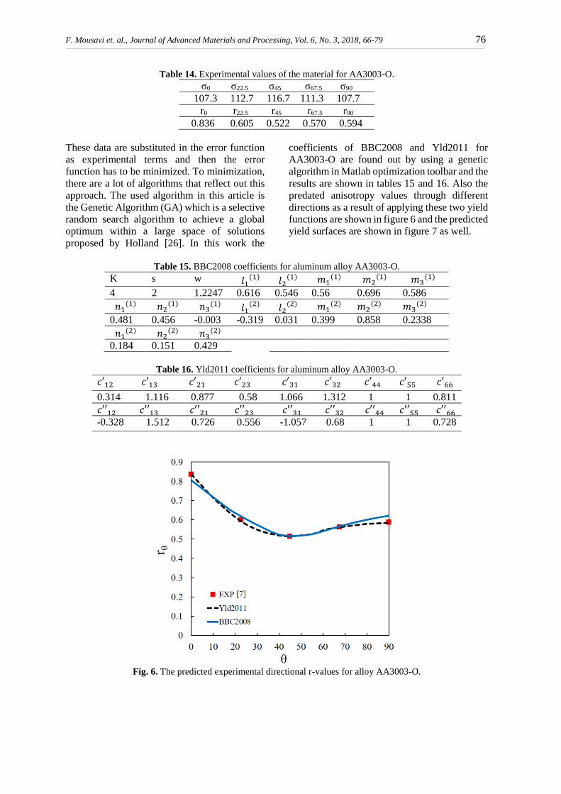
4-1-4- AA3104-H19 alloy

Mechanical data of this alloy are summarized in

table 12 and the instant coefficient of Yld2011

yield function are in table 13. The predicted

forming limit diagram has been shown in figure

5. This diagram is obtained by using voce

hardening law [13] and Yld2011 yield criterion

and predicted results compared by some

experimental data [23]. Due to the lack of

experimental data for the right-hand side of

FLD, validation is performed only on the left

side and around plane strain mode. It can be seen

that the Yld2011 yield function predicted results

with good accuracy.

Table 12. Mechanical properties of aluminum alloy AA3104-H19 [13].

A B C r0 r45 r90

263 266 425.8 0.408 0.984 1.416

Table 13. Yld2011 coefficient of aluminum alloy AA3104-H19 (m=12) [13].

𝑐′12 𝑐′13 𝑐′21 𝑐′23 𝑐′31 𝑐′32 𝑐′44 𝑐′55 𝑐′66

1.28025 0.853723 0.758983 1.50001 1.6318 1.45339 1 1 0.880608

𝑐′′12 𝑐′′13 𝑐′′21 𝑐′′23 𝑐′′31 𝑐′′32 𝑐′′44 𝑐′′55 𝑐′′66

0.795767 0.715288 1.18774 0.315233 -0.0608724 0.693975 1 1 1.19887

Fig. 5. The predicted FLDs for aluminum alloy AA3104-H19.

4-1-4- AA3003-O alloy By using experimental data [7], Yld2011-16p

and BBC2008 are calibrated, and the instant

coefficients are identified. For calibration of a

yield criterion some experimental results are

necessary. For instance the yield functions

𝜎𝜑 and anisotropy coefficients 𝑟𝜑 in different

directions which are gained by simple tension

tests. Also the equibiaxial yield stress 𝜎𝑏 and r-

values 𝑟𝑏 can be used for this purpose. In this

article the experimental data extracted from

some tension tests which had performed in 5

different directions, 0, 22.5, 45, 67.5 and 90 to

the original rolling direction. Furthermore, an

error function (objective function) is created.

This function consists of summation of the

squares of the errors defined from a comparison

between the results obtained from the

constitutive equations for a given set of

parameters to be identified and the

corresponding experimental values. This kind of

procedure can be considered as a generalization

of the optimization procedure proposed by

Banabic [24-25]. The general equation of the

error function is as below form in equation (49):

where 𝜎𝑒𝑥𝑝𝜑 and 𝑟𝑒𝑥𝑝

𝜑 are the experimental

yield stresses and anisotropy values obtained by

uniaxial tethe nsile test in different directions

𝜑 with the rolling direction. Also, 𝜎𝑒𝑥𝑝𝑏 and

𝑟𝑒𝑥𝑝𝑏 are the experimental yield stresses and

anisotropy values obtained from the equibiaxal

tensile test [27]. The experimental data of the

tensile test in 5 different directions are presented

in table 14.


Table 14. Experimental values of the material for AA3003-O.

σ0 σ22.5 σ45 σ67.5 σ90

107.3 112.7 116.7 111.3 107.7

r0 r22.5 r45 r67.5 r90

0.836 0.605 0.522 0.570 0.594

These data are substituted in the error function

as experimental terms and then the error

function has to be minimized. To minimization,

there are a lot of algorithms that reflect out this

approach. The used algorithm in this article is

the Genetic Algorithm (GA) which is a selective

random search algorithm to achieve a global

optimum within a large space of solutions

proposed by Holland [26]. In this work the

coefficients of BBC2008 and Yld2011 for

AA3003-O are found out by using a genetic

algorithm in Matlab optimization toolbar and the

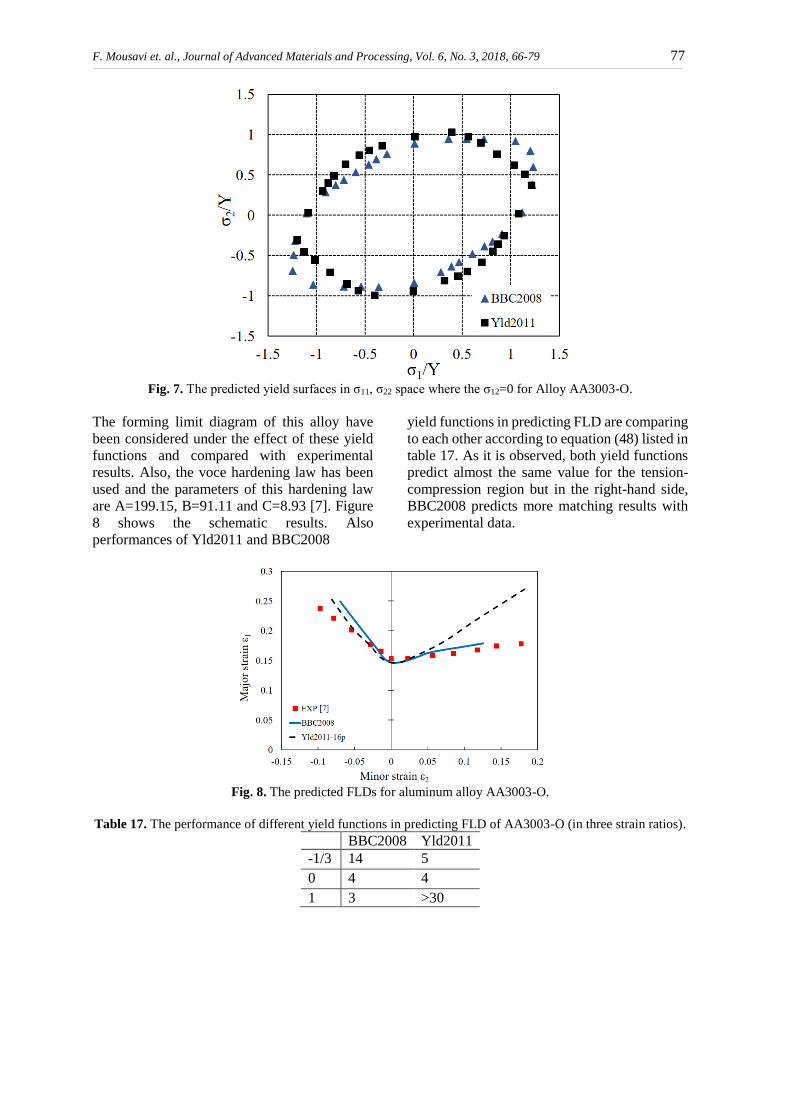
results are shown in tables 15 and 16. Also the

predated anisotropy values through different

directions as a result of applying these two yield

functions are shown in figure 6 and the predicted

yield surfaces are shown in figure 7 as well.

Table 15. BBC2008 coefficients for aluminum alloy AA3003-O.

K s w 𝑙1(1)

𝑙2(1)

𝑚1(1) 𝑚2

(1) 𝑚3(1)

4 2 1.2247 0.616 0.546 0.56 0.696 0.586

𝑛1(1) 𝑛2

(1) 𝑛3(1) 𝑙1

(2) 𝑙2

(2) 𝑚1

(2) 𝑚2(2) 𝑚3

(2)

0.481 0.456 -0.003 -0.319 0.031 0.399 0.858 0.2338

𝑛1(2) 𝑛2

(2) 𝑛3(2)

0.184 0.151 0.429

Table 16. Yld2011 coefficients for aluminum alloy AA3003-O.

𝑐′12 𝑐′13 𝑐′21 𝑐′23 𝑐′31 𝑐′32 𝑐′44 𝑐′55 𝑐′66

0.314 1.116 0.877 0.58 1.066 1.312 1 1 0.811

𝑐′′12 𝑐′′13 𝑐′′21 𝑐′′23 𝑐′′31 𝑐′′32 𝑐′′44 𝑐′′55 𝑐′′66

-0.328 1.512 0.726 0.556 -1.057 0.68 1 1 0.728

Fig. 6. The predicted experimental directional r-values for alloy AA3003-O.


Fig. 7. The predicted yield surfaces in σ11, σ22 space where the σ12=0 for Alloy AA3003-O.

The forming limit diagram of this alloy have

been considered under the effect of these yield

functions and compared with experimental

results. Also, the voce hardening law has been

used and the parameters of this hardening law

are A=199.15, B=91.11 and C=8.93 [7]. Figure

8 shows the schematic results. Also

performances of Yld2011 and BBC2008

yield functions in predicting FLD are comparing

to each other according to equation (48) listed in

table 17. As it is observed, both yield functions

predict almost the same value for the tension-

compression region but in the right-hand side,

BBC2008 predicts more matching results with

experimental data.

Fig. 8. The predicted FLDs for aluminum alloy AA3003-O.

Table 17. The performance of different yield functions in predicting FLD of AA3003-O (in three strain ratios).

BBC2008 Yld2011

-1/3 14 5

0 4 4

1 3 >30


5- Conclusion

In this paper, the effect of various developed

yield functions were applied to consider the

anisotropy of aluminum alloys and to find out

their capabilities in predicting anisotropy of

metals. Forming limit diagrams of these alloy

generated refer to the M-K model and the results

were compared with experimental ones.

Forming limit diagrams for AA5754,

AA3104-H19, AA5042 and AA2090

are gained by different yield criteria

such as BBC2008, Punkett2008,

soare2008 and Yld2011 using available

coefficients of these yield functions in

literatures [8,13,17,22] and voce

hardening law.

Comparing the results according to

these developed yield functions for

aluminum alloy 2090-T3 shows that all

advanced yield functions correctly

anticipate the overall trend but in the left

side of the curve, predicted results by

Yld2011 are better matched with

experimental data.

Forming limit of AA5754 is obtained

based on Plunkett yield criterion. The

remarkable difference between the

theoretical prediction curve and

experimental data can be observed in

the tension-compression strain states

described in the left-hand side of the

FLD, but it predicts right-hand side of

the FLD with good accuracy.

Analyzing the FLDs for AA5042-H2

which gained by using Plunkett2008

and BBC2008 shows that, Plunkett

2008 predicted the higher level of FLD

than BBC.

For AA3003-O coefficients of

BBC2008 and Yld2011 are found out

using minimization of error function

through genetic algorithm in Matlab

optimization toolbar. Conformity of

predicted directional r-values with

experimental ones affirm the accuracy

of them.

Forming limit diagram of AA3003-O

are predicted by BBC2008 and Yld2011

and compared with experimental data.

Both yield functions predict almost the

same value for tension-compression

region but in right-hand side, BBC2008

predicts results with better accuracy.

References

[1] A. Assempour, R. Hashemi, K. Abrinia, M.

Ganjiani, E. Masoumi, “A methodology for

prediction of forming limit stress diagrams

considering the strain path effect”,

Computational materials science, vol. 45, no. 2,

pp. 195-204, 2009.

[2] A. Assempour, A.R. Safikhani, R. Hashemi,

“An improved strain gradient approach for

determination of deformation localization and

forming limit diagrams”, Journal of Materials

Processing Technology, vol. 209, no. 4, pp.

1758-1769, 2009.

[3]Z. Marciniak and K. Kuczynski, “Limit

strains in the processes of stretch-forming sheet

metal,” International journal of mechanical

sciences, vol. 9, no. 9, pp. 609IN1613–

612IN2620, 1967.

[4] R. Hashemi, K. Abrinia, “Analysis of the

extended stress-based forming limit curve

considering the effects of strain path and

through-thickness normal stress”, Materials and

Design, vol. 54, pp. 670-677, 2014.

[5] M. Butuc, D. Banabic, A. B. da Rocha, J.

Gracio, J. F. Duarte, P. Jurco, and D. Comsa,

“The performance of yld96 and bbc2000 yield

functions in forming limit prediction,” Journal

of materials processing technology, vol. 125, pp.

281–286, 2002.

[6] M. Ganjiani and A. Assempour, “An

improved analytical approach for determination

of forming limit diagrams considering the

effects of yield functions,” Journal of materials

processing technology, vol. 182, no. 1,pp. 598–

607, 2007.

[7] S. Ahmadi, A. Eivani, and A. Akbarzadeh,

“An experimental and theoretical study on the

prediction of forming limit diagrams using new

bbc yield criteria and m–k analysis,”

Computational Materials Science, vol. 44, no. 4,

pp. 1272–1280, 2009.

[8] J.-H. Yoon, O. Cazacu, J. W. Yoon, and R.

E. Dick, “Earing predictions for strongly

textured aluminum sheets,” International journal

of mechanical sciences, vol. 52, no. 12, pp.

1563–1578, 2010.

[9] A. Rezaee-Bazzaz, H. Noori, and R.

Mahmudi, “Calculation of forming limit

diagrams using hill’s 1993 yield criterion,”


International Journal of Mechanical Sciences,

vol. 53, no. 4, pp. 262–270, 2011.

[10]P. Dasappa, K. Inal, and R. Mishra, “The

effects of anisotropic yield functions and their

material parameters on prediction of forming

limit diagrams,” International Journal of Solids

and Structures, vol. 49, no. 25, pp. 3528–3550,

2012.

[11] X. Li, N. Song, G. Guo, and Z. Sun,

“Prediction of forming limit curve (flc) for al–li

alloy 2198-t3 sheet using different yield

functions,” Chinese Journal of Aeronautics, vol.

26, no. 5, pp. 1317–1323, 2013.

[12] S. Panich, F. Barlat, V. Uthaisangsuk, S.

Suranuntchai, and S. Jirathearanat,

“Experimental and theoretical formability

analysis using strain and stress based forming

limit diagram for advanced high strength steels,”

Materials & Design, vol. 51, pp. 756–766, 2013.

[13] H. Aretz and F. Barlat, “New convex yield

functions for orthotropic metal plasticity,”

International Journal of non-linear mechanics,

vol. 51, pp. 97–111, 2013.

[14] S. Panich and V. Uthaisangsuk, “Effects of

anisotropic yield functions on prediction of

forming limit diagram for ahs steel,” in Key

Engineering Materials, vol. 622. Trans Tech

Publ, 2014, pp. 257–264.

[15] R. Hill, “A theory of the yielding and plastic

flow of anisotropic metals,” in Proceedings of

the Royal Society of London A: Mathematical,

Physical and Engineering Sciences, vol. 193, no.

1033. The Royal

Society, 1948, pp. 281–297.

[16] R. W. Logan and W. F. Hosford, “Upper-

bound anisotropic yield locus calculations

assuming¡ 111¿-pencil glide,” International

Journal of Mechanical Sciences, vol. 22, no. 7,

pp. 419–430, 1980.

[17] D.-S. Comsa and D. Banabic, “Plane-stress

yield criterion for highly-anisotropic sheet

metals,” Numisheet 2008, Interlaken,

Switzerland, pp.43–48, 2008.

[18] S. Soare, J. W. Yoon, and O. Cazacu, “On

the use of homogeneous polynomials to develop

anisotropic yield functions with applications to

sheet forming,” International Journal of

Plasticity, vol. 24, no. 6, pp.

915–944, 2008.

[19] B. Plunkett, O. Cazacu, and F. Barlat,

“Orthotropic yield criteria for description of the

anisotropy in tension and compression of sheet

metals,” International Journal of Plasticity, vol.

24, no. 5, pp. 847–866, 2008.

[20] R. Zhang, Sh. Zhutao, L. Jianguo, “A

review on modelling techniques for formability

prediction of sheet metal forming,” International

Journal of Lightweight Materials and

Manufacture, 2018.

[21] E. Voce, “The relationship between stress

and strain for homogeneous deformation,” J Inst

Met, vol. 74, pp. 537–562, 1948.

[22] K. Inal, R. K. Mishra, and O. Cazacu,

“Forming simulation of aluminum sheets using

an anisotropic yield function coupled with

crystal plasticity theory,” International Journal

of Solids and Structures, vol. 47, no. 17, pp.

2223–2233, 2010.

[23] S. Soare and D. Banabic, “A note on the mk

computational model for predicting the forming

limit strains,” International Journal of Material

Forming, vol. 1, no. 1, pp. 281–284, 2008.

[24] D. Banabic, O. Cazacu, F. Barlat, D.

Comsa, S. Wagner, and K. Siegert, “Description

of anisotropic behaviour of aa3103-0 aluminium

alloy using two recent yield criteria,” in Journal

de Physique IV (Proceedings), vol. 105. EDP

sciences, 2003, pp. 297–304.

[25] D. Banabic, H. Aretz, D. Comsa, and L.

Paraianu, “An improved analytical description

of orthotropy in metallic sheets,” International

Journal of Plasticity, vol. 21, no. 3, pp. 493–512,

2005.

[26] J. H. Holland, Adaptation in natural and

artificial systems: an introductory analysis with

applications to biology, control, and artificial

intelligence. U Michigan Press, 1975.

[27] R. Safdarian, “Forming limit diagram

prediction of 6061 aluminum by GTN damage

model,” Mechanics & Industry, Vol. 19, Issue 2,

pp. 202-214, 2018.

Documents

Effect of Different Yield Functions on Computations of