Embed Size (px)
Citation preview

1
MATLAB, short for MATrix LABoratory, is a multi-purpose application developed by
the MathWorks, Inc. It provides a single platform for computation, visualization,
programming and software development. The MATLAB family of programs consists
of the main program, namely, MATLAB, and add-on toolboxes, which extend the
functionality of MATLAB. MATLAB is available in the School of Engineering and
Applied Science (SEAS) on the PC-platform. As of this writing, the following
toolboxes are supported:
� Simulink � Signal processing � Communications
� DSP blockset � Image processing � Fuzzy logic
� Neural networks � Control � Optimization
� Data acquisition � Wavelets � Real-time workshop
� Symbolic math � Statistics � Stateflow
� MATLAB compiler
MATLAB Environment

2
How to get started?
Locate the MATLAB program icon on the desktop of your computer and double click
it to launch the program. This action opens the Command window, showing the
prompt on the left corner (>>or EDU>>). Once MATLAB has been started, the
program interpreter is ready to execute MATLAB commands.
This is the workspace
which lists all the
variables you are using
This is the command
history window, it
displays a log of the
commands used
You may type the
commands after
the MATLAB
prompt “ >>”
This is the COMMAND
WINDOW, you can
enter commands and
data, and the results
are displayed here.
This is the directory that
MATLAB will look at for all
the files, make sure it is set
to the right folder
A session may be terminated by simply typing quit or exit at the MATLAB prompt,
followed by the “enter” key, i.e.,
>>quit <enter>

3
- The most basic way to get started : BASIC COMPUTATION-
MATLAB can be used as an expression evaluator. You simply enter the expression
much like a high powered hand calculator without specifying variables. Command
lines are evaluated as soon as they have been concluded by pressing the Enter key.
Let’s start with some simple math. In the MATLAB command window type in the
following expression:
Example
- Execute a computation by pressing Enter -
>>7/3 <enter>
To which MATLAB responds with
ans =
2.3333
Since no variable was defined, MATLAB assigns the result to the generic variable
called “ans” that stands for “answer”. Try the following examples:
Practice
- “ans” stands for “answer”-
>>12.5*(11.63+9.72)/3.3 <enter>
>>1+sin(pi/3)/(2+cos(pi/12)) <enter>
>>sqrt(1+tan(pi/12)/(1+sin(pi/2))) <enter>
>>2^(log2(8)) <enter>
Format Command
- “format” and “format long” Command
All computations in MATLAB are done in double precision (8 bytes to represent a
number). However, the screen output can be displayed in several formats. The
command format provides control over the display of the answers. short format, the
default, displays numerical data with four digits after the decimal point. While long
format display fourteen digits.

4
Example
- The “format” command-
>>format long <enter> → changes a current format to the format long
>>7/3 <enter>
MATLAB returns
ans =
2.33333333333333
The single command format will revert the display back to default. You simply need
to enter “format” and press “enter”:
>>format <enter>
The Primary Mathematical Operators
In MATLAB, the standard arithmetic operations are denoted as follows:
SYMBOL MEANING
+ Addition
- Subtraction
* Multiplication
/ Division
^ Exponentiation
MATLAB Variables
Like most programming languages, MATLAB allows you to create variables, and
assign values to them. Variables can represent “scalars”, “vectors”, “matrices”, or
“strings”. Variables in MATLAB can have any names except reserved names used

5
for MATLAB functions, so you would not want to name a variable “mean” or “std”-
the program will not allow this. It is a good practice to use variable names that
describe the quantity they represent. The names of variables should begin with a
letter but may be followed by any combination of letters, digits or underscores (don’t
use space). MATLAB recognizes only the first 31 characters of a variable name.
Thus, xab, x12c, and x12_c are all legal names. MATLAB variables are created when
they appear on the left of an equal sign. The generic statement “variable=expression”
creates the “variable” and assigns to it the value of the “expression” on the right hand
side.
Real scalars may be entered by a simple assignment of the form,
>>total=9+11;
The statement above will cause the expression to the right of “=” to be evaluated. The
result (in this case 20) is stored in the variable total.
��NOTE��
All variables used in the current MATLAB session are saved in the Workspace. Once
you exit MATLAB, all values of the variable are lost.
Usage of Semicolon
Looking at the example above, the semicolon at the end of the statement has the effect
of suppressing the output, so that nothing is printed on the screen. Without the
semicolon, the result will be printed out immediately. In fact, when a statement is
followed by a semicolon (;), the statement is executed, but the result is just not printed
in the command window. The value of any variable is printed by simply typing its
name, and hitting <enter>. Thus,
>>total <enter>
results in
total =
20

6
What Are Strings?
So far, all the variables we have dealt with assume numerical values, but it is often
useful to be able to manipulate other types of data. Strings are the form of data used
in programming languages for storing and manipulating text, such as words, names,
and sentences. An example of a string is,
>>s=’Too much of any one thing becomes drudgery’
Strings in MATLAB
The single quotation marks are not part of the string. They are there to mark off the
string. In MATLAB, string constants are surrounded by single quotation marks; this
is how MATLAB recognizes a string. To insert an apostrophe inside a string, a
double apostrophe must be used. Strings can be assigned to a variable just like a
number, as long as the text is put within single quotes.
>>firstname=’Valerie’;
>>lastname=’Mollo’;
Strings can be joined together just like two vectors could, though it looks nicer to put a
space between using ‘ ‘.
>>fullname=[firstname,’ ‘,lastname]
‘Valerie Mollo’
>>age=37;
>>agestring=[fullname,’ is ’,num2str(age),’ years old ’]
String Command
- “strcmp and findstr”
MATLAB has a set of string manipulation functions, namely, strcmp and findstr.
The first one is a logical operator.

7
� Syntax
MATLAB also offers other string commands:
The functions num2str and int2str will convert a numeric variable to its string
representation. This is particularly useful for including values of a parameter in either
title or axes labels.
COMMAND MEANING
int2str(a) Turn the integer ‘a’ into a character string
num2str(a) Turn the number “a” into a string
str2num(s) Turn a string “s” into a number
str2mat Groups different strings into a matrix
Strcmp Findstr
>> strcmp (x,y) >>findstr (x,y)
returns a value of 1 if the strings x and y
are identical; otherwise it returns a value
of zero
finds the first occurrence of string x
within string y
Practice
-String Command-
>>x=’Programming with MATLAB is fun’;
>>y=’Programming with MATLAB is simple’;
>>strcmp(x,y)
ans =
0
>>findstr(x,’u’)
ans =
29

8
Case Sensitivity
- and the “casesen” command
As in C programming language, MATLAB is case (upper and lower case) sensitive
(upper and lowercase letters are not interchangeable). In other words, student,
Student, and STUDENT are three distinct variables. If this proves to be an
annoyance, the command casesen will toggle the case sensitivity off and on. It is
useful to keep all your writing in lower case to avoid errors associated with case
sensitivity.
Precedence of Operators
All operators in MATLAB are ranked according to their precedence. Exponentiation
has the highest precedence, followed by multiplication and division, and finally
addition and subtraction. Operations are evaluated from left to right. Parenthesis
can be used to over-ride these usual rules of precedence.
Precedence Ranking
1. Exponentiation
2. Multiplication & Division
3. Addition and Subtraction
Comments
Every computer language provides a facility for documenting a program. This
optional facility lets you describe statements in the source program to make it clear to
the reader what is going on. Your code must be commented and it should be written
in such a way as if someone else is going to have to understand the program without
your help. Include comments that clearly explain the logic of what you are doing.
There are several ways to include comments. Any statement that begins with a
percentage sign (%) is considered to be a comment and ignored by MATLAB.
Comments could either start at the beginning or anywhere in a line. Here is an
example:
>>% This line is a comment

9
Second, you can add a comment to the end of a statement by prefacing the comment
with a percentage sign (%). Here is an example:
>> [z,p,k]=buttap(4); % Here is a comment
Elementary Mathematical Functions
MATLAB has a very large library of built-in functions for mathematical and scientific
computations. Here is a summary of some relevant functions.
A. Trigonometric
Symbol Meaning Symbol Meaning
sin - Sine sec - Secant
sinh - Hyperbolic sine sech - Hyperbolic secant
asin - Inverse sine asec - Inverse secant
asinh - Inverse hyperbolic sine asech - Inverse hyperbolic secant
cos - Cosine csc - Cosecant
cosh - Hyperbolic cosine csch - Hyperbolic cosecant
acos - Inverse cosine acsc - Inverse cosecant
acosh - Inverse hyperbolic cosine acsch - Inverse hyperbolic cosecant
tan - Tangent cot - Cotangent
tanh - Hyperbolic tangent coth - Hyperbolic cotangent
atan - Inverse tangent acot - Inverse cotangent
atan2 - Four quadrant inverse tangent acoth - Inverse hyperbolic cotangent
atanh - Inverse hyperbolic tangent

10
B. Exponential
Symbol Meaning
exp
log
log10
log2
pow2
sqrt
nextpow2
- Exponential
- Natural logarithm
- Common (base 10)
- Base 2 logarithm and dissect floating point number
- Base 2 power and scale floating point number
- Square root
- Next higher power of 2
C. Additional Math Functions
Symbol Meaning
square(x)
sawtooth(x)
sign(x)
rem(x,y)
sinc(x)
erf(x)
erfc(x)
erfinv(x)
- Generate a square wave with period 2π
- Generate a sawtooth wave with period 2π
- Signum function of x
- Remainder when x is divided by y
- sin(πx)/ πx
- Error function of x
- Complementary error function of x
- Inverse Error function of x
Predefined Variables
Predefined Variables MEANING
pi π (ratio of circumference to diameter of a circle 22/7 )
Inf ∞
Not-a-Number,e.g.,
0, ,0
∞−∞+∞
∞
NaN (obtained as a result of the mathematically undefined
operations, such as, 0
0, or ∞−∞ )
i,j 1−
nargin Number of function input arguments used
margout Number of function output arguments used
eps Floating point precision

11
��NOTE��
Special variables can be assigned any value but when MATLAB is restarted or after
execution of clear command, the original values are restored.
Practice
-Build-in Functions & Predefined Variables-
(1)
Use MATLAB to evaluate the following expressions:
1. (7+3)=5 <enter>
2. (9-5)*6 <enter>
3. 3*cos(3*pi/4) <enter>
4. 3^2 <enter>
5. sqrt(5) <enter>
6. exp(5) <enter>
7. log(exp(2)) <enter>
8. 15/2 <enter>
9. 2\15 <enter>
10. atan(pi/4) <enter>
11. log10(100) <enter>
12. 3+sqrt(7) <enter>
Practice
-Build-in Functions & Predefined Variables-
(2)
Evaluate the following expression:
3 5c rA B− −
>>c=2.3; r=5.1; A=3.4; B=1.5;
>>c^3-sqrt(r*A)-5*B <enter>
12
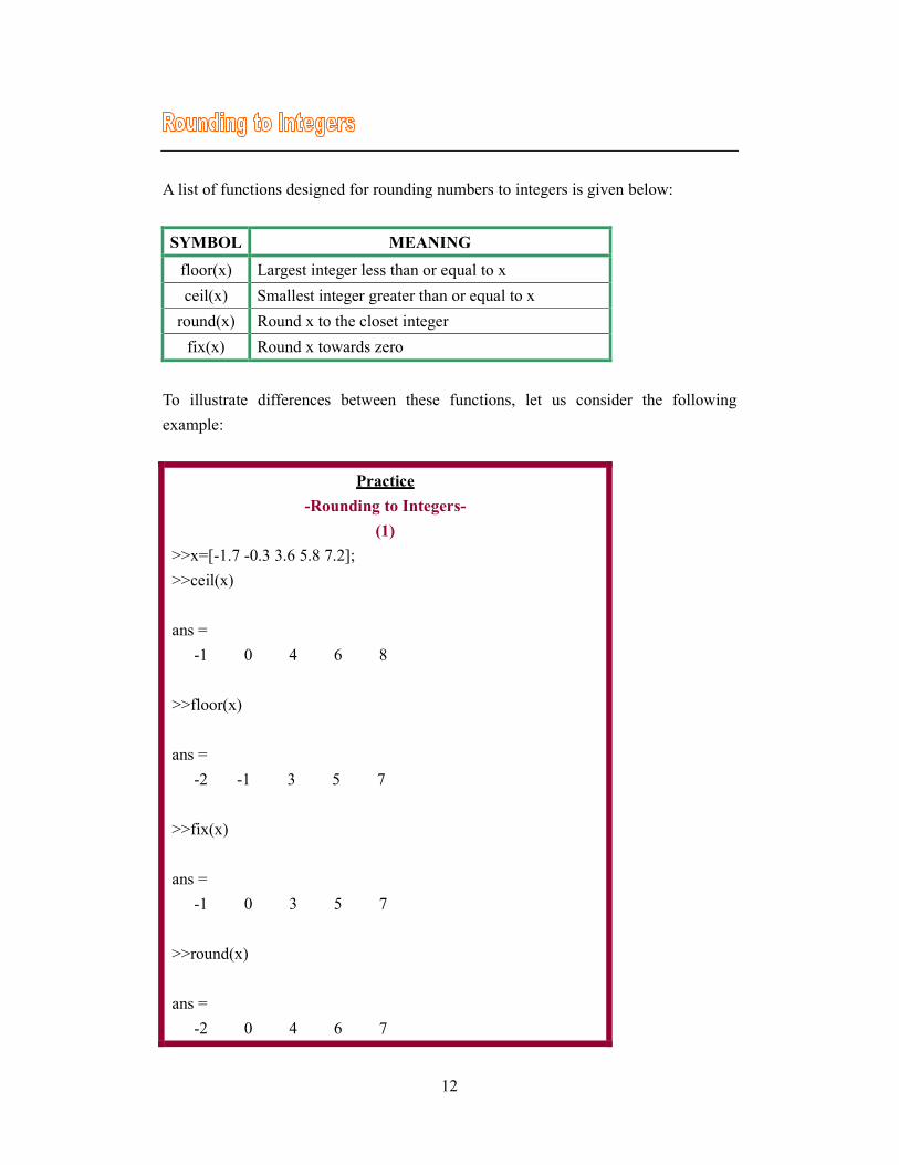
A list of functions designed for rounding numbers to integers is given below:
SYMBOL MEANING
floor(x) Largest integer less than or equal to x
ceil(x) Smallest integer greater than or equal to x
round(x) Round x to the closet integer
fix(x) Round x towards zero
To illustrate differences between these functions, let us consider the following
example:
Practice
-Rounding to Integers-
(1)
>>x=[-1.7 -0.3 3.6 5.8 7.2];
>>ceil(x)
ans =
-1 0 4 6 8
>>floor(x)
ans =
-2 -1 3 5 7
>>fix(x)
ans =
-1 0 3 5 7
>>round(x)
ans =
-2 0 4 6 7

13
Practice
-Rounding to Integers-
(2)
1. What is the integer closest to 173 ?
>>x=sqrt(173); <enter>
>>round(x) <enter>
2. Between what consecutive integers does ( )52 1π + lie?
>>x=(pi^2+1)^5; <enter>
>>lbound=floor(x) <enter>
>>ubound=ceil(x) <enter>
answer: lbound<x<ubound
It is often the case in computer engineering to convert numbers from one base to
another. MATLAB has a number of functions tailored for that purpose. These
functions are bin3dec, dec2bin, hex2dec, dec2hex, dec2base, and oct2dec. Table
below provides a summary of these functions.
Function Meaning
dec2bin Convert decimal to a binary string
bin2dec Convert binary string to decimal integer
dec2hex Convert decimal to hexadecimal
hex2dec Convert hexadecimal to decimal
dec2base Convert dec numbers to octal numbers
oct2dec
hex2bin
Convert octal numbers to decimal numbers
Convert hexadecimal strings to binary strings

14
Practice
-Base Conversions-
Make the following base conversions:
1. ( )8
723542 to decimal
>>oct2dec(723542)
ans: 239458
3. ( )16
4 52E B to binary
>>dec2bin(hexdec(‘4E52B’)
ans: 1342453
5. ( )2
1001011 to decimal
>>bin2dec(‘1001011’)
ans: 75
2. ( )10
8451 to binary
>>dec2bin(8451)
ans:10000100000011
4. ( )16
5 52C B to octal
>>dec2base(hex2dec(‘5C52B’),8)
ans =1342453
-Commands You Have to Know-
Basic commands
The who command lists all the variables currently in workspace, and the whos
command list the variables in workspace and gives extra information regarding
memory allocation, class of the variables in memory, and size in bytes. Entering the
clear command without arguments removes all the variables in the current workspace
and clear followed by the name of any variable deletes only that variable in workspace
leaving other ones intact. The clc command clears the command window and resets
the command prompt at the top of the screen.

15
Practice
-Commands & Help-
(1)
>> x=1;
>> y=3;
>> d=[1 2; 4 5];
>> whos
Name Size Bytes Class
ans 1x5 40 double array
d 2x2 32 double array
x 1x1 8 double array
y 1x1 8 double array
Grand total is 11 elements using 88 bytes
Practice
-Commands & Help-
(2)
1. Use MATLAB to find the area of a circle of radius equal to 3.5.
>>%Evaluation of the area of a circle
>>radius=3.5; <enter> % set radius to 3.5
>>area=pi*r^2 <enter> % compute the area of the circle
2. Create three variables x, y, and z, then use the who, and whos commands to display
the variables in workspace. Afterwards clear all the variables and the MATLAB
command window.
>>x=2*cos(pi/6); <enter> % define variable x
>>y=5*sin(pi/4); <enter> % define variable y
>>z=exp(pi*sqrt(23)) <enter> % define variable z
>>who <enter> % display the list of variables in workspace
>> whos<enter> % give the list of variables with additional attributes
>>clear x <enter> % clear variable x
>>clear <enter> % clear all remaining variables
>>clc <enter> % clear command line window
16
��NOTE��
If a statement does not fit in the 80 spaces available on a line, you can split it over two
(or more) lines by placing an ellipsis (three periods) at the end of the line and resume
typing on the next line.
>>x=sin(2*pi*3*t)+2*sin(2*pi*6*t)+7*sin(2*pi*9*t)+…
3*sin(2*pi*12*t);
On-screen Help
One of the nice features of MATLAB is its help system. There are many sources of
help in MATLAB. During any MATLAB session, online help is available for a
variety of topics. If you know the name of the command you want help on, you can
use the MATLAB help command followed by the name of the command to determine
its syntax.
>>help command name <enter>
>>help sin <enter> % provide the syntax for the sine function
A. “lookfor” Command
If you are unsure about the spelling or existence of a command, you can try to find it
using the lookfor command. The lookfor command searches the MATLAB files and
returns the names containing a specific keyword.
>>lookfor hilbert <enter> % retrieve all commands containing the keyword Hilbert
B. “help” Command
As soon as the command name is found, use the help command to retrieve its syntax.
If you type help with no parameters a list of main MATLAB topics appear on the
screen, while help topic_name returns all available commands on the specified topic.
>>help <enter> % return a list of the main MATLAB topics
>>help signal <enter> % return a list of functions of the signal processing toolbox

17
Row Vector
A straightforward way to generate a row vector is to list its elements, surrounded by
square brackets [ ]. Either commas or blanks may separate the elements of a vector.
For example, to create a vector having as elements 3,5,7,9, and 11, just enter:
>>x=[3 5 7 9 11] <enter> % define a row vector
MATLAB should return
x =
3 5 7 9 11
Column Vector
Column vectors have similar constructs to row vectors, but semicolons separate the
entries.
>>x=[3; 5; 7; 9; 11] <enter> % define a column vector
Row Vector → Column Vector
It is possible to turn a row vector into a column vector (and vice versa) via a process
called transposing and defined using the prime operator (apostrophe), [‘].
>>x=[3 5 7 9 11]; <enter> % specify a row vector
>>x’ <enter> % convert a row vector into a column vector
Evenly Spaced Vectors
This way of defining vectors becomes awkward for large data sets (this can be time
consuming), moreover, common vectors are those of equally spaced numbers.
MATLAB provides a more flexible way of constructing vectors of evenly spaced
values over a given range. The colon operator [:] is used for this purpose. The colon
will be used most often to generate vectors for creating x-y plots. The general form of

18
the statement is:
>>x=start:step:end;
where start and end are the lower and upper bounds of the interval and step
(increment) is the step size.
Practice
-Evenly Spaced Vector-
(1)
x=0:0.1:1 <enter> % generate 11 data pts from 0 through 1 in increments of 0.1
x = Columns 1 through 9
0 0.1000 0.2000 0.3000 0.4000 0.5000 0.6000 0.7000
0.8000
Columns 10 through 11
0.9000 1.0000
You can reference individual items within the vector. To change the sixth element
in the x vector, proceed as follows:
>>x(6)=0.45
��NOTE��
It is just as easy to use negative increments.
>>x=7:-1;2 <enter> % generate an array with negative step size
If the step size is omitted, a value of 1 is used.
>>x=0:5 <enter> % generate an array with step size of 1

19
Practice
- Even Increment-
(2)
Compute the sum of the finite geometric series
21 ... ns r r r= + + + +
Where the common ratio is r=0.6 and n=10.
>>n=0:10;
>>r=0.6;
>>s=sum(r.*n) <enter>
%define the running index n
% specify the ratio of the geometric series
% evaluate the partial sum
Practice
-Even Increment-
(3)
We are given a vector x=[0:0.2:3].
1. Determine the seventh component of x
2. Determine the length of x
>>x=[0:0.2:3]; % specify vector x
>>x(7) % specify the seventh component of x
>>length (x) <enter> % return the length of the vector x
��NOTE��
In MATLAB, all arrays are indexed starting with 1, i.e., x(1) is the first element of the
array x. The notation x(1:12) means the first 12 elements of the vector x.
Length vs. size: The length of a vector is the number of values it holds. The size of a
vector is the number of rows by the number of columns.

20
Product of Vectors
Practice
-Product of Vectors-
Compute the dot product of the following vectors:
>>x=[1 2 3];
>>y=[4 5 6];
>>x*y’ <enter>
Commands for Generating Vectors
- linspace & logspace
A. “linspace” Command
MATLAB has two built-in functions to generate vectors. The linspace function
creates linearly spaced vectors of length n over the range from start to end (if the
length is omitted, MATLAB assumes 100 points). The command structure is as
follows:
>>x=linspace (start,end,n);
Practice
-“linspace” Command-
Write a piece of code to convert temperatures from degrees Fahrenheit to degrees
centigrade.
>>F=linspace(0,9,10); <enter> % specify evenly spaced temperatures
>>C=(F-32)*5/9; <enter> % Fahrenheit to Centigrade conversion
>>[F’ C’] <enter> % display both temperatures as column vectors
ans =
0 -17.7778
1.0000 -17.2222
2.0000 -16.6667
3.0000 -16.1111
4.0000 -15.5556
5.0000 -15.0000
6.0000 -14.4444
7.0000 -13.8889
8.0000 -13.3333
9.0000 -12.7778

21
B. “logspace” Command
The function logspace generates a logarithmically spaced vector of length n ranging
from 10start to 10end . The command structure is as follows:
>>x=logspace(start,end,n)
>>x=logspace(0,2,5) <enter> % create a vector of length 5 ranging from 1 to 100
Term-by-term Operations
MATLAB has special operators, to carry out term-by-term multiplication, division,
and exponentiation. An operator preceded by a dot (or period) causes the operation to
be performed term-by-term. These operators are shown in the following table:
SYMBOL TERM-BY-TERM OPERATION
.* Multiplication
./ Division
.^ Exponentiation
Suppose that we have the vectors
[ ]1 2, ,..., nx x x x= and
[ ]1 2, ,..., ny y y y= . Then
x.*y=[ ]1 1 2 2, ,..., n nx y x y x y
x./y= 1 2
1 2
, ,..., n
n
xx x
y y y
x.^p=1 2, ,...,p p p
nx x x

22
Practice
- Term-by-term Operations-
(1)
>>% Term-by-term multiplication
>>x=[1 2 3]; % specify vector x
>>y=[2 4 1]; % specify vector y
>>z=x.*y <enter> % compute the term by term product
>>%Term-by-term division
>>x=[1 2 3] % specify vector x
>>y=[2 4 1]; % specify vector y
>>z=x./y <enter> % compute the term by term division
>>%Term-by-term exponentiation
>>x=[1 2 3]; % specify vector x
>>y=[2 4 1]; % specify vector y
>>z=x.^y <enter> % compute the term by term
exponentiation
Practice
- Term-by-term Operations -
(2)
A supermarket conveyor belt holds an array of groceries.
Product Quantity Unit Price Sub_total
A 4 1.5 4 x 1.5
B 3 0.5 3 x 0.5
C 2 2.5 2 x 2.5
D 5 0.95 5 x 0.95
Total 17.25
The prices of each product (in pounds) are [1.5 0.5 2.5 0.95]; while quantities of
each product are [4 3 2 5]. Use MATLAB to calculate the total bill.
>> price=[1.5 0.5 2.5 0.95];
>> quantity=[4 3 2 5];
>> sub_total= price.*quantity
>> total= sum(sub_total)

23
- Complex Arithmetic & Algebra
MATLAB can handle both real as well as complex data. In this section, we shall
explore the use of MATLAB for doing complex arithmetic and algebra.
Usage of Variable i or j
The number, 1− , is identified in MATLAB by the variables i or j. Using j (i is
typically dedicated to electrical current), one can generate complex numbers.
Therefore, a complex number, such as z=3+5j, may be input as z=3+7j or z=3+7*j.
MATLAB always displays the imaginary unit as i.
Practice
- Usage of variable i or j-
>>z=2+3j; % define a complex number z
Commands for Complex Numbers
A. real(z) & imag(z)
MATLAB provides several built-in functions to work with complex numbers. We can
extract the real and imaginary parts of an arbitrary complex number by the functions
real(z) and imag(z).
Practice
-Commands: real(z) & imag(z)-
>>z=3+5j; <enter> % define a complex number z
>>x=real(z) <enter> % extract the real part of z and store the result in x
>>y=imag(z) <enter> % extract the imaginary part of z and store the result in y
B. abs(z), angle(z) & conj(z)
To convert to polar notation, the function abs(z) and angle(z) ( )( )angle zπ π− < ≤ ,

24
compute the modulus (magnitude) of the complex number and its phase in radians,
respectively. Lastly, conj(z) returns the complex conjugate of the complex number z.
Practice
-Commands: abs(z), angle(z) & conj(z)-
>>z=5+3j; % define a complex number z
>>mag=abs(z) <enter> % compute the magnitude of z
>>phase=angle(z) <enter> % compute the phase in radians
>>phase=angle(z)*180/pi <enter> % compute the phase in degrees
>>zbar=conj(z) <enter> % compute the complex conjugate of z
Summary of basic functions for manipulating complex numbers, where z is a complex
number:
Matlab Command Meaning
real(z)
imag(z)
abs(z)
angle(z)
conj(z)
Re(z)
Im(z)
|z|
∢ z
z*
C. “cart2pol” & “pol2cart” Command
It is often the case to convert a complex number from a Cartesian form to polar form
and vice versa. MATLAB has built-in functions cart2pol and pol2cart that perform
conversion from Cartesian to polar and polar to Cartesian, respectively.
Function Synopsis
>>z1=x+j*y; % define a complex number in Cartesian form
>>z2=mag*exp(j*theta); % define a complex number in polar form
>>[theta, mag]=cart2pol(x,y); % conversion from Cartesian to polar
>>[x,y]=pol2cart(theta, mag); % conversion from polar to Cartesian

25
Practice
-“cart2pol” Command-
Express the given complex number in polar form
>> z=-2+0.5j; % define a complex number in Cartesian form
>>[theta, mag]=cart2pol(-2,0.5) % provide polar form of z
theta =
2.8966
mag =
2.0616
2.89662 0.5 2.061 jz j e∴ = − + =
Practice
-Complex Numbers-
(1)
1. Use MATLAB to evaluate the magnitude and phase of the given complex
numbers.
>>z1=2+3j;
>>z2=2+j;
>>z3=-2-3j;
>>z4=1-3j;
2. Express the numbers defined in part (1) in polar form
3. Determine z1*z2, and z1/z2
4. Determine z3+z4, and z4-z3
5. Determine the real part of 2 2( 1) ( 2)z z×
6. Determine the imaginary part of 4 3( 1) /( 2)z z
Plot z1 using plot(z1,’x’). This command will plot the imaginary part versus the
real part.

26
Practice
-Complex Numbers-
(2)
Check the following identities:
1. 2j
e jπ
=
2. 2j
e jπ
−= −
3. 1je π = −
>> exp(j*pi/2)
>>exp(-j*pi/2)
>>exp(j*pi)
Practice
- Complex Numbers-
(3)
Simplify the following expressions:
1. ( )51z j= −
>>z=(1-j)^5
2. 3jz jeπ
=
>>z=j*exp(j*pi/3)
3. (2 3 )(4 9 )
(1 5 )(7 6 )
j jz
j j
+ −=
+ −
>>z=((2+3j)*(4-9j)/((1+5j)*(7-6j))
5. ( ) 31j
z j eπ
−= +
>> z=(1+j)*exp(-j*pi/3) <enter>
4. 32jj
z e eππ
−= +
>>z=exp(j*pi/2)+exp(-j*pi/3);

27
Practice
-Complex Numbers-
(4)
Simplify the following complex-valued expressions and give the answers in both
Cartesian form and polar form.
1. 2 3
3 43 5j j
e eπ π
−+
2. ( )47 5j+
3. ( ) 2
5 7j−
−
4. 2
7 7Imj j
je eπ π
− +
5. 2
5 3Rej j
je eπ π
− −
Practice
-Complex Numbers-
(5)
The following circuit is driven by a source delivering a voltage of 2v with a
frequency of 1kHz.
1. Determine the impedance of the circuit
2. Find the current through the circuit
3. Find the voltage across the resistor
4. Find the voltage across the capacitor
Solution
>>% Specify the values of components
>>V=2; R=le+3; C=le-6; omega=2*pile+3;
>>Z_C=-j/(C*omega);
>>Z=R+Z_C; % impedance of the circuit
>>I=V/Z; % current through the circuit
>>V_R=I*R; % voltage across the resistor
>>V_C=I*Z_C; % voltage across the capacitor

28
Polynomials are quite common in electrical engineering. Transfer functions
characterizing linear systems are typically ratios of two polynomials (rational
functions). MATLAB represents polynomials as row vectors containing the
coefficients of the powers in descending order. For instance, the polynomial
( ) 22 4 5P s s s= + + can be expressed as a vector by entering the statement P=[2 4 5],
where the variable P is the name we have assigned to the polynomial. MATLAB can
interpret a vector of length (n+1) as an n-th order polynomial. Missing coefficients
must be entered as zero. MATLAB provides functions for standard polynomial
operations, such as polynomial roots, evaluation, and differentiation.
Basic Polynomial Commands
A. The “roots” Command
The roots function extracts the roots of polynomials. If p is a row vector containing
the coefficients of a polynomial, roots(p) returns a column vector whose elements are
the roots of the polynomial.
Practice
-The “roots” Command-
Find the roots of the polynomial ( ) 3 22 3 4p s s s s= + + + ⇔ [1 2 3 4]
>>p=[1 2 3 4]; % specify polynomial p(s)
>>roots(p) <enter> % provide the roots of the polynomial p(s)
ans =
-1.6506
-0.1747 + 1.5469i
-0.1747 - 1.5469i

29
B. The “poly” & “polyval” Commands
The poly command is used to recover a polynomial from its roots. If r is a vector
containing the roots of a polynomial, poly(r) return a row vector whose elements are
the coefficients of the polynomial.
The polyval command evaluates a polynomial at a specified value. If p is a row
vector containing the coefficients of a polynomial, polyval(p,s) return the value of the
polynomial at the specified value s.
Practice
-The “poly” & ”polyval” Commands-
The roots of a polynomial are -1, -2, -3± j4. Determine the polynomial equation
>>r=[-1 -2 -3+4*j -3-4*j]; % define the roots of a polynomial
>>p=poly(r) <enter> % extract the polynomial p from its roots
p =
1 9 45 87 50 ( ) 4 3 29 45 87 50p s s s s s⇔ = + + + +
>>% Evaluation of polynomials
>>p=[1 2 3 4]; % define a polynomial p(s)
>>val=polyval(p,1) <enter> % evaluate the polynomial p(s) at s=1

30
Practice
-“roots” & “polyval” Command-
A linear time-invariant (LTI) system is specified by its transfer function given by
3 2
4 3 2
3 2 5( )
2 5 3 1
s s sH s
s s s s
+ + +=
+ + + +
1.Use MATLAB to evaluate its poles and zeros
2.Evaluate H(s) at s=2j
3.Find the magnitude of H(2j)
4.Find the phase of H(2j)
Solution
>>num=[1 3 2 5]; % specify numerator of H(s)
>>zero=roots(num); % determine the zeros of H(s)
>>den=[1 2 5 3 1]; % specify denominator of H(s)
>> pole=roots(den); % provide the poles of H(s)
>>H=polyval(num, 2j)/polyval(den,2j); %evaluate H(s) at s=2j
>> mag=abs(H); % specify the magnitude
>>phase=angle(H)*180/pi; % specify the phase in degrees
B. The “tf2zp” Command
The zeros, poles, and gain of a transfer function can also be found via tf2zp command,
as illustrated below.
Practice
-The “tf2zp” Command-
>>num=[1 3 2 5]; % specify numerator of H(s)
>>den=[1 2 5 3 1]; % specify the denominator of H(s)
>>[z,p,k]=tf2zp(num,den); % extract zero, poles and gain of H(s)
��NOTE��
z=zeros
p=poles
k=gain

31
D. The “zp2tf” Command
To find the numerator and denominator polynomials of a transfer function H(s) from
the zeros(z), poles(p), and gain(k), we use the command zp2tf.
Practice
- The “zp2tf” Command-
(1)
>>z=[1+2j; 1-2j]; % zeros as a column vector
>>p=[-3; -2+5j; -2-5j]; % poles as column vector
>>k=1; % gain set equal to unity
>>[num,den]=zp2tf(z,p,k); % provide the transfer function
Practice
- The “zp2tf” Command-
(2)
A system has zeros at -6, -5, 0 and poles at 3 4j− ± , -2, -1, and a gain of unity.
Determine the system transfer function.
>>z=[-6; -5; 0]; % specify zeros
>>k=1; % specify the gain
>>p=[-3+4*j; -3-4*j; -2; 1]; %specify poles
>>[num,den]=zp2tf(z,p,k) <enter> % numerator &denominator of transfer function
num =
0 1 11 30 0
den =
1 7 29 13 -50
>>sys=tf(num,den) <enter> % print the transfer function of the system
Transfer function:
S^3+11 s^2+30s
-----------------------
S^4+9s^3+45s^2+87s+50

32
E. “polyder” Command
Differentiation of polynomials is a straightforward procedure, one that MATLAB
implements with the function polyder.
Function Synopsis
>>s=polyder(p); % return the derivative of polynomial
>>s=polyder(p,q); % give the derivative of the product p(x).q(x)
Polynomial multiplication
-The Usage of the “conv” Command
The product of two polynomial p(x) and q(x) is found by taking the convolution of
their coefficients. MATLAB makes use of the conv function to obtain the coefficients
of the required polynomial product. The coefficients should be in the order of
decreasing power. Multiplication of more than two polynomials requires repeated use
of conv.
Practice
- The “conv” Command-
(1)
Consider the following two polynomials,
( ) 22 3 2p x x x= + +
3 2( ) 4 5 7 1q x x x x= + + +
Find the coefficients of the product polynomial ( ) ( ) ( )y x p x q x= ×
>>p=[2 3 2 ]; % define p(x) in vector form
>>q=[4 5 7 1]; % define q(x) in vector form
>>y=conv (p,q) % compute the product polynomial in vector form
y =
8 22 37 33 17 2
The screen output displays the coefficients of the resultant product polynomial in
descending order. This means that the product polynomial is given by
( ) 5 4 3 28 22 37 33 17 2y x x x x x x∴ = + + + + +

33
Practice
- The “conv” Command-
(2)
Find the product of the following three polynomials
( )( )( )
5
2 3
7 8
p x x
q x x
r x x
= +
= +
= +
>>p=[1 5];
>>q=[2 3];
>>r=[7 8];
>>product=conv(r,conv(p,q)) <enter>
product =
14 107 209 120
3 214 107 209 120product x x x∴ = + + +
Polynomial Division
- The Usage of the “deconv” Command
Division of polynomials is achieved by the deconvolution function deconv. The
deconv function will return the remainder as well as the result.
Function Synopsis
>>[Q,R]=deconv(num,den);
This function returns two polynomials Q(s) (Quotient), and R(s) (remainder) such that
num(s)=Q(s) den(s)+R(s).

34
Practice
-The “deconv” Command-
Consider the following improper rational function,
( ) ( )( )
3
2
3 5
4 3
B x x xD x
A x x x
+ −= =
+ −
which can be written as,
( ) ( ) ( )( )
R xD x Q x
A x= +
where Q(x) is returned as zero if the order of B(x) is less than the order of A(x)
>>B=[1 0 3 -5]; % specify the polynomial B(x) in vector form
>>A=[1 4 -3]; % specify the polynomial A(x) in vector form
>>[Q,R]=deconv(B,A) % perform division
Q =
1 -4
R =
0 0 22 -17
( ) ( )3
2 2
3 5 22 174
4 3 4 3
x x xD x x
x x x x
+ − −∴ = = − +
+ − + −
Basic Functions
The graph of function provides a tremendous insight into the function’s behavior and
can be of great help in the solution of a problem. MATLAB is capable of generating a
wide range of graphics, from simple plot to 3-D plots. We shall focus on the most
fundamental and most widely used of the MATLAB plotting capabilities. The basic
functions are plot, semilogx, semilogy, loglog, polar and stem. These commands
have similar basic form. The plot(x,y) command generates a plot of the values in the
vector y versus the values in the vector x on a linear scales. The x values will appear
on the horizontal axis and the y values on the vertical axis. The semilogx(semilogy),

35
indicates that the x-axis (y-axis) is logarithmic, and the other axis is linear. In the
loglog function both axes are logarithmic. The polar uses polar coordinates and stem
works just like the plot command except that the plot created will have a vertical line
at each value rather than a smooth curve, a type of plot that is very often used in signal
processing for visualizing sequences. Sometimes it is necessary to plot two functions
on the same graph even when the abscissa range and function values differ. This can
be accomplished via the MATLAB command plotyy. The plotyy command puts the
first function value range on the left-hand vertical axis, and the range of values for the
second function on the right-hand vertical axis.
� Syntax
>>plotyy(t1,y1,t2,y2)
Plots y1 versus t1 with y-axis labeling on the left and y2 versus t2 with y-axis labeling
on the right.
>>plotyy(t1,y1,t2,y2,’function’)
Uses the plotting function specified by the string ‘function’ instead of plot to produce
each graph. The string ‘function’ can be plot, semilogx, semilogy, loglog, or stem.
All plots generated by the plotting commands appear in a figure window.
Practice
- The “plotyy” Command-
>>t=0:pi/100:2*pi;
>>y1=sin(t)
>>y2=0.5*sin(t-1.5);
>>plotyy(t,y1,t,y2,’stem’)
MATLAB’s Polar Command
Some plots are better drawn in polar coordinates. Instead of the (x,y) Cartesian
coordinates, we use an angle theta and radius r to locate a point in the plane. The
MATLAB routine polar enables users to easily draw the graphs of polar equations
having the form r=f(θ )
36
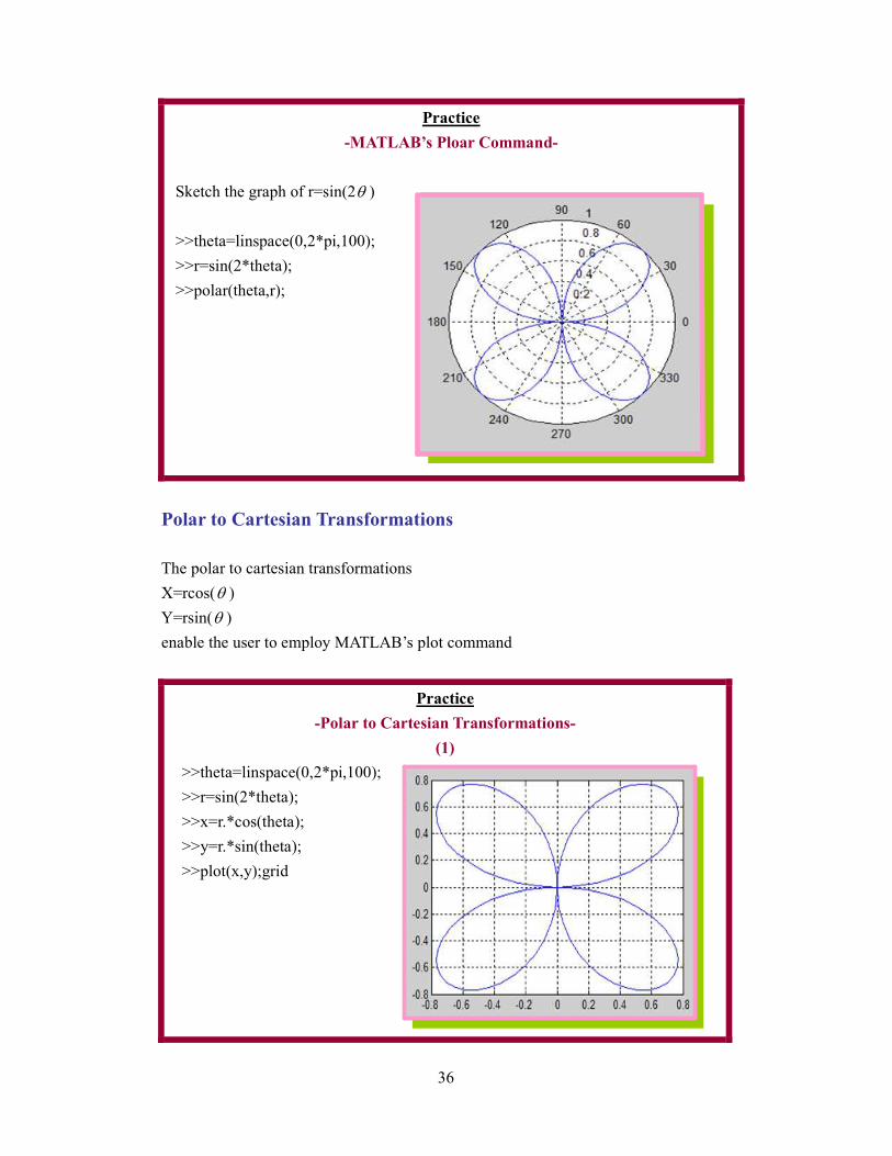
Practice
-MATLAB’s Ploar Command-
Sketch the graph of r=sin(2θ )
>>theta=linspace(0,2*pi,100);
>>r=sin(2*theta);
>>polar(theta,r);
Polar to Cartesian Transformations
The polar to cartesian transformations
X=rcos(θ )
Y=rsin(θ )
enable the user to employ MATLAB’s plot command
Practice
-Polar to Cartesian Transformations-
(1)
>>theta=linspace(0,2*pi,100);
>>r=sin(2*theta);
>>x=r.*cos(theta);
>>y=r.*sin(theta);
>>plot(x,y);grid

37
Practice
-Polar to Cartesian Transformations-
(2)
The plot command, which directly plots vectors of magnitude and angle, is polar.
The equation of cordioid in polar form, with parameter a is given by
( )( )1 cosr a θ= + , 0 2θ π≤ ≤
>>a=1;
>>theta=0:2*pi/200:2*pi;
>>r=1+cos(theta);
>>polar(theta,r)
Line, Marks and Colors
- Basic Functions
When plotting multiple curves, it is desirable to vary the colors, plot symbols and line
styles (dashed, dotted, etc.) associated with each line. This feature is accomplished
by adding another argument to the plot command.
��NOTE��
Line styles and marks allow you to discriminate different data sets on the same plot
when color is not available.
� Syntax
>>plot (x,y, ‘linestyle_mark_color’);
with no separators between the options. The options can be in any order.

38
Practice
-Lines, Marks & Colors-
>>plot(t,y,’:’); % plot y versus t using a dotted line
>>plot(t,y,’r:’); % plot y versus t using a dotted line in red
>>plot(t,y,’-.ro’); % plot y versus t using a dash-dot line (-.),
colored red (r) and (o) at the data points
>>% and place places circular maker
Symbol of Lines, Marks & Colors
The line styles and colors consist of character string whose first character specifies the
color (optional) and second the line style, enclosed in single quotes. The options for
line styles, marks, and color are depicted below.
Symbols of Line:
LINE SYMBOL
Dash --
Dashdot -.
Dotted :
Solid -(default)
Symbols of Color:
COLOR SYMBOL
Blue b
Black k
Cyan c
Green g
Magenta m
Red r
Write w
Yellow y
Symbols of Mark:
MARK SYMBOL
Circle O
Point .
Plus +
Star *
X-mark x
Square s
Diamond d
Pentagrom p
Hexagram h

39
Practice
- Symbols of Lines & Color-
(1)
>>t=0:0.01:2 % define a time vector
>>y=cos(2*pi*4*t) % define a vector y
>>plot(t,y,’*r’) % plot y versus t by (*) marks in red color
Practice
- Symbols of Lines & Color-
(2)
>>%Taylor series approximation of exp(x) near x=1
>>x=0:0.01:3;
>>p1=exp(x);
>>p2=exp(1)+exp(1)*(x-1);
>>p3=exp(1)+exp(1)*(x-1)+exp(1)*(x-1).^2/2;
>>p4=exp(1)+exp(1)*(x-1)+exp(1)*(x-1).^2/2+exp(1)*(x-1).^3/6;
>>plot(x,p1,'m-',x,p2,'g--',x,p3,'r-',x,p4,'k:','LineWidth',3)
>>legend('exp(x)','n=1','n=3','n=3')
>>title('Taylor series approximation of exp(x) near x=1', 'Fontsize',12)
>>xlabel('x','Fontsize',13)
>>ylabel('e^{x}','FontSize',13)
>>grid

40
Graphics Handles
When using the plotting command, MATLAB draws the graph using a number of
graphics objects, such as line, text, and surfaces. All graphics objects have a set of
properties that control the appearance and behavior of the object. For example a line
is an object with properties such as line style, color, and thickness. It is possible,
under MATLAB, to access and modify these properties.
A. The Main Functions
MATLAB assigns a unique identifier to every object in the figure window. This
number is called the handle of the object. The handle of the figure is an integer, and
all other handles are floating-point numbers. You can use this handle to access the
object’s properties. The commands xlabel, ylabel, title and text return handles to the
objects they create.
>>h1=plot(x,y,’mo’); % make a plot and return graphics object handle
>>h2=xlabel(‘time,[s]’); % label the horizontal axis and return handle
>>h3=ylabel % label the vertical axis and return handle
The variable h1, for example, holds information about the graph you generated and is
called the handle graphics. You may view the list of properties and their values with
command get(handle).
Practice
-“Graphics Handles: The Main Functions-
>>t=0:0.01:2; % define the time vector
>>y=sin(2*pi*3*t); % specify the corresponding y-vector
>>h1=plot(t,y); % generate a plot and return handle
>>h2=xlabel(‘time,[s]’; % label the time axis and return handle
>>h3=ylabel(‘Amplitude,[v]’); % label the voltage axis and return handle
>>h4=title(‘Sine wave’); % add title and return handle
>>get(h2) % list all properties of h2 and their values
(Continue on next page)

41
Color = [0 0 0]
EraseMode = normal
Editing =off
Extent = [0.87468-1.35849 0.234294 0.169811]
FontAngle = normal
FontName = Helvetica
Fontsize = [10]
FontUnits = points
FontWeight =normal
HorizontalAlignment = center
Position = [0.997436-1.22275 17.3205]
Rotation = [0]
String =time,[s]
Units=data
Interpreter = tex
VerticalAlignment = cap
BeingDeleted = off
ButtonDownFcn =
Children = []
Clipping = off
CreateFcn =
DeleteFcn =
BusyACtion = queue
HandleVisibility = off
HitTest = on
Interruptible = on
Parent = [100.001]
Selected = off
SelectionHighlight = on
Tag =
Type = text
UIContextMenu =[]
UserData=[]
Visible = on

42
B. Additional Functions
- “gcf”, “gca” & “gco”
There are several functions that are useful for accessing handles of current objects.
These are:
gcf(get current figure) % return the handle of current figure
gca(get current axis) % return the handle of current axes
gco(get current object) % return the handle of current object
★ Syntax
>>h2=get(gca,’xlabel’)
>>h3=get(gca,’ylabel’)
>>h4=get(gca,’title’)
% provide handle of xlabel
% provide handle of ylabel
% provide handle of title
The following commands provide the list of properties:
>>get(gcf)
>>get(gca)
>>get(gco)
% list all properties of the figure
% list all properties of the axes
% list all properties of an object
C. The “set” Command
The set function allows the setting of object’s property by specifying the object’s
handle and any number of property name/property value pairs.
� Syntax
>>set(handle,’property_name’, property_value)
For instance, to change the color and width of the line, proceed as follows:
>>set(handle, ‘color’, [0 0.8 0.8], ‘LineWidth’, 3)
To obtain a list of all settable properties for a particular object, call set with the object’s
handle.
>>set(handle)

43
Practice
- Graphics Handles: Additional Functions & The “set” Command-
>>t=0:0.01:2; % define time vector
>>x=3+2*cos(2*pi*3*t); % define the dependent vector x
>>h1=plot(t,x); % plot and get handle
>>set(hi,’LineWidth’,3); % set thickness to 3
>>h2=xlabel(‘time,[s]’); % label axis and get handle
>>set(h2,’FontSize’,13); % set the font size of x-label to 13
>>set(gca,’Xtick’,0:0.25:2); % set X-tick
>>h3=ylabel(‘Amplitude,[v]’); % label axis and get handle
>>set(gca,’Ytick’,0:0.5:5); % set Y-tick
>>set(h3,’FontSize’,13); % set font size of y-label to 13
>>h4=title(‘Sinusoidal waveform’); % add title and get handle
>>set(h4,’color’,[0.6 0.3 0.4],’FontSize’,13); %set color and font size of title
D. Additional Information
It is also possible to change the attributes of the line width and the marker colors with
commands like:
LineWidth
MarkerEdgeColor
MarkerFaceColor
MakerSize
Width (in points) of the line
Color of the marker or the edge color four filled markers
Color of the face of filled markers
Size of the maker in points
Once a waveform is plotted, one can change the style and feel by providing additional
information.

44
Practice
- Graphics Handles: Additional Information-
>> x=linspace(0,2*pi,60);
>> y=sin(2*x);
>> plot(x,y,'-mo','LineWidth',2,...
'MarkerEdgeColor','k',...
'MarkerFaceColor',[.48 1 .62],...
'MarkerSize',10)
This script produces a plot of sin(3x) using a solid magenta line of width 2 point
drawn with circular markers of size 10 point at the grid nodes which are colored
mint green internally and have a black edge.
Commands
A. “figure(n)” Command
When the plot command is executed, a graphics window appears automatically. It is
possible to open as many figure windows as memory permits. To create a new
window use the command figure(n). MATLAB numbers figure windows starting at 1.
>>figure(2); % pop up a new graphics window
B. “clf” & “close(n)” Commands
A Figure can be cleared using the clf command, and closed by entering close(n) when
n is the number of the window to close.

45
Overlaying Plots
It is often desirable to overlay two plots on the same set of axes. To overlay plots, you
tell MATLAB to hold the previous plot using hold on and subsequent graphs will be
on the same axes. The hold command will remain active until it is turned off, by
entering hold off.
Practice
-Overlaying Plots-
(1)
>>t=0:0.01:2; % define a time vector
>>y=cos(2*pi*4*t); % define vector y
>>plot(t,y); % plot y versus t
>>z=sin(2*pi*3*t); % define vector z
>>hold on % hold the previous plot
>>plot(t,z) % overlay plots
>>hold off % turn off the hold function
Similarly, several signals with equal number of data points may be displayed in the
same frame against the same axis as follows:
Practice
-Overlaying Plots-
(2)
>>t=0:0.01:2 % define a time vector
>>x1=sin(2*pi*3*t); % define vector x1
>>x2=cos(2*pi*2*t); % define vector x2
>>x3=abs(x2); % define vector x3
>>x=[x1;x2;x3]; % matrix of data
>>plot(t,x); % plot 3 signals against time
If, on the other hand, the curves are plotted against different vectors, we use,
>>plot(t2,x2,t2,x2,t3,x3)

46
This command plots x1 versus t1, x2 versus t2, and x3 versus t3. In this case, t1,t2,
and t3 may be of different sizes, provided that x1, x2, and x3 are of the same size as
their corresponding time vector t1, t2, and t3, respectively.
Practice
-Overlaying Plots-
(3)
>>plot(t1,x1,’r’,t2,x2,’g’) % plot x1 in red and x2 in green
Plotting Practices
Practice
- Plotting Practice-
(1)
Plot the discrete-time signal specified by x[n] =cos 213
nπ
>>n=0:1:24; % define a vector n
>>x=cos(2*pi*n/13); % define vector x
>>stem(n,x) % plot x versus n
Practice
-Plotting Practice-
(2)
We shall try now semilog plots.
>>t=linspace(0,2*pi,200);
>>x=exp(-2*t)
>>y=t;
>>semilog(x,y);grid
% generate 200 linearly spaced points in [0.2π]
% define the function x(t)
% define the function y(t)
% provide a semilog plot of y versus x
The command grid will place grid lines on the current graph.
47
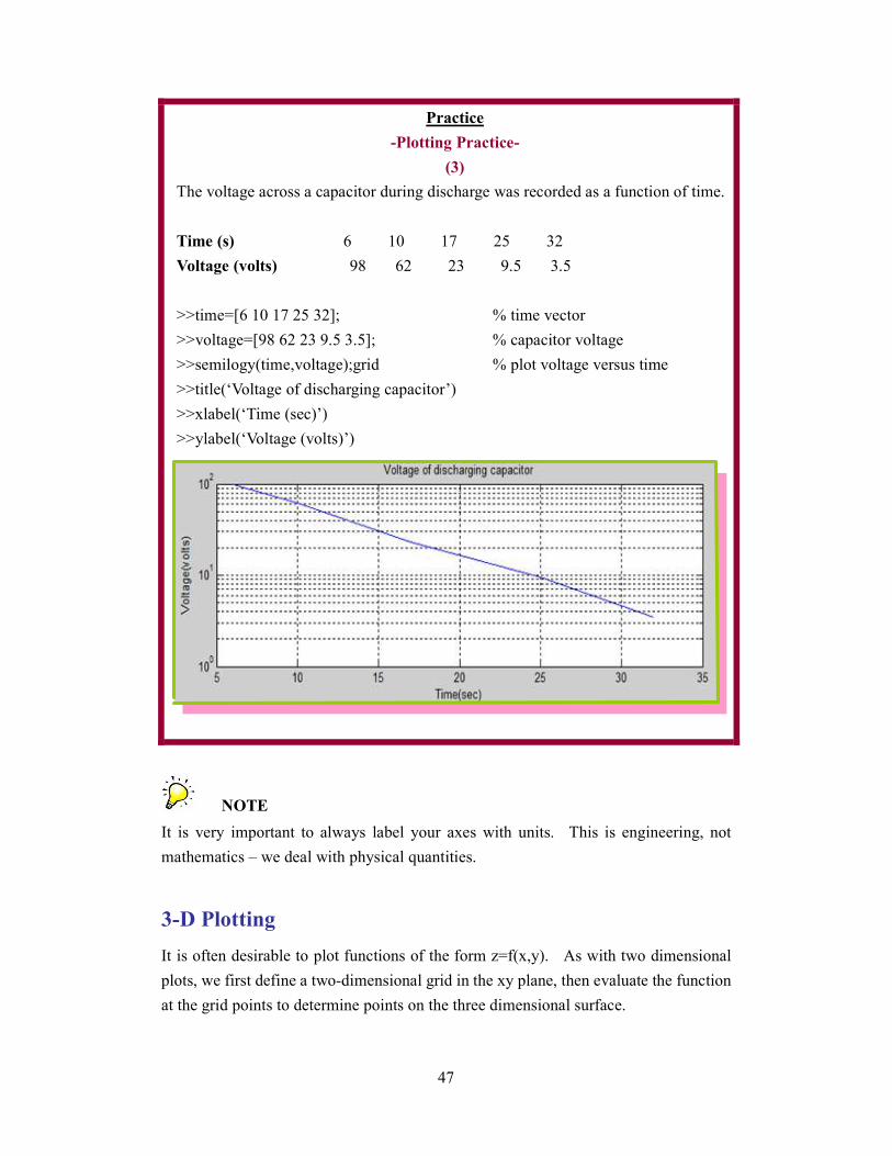
Practice
-Plotting Practice-
(3)
The voltage across a capacitor during discharge was recorded as a function of time.
Time (s) 6 10 17 25 32
Voltage (volts) 98 62 23 9.5 3.5
>>time=[6 10 17 25 32]; % time vector
>>voltage=[98 62 23 9.5 3.5]; % capacitor voltage
>>semilogy(time,voltage);grid % plot voltage versus time
>>title(‘Voltage of discharging capacitor’)
>>xlabel(‘Time (sec)’)
>>ylabel(‘Voltage (volts)’)
��NOTE��
It is very important to always label your axes with units. This is engineering, not
mathematics – we deal with physical quantities.
3-D Plotting
It is often desirable to plot functions of the form z=f(x,y). As with two dimensional
plots, we first define a two-dimensional grid in the xy plane, then evaluate the function
at the grid points to determine points on the three dimensional surface.

48
A two-dimensional grid in the xy plane is defined in MATLAB by two vectors, one
containing the x-coordinates at all points in the grid, and the other containing the
y-coordinates. When you want x and y to vary over some range, you need a matrix
(rather than a vector) for x and y to get a complete domain that covers all the different
combinations of those x and y values over some range. The meshgrid function
creates 2 matrices X and Y from the x and y vectors. The rows of the resulting matrix
X are formed by repeating the vector x and the columns of the matrix Y are formed by
repeating the vector y.
Practice
-3-D Plotting-
(1)
x=-2:2;
y=-3:3;
[X,Y]=meshgrid(x,y)
(X,Y)=(-2,0)

49
Practice
-3-D Plotting-
(2)
>>x=0:0.01:10;
>>y=x;
>>[X,Y]=meshgrid(x,y);
>>Z=3*sin(sqrt(X.^2+Y.^2));
>>mesh(X,Y,Z)
Practice
-3-D Plotting-
(3)
>>x=-2:0.1:2;
>>y=-3:0.1:3;
>>[X,Y]=meshgrid(x,y);
>>Z=exp(-(X.^2+Y.^2));
>>surf(X,Y,Z)

50
Changing the Viewing Direction
Viewing the surface from different angles: The viewing angle is specified by the view
command – view(az,el) where az is the azimuth in degrees, measured positive
counterclockwise, and el is the elevation in degrees above the xy plane. The default
view is (-37.5, 30).
3-D Plotting Table
The following Table summarizes the most popular 3D plotting functions.
3D Plotting Functions
Matlab Command Meaning
plot3 Simple x-y-z plot
contour Contour plot
contourf Filled contour plot
contour3 3D contour plot
mesh Wireframe surface
meshc Wireframe surface plus contours
meshz Wireframe surface plus curtain
surf Solid surface
surfc Solid surface plus contour
waterfall Unidirectional wireframe
bar3 3D Bar graph
bar3h 3D Horizontal bar graph
pie3 3D Pie chart
fill3 Polygon fill
comet3 3D Animated, comet-like plot
scatter3 3D Scatter plot
stem3 Stem plot

51
Contour Plots
Both 2D and 3D contour plots can be produced. contour(z) produces a 2D plot of the
matrix z, when the z values are treated as heights above the 2D plane. It is also
possible to override the default number of contour lines (20) by choosing the number
of lines required; for example, for integer N,
Practice
-Contour Plots-
>>z=peaks(24);
>>figure;
>>subplot(1,2,1); contour(z);
>>subplot(1,2,2; contour (z,10);
Bar Graph
A bar graph is a diagram that compares bars of the same width but of different heights
according to the data they represent. A bar graph may be horizontal or vertical. Bar
graphs are one of the many techniques used to present data in a visual form in order to
recognize patterns or trends.
Practice
-Bar Graph-
(1)
>> x=-3:0.2:3;
>>y1=sin(x); y2=sin(x)/2;
>>subplot(2,2,1);bar(x,y1);title('2-D Bar graph--vertical')
>>subplot(2,2,2);bar3(x,y1);title('3-D Bar graph')
>>subplot(2,2,3);barh(x,y1);title('2-D Bar graph--horizontal')
>>subplot(2,2,4);bar(x',[y1' y2'],'stacked');title('2-D Bar graph--stacked')

52
Practice
-Bar Graph-
(2)
>>x=[1 2 3 4];
>>b1=[3 5 7 9];
>>b2=[1.5 2.7 3.2 6.7];
>>b=[b1;b2]’;
>>bar(x,b,’grouped’); colormap(cool)
Pie Charts
A pie chart is a circle graph divided into pieces, each displaying the size of some
related piece of information. A pie chart is produced with the command pie(x); it is
also possible to “explode” one or more segments of the pie for emphasis.
Practice
-Pie Charts-
(1)
Enrollment data in the school of engineering at a local university is summarized in
the following table:
Engineering Discipline No. of Students Fraction of Total
Civil
Electrical
Industrial
Mechanical
Chemical
Total
480
908
240
620
140
2388
0.20
0.38
0.10
0.26
0.06
1.00
Draw a pie chart of the distribution of students in the school of engineering.
>>x=[480 908 240 620 140];
>>y={‘civil’,’Electrical’,’Industrial’,’Mechanical’,’Chemical’}
>>pie(x,y)

53
Practice
-Pie Charts-
(2)
>>x=[1.3 2.5 4.4 6.7];
>> subplot(2,2,1);pie(x);
>>subplot(2,2,2); pie(x,[0 0 0 1])
>>subplot(2,2,3);pie(x,{'GM','IBM', 'DELL','HP'});
>>subplot(2,2,4);pie3(x,[0 1 0 0])
Subplots
MATLAB graphics window accommodates a single plot by default, but it is possible to
create an array of subplots within the one figure. The subplot command allows a
given figure window to be broken into a rectangular array of plots, each addressed with
the standard plot commands.
>>subplot(r,c,w)
The arguments r and c are the number of rows and columns into which the graphics
window is divided, respectively. The w designates the position of the graph.
Windows are numbered from left to right and top to bottom within the figure. For
example, subplot(2,1,1) partition the graphics window into two rows in a single
column and fits the plot on the top cell. Figure 1 depicts two possible subplots
arrangement.

54
2 rows
2 rows
Customizing Plots
A. Basic Functions
-Commands: “title”, “xlabel”, “ylabel”, “grid” & “legend”
MATLAB provides means to improve the appearance and clarity of the plots. Once a
plot is on the screen, it may be given a title, axes labeled and text placed within the
graph. The title command is used to place a title above the plot, xlabel writes text
beneath the x-axis, and ylabel writes a text besides the y-axis of a plot. They each
take a string variable, which must be in single quote. The grid command toggles a
grid on and off in the current figure, the legend commend adds a legend to an existing
graph (movable with the mouse) that automatically uses the right symbols and colors
and sticks the description in the legend command after them, and the text command
allows a string of text to be placed at a particular x-y position on the graph.
� Syntax
>>xlabel(‘label’); % write label beneath the x-axis
>>ylabel(‘label’) % write label besides the y-axis
>>title(‘label’); % place a title above the plot
>>text(x,y,’label’); % write label at the location(x,y)
>>grid % draw a grid on the graph area
>>legend(‘first plot’, ‘second plot’); % place a legend within a graphics window
��Note��
It is very important to always label your axes with units. This is engineering, not
mathematics – we deal with physical quantities.

55
Practice
-Customizing Your Plots-
(1)
>>t=-2*pi:0.02:2*pi; % define a time vector
>>y=sin(t).*cos(t).^2; % define a dependent vector y
>>plot(t,y);grid; % plot y versus t
>>xlabel(‘time,[s]’) % annotate the t-axis
>>ylabel(amplitude,[v]; % annotate the y-axis
>>legend(‘trig function’) % add a legend to plot
B. Interactive Labeling & Coordinates of Points
-Commands: “gtext” & “griput”
The gtext command provides interactive labeling. After generating the plot, enter the
following command:
>>getext(‘label’)
This command places text on the graph by showing a crosshair on the graphics window.
After the crosshair is positioned where you want the text to appear, press the mouse
button. The griput command determines the coordinates of points on the graph.
>>[x,y]=ginput(n); %provide coordinates of n points on a graph
Position the mouse cursor on a point of a graph for which you want to know the
coordinates, and click the mouse button, then repeat the process for the remaining (n-1)
points. When done, hit the carriage return (enter key), and the n-coordinates will be
shown on the command window.
C. Redefine Your Axis
-Commands: “axis”, “axis(‘square’), “axis off” & “axis on”
MATLAB automatically selects the appropriate ranges and tick marks for the graph,
but it is often necessary to redefine it. The axis command manually sets the axis
limits. This command is implemented as follows:
>>axis([xmin xmax ymin ymax])

56
where xmin xmax ymin ymax are the desired maximum and minimum values for the
x and y axes, respectively.
The command axis(‘square’) ensures that the same scale is used on both axes. You
can remove the axes from your graph and put them back via axis off and axis on,
respectively.
The following Table shows a list of Matlab commands used to control the axes.
Some Matlab Commands for Controlling the Axes
Mathematical notation: Meaning:
axis([xmin xmax ymin ymax]) Set specified x- and y-axis limits
axis auto Return to default axis limits
axis equal Equalize data units on x-, y- and z-axes
axis off Remove axes
axis on Put axes back
axis square Make axis box square (cubic)
axis tight Set axis limits to range of data
xlim([xmin xmax]) Set specified x-axis limits
ylim([ymin ymax]) Set specified y-axis limits
Practice
-Customizing Your Plots-
(2)
Use the plot command to draw a circle.
>>t=0:pi/100:2*pi; % time base
>>plot(sin(t),cos(t)); % draw circle
>>axis(‘square’) % use same scale on both axes

57
Practice
-Customizing Your Plots-
(3)
>>t=0:0.01:1; % generate a time vector t
>>y=sin(2*pi*5*t); % define the dependent vector y
>>x=y+cos(2*pi*5*t); % define the dependent vector x
>>z=abs(y); % define the dependent vector z
>>w=1./(1+t.^2); % define the dependent vector w
>>subplot(2,2,1);plot(t,y);grid; % split screen, plot y versus t, and apply grid lines
>>ylabel(‘Voltage,[V]’); % label the vertical axis
>>subplot(2,2,2);plot(t,x);grid; % plot x versus t, and apply grid lines
>>ylabel(‘Current, [A]’); % label the vertical axis
>>subplot(2,2,3);plot(t,z);grid; % plot z versus t, and apply grid lines
>>ylabel(‘Power,[W]’); % label the vertical axis
>>subplot(2,2,4);plot(t,w);grid; % plot w versus t
>>ylabel(‘Voltage,[V]’); % label the vertical axis
Creek Letters, Subscripts, & Superscripts
A. Greek Letters
When you add labels and titles on your plot, you may want to use Greek letters,
subscripts and superscripts. To get Greek letters, simply type their names preceded
by a backslash as follows:
\alpha \beta \gamma \delta \epsilon \phi
\theta \kappa \lambda \mu \pi \rho
\sigma \tau \xi \zeta \omega

58
Practice
- Greek Letters-
>>label(‘H(\omaga)’)
You can also use capital Creek letters, like this, \Gamma
B. Subscripts
To put a subscript on a character use the underscore character on the keyboard: 1µ is
coded by typing \mu_1. If the subscript is more than one character long, such as 12µ ,
use this: \mu_{12}.
C. Superscripts
Superscript work the same way only use the ^ character: \theta^{10} to get 10θ .
- Script Files and Function Files
Introduction
MATLAB operates in two modes:
□ The interactive mode
□ The batch mode
Thus far we considered only the command-driven mode (interactive mode). Under
this mode MATLAB processes the statement and display the result immediately.
MATLAB is also able to execute (batch mode) programs that are saved in files. These
files must be in ASCII format and have an extension .m (for example prog1.m). This
is the reason why MATLAB files are called M-files. There are two types of M-files:
script files and function files.

59
Script Files
A script file is an ordinary text file that contains a sequence of MATLAB statements.
Variables in a script file are global. These files offer a more effective working
environment and allow files to be saved for future use. To execute a script file,
simply type the filename (without the extension) at the MATLAB command window.
To make a script file, I suggest you create a temporary sub-directory for all your work,
like c:\myfiles, start MATLAB and change its working directory to c:\my files, via the
cd command, as you would in DOS and UNIX. To use a floppy disk as the storage
location, which is an excellent idea since you can take your work with you when you
leave the computer lab, put a formatted floppy disk in the computer and type cd a:\ as
follows:
>>cd a:\ <enter> % change the current directory to a:
The following commands facilitate moving around directories:
>>! mkdir c:\mlab % create a sub-directory named mlab
>>!rmdir c:\mlab % remove the sub-directory mlab
>>cd c:\mlab % change the working directory to mlab
>>pwd % show current working directory
>>dir % list the contents of the current directory
>>what % list only the M-files in the current directory
>>ls % show a list of files in the working directory
>>delete filename.m % delete a specified file
>>type filename.m % print a specific file to the screen
>>which filename.m % find the current path
��NOTE��
In the CAEC (or ECE labs) cluster, all directories on the hard disk are write protected,
in order to avoid accumulation of files. The best practice is to use a floppy disk for
your M-files.

60
Example
-Script Files-
As an example, let us create a script file named, toto.m. The script file can created
and edited using any ASCII editor, such as notepad or the built-in MATLAB editor,
which color codes reserved words and other program elements. You bring up the
MATLAB text editor window by clicking the editor icon on the toolbar (or choose
New, then M-file under the File pull-down menu or launch it by typing edit from
within MATLAB environment). Then enter the script file in the editor window, as
follows:
After you have typed in the script file, you should save it in the newly created
sub-directory. To do this, select Save As under the File menu item from the editor’s
menu bar. When the save dialog box opens, type in the name toto.m and click on
save. Return to the MATLAB command window.
To run the script, simply type,
>>toto <enter>

61
If there are errors, MATLAB will beep and display error messages in the command
window. Return to the MATLAB editor to debug the original script, save the changes
and run it again. To open an existing M-file, choose Open under the File menu and
select the file for editing.
Function Files
MATLAB has many powerful built-in functions. MATLAB also allows for user to
write their own functions. Functions are identical to script files, except that variable
values may be passed into or out of the function file. The function file starts with the
keyword function and defines the function name and input and output variables. The
function file starts with the keyword function and defines the function name and input
and output variables. The format of the first statement for a function named toto is of
the form
Function [output1,output2,output3,…] = toto(input1,input2,input3,…)
There the input variables are enclosed within parentheses while output variables are
within square brackets if there is more than one output variable.
Example
- Function Files-
As an illustration, let us create the function magphase.m, which computes the
magnitude and phase of a complex number z supplied by the user.
Invoke the built-in MATLAB editor and enter the following lines of code:
function [m,p]=magphase(z) % specify a file as a function file
% z is a complex number supplied by the user (input variable)
% m and p are output variables representing the magnitude and phase of z
% magphase is the function name
m=abs(z);
p=angle(z)*180/pi;
% compute the magnitude of z
% compute the phase in degrees
( Continue on next page)
62
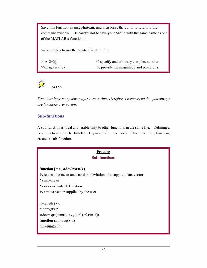
Save this function as magphase.m, and then leave the editor to return to the
command window. Be careful not to save your M-file with the same name as one
of the MATLAB’s functions.
We are ready to run the created function file.
>>z=2+3j; % specify and arbitrary complex number
>>magphase(z) % provide the magnitude and phase of z.
��NOTE��
Functions have many advantages over scripts, therefore, I recommend that you always
use functions over scripts.
Sub-functions
A sub-function is local and visible only to other functions in the same file. Defining a
new function with the function keyword, after the body of the preceding function,
creates a sub-function.
Practice
-Sub-functions-
function [mn, stdev]=stat(x)
% returns the mean and standard deviation of a supplied data vector
% mn=mean
% stdev=standard deviation
% x=data vector supplied by the user
n=length (x);
mn=avg(x,n)
stdev=sqrt(sum((x-avg(x,n)).^2)/(n-1))
function mn=avg(x,n)
mn=sum(x)/n;

63
- inline functions
You can create your own functions to use in MATLAB. If your function is simple
enough (i.e., ( ) 2 3 5f x x x= + + ), then MATLAB has a command inline used to
define the so-called inline functions in the command window. Let us say we want to
define the function ( )23xg x xe−= , we can proceed as follows:
>>g=inline(‘x.*exp(-3*x.^2)’,’x’);
You can evaluate this function in the usual way
>>g(1)
You can apply this function to a scalar or vector
>>g([0 1 2]) or
>>g([0:4])
Furthermore, the defined function can be plotted in a specified interval as follows:
>>fplot(g,[0 2]) % plot g(x) over 0 2x≤ ≤
Commands going to be introduced in this section include:
echo
pause
pause (n)
input
find
zoom on
zoom off
There are some special functions that can be very helpful when included in M-files.
The echo command display each command in your script on the MATLAB command
window, as the script is being executed. The pause command causes a routine to stop
executing. This last command gives you time to check your results. Striking any

64
key will cause the script file to resume operating. The command pause(n) will pause
execution for n seconds. The input command prompts the user for a numeric or
string input data from the keyboard during program execution. The disp command
displays scalar, vector, matrix or a string on the command window without variable
name. The function find returns a list of indices of the elements of a vector or matrix
that satisfy some condition. The zoom command provides a means to zoom on any
part of a 2-D graph and see it enlarged in the plot window. The statement zoom on
turns on the zoom mode. Then, to zoom in about a particular point on the graph,
move the cursor to the point and click with the mouse. This action expands the plot
by a factor of 2 centered on that point. To zoom out by a factor of 2, click the right
mouse button. The command zoom off turns off the zoom mode.
Practice
- Additional Commands-
t=-1:0.06:1; % time base
f=input(‘Enter the frequency of the sine wave:’); % input from keyboard
disp([‘frequency:’,intstr(f)]) % print the value of frequency
x=sin(2*pi*f*t).*exp(-x.^2); % wave
plot(t,x,’:’,’LineWidth’,2); % plot wave
disp(‘Press any key to continue’)
pause; % pause execution
hold on % hold previous plot
k=find(x>0.3) % find indices for which x>0.3
plot(t(k),x(k),’ro’,’LineWidth’,2); % plot x(k) vs t(k)
disp(‘Press any key to continue’)
pause % pause execution
m=find(t>0.4 & x<0) % find m’s such that t>0.4 &
plot(t(m),x(m),’m-‘,’LineWidth’,2) % plot x(m) vs t(m)
xlabel(‘t’) % label horizontal axis
ylabel(‘x(t)’) % label the vertical axis
title(‘Illustration of the find function’) % add title
hold off
(The plot is shown on the next page)

65
��NOTE��
A string input can be typed from the keyboard, as follows:
>>str=input (‘what is the capital of Belgium?’,’s’);
The argument s specifies that the input form the keyboard is a string.
Introduction
Output data can be written from the computer onto a standard output device using the
function fprintf. The fprintf function has a unique format for printing constants and
variables. The fprintf function is also vectorized. This enables printing of vectors
and matrices with compact expression.
The “fprintf” Command
A. Display the Character String
>>fprintf(character string, arg2, arg2,…,argn)
The character string refers to a string that contains formatting information, and
arg1,arg2,…argn are arguments that represent the individual output data items.
Note that fprintf function can have one or more arguments enclosed within

66
parentheses. A comma separates these arguments. The first argument to the fprintf
routine is always the character string to be displayed.
B. Display the Value of Variables
However, along with the display of the character string, we may frequently wish to
have the value of certain program variables displayed as well.
fprintf(‘Programming in MATLAB is fun.\n’)
What does the function fprintf do with the argument? Obviously, it looks at whatever
lies between the single quotation marks and prints that on a terminal’s screen. The
characters \n included in the quotes does not get printed; it advances the screen
position by one line.
num=1;
fprintf(‘My favorite number is %d because it is first.\n’, num);
The fprintf function takes the value of the variable on the right of the comma and
plugs it into the string on the left. Where does it plug it in? Where it finds a format
specifier such as %d. Format specifier tells fprintf where to put a value and what
format to use in printing the value. The %d tells fprintf to print the value 1 as a
decimal integer. Other specifiers could be used for the number 1. For instance %f
would cause the 1 to be printed as a floating-point number. In addition to specifying
the type of conversion (e.g., %d, %f, %e) one can specify the width and precision of
the result of the conversion.
� Syntax
%wd
%w.pe
%w.pf
w: the number of characters in the width of the final result
p: represents the number of digits to the right of the decimal point

67
Illustration
-Formatted Output-
%12.3f use floating-point format to convert a numerical value to a string 12
characters wide with 3 digits after the decimal point.
The fprintf function can also be used to write formatted output into a file:
>>fprintf(‘file’, ‘area=%4.2f\n’, area)
The following table provides a list of the conversion character.
CHARACTERS DESCRIPTION
%s Format as a string
%d Format with no fractional (integer format)
%f Format as a floating-point value
%e Format as a floating-point value in scientific notation
%g Format in the most compact form of either %f or %e
\n Insert newline in output string
\t Insert tab in output string
Practices of Formatted Output
Practice
-Formatted Output
(1)
>> A=[1 2 3; 4 5 6; 7 8 9];
>>fprintf(‘%8.2f %8.2f %8.2f\n’,A)
1.00 4.00 7.00
2.00 5.00 8.00
3.00 6.00 9.00

68
Practice
-Formatted Output
(2)
Write a MATLAB script that use a loop and the fprintf function to produce the
following table:
alpha sin(alpha) cos(alpha)
0 0.0000 0.0000 1.0000
π /4 0.7854 0.7071 0.7071
π /3 1.0472 0.8660 0.5000
π /2 1.5708 1.0000 0.0000
2π /3 2.0944 0.8660 -0.5000
π 3.1416 0.0000 -1.0000
4π /3 4.1888 -0.8660 -0.5000
5π /3 5.2360 -0.8660 0.5000
2π 6.2832 -0.0000 1.0000
>>alpha=pi*[0 1/4 1/3 1/2 2/3 1 4/3 5/3 2];
>>fprintf(‘alpha sin(alpha) cos(alpha) \n’)
>>for k=1:9
fprintf(‘%6.4f %9.4f %9.4f\n’ ,alpha(k), sin(alpha(k)), cos(alpha(k)))
end
Practice
-Formatted Output-
(3)
One can build labels and titles that contain numbers you have generated, simply use
MATLAB’s sprintf function, which works just like fprintf except that it writes into
a string variable instead of to the screen. You can then use this string variable as the
argument of the command xlabel, ylabel, and title.
(Continue on the next page)

69
>>theta=0:0.01:2;
>>x=cos(3*theta);
>>subplot(2,1,1);plot(theta,x)
>>s=sprintf(‘x(\\theta)=cos(%i\\theta)’,3);
>>title(s)
>>xlabel(‘\\theta’)
MATLAB has control statements similar to those in most high-level computer
languages. We shall begin with relational and logical operations. In this section you
should think of 1 as true and 0 as false.
Rational operators
Rational operators are used to assess if a statement is true or false. False is always
represented by 0, and MATLAB will consider any non-zero value to be true.
< less than
<= less than or equal
> greater than
>= greater than or equal
= = equal
~ = not equal

70
��NOTE��
“=” is used in an assignment statement while “= =” is used in a relation.
We illustrate the use of these operators in the following example;
Practice
- Rational Operators-
>> A=[ 1 2 3];
>> B=[5 4 3];
>>A<B
answer: 1 1 0
>>A~=B
answer: 1 1 0
>>A>=B
answer: 0 0 1
Logical Operators
You can join relational operators using the following logical operators
Operator Function Description
& and Returns 1 for every element location that is
true (nonzero) in both arrays, and 0 for all
other elements
| or Returns 1 for every element location that is
true (nonzero) in either one or the other, or
both, arrays and 0 for all other elements.
~ not Complements each element of input array, A.
xor logical exclusive or Returns 1 for every element location that is
true (nonzero) in only one array, and 1 for all
other elements.

71
Practice
-Logical Operators-
>>A=[1 0 1 1];
>>B=[0 1 0 0];
>> A & B
answer: 0 0 0 0
>>A | B
answer: 1 1 1 1
>>~A
answer: 0 1 0 0
>>xor(A,B)
answer: 1 1 1 1
Logical Functions
- Commands: “find”, “any”& “all”
A. The “find” Command
The find command is a powerful command that can be used to locate elements in a
vector that satisfy a certain criterion.
Practice
- The “find” Command-
(1)
>>x=[-3 0 7 5 -8 -9 0 4 5];
The find command will be used to locate two indices of all elements of x that satisfy
the relation x<0.
(Continue on next page)

72
>>index=find(x<0)
index = 1 5 6
>>x(index)
ans = -3 -8 -9
>>index2=find(x==0)
index2 = 2 7
>>x=(index2)
ans = 0 0
>>index3=find(abs(x)<4)
index3 = 1 2 7
>>x(index3)
ans = -3 0 0
Practice
- The “find” Command-
(2)
>>x=[-3 2 4 6];
>>disp(find(v>3))
4 6
>>disp(find(v>0))
2 4 6

73
B. The “any” & “all” Commands
MATLAB offers several handy logical functions for analyzing the results of relational
comparisons. These include any and all. The function any is used to determine if a
matrix or vector has at least one nonzero entry and the function all checks if all the
entries are nonzero. The output of these two functions is Boolean (‘1’ is true, and ‘0’
is false).
Practice
- The “any” & “all” Commands-
>>A=[0 0 0 0];
>>any(A)
ans =
0
>>B=[1 1 1 1 1 1];
>>all(B)
ans = 1
Loop Constructs
Programs for numerical simulation often involve repeating a set commands many
times. All of the loop structures in MATLAB are started with a keyword such as “for”,
or “while” and they all end with the word “end”.
A. “for loop”
It is often the case in programming that one wants to do something a fixed number of
times. The for loop can be used to execute a command or sequence of commands for
a specified number of iterations. The form of a for loop that is most commonly used
is:
>>for index= start : step : end
Command statements
end

74
The index is increased from start to end in steps specified by step. The following
example creates an array containing the squares of the numbers one through twelve.
Practice
-Loop Constructs: “for loop”-
(1)
>>for k=1:12
>>x(k)=k^2;
end
Practice
-Loop Constructs: “for loop”-
Nested Loops
(2)
>> for k=1:10
for m=1:4
x=0.005*k;
y=30*m;
z(k,m)=10*exp(-y*x)*cos(120*pi*x);
end
end
Practice
-Loop Constructs- “for loop”
(3)
Find the sum of the following series
s=1+3+5+7+…+99
>>s=0.0; % initialize the sum
>>for k=1:2:99 % running index
s=s+k; % update sum
end % end for
>>s <enter> % print value of sum

75
B. “while loop”
The second loop structure available in MATLAB is the while loop. While statements
allow us to repetitively execute a piece of code while a certain condition remains true.
The general form of a while loop is:
>>while condition
Command statements
end
>>
Practice
-Loop Constructs- “while loop”-
(1)
The following while loop counts the number of rolls needed by a die until a 6 comes
up.
>>rolls=1;
>>faceup=ceil(6*rand);
>>while faceup~=6
rolls=rolls+1;
faceup=ceil(6*rand);
end
>>disp([‘You rolled 6! It took’, int2str(rolls),’rolls’])
Practice
- Loop Constructs: “while loop”-
(2)
Enter and run the following MATLAB script file:
n=1;
while n<200
x=n*0.05;
y(n)=4.25*cos(x);
z(n)=-7.2*sin(x)
n=n+1;
end

76
Practice
-Loop Constructs: “while loop”
(3)
Calculate the squares of the integers from 1 to 20.
>>square=[];
>>k=1;
>>while k<=20
square[k]=k^2;
k=k+1;
end
>>
��NOTE��
As a rule it is best to avoid such loops (for & while), for they are not executed
efficiently in MATLAB.
Control of Flow
A. If statement
Like most programming languages, MATLAB uses the keyword if to implement the
basic decision making statement. The if statement itself will execute a single
statement of a compound statement when the controlling condition is true. It does
nothing when it is false.
★ Syntax
If condition
Command statements
end

77
Practice
-Control of Flow: If statement-
>>count=0; sum=0;
>>a=0;
>>if a<10
count=count+1;
sum=sum+a;
a=a+1;
end
B. The else clause
The else clause allows execution of one set of statements if a controlling condition is
true and a different set if the controlling condition is false.
� Syntax
>>if condition
command statements
else
command statements
end
C. Multiple choice elseif clause
When we nest several levels of if-else, it may be difficult to determine which
controlling condition must be true (false) to execute each set of statements. In this
case, the elseif clause is often used to make the program logic clearer.
� Syntax
>>if condition1
command statements
elseif condition2
command statements
elseif condition3
command statements
end

78
Practice
-Control of Flow: Multiple choice elseif clause-
Enter and run the following script file:
n=input(Enter a positive number: ‘);
if rem(n,3)==0
disp(“The number is divisible by 3’)
elseif (rem(n,5)==0
disp(“The number is divisible by 5’)
else
disp(‘The number is neither divisible by 3 nor by 5’)
end
D. The switch-case construct
The switch statement is similar to the elseif construct but has more flexibility and a
clearer format. It compares the input expression to each case value. Once the match
is found it executes the associated commands.
Practice
-Control of Flow: The Switch-case Construct-
(1)
% Four-function calculator
num1=input(‘Enter a number: ‘);
num2=input(‘Enter a number: ‘);
op=input(‘Enter the operation: ‘)
switch op
case ‘+’
x=num1+num2
case’-‘
x=num1-num2
case’*’
x=num1*num2
otherwise
x=num1/num2
end
(Continue on the next page)

79
Here is a sample interaction with the script file:
Enter the first number: 34
Enter the second number: 24
Enter the operation: ‘+’
x=58
Practice
- Control of Flow: The Switch-case Construct -
(2)
Generate a random integer x from the set {1,2,…,10}. If x=1 or x=2, then the
message probability = 20% is displayed on the screen. If x=3 or 4 or 5, then the
message probability = 30% is displayed, otherwise the message probability = 50% is
generated.
x=ceil(10*rand);
swich x
case {1,2}
disp(‘Prob=20%’)
case{3,4,5}
disp(‘Prob=30%)
otherwise
disp(‘Prob=50%)
end
- Fitting Polynomial Models to Data
It is common in engineering and science to obtain a set of data points from an
experiment or measurement and wish to fit a curve to the set of data points in order to
determine a mathematical model that describes the data and use this model to
interpolate the data.

80
MATLAB has two functions, polyfit and polyval, which can quickly and easily fit a
set of data in a least-squares sense. A least-squares fit is a unique curve with the
property that the sum of the squares of the difference between the fitted curve and the
given data points is a minimum.
Polyfit & Polyval
A. Polyfit
Polyfit generates a vector of coefficients, p, corresponding to the n-th order
polynomial that fits the data (x,y), in a least-squares sense. p is a row vector of length
(n+1) containing the polynomial coefficients.
( ) ( ) ( ) ( )11 2 ....n np x p x p x p n−= + + +
>>pcoeff=polyfit(x,y,n)
The output of this function is a vector pcoeff which includes the coefficients p(1),
p(2), …, p(n).
B. Polyval
The polyval function uses the coefficients generated from polyfit to evaluate the
polynomial specified by pcoeff for a given set of x values
>>polyval(pcoeff, x) .
Quality of Fit
The plot of the curve that represents the fitted polynomial overlaid on the data is a
convenient way of evaluating the quality of the fit. Using the coefficients determined
by polyfit, one can create such a plot as follows:
>>coef=polyfit(x,y,n);
>>x_fit=linspace(min(x),max(x),N);
>>y_fit=polyval(pcoeff,x_fit);
>>plot(x,y,’o’,x_fit,y_fit)
where N=number of points used to plot the fitted polynomial
n=order of the polynomial to be fitted

81
Practice
“Curve Fitting- The “ployfit” Command-
(1)
Find the third-order least squares regression polynomial for these data and use the
resulting model to predict the value of y for x=8.
x 1 2 3 4 5 6 7
y 2 8 26 50 140 224 350
>>x=[1 2 3 4 5 6 7];
>>y=[2 8 26 50 140 224 350];
>>p=polyfit(x,y,3) % third-order polynomial that fits the data
p =
0.5000 6.6429 -23.8571 20.8571
3 20.5 6.6429 23.8571 20.8571p x x x∴ = + − +
>>val=polyval(p,8) % predict the value of y using the given model
val =
511.1429

82
Practice
“Curve Fitting- The “polyfit” Command-
(2)
In this example we will generate the data from 2 340 7y x x= − + − with added
random error. The random error has a gaussian distribution with zero mean and a
standard deviation of unity. We will fit a cubic polynomial to the data, then plot the
two functions on the same frame to see if the fit is any good.
x=linspace(0,8,41);
y=-40+7*x.^2-x.^3;
y=y+6*randn(size(x));
xp=0:0.02:8;
n=3;
p=polyfit(x,y,n);
yp=polyval(p,xp);
subplot(2,1,1);plot(x,y,’o’,xp,yp,’LineWidth’,2); grid
title(‘cubic polynomial fit’)
ylabel(‘y’)
xlabel(‘x’)
axis([0 8 -80 60])

83
- The “interpl” Command
MATLAB has a built-in interpolation routine interp1. Suppose you are given a set of
data points {x,y} and you have a different set of x-values{ }ix for which you want to
obtain the corresponding{ }iy values by interpolating in the {x,y} data set. You can
accomplish this task by using one of these three flavors of the interp1. By default,
MATLAB uses linear interpolation between data points.
>>yi=interp1(x,y,xi,’linear’);
>>yi=interp1(x,y,xi,’cubic’);
>>yi=interp1(x,y,xi,’spline’);
% linear interpolation
% quadratic interpolation
% spline interpolation
Practice
-Interpolation: The “interpl” Command
%data set
>>inc=pi/5;
>>x=0:inc:2*pi;
>>y=sin(x);
>>xi=0:inc/20:2*pi;
>>%linear interpolation
>>yi=interp1(x,y,xi,yi,’linear’);
>>subplot(2,1,1);plot(x,y,’b-‘xi,yi,’r-‘);grid
>>%cubic interpolation
>>yi=interp1(x,y,xi,’cubic’);
>>subplot(2,1,2);plot(x,y,’b-‘xi,yi,’r-‘);grid

84
Introduction
Data file commands are used to save and load files in either standard ASCII text or the
more compact MATLAB binary format which uses the *.mat extension. The
binary .mat format is useful for files which will be used with MATLAB, while the
ASCII format is useful when working with other programs (such as a word processor),
or sharing data with others who may not have access to MATLAB.
Practice
-Saving & Loading of Data-
>>x=0:5;
>>y=rand(size(x));
>>[x’ y’]
ans =
0 0.9501
1.0000 0.2311
2.0000 0.6068
3.0000 0.4860
4.0000 0.8913
5.0000 0.7621
A. The “save” Command
The save command will save all of the user-generated variables. To save x, and y data
in the file my_data.mat, proceed as follows:
>>save my_data x y; % create the file my_data.mat
The file my_data.mat will appear in the current directory and contains x, and y.
The use of ASCII format, -ascii or /ascii is appended after the variable names:
>>save my_data x y-ascii; % create the text file my_data.dat

85
To verify that these files are valid we first clear the MATLAB workspace and load the
file back into the workspace.
B. The “Load” Command
The load command is used to restore the variables at a subsequent MATLAB session:
>>load my_data % load the .mat file
>>load my_data.dat % load the ASCII file


![Angel's Friends Love 1ª Temporada [Fanfic]](https://img.pdfslide.net/doc/110x75/55721219497959fc0b90079f/angels-friends-love-1a-temporada-fanfic.jpg)

![Angel's Friends Love 2ª Temporada [Fanfic]](https://img.pdfslide.net/doc/110x75/5572121e497959fc0b901168/angels-friends-love-2a-temporada-fanfic.jpg)


![Angel's Friends Love 3ª Temporada [Fanfic]](https://img.pdfslide.net/doc/110x75/55cf9cb9550346d033aad293/angels-friends-love-3a-temporada-fanfic.jpg)
