Embed Size (px)
Citation preview

University of Texas at El Paso University of Texas at El Paso
ScholarWorks@UTEP ScholarWorks@UTEP
Open Access Theses & Dissertations
2020-01-01
Effect Of Flow Velocity And Geometry On The Signal From A Effect Of Flow Velocity And Geometry On The Signal From A
Piezoelectric Flow Rate Sensor Piezoelectric Flow Rate Sensor
Jad Gerges Aboud University of Texas at El Paso
Follow this and additional works at: https://scholarworks.utep.edu/open_etd
Part of the Materials Science and Engineering Commons, Mechanical Engineering Commons, and the
Mechanics of Materials Commons
Recommended Citation Recommended Citation Aboud, Jad Gerges, "Effect Of Flow Velocity And Geometry On The Signal From A Piezoelectric Flow Rate Sensor" (2020). Open Access Theses & Dissertations. 3133. https://scholarworks.utep.edu/open_etd/3133
This is brought to you for free and open access by ScholarWorks@UTEP. It has been accepted for inclusion in Open Access Theses & Dissertations by an authorized administrator of ScholarWorks@UTEP. For more information, please contact [email protected].
EFFECT OF FLOW VELOCITY AND GEOMETRY ON THE SIGNAL FROM A
PIEZOELECTRIC FLOW RATE SENSOR
JAD GERGES ABOUD
Doctoral Program in Mechanical Engineering
APPROVED:
Norman D. Love, Ph.D., Chair
Yirong Lin, Ph.D.
Calvin M. Stewart, Ph.D.
Tzu-Liang (Bill) Tseng, Ph.D.
David Tucker, Ph.D.
Stephen L. Crites, Jr., Ph.D.
Dean of the Graduate School

Copyright ©
by
Jad Gerges Aboud
2020

EFFECT OF FLOW VELOCITY AND GEOMETRY ON THE SIGNAL FROM A
PIEZOELECTRIC FLOW RATE SENOR
by
JAD GERGES ABOUD, MSME
DISSERTATION
Presented to the Faculty of the Graduate School of
The University of Texas at El Paso
in Partial Fulfillment
of the Requirements
for the Degree of
DOCTOR OF PHILOSOPHY
Department of Mechanical Engineering
THE UNIVERSITY OF TEXAS AT EL PASO
December 2020

iv
Acknowledgments
I would first like to thank the people around me who have made this dissertation possible.
Two of the most influential people who have made this dissertation possible and supported me
continuously over the past five years are Reem Issa and Maher Aldeghlawi. They helped me in
countless ways, whether late dinner, running experiments, proofreading papers, principles
discussion, or just simply listening. They always encouraged me, and for these things, I am
thankful. I would also like to thank my mother. She has listened to me, always provided wise
counsel by sharing her experiences, and helped me in many more ways than I can describe. I would
also like to thank my father for being a model of hard work and dedication. Without both of you,
I would not achieve anything.
Next, I would like to extend my thanks to my committee chair Dr. Norman Love for his
guidance and for allowing me the opportunity to succeed. Over the last six years, he has sharpened
my technical abilities, taught me valuable lessons, encouraged me to carry out the program and
apply it to all aspects of life. From these lessons, I believe I have grown a great deal, albeit painfully
at times. I also thank Dr. Love for financially supporting me over the past four and a half years,
allowing me to focus solely on completing the degree.
I thank my committee chair, professor Dr. Love who has shown me what it is to be
dedicated and passionate about teaching. His understanding of engineering principles and
mathematics has helped me throughout the program and will stay with me after leaving. I also
thank Dr. David Tucker (Dave) from the National Energy Technology Laboratory (NETL) for his
guidance and advice throughout my project. I believe both my advisors have shown me how to
communicate through writing and speaking effectively.

v
Next, I would like to thank my other committee members Dr. Yirong Lin, Dr. Calvin
Stewart, and Dr.Tzu-Liang (Bill) Tseng, for their participation, time, and comments on this
dissertation.
Dear colleagues and friends in NETL at Morgantown, WV (Hybrid performance (HYPER),
and Chemical Looping Combustion); I am very grateful for their support and help through
technical discussions with me; these include Dr. Larry Shadle, Dr. Nana Zhou, Dr. Farida Harun,
and Mr. Selorme Agbelze. I also acknowledge the Center for Space Exploration Technology
Research (cSETR), faculties, and students for their friendships and help through logistic and
technical support. Also, I express gratitude to Dr. Ahsan Choudhuri, the director of cSETR, from
the University of Texas at El Paso
This material is based upon work supported by the Department of Energy/ National Nuclear
Security Administration under Awards Number(s) DE-NA0003330 and DE-FE-0029113.

vi
Table of Contents
Acknowledgments.......................................................................................................................... iv
Table of Contents ........................................................................................................................... vi
List of Tables ...................................................................................................................................x
List of Figures .............................................................................................................................. xiii
Chapter 1: Introduction and Background .........................................................................................1
1.1 Introduction ..........................................................................................................................1
1.2 Piezoelectricity .....................................................................................................................4
1.2.1 Manufacturing of Piezoelectric Ceramics ...................................................................7
1.2.2 Piezoelectric Materials as Energy Harvesters .............................................................9
1.2.3 Using Piezoelectric Materials as Flow Rate Sensors ................................................12
1.3 Piezoelectric Constitutive Equations .................................................................................15
1.4 Piezoelectric Coefficients ..................................................................................................18
1.4.1 Mechanical Piezoelectric Constant ...........................................................................18
1.4.2 Electrical Piezoelectric Constant ..............................................................................19
1.4.3 Elastic Compliance Constant ....................................................................................20
1.4.4 Dielectric Coefficient ................................................................................................20
1.4.5 Piezoelectric Coupling Coefficient ...........................................................................21
1.5 Piezoelectric Sensor ...........................................................................................................23
1.6 Dynamic Input Forces or Displacements ...........................................................................26
1.7 Electrical Outputs...............................................................................................................27
1.8 Signal to Noise Ratio .........................................................................................................28
1.9 Surge and Stall ...................................................................................................................29
1.10 Practical Relevance ..........................................................................................................33
1.11 Objective ..........................................................................................................................34
Chapter 2: Methodology ................................................................................................................36
2.1 Theory ................................................................................................................................36
2.1.1 Phase I: Piezoelectric as a Flow Rate Sensor and velocity profile. ..........................36
2.1.2 Phase II: Geometrical effect and Empirical Equation ...............................................40
2.2 Experimental Setup ............................................................................................................43

vii
2.2.1 Rectangular Test Section (RTS) Setup .....................................................................43
2.2.2 Circular Test Section (CTS) Setup ...........................................................................45
2.2.3 Geometrical test section (GTS) setup .......................................................................46
2.3 Piezoelectric Sensors .........................................................................................................48
2.3.1 Piezo-P ......................................................................................................................48
2.3.2 Piezo-A .....................................................................................................................49
2.3.3 Piezo-B ......................................................................................................................50
2.3.4 Piezo-C ......................................................................................................................51
2.3.5 Piezo-D .....................................................................................................................52
2.3.6 Piezo-E ......................................................................................................................53
2.3.7 Piezo-F ......................................................................................................................54
2.3.8 Piezo-G .....................................................................................................................55
2.3.9 Piezo-H .....................................................................................................................56
2.3.10 Piezoelectric Properties ...........................................................................................57
2.4 List of instrumentation .......................................................................................................58
2.4.1 DC Axial Compact fan .............................................................................................58
2.4.2 Power Supply ............................................................................................................59
2.4.3 Function Generator ...................................................................................................60
2.4.4 Hotwire Anemometer................................................................................................61
2.4.5 Oscilloscope ..............................................................................................................62
2.4.6 NI-9215 with BNC DAQ ..........................................................................................64
2.4.7 Department of Energy (DOE) / National Energy Technology Laboratory (NETL)
..................................................................................................................................65
2.5 Test Matrix .........................................................................................................................71
2.5.1 Phase-I: Piezoelectric as a Flow Rate Sensor ...........................................................71
2.5.2 Phase-II: Geometrical effect and Empirical Equation ..............................................73
Chapter 3: Results and discussion..................................................................................................75
3.1 Results and discussion for phase-I .....................................................................................75
3.1.1 Velocity Profile Results ............................................................................................75
3.1.2 Drag Force Results ....................................................................................................79
3.1.3 Voltage Output Results .............................................................................................80
3.1.4 Signal to Noise Ratio results .....................................................................................83

viii
3.2 Results and discussion for phase-II....................................................................................84
3.2.1 Velocity results .........................................................................................................85
3.2.2 Drag Force Vs. Velocity ...........................................................................................87
3.2.3 Voltage Output Vs. Drag Force ................................................................................95
3.2.4 Voltage Output Vs. Flow Rate ................................................................................105
3.2.5 Frequency response .................................................................................................124
3.2.6 Signal to noise ratio ................................................................................................125
3.2.7 Thickness Variation Results ...................................................................................126
3.2.8 Area to Thickness Variation Results.......................................................................128
3.2.9 Width variation results ............................................................................................130
3.2.10 Aspect Ratio Variation ..........................................................................................131
3.2.11 Piezo Empirical Equation .....................................................................................133
Chapter 4: Summary and Conclusions .........................................................................................140
4.1 Summary of the Results ...................................................................................................140
4.2 Conclusion .......................................................................................................................142
4.3 Future Work .....................................................................................................................142
References ....................................................................................................................................143
Appendix ......................................................................................................................................151
Appendix A ............................................................................................................................151
Appendix B ............................................................................................................................156
Appendix C ............................................................................................................................157
Appendix D ............................................................................................................................167
SigmaPlot Curve Fitting ..................................................................................................167
Assumption Checking ......................................................................................................167
Normality Testing. ...........................................................................................................167
Constant Variance Testing. ..............................................................................................167
P Values for Normality and Constant Variance. ..............................................................168
Fit Results ........................................................................................................................169
Residuals ..........................................................................................................................170
More Statistics .................................................................................................................172
Other Diagnostics.............................................................................................................173

ix
4.3.1 Rsqr ...........................................................................................................................176
4.3.2 Sigmoid Function ....................................................................................................176
Appendix E ............................................................................................................................177
SigmaPlot Reports for Curve Fitting ...............................................................................177
Piezo-A Report.................................................................................................................177
Piezo-B Report .................................................................................................................179
Piezo-C Report .................................................................................................................181
Piezo-D Report.................................................................................................................183
Piezo-E Report .................................................................................................................185
Piezo-F Report .................................................................................................................187
Piezo-G Report.................................................................................................................189
Piezo-H Report.................................................................................................................191
Empirical equation Report ...............................................................................................193
Appendix F.............................................................................................................................198
Phase II test Summary .....................................................................................................198
Vita 202

x
List of Tables
Table 1-1 Piezoelectric beam output equations [7] ....................................................................... 25
Table 2-1 Piezo-P dimensions ...................................................................................................... 48
Table 2-2 Piezo-A dimensions ...................................................................................................... 49
Table 2-3 Piezo-B dimensions ...................................................................................................... 50
Table 2-4 Piezo-C dimensions ...................................................................................................... 51
Table 2-5 Piezo-D dimensions ...................................................................................................... 52
Table 2-6 Piezo-E dimensions ...................................................................................................... 53
Table 2-7 Piezo-F dimensions ...................................................................................................... 54
Table 2-8 Piezo-G dimensions ...................................................................................................... 55
Table 2-9 Piezo-H dimensions ...................................................................................................... 56
Table 2-10 Piezoelectric Properties .............................................................................................. 57
Table 2-11 Oscilloscope configuration ......................................................................................... 62
Table 2-12 Velocity variation for CTS and RTS .......................................................................... 72
Table 2-13 Duct Shape variation at the same velocity ................................................................. 72
Table 2-14 Piezo cases dimension summary ................................................................................ 73
Table 3-1 Velocities tested in the circular and rectangular test section setups ............................. 75
Table 3-2 Velocity Vs. Flow rate results ...................................................................................... 85
Table 3-3 Drag force results for Piezo-A ...................................................................................... 88
Table 3-4 Drag force results for Piezo-B ...................................................................................... 88
Table 3-5 Drag force results for Piezo-C ...................................................................................... 89
Table 3-6 Drag force results for Piezo-D ...................................................................................... 90
Table 3-7 Drag force results for Piezo-E ...................................................................................... 91
Table 3-8 Drag force results for Piezo-F ...................................................................................... 92

xi
Table 3-9 Drag force results for Piezo-G ...................................................................................... 93
Table 3-10 Drag force results for Piezo-H .................................................................................... 94
Table 3-11 Drag force Vs. Voltage output results for Piezo-A .................................................... 95
Table 3-12 Drag force Vs. Voltage output results for Piezo-B..................................................... 96
Table 3-13 Drag force Vs. Voltage output results for Piezo-C..................................................... 97
Table 3-14 Drag force Vs. Voltage output results for Piezo-D .................................................... 98
Table 3-15 Drag force Vs. Voltage output results for Piezo-E ..................................................... 99
Table 3-16 Drag force Vs. Voltage output results for Piezo-F ................................................... 100
Table 3-17 Drag force Vs. Voltage output results for Piezo-G .................................................. 101
Table 3-18 Drag force Vs. Voltage output results for Piezo-H .................................................. 102
Table 3-19 Drag force and voltage output summary .................................................................. 104
Table 3-20 Piezo-A curve fit coefficient .................................................................................... 106
Table 3-21 Piezo-B curve fit coefficient ..................................................................................... 108
Table 3-22 Piezo-B curve fit coefficient ..................................................................................... 110
Table 3-23 Piezo-D curve fit coefficient .................................................................................... 112
Table 3-24 Piezo-E curve fit coefficient ..................................................................................... 114
Table 3-25 Piezo-F curve fit coefficient ..................................................................................... 116
Table 3-26 Piezo-G curve fit coefficient .................................................................................... 118
Table 3-27 Piezo-G curve fit coefficient .................................................................................... 120
Table 3-28 Voltage output for all cases ...................................................................................... 121
Table 3-29 Detected Frequency .................................................................................................. 124
Table 3-30 Signal to Noise Ratio (SNR) .................................................................................... 125
Table 3-31 Thickness Variation results ...................................................................................... 126

xii
Table 3-32 Piezo sensors with the area to thickness variation.................................................... 128
Table 3-33 Width variation ......................................................................................................... 130
Table 3-34 Piezo sensors with aspect ratio variation .................................................................. 131
Table 0-1 Function generator parameters ................................................................................... 152
Table 0-2 PZT Hazardous material ............................................................................................. 157
Table 0-3 PZT exposure limits ................................................................................................... 158

xiii
List of Figures
Figure 1-1 U.S. primary energy consumption by major sources, 1950-2019 [1] ........................... 1
Figure 1-2 Primary Energy Overview, 2000-2020 ......................................................................... 2
Figure 1-3 Poling process: (a) Prior to polarization polar domains are oriented randomly; (b) A
very large DC electric field is used for polarization; (c) After the DC field is removed, the remnant
polarization remains ........................................................................................................................ 4
Figure 1-4 Physical deformation of a rectangular piezoelectric body under the influence of an
applied electric field ........................................................................................................................ 5
Figure 1-5 PZT Manufacturing Process .......................................................................................... 7
Figure 1-6 Schematic diagram of a piezoelectric transducer ........................................................ 16
Figure 1-7 A piezoelectric transducer arrangement for d31 measurement .................................... 18
Figure 1-8 Strain as a function of operating frequency ................................................................ 26
Figure 1-9 The voltage versus charge diagram for a piezoelectric generator element ................. 27
Figure 1-10 Compressor performance map [71] ........................................................................... 30
Figure 2-1 Schematic of the piezo sensor as cantilever beam ...................................................... 36
Figure 2-2 Velocity profile in a rectangular duct [72] .................................................................. 38
Figure 2-3 Velocity profile in a circular duct [72] ........................................................................ 39
Figure 2-4 Experimental apparatus with rectangular test section (RTS) ...................................... 43
Figure 2-5 RTC layout and control schematic .............................................................................. 44
Figure 2-6 Experimental apparatus with circular test section (CTS) ............................................ 45
Figure 2-7 Geometrical Test Section (GTS) Setup ....................................................................... 46
Figure 2-8 GTS electrical connection diagram ............................................................................. 47
Figure 2-9 Piezo-P ........................................................................................................................ 48
Figure 2-10 Piezo-A & its relative size to setup ........................................................................... 49

xiv
Figure 2-11 Piezo-B & its relative size to setup ........................................................................... 50
Figure 2-12 Piezo-C & its relative size to setup ........................................................................... 51
Figure 2-13 Piezo-D & its relative size to setup ........................................................................... 52
Figure 2-14 Piezo-E & its relative size to setup ........................................................................... 53
Figure 2-15 Piezo-F & its relative size to setup ............................................................................ 54
Figure 2-16 Piezo-G & its relative size to setup ........................................................................... 55
Figure 2-17 Piezo-H & its relative size to setup ........................................................................... 56
Figure 2-18 6" DC Axial Compact Fan ........................................................................................ 58
Figure 2-19 Power Supply ............................................................................................................ 59
Figure 2-20 Function Generator.................................................................................................... 60
Figure 2-21 TES 1341 Hot-Wire anemometer .............................................................................. 61
Figure 2-22 HWA2005DL Hot Wire Anemometer with Real-Time Data Logger ....................... 61
Figure 2-23 Oscilloscope .............................................................................................................. 62
Figure 2-24 NI-9215 with BNC DAQ .......................................................................................... 64
Figure 2-25 The Hybrid Performance (HYPER) Project Diagram ............................................... 65
Figure 2-26 Chemical Looping Diagram ...................................................................................... 69
Figure 2-27 NETL Chemical looping experimental systems ....................................................... 70
Figure 2-28 Flow rate change for the GTS setup .......................................................................... 74
Figure 3-1 The average velocities in CTS and RTS ..................................................................... 76
Figure 3-2 Rectangular Test Section velocity (RTS) profiles ...................................................... 77
Figure 3-3 Circular test section velocity (CTS) profiles ............................................................... 77
Figure 3-4 Drag force acting on Piezo-P in CTS and RTS ........................................................... 79
Figure 3-5 Voltage Vs. Effective Velocity in CTS & RTS .......................................................... 80

xv
Figure 3-6 Voltage Vs. Drag Force in CTS & RTS ...................................................................... 81
Figure 3-7 Signal to Noise Ratio in Piezo-P ................................................................................. 83
Figure 3-8 Flow Rate Vs. Velocity ............................................................................................... 86
Figure 3-9 Piezo-A Drag Force Vs. Free Stream Velocity ........................................................... 87
Figure 3-10 Piezo B Drag Force Vs. Free Stream Velocity ......................................................... 88
Figure 3-11 Piezo C Drag Force Vs. Free Stream Velocity ......................................................... 89
Figure 3-12 Piezo D Drag Force Vs. Free Stream Velocity ......................................................... 90
Figure 3-13 Piezo E Drag Force Vs. Free Stream Velocity .......................................................... 91
Figure 3-14 Piezo F Drag Force Vs. Free Stream Velocity .......................................................... 92
Figure 3-15 Piezo G Drag Force Vs. Free Stream Velocity ......................................................... 93
Figure 3-16 Piezo H Drag Force Vs. Free Stream Velocity ......................................................... 94
Figure 3-17 Piezo A Voltage Output Vs. Drag Force ................................................................... 95
Figure 3-18 Piezo B Voltage Output Vs. Drag Force ................................................................... 96
Figure 3-19 Piezo C Voltage Output Vs. Drag Force ................................................................... 97
Figure 3-20 Piezo D Voltage Output Vs. Drag Force ................................................................... 98
Figure 3-21 Piezo E Voltage Output Vs. Drag Force ................................................................... 99
Figure 3-22 Piezo F Voltage Output Vs. Drag Force ................................................................. 100
Figure 3-23 Piezo G Voltage Output Vs. Drag Force ................................................................. 101
Figure 3-24 Piezo H Voltage Output Vs. Drag Force ................................................................. 102
Figure 3-25 Drag force Vs, voltage output summary ................................................................. 103
Figure 3-26 Piezo A Voltage Output Vs. Volumetric Flow Rate ............................................... 106
Figure 3-27 Piezo-A curve fit ..................................................................................................... 107
Figure 3-28 Piezo B Voltage Output Vs. Volumetric Flow Rate ............................................... 108

xvi
Figure 3-29 Piezo-B Curve Fit .................................................................................................... 109
Figure 3-30 Piezo C Voltage Output Vs. Volumetric Flow Rate ............................................... 110
Figure 3-31 Piezo-C Curve Fit .................................................................................................... 111
Figure 3-32 Piezo D Voltage Output Vs. Volumetric Flow Rate ............................................... 112
Figure 3-33 Piezo-D Curve Fit ................................................................................................... 113
Figure 3-34 Piezo E Voltage Output Vs. Volumetric Flow Rate ............................................... 114
Figure 3-35 Piezp-E Curve Fit .................................................................................................... 115
Figure 3-36 Piezo F Voltage Output Vs. Volumetric Flow Rate ................................................ 116
Figure 3-37 Piezo-F Curve Fit .................................................................................................... 117
Figure 3-38 Piezo G Voltage Output Vs. Volumetric Flow Rate ............................................... 118
Figure 3-39 Piezo-G Curve Fit ................................................................................................... 119
Figure 3-40 Piezo H Voltage Output Vs. Volumetric Flow Rate ............................................... 120
Figure 3-41 Piezo-H Curve Fit ................................................................................................... 121
Figure 3-42 Voltage output for all Piezos ................................................................................... 122
Figure 3-43 Detected Frequency ................................................................................................. 124
Figure 3-44 Signal to Noise Ratio (SNR) ................................................................................... 126
Figure 3-45 Thickness variation voltage output ......................................................................... 127
Figure 3-46 Area to thickness ratio ............................................................................................. 129
Figure 3-47 Width variation results ............................................................................................ 130
Figure 3-48 Aspect ratio results .................................................................................................. 132
Figure 3-49 Actual voltage output Vs. Predicted Voltage output ............................................... 139

1
Chapter 1: Introduction and Background
1.1 Introduction
One of the essential sources of energy that powers our modern society is electricity.
Electricity lights buildings and streets, run computers and telephones, drives trains and subways
and runs various motors and machines. For this reason, power consumption has increased more
than three times over the past 70 years, as shown in Figure 1-1 [1].
The power demand has increased for assorted reasons, including economic, political, and
residential and commercial growth. As shown in Figure 1-2 [2], this dependence requires a stable
and consistent power supply. Fluctuations of parameters can create events that interrupt power
flow and damage critical system components. Therefore, many systems are operated below their
design thresholds to ensure stable operation and minimize fluctuations, resulting in less than
optimal efficiency for many devices.
Figure 1-1 U.S. primary energy consumption by major sources, 1950-2019 [1]

2
Increasing electricity usage is accompanied by environmental concerns, including emissions
and pollution, depletion of natural resources, deforestation, and soil degradation.[2] Each power
generation type has benefits and disadvantages. For example, fossil fuel power plants deliver on-
demand, consistent and reliable energy; nuclear power provides significant quantities of reliable
power with low greenhouse gas emissions but may not be sustainable over a long time. Renewable
electricity sources like solar and wind produce zero direct carbon emissions but generate electricity
on an intermediate or inconsistent basis. Depending on the electricity source, they are associated
with environmental challenges. Air pollutants can cause significant harmful and negative health
impacts, which include greenhouse emissions. Emissions Carbon dioxide (CO2) In 2019, by the
U.S. electric power sector, it was 1,619 million metric tons (MMmt), or about 32% of total U.S.
energy-related CO2 emissions of 5,131 (MMmt) [3]. Uchino et al., Kim et al., and Li et al. have
recommended reducing greenhouse emissions by energy harvesting from wasted or unused
Figure 1-2 Primary Energy Overview, 2000-2020

3
power.[4]–[6] Cost-efficiency improvements and demand for methods to avoid climate change
will increase technologies to improve overall efficiency. Besides, using sensors in energy systems
will allow for operation closer to or at optimum design parameters leading to enhanced efficiency,
safety, and reduced emissions. Constant monitoring via sensors is essential for optimal functioning
and security of energy systems.
Some of the main operating parameters for power plants are pressure, temperature, and flow
rate. These parameters are usually measured using a variety of sensors that have specific
operational ranges and limitations. This study focuses on the measurement of flow rate using a
sensor that has not been used before.

4
1.2 Piezoelectricity
Piezoelectricity is a property of certain dielectric materials to physically deform in the
presence of an electric field, or conversely, to produce an electrical charge when mechanically
deformed [7]. Piezoelectricity is caused by the spontaneous separation of charge with specific
crystal structures under the right conditions. Such a situation produces an electric dipole [8].
Polycrystalline ceramic is composed of randomly oriented minute crystallites. Each crystallite is
further divided into regions having similar dipole arrangements. The general result of randomly
oriented polar regions is an initial lack of piezoelectric behavior. However, suppose the material
induced to exhibit macroscopic polarity in any given direction by exposing it to a powerful electric
field, as shown in Figure 1-3. In that case, such inducible materials are characterized as
ferroelectric. Once polarized, the ferroelectric material will remain polarized until it is exposed to
an opposite-field or elevated temperature [7] when voltage is applied to the poled material in the
Figure 1-3 Poling process:
(a) Prior to polarization polar domains are oriented randomly;
(b) A very large DC electric field is used for polarization;
(c) After the DC field is removed, the remnant polarization remains

5
same direction as the poling voltage, the piece elongation along the polar axis and transverse
contraction. When the voltage is cut off, the piece reverts to its previous pole dimensions.
In contrast, when voltage is applied opposite the poled direction, the piece contracts along
the polar axis and expands in the transverse direction. However, the piezoelectric returns to its
original dimensions after removing the voltage. These distortions are illustrated in Figure 1-4.
When stress is applied along the poling axis, an electric field occurs within the body, which
opposes the force acting upon it. Compressive stress generates an electric field with the same
orientation as the original poling field, trying to induce the piece to elongate in opposition to the
compressive forces. The piece reverts to its original poled dimensions after removing the stress.
Tensile stress generates an electric field with an orientation opposite to that of the original poling
field [7].
In general, piezoceramics are the preferred choice for sensors and mini actuators because
they are physically strong, chemically inert, and inexpensive to produce. Furthermore,
piezoelectrics can be easily tailored to meet the conditions of a specific purpose. Research on
piezoelectric materials extends back to the 19th century leading to today's wide-range of
piezoelectric materials available.
Figure 1-4 Physical deformation of a rectangular piezoelectric body under the influence
of an applied electric field

6
. Piezoelectric materials are susceptible to detecting stress and temperature. Also, possess
many useful properties such as sensitivity, resonance frequency, stability. The piezoelectric
materials can produce only an electrical response to dynamic mechanics. One disadvantage of
piezoelectric materials is that they cannot be used for static measurements [9]
7
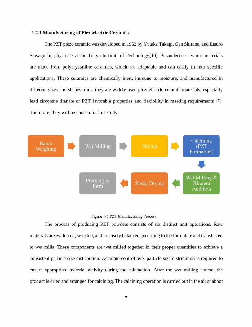
1.2.1 Manufacturing of Piezoelectric Ceramics
The PZT piezo ceramic was developed in 1952 by Yutaka Takagi, Gen Shirane, and Etsuro
Sawaguchi, physicists at the Tokyo Institute of Technology[10]. Piezoelectric ceramic materials
are made from polycrystalline ceramics, which are adaptable and can easily fit into specific
applications. These ceramics are chemically inert, immune to moisture, and manufactured in
different sizes and shapes; thus, they are widely used piezoelectric ceramic materials, especially
lead zirconate titanate or PZT favorable properties and flexibility in meeting requirements [7].
Therefore, they will be chosen for this study.
The process of producing PZT powders consists of six distinct unit operations. Raw
materials are evaluated, selected, and precisely balanced according to the formulate and transferred
to wet mills. These components are wet milled together in their proper quantities to achieve a
consistent particle size distribution. Accurate control over particle size distribution is required to
ensure appropriate material activity during the calcination. After the wet milling course, the
product is dried and arranged for calcining. The calcining operation is carried out in the air at about
Batch Weighing
Wet Milling DryingCalcining
(PZT Formation)
Wet Milling & Bindera Addition
Spray Drying Pressing to
form
Figure 1-5 PZT Manufacturing Process

8
1000°C, where the desired PZT phase is formed. [11] The material is then cooled down, during
which the ceramic becomes ferroelectric, and its unit cells change from cubic to tetragonal
structure. As a result, the unit cells are elongated in one direction, and an electric dipole moment
is generated within the unit cell. The application of a strong D.C. electric field has the effect of
aligning most unit cells parallel to the applied field. Piezoelectric materials can be bonded/glued
to host structures' surfaces or embedded within them [7].

9
1.2.2 Piezoelectric Materials as Energy Harvesters
Energy harvesting or power harvesting is the development by which energy is obtained
from external sources captured, and stored for small, wireless autonomous devices, like those used
in wearable and wireless sensor networks. The external sources as, thermal energy, wind energy,
solar power, salinity gradients, and kinetic energy.[12]
Energy harvesters deliver a small amount of power for electronics with low-energy. The
energy can be stored and used to bias to power electronic devices. With recent advances in wireless
and MEMS technology, energy harvesting is highlighted as the conventional battery alternatives.
Ultra-low-power portable electronics and wireless sensors use conventional batteries as their
power sources. However, battery life is limited and noticeably short contrasted to the working life
of the devices. The recharging or replacement of the battery can be inefficient and not cost-
effective. Therefore, a substantial number of researchers have been focusing on self-powered
portable devices or wireless sensors. Piezoelectric materials are a convenient way to collect energy
from wasted or not useable energy. As mentioned earlier, these materials exhibit electromechanical
coupling; they can convert between strain energy and electrical energy. Several models have been
suggested to quantify the electrical energy that can be generated. Ambrosio et al. [13] proposed a
lead zirconium titanate cantilever as a power generator for an energy harvesting system. The
determination of optimal performance is in terms of power output. Series and parallel are two
different configurations of the piezoelectric element that were studied: l. The piezoelectric system's
maximum output power was 120 mW at the operating frequency of 40 Hz across a resistive load
of 70 kΩ. The excellent power was capable of bias some electronic devices. Cˇeponis et al. [14]
demonstrated numerical and experimental investigation of trapezoidal cantilevers with irregular
cross-sections. Modifications of the cross-section were made to increase strain and improve its

10
distribution in the piezoceramic layer. The numerical analysis indicated a dependency between
strain/stress and the piezoelectric sensor geometry's electrical output. Other significant results
showed that the generated electric power for a geometry altered piezoelectric cantilever is more
than 11.5-times larger than the power obtained from the conventional cantilever. Choi et al. [15]
developed an energy harvesting MEMS device using thin-film PZT to enable self-supportive
sensors. Resonating at certain frequencies of an external vibrational energy source can create
electrical energy via the piezoelectric effect. The effect of the proof mass, beam shape, and
damping on the power generating performance were modeled to provide a guideline for maximum
power harvesting from environmentally available low-frequency vibrations. Sirohi et al. [16]
developed a mechanism based on a galloping piezoelectric bimorph cantilever beam to obtain wind
power. The shaft has a D-shaped cross-section with a rigid, prismatic tip body. Piezoelectric sheets
bonded on the beam transform the strain energy into electrical energy. The power output was noted
to increase rapidly with increasing wind speed. Due to the beam's structural damping, a minimum
wind velocity of 2.5 m/s was necessary to produce power from this device. The highest power
output of 1.14 mW was quantified at a wind velocity of 4.7 m/s. Weinstein. [17] proposed a
cantilevered piezoelectric beam in a heating, ventilation, and air conditioning (HVAC) flow. The
geometry contains a fixed cylinder and a bilayer cantilever with a clamped end on one side, and
the other is free. The fixed cylinder is employed to generate a vortex street. The arranging of small
weights along the fin enables modification of the energy harvested. Power generation of 200 μW
at a flow speed of 2.5 m/s and 3 mW for a 5 m/s was achieved. Power output from this device was
between 100 and 3000 𝜇W for flow speeds in the range of 2–5 m/s. These power outputs are
sufficient to power a wireless sensor node for HVAC monitoring systems or other sensors for smart
building technology. Shen et al. [18] proposed a PZT piezoelectric cantilever with a

11
micromachined Si proof mass for a low-frequency vibration energy harvesting application. The
average power and power densities were 0.32 W and 416 W/cm3. A broadband piezoelectric
energy harvester with an applied restoring force was presented by Rezaei et al [19]. The system
consisted of a cantilever beam bonded with a piezoelectric PZT layer at the top surface and a tip
mass at the free end, which was supported by a spring to model the restoring force. The
piezoelectric harvester was subjected to harmonic base excitation and effects of the PZT layer on
free vibrations, and those of the tip mass and base excitation on the frequency response of the
system were investigated. As expected, the tip mass helped increase the scavenged voltage and
tune the resonance frequency. It was also shown that a pure nonlinear restoring force by the spring
caused the harvester resonance bandwidth and the output voltage to increase as compared to the
energy harvester without the spring.

12
1.2.3 Using Piezoelectric Materials as Flow Rate Sensors
Microelectromechanical system (MEMS) technology has initiated up new avenues in
developing flow sensors for various applications. MEMS devices were first proposed in the 1960s,
following the investigation of silicon and germanium's piezoresistive potential. The investigation
and development in this area have progressively scaled up since the 1980s[20]. MEMS devices
offer small, low-cost, and scalable devices that were not achievable using traditional engineering
methods. Microfabrication technologies have recently been widely employed to fabricate MEMS
sensors for use in a broad range of appliances, such as healthcare, physical activities, safety, and
environmental sensing [21]. Due to these fundamental benefits, MEMS flow sensors are used
broadly in numerous applications such as object detection and navigation on autonomous
underwater vehicles (AUV) [22], flow measurement in biomedical surgery, diagnostic devices,
chemistry and therapeutic areas[23], liquid dispensing systems [24], and gas monitoring systems
[25], [26]. MEMS flow sensors have been developed using silicon and polymer materials and
applying various sensing and structural designs. The most common sensing methods are thermal
[27], [28], torque[29], [30] and drag force based [31] flow sensing. Liu et al. [32] used the Lead
Zirconium titanite (PZT) microcantilever as an airflow sensor for wind-driven energy harvesting.
They obtained a flow sensing sensitivity of 9 mV/ (m/s). It generated 18.1 mV and 3.3 nW for a
stream velocity of 15.6 m/s Resister (load) of a 100 kΩ. Seo et al. [33] proposed a self-resonant
flow sensor centered on a resonant frequency shift due to turbulence-induced vibrations. The
reaction of the cantilever beam was modulated with its resonant frequency. The flow drag force
produced a mechanical strain on the cantilever beam; then, the modulated frequency shifted. The
device is a hanging crossflow stalk, which can amplify the vibration by order of magnitude. The
experimental demonstration indicated a peak output power of 0.6 mW and a max power density of

13
2 mW/cm3. Yu-Hsiang et al.[34] has developed a MEMS-based airflow sensor featuring a free-
standing micro-cantilever structure. In the sensing operation, the airflow velocity is detected by
measuring the difference in resistance of a piezoelectric layer placed on a cantilever beam as the
beam deforms under the passing airflow effect. The experimental outcomes indicate that the flow
sensor has a high sensitivity (0.0284 Ω/ms-1), a high-velocity measurement limit (45 ms-1), and
rapid response time (0.53 s). Qi Li. et al. [35] proposed measuring the flow velocity of fluid without
affecting its motion state; this method was based on polyvinylidene fluoride (PVDF) piezoelectric
film sensor. The piezoelectric principle of a PVDF film was analyzed. The turbulence noise of a
flat-panel model simulated. A flow velocity measurement system with a PVDF film as the sensing
component built the piezoelectric response of the PVDF sensor under wind excitation was
measured. The proposed method was shown to be dependable and effective
Flow sensors are necessary to measure the rate and direction of liquid or gas flow in various
applications. Sensors include the determination of flow patterns [36], measurement of wall shear
stress [37], viscosity, and density measurements [38] in different systems. During the past decades,
numerous sensing devices have been developed and become commercially available for flow
measurement. It is understood that the flow measurement may be influenced by the velocity,
pressure, temperature, or chemical content of the systems [39]. Therefore, flow sensing devices
are typically centered on the direct detection of volume, mass, velocity, or combination by
measuring various physical variables [40], [41].
In recent years, industrial and academic investigation groups have focused their attention
on the challenges and limitations of employing piezoelectric materials as energy harvesting tools.
For example, Kuchle and Love [42] and Sarker et al.[43] used thermoelectric and pyroelectric
sensors to wirelessly detect the temperature inside of a power generation unit at places where

14
thermocouples unreachable. This technology would allow for real-time health monitoring and
material temperatures in areas such as the unit's turbomachinery.
Other parameters, such as velocity, also provide insight into turbomachinery or flow rate
behaviors within a system. The velocity parameter is desirable if the sensor can detect rapid flow
or pressure measurement changes. Piezoelectrics have been operated frequently in the past for
pressure measurements. [44] However, flow velocity measurements using the same material are
not commonly used for the macro scale. The focus was on micro-scale for medical, industrial, and
environmental applications. Ejeian et al. [45] presented the work done on the
Microelectromechanical system's design and development (MEMS)- based flow sensors in recent
years. However, macroscale and large flow rate measurements using similar sensors are not well
documented in the literature. In the energy industry, piezoelectric materials have opened many
research interests. Many studies have been utilized piezoelectric ceramics as energy harvesting
devices [17], [32], [46]–[49]. However, the produced signal can also be analyzed to identify flow
characteristics such as velocity, typically using soft PZT ceramics. These devices are subject to
fluid flow that cause stress and bend on the geometry that the piezoelectric attached. In all cases,
this motion is converted to electricity. Earlier designs that involve piezoelectric include cantilever
beams that vibrate due to vortices produced by fluid flows, such as in a Vortex flowmeter [50].
Many of these sensors in this arrangement are also used to harvest energy. [8], [51]

15
1.3 Piezoelectric Constitutive Equations
In this section, the equations which illustrate the electromechanical properties of
piezoelectric materials will be described. They are based on the IEEE standard for piezoelectricity
widely accepted as a description of piezoelectric material properties. The IEEE standard is made
based on the assumption that piezoelectric materials are linear. It turns out that piezoelectric
materials have a linear profile at low electric fields and low mechanical stress levels. However,
they may show substantial nonlinearity if operated under a high electric field or high mechanical
stress level. For the most part, the piezoelectric transducers are being used at low electric fields
and small mechanical stress. Electricity produces a charge on the material's surface when a poled
piezoelectric ceramic is mechanically strained. This property is described as the "direct
piezoelectric effect." Moreover, it is the basis upon which the piezoelectric materials are used as
sensors. Furthermore, if electrodes are attached to the material's surfaces, the generated electric
charge can be collected and used.

16
The fundamental equations describing piezoelectric properties are based on the assumption
that the transducer's total strain is the sum of mechanical strain produced by the mechanical stress
and the controllable actuation strain caused by the applied electric voltage.[8] The axes are
identified by numerals rather than letters. Moreover, Figure 1-6 shows the schematic diagram of
the piezoelectric transducer. The illustrating electromechanical equations for a linear piezoelectric
material can be written as
휀𝑖 = 𝑆𝑖𝑗𝐷𝜎𝑗 + 𝑑𝑚𝑖𝐸𝑚
1.1
𝐷𝑚 = 𝑑𝑚𝑖𝜎𝑖 + 𝜉𝑖𝑘𝜎 𝐸𝑘 1.2
The indexes 𝑖, 𝑗 = 1, 2, . . . , 6 and 𝑚, 𝑘 = 1, 2, 3 relate to different directions within the
material coordinate system; the equations can be re-written in the following form, which is often
used for applications that involve sensing:
휀𝑖 = 𝑆𝑖𝑗𝐷𝜎𝑗 + 𝑔𝑚𝑖𝐷𝑚
1.3
Figure 1-6 Schematic diagram of a piezoelectric transducer

17
𝐷𝑚 = 𝑑𝑚𝑖𝜎𝑖 + 𝛽𝑖𝑘𝜎𝐷𝑘 1.4
Where:
𝜎 : Stress vector (N/m2)
휀 : Strain vector (m/m)
𝐸 : Vector of the applied electric field (V/m)
𝜉 : Permittivity (F/m)
𝑑 : Matrix of piezoelectric strain constants (m/V)
𝑆 : Matrix of compliance coefficients (m2/N)
𝐷 : .Vector of electric displacement (C/m2)
𝑔 : Matrix of piezoelectric constants (m2/C)
𝛽 : Impermittivity component (m/F)
Furthermore, the superscripts 𝐷, 𝐸, and 𝜎 represent measurements taken at constant electric
displacement, constant electric field, and constant stress. In addition, equations (1.1) and (1.3)
express the converse piezoelectric effect, which explains when the device is operated as an
actuator. Alternatively, Equations (1.2) and (1.4) express the direct piezoelectric effect, which
deals with when the transducer is being utilized as a sensor. It should be noted that relations
between applied electric fields and the resultant responses depend upon the ceramic's piezoelectric
properties, the piece's geometry, and the direction of electrical excitation. The properties of
piezoceramic change as a function of both strain and temperature. It should be known that the data
commonly presented represents values measured at low levels of approximately 20°C.

18
1.4 Piezoelectric Coefficients
Piezoelectric coefficients relating to input parameters to output parameters use double
subscripts. The first subscript indicates the electric field 𝐸 or dielectric displacement 𝐷 direction,
and the second subscript describes the direction of mechanical stress 𝑇 or strain 𝑆.
1.4.1 Mechanical Piezoelectric Constant
The piezoelectric coefficient 𝑑𝑖𝑗 The ratio of the strain in the 𝑗 − 𝑎𝑥𝑖s to the electric field
applied along the 𝑖 − 𝑎𝑥𝑖𝑠, when all external stresses are held constant.
Figure 1-9 shows that V's voltage is applied to a piezoelectric transducer, polarized in
direction 3. This voltage generates the electric field as in equation (1.5)
𝐸3 =
𝑉
𝑡
1.5
Which strains the transducer. In particular
휀1 =
∆𝑙
𝑙
1.6
In which
Figure 1-7 A piezoelectric transducer arrangement for d31 measurement

19
∆𝑙 =
𝑑31 𝑉 𝑙
𝑡
1.7
The piezoelectric constant 𝑑31 is usually a negative number; this is because the application
of a positive electric field will generate a positive strain in direction 3.
Another interpretation of 𝑑𝑖𝑗; The proportion of short circuit charge per unit area flowing
between connected electrodes perpendicular to the 𝑗 direction to the stress applied in the 𝑖 direction,
once a force 𝐹 is applied to the transducer in the 3 direction, generates the stress flowing through
the short circuit.
𝜎3 =
𝐹
𝑙 𝑤
1.8
which results in the electric charge
𝑞 = 𝑑33𝐹 1.9
If stress is operated equally in 1, 2, and 3 directions, and the electrodes are perpendicular
to axis 3, the resultant short-circuit charge (per unit area), divided by the applied stressed, is
denoted by 𝑑𝑝.
1.4.2 Electrical Piezoelectric Constant
The piezoelectric constant 𝑔𝑖𝑗 signifies the electric field established along the i-axis when
the material is stressed along the j-axis. Therefore, results in the voltage
𝑉 =
𝑔31 𝐹
𝑤
1.10
Another interpretation of 𝑔𝑖𝑗 is the ratio of strain established along the j-axis to the charge (per
unit area) deposited on electrodes perpendicular to the i-axis. Therefore, if an electric charge of 𝑄
is deposited on the surface electrodes, the thickness of the piezoelectric element will change by

20
∆𝑙 =
𝑔31𝑄
𝑤
1.11
1.4.3 Elastic Compliance Constant
The elastic compliance constant 𝑆𝑖𝑗 is the ratio of the strain in 𝑖 − 𝑑𝑖𝑟𝑒𝑐𝑡𝑖𝑜𝑛 to the stress
in the 𝑗 − 𝑑𝑖𝑟𝑒𝑐𝑡𝑖𝑜𝑛 -given that there is no change of stress along with the other two directions.
Direct strains and stresses are conveyed by indices 1 to 3. Shear strains and stresses are conveyed
by indices 4 to 6. Subsequently, 𝑆12 denotes the direct strain in the 1 − 𝑎𝑥𝑖𝑠 when the device is
stressed along the 2 − 𝑎𝑥𝑖𝑠, and stresses along with directions 1 and 3 are unchanged. Similarly,
𝑆44 refers to the shear strain around the 2 − 𝑎𝑥𝑖𝑠 due to the shear stress around the same axis.
A superscript "𝐸" is used to state that the elastic compliance 𝑆𝑖𝑗𝐸 is measured with the
electrodes short-circuited. Likewise, the superscript "𝐷" in 𝑆𝑖𝑗𝐷 conveys that the measurements were
taken when the electrodes were left open-circuited. Mechanical stress outcomes in an electrical
response that can increase the resultant strain. Therefore, it is natural to expect 𝑆𝑖𝑗𝐸 to be smaller
than 𝑆𝑖𝑗𝐷 . That is, a short-circuited piezo has a lesser Young's modulus of elasticity than when it is
open-circuited.
1.4.4 Dielectric Coefficient
The dielectric coefficient 𝑒𝑖𝑗 defines the charge per unit area in the 𝑖 − 𝑎𝑥𝑖𝑠 due to an
electric field applied in the 𝑗 − 𝑎𝑥𝑖𝑠. In general piezoelectric materials, a field applied along with
the 𝑗 − 𝑎𝑥𝑖𝑠 cause electric displacement only in that direction. The relative dielectric constant,
identified as the ratio of the absolute permittivity of the material by the permittivity of free space,
is symbolized by 𝐾. The superscript 𝜎 in 𝑒11𝜎 refers to the permittivity for a field applied in the
1 − 𝑑𝑖𝑟𝑒𝑐𝑡𝑖𝑜𝑛, when the material is not restrained.

21
1.4.5 Piezoelectric Coupling Coefficient
The piezoelectric coefficient 𝑘𝑖𝑗 signifies the ability of a piezoceramic material to
transform electrical energy into mechanical energy and vice versa. This conversion of energy
between mechanical and electrical domains is employed in both sensors and actuators made from
piezoelectric materials. The 𝑖𝑗 index indicates that the stress or strain is in the 𝑑𝑖𝑟𝑒𝑐𝑡𝑖𝑜𝑛 𝑗, and the
electrodes are perpendicular to the 𝑖 − 𝑎𝑥𝑖𝑠. For instance, if a piezoceramic is mechanically
strained in 𝑑𝑖𝑟𝑒𝑐𝑡𝑖𝑜𝑛 1, as a result of electrical energy input in 𝑑𝑖𝑟𝑒𝑐𝑡𝑖𝑜𝑛 3, while the device is
under no exterior stress, then the ratio of stored mechanical energy to the affected electrical energy
is denoted as 𝑘312 .
There are several ways that 𝑘𝑖𝑗 can be measured. One option is to apply a force to the
piezoelectric element while keeping its terminals open-circuited. The piezoelectric device will
deflect. This deflection ∆𝑧, can be evaluated, and the mechanical work performed by the applied
force 𝐹 can be determined
𝑊𝑀 =
𝐹∆𝑧2
1.12
Due to the piezoelectric effect, electric charges will be collected on the transducer's
electrodes transfer to the electrical energy
𝑊𝐸 =𝑄2
2𝐶𝑝
1.13
Which is stored in the piezoelectric capacitor. Therefore,
𝑘33 = √𝑊𝐸
𝑊𝑀=
𝑄
√𝐹 ∆𝑧 𝐶𝑝
1.14
The pairing coefficient can be written in terms of other piezoelectric constants. In particular

22
𝑘𝑖𝑗2 =
𝑑𝑖𝑗2
𝑆𝑖𝑗𝐸𝑒𝑖𝑗
𝜎 = 𝑔𝑖𝑗𝑑𝑖𝑗𝐸𝑝 1.15
Where 𝐸𝑝 is Young's modulus of elasticity of the piezoelectric material.
When a force is applied to a piezoelectric transducer, depending on whether the device is
open-circuited or short-circuited, one should expect to observe different stiffnesses. In particular,
if the electrodes are short-circuited, the device will appear to be "less stiff" because, upon applying
a force, the electric charges of opposite polarities collected on the electrodes terminate each other.
Consequently, no electrical energy can be stored in the piezoelectric capacitor. Denoting short-
circuit stiffness and open-circuit respectively as 𝐾𝑠𝑐 and 𝐾𝑜𝑐, it can be proved that [8]
𝐾𝑜𝑐𝐾𝑠𝑐
=1
1 − 𝑘2
1.16
23
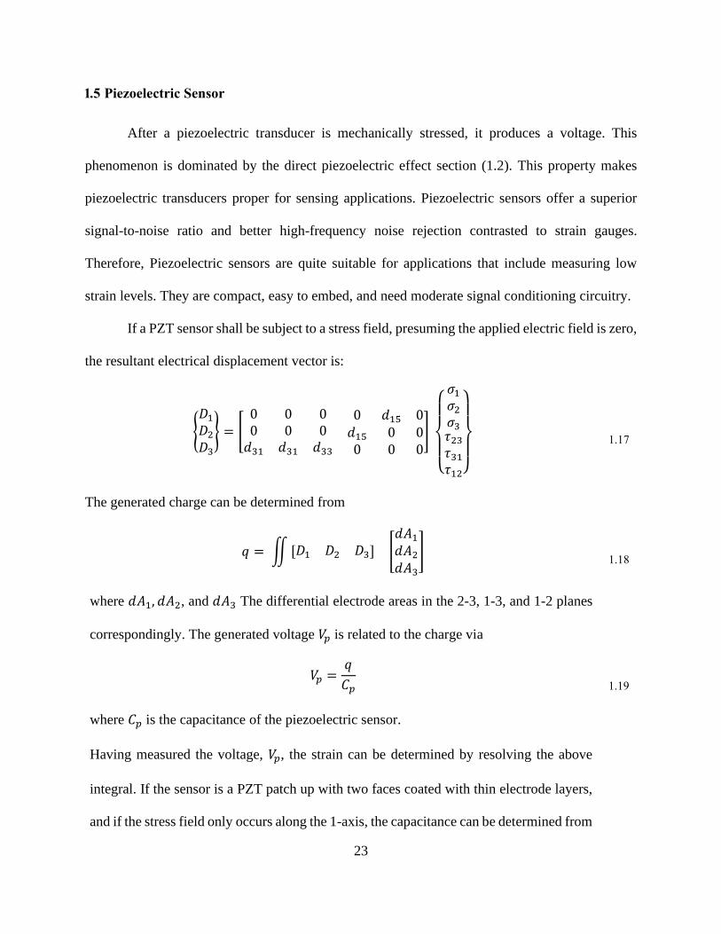
1.5 Piezoelectric Sensor
After a piezoelectric transducer is mechanically stressed, it produces a voltage. This
phenomenon is dominated by the direct piezoelectric effect section (1.2). This property makes
piezoelectric transducers proper for sensing applications. Piezoelectric sensors offer a superior
signal-to-noise ratio and better high-frequency noise rejection contrasted to strain gauges.
Therefore, Piezoelectric sensors are quite suitable for applications that include measuring low
strain levels. They are compact, easy to embed, and need moderate signal conditioning circuitry.
If a PZT sensor shall be subject to a stress field, presuming the applied electric field is zero,
the resultant electrical displacement vector is:
𝐷1𝐷2𝐷3
= [0 0 00 0 0𝑑31 𝑑31 𝑑33
0 𝑑15 0𝑑15 0 00 0 0
]
𝜎1𝜎2𝜎3𝜏23𝜏31𝜏12
1.17
The generated charge can be determined from
𝑞 = ∬[𝐷1 𝐷2 𝐷3] [
𝑑𝐴1𝑑𝐴2𝑑𝐴3
] 1.18
where 𝑑𝐴1, 𝑑𝐴2, and 𝑑𝐴3 The differential electrode areas in the 2-3, 1-3, and 1-2 planes
correspondingly. The generated voltage 𝑉𝑝 is related to the charge via
𝑉𝑝 =𝑞
𝐶𝑝
1.19
where 𝐶𝑝 is the capacitance of the piezoelectric sensor.
Having measured the voltage, 𝑉𝑝, the strain can be determined by resolving the above
integral. If the sensor is a PZT patch up with two faces coated with thin electrode layers,
and if the stress field only occurs along the 1-axis, the capacitance can be determined from

24
𝐶𝑝 =
𝑙 𝑤 𝑒33𝜎
𝑡
1.20
Assuming the resultant strain is along the 1-axis, the sensor voltage is found to be
𝑉𝑠 =
𝑑31 𝐸𝑝 𝑤
𝐶𝑝 ∫휀1 𝑑𝑥𝑙
1.21
where 𝐸𝑝 is Young's modulus of the sensor, and 휀1 is averaged over the sensor's length.
The strain can then be calculated from
휀1 =
𝐶𝑝𝑉𝑠
𝑑31 𝐸𝑝 𝑙 𝑤
1.22
In deriving the above equations (1.17) (1.18) (1.19) (1.20) (1.21) and (1.22), the primary
assumption was that the sensor was strained along 1-axis only. If this assumption is
violated, which is frequently the case, then equation (1.22) should be modified to
휀1 =
𝐶𝑝𝑉𝑠(1 − 𝜈)𝑑31 𝐸𝑝 𝑙 𝑤
1.23
Where 𝜈 is the Poisson's ratio. [8]
The listed equations before can be summarized in Table 1-1
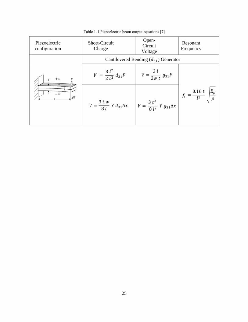
25
Table 1-1 Piezoelectric beam output equations [7]
Piezoelectric
configuration
Short-Circuit
Charge
Open-
Circuit
Voltage
Resonant
Frequency
Cantilevered Bending (𝑑31) Generator
𝑉 = 3 𝑙2
2 𝑡2 𝑑31𝐹 𝑉 =
3 𝑙
2𝑤 𝑡 𝑔31𝐹
𝑓𝑟 =0.16 𝑡
𝑙2 √𝐸𝑝
𝜌
𝑉 =3 𝑡 𝑤
8 𝑙 𝑌 𝑑31∆𝑥 𝑉 =
3 𝑡2
8 𝑙2 𝑌 𝑔31∆𝑥
26
1.6 Dynamic Input Forces or Displacements
Piezo is much more responsive to dynamic applications. Where dynamic inputs have two
categories, either be pulsed or continuous. Pulsed input or short duration, transient force, creep,
and electrical leakage issues are minor since there is insufficient time for their behavior to take
place. Continuously alternating input forces are when the generator is excited by an oscillating
force.
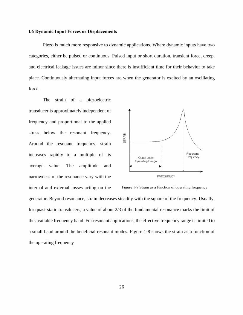
The strain of a piezoelectric
transducer is approximately independent of
frequency and proportional to the applied
stress below the resonant frequency.
Around the resonant frequency, strain
increases rapidly to a multiple of its
average value. The amplitude and
narrowness of the resonance vary with the
internal and external losses acting on the
generator. Beyond resonance, strain decreases steadily with the square of the frequency. Usually,
for quasi-static transducers, a value of about 2/3 of the fundamental resonance marks the limit of
the available frequency band. For resonant applications, the effective frequency range is limited to
a small band around the beneficial resonant modes. Figure 1-8 shows the strain as a function of
the operating frequency
Figure 1-8 Strain as a function of operating frequency

27
1.7 Electrical Outputs
Piezoelectric generators are
typically specified in terms of their short-
circuit charge and open-circuit voltage.
Short-circuit charge, 𝑄𝑠, refers to the total
charge established, at the maximum
recommended stress level, when the charge
is entirely free to travel from one electrode
to the other and is not asked to build up any
voltage. Open-circuit voltage, 𝑉𝑜 Refers to the voltage created, at the maximum proposed stress
level, when the charge is prohibited from traveling from one electrode to another. The charge is
maximum when the voltage is zero, and the voltage is at a maximum when the charge transfer is
zero. Every other simultaneous charge and voltage level value is governed by a line drawn between
these points on a voltage against the charge line, shown in Figure 1-9. Generally, a piezo generator
must transfer a specified amount of charge and supply a specific voltage, which defines its
operating point on the voltage vs. charge line. Work is amplified when the charge moved permits
one half the open-circuit voltage to be developed, which occurs when the charge equals one half
the short-circuit charge. [7]
Figure 1-9 The voltage versus charge diagram for a
piezoelectric generator element

28
1.8 Signal to Noise Ratio
The Signal-Noise Ratio (SNR) is how strong the signal is compared to the noise. Some
amount of noise contaminates every signal. This noise is added to the signal, and if it is too much,
it will make the signal undetectable. Therefore, it is desired to have a signal-to-noise ratio as high
as possible. The Signal-Noise Ratio is the ratio between the signal power and the noise power, and
it can be calculated as in equation 1.24
𝑆𝑁𝑅 =
𝑃𝑠𝑖𝑔𝑛𝑎𝑙
𝑃𝑛𝑜𝑖𝑠𝑒
1.24
The typical power of an AC signal is defined in physics as the average of voltage times
current.
𝑃 = 𝑉𝑅𝑀𝑆 𝐼𝑅𝑀𝑆 1.25
For resistive circuits, where voltage and current are in phase, this power is equivalent to
the product of the root mean square (RMS) voltage and current:
𝑃 =
𝑉𝑅𝑀𝑆2
𝑅 1.26
The same resister, R, was used in collecting the signal and the noise for this project. As a
reason, we can calculate the SNR from:
𝑆𝑁𝑅 =
𝑉𝑅𝑀𝑆 𝑆𝑖𝑔𝑛𝑎𝑙2
𝑉𝑅𝑀𝑆 𝑁𝑜𝑖𝑠𝑒2
1.27
The SNR usually standardized by converting it to dB
𝑆𝑁𝑅𝑑𝐵 = 10 log10(𝑆𝑁𝑅) = 20 log10 (
𝑉𝑅𝑀𝑆 𝑆𝑖𝑔𝑛𝑎𝑙
𝑉𝑅𝑀𝑆 𝑁𝑜𝑖𝑠𝑒)
1.28
This study defined the noise as the signal collected when no flow was passing in the setups,
and it is assumed the noise signal includes all the external and internal noise.

29
1.9 Surge and Stall
Surge is a global instability in a centrifugal compressor's flow resulting in a complete
failure and reversal of flow through the compressor. Surge happens just below the minimum flow
that the compressor can maintain against the existing suction to discharge pressure rise (head).
When a surge occurs, both flow rate and charge decrease rapidly, and gas flows backward within
the compressor. Surge is a source of large dynamic forces applied to the compressor elements and,
hence, a flow phenomenon that must be avoided. Surge avoidance is essential for pipeline
compressors and is typically achieved by recycling gas around the compressor to maintain a flow
of no less than the surge control flow rate. External measurements of head and speed generally are
used to retain the control surge line's operating flow rate. Although the operating point can be
maintained by recycling flow, recycling flow around compressors wastes energy and can be
extremely inefficient. If the physical approach of surge can be detected, then centrifugal
compressors can be operated closer to surge without recycling as much flow. The current surge
avoidance and control methods resulted in recycling valves being used extensively and opened
well before the compressor is in danger of reaching the surge. The purpose of the current direct
surge control effort, using measurements that are internal to the compressor, is to reduce surge
margins, use less recycle flow during operations, and reduce wasted fuel and operating costs.[52].
Compressor surge can be categorized into mild surge, deep surge, and. While the one without
reverse flows generally termed mild surge, a Compressor surge with negative mass flow rates is
considered a deep surge [53]. On a performance map, the steady operating range of a typical
performance map for a pipeline centrifugal compressor shows the pressure increase as head rise as
a function of inlet volumetric flow for a compressor range speeds shown in Figure 1-10.[54] This
compressor map indicates that there are limits on the operating range of such a compressor. The
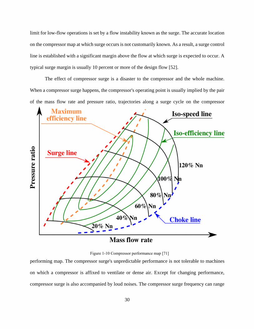
30
limit for low-flow operations is set by a flow instability known as the surge. The accurate location
on the compressor map at which surge occurs is not customarily known. As a result, a surge control
line is established with a significant margin above the flow at which surge is expected to occur. A
typical surge margin is usually 10 percent or more of the design flow [52].
The effect of compressor surge is a disaster to the compressor and the whole machine.
When a compressor surge happens, the compressor's operating point is usually implied by the pair
of the mass flow rate and pressure ratio, trajectories along a surge cycle on the compressor
performing map. The compressor surge's unpredictable performance is not tolerable to machines
on which a compressor is affixed to ventilate or dense air. Except for changing performance,
compressor surge is also accompanied by loud noises. The compressor surge frequency can range
Figure 1-10 Compressor performance map [71]

31
from a few to dozens of Hertz, depending on the compression system's configuration. [55]
Although Helmholtz resonance frequency is often employed to characterize mild surges'
instability, it was observed that Helmholtz oscillation did not trigger a compressor surge in some
cases [56]. Another effect of compressor surge is on a solid structure. Violent compressor surge
flows repeatedly hit blades in the compressor, causing blade fatigue or even mechanical failure.
While a fully established compressor surge is axisymmetric, its initial phase is not necessarily
axisymmetric. In general, In most low-speed and low-pressure cases, a rotating stall comes before
compressor surge [57], [58]. However, a general cause-effect relation between rotational stall and
compressor surge has not been determined yet. [56] On a compressor's constant speed line, the
mass flow rate decreases as the compressor's pressure increases. Inner flows of the compressor are
in a substantial harmful pressure gradient, which tends to disrupt the flow and cause flow
separation. A wholly developed compressor surge can be modeled as a one-dimensional global
instability of a compression system that typically consists of inlet ducts, compressors, exit ducts,
gas reservoirs, and throttle valves.[59], [60] A cycle of compressor surge can be divided into
several phases, [61] If the throttle valve is turned to be a tiny opening, the gas reservoir would
have a positive net flux. The reservoir pressure keeps increasing and then exceeds the compressor
exit pressure, resulting in a harmful pressure gradient in exit ducts. This harmful pressure gradient
naturally decelerates flows in the entire system and lowers the mass flow rate. The gradient of a
constant speed line near the surge line is typically zero or even positive, which indicates that the
compressor cannot deliver a much higher pressure as lowering the mass flow rate. Hence, the
adverse pressure gradient could not be suppressed by the compressor. The system would rapidly
involve an overshoot of adverse pressure gradient, dramatically reducing the mass flow rate or
even cause flows to reverse. On the other hand, the reservoir's pressure would gradually drop due

32
to less flux delivered by the compressor, hence rebuilding a favorable pressure gradient in exit
ducts. After that, the mass flow rate would be recovered, and the compressor is back to work on a
constant speed line again, which would eventually trigger the next surge cycle. Therefore,
compressor surge is a process that keeps breaking the flow path of a compression system down
and rebuilding it [62]
A compressor will simply steadily pump air up to a certain pressure ratio. Further, from
this value, the flow will break down and become unbalanced. This unsteady flow occurs at the
surge line on a compressor map. The engine is designed to keep the compressor operating a little
distance below the surge pressure ratio on the compressor map's operating line. The space between
the two lines is the surge margin on a compressor map. Several things can occur during the engine's
operation to lower the surge pressure ratio or raise the operating pressure ratio. When the two
coincide, there is no longer any surge margin, and a compressor stage can stall, or the complete
compressor can surge as explained in the preceding sections. These pressure ratios typically
change when the power plant load changes and is more severe in the combined cycle.
Surge and stall are one of the operational challenges in Solid Oxide Fuel Cell / Gas Turbine
(SOFC/GT) hybrid systems. These situations, which start on the turbine side, leads to the failure
of the entire cycle. That can be expensive to maintain and increase the safety factors on operation
conditions and lower the efficiency. These conditions make it is hard to move forward on
commercializing the hybrid system. An advanced control system supported with accurate and fast
response sensors and instruments can minimize these effects and increase its overall efficiency. A
possible solution is to examine the flow rate at the compressor discharge and implement a
piezoelectric flow sensor to identify when surge and stall will occur and stop the process before a
catastrophic situation happens.

33
1.10 Practical Relevance
Improving the Hybrid Performance (HYPER) system's overall efficiency -and other energy
systems - may be achievable by integrating a smart sensor, such as the one proposed. The
compressor surge is destructible for the turbomachinery and extremely harmful for the fragile
SOFC electrolyte. Hence, compressor dynamics need to be controlled. A safe emergency system
needs to be implemented on this power plant to avoid surge during sudden maneuvers such as
emergency shut down. The challenges illustrated and discussed apply to any gas turbine-based
hybrid system. A significant volume is added between compressor and expander, such as
concentrated solar gas turbine hybrid plants, integrated thermal-energy-storage/gas turbine
systems, and integrated geothermal/gas turbine hybrids.
The compressor surge may be detected and avoided before causing damage if the
compressor dynamics are controlled faster than existing hardware allows. The HYPER facility's
operation may be improved, and compressor stall is mitigated during transient operation periods
if rapidly responding measurement sensors are integrated. It is investigating the use of
piezoelectric sensors for a variety of power generation monitoring applications. Recent work has
demonstrated a sensor's ability to be used in a wireless configuration to measure pressure change
using a lower temperature material, Lead-Zirconate Titanate (PZT). Developing a sensor that is
efficient in measuring immediate pressure measurements would prevent these tasks. The sensor
could be positioned on the surface of the measurement point of interest. Once in place, the sensor
will respond when exposed to a pressure change with time. The current produced by the sensor
can be calibrated to represent changes in pressure or wind and control the system.

34
1.11 Objective
As mentioned in the previous section, piezoelectric materials are used in the literature,
primarily energy harvesting devices to recover waste energy. Most studies present a cantilever
beam variation in a flowing stream to recover kinetic energy and convert it to electrical energy.
Typically, this is done for flow rates in the range of 3.97 × 10⁻² 𝑡𝑜 1.34 × 10⁻¹ m3/s, which is
very low for industrial purposes. This dissertation investigates the sensor's signal output to indicate
the system's flow instead of energy harvesting methods. If the system can sense a change in the
flow, particularly at a rapid (5ms) sample rate, it would have many energy industry applications
based on the properties and behavior.
One of the applications that this sensor may be used is in the HYPER facility at the National
Energy Technology Laboratory. If the flow sensor can measure flows accurately, it may assist in
the mitigation of compressor stall during transient operational periods. Hence, this dissertation
investigates:
1) The feasibility of using a piezoelectric material as a flow measuring device for internal
flows
2) An investigation of the effect of piezoelectric dimensions on the output voltage signal
produced by the flow
Experimental setups were developed to complete the tasks for this project. The design of the
experimental setups is based on the listed criteria:

35
1) Design a system that can produce repeatable internal flow velocities and control
airflow velocities from 0-15 m/s.
2) Design a system with multiple fluid velocity profiles at room temperature and
pressure
3) Integrate the sensor into the NETL facility and have the capability to test various
geometries

36
Chapter 2: Methodology
2.1 Theory
This project has divided into two phases to achieve the tasks above, where:
• Phase 1: Design a system that can produce repeatable flow velocities and control airflow
velocities from 0-15 m/s. Test the sensor when exposed to multiple fluid velocities at room
temperature and pressure
• Phase 2: Test the sensors with different geometry (area, thickness, aspect ratio) when exposed
to multiple velocities.
2.1.1 Phase I: Piezoelectric as a Flow Rate Sensor and velocity profile.
2.1.1.1 Piezoelectric as flow rate:
A simple design of setups and sensing element is employed as the focus of this project is
to study the sensing element geometry.
Figure 2-1 Schematic of the piezo sensor as cantilever beam

37
The flow sensor's design is presented in Figure 2-1; the airflow applies a beam load. The
piezoelectric ceramic is fixed on one end, and the other end is free, making the system a cantilever
beam. Therefore, the magnitude of the voltage produced by a piezoelectric material is related to
stress or strain, as the equations presented in Chapter 1. Many forces may impact the stress field.
However, based on the experimental setup, it is hypothesized that the major contributor to internal
stress is the drag force. Equation (2.1) shows the general formula for the drag force.
𝐹𝑑 =
1
2 𝜌 𝐴 𝐶𝐷𝑣
2 2.1
Where
𝐹𝐷 ∶ Drag force, [N]
ρ is the fluid density of air at room temperature and pressure, [kg/m3]
𝐴 : The surface contact area between the fluid and body, [m2]
𝐶𝐷 : The drag coefficient
𝑣 : The average velocity of the fluid acting on the surface of the body. [m/s]
The drag coefficient was estimated based on the flow perpendicular to a flat plate [63].
The piezoelectric ceramic has its electrodes on the faces that are normal to 𝑧𝑦 plane (3 −
𝑑𝑖𝑟𝑒𝑐𝑡𝑖𝑜𝑛). The voltage generated is between the electrodes. To get the voltage in 3 − 𝑑𝑖𝑟𝑒𝑐𝑡𝑖𝑜𝑛,
we need the electric displacement in 3 − 𝑑𝑖𝑟𝑒𝑐𝑡𝑖𝑜𝑛, and since the strain and stress in the beam are
assumed to be only on 1 − 𝑑𝑖𝑟𝑒𝑐𝑡𝑖𝑜𝑛, there is no external electric field applied to the beam. The
coupling of force and voltage generated in the PZT relates to the flow field's velocity and
volumetric or mass flow rate.

38
2.1.1.2 Velocity and duct shape effect
Inside the rectangular and circular duct, the velocity of the flow changes depending on the
height. Therefore, the drag force will vary depending on the velocity profile. It will be calculated
for phase 1 & 2 as the average velocity from the velocity profile to impact the apparatus.
Figure 2-2 presents the velocity profile in a rectangular duct. The velocity profile is not
homogenous. The maximum velocity occurs in the duct center, while the velocity near the wall,
the velocity drops to zero. This profile is for a free stream with no obstruction for fully developed
flow.
Figure 2-2 Velocity profile in a rectangular duct [72]
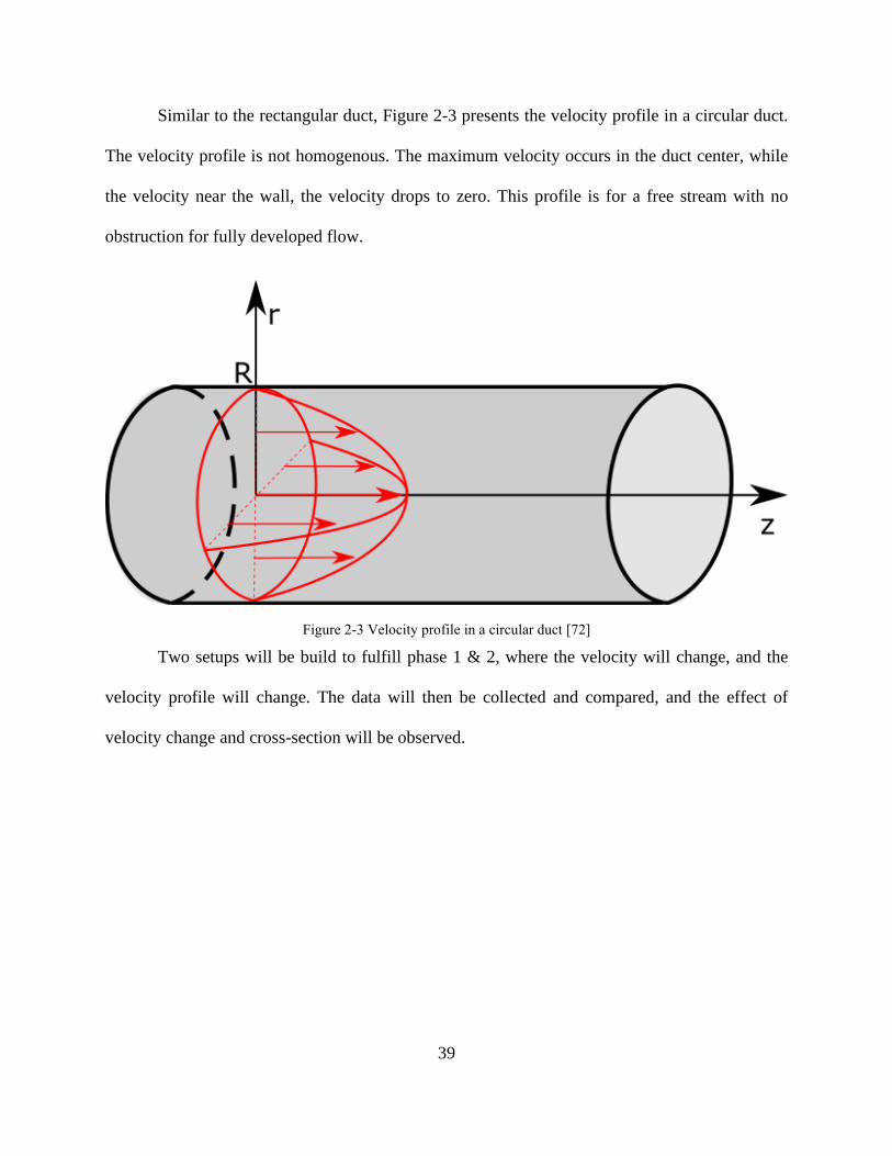
39
Similar to the rectangular duct, Figure 2-3 presents the velocity profile in a circular duct.
The velocity profile is not homogenous. The maximum velocity occurs in the duct center, while
the velocity near the wall, the velocity drops to zero. This profile is for a free stream with no
obstruction for fully developed flow.
Two setups will be build to fulfill phase 1 & 2, where the velocity will change, and the
velocity profile will change. The data will then be collected and compared, and the effect of
velocity change and cross-section will be observed.
Figure 2-3 Velocity profile in a circular duct [72]

40
2.1.2 Phase II: Geometrical effect and Empirical Equation
Table 1-1summarize the equations used for the Piezoelectric cantilever beam generator,
and equation 2.2, 2.3 shows the relationship between the independent variables and voltage, and
drag force
𝑉 =3 𝑙
2𝑤 𝑡 𝑔31𝐹
2.2
𝐹𝑑 =1
2 𝜌 𝐴 𝐶𝐷𝑣
2 2.3
. Equation 2.4 is the combination of the previous equations.
𝑉 =
3
4 𝐶𝐷 . 𝜌. 𝑔31.
𝑙
𝑤.𝐴
𝑡. 𝑣2
2.4
However, when the equation was applied, the result was very different from the
experimental data. One assumption for these differences is the dynamic load (vibration) of the
flow, while the equation considers static load. Therefore, a correction factor is needed to adjust
this offset. Using Buckingham Pi-theorem [64], we can determine the factor. The assumption is
that the output voltage is a function of the variables shown below:
𝑉~𝑓(𝐶𝐷 , 𝜌, 𝑔31,
𝑙
𝑤,𝐴
𝑡, 𝑣) 2.5
Where
𝑉 : The voltage output [V]
𝐶𝐷: The drag coefficient [1]
𝜌 : the density of the fluid [kg/m3]
𝑔31 : The electrical piezoelectric constant [V.m/N]
𝑙
𝑤 : The aspect ratio [m/m]
𝐴
𝑡 : The thickness in [m2/m]

41
𝑣 : The free stream velocity [m/s]
In this phase, the test specimens have the same cross-section area (rectangular), and they
are made from the same material. Also, the working fluid to test the specimens is constant (Air).
Therefore 𝐶𝐷 , 𝜌, 𝑔31 considered constant and equation 2.5 become the following
𝑉~ 𝑓 (
𝑙
𝑤,𝐴
𝑡, 𝑣)
2.6
This equation can be described as
𝑉 = 𝑎. (
𝑙
𝑤)𝑏
. (𝐴
𝑡)𝑐
. 𝑣𝑑 2.7
These coefficients (a,b,c,d) can be estimated using multi-linear regression.
2.1.2.1 Multi-linear regression
linear regression is a linear method for modeling correlation between a dependent and one
or more independent variables (as known as a scalar reaction and explanatory variables). One
independent variable is simple linear regression, and for more than one independent variable, the
process is called multi-linear regression.
Linear regression is one of the first kinds of regression analysis studies rigorously and used
extensively in practical applications; because models that depend linearly on their unknown
parameters are easy to fit than models that are not non-linearly related to their parameters, and the
statistical properties of the resulting estimators are more comfortable to determine. This method's
goal is prediction, forecasting, or error reduction of the model, and linear regression can fit an
analytical model to an observed data set of values of the dependent and independent variable. After
utilizing such a model, if additional values of the independent variables are collected without an
additional response value, the fitted model can predict the response. Linear regression analysis can
be applied to calculate the strength of the relationship between the dependent and independent

42
variables, and in particular to determine whether some explanatory variables may have no linear
relationship with the response at all, or to identify which subsets of explanatory variables may
contain redundant information about the response.
Linear regression models are often fitted using the least-squares approach to calculate the
coefficients of the model.
The model of the linear regression takes the form of
𝑌 = 𝛽0 +∑𝛽𝑖𝑋𝑖
𝑛
𝑖=1
+ 𝜖 2.8
Where
𝑌 : The dependent or response variable (observed values)
𝑋𝑖 : The independent variable or variables (input values)
𝛽0 : The intersect coefficient
𝛽𝑖 : The predictor coefficient (regression coefficient)
𝜖 : The error variable

43
2.2 Experimental Setup
Three different setups were used to check the velocity profile's effect impacting the ceramic
sensor. The following is the description of the experimental setups.
2.2.1 Rectangular Test Section (RTS) Setup
Figure 2-4 presents the various components of the rectangular test section setup. Fans are
connected to the test section through a reduction coupling and flow delivery tubes. The fan
generates airflow at room temperature and pressure at velocities ranging between 0 to 15 m/s.
Airflow is passed through a flow strainer located at the inlet tube base to straighten the flow.
Finally, the air enters the test chamber, where it interacts with the piezoelectric test article. The
piezoelectric is attached to the amount at the center of the test chamber and bolted into place. The
drag force and pressure differences occurring in the test section cause the piezoelectric to vibrate
Figure 2-4 Experimental apparatus with rectangular test section (RTS)
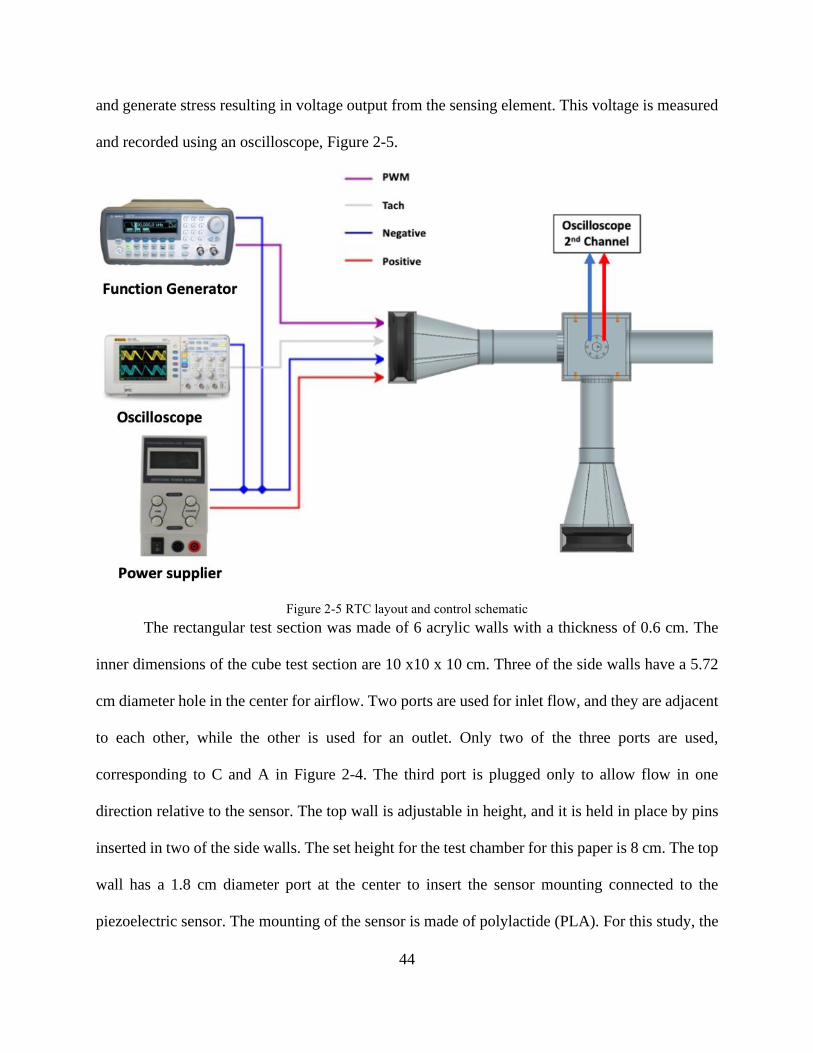
44
and generate stress resulting in voltage output from the sensing element. This voltage is measured
and recorded using an oscilloscope, Figure 2-5.
The rectangular test section was made of 6 acrylic walls with a thickness of 0.6 cm. The
inner dimensions of the cube test section are 10 x10 x 10 cm. Three of the side walls have a 5.72
cm diameter hole in the center for airflow. Two ports are used for inlet flow, and they are adjacent
to each other, while the other is used for an outlet. Only two of the three ports are used,
corresponding to C and A in Figure 2-4. The third port is plugged only to allow flow in one
direction relative to the sensor. The top wall is adjustable in height, and it is held in place by pins
inserted in two of the side walls. The set height for the test chamber for this paper is 8 cm. The top
wall has a 1.8 cm diameter port at the center to insert the sensor mounting connected to the
piezoelectric sensor. The mounting of the sensor is made of polylactide (PLA). For this study, the
Figure 2-5 RTC layout and control schematic

45
sensor is always placed perpendicular to the flow. A DC axial fan with a nominal voltage of 24V,
capable of running from 0-9500 RPM, provides the airflow. A power supply powers the fans. Each
fan is connected to the test chamber through an acrylic tube. A reduction adapter allows the flow
to go from the fan to the chamber inlets through the tubes. The generated signal is measured and
recorded by an oscilloscope.
2.2.2 Circular Test Section (CTS) Setup
Figure 2-6 presents the laboratory scale wind tunnel that is used for experimentation. The
wind tunnel has a 10 cm diameter test section. Similar to RTC, the working fluid is air. The sensing
element is mounted on a holder and maintained perpendicular to the airflow. Like the RTC, an
Figure 2-6 Experimental apparatus with circular test section (CTS)
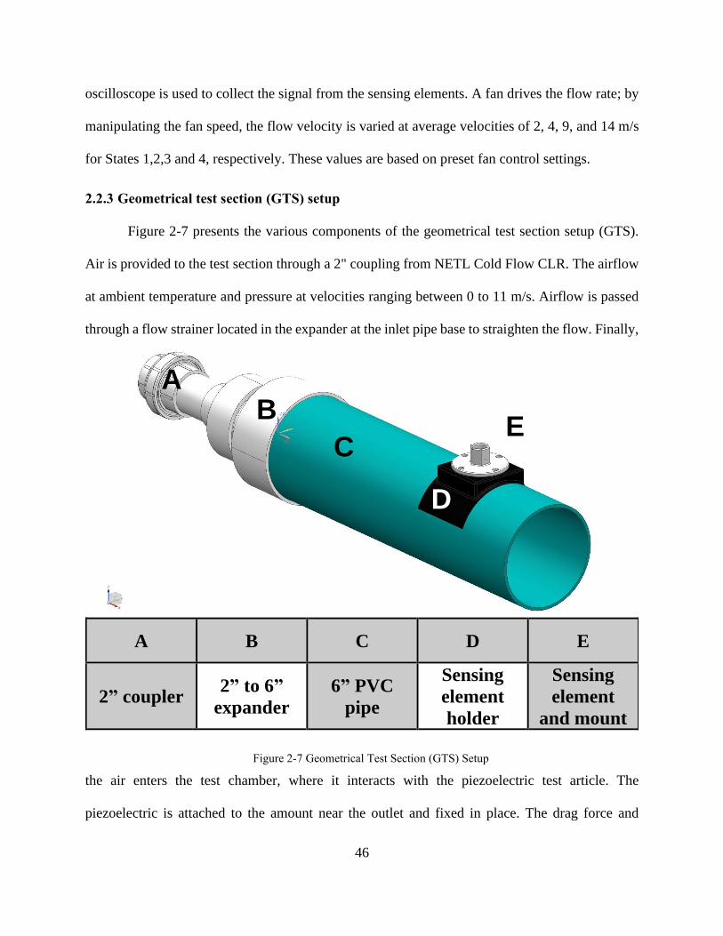
46
oscilloscope is used to collect the signal from the sensing elements. A fan drives the flow rate; by
manipulating the fan speed, the flow velocity is varied at average velocities of 2, 4, 9, and 14 m/s
for States 1,2,3 and 4, respectively. These values are based on preset fan control settings.
2.2.3 Geometrical test section (GTS) setup
Figure 2-7 presents the various components of the geometrical test section setup (GTS).
Air is provided to the test section through a 2" coupling from NETL Cold Flow CLR. The airflow
at ambient temperature and pressure at velocities ranging between 0 to 11 m/s. Airflow is passed
through a flow strainer located in the expander at the inlet pipe base to straighten the flow. Finally,
the air enters the test chamber, where it interacts with the piezoelectric test article. The
piezoelectric is attached to the amount near the outlet and fixed in place. The drag force and
Figure 2-7 Geometrical Test Section (GTS) Setup
E
D
C
B A
A B C D E
2” coupler 2” to 6”
expander
6” PVC
pipe
Sensing
element
holder
Sensing
element
and mount

47
pressure differences occurring in the test section cause the piezoelectric to vibrate and generate
stress resulting in voltage output from the sensing element. This voltage is measured and recorded
using a NI-DAQ, Figure 2-5.
The GTS was made of 6" PVC pipe as the testing chamber. The test chamber is connected
to the NETL air supply using a 2" coupler and two-step expander from 2"- 4" and 4"- 6". Inside
the test chamber, a 6" flow straightener to make the airflow more uniform before impact the test
article. The flow straightener was made of
PLA using a 3D printer at the University
of Texas at El Paso. The sensing element
holder and mount also 3d printed from
ABC using the NETL 3D printer. The
sensor is always placed perpendicular to
the flow.
As shown in Figure 2-8, the piezoelectric ceramic sensor was connected using an open-
circuit volt generator. A 560 𝑘Ω resiter was attached in parallel to the sensor; then, it is connected
to the data acquisition system, transferred, and saved the information to the computer.
Figure 2-8 GTS electrical connection diagram
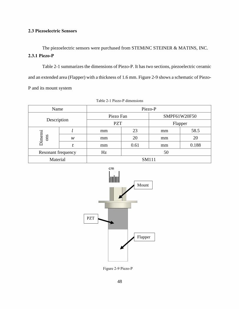
48
2.3 Piezoelectric Sensors
The piezoelectric sensors were purchased from STEMiNC STEINER & MATINS, INC.
2.3.1 Piezo-P
Table 2-1 summarizes the dimensions of Piezo-P. It has two sections, piezoelectric ceramic
and an extended area (Flapper) with a thickness of 1.6 mm. Figure 2-9 shows a schematic of Piezo-
P and its mount system
Table 2-1 Piezo-P dimensions
Name Piezo-P
Description Piezo Fan SMPF61W20F50
PZT Flapper
Dim
ensi
ons
𝑙 mm 23 mm 58.5
𝑤 mm 20 mm 20
𝑡 mm 0.61 mm 0.188
Resonant frequency Hz 50
Material SM111
Figure 2-9 Piezo-P
Mount
PZT
Flapper

49
2.3.2 Piezo-A
Table 2-2 summarizes the dimensions of Piezo-A
Table 2-2 Piezo-A dimensions
Name Piezo-A
Description SMPL14W9T15111
Dimensions
𝑙 Mm 14.4
𝑤 Mm 9.7
𝑡 Mm 1.5
Resonant frequency MHz 1.5
Material SM111
Figure 2-10 shows Piezo-A and its relative size to GTS setup
Figure 2-10 Piezo-A & its relative size to
setup
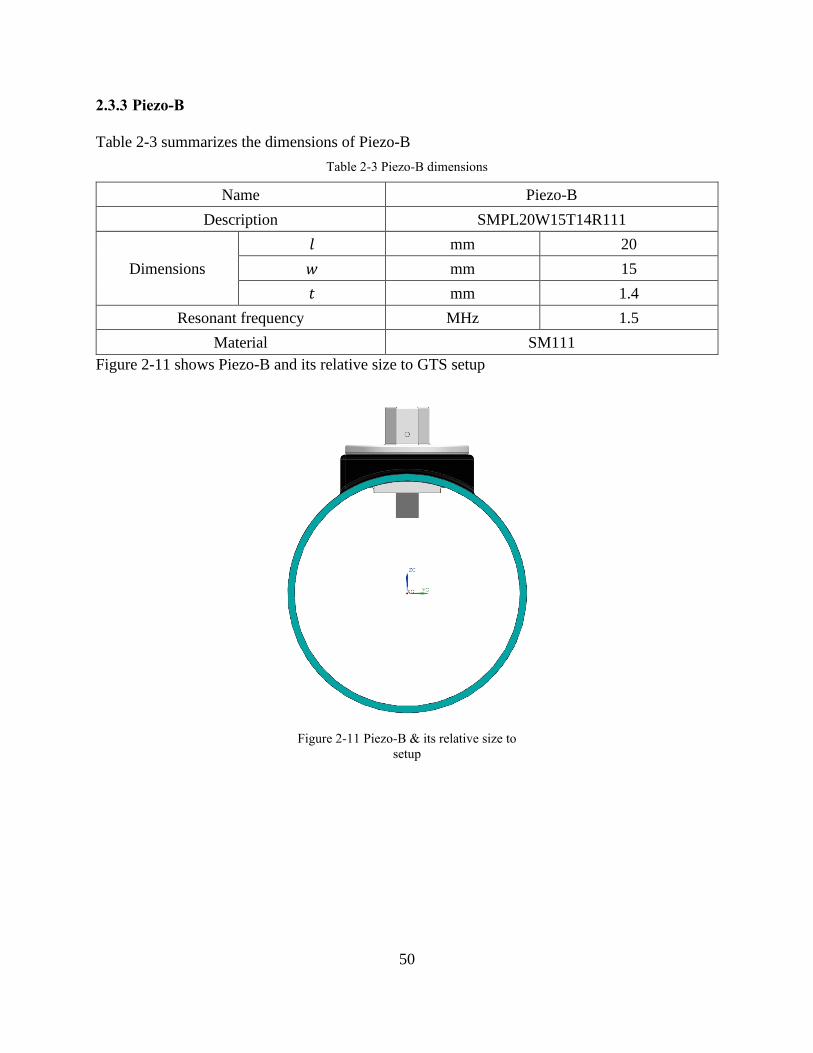
50
2.3.3 Piezo-B
Table 2-3 summarizes the dimensions of Piezo-B
Table 2-3 Piezo-B dimensions
Name Piezo-B
Description SMPL20W15T14R111
Dimensions
𝑙 mm 20
𝑤 mm 15
𝑡 mm 1.4
Resonant frequency MHz 1.5
Material SM111
Figure 2-11 shows Piezo-B and its relative size to GTS setup
Figure 2-11 Piezo-B & its relative size to
setup

51
2.3.4 Piezo-C
Table 2-4 summarizes the dimensions of Piezo-C
Table 2-4 Piezo-C dimensions
Name Piezo-C
Description SMPL20W15T1R111
Dimensions
𝑙 mm 20
𝑤 mm 15
𝑡 mm 1
Resonant frequency MHz 1.5
Material SM111
Figure 2-12 shows Piezo- and its relative size to GTS setup
Figure 2-12 Piezo-C & its relative size to
setup
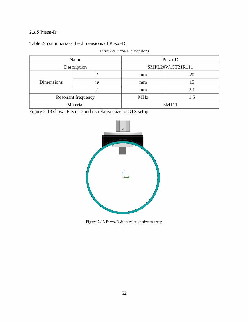
52
2.3.5 Piezo-D
Table 2-5 summarizes the dimensions of Piezo-D
Table 2-5 Piezo-D dimensions
Name Piezo-D
Description SMPL20W15T21R111
Dimensions
𝑙 mm 20
𝑤 mm 15
𝑡 mm 2.1
Resonant frequency MHz 1.5
Material SM111
Figure 2-13 shows Piezo-D and its relative size to GTS setup
Figure 2-13 Piezo-D & its relative size to setup
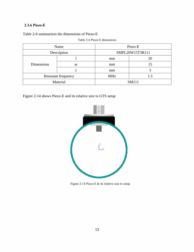
53
2.3.6 Piezo-E
Table 2-6 summarizes the dimensions of Piezo-E
Table 2-6 Piezo-E dimensions
Name Piezo-E
Description SMPL20W15T3R111
Dimensions
𝑙 mm 20
𝑤 mm 15
𝑡 mm 3
Resonant frequency MHz 1.5
Material SM111
Figure 2-14 shows Piezo-E and its relative size to GTS setup
Figure 2-14 Piezo-E & its relative size to setup
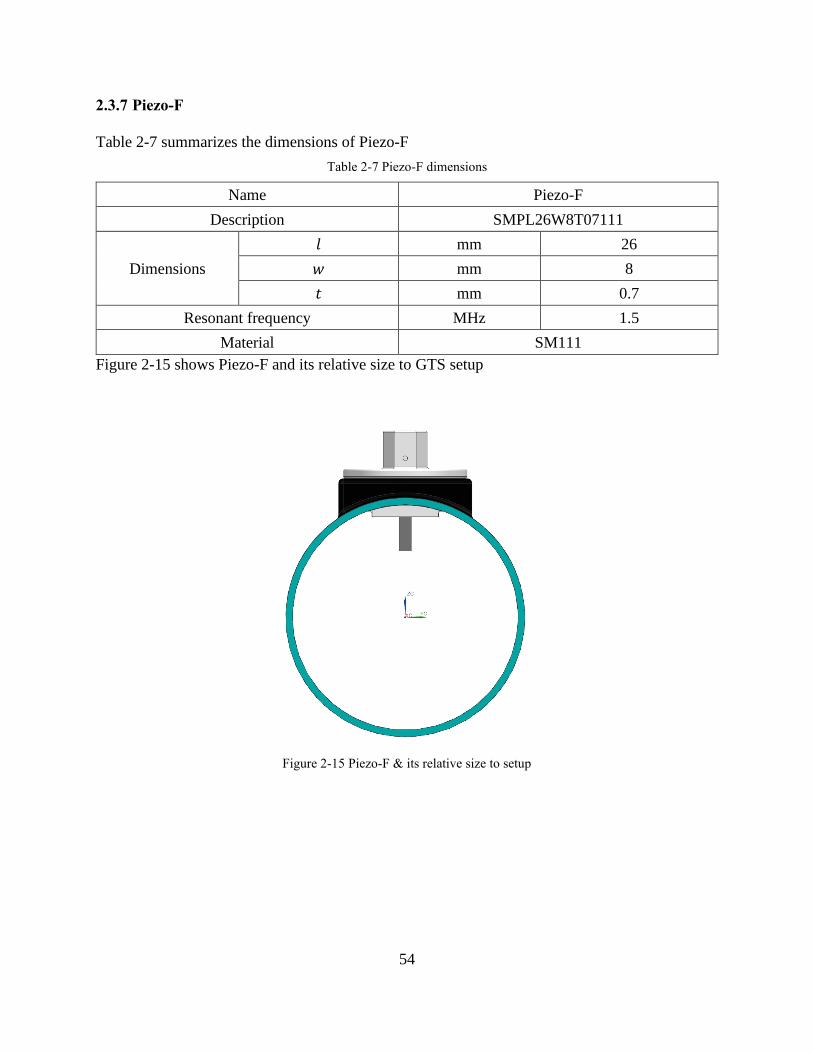
54
2.3.7 Piezo-F
Table 2-7 summarizes the dimensions of Piezo-F
Table 2-7 Piezo-F dimensions
Name Piezo-F
Description SMPL26W8T07111
Dimensions
𝑙 mm 26
𝑤 mm 8
𝑡 mm 0.7
Resonant frequency MHz 1.5
Material SM111
Figure 2-15 shows Piezo-F and its relative size to GTS setup
Figure 2-15 Piezo-F & its relative size to setup
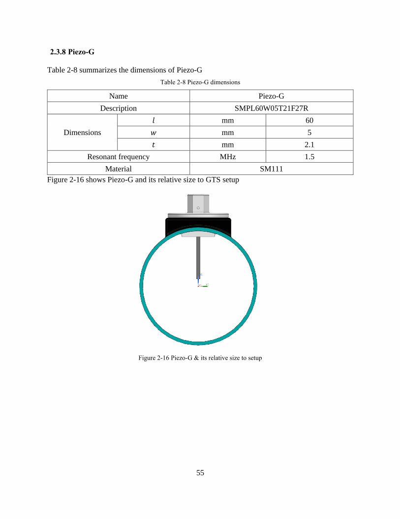
55
2.3.8 Piezo-G
Table 2-8 summarizes the dimensions of Piezo-G
Table 2-8 Piezo-G dimensions
Name Piezo-G
Description SMPL60W05T21F27R
Dimensions
𝑙 mm 60
𝑤 mm 5
𝑡 mm 2.1
Resonant frequency MHz 1.5
Material SM111
Figure 2-16 shows Piezo-G and its relative size to GTS setup
Figure 2-16 Piezo-G & its relative size to setup
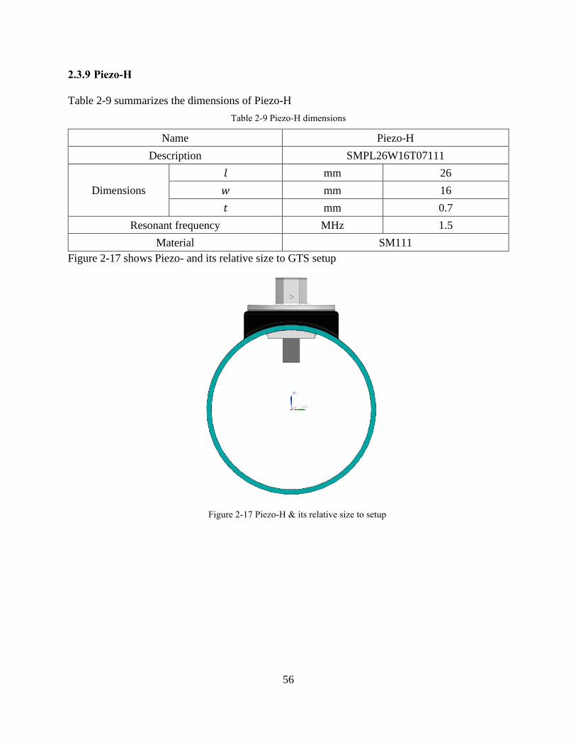
56
2.3.9 Piezo-H
Table 2-9 summarizes the dimensions of Piezo-H
Table 2-9 Piezo-H dimensions
Name Piezo-H
Description SMPL26W16T07111
Dimensions
𝑙 mm 26
𝑤 mm 16
𝑡 mm 0.7
Resonant frequency MHz 1.5
Material SM111
Figure 2-17 shows Piezo- and its relative size to GTS setup
Figure 2-17 Piezo-H & its relative size to setup
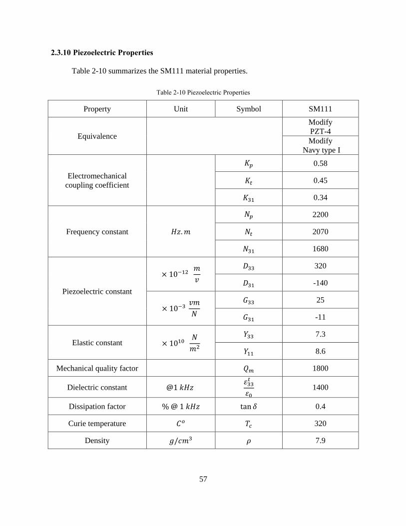
57
2.3.10 Piezoelectric Properties
Table 2-10 summarizes the SM111 material properties.
Table 2-10 Piezoelectric Properties
Property Unit Symbol SM111
Equivalence
Modify
PZT-4
Modify
Navy type I
Electromechanical
coupling coefficient
𝐾𝑝 0.58
𝐾𝑡 0.45
𝐾31 0.34
Frequency constant 𝐻𝑧.𝑚
𝑁𝑝 2200
𝑁𝑡 2070
𝑁31 1680
Piezoelectric constant
× 10−12 𝑚
𝑣
𝐷33 320
𝐷31 -140
× 10−3 𝑣𝑚
𝑁
𝐺33 25
𝐺31 -11
Elastic constant × 1010 𝑁
𝑚2
𝑌33 7.3
𝑌11 8.6
Mechanical quality factor 𝑄𝑚 1800
Dielectric constant @1 𝑘𝐻𝑧 휀33𝑡
휀0 1400
Dissipation factor % @ 1 𝑘𝐻𝑧 tan 𝛿 0.4
Curie temperature 𝐶𝑜 𝑇𝑐 320
Density 𝑔/𝑐𝑚3 𝜌 7.9

58
2.4 List of instrumentation
Below is a list of the instruments used for this project.
2.4.1 DC Axial Compact fan
An axial fan is a fan that causes fluid to flow across it in an axial direction, parallel to the
shaft, which the blades rotate about it. The fan is designed to produce a pressure difference to cause
a flow through the fan.
A 4-WIRE fan has power, ground, and tach signal, which provides a signal with a
frequency proportional to speed, a PWM input used to control the fan's speed. As A Substitute for
switching the power to the entire fan ON and OFF, only the drive coils' power is switched, making
the tach information available continuously. In brief, PWM uses the relative width of pulses in a
line up of on-off pulses to adjust the amount of power applied to the motor. Another advantage of
4-wire fans is that the fan speed can be controlled at speeds as low as 10% of the fan's full speed.
A 4114 N/2H7P DC Axial compact fan is used as it provides all characteristics for the experimental
Figure 2-18 6" DC Axial Compact Fan

59
setup. It is a clockwise rotor fan whose speed control range varies from 500 rpm-1 up to 950 rpm-
1. At 0% PWM, maximum speed if control cable (PWM) is interrupted.
2.4.2 Power Supply
The CSI3005SM is a compact benchtop linear power supply. For appliances that
require a decent amount of clean power, this unit can deliver up to 30 volts and 5 amps.
The user can preset the current and voltage output via two sets of multi-turn dials that
offer rough and slight adjustments for precise settings. The power supply provides
constant power to the DC Axial fan of 24V.
Figure 2-19 Power Supply

60
2.4.3 Function Generator
A function generator is an essential piece of electronic gear or software used to generate
different electrical waveforms over a wide-ranging of frequencies. Some of the most frequent
waveforms produced by the function generator are the sine wave, square wave, triangular wave,
and sawtooth shapes.
The Agilent Technologies 33210A used creates stable, accurate low distortion sine waves
and square waves with the rapid rise and fall times of 10 MHz and linear ramp waves up to 100
kHz. The square wave is a specific case of a pulse wave that allows arbitrary duration at minimum
and maximum. The high-level period to the total period of a pulse wave is known as the duty cycle.
The fan's duty cycle can be controlled using the apparatus, ranging from 20 to 100 %, meaning an
increment or decrease on the fan's RPM's.
Figure 2-20 Function Generator

61
2.4.4 Hotwire Anemometer
The anemometer used in this study provides multiple features that make it suitable to use
in such applications as environmental testing, balancing of fans/motors/blowers, air conveyors,
clean rooms, and flow hoods. The apparatus measures velocity and air temperature and has an
input socket that accepts a Type J or K thermocouple that can be used as a highly accurate
thermometer. The integrated hot wire and standard thermistors provide fast and accurate readings
even at low velocities.TES 1341 Hot-Wire Anemometer, the Portable Air Velocity Meter is a
lightweight instrument that can be used anywhere to measure air velocity. The Velocity Probe
range between 0 to 30 m/s (0 to 6000 ft/min) with -Resolution of 0.01 m/s (1 ft/min) and Accuracy:
±3% of reading ±1%FS
Figure 2-22 HWA2005DL Hot
Wire Anemometer with Real-Time
Data Logger Figure 2-21 TES 1341 Hot-Wire anemometer

62
2.4.5 Oscilloscope
An oscilloscope is used to show and analyze the waveform of electronic signals. Essentially,
the device draws a graph of the instantaneous signal voltage as a function of time. The horizontal
sweep is evaluated in seconds per division in any oscilloscope, and the vertical deflection is
measured in volts per division. It has multiple inputs, called channels, and each one of these acts
independently.
A RIGOL DS1102E Oscilloscope has a sampling rate of 1GSa/s maximum real-time
sample rate and 25GSa/s maximum equivalent sample rate, with a Bandwidth of 100MHz per
channel. It has a maximum 16k- point regular record length and one million points on maximum
record length.
Table 2-11 Oscilloscope configuration
Channel Mode Sample rate Memory Depth
(average)
Memory Depth
(a long record)
Single channel 1GSa/s 16kpts N.A.
Single channel 500MSa/s or lower 16kpts 1Mpts
Dual channel 500MSa/s or lower 8kpts N.A.
Dual channel 250MSa/s or lower 8kpts 512kpts
The oscilloscope can be adjusted to observe repetitive signals as a continuous shape on the
screen. Using real-time sampling configuration, the oscilloscope samples the waveform often
enough to capture the waveform's complete image with each acquisition. The oscilloscopes can
Figure 2-23 Oscilloscope

63
capture complex signals in great detail over extended periods to utilize the extended memory,
which allows an observer to examine high-frequency effects within the captured waveform.
Typically, when multiple channels are in use, the sample rate is split up among the channels.
So, looking at long periods with a high resolution between points, deep memory will be
needed. A sample rate must be required to provide enough detail to see any unexpected glitches or
anomalies. To utilizing the extended memory, RIGOL scopes can capture complex signals in great
detail over extended periods. This allows an observer to examine high-frequency effects within
the captured waveform. For the data analysis, data is imported from the Oscilloscope and then
transferred to MS Excel; it will then be used to analyze the measurement data obtained from the
experiment.

64
2.4.6 NI-9215 with BNC DAQ
The NI 9215 is an analog input module for use with NI CompactDAQ and CompactRIO
systems. The NI 9215 includes four simultaneously sampled analog input channels and successive
approximation register (SAR) 16-bit analog-to-digital converters (ADCs) with a 100 kS/s/ch
sample rate.
The NI 9215 contains NIST-traceable calibration, a channel-to-earth ground double
isolation barrier for safety and noise immunity, and a high common-mode voltage range.
Figure 2-24 NI-9215 with BNC DAQ
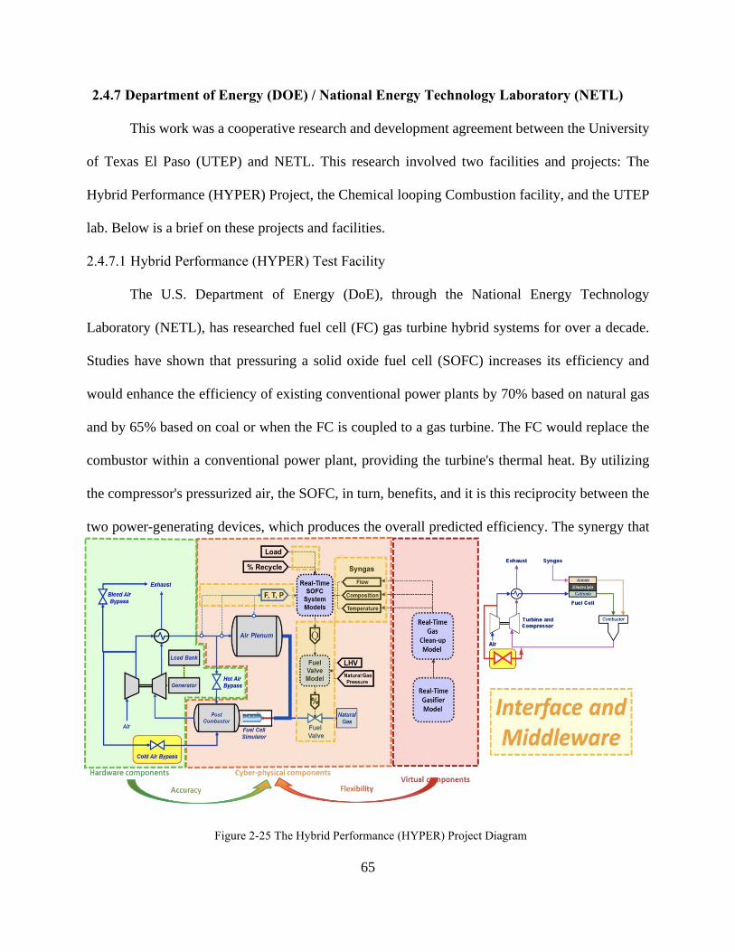
65
2.4.7 Department of Energy (DOE) / National Energy Technology Laboratory (NETL)
This work was a cooperative research and development agreement between the University
of Texas El Paso (UTEP) and NETL. This research involved two facilities and projects: The
Hybrid Performance (HYPER) Project, the Chemical looping Combustion facility, and the UTEP
lab. Below is a brief on these projects and facilities.
2.4.7.1 Hybrid Performance (HYPER) Test Facility
The U.S. Department of Energy (DoE), through the National Energy Technology
Laboratory (NETL), has researched fuel cell (FC) gas turbine hybrid systems for over a decade.
Studies have shown that pressuring a solid oxide fuel cell (SOFC) increases its efficiency and
would enhance the efficiency of existing conventional power plants by 70% based on natural gas
and by 65% based on coal or when the FC is coupled to a gas turbine. The FC would replace the
combustor within a conventional power plant, providing the turbine's thermal heat. By utilizing
the compressor's pressurized air, the SOFC, in turn, benefits, and it is this reciprocity between the
two power-generating devices, which produces the overall predicted efficiency. The synergy that
Figure 2-25 The Hybrid Performance (HYPER) Project Diagram

66
results in this concept holds the promise of a reduced emissions system with the potential to include
renewable energy sources[65]. The experiments were carried out using a cyber-physical simulation
approach. In this method, the hardware components of the HyPer facility were coupled with a real-
time numerical model of the Solid Oxide Fuel Cell (SOFC), which led to the heat source of the
system. The fuel cell emulator's hardware components included a natural gas combustor to
simulate the fuel cell's heat and two vessels to mimic the fuel cell system's volumes. They were
physically coupled to a recuperated gas turbine. A diagram representation of the plant is presented
in Figure 2-25. The model also contains a dynamic module of a biomass gasifier, not included in
this work. The turbine exhaust preheated the compressed air into the two counter-flow heat
exchangers before supplying the cathode and air manifold volumes emulator. The pressure
dynamics of the fuel cell have been replicated. After the volume, a natural gas combustor produced
the heat calculated in the fuel cell model. A second vessel was positioned after the combustor to
simulate the post-combustor volume in the fuel cell system. Three bypass valves were used for
regulating purposes:1) Bleed air valve, which blew compressed air into the atmosphere, 2) Cold
air bypass, which diverted air from the compressor outlet to the post-combustor volume, and 3)
Hot air bypass, which was positioned at the heat exchangers outlet and bypassed the fuel cell
emulator. A cold air valve was observed to impact cathode airflow, turbine inlet temperature,
turbine speed, system pressures, and surge margin. It was considered an essential actuator because
it is advantageous in varying fuel cell temperature distribution. Hence, its complete
characterization was considered fundamental for system control. [66]
The plenum of air for this system is significantly larger, two orders of magnitude, than the
typical compressor volume for this type of cycle. The large volume results in a complicated
dynamic response of the system. For example, change in turbine operating conditions caused by

67
load variation, fuel, or heat absorption in the SOFC result in different inlet airflow and pressure
ratios in the compressor because of the system's large volume. This method results in complicated
compressor dynamics and tends to result in challenging behaviors to predict in advance, once such
behavior is compressor surge. Compressor surge can be destructive for both the turbomachinery
and the SOFC. If the compressor dynamics could be controlled at a rate that is faster than existing
hardware allows, compressor surge may be detected and avoided before causing damage, as
mentioned before. [67]
Love et al. and Lin et al. have investigated the use of piezoelectric/pyroelectric sensors for
various power generation monitoring applications. The proposed project recently developed a
sensor capable of measuring instantaneous temperature and pressure measurements with a wafer
of Lithium Niobate (LiNbO3)[42], [68]. The wafer could be placed on the surface of the
measurement point of interest. Once in place, the material generates a current when exposed to a
temperature or pressure change with time. The current generated by the sensor can be calibrated
to represent changes in temperature or pressure, depending on the application. Recent work by
Love et al. and Lin et al. have demonstrated the sensor's ability to be used in a wired or wireless
design to measure temperature. Pressure measurements have also been demonstrated using a lower
temperature material, Lead-Ziroconate Titanate (PZT); however, it could easily be demonstrated
using the Lithium Niobate sensor instead. Lithium Niobate is preferable for most applications
involving a harsh environment because of the higher Curie temperature of 1210oC and tunable
frequency response time up to the 1 MHz range. [43], [69] Besides, they have successfully
demonstrated the feasibility of printing piezoelectric ceramics with designed geometry for specific
temperature and pressure sensing applications.

68
The HYPER facility's operation may be improved, and compressor stall is mitigated during
periods of transient operation if rapidly responding measurement sensors developed by this study
could be coupled with existing control strategies developed by NETL. One proposed method may
be the detection parameters such as mass flow rate, temperature, or pressure downstream of the
compressor exit at frequencies of 200Hz.
In this system, the air is extracted from the compressor and fed to the cathode side of SOFC.
The volume of a hybrid involves two orders of magnitude more than the compressor plenum
volume of a simple cycle, which results in a degradation of compressor surge margin and complex
compressor dynamics. When turbine rotational speed is reduced during transients, compressor inlet
airflow and pressure ratio decrease at different rates due to large volume. In this case, the
compressor map's operating point can follow a path toward the stall line. Drastic changes in turbine
load or fuel or sudden heat absorption in the fuel cell stack, for example, can thus lead the
compressor operation close to stall and surge conditions if not mitigated.[67]
2.4.7.2 Chemical looping Combustion facility
Chemical looping (CL) is a process to indirectly oxidize fuels with air, transforming the
chemical energy in fuels to thermal energy. On the other hand, to direct oxidation with air, carbon
dioxide and nitrogen are in different exhaust streams. This technology facilitates the sequestration
of CO2 without a separate gas separation system before (e.g., oxy-fuel combustion) or after the
combustor. The system only requires a condenser to eliminate the water. As shown in Figure 2-26,
the left is a diagram of the CL system based on two fluidized bed reactors. Solid particles have
circulated the loop, which oxidizes in the air reactor and reduces in the fuel reactor. Regular carrier
materials include metals such as copper, iron, or nickel. The air reactor's reaction is usually

69
exothermic, while the reaction in the fuel reactor can be somewhat endothermic or exothermic
depending on the fuel gas composition and the carrier used. Many proposed designs use the
circulating solids' thermal energy to provide the necessary heat to maintain the fuel reactor's
temperature for endothermic systems. From the standpoint of and modeling simulation, NETL has
three systems onsite to validate chemical looping models. Several smaller systems (TGA and fixed
bed) are used for the calibration of reaction models.
In Figure 2-27, The leftmost figure shows the "single fluid bed" reactor. The reactor has a
2.5-inch inner diameter and is insulated and heated to maintain a specified operating temperature.
This apparatus investigates interactions between flow dynamics and reactivity on a smaller, more
controlled size than the CLR.
Figure 2-26 Chemical Looping Diagram

70
The center figure illustrates the chemical looping reactor (CLR). The structure is several
meters high and has a design capacity of 50kW thermal power. The air reactor is 6 inches in
diameter, and the fuel reactor is 8 inches in diameter.
The rightmost figure shows the cold flow (CLR). It has approximately the same geometry
as the CLR. This system is used to guide the full system's operation and general exploration of
circulating chemical looping systems' dynamics. The system can run in both batches of circulation
modes. The NETL Cold Flow CLR facility had an air supply with a volumetric flow rate of up to
24000 SCFH and ambient pressure. [70]
Figure 2-27 NETL Chemical looping experimental systems

71
2.5 Test Matrix
As mentioned in the Theory section, the project has three phases. Below are the details of
the experiments used to fulfill the three phases of the project.
2.5.1 Phase-I: Piezoelectric as a Flow Rate Sensor
The velocity inside the RTS and CTS will be measured using the hotwire anemometer. The
anemometer will be at the same location as the piezoelectric sensor. The velocity profile for both
setups will be measured at different vertical points. The experiment will be repeated five times.
The velocity will be varied according to the state mentioned in the experiment setup, and each
state will be repeated five times. Then, the statistical study will be performed on the data.
The flow rate will be calculated from the velocity study, as shown in equation 2.9, based
on each setup's cross-section duct area.
𝑉 = 𝐴𝑐 𝑣 2.9
Where:
𝑉 : the volumetric flow rate [m3/s]
𝐴𝑐: the cross-section area [m2]
𝑣 : the average velocity [m/s]
The main force acting on the piezoelectric is assumed to be a drag. The drag force will be
estimated from the average velocity acting on the piezoelectric surface, as shown in equation 2.10.
𝐹𝐷 =
1
2 𝐶𝐷 𝜌 𝐴 𝑣
2 2.10

72
The Piezo-P will be inserted in RTS and CTS, the flow rate will be varied, and the sensor's
voltage output will be collected. Table 2-12 shows the test plan, and the four different states
correspond to different preset values on each experimental setup.
Table 2-12 Velocity variation for CTS and RTS
Velocity (𝑚/𝑠)
CTS Setup
State 1 State 2 State 3 State 4
RTS Setup
The velocity profile inside the CTS and RTS setups will be measured at the test article's
location with a cross-section height variation. The same method was used before for statistical
analysis. After that, in one of the previous states, where the average velocity was close, the voltage
output will be collected. This procedure will validate Phase 2 if the velocity profile affects the
voltage output. The case plan is shown in Table 2-13
Table 2-13 Duct Shape variation at the same velocity
Piezo-P
CTS State 2
RTS State 2

73
2.5.2 Phase-II: Geometrical effect and Empirical Equation
Equation 2.7 can be written as
𝐿𝑜𝑔10(𝑉) = 𝐿𝑜𝑔10(𝑎) + 𝑏 𝐿𝑜𝑔10 (
𝑙
𝑤) + 𝑐 𝐿𝑜𝑔10 (
𝐴
𝑡) + 𝑑 𝐿𝑜𝑔10(𝑣)
2.11
From crossing equations 2.8 and 2.11, the coefficient could be written as
𝛽0 = 𝐿𝑜𝑔10(𝑎), 𝛽1 = 𝑏, 𝛽2 = 𝑐, 𝛽3 = 𝑑 2.12
Equations 2.11and 2.12 show that the voltage output is the primary variable and correlation
that needs to be defined from experimental tests summaries of the test specimens to be tested in
this phase.
Table 2-14 Piezo cases dimension summary
Name
Dimensions Area
𝑤 𝑙 𝑡
mm mm mm mm2
A 14.4 9.7 1.5 140
B 20 15 1.4 300
C 20 15 1 300
D 20 15 2.1 300
E 20 15 3 300
F 26 8 0.7 208
G 60 5 2.1 300
H 26 16 0.7 416
The piezo specimen will be inserted in GTS, and the flow will be changed according to the
state mentioned before. The change in flow will be shown in Figure 2-28
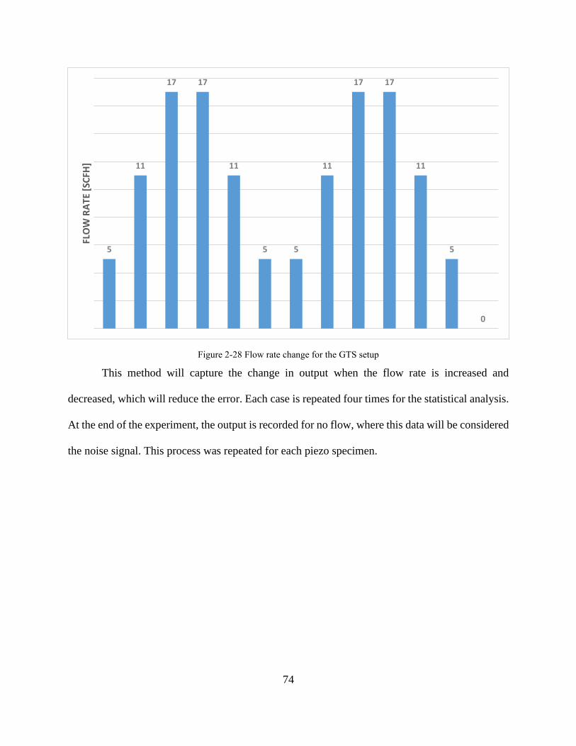
74
This method will capture the change in output when the flow rate is increased and
decreased, which will reduce the error. Each case is repeated four times for the statistical analysis.
At the end of the experiment, the output is recorded for no flow, where this data will be considered
the noise signal. This process was repeated for each piezo specimen.
5
11
17 17
11
5 5
11
17 17
11
5
0
FLO
W R
AT
E [S
CFH
]
Figure 2-28 Flow rate change for the GTS setup

75
Chapter 3: Results and discussion
In this chapter, the data from phase-I is presented and displayed
3.1 Results and discussion for phase-I
3.1.1 Velocity Profile Results
The average velocity acting on the piezoelectric surface was calculated by measuring the
velocity profile inside the CTS and RTC test section with a hotwire anemometer. It was were
measured at the same location as the position of the piezoelectric sensor. The velocity profiles
within the test sections were measured at preset settings of States 1 to 4. The velocities associated
with these states are presented in Table 3-1. The four different states correspond to different preset
values on each experimental setup.
Table 3-1 Velocities tested in the circular and rectangular test section setups
CTS Average Velocity
(m/s)
RTS Average Velocity
(m/s)
State 1 1.9 2.83
State 2 4.3 4.41
State 3 9.0 9.06
State 4 14.5 `
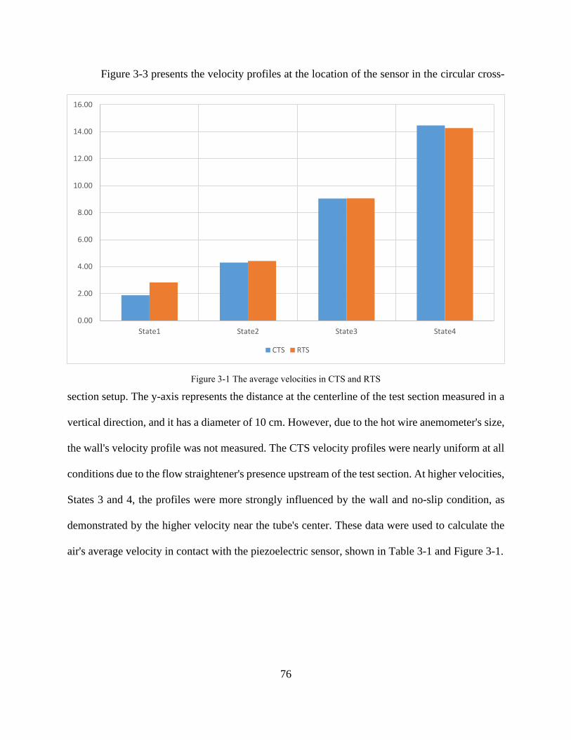
76
Figure 3-3 presents the velocity profiles at the location of the sensor in the circular cross-
section setup. The y-axis represents the distance at the centerline of the test section measured in a
vertical direction, and it has a diameter of 10 cm. However, due to the hot wire anemometer's size,
the wall's velocity profile was not measured. The CTS velocity profiles were nearly uniform at all
conditions due to the flow straightener's presence upstream of the test section. At higher velocities,
States 3 and 4, the profiles were more strongly influenced by the wall and no-slip condition, as
demonstrated by the higher velocity near the tube's center. These data were used to calculate the
air's average velocity in contact with the piezoelectric sensor, shown in Table 3-1 and Figure 3-1.
0.00
2.00
4.00
6.00
8.00
10.00
12.00
14.00
16.00
State1 State2 State3 State4
CTS RTS
Figure 3-1 The average velocities in CTS and RTS
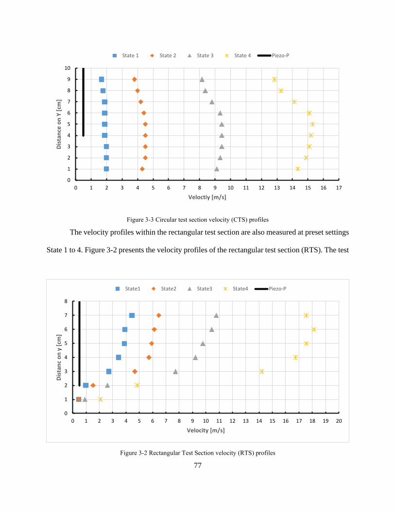
77
The velocity profiles within the rectangular test section are also measured at preset settings
State 1 to 4. Figure 3-2 presents the velocity profiles of the rectangular test section (RTS). The test
0
1
2
3
4
5
6
7
8
9
10
0 1 2 3 4 5 6 7 8 9 10 11 12 13 14 15 16 17
Dis
tan
ce o
n Y
[cm
]
Veloctiy [m/s]
State 1 State 2 State 3 State 4 Piezo-P
Figure 3-3 Circular test section velocity (CTS) profiles
0
1
2
3
4
5
6
7
8
0 1 2 3 4 5 6 7 8 9 10 11 12 13 14 15 16 17 18 19 20
Dis
tan
c o
n y
[cm
]
Velocity [m/s]
State1 State2 State3 State4 Piezo-P
Figure 3-2 Rectangular Test Section velocity (RTS) profiles

78
section has a height of 8 cm. Near wall velocities were not recorded due to the hot wire
anemometer's size. For these velocity profiles, low velocity is measured near the bottom and top
Figure 3-3 and Figure 3-2, the velocities profiles are different for each setup. The main
differences between the two setups are the velocity profile and the duct's height, which impact the
region where the stream interacts with the Piezo-P.
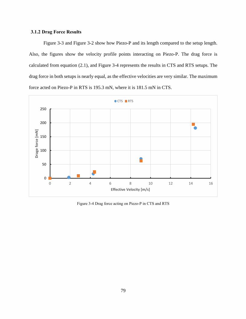
79
3.1.2 Drag Force Results
Figure 3-3 and Figure 3-2 show how Piezo-P and its length compared to the setup length.
Also, the figures show the velocity profile points interacting on Piezo-P. The drag force is
calculated from equation (2.1), and Figure 3-4 represents the results in CTS and RTS setups. The
drag force in both setups is nearly equal, as the effective velocities are very similar. The maximum
force acted on Piezo-P in RTS is 195.3 mN, where it is 181.5 mN in CTS.
0
50
100
150
200
250
0 2 4 6 8 10 12 14 16
Dra
ge f
orc
e [
mN
]
Effective Velocity [m/s]
CTS RTS
Figure 3-4 Drag force acting on Piezo-P in CTS and RTS
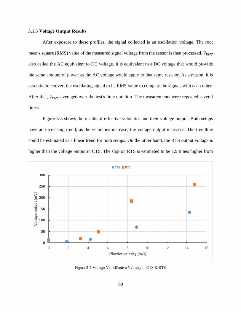
80
3.1.3 Voltage Output Results
After exposure to these profiles, the signal collected is an oscillation voltage. The root
means square (RMS) value of the measured signal voltage from the sensor is then processed. 𝑉𝑅𝑀𝑆
also called the AC equivalent to DC voltage. It is equivalent to a DC voltage that would provide
the same amount of power as the AC voltage would apply to that same resistor. As a reason, it is
essential to convert the oscillating signal to its RMS value to compare the signals with each other.
After that, 𝑉𝑅𝑀𝑆 averaged over the test's time duration. The measurements were repeated several
times.
Figure 3-5 shows the results of effective velocities and their voltage output. Both setups
have an increasing trend; as the velocities increase, the voltage output increases. The trendline
could be estimated as a linear trend for both setups. On the other hand, the RTS output voltage is
higher than the voltage output in CTS. The slop on RTS is estimated to be 1.9 times higher from
0
50
100
150
200
250
300
0 2 4 6 8 10 12 14 16
Vo
ltag
e o
utp
ut
[mV
]
Effective velocity [m/s]
CTS RTS
Figure 3-5 Voltage Vs. Effective Velocity in CTS & RTS
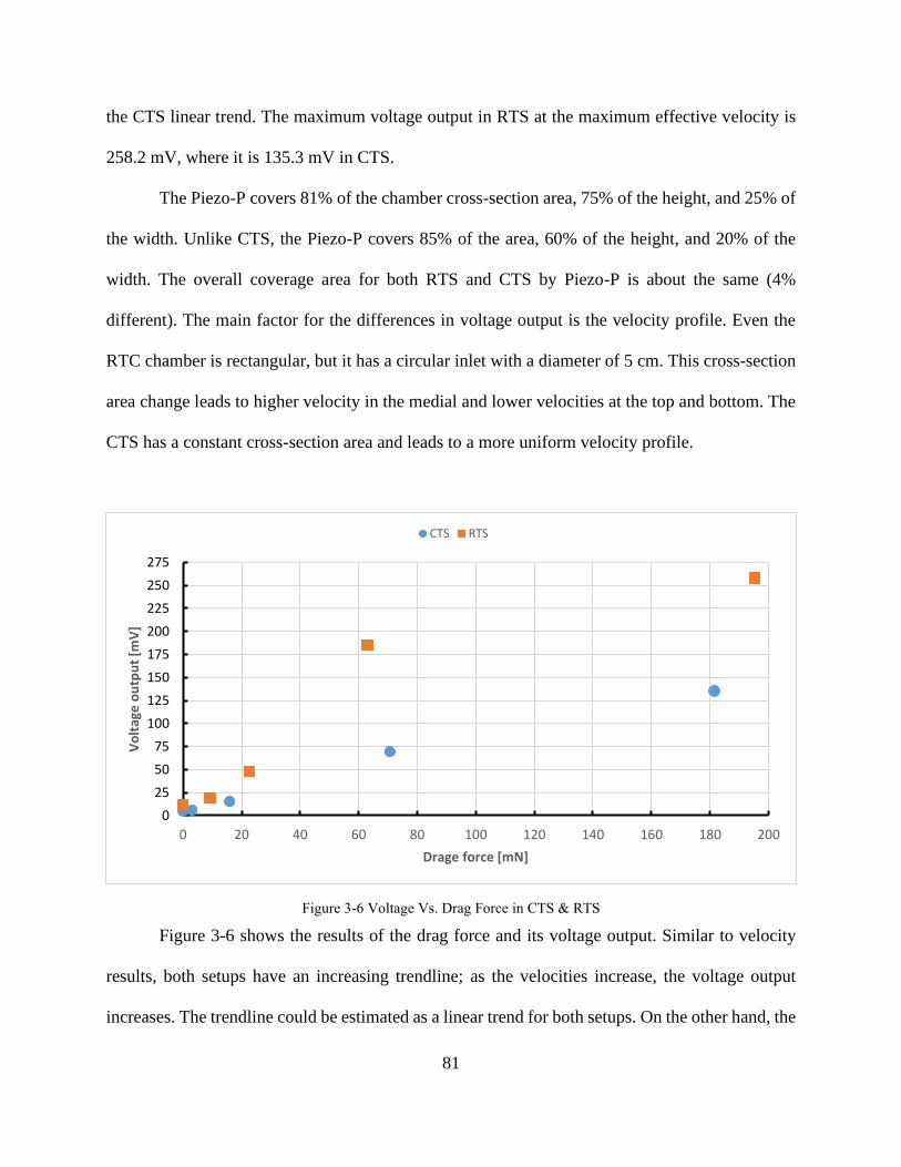
81
the CTS linear trend. The maximum voltage output in RTS at the maximum effective velocity is
258.2 mV, where it is 135.3 mV in CTS.
The Piezo-P covers 81% of the chamber cross-section area, 75% of the height, and 25% of
the width. Unlike CTS, the Piezo-P covers 85% of the area, 60% of the height, and 20% of the
width. The overall coverage area for both RTS and CTS by Piezo-P is about the same (4%
different). The main factor for the differences in voltage output is the velocity profile. Even the
RTC chamber is rectangular, but it has a circular inlet with a diameter of 5 cm. This cross-section
area change leads to higher velocity in the medial and lower velocities at the top and bottom. The
CTS has a constant cross-section area and leads to a more uniform velocity profile.
Figure 3-6 shows the results of the drag force and its voltage output. Similar to velocity
results, both setups have an increasing trendline; as the velocities increase, the voltage output
increases. The trendline could be estimated as a linear trend for both setups. On the other hand, the
0
25
50
75
100
125
150
175
200
225
250
275
0 20 40 60 80 100 120 140 160 180 200
Vo
ltag
e o
utp
ut
[mV
]
Drage force [mN]
CTS RTS
Figure 3-6 Voltage Vs. Drag Force in CTS & RTS

82
RTS output voltage is higher than the voltage output in CTS. Like the velocity plot, the slop on
RTS is estimated to be 1.9 times higher from the CTS linear trend and trend. The maximum voltage
output in RTS at the maximum effective velocity is 258.2 mV, where it is 135.3 mV in CTS.
Even the relationship between drag force and velocity is quadratic, the relationship between
drag force and velocities kept a linear relationship with voltage output with the same slope. The
linear relationship is essential for the sensor output as it makes signal processing and results more
consistent.

83
3.1.4 Signal to Noise Ratio results
SNR's importance is showing the signal's quality; the higher the ratio, the better signal.
Defining noise is a significant concern for all signal outputs, becoming overly complicated and
changing this study's focus. As a reason, the noise for this study is defined as a signal collected
when airflow is at 0for 1 minute. This noise is estimated to have most of the external and internal
noise. Figure 3-7 shows how the signal to noise ratio (SNR) for each state voltage output. The
SNR is calculated from equation (1.28). It is very close in results between CTS and RTS, which
means the change in velocity profile or the duct shape has no effect on SNR and is mainly a factor
of the piezoelectric material and its shape and geometry.
0.0
5.0
10.0
15.0
20.0
25.0
30.0
35.0
State 0 State 1 State 2 State 3 State 4
Sign
al t
o N
ois
e R
atio
(SN
R)
[dB
]
CTS RTS
Figure 3-7 Signal to Noise Ratio in Piezo-P

84
3.2 Results and discussion for phase-II
After exposure to each piezos for Cases from 0 to 3, the data was collected with NI-9215
DAQ and processed through NI DIAdem. The experiments were conducted in two cycles. The
cycle is case 1, case 2, case 3, case 3, case2, case 1, which correspond to the following velocities.
Units Case 0 Case 1 Case 2 Case 3
Velocity m/s 0.0 2.24 4.85 7.56
This cycle was repeated for the statistical study. After that, case 0 is conducted to collect
references and noise. The sample rate used for data acquisition is 4.25 𝜇𝑠, and the time recorded
was about five minutes for each case for each piezo. The total cases evaluated were 114 cases; the
accepted cases are 102 cases with an average duration for each piezo of 85 min. To be able to
collect data, a 560 𝑘Ω resister is connected at the two electrodes and the DAQ.
The detected frequency was determined by applying Forward Fourier Transfer (FFT) on
the signal. After the oscillation, data was transferred into the root mean square value (RMS) to
show the effective voltage. As the testing time contained increasing in the flow (or decreasing) to
go from one case to another, the data included a transfer and steady states. As a reason, dividing
the signal was required to split the two states where the steady-state was selected to show the
geometrical effect on steady operating conditions. (The transient state could be studied later to
determine the response time as other transient factors, but it was out of the scope of this project.)
Due to the large amount of data collected, an automated algorithm needed to process this
data and decided at which time (or point) the data considered changed from transient to steady-
state. The point was chosen based on the flow rate data as this data was more reliable, consistent,
and accurate. (the NETL officials provided the data). The separating point was determined based
on the signal's histogram, where the most repeated value was considered steady-state value. After

85
that, the equivalent time for this value was looked up and recorded. The time value was then looked
up in the RMS voltage signal and the data divided at this point. The data after the selected point is
considered steady-state, and before the point is transient. The steady-state values are then averaged
over the duration and categorized bases on Case 0, Case 1, Case 2, and Case 3. Then each matching
case was averaged, and statistical analysis was conducted on them. The following shows the final
results.
3.2.1 Velocity results
The average velocity acting on the piezoelectric surface was calculated by measuring the
CLR mass flow controller's volumetric flow rate pass in the GTS test section. Three flow rates
were chosen to cover the range of operation. Low, medium, and high flow rates at 5000, 11000,
and 17000 SCFH, respectively, are equivalent to 3.97E-2, 8.60E-2, and 1.34E-1 m3/s. Also, they
are called Case 1, Case 2, and Case 3, respectively. In addition to these cases, a reference case was
conducted at no flow condition to count for the noises. Table 3-2 and Figure 3-8 show the resulting
velocities for each case. The relationship between the velocities and the flow rate is linear. The
mean velocities for each case are 0, 2.24, 4.85, and 7.56 m/s, respectively. The collected data has
a small error in general, and case 2 has the highest error of 0.26 m/s variation of the mean. These
velocities will be used for all the specimens calculation in this phase.
Table 3-2 Velocity Vs. Flow rate results
Units Case 0 Case 1 Case 2 Case 3
Flow rate m3/s 0.0 3.97E-2 8.60E-2 1.34E-1
Velocity m/s 0.0 2.24 4.85 7.56
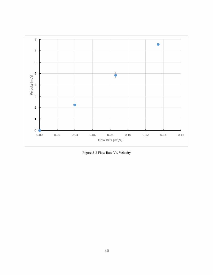
86
0
1
2
3
4
5
6
7
8
0.00 0.02 0.04 0.06 0.08 0.10 0.12 0.14 0.16
Ve
loci
ty [
m/s
]
Flow Rate [m3/s]
Figure 3-8 Flow Rate Vs. Velocity
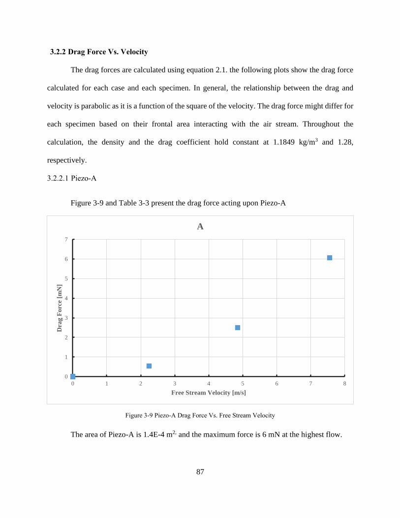
87
3.2.2 Drag Force Vs. Velocity
The drag forces are calculated using equation 2.1. the following plots show the drag force
calculated for each case and each specimen. In general, the relationship between the drag and
velocity is parabolic as it is a function of the square of the velocity. The drag force might differ for
each specimen based on their frontal area interacting with the air stream. Throughout the
calculation, the density and the drag coefficient hold constant at 1.1849 kg/m3 and 1.28,
respectively.
3.2.2.1 Piezo-A
Figure 3-9 and Table 3-3 present the drag force acting upon Piezo-A
The area of Piezo-A is 1.4E-4 m2, and the maximum force is 6 mN at the highest flow.
0
1
2
3
4
5
6
7
0 1 2 3 4 5 6 7 8
Dra
g F
orc
e [m
N]
Free Stream Velocity [m/s]
A
Figure 3-9 Piezo-A Drag Force Vs. Free Stream Velocity
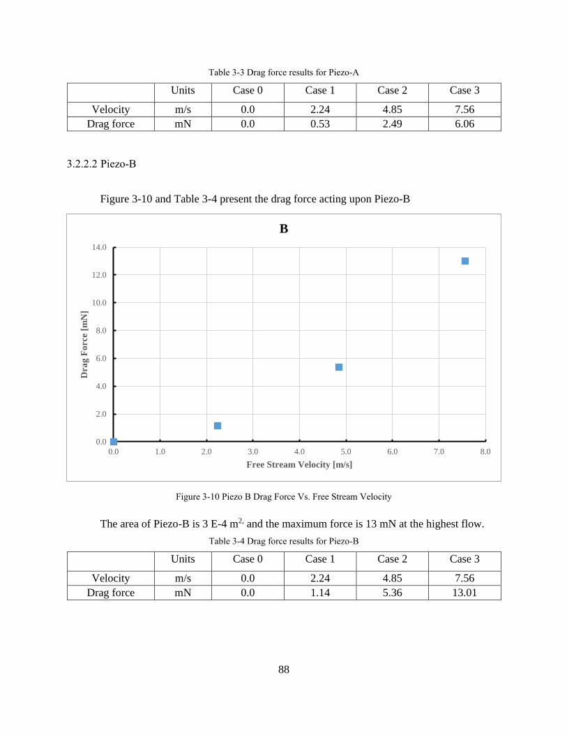
88
Table 3-3 Drag force results for Piezo-A
Units Case 0 Case 1 Case 2 Case 3
Velocity m/s 0.0 2.24 4.85 7.56
Drag force mN 0.0 0.53 2.49 6.06
3.2.2.2 Piezo-B
Figure 3-10 and Table 3-4 present the drag force acting upon Piezo-B
The area of Piezo-B is 3 E-4 m2, and the maximum force is 13 mN at the highest flow.
Table 3-4 Drag force results for Piezo-B
Units Case 0 Case 1 Case 2 Case 3
Velocity m/s 0.0 2.24 4.85 7.56
Drag force mN 0.0 1.14 5.36 13.01
0.0
2.0
4.0
6.0
8.0
10.0
12.0
14.0
0.0 1.0 2.0 3.0 4.0 5.0 6.0 7.0 8.0
Dra
g F
orc
e [m
N]
Free Stream Velocity [m/s]
B
Figure 3-10 Piezo B Drag Force Vs. Free Stream Velocity
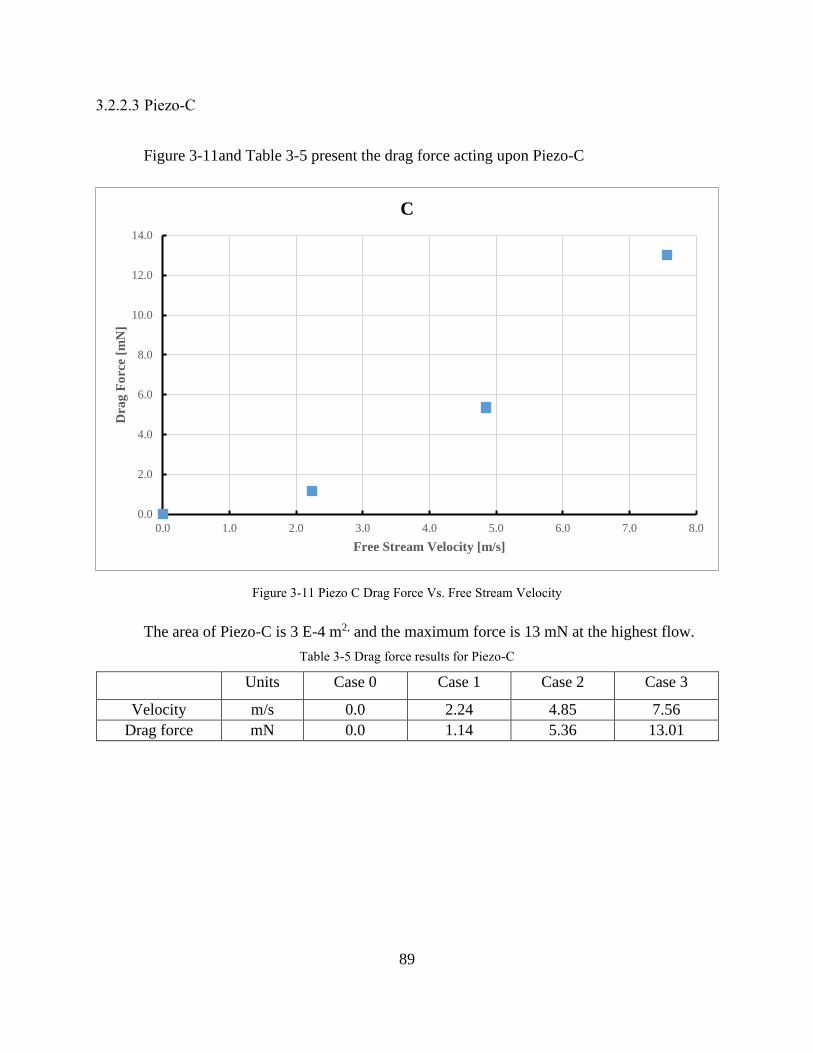
89
3.2.2.3 Piezo-C
Figure 3-11and Table 3-5 present the drag force acting upon Piezo-C
The area of Piezo-C is 3 E-4 m2, and the maximum force is 13 mN at the highest flow.
Table 3-5 Drag force results for Piezo-C
Units Case 0 Case 1 Case 2 Case 3
Velocity m/s 0.0 2.24 4.85 7.56
Drag force mN 0.0 1.14 5.36 13.01
0.0
2.0
4.0
6.0
8.0
10.0
12.0
14.0
0.0 1.0 2.0 3.0 4.0 5.0 6.0 7.0 8.0
Dra
g F
orc
e [m
N]
Free Stream Velocity [m/s]
C
Figure 3-11 Piezo C Drag Force Vs. Free Stream Velocity
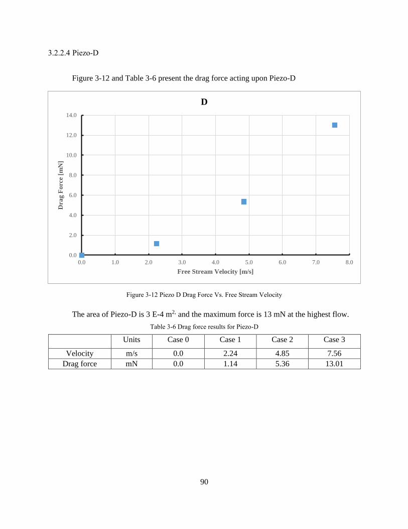
90
3.2.2.4 Piezo-D
Figure 3-12 and Table 3-6 present the drag force acting upon Piezo-D
The area of Piezo-D is 3 E-4 m2, and the maximum force is 13 mN at the highest flow.
Table 3-6 Drag force results for Piezo-D
Units Case 0 Case 1 Case 2 Case 3
Velocity m/s 0.0 2.24 4.85 7.56
Drag force mN 0.0 1.14 5.36 13.01
0.0
2.0
4.0
6.0
8.0
10.0
12.0
14.0
0.0 1.0 2.0 3.0 4.0 5.0 6.0 7.0 8.0
Dra
g F
orc
e [m
N]
Free Stream Velocity [m/s]
D
Figure 3-12 Piezo D Drag Force Vs. Free Stream Velocity
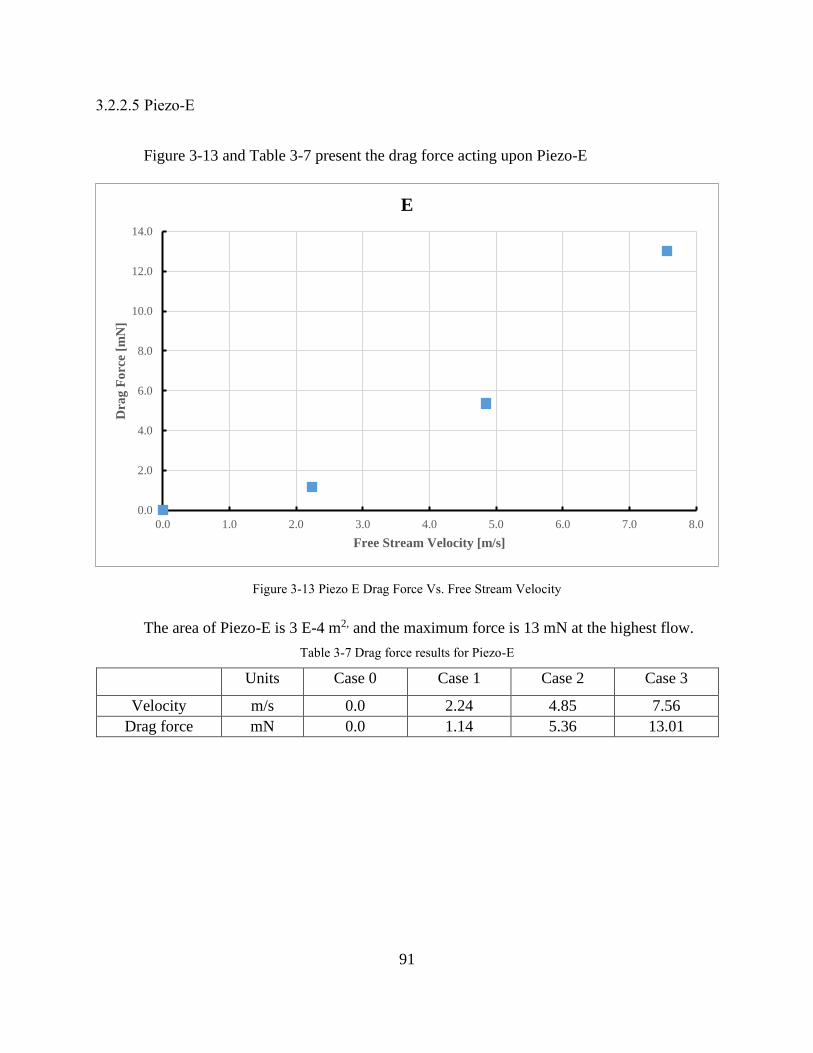
91
3.2.2.5 Piezo-E
Figure 3-13 and Table 3-7 present the drag force acting upon Piezo-E
The area of Piezo-E is 3 E-4 m2, and the maximum force is 13 mN at the highest flow.
Table 3-7 Drag force results for Piezo-E
Units Case 0 Case 1 Case 2 Case 3
Velocity m/s 0.0 2.24 4.85 7.56
Drag force mN 0.0 1.14 5.36 13.01
0.0
2.0
4.0
6.0
8.0
10.0
12.0
14.0
0.0 1.0 2.0 3.0 4.0 5.0 6.0 7.0 8.0
Dra
g F
orc
e [m
N]
Free Stream Velocity [m/s]
E
Figure 3-13 Piezo E Drag Force Vs. Free Stream Velocity
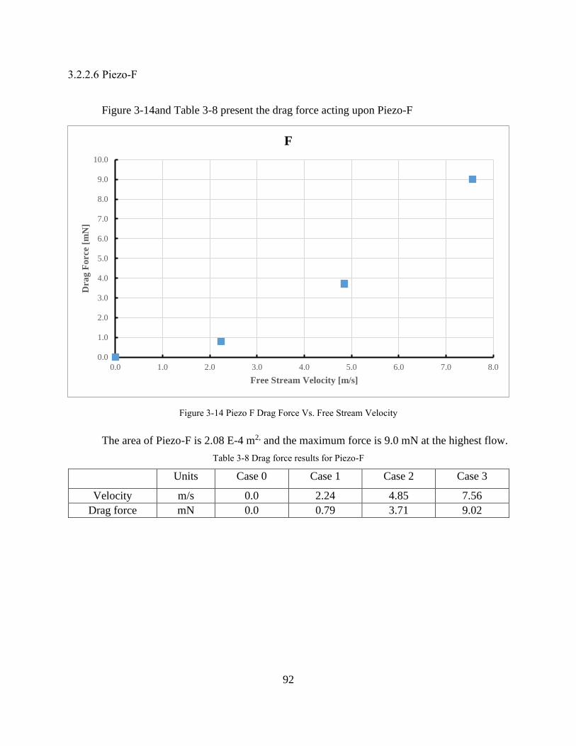
92
3.2.2.6 Piezo-F
Figure 3-14and Table 3-8 present the drag force acting upon Piezo-F
The area of Piezo-F is 2.08 E-4 m2, and the maximum force is 9.0 mN at the highest flow.
Table 3-8 Drag force results for Piezo-F
Units Case 0 Case 1 Case 2 Case 3
Velocity m/s 0.0 2.24 4.85 7.56
Drag force mN 0.0 0.79 3.71 9.02
0.0
1.0
2.0
3.0
4.0
5.0
6.0
7.0
8.0
9.0
10.0
0.0 1.0 2.0 3.0 4.0 5.0 6.0 7.0 8.0
Dra
g F
orc
e [m
N]
Free Stream Velocity [m/s]
F
Figure 3-14 Piezo F Drag Force Vs. Free Stream Velocity
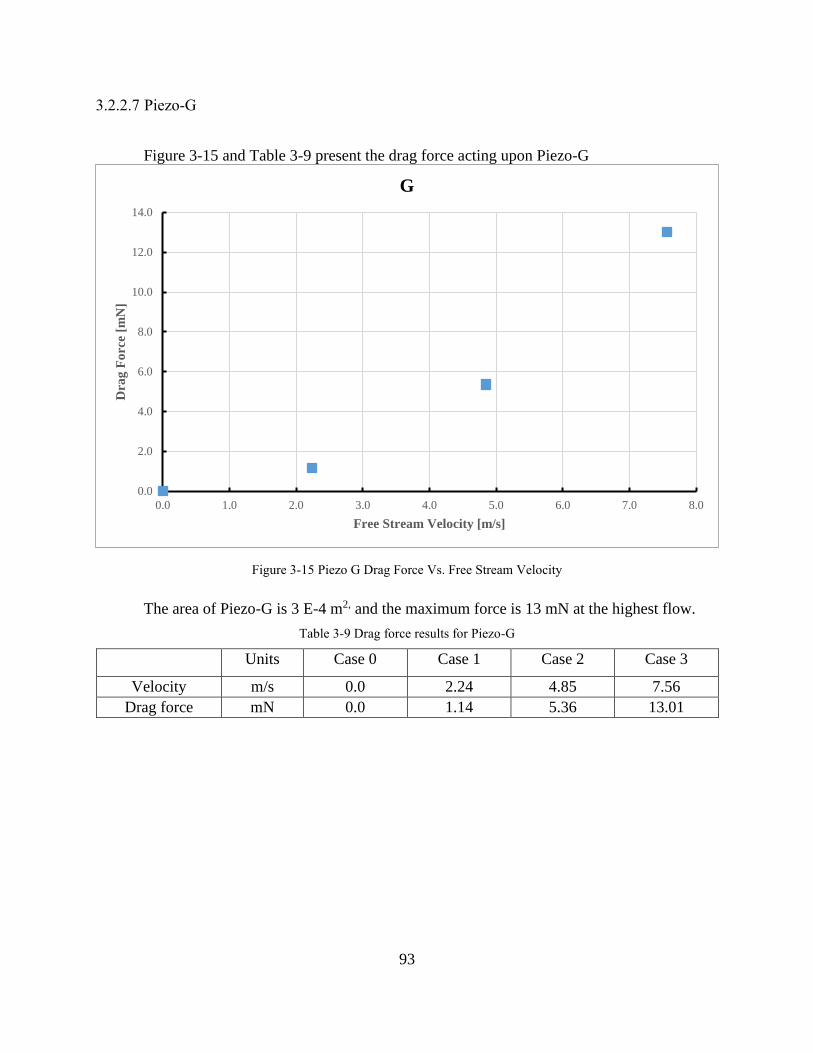
93
3.2.2.7 Piezo-G
Figure 3-15 and Table 3-9 present the drag force acting upon Piezo-G
The area of Piezo-G is 3 E-4 m2, and the maximum force is 13 mN at the highest flow.
Table 3-9 Drag force results for Piezo-G
Units Case 0 Case 1 Case 2 Case 3
Velocity m/s 0.0 2.24 4.85 7.56
Drag force mN 0.0 1.14 5.36 13.01
0.0
2.0
4.0
6.0
8.0
10.0
12.0
14.0
0.0 1.0 2.0 3.0 4.0 5.0 6.0 7.0 8.0
Dra
g F
orc
e [m
N]
Free Stream Velocity [m/s]
G
Figure 3-15 Piezo G Drag Force Vs. Free Stream Velocity
94
3.2.2.8 Piezo-H
Figure 3-16 and Table 3-10 present the drag force acting upon Piezo-H
The area of Piezo-H is 4.16 E-4 m2, and the maximum force is 18 mN at the highest flow.
Table 3-10 Drag force results for Piezo-H
Units Case 0 Case 1 Case 2 Case 3
Velocity m/s 0.0 2.24 4.85 7.56
Drag force mN 0.0 1.59 7.43 18.04
0.0
2.0
4.0
6.0
8.0
10.0
12.0
14.0
16.0
18.0
20.0
0.0 1.0 2.0 3.0 4.0 5.0 6.0 7.0 8.0
Dra
g F
orc
e [m
N]
Free Stream Velocity [m/s]
H
Figure 3-16 Piezo H Drag Force Vs. Free Stream Velocity
95
3.2.3 Voltage Output Vs. Drag Force
After exposure specimen to airflow, the signal collected was transferred to the root mean
square (RMS), as mentioned before. The RMS values were then averaged over the test time
duration and plotted against the drag force calculated previously.
3.2.3.1 Piezo-A
Figure 3-17 Piezo A Voltage Output Vs. Drag ForceFigure 3-17 and Table 3-11present the
voltage output due to drag force acting upon Piezo-A. The relationship between the voltage output
and drag force could be estimated as non-linear, where the voltage initially is increasing rapidly
then flat out near the maximum force.
The maximum voltage generated from Piezo-A is 3.46 mV at 6.06 mN of drag force.
Table 3-11 Drag force Vs. Voltage output results for Piezo-A
Units Case 0 Case 1 Case 2 Case 3
0.0
0.5
1.0
1.5
2.0
2.5
3.0
3.5
4.0
0.0 1.0 2.0 3.0 4.0 5.0 6.0 7.0
Vo
lta
ge
Ou
tpu
t [m
V]
Drag Force [mN]
A
Figure 3-17 Piezo A Voltage Output Vs. Drag Force
96
Drag force mN 0.00 0.53 2.49 6.06
Voltage mV 0.99 1.53 2.71 3.46
3.2.3.2 Piezo-B
Figure 3-18 and Table 3-12 present the voltage output due to drag force acting upon Piezo-
B. The relationship between the voltage output and drag force could be estimated as non-linear,
where the voltage initially dropped down below the reference value at no flow. This drop was
possibly caused by an error when the specimen was mounted as the clamps were tightened more
than the rest of the specimen, causing the reference value to be higher. After the air start flowing,
at case 1, the balanced forces resulted in lower voltage output. The voltage behaved similarly to
Piezo-A, where the voltage is increasing rapidly and then flat out near the maximum force. The
maximum voltage generated from Piezo-B is 4.75 mV at 13 mN of drag force.
Table 3-12 Drag force Vs. Voltage output results for Piezo-B
Units Case 0 Case 1 Case 2 Case 3
Drag force mN 0.00 1.14 5.36 13.01
0.0
1.0
2.0
3.0
4.0
5.0
6.0
0.0 2.0 4.0 6.0 8.0 10.0 12.0 14.0
Vo
lta
ge
Ou
tpu
t [m
V]
Drag Force [mN]
B
Figure 3-18 Piezo B Voltage Output Vs. Drag Force

97
Voltage mV 2.56 2.27 4.02 4.75
3.2.3.3 Piezo-C
Figure 3-19 and Table 3-13present the voltage output due to drag force acting upon Piezo-
C. The relationship between the voltage output and drag force could be estimated as non-linear,
where the voltage initially dropped down below the reference value at no flow. This drop was
possibly caused by an error when the specimen was mounted as the clamps were tightened harder,
causing the reference value to be higher. After the air start flowing, at case 1, the balanced forces
resulted in lower voltage output. The voltage behaved similarly to Piezo-A, where the voltage is
increasing rapidly and then flat out near the maximum force. The maximum voltage generated
from Piezo-C is 3.56 mV at 13 mN of drag force.
Table 3-13 Drag force Vs. Voltage output results for Piezo-C
Units Case 0 Case 1 Case 2 Case 3
Drag force mN 0.00 1.14 5.36 13.01
0.0
0.5
1.0
1.5
2.0
2.5
3.0
3.5
4.0
0.0 2.0 4.0 6.0 8.0 10.0 12.0 14.0
Vo
lta
ge
Ou
tpu
t [m
V]
Drag Force [mN]
C
Figure 3-19 Piezo C Voltage Output Vs. Drag Force
98
Voltage mV 2.08 1.88 2.47 3.59
3.2.3.4 Piezo-D
Figure 3-20 and Table 3-14 present the voltage output due to drag force acting upon Piezo-
D. The relationship between the voltage output and drag force could be estimated as non-linear,
where the voltage is initially increasing and then flat out near the maximum force.
The maximum voltage generated from Piezo-D is 6.43 mV at 13 mN of drag force
Table 3-14 Drag force Vs. Voltage output results for Piezo-D
Units Case 0 Case 1 Case 2 Case 3
Drag force mN 0.00 1.14 5.36 13.01
Voltage mV 2.95 3.23 4.65 6.43
0.0
1.0
2.0
3.0
4.0
5.0
6.0
7.0
0.0 2.0 4.0 6.0 8.0 10.0 12.0 14.0
Vo
lta
ge
Ou
tpu
t [m
V[
Drag Force [mN]
D
Figure 3-20 Piezo D Voltage Output Vs. Drag Force

99
3.2.3.5 Piezo-E
Figure 3-21 and Table 3-15 present the voltage output due to drag force acting upon Piezo-
E. The relationship between the voltage output and drag force could be estimated as non-linear,
where the voltage is initially increasing and then flat out near the maximum force.
The maximum voltage generated from Piezo-E is 18.03 mV at 13 mN of drag force
Table 3-15 Drag force Vs. Voltage output results for Piezo-E
Units Case 0 Case 1 Case 2 Case 3
Drag force mN 0.00 1.14 5.36 13.01
Voltage mV 3.53 8.05 14.12 18.03
0.0
2.0
4.0
6.0
8.0
10.0
12.0
14.0
16.0
18.0
20.0
0.0 2.0 4.0 6.0 8.0 10.0 12.0 14.0
Vo
lta
ge
Ou
tpu
t [m
V]
Drag Force [mN]
E
Figure 3-21 Piezo E Voltage Output Vs. Drag Force

100
3.2.3.6 Piezo-F
Figure 3-22 and Table 3-16 present the voltage output due to drag force acting upon Piezo-
F. The relationship between the voltage output and drag force could be estimated as non-linear,
where the voltage is initially increasing and then flat out near the maximum force
The maximum voltage generated from Piezo-E is 4.41 mV at 9.02 mN of drag force
Table 3-16 Drag force Vs. Voltage output results for Piezo-F
Units Case 0 Case 1 Case 2 Case 3
Drag force mN 0.00 0.79 3.71 9.02
Voltage mV 1.52 2.18 3.89 4.41
0.0
0.5
1.0
1.5
2.0
2.5
3.0
3.5
4.0
4.5
5.0
0.0 1.0 2.0 3.0 4.0 5.0 6.0 7.0 8.0 9.0 10.0
Vo
lta
ge
Ou
tpu
t [m
V]
Drag Force [mN
F
Figure 3-22 Piezo F Voltage Output Vs. Drag Force
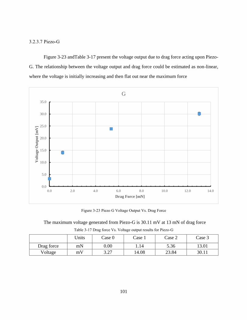
101
3.2.3.7 Piezo-G
Figure 3-23 andTable 3-17 present the voltage output due to drag force acting upon Piezo-
G. The relationship between the voltage output and drag force could be estimated as non-linear,
where the voltage is initially increasing and then flat out near the maximum force
The maximum voltage generated from Piezo-G is 30.11 mV at 13 mN of drag force
Table 3-17 Drag force Vs. Voltage output results for Piezo-G
Units Case 0 Case 1 Case 2 Case 3
Drag force mN 0.00 1.14 5.36 13.01
Voltage mV 3.27 14.08 23.84 30.11
0.0
5.0
10.0
15.0
20.0
25.0
30.0
35.0
0.0 2.0 4.0 6.0 8.0 10.0 12.0 14.0
Vo
lta
ge
Ou
tpu
t [m
V]
Drag Force [mN]
G
Figure 3-23 Piezo G Voltage Output Vs. Drag Force
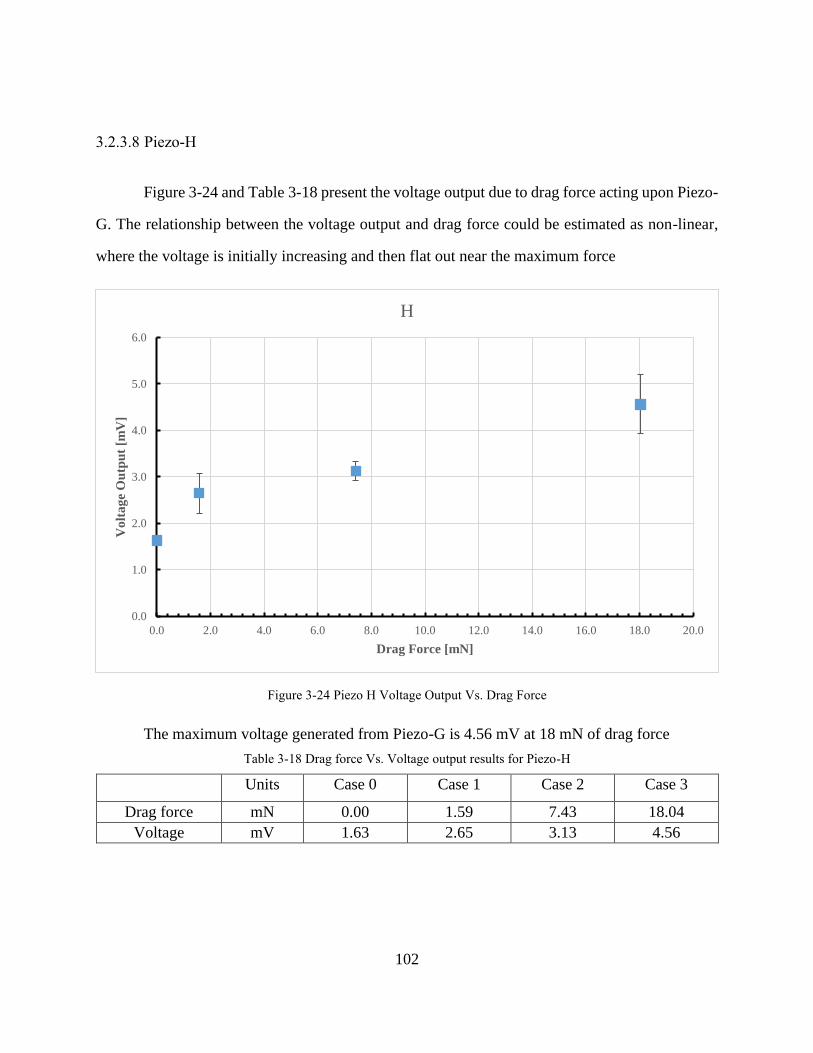
102
3.2.3.8 Piezo-H
Figure 3-24 and Table 3-18 present the voltage output due to drag force acting upon Piezo-
G. The relationship between the voltage output and drag force could be estimated as non-linear,
where the voltage is initially increasing and then flat out near the maximum force
The maximum voltage generated from Piezo-G is 4.56 mV at 18 mN of drag force
Table 3-18 Drag force Vs. Voltage output results for Piezo-H
Units Case 0 Case 1 Case 2 Case 3
Drag force mN 0.00 1.59 7.43 18.04
Voltage mV 1.63 2.65 3.13 4.56
0.0
1.0
2.0
3.0
4.0
5.0
6.0
0.0 2.0 4.0 6.0 8.0 10.0 12.0 14.0 16.0 18.0 20.0
Vo
lta
ge
Ou
tpu
t [m
V]
Drag Force [mN]
H
Figure 3-24 Piezo H Voltage Output Vs. Drag Force
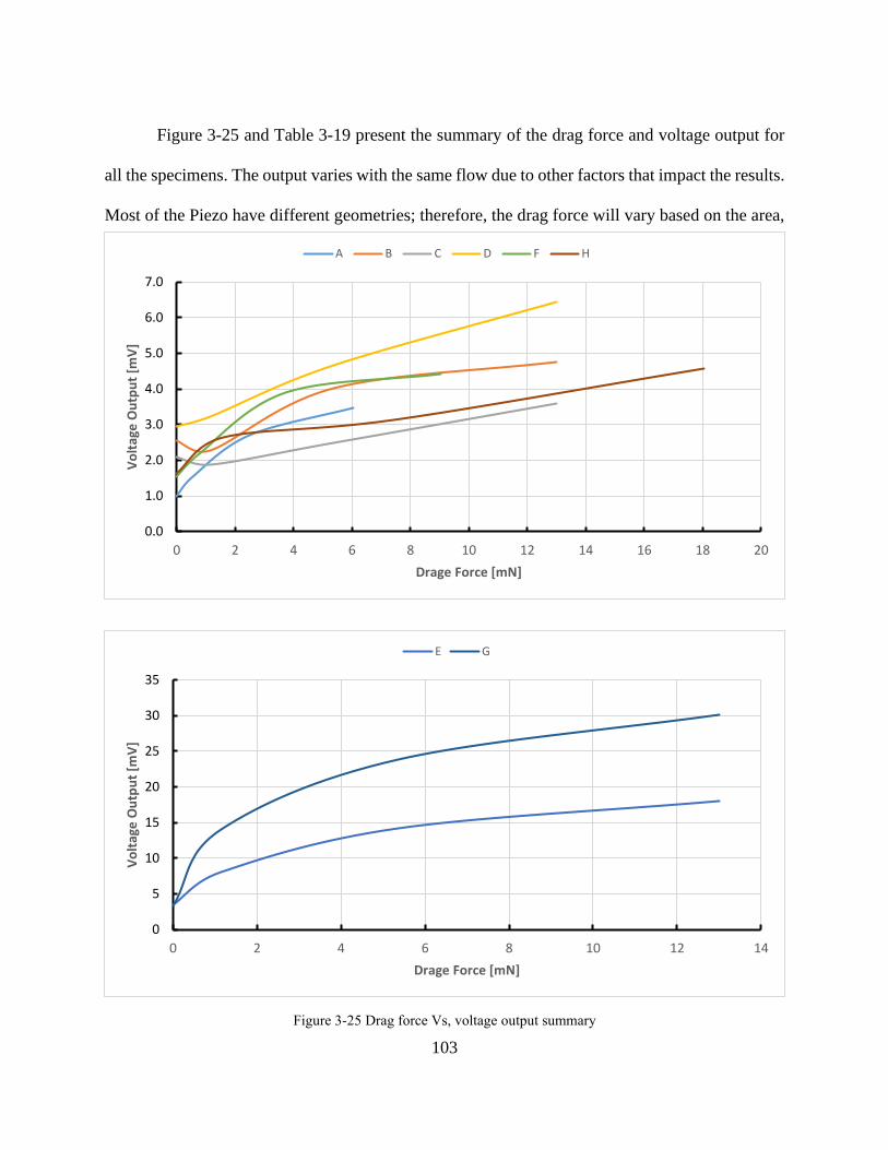
103
Figure 3-25 and Table 3-19 present the summary of the drag force and voltage output for
all the specimens. The output varies with the same flow due to other factors that impact the results.
Most of the Piezo have different geometries; therefore, the drag force will vary based on the area,
0.0
1.0
2.0
3.0
4.0
5.0
6.0
7.0
0 2 4 6 8 10 12 14 16 18 20
Vo
ltag
e O
utp
ut
[mV
]
Drage Force [mN]
A B C D F H
0
5
10
15
20
25
30
35
0 2 4 6 8 10 12 14
Vo
ltag
e O
utp
ut
[mV
]
Drage Force [mN]
E G
Figure 3-25 Drag force Vs, voltage output summary

104
thickness, length, and width. Piezo B, C, D, E, and G have the same area but differ in thickness,
and Piezo-G has different length and width. As a reason, the voltage was very different even when
the force was constant. This part will be explained later in this study.
Table 3-19 Drag force and voltage output summary
Case 0 Case 1 Case 2 Case 3
mN mV mN mV mN mV mN mV
A 0.00 0.99 0.53 1.53 2.49 2.71 6.06 3.46
B 0.00 2.56 1.14 2.27 5.36 4.02 13.01 4.75
C 0.00 2.08 1.14 1.88 5.36 2.47 13.01 3.59
D 0.00 2.95 1.14 3.23 5.36 4.65 13.01 6.43
E 0.00 3.53 1.14 8.05 5.36 14.12 13.01 18.03
F 0.00 1.52 0.79 2.18 3.71 3.89 9.02 4.41
G 0.00 3.27 1.14 14.08 5.36 23.84 13.01 30.11
H 0.00 1.63 1.59 2.65 7.43 3.13 18.04 4.56

105
3.2.4 Voltage Output Vs. Flow Rate
The flow meter design needs to map the change in the flow rate and the resulting voltage.
Therefore, it is essential to see the overall relationship between flow rate and voltage output.
The following sections show the average voltage over the test cases with a statistical study
and its relationship with change in the flow rate. A curve fit method was also used to approximate
an equation used to predict the voltage output for unknown flow rates. A sigmoid curve fit with
four constants was used to estimate the best curve fit, as shown in equation 3.1. SigmaPlot software
was used to calculate the coefficients.
The sigmoid curve fit was chosen as it represents a realistic scenario with lower and upper
limits where the sensor response would be constant.
3.2.4.1 Piezo-A
Figure 3-26 presents the voltage output due to a change in the flow rate for Piezo-A. The
relationship between the voltage output and the flow rate could be estimated as non-linear. The
voltage is initially increasing flat out near the maximum flow rate forming an S curve.
𝑦 = 𝑦0 +𝑎
1 + 𝑒−(𝑥−𝑥0𝑏
)
3.1
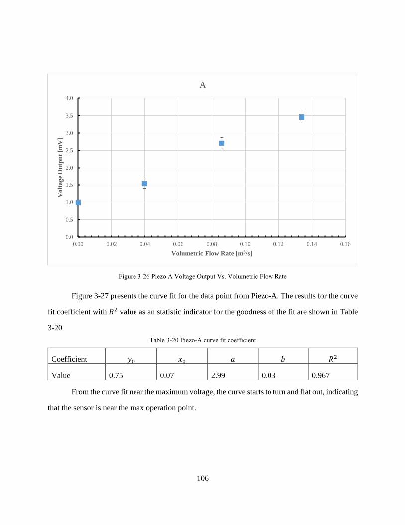
106
Figure 3-27 presents the curve fit for the data point from Piezo-A. The results for the curve
fit coefficient with 𝑅2 value as an statistic indicator for the goodness of the fit are shown in Table
3-20
Table 3-20 Piezo-A curve fit coefficient
Coefficient 𝑦0 𝑥0 𝑎 𝑏 𝑅2
Value 0.75 0.07 2.99 0.03 0.967
From the curve fit near the maximum voltage, the curve starts to turn and flat out, indicating
that the sensor is near the max operation point.
0.0
0.5
1.0
1.5
2.0
2.5
3.0
3.5
4.0
0.00 0.02 0.04 0.06 0.08 0.10 0.12 0.14 0.16
Vo
lta
ge
Ou
tpu
t [m
V]
Volumetric Flow Rate [m3/s]
A
Figure 3-26 Piezo A Voltage Output Vs. Volumetric Flow Rate
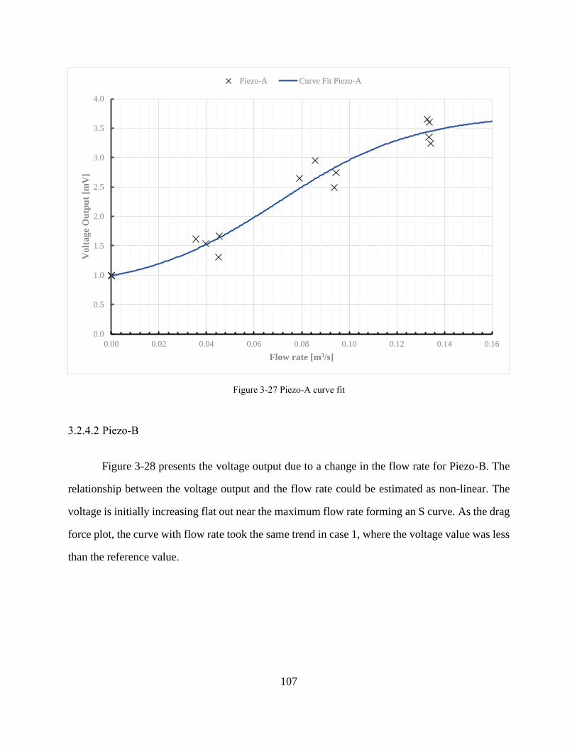
107
3.2.4.2 Piezo-B
Figure 3-28 presents the voltage output due to a change in the flow rate for Piezo-B. The
relationship between the voltage output and the flow rate could be estimated as non-linear. The
voltage is initially increasing flat out near the maximum flow rate forming an S curve. As the drag
force plot, the curve with flow rate took the same trend in case 1, where the voltage value was less
than the reference value.
0.0
0.5
1.0
1.5
2.0
2.5
3.0
3.5
4.0
0.00 0.02 0.04 0.06 0.08 0.10 0.12 0.14 0.16
Vo
lta
ge
Ou
tpu
t [m
V]
Flow rate [m3/s]
Piezo-A Curve Fit Piezo-A
Figure 3-27 Piezo-A curve fit
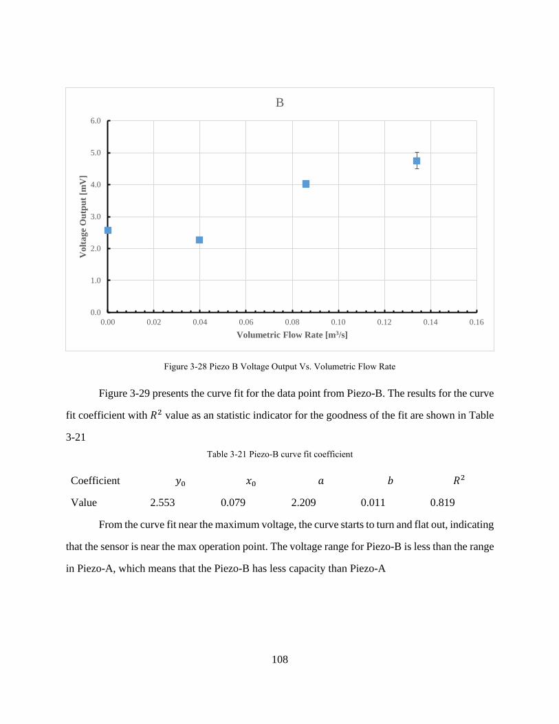
108
Figure 3-29 presents the curve fit for the data point from Piezo-B. The results for the curve
fit coefficient with 𝑅2 value as an statistic indicator for the goodness of the fit are shown in Table
3-21
Table 3-21 Piezo-B curve fit coefficient
Coefficient 𝑦0 𝑥0 𝑎 𝑏 𝑅2
Value 2.553 0.079 2.209 0.011 0.819
From the curve fit near the maximum voltage, the curve starts to turn and flat out, indicating
that the sensor is near the max operation point. The voltage range for Piezo-B is less than the range
in Piezo-A, which means that the Piezo-B has less capacity than Piezo-A
0.0
1.0
2.0
3.0
4.0
5.0
6.0
0.00 0.02 0.04 0.06 0.08 0.10 0.12 0.14 0.16
Vo
lta
ge
Ou
tpu
t [m
V]
Volumetric Flow Rate [m3/s]
B
Figure 3-28 Piezo B Voltage Output Vs. Volumetric Flow Rate
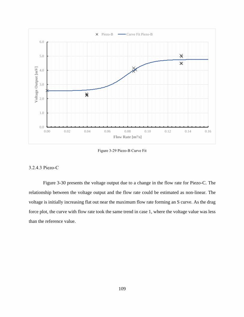
109
3.2.4.3 Piezo-C
Figure 3-30 presents the voltage output due to a change in the flow rate for Piezo-C. The
relationship between the voltage output and the flow rate could be estimated as non-linear. The
voltage is initially increasing flat out near the maximum flow rate forming an S curve. As the drag
force plot, the curve with flow rate took the same trend in case 1, where the voltage value was less
than the reference value.
0.0
1.0
2.0
3.0
4.0
5.0
6.0
0.00 0.02 0.04 0.06 0.08 0.10 0.12 0.14 0.16
Vo
lta
ge
Ou
tpu
t [m
V]
Flow Rate [m3/s]
Piezo-B Curve Fit Piezo-B
Figure 3-29 Piezo-B Curve Fit
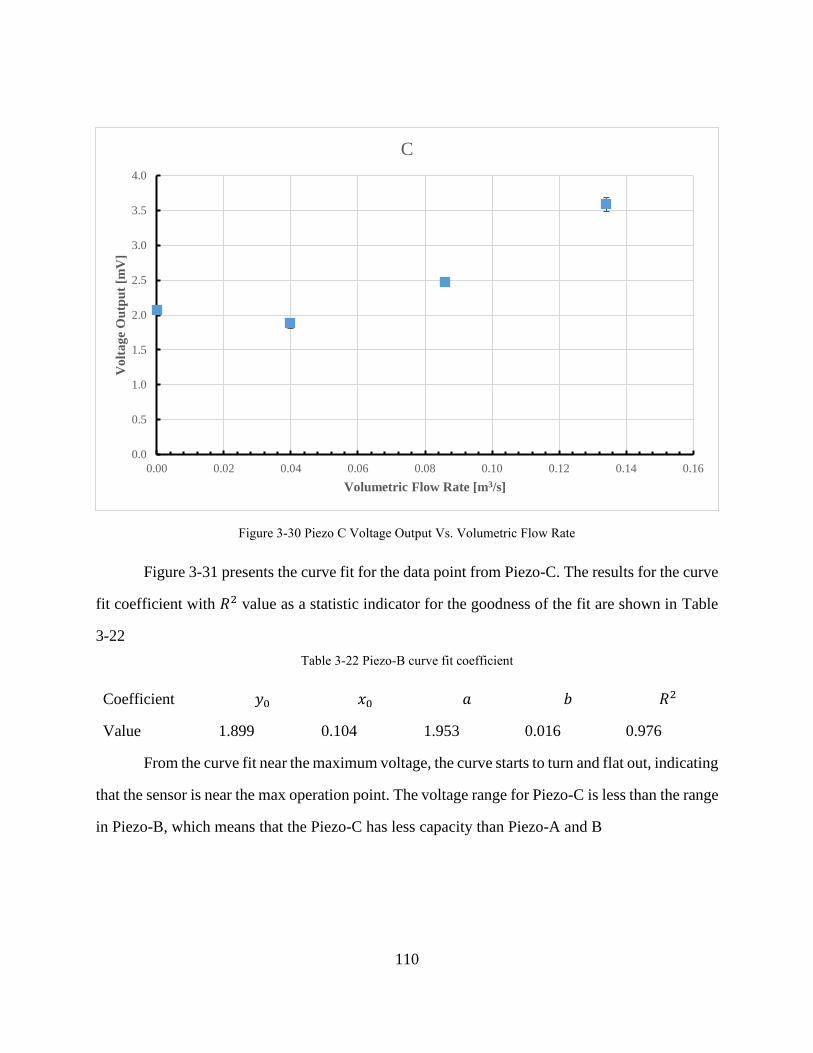
110
Figure 3-31 presents the curve fit for the data point from Piezo-C. The results for the curve
fit coefficient with 𝑅2 value as a statistic indicator for the goodness of the fit are shown in Table
3-22
Table 3-22 Piezo-B curve fit coefficient
Coefficient 𝑦0 𝑥0 𝑎 𝑏 𝑅2
Value 1.899 0.104 1.953 0.016 0.976
From the curve fit near the maximum voltage, the curve starts to turn and flat out, indicating
that the sensor is near the max operation point. The voltage range for Piezo-C is less than the range
in Piezo-B, which means that the Piezo-C has less capacity than Piezo-A and B
0.0
0.5
1.0
1.5
2.0
2.5
3.0
3.5
4.0
0.00 0.02 0.04 0.06 0.08 0.10 0.12 0.14 0.16
Vo
lta
ge
Ou
tpu
t [m
V]
Volumetric Flow Rate [m3/s]
C
Figure 3-30 Piezo C Voltage Output Vs. Volumetric Flow Rate
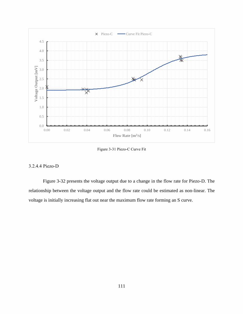
111
3.2.4.4 Piezo-D
Figure 3-32 presents the voltage output due to a change in the flow rate for Piezo-D. The
relationship between the voltage output and the flow rate could be estimated as non-linear. The
voltage is initially increasing flat out near the maximum flow rate forming an S curve.
0.0
0.5
1.0
1.5
2.0
2.5
3.0
3.5
4.0
4.5
0.00 0.02 0.04 0.06 0.08 0.10 0.12 0.14 0.16
Vo
lta
ge
Ou
tpu
t [m
V]
Flow Rate [m3/s]
Piezo-C Curve Fit Piezo-C
Figure 3-31 Piezo-C Curve Fit
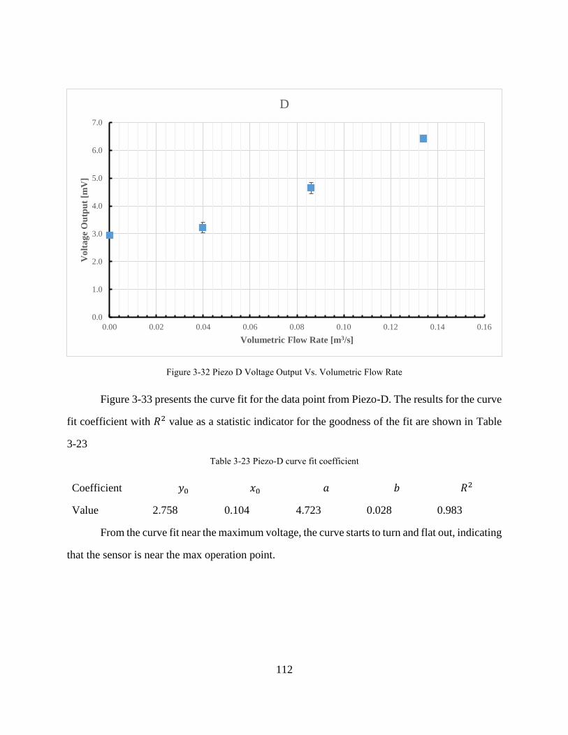
112
Figure 3-33 presents the curve fit for the data point from Piezo-D. The results for the curve
fit coefficient with 𝑅2 value as a statistic indicator for the goodness of the fit are shown in Table
3-23
Table 3-23 Piezo-D curve fit coefficient
Coefficient 𝑦0 𝑥0 𝑎 𝑏 𝑅2
Value 2.758 0.104 4.723 0.028 0.983
From the curve fit near the maximum voltage, the curve starts to turn and flat out, indicating
that the sensor is near the max operation point.
0.0
1.0
2.0
3.0
4.0
5.0
6.0
7.0
0.00 0.02 0.04 0.06 0.08 0.10 0.12 0.14 0.16
Vo
lta
ge
Ou
tpu
t [m
V]
Volumetric Flow Rate [m3/s]
D
Figure 3-32 Piezo D Voltage Output Vs. Volumetric Flow Rate

113
3.2.4.5 Piezo-E
Figure 3-34presents the voltage output due to a change in the flow rate for Piezo-E. The
relationship between the voltage output and the flow rate could be estimated as non-linear. The
voltage is initially increasing flat out near the maximum flow rate forming an S curve.
0.0
1.0
2.0
3.0
4.0
5.0
6.0
7.0
8.0
0.00 0.02 0.04 0.06 0.08 0.10 0.12 0.14 0.16
Vo
lta
ge
Ou
tpu
t [m
V]
Flow Rate [m3/s]
Piezo-D Curve Fit Piezo-D
Figure 3-33 Piezo-D Curve Fit
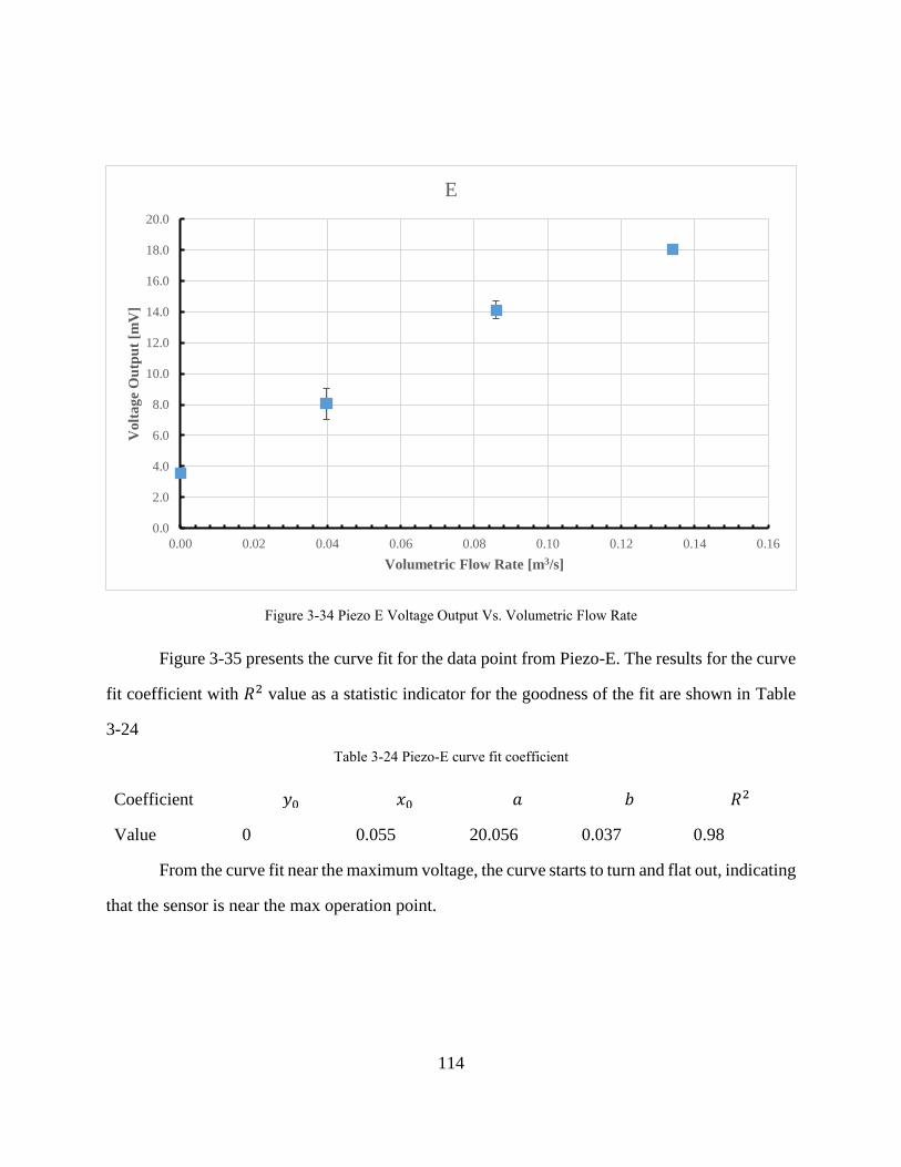
114
Figure 3-35 presents the curve fit for the data point from Piezo-E. The results for the curve
fit coefficient with 𝑅2 value as a statistic indicator for the goodness of the fit are shown in Table
3-24
Table 3-24 Piezo-E curve fit coefficient
Coefficient 𝑦0 𝑥0 𝑎 𝑏 𝑅2
Value 0 0.055 20.056 0.037 0.98
From the curve fit near the maximum voltage, the curve starts to turn and flat out, indicating
that the sensor is near the max operation point.
0.0
2.0
4.0
6.0
8.0
10.0
12.0
14.0
16.0
18.0
20.0
0.00 0.02 0.04 0.06 0.08 0.10 0.12 0.14 0.16
Vo
lta
ge
Ou
tpu
t [m
V]
Volumetric Flow Rate [m3/s]
E
Figure 3-34 Piezo E Voltage Output Vs. Volumetric Flow Rate
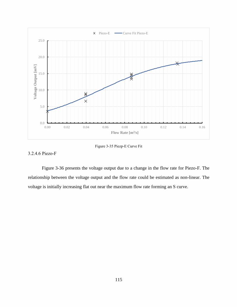
115
3.2.4.6 Piezo-F
Figure 3-36 presents the voltage output due to a change in the flow rate for Piezo-F. The
relationship between the voltage output and the flow rate could be estimated as non-linear. The
voltage is initially increasing flat out near the maximum flow rate forming an S curve.
0.0
5.0
10.0
15.0
20.0
25.0
0.00 0.02 0.04 0.06 0.08 0.10 0.12 0.14 0.16
Vo
lta
ge
Ou
tpu
t [m
V]
Flow Rate [m3/s]
Piezo-E Curve Fit Piezo-E
Figure 3-35 Piezp-E Curve Fit
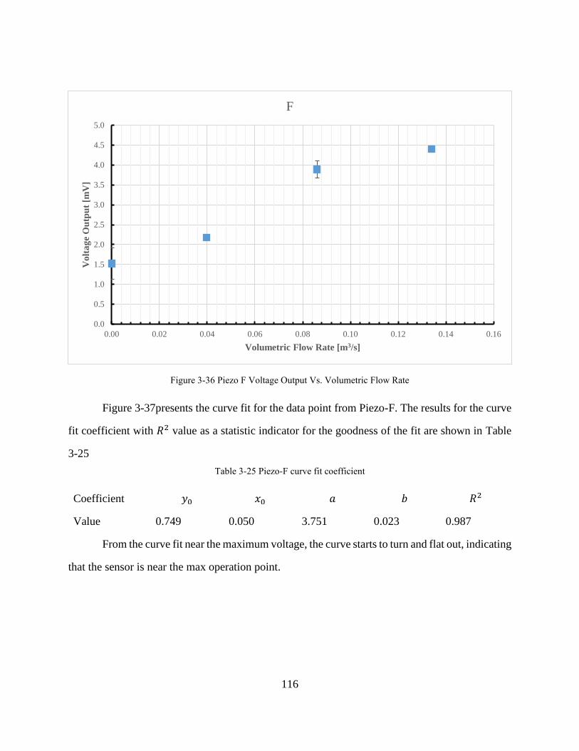
116
Figure 3-37presents the curve fit for the data point from Piezo-F. The results for the curve
fit coefficient with 𝑅2 value as a statistic indicator for the goodness of the fit are shown in Table
3-25
Table 3-25 Piezo-F curve fit coefficient
Coefficient 𝑦0 𝑥0 𝑎 𝑏 𝑅2
Value 0.749 0.050 3.751 0.023 0.987
From the curve fit near the maximum voltage, the curve starts to turn and flat out, indicating
that the sensor is near the max operation point.
0.0
0.5
1.0
1.5
2.0
2.5
3.0
3.5
4.0
4.5
5.0
0.00 0.02 0.04 0.06 0.08 0.10 0.12 0.14 0.16
Vo
lta
ge
Ou
tpu
t [m
V]
Volumetric Flow Rate [m3/s]
F
Figure 3-36 Piezo F Voltage Output Vs. Volumetric Flow Rate
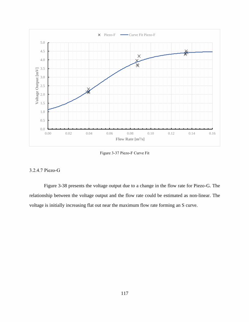
117
3.2.4.7 Piezo-G
Figure 3-38 presents the voltage output due to a change in the flow rate for Piezo-G. The
relationship between the voltage output and the flow rate could be estimated as non-linear. The
voltage is initially increasing flat out near the maximum flow rate forming an S curve.
0.0
0.5
1.0
1.5
2.0
2.5
3.0
3.5
4.0
4.5
5.0
0.00 0.02 0.04 0.06 0.08 0.10 0.12 0.14 0.16
Vo
lta
ge
Ou
tpu
t [m
V]
Flow Rate [m3/s]
Piezo-F Curve Fit Piezo-F
Figure 3-37 Piezo-F Curve Fit
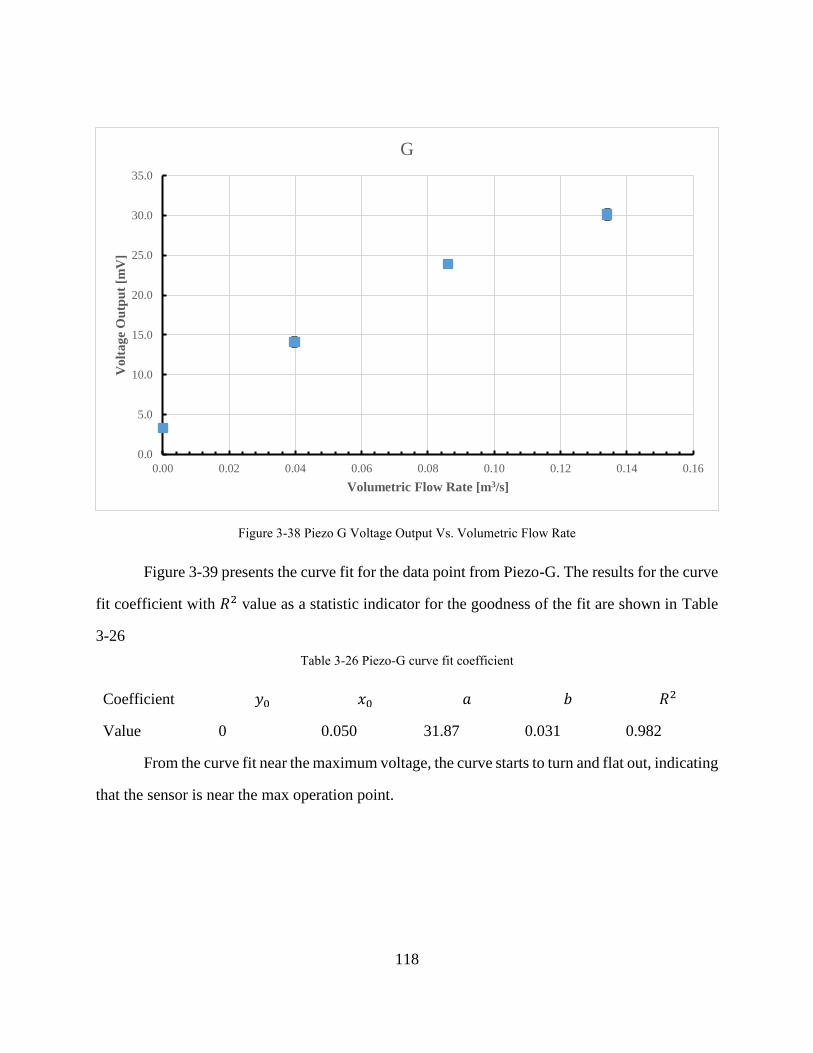
118
Figure 3-39 presents the curve fit for the data point from Piezo-G. The results for the curve
fit coefficient with 𝑅2 value as a statistic indicator for the goodness of the fit are shown in Table
3-26
Table 3-26 Piezo-G curve fit coefficient
Coefficient 𝑦0 𝑥0 𝑎 𝑏 𝑅2
Value 0 0.050 31.87 0.031 0.982
From the curve fit near the maximum voltage, the curve starts to turn and flat out, indicating
that the sensor is near the max operation point.
0.0
5.0
10.0
15.0
20.0
25.0
30.0
35.0
0.00 0.02 0.04 0.06 0.08 0.10 0.12 0.14 0.16
Vo
lta
ge
Ou
tpu
t [m
V]
Volumetric Flow Rate [m3/s]
G
Figure 3-38 Piezo G Voltage Output Vs. Volumetric Flow Rate
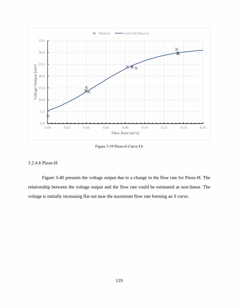
119
3.2.4.8 Piezo-H
Figure 3-40 presents the voltage output due to a change in the flow rate for Piezo-H. The
relationship between the voltage output and the flow rate could be estimated as non-linear. The
voltage is initially increasing flat out near the maximum flow rate forming an S curve.
0.0
5.0
10.0
15.0
20.0
25.0
30.0
35.0
0.00 0.02 0.04 0.06 0.08 0.10 0.12 0.14 0.16
Vo
lta
ge
Ou
tpu
t [m
V]
Flow Rate [m3/s]
Piezo-G Curve Fit Piezo-G
Figure 3-39 Piezo-G Curve Fit
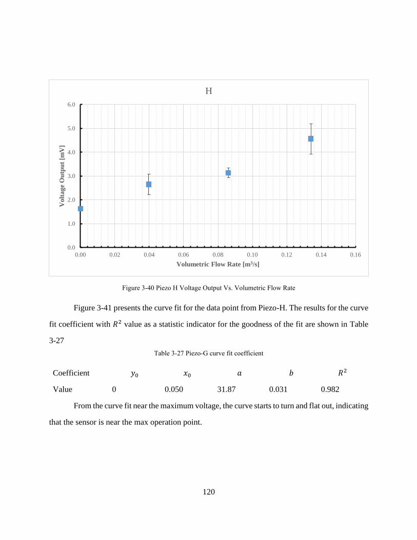
120
Figure 3-41 presents the curve fit for the data point from Piezo-H. The results for the curve
fit coefficient with 𝑅2 value as a statistic indicator for the goodness of the fit are shown in Table
3-27
Table 3-27 Piezo-G curve fit coefficient
Coefficient 𝑦0 𝑥0 𝑎 𝑏 𝑅2
Value 0 0.050 31.87 0.031 0.982
From the curve fit near the maximum voltage, the curve starts to turn and flat out, indicating
that the sensor is near the max operation point.
0.0
1.0
2.0
3.0
4.0
5.0
6.0
0.00 0.02 0.04 0.06 0.08 0.10 0.12 0.14 0.16
Vo
lta
ge
Ou
tpu
t [m
V]
Volumetric Flow Rate [m3/s]
H
Figure 3-40 Piezo H Voltage Output Vs. Volumetric Flow Rate
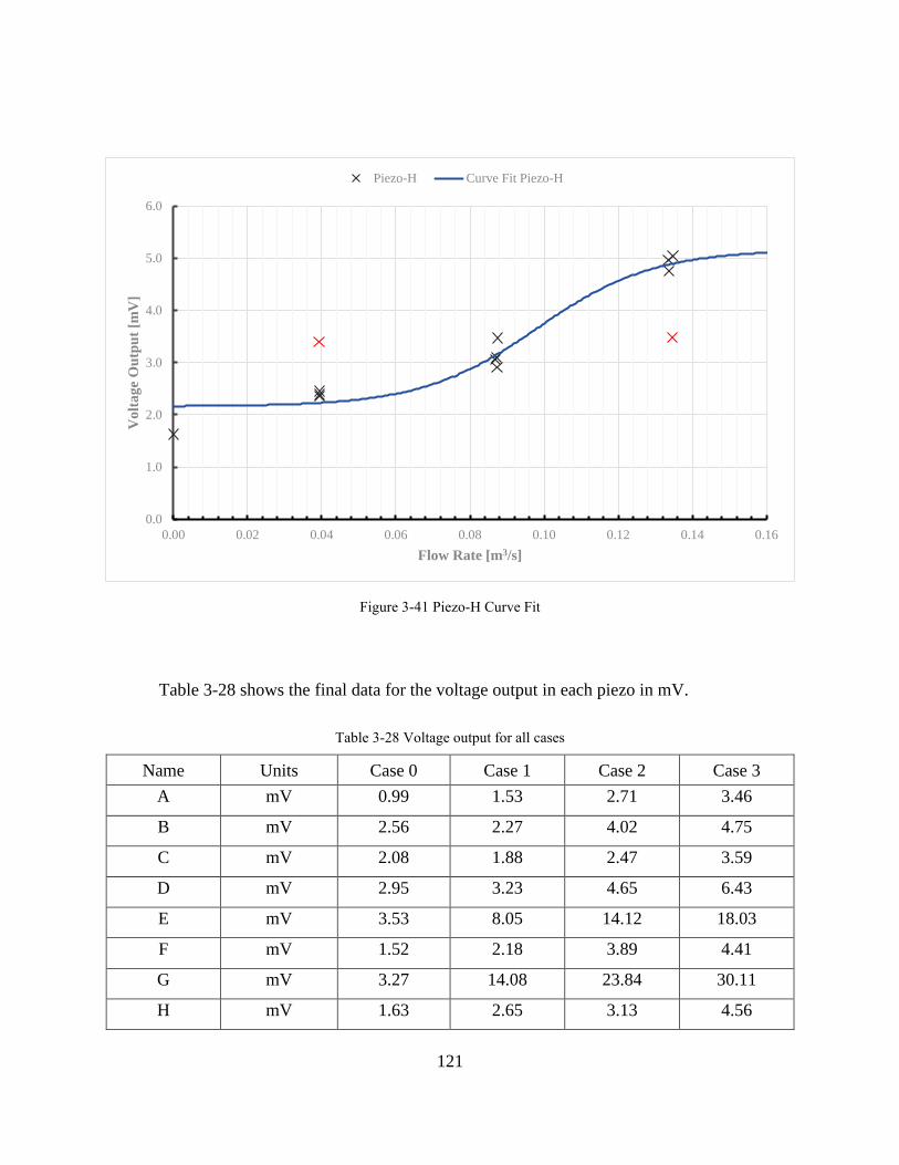
121
Table 3-28 shows the final data for the voltage output in each piezo in mV.
Table 3-28 Voltage output for all cases
Name Units Case 0 Case 1 Case 2 Case 3
A mV 0.99 1.53 2.71 3.46
B mV 2.56 2.27 4.02 4.75
C mV 2.08 1.88 2.47 3.59
D mV 2.95 3.23 4.65 6.43
E mV 3.53 8.05 14.12 18.03
F mV 1.52 2.18 3.89 4.41
G mV 3.27 14.08 23.84 30.11
H mV 1.63 2.65 3.13 4.56
0.0
1.0
2.0
3.0
4.0
5.0
6.0
0.00 0.02 0.04 0.06 0.08 0.10 0.12 0.14 0.16
Vo
lta
ge
Ou
tpu
t [m
V]
Flow Rate [m3/s]
Piezo-H Curve Fit Piezo-H
Figure 3-41 Piezo-H Curve Fit
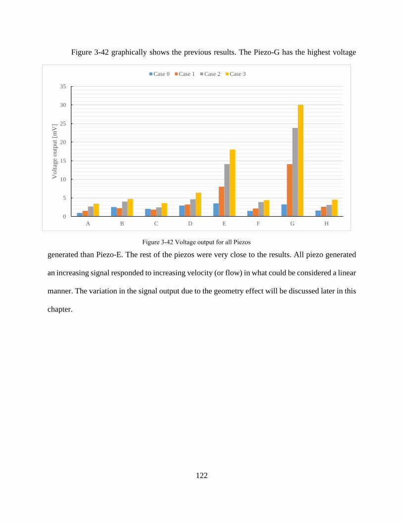
122
Figure 3-42 graphically shows the previous results. The Piezo-G has the highest voltage
generated than Piezo-E. The rest of the piezos were very close to the results. All piezo generated
an increasing signal responded to increasing velocity (or flow) in what could be considered a linear
manner. The variation in the signal output due to the geometry effect will be discussed later in this
chapter.
0
5
10
15
20
25
30
35
A B C D E F G H
Vo
ltag
e o
utp
ut
[mV
]
Case 0 Case 1 Case 2 Case 3
Figure 3-42 Voltage output for all Piezos
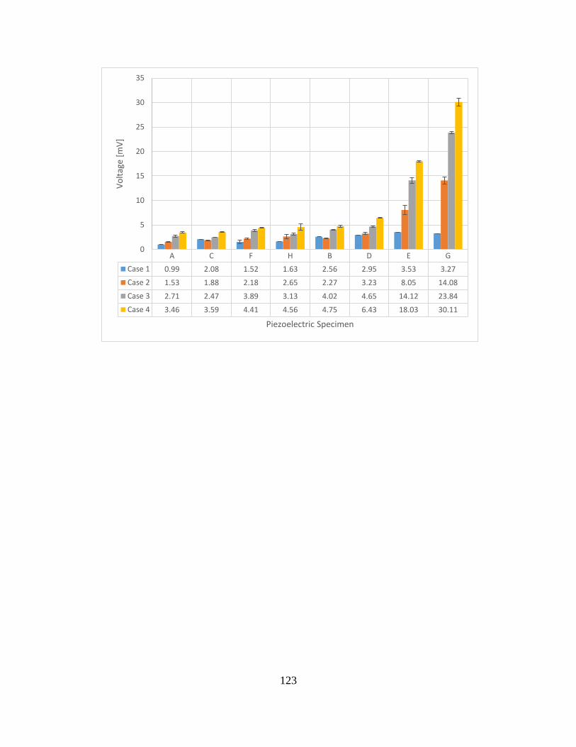
123
A C F H B D E G
Case 1 0.99 2.08 1.52 1.63 2.56 2.95 3.53 3.27
Case 2 1.53 1.88 2.18 2.65 2.27 3.23 8.05 14.08
Case 3 2.71 2.47 3.89 3.13 4.02 4.65 14.12 23.84
Case 4 3.46 3.59 4.41 4.56 4.75 6.43 18.03 30.11
0
5
10
15
20
25
30
35
Vo
ltag
e [m
V]
Piezoelectric Specimen
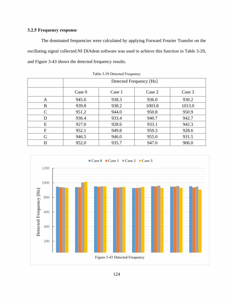
124
3.2.5 Frequency response
The dominated frequencies were calculated by applying Forward Fourier Transfer on the
oscillating signal collected.NI DIAdem software was used to achieve this function in Table 3-29,
and Figure 3-43 shows the detected frequency results.
Table 3-29 Detected Frequency
Detected Frequency [Hz]
Case 0 Case 1 Case 2 Case 3
A 945.6 938.3 936.0 930.2
B 939.8 938.2 1003.8 1013.0
C 951.2 944.0 950.8 950.9
D 936.4 933.4 940.7 942.7
E 927.0 928.6 933.1 942.3
F 952.1 949.8 959.3 928.6
G 946.5 946.0 955.0 931.5
H 952.0 935.7 947.0 906.0
0
200
400
600
800
1000
1200
Det
ecte
d F
req
uen
cy [
Hz]
Case 0 Case 1 Case 2 Case 3
Figure 3-43 Detected Frequency

125
The detected frequency for each Piezo is similar, which means that the system responds in
the same frequency regarding the Piezo specimen inserted in it. As a reason, the system considers
stable.
3.2.6 Signal to noise ratio
SNR's importance is showing the signal's quality; the higher the ratio, the better signal.
Defining noise is a significant concern for all signal outputs, becoming overly complicated and
changing this study's focus. As a reason, the noise for this study is defined as a signal collected
when airflow is at 0. This noise is estimated to have most of the external and internal noise. Table
3-30 and Figure 3-44 shows how the signal to noise ratio (SNR) for each state voltage output. The
SNR is calculated from equation (1.28) in dB.
The SRN is increasing for each case, which leads to better signal over noise. The SNR
shows the same pattern as the voltage output where Piezo-G has the highest SNR, then Piezo-E
and the rest had similar ratios.
Table 3-30 Signal to Noise Ratio (SNR)
SNR
Case 1 Case 2 Case 3
A 3.79 8.75 10.88
B -1.06 3.91 5.36
C -0.86 1.52 4.75
D 0.80 3.96 6.77
E 7.17 12.05 14.17
F 3.14 8.15 9.24
G 12.68 17.25 19.28
H 4.22 5.67 8.94
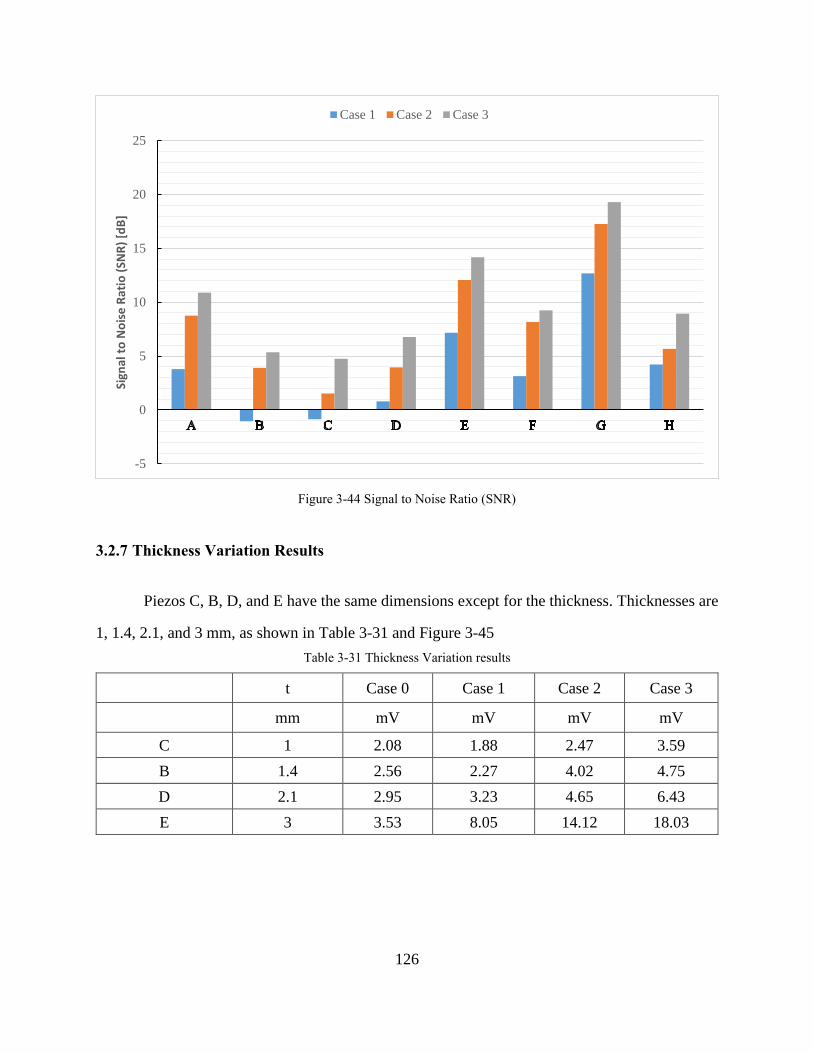
126
3.2.7 Thickness Variation Results
Piezos C, B, D, and E have the same dimensions except for the thickness. Thicknesses are
1, 1.4, 2.1, and 3 mm, as shown in Table 3-31 and Figure 3-45
Table 3-31 Thickness Variation results
t Case 0 Case 1 Case 2 Case 3
mm mV mV mV mV
C 1 2.08 1.88 2.47 3.59
B 1.4 2.56 2.27 4.02 4.75
D 2.1 2.95 3.23 4.65 6.43
E 3 3.53 8.05 14.12 18.03
-5
0
5
10
15
20
25
Sign
al t
o N
ois
e R
atio
(SN
R)
[dB
]Case 1 Case 2 Case 3
Figure 3-44 Signal to Noise Ratio (SNR)

127
As mentioned before, the voltage is increased when the flow increased for each piezo. Also,
the voltage output increased when the thickness is increased. Piezo-E with a thickness of 3mm and
the rest of the dimensions are the same as other cases. Therefore, the drag force and velocities are
the same. Therefore, increasing the thickness case increasing in voltage output. The maximum
voltage generated is 18 mV in Piezo-E at Case-3, and it is 5 times greater than Case 0. At the same
time, Case 0 in all piezos has the relatively same value.
0
2
4
6
8
10
12
14
16
18
20
1 1.4 2.1 3
Vo
lta
ge
ou
tpu
t [m
V]
Tickness (t) [mm]
Case 0 Case 1 Case 2 Case 3
Figure 3-45 Thickness variation voltage output

128
3.2.8 Area to Thickness Variation Results
Piezo A and B have a thickness of 1.5 and 1.4 mm. The aspect ratio is 1.5 and 1.3, and their
areas are 140 and 300 mm2. The area to thickness ratios is 93 and 214, and the corresponding
voltage output is represented in Table 3-32.
Table 3-32 Piezo sensors with the area to thickness variation
A/t Case 0 Case 1 Case 2 Case 3
mm2/mm mV mV mV mV
A 93 0.99 1.53 2.71 3.46
B 214 2.56 2.27 4.02 4.75
Figure 3-46 shows the voltage output results, and it shows that the voltage increases with
the flow. The differences between the two ratios are almost double, but the voltage output
differences are not significant (about 20%). More cases needed to be evaluated to confirm if the
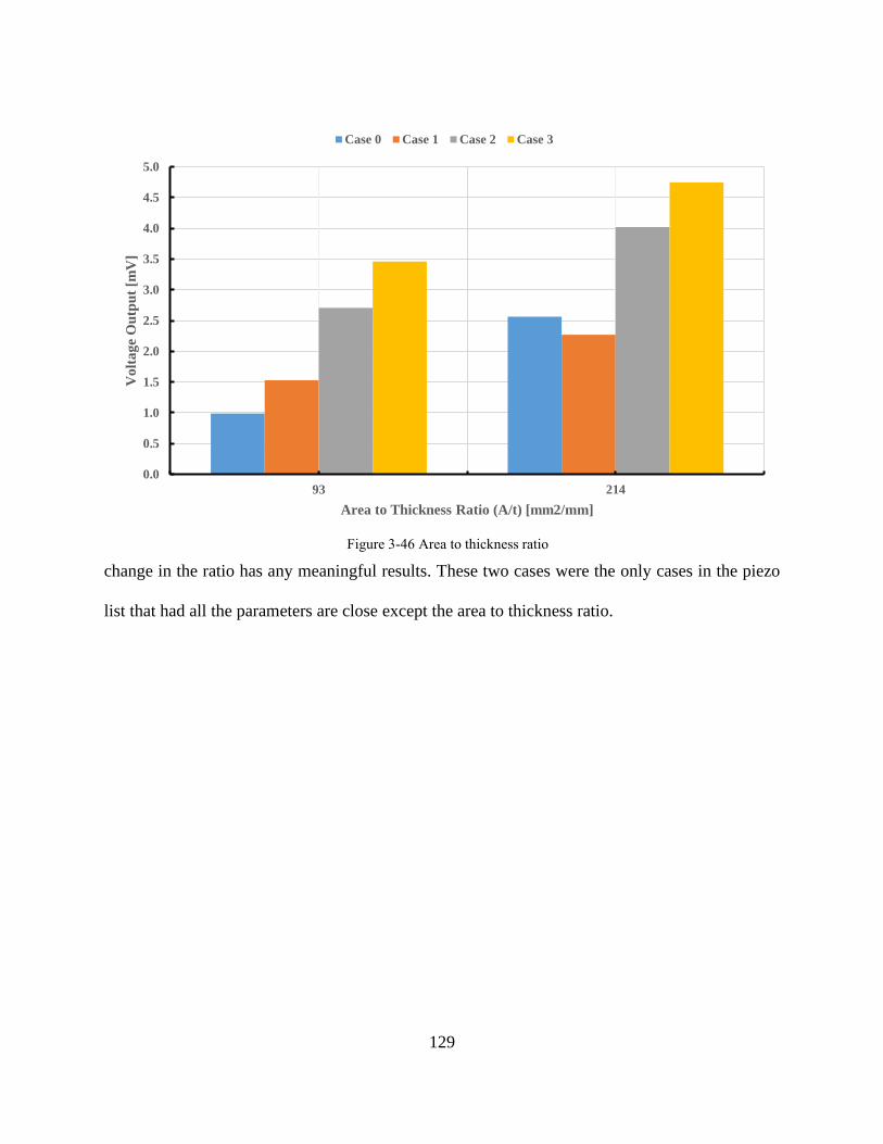
129
change in the ratio has any meaningful results. These two cases were the only cases in the piezo
list that had all the parameters are close except the area to thickness ratio.
0.0
0.5
1.0
1.5
2.0
2.5
3.0
3.5
4.0
4.5
5.0
93 214
Vo
lta
ge
Ou
tpu
t [m
V]
Area to Thickness Ratio (A/t) [mm2/mm]
Case 0 Case 1 Case 2 Case 3
Figure 3-46 Area to thickness ratio
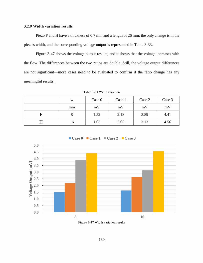
130
3.2.9 Width variation results
Piezo F and H have a thickness of 0.7 mm and a length of 26 mm; the only change is in the
piezo's width, and the corresponding voltage output is represented in Table 3-33.
Figure 3-47 shows the voltage output results, and it shows that the voltage increases with
the flow. The differences between the two ratios are double. Still, the voltage output differences
are not significant—more cases need to be evaluated to confirm if the ratio change has any
meaningful results.
Table 3-33 Width variation
w Case 0 Case 1 Case 2 Case 3
mm mV mV mV mV
F 8 1.52 2.18 3.89 4.41
H 16 1.63 2.65 3.13 4.56
0.0
0.5
1.0
1.5
2.0
2.5
3.0
3.5
4.0
4.5
5.0
8 16
Volt
age
Ou
tpu
t [m
V]
Width [mm]
Case 0 Case 1 Case 2 Case 3
Figure 3-47 Width variation results

131
3.2.10 Aspect Ratio Variation
Piezo D and G have a thickness of 2.1 mm and an area of 300 mm2. The only change is in
the aspect ratio of the piezo and corresponding voltage output represented in Table 3-34
Figure 3-47 shows the voltage output results, and it shows that the voltage increases with
the flow. The differences between the two ratios are double. Still, the voltage output differences
are not significant—more cases need to be evaluated to confirm if the ratio change has any
meaningful results.
Table 3-34 Piezo sensors with aspect ratio variation
l/w Case 0 Case 1 Case 2 Case 3
mm mV mV mV mV
D 1.3 2.95 3.23 4.65 6.43
G 12 3.27 14.08 23.84 30.11
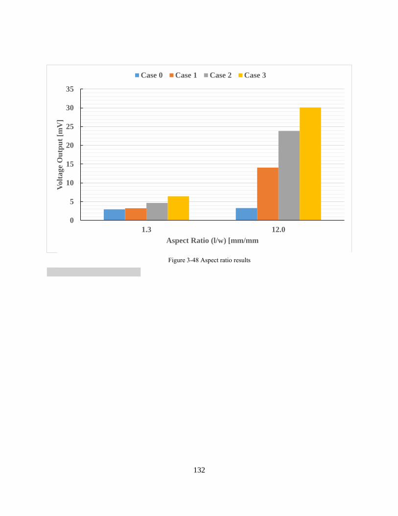
132
0
5
10
15
20
25
30
35
1.3 12.0
Volt
age
Ou
tpu
t [m
V]
Aspect Ratio (l/w) [mm/mm
Case 0 Case 1 Case 2 Case 3
Figure 3-48 Aspect ratio results

133
3.2.11 Piezo Empirical Equation
As mentioned in the theory and test matrix sections, The multi-linear regression equation
is
𝑌 = 𝛽0 +∑𝛽𝑖𝑋𝑖
𝑛
𝑖=1
+ 𝜖 3.2
The empirical voltage output equation
𝑉 = 𝑎. (
𝑙
𝑤)𝑏
. (𝐴
𝑡)𝑐
. 𝑣𝑑 3.3
After the log transformation on these values, the data plugged in SigmaPlot software, and
multi-linear regression analysis were performed to calculate the equation 2.12. 1
𝐿𝑜𝑔10(𝑉) = 𝐿𝑜𝑔10(𝑎) + 𝑏 𝐿𝑜𝑔10 (
𝑙
𝑤) + 𝑐 𝐿𝑜𝑔10 (
𝐴
𝑡) + 𝑑 𝐿𝑜𝑔10(𝑣) 3.4
The dependent variable for the multi-linear regression analysis is the 𝐿𝑜𝑔10(𝑉), and the
independent variables are 𝐿𝑜𝑔10(𝑣), 𝐿𝑜𝑔10 (𝑙
𝑤) , 𝑎𝑛𝑑 𝐿𝑜𝑔10 (
𝐴
𝑡). Where the voltage (𝑉) is
recorded from the experiment, the velocity (𝑣) calculated from the flow rate (measured in the
experiment), where the manufacturer provided the value of the aspect ratio (𝑙
𝑤) and the area to
thickness ratio (𝐴
𝑡). In total, one dependent and three independent variables, with 96 data points
from all the analysis experiments.
1 The full report is provided in the appendix

134
3.2.11.1 SigmaPlot Report
From the sigmaplot report
𝑅 𝑅2 𝑅𝑎𝑑𝑗2
0.767 0.588 0.575
Where 𝑅, the correlation coefficient, and 𝑅2, the coefficient of determination is both
measures of how well the regression model describes the data. 𝑅 values near 1 indicate that the
straight line is a good description of the relation between the independent and dependent variables.
𝑅𝑎𝑑𝑗2 It is also a measure of how well the regression model describes the data but considers
the number of independent variables, reflecting the degrees of freedom. Larger values (nearer to
1) indicate that the equation is a good description of the relation between the independent and
dependent variables. The results are acceptable, with room for improvement with more data points
in future work.
The standard error of the estimate, syx, is 0.23, and it is a measure of the actual variability
about the regression line of the underlying population. The underlying population generally falls
within about two standard errors of the observed sample.
The statistically summary table:
Coefficient Std. Error t P
𝛽0 -3.147 0.0932 -33.778 <0.001
𝛽1 0.488 0.0996 4.894 <0.001
𝛽2 -0.479 0.0914 -5.249 <0.001
𝛽3 0.637 0.0742 8.591 <0.001
Where

135
• Coefficients. The value for the constant (intercept or 𝛽0) and the coefficient of the
independent variable (slope or 𝛽1, 𝛽2, 𝛽3) for the regression model are listed.
• Standard Error. The intercept and slope's standard errors measure the precision of
the regression coefficients' estimates (analogous to the standard error of the mean).
The actual regression coefficients of the underlying population generally fall within
about two standard errors of the observed sample coefficients. These values are
used to compute t and confidence intervals for the regression.
• t Statistic. The t statistic tests the null hypothesis that the independent variable's
coefficient is zero; that is, the independent variable does not contribute to predicting
the dependent variable. t is the ratio of the regression coefficient to its standard
error, or
𝑡 =𝑟𝑒𝑔𝑟𝑒𝑠𝑠𝑖𝑜𝑛 𝑐𝑜𝑒𝑓𝑓𝑖𝑐𝑖𝑒𝑛𝑡
𝑠𝑡𝑎𝑛𝑑𝑒𝑟 𝑒𝑟𝑟𝑜𝑟 𝑜𝑓 𝑟𝑒𝑔𝑟𝑒𝑠𝑠𝑖𝑜𝑛 𝑐𝑜𝑒𝑓𝑓𝑖𝑒𝑛𝑡
The "large" t values conclude that the independent variable and can be used to
predict the dependent variable
• P-Value. P is the P-value calculated for t. The P-value is the probability of being
wrong in concluding a real association between the variables. The smaller the P-
value, the greater the probability that the independent variable can predict the
dependent variable. Traditionally, the independent variable can be used to predict
the dependent variable when P < 0.05.

136
The analysis of variance:
DF SS MS F P
Regression 3 6.929 2.310 43.830 <0.001
Residual 92 4.848 0.0527
Total 95 11.776 0.124
Where
• DF (Degrees of Freedom) represent the number of observations and variables in the
regression equation.
o The regression degrees of freedom is a measure of the number of
independent variables in the regression equation
o The residual degrees of freedom is a measure of the number of observations
less the number of terms in the equation
o The total degrees of freedom is a measure of total observations
• SS (Sum of Squares). The sum of squares are measures of variability of the
dependent variable.
o The sum of squares due to regression (𝑆𝑆𝑟𝑒𝑔 ) measures the difference of
the regression line from the mean of the dependent variable
o The residual sum of squares (𝑆𝑆𝑟𝑒𝑠 ) is a measure of the residuals' size,
which are the differences between the dependent variable's observed values
and the values predicted by the regression model.
o The total sum of squares (𝑆𝑆𝑡𝑜𝑡 ) is a measure of the overall variability of
the dependent variable about its mean value

137
• MS (Mean Square). The mean square provides two estimates of the population
variances. Comparing these variance estimates is the basis of the analysis of
variance.
The mean square regression is a measure of regression variation from the mean of
the dependent variable, or
𝑆𝑆𝑟𝑒𝑔
𝐷𝐹𝑟𝑒𝑔= 𝑀𝑆𝑟𝑒𝑔
• The residual mean square is a measure of the variation of the residuals about the
regression line, or
𝑆𝑆𝑟𝑒𝑠𝐷𝐹𝑟𝑒𝑠
= 𝑀𝑆𝑟𝑒𝑠
• F Statistic is a gauge of the contribution of the independent variable in predicting
the dependent variable. It is the ratio
𝑀𝑆𝑟𝑒𝑔
𝑀𝑆𝑟𝑒𝑠= 𝐹
If F is a large number, the independent variable contributes to the prediction of the
dependent variable. If the F ratio is around one, conclude that there is no association
between the variables
3.2.11.2 Empirical Equation Model
After plugging the coefficient from the report above, the regression model can be written
as
𝑉 = 7.13 × 10⁻⁴. 𝑣0.488. (
𝐴
𝑡)−0.479
. (𝑙
𝑤)0.637
3.5

138
From the equation above, the dominant variable in this equation is the aspect ratio (𝑙
𝑤) It
has a power of 0.637. According to the width variation results, the width does not have a major
impact on the signal. Therefore, most likely that length has a main effect on the signal output. The
velocity is the second dominant variable with a power of 0.49, which is very different from
equation 2.4, where the velocity has the power of 2. In that equation, the force is assumed to be
applied as a statistic force where the force applied in the experiment is dynamic as the output signal
is oscillating. The output signal has been transferred using the root mean square method to use the
signal's power as a useful signal. The dynamic force and the RMS value from equation 3.5,
resulting in velocity to be a function of power 0.49 (almost square root of velocity). More tests are
required to validate this assumption. Finally, the area to thickness ratio has a power of -0.479,
which means that the thickness is probational, and the area is inversely proportional to the signal
output.
To visuals the goodness of the model, the actual value collected from the experiment and
the data was predicted using the model of multi-linear regression were plotted ageist each other
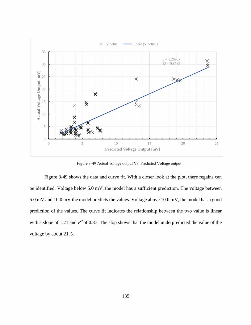
139
Figure 3-49 shows the data and curve fit. With a closer look at the plot, there regains can
be identified. Voltage below 5.0 mV, the model has a sufficient prediction. The voltage between
5.0 mV and 10.0 mV the model predicts the values. Voltage above 10.0 mV, the model has a good
prediction of the values. The curve fit indicates the relationship between the two value is linear
with a slope of 1.21 and 𝑅2of 0.87. The slop shows that the model underpredicted the value of the
voltage by about 21%.
y = 1.2098x
R² = 0.8785
0
5
10
15
20
25
30
35
0 5 10 15 20 25
Act
ua
l V
olt
ag
e O
utp
ut
[mV
]
Predicted Voltage Output [mV]
V actual Linear (V actual)
Figure 3-49 Actual voltage output Vs. Predicted Voltage output
140
Chapter 4: Summary and Conclusions
4.1 Summary of the Results
In many literature applications, the piezoelectric effect produces a voltage that is captured
for energy harvesting applications. However, in this study, the voltage output is used for a different
purpose. A piezoelectric cantilever beam is placed in a flowing air stream and used to measure a
fluid's velocity. The piezoelectric is advantageous due to its potential durability at higher
temperatures and self-powered characteristics. This study has two phases to address the velocity
profile influence on the output voltage and the piezoelectric sensor's geometry effect.
Phase I has two different experimental setups with rectangular and circular cross-sections
to test the velocity profile's impact. The following summarizes the main findings from this study:
• The voltage increases non-linearly as the velocity is increased in the test sections of the
experimental setups for both piezoelectrics, which indicates that the piezoelectric voltage
output could be calibrated to correspond to different flow velocities.
• Due to the different cross-section setup, the corresponding velocity profiles produced
different voltage outputs even with the same amount of drag force applied on the sensor.
The slop on RTS is estimated to be 1.9 times higher than the slop on CTS.
• The maximum voltage output in RTS at the maximum effective velocity is 258.2 mV,
where it is 135.3 mV in CTS.
• The relationship between drag force/velocity and voltage produced by the sensor is
observed to be linear, indicating that this could be calibrated as a sensor
141
Phase II used eight piezoelectric specimens with the same cross-sectional area. These
piezoelectrics had varying thickness, width, and length to test geometry's effect on the sensor’s
voltage output. The following summarizes the main findings from this portion of the study:
• The Chemical Looping Reactor system at the National Energy Technology
Laboratory provided airflow to pass to the GTS experimental system. Four cases
were tested 0, 2.24, 4.85, and 7.56 m/s.
• Based on Phase I's findings, the voltage output was determined primarily depending
on the thickness of the piezoelectric, the velocity of the flow, aspect ratio, and area
to thickness ratio of the piezoelectric.
• A multi-linear regression analysis was used to determine the relationship between
the voltage and the other important factors. The following is the best-fit curve
equation that may be used to predict the sensor's voltage output. The equation has
an R2 value of 57%.
• This equation shows that although it was expected that velocity varies to the square,
velocity varies to the 0.488 power. Thus, the effect of drag force on the sensor is
not the only force, and there may be multiple factors influencing the effect of
velocity on the sensor. The other factors may include pressure distributions within
the system, material effects, and the sensor's oscillating behavior, resulting in a
variation to the square-root of the velocity.
𝑉 = 7.13 × 10⁻⁴. 𝑣0.488. (
𝐴
𝑡)−0.479
. (𝑙
𝑤)0.637

142
4.2 Conclusion
Based on the results found in this dissertation, the piezoelectric materials presented here
may be used as a flow sensor. The design tested in this study was a cantilever beam interacting
with the flow. The main factors that determined the voltage output in the order of importance were
aspect ratio, velocity, and thickness to area ratio. It is thought that dynamic loads applied to the
beam caused voltage variation with velocity to vary with a power of 0.5 instead of the original
squared power. The model had an error of 13% based on regression analysis and curve fit.
4.3 Future Work
The experiments performed in this study used essentially the same geometry and, thus, the
same drag coefficient, fluid density, and piezoelectric coefficient. the other variables could be
varied to check their impact on the signal output and develop a more inclusive equation. Therefore,
tests with a piezoelectric beam or other cross-section shapes such as circular, triangular could be
used. Furthermore, the variation of the piezoelectric coefficient with temperature may also be done
to determine the voltage signal's effect.
Another important factor that should be investigated is the lifetime of the sensing element.
Therefore, a fatigue analysis is needed to estimate the lifetime of the sensor. Also, the degradation
of the piezoelectric coefficient with time is needed to be estimated as well to evaluate how long
the sensor will provide an accurate signal without recalibration

143
References
[1] “U.S. energy facts explained - consumption and production - U.S. Energy Information
Administration (EIA).” [Online]. Available: https://www.eia.gov/energyexplained/us-
energy-facts/. [Accessed: 24-Sep-2020].
[2] A. Del Rosario, “Comparison of Energy Systems Using Life Cycle Assessment Officers of
the World Energy Council,” 2004.
[3] US Department of Energy, “Frequently Asked Questions (FAQs) - U.S. Energy Information
Administration (EIA),” EIA, 2019. [Online]. Available:
https://www.eia.gov/tools/faqs/faq.php?id=77&t=11. [Accessed: 09-Oct-2020].
[4] K. Uchino and T. Ishii, “Energy flow analysis in piezoelectric energy harvesting systems,”
Ferroelectrics, vol. 400, no. 1, pp. 305–320, 2010.
[5] H. W. Kim et al., “Energy harvesting using a piezoelectric ‘cymbal’ transducer in dynamic
environment,” Japanese J. Appl. Physics, Part 1 Regul. Pap. Short Notes Rev. Pap., vol.
43, no. 9 A, pp. 6178–6183, 2004.
[6] B. Li, J. H. You, and Y. J. Kim, “Low frequency acoustic energy harvesting using PZT
piezoelectric plates in a straight tube resonator,” Smart Mater. Struct., vol. 22, no. 5, 2013.
[7] R. Carter and R. Kensley, Introduction to Piezoelectric Transducers, vol. 53, no. 9. 2020.
[8] P. Paufler, “Fundamentals of Piezoelectricity,” Zeitschrift für Krist., vol. 199, no. 1–2, pp.
158–158, 1992.
[9] B. Han, X. Yu, and J. Ou, “Challenges of Self-Sensing Concrete,” Self-Sensing Concr.
Smart Struct., pp. 361–376, 2014.
[10] I. Baker and I. Baker, “Lead Zirconate Titanate,” in Fifty Materials That Make the World,
2018, pp. 111–115.

144
[11] APC International, “PZT Properties & PZT Manufacturing,” americanpizeo.com, 2016.
[Online]. Available: https://www.americanpiezo.com/piezo-theory/pzt.html. [Accessed:
15-Oct-2020].
[12] U. Guler, M. S. E. Sendi, and M. Ghovanloo, “A dual-mode passive rectifier for wide-range
input power flow,” in Midwest Symposium on Circuits and Systems, 2017, vol. 2017-
August, pp. 1376–1379.
[13] R. Ambrosio, A. Jimenez, J. Mireles, M. Moreno, K. Monfil, and H. Heredia, “Study of
piezoelectric energy harvesting system based on PZT,” in Integrated Ferroelectrics, 2011,
vol. 126, no. 1, pp. 77–86.
[14] A. Čeponis, D. Mažeika, G. Kulvietis, and Y. Yang, “Piezoelectric cantilevers for energy
harvesting with the irregular design of the cross-sections,” Mechanika, vol. 24, no. 2, pp.
221–231, 2018.
[15] W. J. Choi, Y. Jeon, J. H. Jeong, R. Sood, and S. G. Kim, “Energy harvesting MEMS device
based on thin-film piezoelectric cantilevers,” in Journal of Electroceramics, 2006, vol. 17,
no. 2–4, pp. 543–548.
[16] J. Sirohi and R. Mahadik, “Harvesting wind energy using a galloping piezoelectric beam,”
J. Vib. Acoust. Trans. ASME, vol. 134, no. 1, pp. 1–8, 2012.
[17] L. A. Weinstein, M. R. Cacan, P. M. So, and P. K. Wright, “Vortex shedding induced energy
harvesting from piezoelectric materials in heating, ventilation and air conditioning flows,”
Smart Mater. Struct., vol. 21, no. 4, 2012.
[18] D. Shen, J. H. Park, J. Ajitsaria, S. Y. Choe, H. C. Wikle, and D. J. Kim, “The design,
fabrication, and evaluation of a MEMS PZT cantilever with an integrated Si proof mass for
vibration energy harvesting,” J. Micromechanics Microengineering, vol. 18, no. 5, 2008.

145
[19] M. Rezaei, S. E. Khadem, and P. Firoozy, “Broadband and tunable PZT energy harvesting
utilizing local nonlinearity and tip mass effects,” Int. J. Eng. Sci., vol. 118, pp. 1–15, Sep.
2017.
[20] E. Abbott, A. Flannery, A. Microsystems, and D. Cagle, “WeES3-1 Control Issues for
MEMS,” Changes, pp. 3039–3047, 2005.
[21] G. Ciuti, L. Ricotti, A. Menciassi, and P. Dario, “MEMS sensor technologies for human-
centered applications in healthcare, physical activities, safety, and environmental sensing:
A review on research activities in Italy,” Sensors (Switzerland), vol. 15, no. 3, pp. 6441–
6468, Mar. 2015.
[22] J. H. K. Iv, B. C. Claus, and J. C. Kinsey, “A Navigation Solution Using a MEMS IMU,
Model-Based Dead-Reckoning, and One-Way-Travel-Time Acoustic Range Measurements
for Autonomous Underwater Vehicles,” IEEE J. Ocean. Eng., vol. 44, no. 3, pp. 664–682,
2019.
[23] S. Silvestri and E. Schena, “Micromachined Flow Sensors in Biomedical Applications,”
Micromachines, vol. 3, no. 2, pp. 225–243, Mar. 2012.
[24] O. Sazhin, “Liquid flow meter based on a thermal anemometer microsensor,” J. Appl. Fluid
Mech., vol. 9, no. 4, pp., 1991–1996, 2016.
[25] V. Balakrishnan, T. Dinh, H. P. Phan, D. V. Dao, and N. T. Nguyen, “Highly sensitive 3C-
SiC on glass-based thermal flow sensor realized using MEMS technology,” Sensors
Actuators, A Phys., vol. 279, pp. 293–305, Aug. 2018.
[26] A. G. P. Kottapalli, M. Asadnia, E. Kanhere, M. S. Triantafyllou, and J. M. Miao, “Smart
skin of self-powered hair cell flow sensors for sensing hydrodynamic flow phenomena,” in
2015 Transducers - 2015 18th International Conference on Solid-State Sensors, Actuators

146
and Microsystems, TRANSDUCERS 2015, 2015, pp. 387–390.
[27] C. Liu et al., “A micromachined flow shear-stress sensor based on thermal transfer
principles,” J. Microelectromechanical Syst., vol. 8, no. 1, pp. 90–98, Mar. 1999.
[28] M. Sheplak, V. Chandrasekaran, A. Cain, T. Nishida, L. N. Cattafesta III, and L. N.
Cattafesta, “Characterization of a Silicon-Micromachined Thermal Shear-Stress Sensor,”
AIAA J., vol. 40, no. 6, pp. 8–11, May 2002.
[29] N. Svedin, E. Stemme, and G. Stemme, “A static turbine flow meter with a micromachined
silicon torque sensor,” J. Microelectromechanical Syst., vol. 12, no. 6, pp. 937–946, Dec.
2003.
[30] N. Svedin, E. Kälvesten, E. Stemme, and G. Stemme, “A new silicon gas-flow sensor based
on lift force,” J. Microelectromechanical Syst., vol. 7, no. 3, pp. 303–308, Sep. 1998.
[31] T. Ebefors, E. Kalvesten, and G. Stemme, “Three-dimensional silicon triple-hot-wire
anemometer based on polyimide joints,” in Proceedings of the IEEE Micro Electro
Mechanical Systems (MEMS), 1998, pp. 93–98.
[32] H. Liu, S. Zhang, R. Kathiresan, T. Kobayashi, and C. Lee, “Development of piezoelectric
microcantilever flow sensor with wind-driven energy harvesting capability,” Appl. Phys.
Lett., vol. 100, no. 22, pp. 2010–2013, 2012.
[33] Y. H. Seo and B. H. Kim, “A self-resonant microflow velocity sensor based on a resonant
frequency shift by flow-induced vibration,” J. Micromechanics Microengineering, vol. 20,
no. 7, 2010.
[34] Y. H. Wang, C. Y. Lee, and C. M. Chiang, “A MEMS-based air flow sensor with a free-
standing microcantilever structure,” Sensors, vol. 7, no. 10, pp. 2389–2401, 2007.
[35] Q. Li, J. Xing, D. Shang, and Y. Wang, “A flow velocity measurement method based on a

147
PVDF piezoelectric sensor,” Sensors (Switzerland), vol. 19, no. 7, 2019.
[36] M. Asadnia, A. G. P. Kottapalli, J. Miao, M. E. Warkiani, and M. S. Triantafyllou,
“Artificial fish skin of self-powered micro-electromechanical systems hair cells for sensing
hydrodynamic flow phenomena,” J. R. Soc. Interface, vol. 12, no. 111, 2015.
[37] C. Ghouila-Houri et al., “High-temperature gradient calorimetric wall shear stress micro-
sensor for flow separation detection,” Sensors Actuators, A Phys., vol. 266, pp. 232–241,
Oct. 2017.
[38] I. Etchart et al., “MEMS sensors for density-viscosity sensing in a low-flow microfluidic
environment,” Sensors Actuators, A Phys., vol. 141, no. 2, pp. 266–275, Feb. 2008.
[39] F. Ejeian et al., “Design and applications of MEMS flow sensors: A review,” Sensors
Actuators, A Phys., vol. 295, pp. 483–502, Aug. 2019.
[40] B. Tian, H. F. Li, H. Yang, D. L. Song, X. W. Bai, and Y. L. Zhao, “A MEMS SOI-based
piezoresistive fluid flow sensor,” Rev. Sci. Instrum., vol. 89, no. 2, p. 025001, Feb. 2018.
[41] B. Abbasnejad, W. Thorby, A. Razmjou, D. Jin, M. Asadnia, and M. Ebrahimi Warkiani,
“MEMS piezoresistive flow sensors for sleep apnea therapy,” Sensors Actuators, A Phys.,
vol. 279, pp. 577–585, Aug. 2018.
[42] J. J. Kuchle and N. D. Love, “Self-powered wireless thermoelectric sensors,” Meas. J. Int.
Meas. Confed., vol. 47, no. 1, pp. 26–32, 2014.
[43] M. R. H. Sarker, J. L. Silva, M. Castañeda, B. Wilburn, Y. Lin, and N. Love,
“Characterization of the pyroelectric coefficient of a high-temperature sensor,” J. Intell.
Mater. Syst. Struct., vol. 29, no. 5, pp. 938–943, 2018.
[44] J. Hjelmgren and Jan Hjelmgren, Dynamic Measurement of Pressure - A Literature Survey.
2002.

148
[45] A. A. Barlian, W. T. Park, J. R. Mallon, A. J. Rastegar, and B. L. Pruitt, “Review:
Semiconductor piezoresistance for microsystems,” Proc. IEEE, vol. 97, no. 3, pp. 513–552,
2009.
[46] S. Li, J. Yuan, and H. Lipson, “Ambient wind energy harvesting using cross-flow
fluttering,” J. Appl. Phys., vol. 109, no. 2, 2011.
[47] H. Li, C. Tian, and Z. D. Deng, “Energy harvesting from low-frequency applications using
piezoelectric materials,” Applied Physics Reviews, vol. 1, no. 4. 2014.
[48] H. J. Lee, S. Sherrit, L. P. Tosi, P. Walkemeyer, and T. Colonius, “Piezoelectric energy
harvesting in internal fluid flow,” Sensors (Switzerland), vol. 15, no. 10, pp. 26039–26062,
2015.
[49] A. Čeponis, D. Mažeika, and V. Bakanauskas, “Trapezoidal Cantilevers with Irregular
Cross-Sections for Energy Harvesting Systems,” Appl. Sci., vol. 7, no. 2, p. 134, 2017.
[50] H. S. Kim, J. H. Kim, and J. Kim, “A review of piezoelectric energy harvesting based on
vibration,” Int. J. Precis. Eng. Manuf., vol. 12, no. 6, pp. 1129–1141, 2011.
[51] C. Xie, B. Oelmann, and G. Thungström, “Finite Element Analysis of PZT-based Air Flow
Sensor Independent degree project - second cycle,” no. December 2017.
[52] R. J. Mckee, S. P. Siebenaler, and D. M. Deffenbaugh, “Increased flexibility of turbo-
Compressors in natural gas transmission through direct surge control,” 2003.
[53] D. A. Fink, N. A. Cumpsty, and E. M. Greitzer, “Surge dynamics in a free-spool centrifugal
compressor system,” in Proceedings of the ASME Turbo Expo, 1991, vol. 1.
[54] H. Shen, C. Zhang, J. Zhang, B. Yang, and B. Jia, “Applicable and comparative research of
compressor mass flow rate and isentropic efficiency empirical models to a large-scale
marine compressor,” Energies, vol. 13, no. 1, 2019.

149
[55] A. Hafaifa, B. Rachid, and G. Mouloud, “Modelling of surge phenomena in a centrifugal
compressor: Experimental analysis for control,” Syst. Sci. Control Eng., vol. 2, no. 1, pp.
632–641, Dec. 2014.
[56] I. J. Day, “Axial compressor performance during the surge,” J. Propuls. Power, vol. 10, no.
3, pp. 329–336, 1994.
[57] C. S. Tan, I. Day, S. Morris, and A. Wadia, “Spike-type compressor stall inception,
detection, and control,” Annu. Rev. Fluid Mech., vol. 42, pp. 275–300, Jan. 2010.
[58] E. Sundström, B. Semlitsch, and M. Mihăescu, “Generation Mechanisms of Rotating Stall
and Surge in Centrifugal Compressors,” Flow, Turbul. Combust., vol. 100, no. 3, pp. 705–
719, Apr. 2018.
[59] E. M. Greitzer, “Surge and rotating stall in axial flow compressors: Part II: Theoretical
compression system model,” J. Eng. Gas Turbines Power, vol. 98, no. 2, pp. 190–198, Apr.
1976.
[60] E. M. Greitzer, “Surge and rotating stall in axial flow compressors,” J. Eng. Gas Turbines
Power, vol. 98, no. 2, pp. 199–211, Apr. 1976.
[61] I. Shahin, M. Gadala, M. Alqaradawi, and O. Badr, “Large-eddy simulation for a deep surge
cycle in a high-speed centrifugal compressor with a vaned diffuser,” J. Turbomach., vol.
137, no. 10, Oct. 2015.
[62] B. Semlitsch and M. Mihăescu, “Flow phenomena were leading to a surge in a centrifugal
compressor,” Energy, vol. 103, pp. 572–587, May 2016.
[63] T. Benson, K. Gemba, and T. Benson, “Shape Effects on Drag,” Dep. Aerosp. Eng. Calif.
State Univ. Long Beach, Calif., vol. 90840, no. May 2007, pp. 2–5, 2010.
[64] E. Buckingham, “On physically similar systems; illustrations of the use of dimensional

150
equations,” Phys. Rev., vol. 4, no. 4, pp. 345–376, 1914.
[65] A. Tsai, P. Pezzini, D. Tucker, and K. M. Bryden, “Multiple-model adaptive control of a
hybrid solid oxide fuel cell gas turbine power plant simulator,” J. Electrochem. Energy
Convers. Storage, vol. 16, no. 3, 2019.
[66] V. Zaccaria, D. Tucker, and A. Traverso, “Cold-Air Bypass Characterization for Thermal
Management of Fuel Cell Gas Turbine Hybrids,” J. Eng. Gas Turbines Power, vol. 139, no.
6, p. 062701, 2017.
[67] D. N. E. T. L. / D. of E. Tucker, N. D. Love, and Y. Lin, “Cooperative Research and
Development Agreement (CRADA) Statement of Work (SOW) The University of Texas El
Paso and NETL Principal Investigators National Energy Technology Laboratory (NETL),”
El Paso, TX, 2018.
[68] Y. Lin and N. Love, “Systems and methods for wireless temperature sensing,” 2017.
[69] M. R. H. Sarker, H. Karim, R. Martinez, N. Love, and Y. Lin, “A Lithium Niobate High-
Temperature Sensor for Energy System Applications,” IEEE Sens. J., vol. 16, no. 15, pp.
5883–5888, Aug. 2016.
[70] NETL’s Multiphase Flow Science, “Chemical Looping Combustion - Multiphase Flow
Science Group at NETL.” [Online]. Available: https://mfix.netl.doe.gov/research/chemical-
looping-combustion/. [Accessed: 19-Oct-2020].
[71] G. Zambonini, “Unsteady dynamics of corner separation in a linear compressor cascade,”
2016.
[72] QuickerSim CFD Toolbox for MATLAB, “Tutorial 23 – Inlet Velocity Profiles in Channel
Flows,” 2017. [Online]. Available: https://quickersim.com/tutorial/tutorial-23-inlet-
velocity-profiles-channel-flows/. [Accessed: 11-Nov-2020].

151
Appendix
Appendix A
Test Procedure
Setup connectivity
Ensure the physical configuration follows the diagram (System fluid schematic). First of
all, connect all equipment following the test procedure instructions and then set parameters before
testing. Also, follow the safety rules that describe the use of Safety glasses inside the lab and gloves
for manipulating the sensor
Following the Schematic diagram in chapter two, a 4-WIRE fan has power, ground, tach
signal, and a PWM input. The red wire (power) will be directly connected to the red port on the
power supplier and the blue wire (ground) to the power supplier's black port. All three devices are
connected to the ground and connected to the fan's negative wire connected to the power supplier's
black output, as showed. The power supplier used an Alligator Clip and Stacking Banana Plug for
both ports. Fan’s positive wire is connected directly to the positive output from the power supplier
PWM wire connected to the function generator output to control the duty cycles using a Test Lead
BNC Male to Test Clips wire. In this case, the Tachometer wire is connected to the first channel
on the oscilloscope using the Scope Clip Oscilloscope Probe cable. Two cable wires (positive and
negative wires) are connected to the piezoelectric ceramic, carefully making sure they are correctly
connected and not touching each other. Then they are connected to the corresponding Oscilloscope
channel to captured data. Cables used were a cable BNC Male to BNC Male cable and a BNC
Male cable to Test Clips wire. The piezoelectric fan, which has cables attached to it, just connected
the corresponding wires to the sensor and inserted it into the channel to process data.

152
Looking for the velocity profile, the anemometer and hotwire are portable devices and does
not require any connections. They are being placed at the same spot as the sensing element for
velocity measurements.
Instrumentation
1) Function generator
A function generator is set to a square wave function. Six blue buttons allow selecting the
output waveform parameters to control the fan’s duty cycles. The parameter value can be adjusted
with the numbered keys, arrow buttons, and the knob located in the front panel's upper-right corner
after selecting a parameter. The highlighted label corresponds to the parameter that is currently
selected, and its value will be shown on display. Adjust the Freq, Amplitude, Offset, Width, and
Duty Cycle parameters.
Table 0-1 Function generator parameters
Parameters Value Units
Frequency 2 kHz
Amplitude 2.5 V
Offset 1.25 V
High level 2.5 V
Low level 0 V
Amplitude and Offset softkeys toggle together to Hi-Level and Lo-Level, respectively.
Output button turns on the output voltage, which should be off to have a 100% duty cycle
2) Power supply
Power supplier is set to a nominal voltage of 24 V

153
3) DC Axial fan
After the fan turn on, it must be warmed up for 5 min to reach a steady-state
4) Oscilloscope configuration
A storage oscilloscope can capture a single event and display it continuously,
so the user can observe events that would otherwise appear too briefly to see directly
• To operate an oscilloscope, first, plug the electrical signal would like to view into one of
the oscilloscope’s inputs (channel one)
• Digital Oscilloscope is set to auto to display automatic calculations for the most efficient
display adjustment (changes will be made for different purposes)
• Click back on the menu to close Auto settings
• Click on CH1 (channel one) and set Coupling to DC, Bandwidth limit to “ON” status,
Probe x1 and digital filter must be off
• The vertical deflection is set to 100 mV
• The horizontal sweep is set to 10 seconds
• An oscilloscope's trigger function is essential to achieve precise signal characterization,
as it synchronizes the horizontal sweep of the oscilloscope to the appropriate point of the
signal. The trigger will be adjusted to stabilize repetitive waveforms as well as capture a
single-shot waveform. The trigger is set to the 50% button, which sets the trigger level to
the center of the signal
• Under standard menu bottoms, click on Acquire and make sure that Acquisition is set to
normal, sampling is on real-time, memory depth is set to long memory, and finally, sinx/x
is ‘ON.’

154
5) Testing
• During testing, all equipment should be on a table with no movement at all since it could
affect lectures on the oscilloscope
• After all, parameters are set and check, modified the necessary duty cycle for testing
• For multiple testing, 30 seconds is enough between each test to let the flow stabilize before
importing data
• A full duty cycle test consists on (20,30,40,50,60,70,80,100, and 20 %) and (2.5,5,10, and
15 m/s)
6) Post-test
• Connect a USB Flash Drive to the USB host of the oscilloscope
• Press the “Storage” button, and a menu appears on the right side of the screen
• Press the “Storage” button to select “Bit map” or ‘’ CSV’’. These files can be saved and
opened directly in Excel or other PC-based analysis tools.
• Data depth should be on maximum and Para Save set ‘ON’ to save the current oscilloscope
settings in a different format with the same file name
• Press the “External” button, and a new menu appears on the screen.
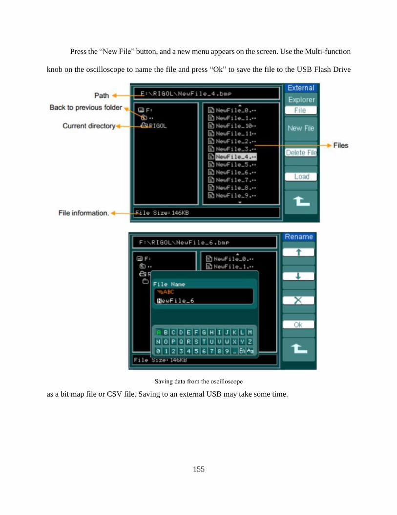
155
Press the “New File” button, and a new menu appears on the screen. Use the Multi-function
knob on the oscilloscope to name the file and press “Ok” to save the file to the USB Flash Drive
as a bit map file or CSV file. Saving to an external USB may take some time.
Saving data from the oscilloscope

156
Appendix B
Safety Considerations
Personal protective equipment (PPE) will be used at all times and for the following phases
of the experiments: Test Setup Buildup, Hardware Installation, and general test operations.
Personal Protective Equipment
Eyes Safety glasses shall be worn at all times when inside the lab
Feet Closed-toe shoes (steel toe) shall be worn at all times when inside the lab
Body Lab coats shall be worn at all times inside the lab
Ears Ear protection shall be worn by technicians inside the bunker when a loud noise is
occurred at the lab (above 15 dB)
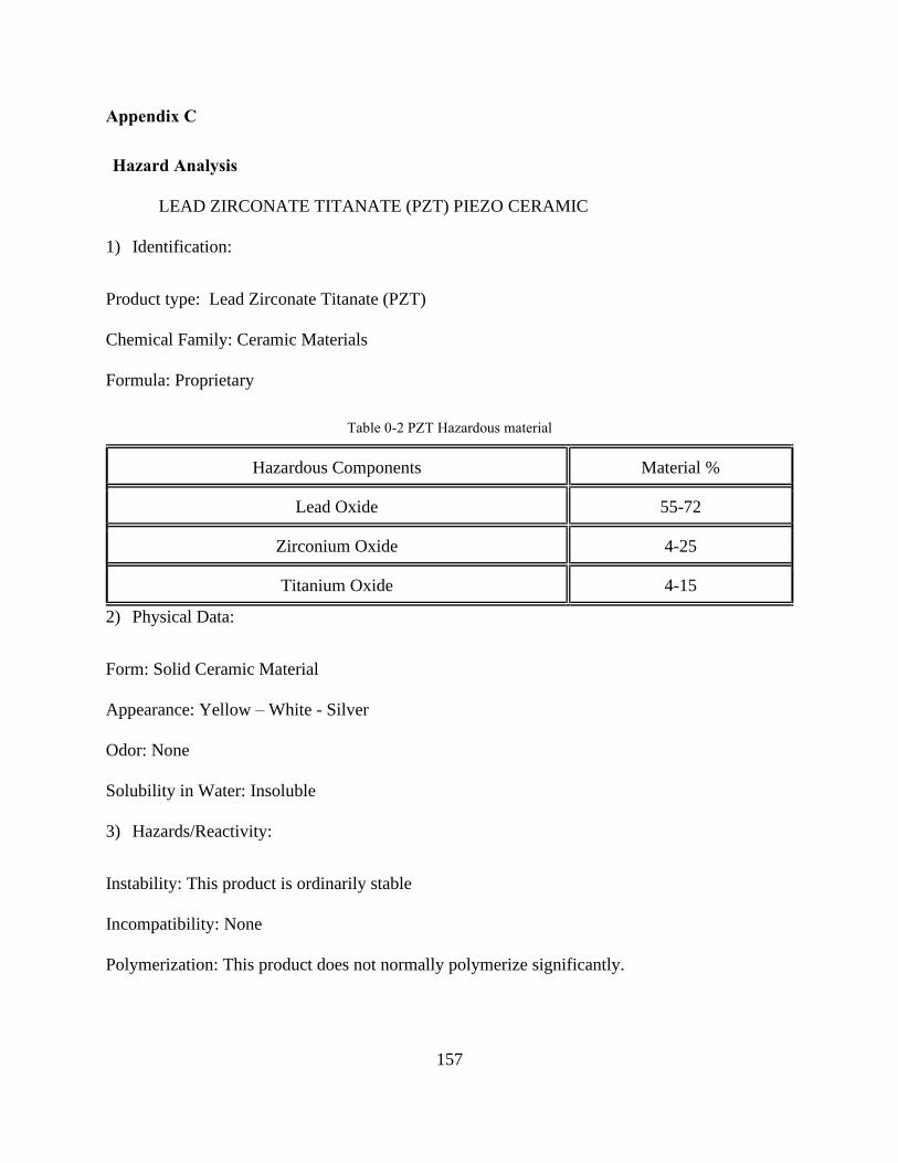
157
Appendix C
Hazard Analysis
LEAD ZIRCONATE TITANATE (PZT) PIEZO CERAMIC
1) Identification:
Product type: Lead Zirconate Titanate (PZT)
Chemical Family: Ceramic Materials
Formula: Proprietary
Table 0-2 PZT Hazardous material
Hazardous Components Material %
Lead Oxide 55-72
Zirconium Oxide 4-25
Titanium Oxide 4-15
2) Physical Data:
Form: Solid Ceramic Material
Appearance: Yellow – White - Silver
Odor: None
Solubility in Water: Insoluble
3) Hazards/Reactivity:
Instability: This product is ordinarily stable
Incompatibility: None
Polymerization: This product does not normally polymerize significantly.

158
4) Fire & Explosion Data:
Flash Point: None; a solid material
Fire & Explosion Hazards: None, nonflammable
5) Health Hazard Information:
Solid Lead Zirconate Titanate (PZT) ceramic materials are generally non-hazardous, but
toxic dust may be generated by breaking it or machining processes. The primary route of entry is
either by inhalation or ingestion. This material can be in the form of a powder or solid. If inhaled
or ingested, the toxicology of lead predominates. These hazards include the potential for damage
to the kidneys, blood-forming organs, the reproductive system, and the nervous system. Ingestion
can cause vomiting, diarrhea, nausea, and abdominal pain. Inhalation may irritate the nose and
throat, cough, dyspnea, chest pains, fever, and chills. PZT ceramics contain Lead, which is a known
carcinogen.
6) Material Safety Data Sheet (MSDS)
Piezoceramic Material Acute lead poisoning can lead to acute encephalopathy, which may
rapidly develop into seizures, coma, and, eventually, death.
7) Exposure Limits:
Table 0-3 PZT exposure limits
Material Name OSHA PEL (mg/m3) ACGIH TLV (mg/m3)

159
Lead 0.05 0.05
Zirconium Oxide 5.0 5.0
Titanium Oxide 15.0 (Total dust) 10
8) First Aid Instructions:
Ingestion: If conscious, induce vomiting.
Inhalation: Remove to fresh air and if breathing is difficult, give oxygen.
Skin Contact: Wash thoroughly.
Eye Contact: Flush with plenty of water for 15 minutes.
In all cases, seek appropriate medical advice & treatment.
9) Personal Protection Information:
Respiratory Protection: Selection of a suitable respirator will depend on the contaminant(s)
properties and their actual or expected air concentration(s) versus applicable limits. Gloves: Gloves
should be used when the possibility of skin contact exists. A special glove and glove material's
suitability should be determined as part of an overall glove personal protection program.
Considerations should include chemical breakthrough time, permeation rate; abrasion, cut and
puncture resistance; and duration of contact, etc. Recommended glove material: Latex.
Other personal protection practices: Appropriate eye protection such as safety glasses
should be used where the possibility of eye contact exists. Protective outer clothing should be used
where the possibility of body contact exists. Contaminated work clothing should not be allowed
out of the workplace. Smoking or consuming food or beverages should be prohibited where the
material is handled or stored after handling this material, washing hands thoroughly before leaving
the work area.

160
Additional Engineering Controls: Local exhaust ventilation is recommended where
airborne dust or powder is generated. Work practices and training may be required depending on
the exposure level. Many of these points are discussed in the OSHA Respiratory Protection
Standard
(29 CFR 1910.134), the OSHA Hazard Communication Standard (29 CFR 1910.1200) and
the OSHA Lead Standard (29 CFR 910.1025).
10) Disposal Information:
Contaminated items: Empty product containers, contaminated clothing and cleaning
materials, etc., should be considered hazardous until decontaminated or adequately disposed of.
Dispose of waste by federal, state, and local regulations. It is typically defined as a hazardous
waste by EPA.
11) Storage Information:
Store in tightly closed containers—label with the name of contents.
12) Fan’s Safety Regulations
Pay attention to the following warnings to avoid risk to persons or malfunctioning. The
following risk ratings are used in this operating manual to denote potential risk situations and
important safety instructions:

161
Hazard
classification
of warning
notices
DANGER WARNING CAUTION SOLUTION
Basic safety
regulations N/A
Impermissible
high load N/A
Stop the product
immediately after
impermissible loading
(e.g., impact, heat,
overvoltage).
Electrical
voltage and
current
Electrical
voltage N/A N/A
Regularly check the
electrical equipment
of the product.
Eliminate immediately
loose connections and
defective cables.
Electrical voltage
Only connect the
product to current
circuits that can be
switched off by a
switch (all poles
disconnected). When
working on the
product, secure the
system/machine in
which the product is
installed against
switching on again
Electrical
voltage
at motor
N/A N/A
Wait five minutes after
the voltage (all poles)
has been switched off

162
before opening the
product
Safety and
protective
functions
We were
missing safety
devices and
faulty
protective
equipment.
N/A N/A
Without protective
equipment, severe
injuries can occur, e.g.,
by taking hold of the
rotating equipment.
Operate the product
with protection guards
only.
Electromagnetic
radiation N/A N/A
Electromagnetic
compatibility (EMC)
may affect the system
integration of the
product due to
interaction. Ensure the
electromagnetic
compatibility of the
entire system.
Moving parts
DANGER Self-
starting
product
N/A N/A
If the voltage is
applied, the motor
automatically restarts
after a mains failure or
when blocking has
been eliminated. Do
not stand in the danger
zone of the product.
Switch off the mains
voltage when working
on the product and
secure against
switching on again.
DANGER
impeller
Rotating
N/A N/A
Contact with the
impeller may result in
injuries. Before
starting the product,
ensure that it is
securely fixed and that

163
the guards are in
place.
N/A High risk of fire
spreading
High risk of fire
spreading. It can cause
the fire to spread.
Never direct the
airflow
(intake/exhaust side)
at a potential source of
the fire.
Blocking routes
of escape N/A N/A
The product can create
dangerously high
pressure. When
operating the product,
ensure that there are
adequate supply and
exhaust air.
N/A
Parts
transported
by the
airflow
N/A
The product can
transport small parts in
the airflow and
catapult them out.
Ensure that there are
no loose small- Parts
in the intake and
exhaust area. Do not
stand in the danger
zone of the product.
N/A Rotating fan N/A Long hair, loose-fitting
garments, and jewelry
can be caught and
pulled into the
product—risk of
injury. Do not wear
loose-fitting garments
or jewelry when

164
working on moving
parts.
Protect long hair by
wearing a hairnet.
Hot surface N/A High temperature
at
motor housing.
Risk of burns
Hazard classification
of warning notices
Emissions Acoustic alarms
can be
overheard.
N/A N/A Alarm signals can be
overheard. Take
technical protective
measures, e.g., visual
warnings.
N/A A noise
pressure level
higher than
70dB(A) is
possible
depending on
the
installation
and operating
conditions.
N/A Risk of deafness due to
noise. Take technical
protective measures.
Provide operating
personnel with
protective equipment,
e.g., ear protection.
Connection
commissioning
N/A N/A Risk of
cutting/squashing
when removing
the product from
Grasp the housing and
lift the product
carefully out of the
packaging. Avoid

165
the packaging
and
during mounting.
impact. Wear safety
boots and cut-resistant
gloves.
N/A N/A Risk of damage to
electronic
components.
Use ESD protective
equipment when
mounting.
Compliance
with the
electrical
installation
regulations
N/A Observe the
connection regulations
that are valid in your
country. (e.g., fusing,
GFCI)
13) Transport
Only transport the product in its original packaging. Secure during transport. The vibration
values, temperature, and climate ranges should not be exceeded during transport.
14) Storage
Store the product in a dry and clean environment that is well protected. If the product is
not operated for a more extended period, we recommend running it for approx. 15 minutes annually
to move the motor bearings.
15) Intended use includes:
• Operating the product with all protective equipment
• Do not put the product into operation before it has been installed in the customer's
application
• Observation of the operating manual

166
The product is intended for use in private rooms with controlled temperature and controlled
humidity. Direct exposure to water must be avoided—pollution degree 1 (according to DIN EN
60664-1). There is either no pollution, and it occurs only dry non-conductive pollution. The
pollution has no negative impact.
16) Ambient conditions
Ambient conditions
Permitted ambient temperature
Transport and storage Operation
-40 °C ... 80 °C -20 °C ... 75 °C
17) Voltage control
Speed control via the supply voltage is only permitted within the stipulated supply
voltage range. Before connecting the product, ensure that the supply voltage corresponds
with the product voltage. Check whether the data on the nameplate corresponds with the
interface data. Only use cables that are designed for the current on the nameplate and the
corresponding ambient conditions.

167
Appendix D
SigmaPlot Curve Fitting
To do the curve fit using SigmaPlot, a regression wizard function through the following steps are
used
• Select the equation to use
• Select the variables to fit
• View fit results
• Set numeric output option
• Set graph options
• Selecting columns for graph data
• Finish the regression
Assumption Checking
Select the Assumption Checking tab from the Report Options for Nonlinear Regression to
view the Normality, Constant Variance, and Durbin-Watson options. These options test your data
for its suitability for regression analysis by checking three assumptions that a linear regression
makes about the data. A nonlinear regression assumes:
• That the source population is normally distributed about the regression.
• The dependent variable in the source population is constant regardless of the independent
variable's value (s).
• That the residuals are independent of each other.
All assumption checking options are selected by default. Only disable these options if you
are confident that the data was sampled from normal populations with constant variance and that
the residuals are independent of each other.
Normality Testing.
SigmaPlot uses the Kolmogorov-Smirnov test to test for a normally distributed population.
Constant Variance Testing.

168
SigmaPlot tests for a constant variance by computing the Spearman rank correlation
between the residuals' absolute values and the dependent variable's observed value. When this
correlation is significant, the constant variance assumption may be violated. It would be best to
consider trying a different model (for example, one that more closely follows the data pattern) or
transforming one or more independent variables to stabilize the variance.
P Values for Normality and Constant Variance.
The P-value determines the probability of being incorrect in concluding that the data is not
normally distributed (P-value is the risk of falsely rejecting the null hypothesis that the data is
normally distributed). If the P computed by the test is greater than the P set here, the test passes.
To require stricter adherence to normality and constant variance, increase the P-value.
Because the parametric statistical methods are robust in detecting the assumptions, the suggested
value in SigmaPlot is 0.05. Larger values of P (for example, 0.10) require less evidence to conclude
that the residuals are not normally distributed, or the constant variance assumption is violated. To
relax the normality and constant variance requirement, decrease P. Requiring smaller values of P
to reject the normality assumption means that you are willing to accept more significant deviations
from the theoretical normal distribution before you flag the data non-normal. For example, a P-
value of 0.01 for the normality test requires more significant deviations from normality to flag the
data as non-normal than a value of 0.05.
Note: Although the assumption tests are robust in detecting data from non-normal
populations or with non-constant variances, there are extreme conditions of data distribution that
these tests cannot detect; however, these conditions should be easily detected by visually
examining the data without resorting to the automatic assumption tests.

169
Fit Results
The initial results are displayed in the results window, in five columns.
• Parameter. The parameter names are shown in the first column. These parameters are
derived from the original equation.
• Value. The calculated parameter values are shown in the second column.
• StdErr. The asymptotic standard errors of the parameters are displayed in column three.
The standard errors and coefficients of variation can be used as a gauge of the fitted curve's
accuracy.
• CV (%). The parameter coefficients of variation, expressed as a percentage, are displayed
in column four. This is the normalized version of the standard errors:
𝐶𝑉 =𝑆𝑡𝑎𝑛𝑑𝑎𝑟𝑑 𝑒𝑟𝑟𝑜𝑟 × 100
𝑃𝑎𝑟𝑎𝑚𝑎𝑡𝑒𝑟 𝑣𝑎𝑙𝑢𝑒
The coefficient of variation values and standard errors can gauge the accuracy of the fitted curve.
• Dependency. The last column shows the parameter dependencies. The dependence of a
parameter is defined to be
𝐷𝑒𝑝𝑒𝑛𝑑𝑒𝑛𝑐𝑒 = 1 −𝑣𝑎𝑟𝑖𝑎𝑛𝑐𝑒 𝑜𝑓 𝑝𝑎𝑟𝑎𝑚𝑒𝑡𝑒𝑟, 𝑜𝑡ℎ𝑒𝑟 𝑝𝑎𝑟𝑎𝑚𝑒𝑡𝑒𝑟𝑠 𝑐𝑜𝑛𝑠𝑡𝑎𝑛𝑡
𝑣𝑎𝑟𝑖𝑎𝑛𝑐𝑒 𝑜𝑓 𝑡ℎ𝑒 𝑝𝑎𝑟𝑎𝑚𝑒𝑡𝑒𝑟, 𝑜𝑡ℎ𝑒𝑟 𝑝𝑎𝑟𝑎𝑚𝑒𝑡𝑒𝑟𝑠 𝑐ℎ𝑎𝑛𝑔𝑖𝑛𝑔
Parameters with dependencies near 1 are strongly dependent on one another. This may indicate
that the equation(s) used are too complicated and over-parameterized—too many parameters are
being used, and using a model with fewer parameters may be better.

170
Residuals
Click the Residuals tab in the Report Options for Nonlinear Regression dialog box to view
the Predicted Values, Raw, Standardized, Studentized, Studentized Deleted, and Report Flagged
Values Only options.
Studentized Residuals.
Studentized residuals scale the standardized residuals by considering the regression line is
greater precision near the middle of the data versus the extremes. The Studentized residuals tend
to be distributed according to the Student t distribution so that the t distribution can define "large"
values of the Studentized residuals. SigmaPlot automatically flags data points with "large" values
of the Studentized residuals, for example, outlying data points; the suggested data points flagged
lie outside the 95% confidence interval for the regression population.
To include studentized residuals in the report, make sure this check box is selected. Click
the selected check box if you do not want to include studentized residuals in the worksheet.
Studentized Deleted Residuals.
Studentized deleted residuals are similar to the Studentized residual, except that the
residual values are obtained by computing the regression equation without using the data point in
question.
To include Studentized deleted residuals in the report,
make sure this check box is selected. Click the selected check box if you do not want to
include Studentized deleted residuals in the worksheet.
SigmaPlot can automatically flag data points with "large" values of the Studentized deleted
residual, for example, outlying data points; the suggested data points flagged lie outside the 95%
confidence interval for the regression population.

171
Note: Both Studentized and Studentized deleted residuals use the same confidence interval
setting to determine outlying points.
Raw Residuals.
The raw residuals are the differences between the predicted and observed values of the
dependent variables. To include raw residuals in the report, make sure this check box is selected.
Click the selected check box if you do not want to include raw residuals in the worksheet.
To assign the raw residuals to a worksheet column, select the number of the desired column
from the corresponding drop-down list. If you select none from the drop-down list and the Raw
check box is selected, the report's values are not assigned to the worksheet.
Predicted Values.
Use this option to calculate the dependent variable's predicted value for each observed
value of the independent variable(s), then save the results to the worksheet. Click the selected
check box if you do not want to include raw residuals in the worksheet.
To assign predicted values to a worksheet column, select the worksheet column you want
to save the predicted values from the corresponding drop-down list. If you select none and the
Predicted Values check box is selected, the report's values are not assigned to the worksheet.
Standardized Residuals.
The standardized residual is the residual divided by the standard error of the
estimate. The residuals' standard error is the standard deviation of the residuals and
variability around the regression line. To include standardized residuals in the report, make
sure this check box is selected. Click the selected check box if you do not want to include
raw residuals in the worksheet.

172
Flag Values
SigmaPlot automatically flags data points lying outside of the confidence interval
specified in the corresponding box. These data points are considered to have "large" standardized
residuals, for example, outlying data points. You can change which data points are flagged by
editing the Flag Values > edit box. The suggested residual value is 2.5.
Report Flagged Values Only.
To include only the flagged standardized and Studentized deleted residuals in the report,
make sure the Report Flagged Values Only check box is selected. Clear this option to include all
standardized and Studentized residuals in the report.
More Statistics
Click the More Statistics tab in the Report Options for Nonlinear Regression dialog box to
view options for Confidence and Prediction Intervals and PRESS Prediction Error.
Confidence Intervals.
You can set the confidence interval for the population, regression, or both and then save
them to the worksheet.
• Prediction Interval. The confidence interval for the population gives the range of values that define the region
that contains the population from which the observations were drawn. To include confidence intervals for the report
population, make sure the Population check box is selected. Click the selected check box if you do not want to include
the report population's confidence intervals.
• Confidence Interval. The regression line's confidence interval gives the range of values that defines the region
containing the genuine mean relationship between the dependent and independent variables.

173
To include confidence intervals for the regression in the report,
make sure the Regression check box is selected, then specify a confidence level by entering
a value in the percentage box. The confidence level can be any value from 1 to 99. The suggested
confidence level for all intervals is 95%.
Click the selected check box if you do not want to include the report population's
confidence intervals. Click the selected check box if you do not want to include the report
population's confidence intervals.
They are saving Confidence Intervals to the Worksheet. To save the confidence intervals
to the worksheet, select the column number of the first column you want to save the intervals from
the Starting in Column drop-down list. The selected intervals are saved to the worksheet, starting
with the specified column and successive columns.
PRESS Prediction Error.
The PRESS Prediction Error is a measure of how well the regression equation fits the data.
Leave this check box selected to evaluate the fit of the equation using the PRESS statistic. Click
the selected check box if you do not want to include the PRESS statistic in the report.
AICc -- Akaike Information Criterion. The Akaike Information Criterion provides a method
for measuring the relative performance in fitting a regression model to a given set of data.
Other Diagnostics
Click the Other Diagnostics tab in the Report Options for Nonlinear Regression dialog box
to view options Influence, DFFITS, leverage, Cook's Distance, and power.
Influence.
Influence options automatically detect instances of significant data points. Most influential
points are data points outliers; that is, they do not "line up" with the rest of the data points. These

174
points can have a potentially disproportionately strong influence on the calculation of the
regression line. You can use several influence tests to identify and quantify influential points.
DFFITS.
DFFITS is the number of estimated standard errors that the predicted value changes for the
ith data point when removed from the data set. It is another measure of the influence of a data point
on the prediction used to compute the regression coefficients.
Predicted values that change by more than two standard errors when the data point is
removed are considered influential.
Select DFFITS to compute this value for all points and flag influential points, for example,
those with DFFITS greater than the value specified in the Flag Values > edit box. The suggested
value is 2.0 standard errors, which indicates that the point has a strong influence on the data. To
avoid flagging more influential points, increase this value to influential flagless points.
Leverage.
Leverage is used to identify the potential influence of a point on the results of the regression
equation. Leverage depends only on the value of the independent variable(s). Observations with
high leverage tend to be at the extremes of the independent variables. Small changes in the
independent variables can have large effects on the predicted values of the dependent variable.
Select Leverage to compute the leverage for each point and automatically flag potentially
influential points; for example, those points that could have leverages greater than the specified
value times the expected leverage. The suggested value is 2.0 times the expected leverage for the
regression. To avoid flagging more potentially influential points, increase this value; to flag points
with less potential influence, lower this value.

175
Cook's Distance.
Cook's distance is a measure of how great an effect each point has on the estimates of the
regression equation's parameters. Cook's distance assesses how much the regression coefficients'
values change if a point is deleted from the analysis. Cook's distance depends on both the values
of the independent and dependent variables.
Select Cook's Distance to compute this value for all points and flag influential points, for
example, those with a Cook's distance more significant than the specified value. The suggested
value is 4.0. Cook's distances above 1 indicate that a point is possibly influential. Cook's distances
exceeding 4 indicate that the point has a significant effect on parameter estimates' values. To avoid
flagging more influential points, increase this value: to influential flagless points, lower this value.
Power.
The power of regression is the power to detect the observed relationship in the data. The
alpha is the acceptable probability of incorrectly concluding there is a relationship.
Select Power to compute the power for the linear regression data. Change the alpha value
by editing the number in the Alpha Value edit box. The suggested value is α = 0.05. This indicates
that a one in twenty chance of error is acceptable or that you are willing to conclude a significant
relationship when P < 0.05.
Report Flagged Values Only.
Only include only the influential points flagged by the report's influential point tests; select
Report Flagged Values Only. Clear this option to include all influential points in the report.

176
Rsqr
R2 is the coefficient of determination, the most common measure of how well a regression
model describes the data. The closer R2 is to one, the better the independent variables predict the
dependent variable.
R2 equals 0 when the independent variable's values do not predict the dependent variables
and equal 1 when you can correctly predict the dependent variables from the independent variables.
Sigmoid Function
A sigmoid function is a mathematical function having a characteristic "S"-shaped curve or
sigmoid curve. It is a bounded, differentiable, real function defined for all real input values and
has a non-negative derivative at each point and precisely one inflection point. A typical example
of a sigmoid function is the logistic function shown in the first figure and defined by the formula.
In general, a sigmoid function is monotonic and has a first derivative, which is bell-shaped.
Conversely, the integral of any continuous, non-negative, bell-shaped function (with one local
maximum and no local minimum, unless degenerate) will be sigmoidal. Thus the cumulative
distribution functions for many standard probability distributions are sigmoidal. One such example
is the error function related to the cumulative distribution function of a normal distribution.
Many natural processes, such as those of complex system learning curves, exhibit a
progression from small beginnings that accelerates and approaches a climax over time. When a
specific mathematical model is lacking, a sigmoid function is often used.
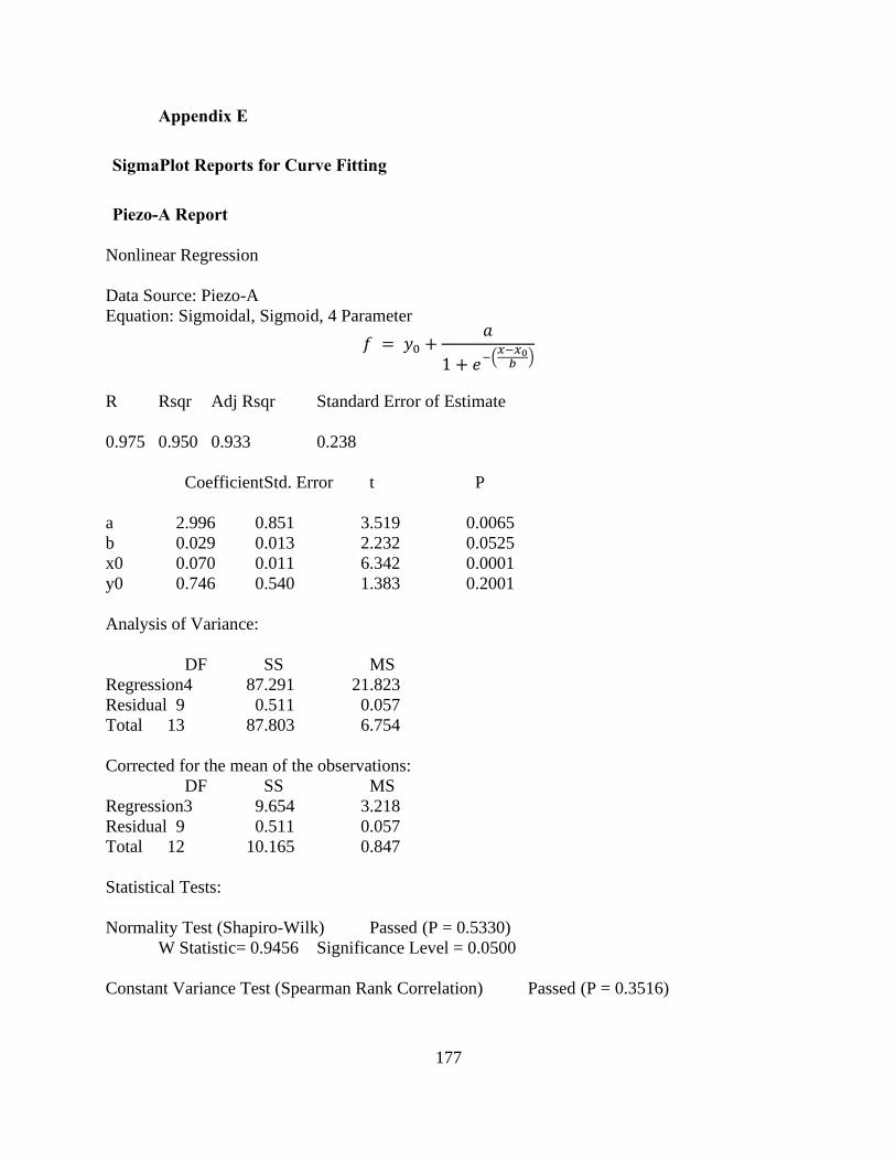
177
Appendix E
SigmaPlot Reports for Curve Fitting
Piezo-A Report
Nonlinear Regression
Data Source: Piezo-A
Equation: Sigmoidal, Sigmoid, 4 Parameter
𝑓 = 𝑦0 +𝑎
1 + 𝑒−(𝑥−𝑥0𝑏
)
R Rsqr Adj Rsqr Standard Error of Estimate
0.975 0.950 0.933 0.238
CoefficientStd. Error t P
a 2.996 0.851 3.519 0.0065
b 0.029 0.013 2.232 0.0525
x0 0.070 0.011 6.342 0.0001
y0 0.746 0.540 1.383 0.2001
Analysis of Variance:
DF SS MS
Regression4 87.291 21.823
Residual 9 0.511 0.057
Total 13 87.803 6.754
Corrected for the mean of the observations:
DF SS MS
Regression3 9.654 3.218
Residual 9 0.511 0.057
Total 12 10.165 0.847
Statistical Tests:
Normality Test (Shapiro-Wilk) Passed (P = 0.5330)
W Statistic= 0.9456 Significance Level = 0.0500
Constant Variance Test (Spearman Rank Correlation) Passed (P = 0.3516)

178
Fit Equation Description:
[Variables]
x = col(22)
y = col(23)
reciprocal_y = 1/abs(y)
reciprocal_ysquare = 1/y^2
reciprocal_x = 1/abs(x)
reciprocal_xsquare = 1/x^2
reciprocal_pred = 1/abs(f)
reciprocal_predsqr = 1/f^2
weight_Cauchy = 1/(1+4*(y-f)^2)
[Parameters]
a = 5 ' previous: 2.99641
b = 0.0444179 ' previous: 0.0287865
x0 = 0.127955 ' previous: 0.0702089
y0 = 1.84026 ' previous: 0.746203
[Equation]
f = y0+a/(1+exp(-(x-x0)/b))
fit f to y
''fit f to y with weight reciprocal_pred
''fit f to y with weight reciprocal_y
''fit f to y with weight reciprocal_ysquare
''fit f to y with weight reciprocal_x
''fit f to y with weight reciprocal_xsquare
''fit f to y with weight reciprocal_predsqr
[Constraints]
y0>0
a<3
[Options]
tolerance=1e-10
stepsize=1
iterations=1000
Number of Iterations Performed = 11
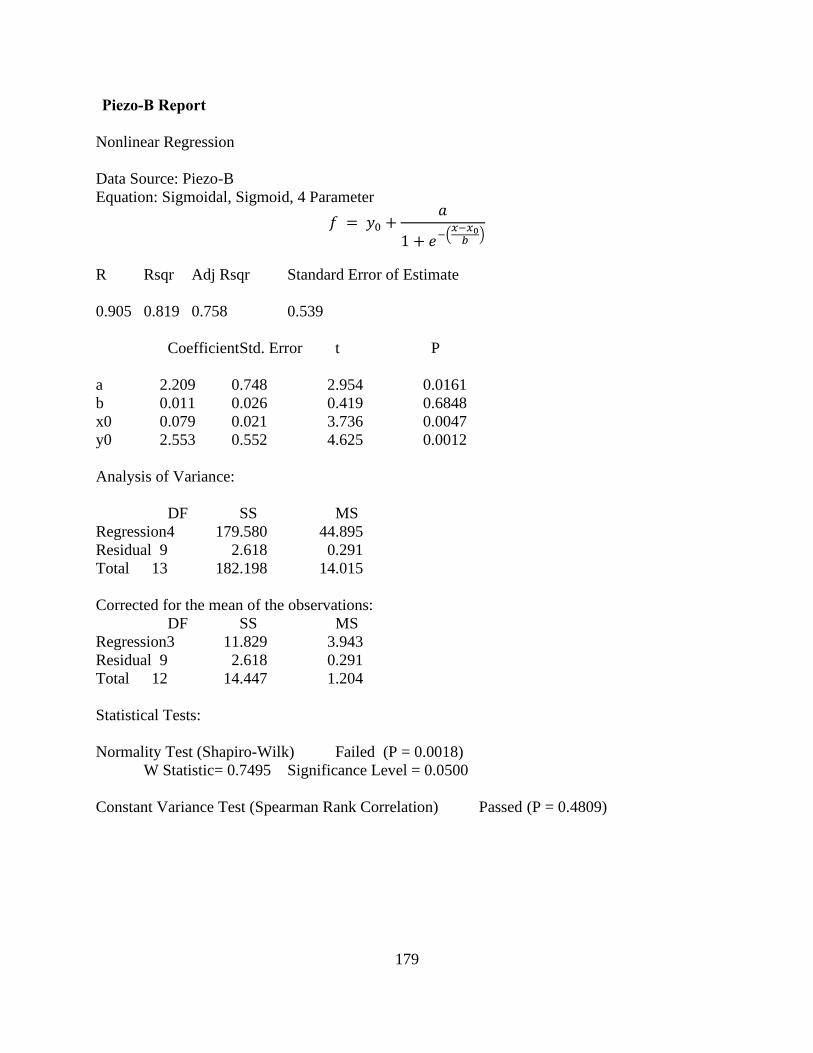
179
Piezo-B Report
Nonlinear Regression
Data Source: Piezo-B
Equation: Sigmoidal, Sigmoid, 4 Parameter
𝑓 = 𝑦0 +𝑎
1 + 𝑒−(𝑥−𝑥0𝑏
)
R Rsqr Adj Rsqr Standard Error of Estimate
0.905 0.819 0.758 0.539
CoefficientStd. Error t P
a 2.209 0.748 2.954 0.0161
b 0.011 0.026 0.419 0.6848
x0 0.079 0.021 3.736 0.0047
y0 2.553 0.552 4.625 0.0012
Analysis of Variance:
DF SS MS
Regression4 179.580 44.895
Residual 9 2.618 0.291
Total 13 182.198 14.015
Corrected for the mean of the observations:
DF SS MS
Regression3 11.829 3.943
Residual 9 2.618 0.291
Total 12 14.447 1.204
Statistical Tests:
Normality Test (Shapiro-Wilk) Failed (P = 0.0018)
W Statistic= 0.7495 Significance Level = 0.0500
Constant Variance Test (Spearman Rank Correlation) Passed (P = 0.4809)

180
Fit Equation Description:
[Variables]
x = col(22)
y = col(23)
reciprocal_y = 1/abs(y)
reciprocal_ysquare = 1/y^2
reciprocal_x = 1/abs(x)
reciprocal_xsquare = 1/x^2
reciprocal_pred = 1/abs(f)
reciprocal_predsqr = 1/f^2
weight_Cauchy = 1/(1+4*(y-f)^2)
[Parameters]
a = max(y)-min(y) ''Auto previous: 2.20881
b = if(xwtr(x,y-min(y),.5)<>0, xwtr(x,y-min(y),.5)/4, 1) ''Auto previous: 0.010873
x0 = x50(x,y-min(y),.5) ''Auto previous: 0.0789339
y0 = min(y) ''Auto previous: 2.55263
[Equation]
f = y0+a/(1+exp(-(x-x0)/b))
fit f to y
''fit f to y with weight reciprocal_y
''fit f to y with weight reciprocal_ysquare
''fit f to y with weight reciprocal_x
''fit f to y with weight reciprocal_xsquare
''fit f to y with weight reciprocal_pred
''fit f to y with weight reciprocal_predsqr
''fit f to y with weight weight_Cauchy
[Constraints]
y0>0
[Options]
tolerance=1e-10
stepsize=1
iterations=200
Number of Iterations Performed = 9

181
Piezo-C Report
Nonlinear Regression
Data Source: Piezo-C
Equation: Sigmoidal, Sigmoid, 4 Parameter
𝑓 = 𝑦0 +𝑎
1 + 𝑒−(𝑥−𝑥0𝑏
)
R Rsqr Adj Rsqr Standard Error of Estimate
0.988 0.976 0.968 0.131
CoefficientStd. Error t P
a 1.953 0.823 2.375 0.0416
b 0.016 0.014 1.189 0.2650
x0 0.104 0.019 5.456 0.0004
y0 1.899 0.106 17.994 <0.0001
Analysis of Variance:
DF SS MS
Regression4 94.320 23.580
Residual 9 0.155 0.017
Total 13 94.474 7.267
Corrected for the mean of the observations:
DF SS MS
Regression3 6.226 2.075
Residual 9 0.155 0.017
Total 12 6.381 0.532
Statistical Tests:
Normality Test (Shapiro-Wilk) Passed (P = 0.5689)
W Statistic= 0.9480 Significance Level = 0.0500
Constant Variance Test (Spearman Rank Correlation) Passed (P = 0.7784)

182
Fit Equation Description:
[Variables]
x = col(22)
y = col(23)
reciprocal_y = 1/abs(y)
reciprocal_ysquare = 1/y^2
reciprocal_x = 1/abs(x)
reciprocal_xsquare = 1/x^2
reciprocal_pred = 1/abs(f)
reciprocal_predsqr = 1/f^2
weight_Cauchy = 1/(1+4*(y-f)^2)
[Parameters]
a = max(y)-min(y) ''Auto previous: 1.95334
b = if(xwtr(x,y-min(y),.5)<>0, xwtr(x,y-min(y),.5)/4, 1) ''Auto previous: 0.0164483
x0 = x50(x,y-min(y),.5) ''Auto previous: 0.103582
y0 = min(y) ''Auto previous: 1.89879
[Equation]
f = y0+a/(1+exp(-(x-x0)/b))
fit f to y
''fit f to y with weight reciprocal_y
''fit f to y with weight reciprocal_ysquare
''fit f to y with weight reciprocal_x
''fit f to y with weight reciprocal_xsquare
''fit f to y with weight reciprocal_pred
''fit f to y with weight reciprocal_predsqr
''fit f to y with weight weight_Cauchy
[Constraints]
y0>0
[Options]
tolerance=1e-10
stepsize=1
iterations=200
Number of Iterations Performed = 11
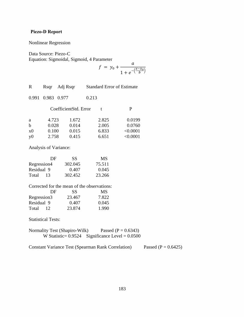
183
Piezo-D Report
Nonlinear Regression
Data Source: Piezo-C
Equation: Sigmoidal, Sigmoid, 4 Parameter
𝑓 = 𝑦0 +𝑎
1 + 𝑒−(𝑥−𝑥0𝑏
)
R Rsqr Adj Rsqr Standard Error of Estimate
0.991 0.983 0.977 0.213
CoefficientStd. Error t P
a 4.723 1.672 2.825 0.0199
b 0.028 0.014 2.005 0.0760
x0 0.100 0.015 6.833 <0.0001
y0 2.758 0.415 6.651 <0.0001
Analysis of Variance:
DF SS MS
Regression4 302.045 75.511
Residual 9 0.407 0.045
Total 13 302.452 23.266
Corrected for the mean of the observations:
DF SS MS
Regression3 23.467 7.822
Residual 9 0.407 0.045
Total 12 23.874 1.990
Statistical Tests:
Normality Test (Shapiro-Wilk) Passed (P = 0.6343)
W Statistic= 0.9524 Significance Level = 0.0500
Constant Variance Test (Spearman Rank Correlation) Passed (P = 0.6425)

184
Fit Equation Description:
[Variables]
x = col(22)
y = col(23)
reciprocal_y = 1/abs(y)
reciprocal_ysquare = 1/y^2
reciprocal_x = 1/abs(x)
reciprocal_xsquare = 1/x^2
reciprocal_pred = 1/abs(f)
reciprocal_predsqr = 1/f^2
weight_Cauchy = 1/(1+4*(y-f)^2)
[Parameters]
a = max(y)-min(y) ''Auto previous: 4.72262
b = if(xwtr(x,y-min(y),.5)<>0, xwtr(x,y-min(y),.5)/4, 1) ''Auto previous: 0.0282459
x0 = x50(x,y-min(y),.5) ''Auto previous: 0.0996556
y0 = min(y) ''Auto previous: 2.7577
[Equation]
f = y0+a/(1+exp(-(x-x0)/b))
fit f to y
''fit f to y with weight reciprocal_y
''fit f to y with weight reciprocal_ysquare
''fit f to y with weight reciprocal_x
''fit f to y with weight reciprocal_xsquare
''fit f to y with weight reciprocal_pred
''fit f to y with weight reciprocal_predsqr
''fit f to y with weight weight_Cauchy
[Constraints]
y0>0
[Options]
tolerance=1e-10
stepsize=1
iterations=200
Number of Iterations Performed = 11

185
Piezo-E Report
Nonlinear Regression
Data Source: Piezo-C
Equation: Sigmoidal, Sigmoid, 4 Parameter
𝑓 = 𝑦0 +𝑎
1 + 𝑒−(𝑥−𝑥0𝑏
)
R Rsqr Adj Rsqr Standard Error of Estimate
0.990 0.980 0.969 0.851
CoefficientStd. Error t P
a 20.056 6.012 3.336 0.0157
b 0.037 0.014 2.559 0.0430
x0 0.055 0.013 4.088 0.0064
y0 7.472E-0094.228 1.767E-009 1.0000
Analysis of Variance:
DF SS MS
Regression4 1654.075 413.519
Residual 6 4.350 0.725
Total 10 1658.425 165.842
Corrected for the mean of the observations:
DF SS MS
Regression3 209.199 69.733
Residual 6 4.350 0.725
Total 9 213.549 23.728
Statistical Tests:
Normality Test (Shapiro-Wilk) Passed (P = 0.7568)
W Statistic= 0.9575 Significance Level = 0.0500
Constant Variance Test (Spearman Rank Correlation) Passed (P = 0.3090)

186
Fit Equation Description:
[Variables]
x = col(22)
y = col(23)
reciprocal_y = 1/abs(y)
reciprocal_ysquare = 1/y^2
reciprocal_x = 1/abs(x)
reciprocal_xsquare = 1/x^2
reciprocal_pred = 1/abs(f)
reciprocal_predsqr = 1/f^2
weight_Cauchy = 1/(1+4*(y-f)^2)
[Parameters]
a = max(y)-min(y) ''Auto previous: 20.056
b = if(xwtr(x,y-min(y),.5)<>0, xwtr(x,y-min(y),.5)/4, 1) ''Auto previous: 0.0367937
x0 = x50(x,y-min(y),.5) ''Auto previous: 0.0547703
y0 = min(y) ''Auto previous: 7.47235e-009
[Equation]
f = y0+a/(1+exp(-(x-x0)/b))
fit f to y
''fit f to y with weight reciprocal_y
''fit f to y with weight reciprocal_ysquare
''fit f to y with weight reciprocal_x
''fit f to y with weight reciprocal_xsquare
''fit f to y with weight reciprocal_pred
''fit f to y with weight reciprocal_predsqr
''fit f to y with weight weight_Cauchy
[Constraints]
y0>0
[Options]
tolerance=1e-10
stepsize=1
iterations=200
Number of Iterations Performed = 10

187
Piezo-F Report
Nonlinear Regression
Data Source: Piezo-C
Equation: Sigmoidal, Sigmoid, 4 Parameter
𝑓 = 𝑦0 +𝑎
1 + 𝑒−(𝑥−𝑥0𝑏
)
R Rsqr Adj Rsqr Standard Error of Estimate
0.993 0.987 0.983 0.154
CoefficientStd. Error t P
a 3.751 0.378 9.932 <0.0001
b 0.023 0.004 6.322 0.0001
x0 0.050 0.005 10.616 <0.0001
y0 0.749 0.317 2.363 0.0424
Analysis of Variance:
DF SS MS
Regression4 158.390 39.598
Residual 9 0.213 0.024
Total 13 158.603 12.200
Corrected for the mean of the observations:
DF SS MS
Regression3 16.020 5.340
Residual 9 0.213 0.024
Total 12 16.232 1.353
Statistical Tests:
Normality Test (Shapiro-Wilk) Passed (P = 0.7670)
W Statistic= 0.9609 Significance Level = 0.0500
Constant Variance Test (Spearman Rank Correlation) Passed (P = 0.3616)

188
Fit Equation Description:
[Variables]
x = col(22)
y = col(23)
reciprocal_y = 1/abs(y)
reciprocal_ysquare = 1/y^2
reciprocal_x = 1/abs(x)
reciprocal_xsquare = 1/x^2
reciprocal_pred = 1/abs(f)
reciprocal_predsqr = 1/f^2
weight_Cauchy = 1/(1+4*(y-f)^2)
[Parameters]
a = max(y)-min(y) ''Auto previous: 3.75068
b = if(xwtr(x,y-min(y),.5)<>0, xwtr(x,y-min(y),.5)/4, 1) ''Auto previous: 0.0228536
x0 = x50(x,y-min(y),.5) ''Auto previous: 0.0501531
y0 = min(y) ''Auto previous: 0.74901
[Equation]
f = y0+a/(1+exp(-(x-x0)/b))
fit f to y
''fit f to y with weight reciprocal_y
''fit f to y with weight reciprocal_ysquare
''fit f to y with weight reciprocal_x
''fit f to y with weight reciprocal_xsquare
''fit f to y with weight reciprocal_pred
''fit f to y with weight reciprocal_predsqr
''fit f to y with weight weight_Cauchy
[Constraints]
y0>0
[Options]
tolerance=1e-10
stepsize=1
iterations=200
Number of Iterations Performed = 10
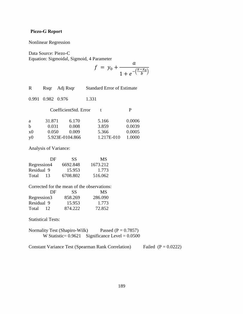
189
Piezo-G Report
Nonlinear Regression
Data Source: Piezo-C
Equation: Sigmoidal, Sigmoid, 4 Parameter
𝑓 = 𝑦0 +𝑎
1 + 𝑒−(𝑥−𝑥0𝑏
)
R Rsqr Adj Rsqr Standard Error of Estimate
0.991 0.982 0.976 1.331
CoefficientStd. Error t P
a 31.871 6.170 5.166 0.0006
b 0.031 0.008 3.859 0.0039
x0 0.050 0.009 5.366 0.0005
y0 5.923E-0104.866 1.217E-010 1.0000
Analysis of Variance:
DF SS MS
Regression4 6692.848 1673.212
Residual 9 15.953 1.773
Total 13 6708.802 516.062
Corrected for the mean of the observations:
DF SS MS
Regression3 858.269 286.090
Residual 9 15.953 1.773
Total 12 874.222 72.852
Statistical Tests:
Normality Test (Shapiro-Wilk) Passed (P = 0.7857)
W Statistic= 0.9621 Significance Level = 0.0500
Constant Variance Test (Spearman Rank Correlation) Failed (P = 0.0222)

190
Fit Equation Description:
[Variables]
x = col(22)
y = col(23)
reciprocal_y = 1/abs(y)
reciprocal_ysquare = 1/y^2
reciprocal_x = 1/abs(x)
reciprocal_xsquare = 1/x^2
reciprocal_pred = 1/abs(f)
reciprocal_predsqr = 1/f^2
weight_Cauchy = 1/(1+4*(y-f)^2)
[Parameters]
a = max(y)-min(y) ''Auto previous: 31.8714
b = if(xwtr(x,y-min(y),.5)<>0, xwtr(x,y-min(y),.5)/4, 1) ''Auto previous: 0.0312856
x0 = x50(x,y-min(y),.5) ''Auto previous: 0.0499244
y0 = min(y) ''Auto previous: 5.92275e-010
[Equation]
f = y0+a/(1+exp(-(x-x0)/b))
fit f to y
''fit f to y with weight reciprocal_y
''fit f to y with weight reciprocal_ysquare
''fit f to y with weight reciprocal_x
''fit f to y with weight reciprocal_xsquare
''fit f to y with weight reciprocal_pred
''fit f to y with weight reciprocal_predsqr
''fit f to y with weight weight_Cauchy
[Constraints]
y0>0
[Options]
tolerance=1e-10
stepsize=1
iterations=200
Number of Iterations Performed = 13

191
Piezo-H Report
Nonlinear Regression
Data Source: Piezo-C
Equation: Sigmoidal, Sigmoid, 4 Parameter
𝑓 = 𝑦0 +𝑎
1 + 𝑒−(𝑥−𝑥0𝑏
)
R Rsqr Adj Rsqr Standard Error of Estimate
0.978 0.956 0.937 0.292
CoefficientStd. Error t P
a 3.000 2.049 1.464 0.1865
b 0.016 0.029 0.537 0.6078
x0 0.098 0.030 3.288 0.0133
y0 2.160 0.339 6.368 0.0004
Analysis of Variance:
DF SS MS
Regression4 131.424 32.856
Residual 7 0.595 0.085
Total 11 132.019 12.002
Corrected for the mean of the observations:
DF SS MS
Regression3 12.857 4.286
Residual 7 0.595 0.085
Total 10 13.452 1.345
Statistical Tests:
Normality Test (Shapiro-Wilk) Passed (P = 0.3609)
W Statistic= 0.9248 Significance Level = 0.0500
Constant Variance Test (Spearman Rank Correlation) Passed (P = 0.3100)

192
Fit Equation Description:
[Variables]
x = col(22)
y = col(23)
reciprocal_y = 1/abs(y)
reciprocal_ysquare = 1/y^2
reciprocal_x = 1/abs(x)
reciprocal_xsquare = 1/x^2
reciprocal_pred = 1/abs(f)
reciprocal_predsqr = 1/f^2
weight_Cauchy = 1/(1+4*(y-f)^2)
[Parameters]
a = 5 ' previous: 3
b = 0.0444179 ' previous: 0.015642
x0 = 0.127955 ' previous: 0.0982315
y0 = 1.84026 ' previous: 2.16037
[Equation]
f = y0+a/(1+exp(-(x-x0)/b))
fit f to y
''fit f to y with weight reciprocal_y
''fit f to y with weight reciprocal_ysquare
''fit f to y with weight reciprocal_x
''fit f to y with weight reciprocal_xsquare
''fit f to y with weight reciprocal_pred
''fit f to y with weight reciprocal_predsqr
[Constraints]
y0>0
a<3
[Options]
tolerance=1e-10
stepsize=1
iterations=1000
Number of Iterations Performed = 8

193
Empirical equation Report
N = 96 Missing Observations = 16
R = 0.767 Rsqr = 0.588 Adj Rsqr = 0.575
Standard Error of Estimate = 0.230
Coefficient Std. Error t P VIF
Constant 1.291 0.222 5.822 <0.001
A/t [mm^2/mm] -0.479 0.0914 -5.244 <0.001 1.003
R [mm/mm] 0.638 0.0742 8.592 <0.001 1.003
v [m/s] 0.487 0.0997 4.890 <0.001 1.000
Analysis of Variance:
DF SS MS F P
Regression 3 6.928 2.309 43.802 <0.001
Residual 92 4.851 0.0527
Total 95 11.779 0.124
Column SSIncr SSMarg
A/t [mm^2/mm] 1.723 1.450
R [mm/mm] 3.945 3.892
v [m/s] 1.261 1.261
The dependent variable V [mV] can be predicted from a linear combination of the independent variables:
P
A/t [mm^2/mm] <0.001
R [mm/mm] <0.001
v [m/s] <0.001
All independent variables appear to contribute to predicting V [mV] (P < 0.05).
Normality Test (Shapiro-Wilk) Passed (P = 0.130)
Constant Variance Test (Spearman Rank Correlation): Passed (P = 0.113)
Power of performed test with alpha = 0.050: 1.000
=================
Regression Diagnostics:
=================
Row Predicted
1 0.654
2 0.423
3 0.363
4 0.507
5 0.582
6 0.602
7 1.132
8 0.266
9 0.627
10 0.423
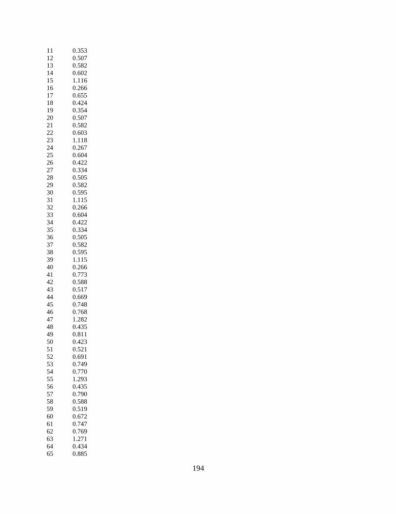
194
11 0.353
12 0.507
13 0.582
14 0.602
15 1.116
16 0.266
17 0.655
18 0.424
19 0.354
20 0.507
21 0.582
22 0.603
23 1.118
24 0.267
25 0.604
26 0.422
27 0.334
28 0.505
29 0.582
30 0.595
31 1.115
32 0.266
33 0.604
34 0.422
35 0.334
36 0.505
37 0.582
38 0.595
39 1.115
40 0.266
41 0.773
42 0.588
43 0.517
44 0.669
45 0.748
46 0.768
47 1.282
48 0.435
49 0.811
50 0.423
51 0.521
52 0.691
53 0.749
54 0.770
55 1.293
56 0.435
57 0.790
58 0.588
59 0.519
60 0.672
61 0.747
62 0.769
63 1.271
64 0.434
65 0.885
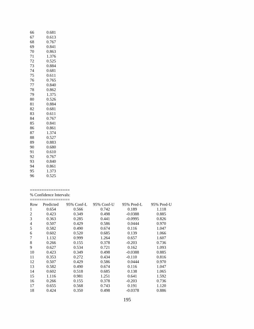
195
66 0.681
67 0.613
68 0.767
69 0.841
70 0.863
71 1.376
72 0.525
73 0.884
74 0.681
75 0.611
76 0.765
77 0.840
78 0.862
79 1.375
80 0.526
81 0.884
82 0.681
83 0.611
84 0.767
85 0.841
86 0.861
87 1.374
88 0.527
89 0.883
90 0.680
91 0.610
92 0.767
93 0.840
94 0.861
95 1.373
96 0.525
=================
% Confidence Intervals:
=================
Row Predicted 95% Conf-L 95% Conf-U 95% Pred-L 95% Pred-U
1 0.654 0.566 0.742 0.189 1.118
2 0.423 0.349 0.498 -0.0388 0.885
3 0.363 0.285 0.441 -0.0995 0.826
4 0.507 0.429 0.586 0.0444 0.970
5 0.582 0.490 0.674 0.116 1.047
6 0.602 0.520 0.685 0.139 1.066
7 1.132 0.999 1.264 0.657 1.607
8 0.266 0.155 0.378 -0.203 0.736
9 0.627 0.534 0.721 0.162 1.093
10 0.423 0.349 0.498 -0.0388 0.885
11 0.353 0.272 0.434 -0.110 0.816
12 0.507 0.429 0.586 0.0444 0.970
13 0.582 0.490 0.674 0.116 1.047
14 0.602 0.518 0.685 0.138 1.065
15 1.116 0.981 1.251 0.641 1.592
16 0.266 0.155 0.378 -0.203 0.736
17 0.655 0.568 0.743 0.191 1.120
18 0.424 0.350 0.498 -0.0378 0.886
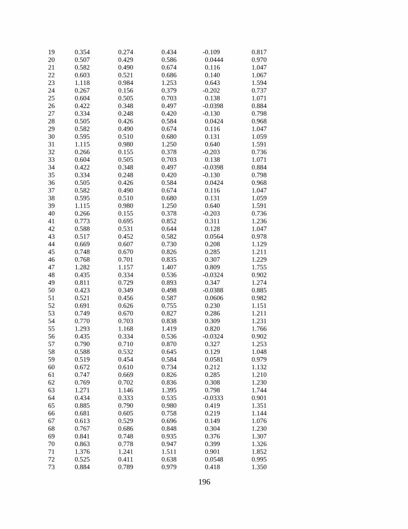
196
19 0.354 0.274 0.434 -0.109 0.817
20 0.507 0.429 0.586 0.0444 0.970
21 0.582 0.490 0.674 0.116 1.047
22 0.603 0.521 0.686 0.140 1.067
23 1.118 0.984 1.253 0.643 1.594
24 0.267 0.156 0.379 -0.202 0.737
25 0.604 0.505 0.703 0.138 1.071
26 0.422 0.348 0.497 -0.0398 0.884
27 0.334 0.248 0.420 -0.130 0.798
28 0.505 0.426 0.584 0.0424 0.968
29 0.582 0.490 0.674 0.116 1.047
30 0.595 0.510 0.680 0.131 1.059
31 1.115 0.980 1.250 0.640 1.591
32 0.266 0.155 0.378 -0.203 0.736
33 0.604 0.505 0.703 0.138 1.071
34 0.422 0.348 0.497 -0.0398 0.884
35 0.334 0.248 0.420 -0.130 0.798
36 0.505 0.426 0.584 0.0424 0.968
37 0.582 0.490 0.674 0.116 1.047
38 0.595 0.510 0.680 0.131 1.059
39 1.115 0.980 1.250 0.640 1.591
40 0.266 0.155 0.378 -0.203 0.736
41 0.773 0.695 0.852 0.311 1.236
42 0.588 0.531 0.644 0.128 1.047
43 0.517 0.452 0.582 0.0564 0.978
44 0.669 0.607 0.730 0.208 1.129
45 0.748 0.670 0.826 0.285 1.211
46 0.768 0.701 0.835 0.307 1.229
47 1.282 1.157 1.407 0.809 1.755
48 0.435 0.334 0.536 -0.0324 0.902
49 0.811 0.729 0.893 0.347 1.274
50 0.423 0.349 0.498 -0.0388 0.885
51 0.521 0.456 0.587 0.0606 0.982
52 0.691 0.626 0.755 0.230 1.151
53 0.749 0.670 0.827 0.286 1.211
54 0.770 0.703 0.838 0.309 1.231
55 1.293 1.168 1.419 0.820 1.766
56 0.435 0.334 0.536 -0.0324 0.902
57 0.790 0.710 0.870 0.327 1.253
58 0.588 0.532 0.645 0.129 1.048
59 0.519 0.454 0.584 0.0581 0.979
60 0.672 0.610 0.734 0.212 1.132
61 0.747 0.669 0.826 0.285 1.210
62 0.769 0.702 0.836 0.308 1.230
63 1.271 1.146 1.395 0.798 1.744
64 0.434 0.333 0.535 -0.0333 0.901
65 0.885 0.790 0.980 0.419 1.351
66 0.681 0.605 0.758 0.219 1.144
67 0.613 0.529 0.696 0.149 1.076
68 0.767 0.686 0.848 0.304 1.230
69 0.841 0.748 0.935 0.376 1.307
70 0.863 0.778 0.947 0.399 1.326
71 1.376 1.241 1.511 0.901 1.852
72 0.525 0.411 0.638 0.0548 0.995
73 0.884 0.789 0.979 0.418 1.350
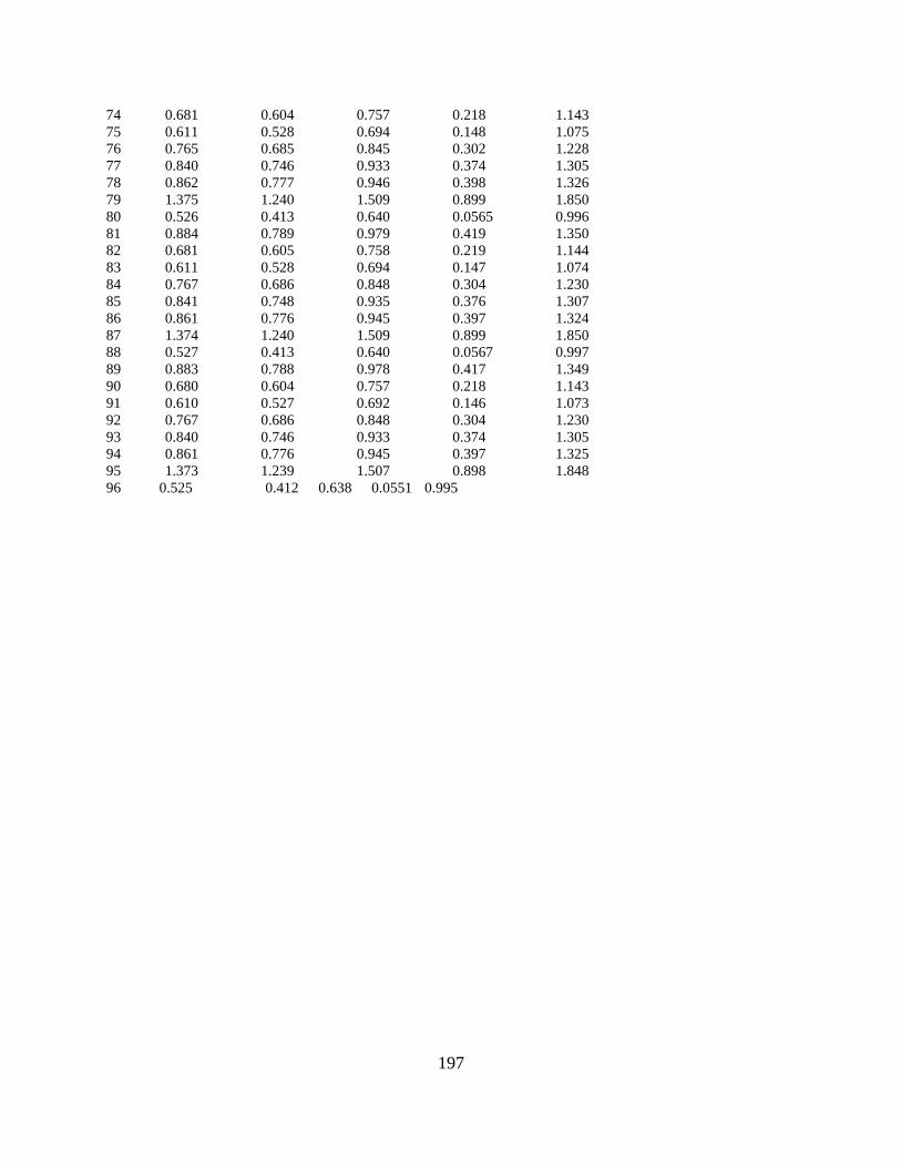
197
74 0.681 0.604 0.757 0.218 1.143
75 0.611 0.528 0.694 0.148 1.075
76 0.765 0.685 0.845 0.302 1.228
77 0.840 0.746 0.933 0.374 1.305
78 0.862 0.777 0.946 0.398 1.326
79 1.375 1.240 1.509 0.899 1.850
80 0.526 0.413 0.640 0.0565 0.996
81 0.884 0.789 0.979 0.419 1.350
82 0.681 0.605 0.758 0.219 1.144
83 0.611 0.528 0.694 0.147 1.074
84 0.767 0.686 0.848 0.304 1.230
85 0.841 0.748 0.935 0.376 1.307
86 0.861 0.776 0.945 0.397 1.324
87 1.374 1.240 1.509 0.899 1.850
88 0.527 0.413 0.640 0.0567 0.997
89 0.883 0.788 0.978 0.417 1.349
90 0.680 0.604 0.757 0.218 1.143
91 0.610 0.527 0.692 0.146 1.073
92 0.767 0.686 0.848 0.304 1.230
93 0.840 0.746 0.933 0.374 1.305
94 0.861 0.776 0.945 0.397 1.325
95 1.373 1.239 1.507 0.898 1.848
96 0.525 0.412 0.638 0.0551 0.995
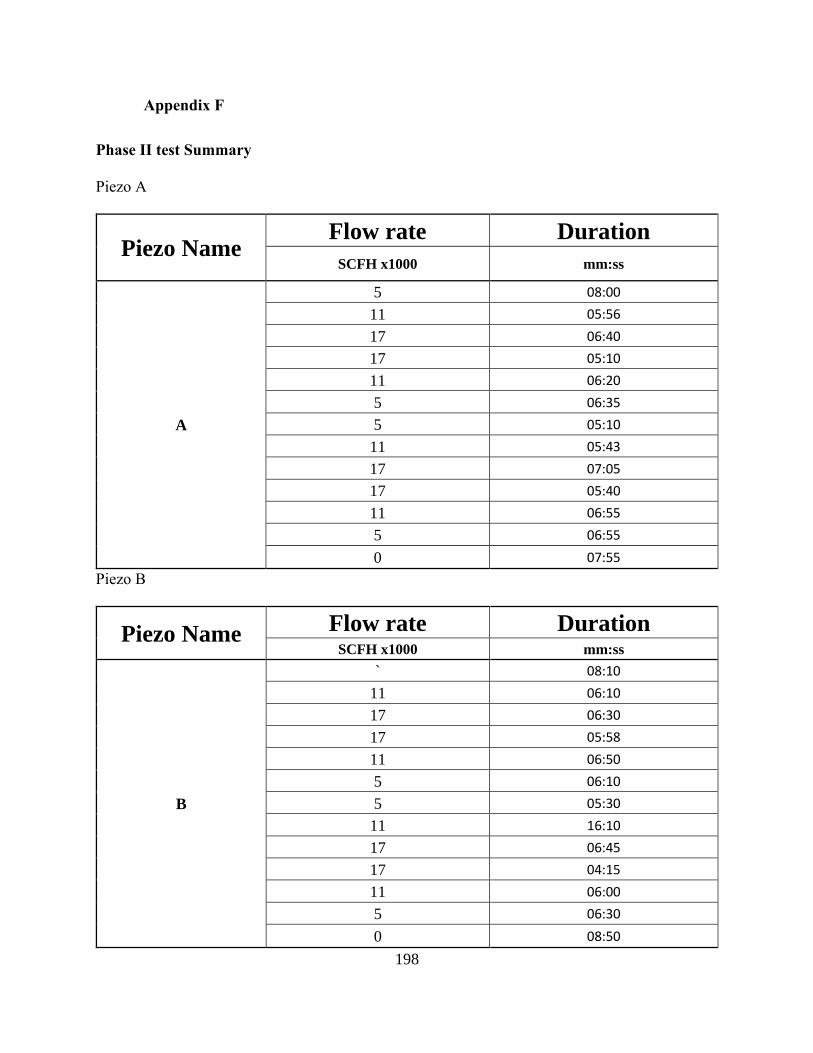
198
Appendix F
Phase II test Summary
Piezo A
Piezo Name Flow rate Duration
SCFH x1000 mm:ss
A
5 08:00
11 05:56
17 06:40
17 05:10
11 06:20
5 06:35
5 05:10
11 05:43
17 07:05
17 05:40
11 06:55
5 06:55
0 07:55
Piezo B
Piezo Name Flow rate Duration
SCFH x1000 mm:ss
B
` 08:10
11 06:10
17 06:30
17 05:58
11 06:50
5 06:10
5 05:30
11 16:10
17 06:45
17 04:15
11 06:00
5 06:30
0 08:50
199
Piezo C
Piezo Name Flow rate Duration
SCFH x1000 mm:ss
C
5 08:15
11 06:10
17 07:13
17 05:53
11 07:05
5 07:30
5 06:05
11 06:30
17 06:55
17 04:54
11 07:15
5 07:15
0 07:25
Piezo D
Piezo Name Flow rate Duration
SCFH x1000 mm:ss
D
5 05:00
11 05:00
17 06:45
17 05:00
11 06:00
5 05:45
5 05:00
11 05:30
17 04:25
17 05:00
11 05:30
5 05:15
0 07:00
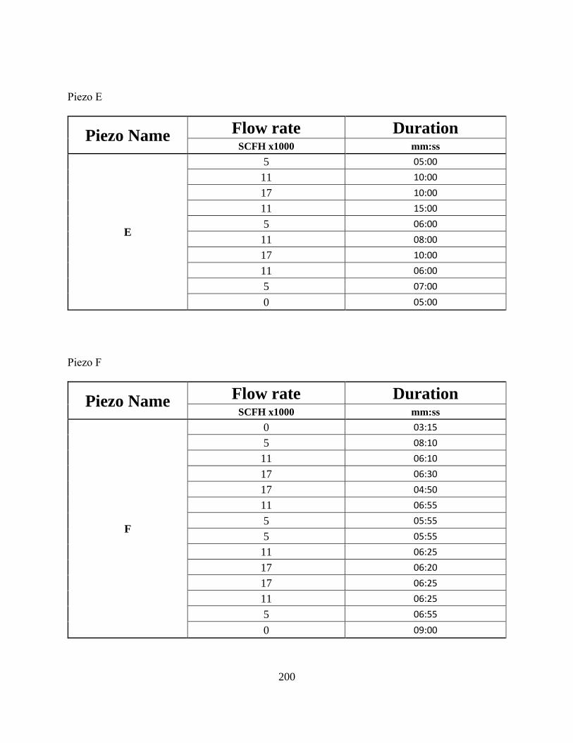
200
Piezo E
Piezo Name Flow rate Duration
SCFH x1000 mm:ss
E
5 05:00
11 10:00
17 10:00
11 15:00
5 06:00
11 08:00
17 10:00
11 06:00
5 07:00
0 05:00
Piezo F
Piezo Name Flow rate Duration
SCFH x1000 mm:ss
F
0 03:15
5 08:10
11 06:10
17 06:30
17 04:50
11 06:55
5 05:55
5 05:55
11 06:25
17 06:20
17 06:25
11 06:25
5 06:55
0 09:00
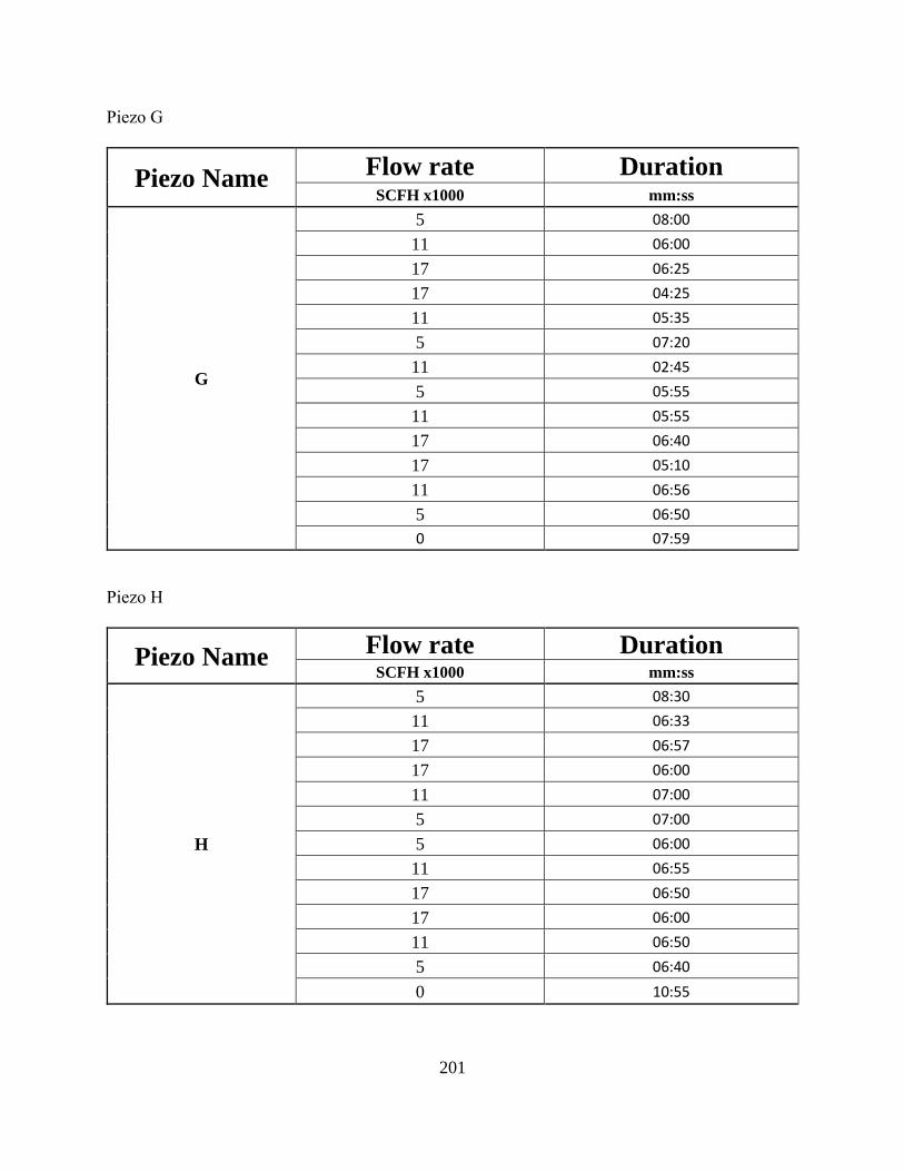
201
Piezo G
Piezo Name Flow rate Duration
SCFH x1000 mm:ss
G
5 08:00
11 06:00
17 06:25
17 04:25
11 05:35
5 07:20
11 02:45
5 05:55
11 05:55
17 06:40
17 05:10
11 06:56
5 06:50
0 07:59
Piezo H
Piezo Name Flow rate Duration
SCFH x1000 mm:ss
H
5 08:30
11 06:33
17 06:57
17 06:00
11 07:00
5 07:00
5 06:00
11 06:55
17 06:50
17 06:00
11 06:50
5 06:40
0 10:55

202
Vita
Jad G. Aboud joined the University of Texas at El Paso (UTEP) in Fall 2012 as an
undergraduate student in Mechanical Engineering. During his study, he volunteered in
Musculoskeletal Lab, and he has been an active member of the University organizations as well.
Besides, he was on the dean’s list from 2012 to 2015 for each semester. He was selected as a team
leader for the joiner and senior projects. Jad graduated from the program with a GPA of 3.79, and
upon his graduation in Spring 2015, he was awarded the Superior Achievement Award for
exceptional performance throughout his undergraduate studies. After that, he joined the College
of Engineering graduate program to aspire to further aerospace and combustion studies. From an
undergraduate to a Graduate Research Assistant at the Center for Space Exploration Technology
Research Lab (cSETR) under the supervision of Dr. Norman Love Jr., Jad’s primary research
interest opened the doors for a collaboration with other researchers to design, model, and test a
supersonic, liquid-cooled combustor intended to be used in a direct power extraction system.
During the project, his work resulted in three publications and was awarded the best paper by the
AIAA Terrestrial Committee at the 2016 SciTech Conference in San Diego, California. He
graduated from the Master of Science program with a GPA of 3.9. Jad pursued his Doctor of
Philosophy in the Mechanical Engineering Program to succeed in this field. During his study, he
continued working in cSETR as a graduate research assistant. He was selected as a team leader.
Jad was selected for two internships at NETL in Albany, Oregon, and Morgantown, West Vergina,
though CIESESE and MLEF. His work resulted in a provisional patent number 17/100, 4094. After
graduation, Jad will pursue a job in the aerospace industry to succeed in this field.
Contact Information: [email protected]