Effectiveness of History-Dependent Monetary Policy*

Takeshi Kimura** and Takushi Kurozumi***

Bank of Japan

First version : September 2001Revised : March 2002

* We are grateful for helpful discussions and comments from Kosuke Aoki, Makoto Saito, FrankSmets and Michael Woodford, as well as seminar participants at the third CIRJE/TCER macro-conference (the joint conference of the Center for International Research on the Japanese Economyand the Tokyo Center for Economic Research) and the ECB workshop on “The Role of Policy Rulesin the Conduct of Monetary Policy”. We would also like to thank Saori Sato for excellent researchassistance. All remaining errors are our own. The views expressed herein are those of the authorsalone and not necessarily those of the Bank of Japan.**

Policy Research Division, Policy Planning Office, Bank of Japan, e-mail: takeshi.kimura-1@boj.or.jp*** Policy Research Division, Policy Planning Office, Bank of Japan, e-mail: takushi.kurozumi@boj.or.jp

1

Summary

In this paper, we evaluate the effectiveness of history-dependent monetary policy, focusing on

the design of optimal delegation (targeting regime) and simple policy rules. Our quantitative

analysis is based on a small estimated forward-looking model of the Japanese economy with a

hybrid Phillips curve in which a fraction of firms use a backward-looking rule to set prices.

Using this model, we calculate social welfare losses under the alternative policy regimes, and

then compare their performance with that under the optimal commitment policy. Our main

findings are summarized as follows:

(1) An important characteristic of history-dependent policy is trend-reverting behavior of the

price level. Such price dynamics have an immediate effect of stabilizing inflation against price

shocks through the forward-looking expectations of private agents. However, when a fraction of

firms use a backward-looking rule to set prices, it is not optimal for the central bank to achieve

full trend-reversion of the price level. Instead, partial trend-reversion of the price level with

some degree of drift is desirable under the optimal commitment policy.

(2) Under history-dependent targeting regimes, such as price level targeting and nominal income

growth targeting, a discretionary central bank brings the price level back to its initial trend path

completely in the face of price shocks. Although such full trend-reversion of the price level is

not socially optimal, these targeting regimes achieve lower welfare losses and perform much

better than inflation targeting in which history dependence is not introduced. This is because

trend-reversion of the price level tends to move equilibrium toward what would be achieved

under the optimal commitment policy.

(3) Committing to a simple history-dependent policy rule also achieves lower welfare losses and

results in nearly the same performance as the optimal delegation of price level targeting and

income growth targeting. Among simple policy rules, the most efficient is the first difference

hybrid policy rule in which the change in interest rate responds to current inflation and both

current and past output gaps.

(4) By committing to the first difference hybrid policy rule, the central bank can achieve almost

the same performance as the optimal commitment policy. This is because the partial trend-

reverting behavior of the price level under the optimal policy can be replicated by the hybrid

rule.

Keywords : Monetary Policy, History Dependence, Delegation, Policy Rules, Commitment,Discretion, Inflation Targeting, Price Level Targeting, Income Growth Targeting

JEL Classification : E52, E58

2

1. Introduction

Recent monetary policy studies have emphasized the importance of history

dependence in the conduct of monetary policy. Giannoni (2000) and Woodford (2000) point

out that when private agents are forward-looking, it is optimal for the central bank not only

to respond to current shocks and the current state of the economy, but that it is also

desirable to respond to lagged variables. Conducting monetary policy of this kind allows the

central bank to appropriately affect private sector expectations. This, in turn, improves the

performance of monetary policy, because the evolution of the central bank’s target variables

depends not only on its current actions, but also on how the private sector foresees future

monetary policy.

Optimal commitment policy is history dependent and most efficient. However, it is

generally time-inconsistent and therefore not particularly realistic. A lot of previous

literature investigated other ways in which the monetary policy decision-making process

might incorporate the sort of history dependence required for the optimal commitment

policy. The design of optimal delegation is one way. On the assumption that the central

bank will pursue its goal in a discretionary fashion, rather than committing itself to an

optimal plan, the optimal goal with which to charge the central bank need not correspond to

the true social welfare function. It is desirable that the loss function assigned to the central

bank depend on lagged as well as current values of the target variables. In this case,

discretionary policy is history dependent because the bank’s loss function is history

dependent even though the true social loss function is not.

Vestin (2000) shows that, within a purely forward-looking Phillips curve, discretionary

optimization results in the same equilibrium as the optimal commitment policy, if the

central bank is charged with stabilization of the price level rather than the inflation rate.

Price level targeting is a history-dependent policy, in the sense that the central bank’s loss

function depends on the cumulative sum of inflation rates over past periods. Jensen (1999)

and Walsh (2001) show that discretionary income growth targeting is also desirable,

because the central bank’s loss function depends on lagged output gap as well as current

values of target variables.

However, there are several problems with the practical implementation of optimal

delegation. Optimal delegation regimes require full information with respect to demand and

price shocks for implementation by the central bank. When the central bank cannot

accurately observe these shocks, which seems to be a realistic assumption, optimal

3

delegation is not so effective as previous literature suggests. Even if the central bank can

completely identify these shocks, the policy reaction function implied by optimal delegation

is very complicated and not transparent to the public.

Instead of implementing optimal delegation, adopting a simple policy rule is another

way to incorporate history dependence into monetary policy. Woodford (1999,2000) and

Giannoni (2000) suggest that central banks can introduce desirable history dependence into

monetary policy by adopting a policy rule in which the interest rate reacts to its own lagged

value, price level, or income growth (i.e. change in output gap). Giannoni (2000) then

shows that such a simple history-dependent policy rule performs better than the Taylor rule

and results in lower welfare loss. Because simple policy rules involve no explicit

dependence on demand and price shocks, and so do not even require that the central bank

know these shocks, conducting monetary policy with emphasis on simple rules seems to be

a practical and transparent scheme.

Still, there remain several problems with respect to history-dependent policy, which

previous literature did not solve.

First, the effectiveness of history-dependent policy critically depends on the forward-

looking behavior of private agents. Giannoni (2000) and Vestin (2000) investigate history-

dependent policy with a purely forward-looking New Keynesian Phillips curve. However,

the New Keynesian Phillips curve has been criticized for failing to match the short-run

dynamics exhibited by inflation (see, for example, Mankiw (2000)). Specifically, inflation

seems to respond sluggishly and display significant persistence in the face of price shocks,

while the New Keynesian Phillips curve allows current inflation to be a jump variable that

can respond immediately to any disturbance. Therefore, in order to obtain the practical

implication of history-dependent policy, we must use a model with empirically plausible

amounts of forward-looking behavior and inflation persistence.

Second, previous literature indicated that history-dependent targeting regimes, such as

price level targeting and income growth targeting, outperform inflation targeting, but it is

not clear which history-dependent targeting regime performs better and to what degree the

performance of each targeting regime differs quantitatively. This is because the competing

regimes of delegation have been examined separately over different models.

Third, previous literature does not clarify which history-dependent policy regime

performs better, delegation (targeting regime) or a simple policy rule. Although a policy

regime based on a simple rule is transparent to the public, if it performs worse than optimal

4

delegation, then the policy rule regime is not desirable. On the other hand, if we can show

that simple policy rules which involve no explicit dependence on demand and price shocks

are as effective as optimal delegation, then it is more desirable than optimal delegation,

based on the realistic assumption that the central bank cannot observe these shocks

accurately.

Fourth, Giannoni (2000) derives a policy rule that implements the optimal commitment

policy in the purely forward-looking New Keynesian Phillips curve. However, this leaves

the problem of whether there is a simple policy rule which achieves the same performance

as the optimal commitment policy when endogenous persistence is incorporated in inflation

dynamics.

The purpose of this paper is to investigate history-dependent policy and attempt to

solve the above unresolved problems in a unified framework. Our quantitative analysis is

based on a small estimated forward-looking model of the Japanese economy with a hybrid

Phillips curve. This Phillips curve is a modified inflation adjustment equation which

incorporates endogenous persistence by including the lagged inflation rate in the New

Keynesian Phillips curve. That is, it nests the purely forward-looking Phillips curve as a

particular case, and allows for a fraction of firms that use a backward-looking rule to set

prices. Using this model, we calculate social welfare losses under the alternative policy

regimes, and then compare their performance with that under the optimal commitment

policy. Although we do not consider the optimal commitment policy particularly realistic, it

will serve as a useful benchmark against which policy under the alternative regimes can be

evaluated.

Our main findings are summarized as follows.

(1) According to the estimation results of the hybrid Phillips curve based on Japan’s data,

about 60% of firms exhibit forward-looking price setting behavior (i.e. the remaining 40%

of firms exhibit backward-looking behavior). Although the purely forward-looking

Phillips curve is rejected by the data, such a degree of forward-looking behavior seems to

be sufficient to make history-dependent policy effective.

(2) Indeed, history-dependent targeting regimes, such as income growth targeting and price

level targeting, outperform inflation targeting and result in lower social welfare losses. In

addition, the optimal commitment policy can be roughly replicated by delegating income

growth targeting to a conservative central bank, which values inflation stability more than

society does. The optimal commitment policy can also be roughly replicated by

5

delegating price level targeting to a liberal central bank, which values output stability

more than society does. Price level targeting and income growth targeting perform at

almost the same level.

(3) Simple history-dependent policy rules, such as a price level targeting rule and income

growth targeting rule, perform much better than the Taylor rule in which history

dependence is not introduced. Moreover, committing to such a history-dependent rule

results in nearly the same social welfare as the optimal delegation of price level targeting

and income growth targeting.

(4) Among simple history-dependent rules, the most efficient is the first difference hybrid

rule in which the change in interest rate responds to current inflation and both current and

past output gaps. By adopting this rule, the central bank can achieve almost the same

performance as the optimal commitment policy. Besides, this hybrid rule may be effective

even if the central bank is faced with the zero interest rate bound.

(5) The good performance of the first difference hybrid rule results from partial trend-

reverting behavior of the price level. Through the forward-looking expectations of private

agents, the trend-reversion of the price level has the immediate effect of stabilizing

inflation against price shocks. However, in the hybrid Phillips curve, it is not socially

optimal for the central bank to completely bring the price level back to its initial trend

path. This is because the central bank must pay the high cost of greater output gap

volatility to achieve full trend-reversion of the price level when a fraction of firms use a

backward-looking rule to set prices. Therefore, partial trend-reversion of the price level

with some degree of drift is desirable in the hybrid Phillips curve. Such partial trend-

reverting behavior of the price level can be replicated by the hybrid rule, but not by other

history-dependent rules.

The outline of the remainder of the paper is as follows. Section 2 presents the model of

the economy and poses the problem of optimal commitment and discretion policy. Section 3

presents the estimation results of the model. Then, using the estimated model, we show how

endogenous variables respond to shocks and calculate welfare losses under optimal policy.

Sections 4 and 5 present quantitative analysis of optimal delegation and simple policy rules

respectively. Finally, Section 6 provides concluding remarks.

6

2. Framework for Optimal Monetary Policy

This section first sets out a dynamic general equilibrium model, and then describes the

formal monetary policy design problem.

2.1. Model

The model economy is a particularly simple version of a dynamic general equilibrium

model that has been extensively applied in literature discussing monetary policy

evaluation.1 The model consists of two relationships: 1) an aggregate demand condition that

links output and the real interest rate, and 2) an inflation adjustment equation that links

inflation and output.

Aggregate demand is determined by the following intertemporal IS curve:

tttttttttttt ripEiyyEyyyy εσφφ +−∆−−−−+−=− ∗+

∗++

∗−−

∗ })][(][){1()( 11111 ,

δσ +∆= ∗+

−∗ ][ 11

ttt yEri , 10 <≤φ , ,0 σ< ,0 δ<

(1)

where ty and *ty are real output and potential real output, respectively, both in logs.

*ty is the

level of output that would arise if wages and prices were perfectly flexible, and thedifference between ty and

*ty ,

∗− tt yy , is an output gap. ti is the short-term nominal

interest rate assumed to be the monetary policy instrument. tp is the log price level, and itsfirst difference tp∆ is the inflation rate.

tE is the expectations operator conditional on all

information up to period t. tε is a demand shock representing an autonomous variation in

spending such as government spending. In the special case where 0=φ , equation (1)

approximates the path of demand arising from the Euler equation characterizing optimal

consumption choices by the representative household. Parameter σ can then be interpreted

as the rate of intertemporal substitution determining to what extent the real interest rate,][ 1+∆− ttt pEi , affects expected spending growth. ∗

tri is the equilibrium real interest rate,which is the sum of the expected potential growth rate ][ 1

∗+∆ tt yE (times the inverse of σ )

and time preference rate δ. For mainly empirical reasons, the IS curve specification allowsfor endogenous persistence in demand when 10 << φ . By appealing to some form of

adjustment costs, it may be feasible to explicitly motivate the appearance of lagged output

within the IS curve.

The inflation adjustment equation is modeled by the following Phillips curve: 1 See, for example, Clarida, Galí and Gertler (1999), Jensen (1999), Walsh (2001), Giannoni (2000),Rudebusch (2000), Smets (2000), Vestin (2000), and Woodford (1999,2000,2001).

7

ttttttt yypEpp µλβθθ +−+∆−+∆=∆ ∗+− )(][)1()( 11 , 10 <≤θ , 0>λ . (2)

In the special case where 0=θ , the structure of equation (2) resembles what Roberts (1995)

has labeled the “New Keynesian Phillips curve”, which can be derived from a variety of

supply-side models. For example, it can be described as the staggered price determination

that emerges from a monopolistically competitive firm’s optimal behavior in Calvo’s (1983)

model. Roughly speaking, firms set nominal prices based on the expectations of futuremarginal costs. The output gap

∗− tt yy captures movements in marginal costs associated

with variation in excess demand. The shock tµ , which we refer to as price shock, captures

anything else that might affect expected marginal costs. This could be caused, for example,

by movements in nominal wages that push real wages away from their equilibrium valuesdue to frictions in the wage contracting process.2 The presence of this price shock tµ is of

all importance for the ensuing analyses because it induces the trade-off in monetary

policymaking that matters in the design of optimal policy.

The New Keynesian Phillips curve, where 0=θ is assumed in equation (2), has been

criticized for failing to match the short-run dynamics exhibited by inflation.3 Specifically,

inflation seems to respond sluggishly and to display significant persistence in the face of

price shocks, while the New Keynesian Phillips curve allows current inflation to be a jump

variable that can immediately respond to any disturbance. Therefore, we introduce theendogenous inflation persistence in equation (2) by allowing for 10 <<θ . The inclusion of

the lagged inflation rate could be due to overlapping nominal contracts aimed at securing

real wage levels comparable to existing and expected real wages.4 Alternatively, it could be

due to the existence of firms that use a backward-looking rule to set prices.5 In the latter

case, equation (2) can be interpreted as the hybrid curve of the traditional backward-lookingPhillips curve and the New Keynesian Phillips curve, where the parameter θ depends on the

weight of backward-looking firms.

We assume that exogenous disturbances follow AR(1) processes:

,ˆ1 ttt εψ εε += − 11 <<− ψ (3)

,ˆ1 ttt µρµµ += − 11 <<− ρ (4)

2 See Erceg, Henderson and Levin (2000) for details.3 See, for example, Mankiw (2000).4 See Fuhrer and Moore (1995).5 See Galí and Gertler (1999).

8

,ˆ)1( *1

*ttt yy ξωτω +∆+−=∆ − 10 <≤ω (5)

τ is an average rate of potential growth. All stochastic innovations tε̂ , tµ̂ , and tξ̂ are white

noises and may be correlated with each other.

Finally, we note that our model may be applied to the open economy. Although our

model does not explicitly involve the exchange rate, Clarida, Galí and Gertler (2001) show

that the open economy can be simply modeled by equations (1)-(2) with the price of

domestic output pt as well as the terms of trade equation.

2.2. Optimal Monetary Policy

The policy regimes to be considered are evaluated according to a social welfare loss

function, which is assumed as follows:

10,10,})())(1{(0

2*2 ≤≤<<

−+∆−∑

∞

=+++ αβααβ

jjtjtjt

jt yypE , (6)

where β is a discount factor. This loss function is the unconditional expectation of the

discounted sum of quadratic deviations of output from potential and quadratic deviations of

inflation from a target of zero. The weight α reflects society’s preference for output

stabilization relative to inflation stabilization. As demonstrated by Woodford (2001), such a

social loss function can be derived as an approximation from the utility of a representative

household in the closed economy, when inflation dynamics can be described as the New

Keynesian Phillips curve (i.e. where 0=θ in equation (2)). Benigno and Benigno (2001)

suggest that where 0=θ , the social loss function in the open economy can also be

approximated as function (6) with the domestic price pt. Although function (6) may not be

an accurate approximation of social welfare in the case of the hybrid Phillips curve( 10 <<θ ), we simply adopt it because this formulation does not seem out of sync with the

way monetary policy operates in practice, at least implicitly. Indeed, function (6) has been

applied in virtually all literature on monetary policy issues in the past.6

6 As demonstrated by Steinsson (2000) and Amato and Laubach (2002), in the case of the hybridPhillips curve, the theoretical loss function includes the variability in the change of inflation as wellas inflation rate and output gap. However, the only effect of adding the variability of the change ininflation to the traditional loss function (6) is to increase the weight of inflation stabilization relativeto output gap stabilization, since any reduction of inflation variability reduces the variability of thechange in inflation as well. We analyze the whole range of society’s preference for inflationstabilization by using the traditional loss function (6). Therefore, using the theoretical loss functioninstead of the traditional one does not substantially influence the results of our analysis.

9

Given the social welfare loss function, it is possible –– and obviously optimal –– to

completely stabilize the output gap and inflation against demand and productivity shocks.

This follows immediately upon inspection of the IS curve (1) and the Phillips curve (2). By

adjusting the interest rate, any effect of demand and productivity shocks on the output gap

and thus inflation is completely eliminated. That is, these shocks do not constitute a policy

trade-off. In contrast, it is impossible to perfectly stabilize the output gap and inflation

against price shocks. This is also immediately seen by inspecting the Phillips curve (2). For

example, in the case of a positive price shock, inflationary pressures arise in the economy,

which can only be dampened through a contractionary policy reducing the output gap.

Therefore, the central bank faces a trade-off between stabilization of inflation and

stabilization of the output gap. While this mechanism is very straightforward, the optimal

way of responding to price shocks differs according to policy regime, as we show below.

2.2.1. Optimal Monetary Policy under Commitment

Consider the case where the central bank has complete credibility and is able to

commit. Thus, it can credibly announce any future path for the output gap and thus affect

private sector expectations about future inflation. The central bank’s problem is to minimize

the social loss function (6) subject to the hybrid Phillips curve (2).7 The first order

conditions for this problem are as follows:

[ ]][)()1( *11

*++ −−−−=∆− tttttt yyEyyp θβααλ , (7a)

[ ]][))(1()()1( ,1 *11

*11

*+++++−+−++++ −−−−−−−=∆−≥∀ jtjtjtjtjtjtjtjt yyEyyyypj θβθααλ . (7b)

It is easy to interpret the economic meaning of these conditions in the case of 0=θ ,

that is, when the inflation adjustment equation is described as the New Keynesian Phillips

curve. Condition (7a) simply implies that the central bank pursue a ‘lean against the wind’

policy: Whenever inflation is above the target rate of zero, reduce demand below capacity

(by raising the interest rate); and vice versa when below target. How aggressively the

central bank should reduce the output gap depends positively on the gain in reduced

7 What is critical in this optimization problem is the existence of price shock tµ in equation (2),which induces the trade-off between inflation stabilization and output gap stabilization. Since neitherdemand shock nor productivity shock induces such a tradeoff, the IS curve (1) is redundant for thisproblem. After the central bank chooses a path for both the inflation rate and output gap to minimizethe social loss function subject to equation (2), it then determines the interest rate implied by the ISequation (1), conditional on the optimal values of inflation rate and output gap. See Clarida, Galí andGertler (1999) for details.

10

inflation per unit of output loss,λ, and inversely on the relative weight placed on output

losses α . Condition (7b) implies, in the case of 0=θ , that optimal commitment requires

adjusting the change in the output gap in response to inflation. That is, optimal monetarypolicy is history dependent in that equation (7b) involves lagged output gap *

11 −+−+ − jtjt yy .

Such history dependence in monetary policy arises as a product of the central bank’s ability

under commitment to directly manipulate private sector expectations. To see this, keep in

mind that the inflation rate depends not only on the current output gap but also on the

expected future path of the output gap.8 Then suppose, for example, that there is a price

shock that raises inflation above target at time t. Optimal policy continues to reduce outputgap

∗++ − jtjt yy as long as jtp +∆ remains above target. The credible threat to continue to

contract the output gap in the future, in turn, has the immediate effect of dampening current

inflation, given the dependence of inflation rate on the future output gap.

Note that, in the case of 0=θ , the first order condition (7b) can be equivalently

expressed as

)())(1( ,1 *jtjtjt yyppj ++

∗+ −−=−−≥∀ ααλ , (8)

where

∗p is a constant target price level corresponding to the target rate of inflation, i.e. zero.

Thus, for example, the central bank commits to reduce demand when the price exceeds the

constant target level; hence, the trend-reverting behavior of the price level. This is an

important property of history dependent policy in the case of 0=θ .

Although it is not easy to interpret the economic meaning of equation (7b) in the case

of 0>θ , optimal monetary policy under commitment is history dependent as long as θ>1 ,because equation (7b) involves lagged output gap

*11 −+−+ − jtjt yy . This means that the

qualitative significance of history dependence in the conduct of monetary policy does existwhen expectations play a role (i.e. θ>1 ).

The first order conditions (7) reveal the importance of history dependence in the

optimal commitment policy, but this policy is generally not time-consistent in rational

expectations models. At time t, the central bank sets

[ ]][)()1( *11

*++ −−−−=∆− tttttt yyEyyp θβααλ

and promises to set

8 In the case of 0=θ , it is instructive to iterate equation (2) forward to obtain

∑∞

=+

∗++

∗+ +−=+−+∆=∆

01 ])([)(][

jjtjtjt

jttttttt yyEyypEp µλβµλβ .

11

[ ]][))(1()()1( *221

**111 ++++++ −−−−−−−=∆− tttttttt yyEyyyyp θβθααλ .

But, when period t+1 arrives, the central bank that reoptimizes will again obtain

[ ]][)()1( *221

*111 ++++++ −−−−=∆− tttttt yyEyyp θβααλ

as its optimal setting for inflation, since the first order condition (7a) updated to t+1 will

reappear. Therefore, we do not consider optimal policy under commitment as particularly

realistic, but this policy will serve as a useful benchmark against which policy under the

ensuing alternative regimes can be evaluated.

2.2.2. Optimal Monetary Policy under Discretion

In contrast to the case of commitment, the central bank that acts in a discretionary

manner takes expectations as given. The central bank takes as given the process through

which private agents form their expectations, and recognizes that their expectations will

depend on the state variables at time t and that these state variables may be affected by

policy actions at time t or earlier. In the case of the hybrid Phillips curve, state variablesinclude both lagged inflation 1−∆ tp and price shock tµ . Expectations of future inflation

][ 1+∆ tt pE will now depend on current inflation tp∆ and expectations of a future price shock,

][ 1+ttE µ . Policy actions that affect tp∆ will also affect ][ 1+∆ tt pE , and the central bank will

take this dependency into account under optimal discretion. Accordingly, the first order

condition of optimal discretion is

[ ]][))()1(1()1( ,0 *11

*++++++++ −−−−−−=∆−≥∀ jtjtjtjtjtjt yyEyypj θββγθααλ π , (9)

where πγ

is a parameter of the equilibrium solution expression ttt pp µγγ µπ +∆=∆ − 1 .9

Although this first order condition is similar to the first period condition (7a) in

commitment optimization, it now applies to each period.10 Such discretionary policy making,

i.e. a process that presumes period-by-period reoptimization involving each period’s start-

up conditions, is time-consistent.

However, note that, unlike the optimal commitment policy, the optimal discretion

policy is not history dependent in that condition (9) does not involve lagged output gap*

11 −+−+ − jtjt yy . This absence of history dependence will result in an inefficiency in the conduct

of monetary policy, as Woodford (2000) emphasizes.

9 See Appendix for details of derivations.10 When the lagged inflation rate does not become an endogenous state variable (i.e. 0== πγθ ),condition (9) coincides with condition (7a).

12

3. Quantitative Significance of History-Dependent Policy

3.1. Estimation Results of the Model

The differences in the first order conditions between optimal commitment and optimal

discretion help us identify the theoretical significance of history-dependent monetary policy

in the forward-looking model. However, to assess the quantitative significance of history-

dependent policy, we need to calculate welfare losses under commitment and discretion,

with the model (1)-(5) using reasonable parameter values and appropriate measures of the

uncertainty the central bank faces due to exogenous shocks. The quantitative significance ofhistory dependence critically depends on the value of parameter θ in the hybrid Phillips

curve (2), and the effectiveness of history-dependent policy increases as θ approaches zero,

i.e. the proportion of forward-looking firms increases.

To obtain reasonable parameter values for our model, we estimate equations (1)-(2)

using GMM methods. We use quarterly historical data for Japan, concentrating on theperiod from 1975Q1 to 1997Q1.11 For inflation tp∆ , we use quarterly inflation in the

seasonally-adjusted GDP deflator in percent at an annual rate. ty is seasonally-adjusted real

GDP in log ( i.e. ty = 100ln(real GDP) ). Potential output ∗ty

is estimated by using the

Hodrick-Prescott filter on ty .12 For the short-term nominal interest rate ti , we use the call

rate in percent at an annual rate.13 For demand shock tε and price shock tµ , we use the

estimated residuals of equations (1)-(2), and then estimate equations (3)-(5) using least

squares.14

Estimation results of equations (1)-(5) are shown in Chart 1. Overall, the estimated

11 We set the beginning of the sample period at 1975Q1 to avoid the high inflation period of the first-round increases in oil prices, since the expectation formation process of the private sector may havechanged after transition to a moderate or low inflation period. We set the end of the sample period at1997Q1 to avoid a possible structural break which might be caused by the impact of the financialsystem crisis (credit crunch) that occurred in the autumn of 1997.12 As argued in Galí and Gertler (1999), the use of detrended GDP as a proxy for the output gap maynot have a theoretical justification. However, we use it because detrended GDP does not seem out ofsync with the business cycle in practice, at least implicitly. Indeed, detrended GDP has been appliedin many studies on monetary policy issues. See, for example, Gertler (1999), Rudebusch (2000), andSmets (2000).13 In our analysis, inflation rate, interest rate (including equilibrium real rate), and income growthrate (including potential growth rate) are all measured in percent, at an annual rate.14 Note, however, that the estimated residuals of a forward-looking model probably overstate thedegree of uncertainty faced by the central bank, since they include forecast errors as well asstructural innovations.

13

parameters have the expected sign and are significant.

With regard to the IS curve, the parameter of the lagged output gap (φ) is 0.91,

capturing a considerable degree of persistence in output. The sensitivity of the output gap to

the real interest rate ( σ− ) is significantly negative.

With regard to the Phillips curve, the estimated value of λ, the sensitivity of inflation

to the output gap, is 0.20. Its estimated standard error suggests a 90% confidence intervalfor λ is between 0.15 and 0.25.15 This interval is similar to the results of Rudebusch (2000),

who estimates for λ of between 0.11 and 0.21 using US data. The coefficient of particular

interest is θ , which measures the degree of persistence in price setting (and thus, by

implication, the importance of forward-looking behavior). The estimate of 35.0=θ is

statistically different from zero, and indicates that about 60% of firms exhibit forward-

looking price-setting behavior.16 We must note, however, that in previous studies the

empirical estimates of θ have been subject to controversy. Fuhrer (1997) statistically

rejects the importance of forward-looking behavior (suggesting 1=θ ), although he

acknowledges that inflation dynamics without forward-looking behavior are implausible.Rudebusch (2000) estimates θ to equal 0.71, and Roberts (2001) suggests a range for θ of

between 0.5 and 0.7. Although Rudebusch and Roberts statistically reject the purely

backward-looking Phillips curve, their estimates suggest the weight of backward-looking

behavior is larger than that of forward-looking behavior. In contrast, the estimates of Galí,Gertler and López-Salido (2001) for θ are between 0.03 and 0.27 with Euro area data, and 15 Our estimation is based on GMM, therefore, we cannot apply the standard t-test to the estimatedparameters. Here, however, we simply show the confidence interval as an approximation.16 When we regard Phillips curve (2) as a domestic price adjustment equation in the open economy,the coefficients can be interpreted as follows (see Galí and Gertler (1999), Clarida, Galí and Gertler(2001) for details):

ttttttt yypEpp µλβθθ +−+∆−+∆=∆ ∗+− )(][)1()( 11

)]1(1[ βθ

−−+=

abab ,

)]1(1[)1(

βββθ

−−+=−

abaa ,

−−++

−−+−−−=

)2)(1(1)]1(1[)1)(1)(1(

γσηγσδ

ββλ

abaaab ,

where a = probability of price non-adjustment ( 10 << a ), b = weight of backward-looking firms( 10 ≤≤b ), δ= elasticity of labor supply, σ = intertemporal consumption elasticity, γ= share ofdomestic consumption allocated to imported goods, andη = elasticity of substitution betweendomestic and foreign goods.

Assuming 1=δ , 5.1=η (like Galí and Monacelli (2000)), 1.0=γ (actual value of SNA statistics) and1=β , then substituting estimated values 5.1=σ , 35.0=θ , and 2.0=λ into the above coefficient

relations, we obtain 78.0=a and 42.0=b . 78.0=a implies that the average frequency of priceadjustment is 4.5 quarters, i.e. about one year, which seems to be fairly reasonable. 42.0=b impliesthat about 60% of firms exhibit forward-looking price setting behavior.

14

about 0.35 with US data, suggesting that the weight of forward-looking behavior is greater

than that of backward-looking behavior. At the extreme, Galí and Gertler (1999) conclude

that inflation persistence is rather unimportant and that the purely forward-looking Phillips

curve is a reasonable first approximation to data (suggesting 0=θ ). Our estimate of

35.0=θ using Japan’s data is similar to that of Galí, Gertler and López-Salido (2001) using

US data.

The standard deviation of demand shocks is 60 basis points, whereas that of price

shocks is 98 basis points. There is evidence of a small negative correlation between these

two shocks of minus 20%. The AR parameter of the price shock process is slightly negative( 26.0−=ρ ), which probably indicates that the price shock includes not only structural

innovations but also errors in the measurement of the GDP deflator. In contrast, theproductivity shock is very persistent, as its AR parameter is very high ( 95.0=ω ).

3.2. Optimal Responses to a Price Shock and Comparison of Welfare Losses

Using the above estimated model, we show the impulse response of inflation and

output gap to a price shock, to get a firmer grip on the difference between optimal

commitment and optimal discretion. Chart 2 shows the simulation results of a negative price

shock in period zero where society’s preference 5.0=α . Under the optimal commitment

policy the output gap rises less in period zero but more persistently than under the optimal

discretion policy. By persistently keeping the output gap positive, the central bank can raise

expectations of future inflation, which partially offsets negative price shocks in the Phillips

curve. As a result, under optimal commitment, the central bank achieves inflation stability

at the cost of greater output gap volatility. Since negative price shocks are followed by

periods of inflation under the optimal commitment policy, such inflation dynamics

generates trend-revering behavior of the price level. This is the key characteristic of history-

dependent policy, which cannot be seen at all under the discretionary policy. Note, however,

that it is not desirable for the central bank to completely bring the price level back to its

initial trend path when a fraction of firms use a backward-looking rule to set prices (i.e.

0>θ ). Because the central bank must pay the cost of much greater output gap volatility to

achieve full trend-reversion of the price level, partial trend-reversion with some degree of

price drift is desirable in the hybrid Phillips curve.

Now, we numerically calculate welfare losses (6) under both optimal commitment and

discretion policies, based on the estimated model (1)-(5). Note that in the limit when the

15

discount factor approaches unity, 1→β , the welfare loss function (6) is proportional to

][][)1( *tttt yyVpVL −+∆−= αα . (10)

In what follows, we report this weighted unconditional variance. See Appendix for details

of the calculation method of (10).

Chart 3 compares social welfare loss (10) under optimal commitment with that under

optimal discretion for a range of society’s preferences α . This shows that commitment

policy produces smaller losses than discretion policy for all examined values of α . Social

loss under discretion is about 15-20% larger than that under commitment. Because the

central bank faces a less advantageous inflation-output gap trade-off under discretion, there

is an inefficiency relative to commitment. This inefficiency, however, does not result from

the traditional inflation bias that was the focus of Barro-Gordon literature. Instead, it results

from the absence of history dependence under discretion policy.

4. Optimal Delegation

We now turn to the question of how history dependence in the optimal commitment

policy is to be brought about in practice. Perhaps the most straightforward approach is the

design of a policy rule to which the central bank may commit itself; this approach is treated

in the next section. Another approach is to conceive the choice of monetary policy as a

delegation problem. That is, the government delegates monetary policy conduct to an

independent central bank which is required to minimize an assigned loss function. Optimal

delegation is of practical relevance if we assume that the central bank will pursue its goal in

a discretionary fashion, rather than committing itself to an optimal plan, so that the outcome

for the economy will be a time-consistent plan associated with that goal. In this case, the

optimal goal with which to charge the central bank need not correspond to the true social

welfare function; inefficient pursuit of a distorted objective may produce a better outcome,

from the standpoint of the true social objective, than inefficient pursuit of the true objective

itself. Assigning the central bank the loss function, which depends on lagged as well as

current values of target variables, introduces history dependence to discretionary policy,

because the bank’s loss function is history dependent (even though the true social loss

function is not).

16

4.1. Definition of Targeting Regimes

A targeting regime is understood to be an institutional set-up where the government

delegates monetary policy to an independent central bank which is required to minimize an

assigned loss function. Moreover, the parameters of the loss function are chosen so as to

minimize society’s loss function. We focus on the case where the central bank is assigned a

loss function depending on inflation, price level, output gap, real income growth, and

nominal income growth. More generally, the loss function takes the form

∆−∆+∆+∆−∆+−+−+∆∑

∞

=+++++∆+++++

0

2*2*2*2*2 })()()()()({j

jtjtjtnjtjtjtjtyjtjtpjtj

t yypyyyypppE αααααβ π, (11)

where ty∆ and tt yp ∆+∆ are real income growth and nominal income growth, respectively.

The target rate of real income growth is the potential growth rate ∗∆ ty , and so is that of

nominal income growth because the target rate of inflation is zero. The parameters

nyp αααααπ ,,,, ∆ are chosen at the stage of institutional design.

We focus on the following four alternative targeting regimes, imposing some

restrictions on the coefficient of the loss function (11).

Inflation targeting : 0,0,10,0,1 ==≤=≤=−= ∆ nc

ypc αααααααπ

−+∆−∑

∞

=+++

0

2*2 })())(1{(j

jtjtc

jtcj

t yypE ααβ

(12)

Price level targeting : 0,0,10,,0 ==≤=≤== ∆ nc

yc

p αααααααπ

−+−−∑

∞

=++++

0

2*2* })()()1{(j

jtjtc

jtjtcj

t yyppE ααβ

(13)

Income growth targeting : 0,10,0,0,1 =≤=≤==−= ∆ nc

ypc αααααααπ

∆−∆+∆−∑

∞

=+++

0

2*2 })())(1{(j

jtjtc

jtcj

t yypE ααβ

(14)

Nominal income growth targeting : 1,0,0,0,0 ===== ∆ nyp ααααα π

∆−∆+∆∑

∞

=+++

0

2* })({j

jtjtjtj

t yypE β ,

(15)

cα is the central bank’s preference for output stabilization.

Svensson (1999) defines inflation targeting in terms of the central bank’s preferencecα , i.e. he defines the case where 0=cα as corresponding to strict inflation targeting and

0>cα as corresponding to flexible inflation targeting. This latter flexible targeting seems to

be in accordance with the understanding of real world practitioners, who generally do not

ignore the real side of the economy. Note that the form of the loss function (12) under

inflation targeting is the same as the social loss function (6). However, there is no reason

17

why the central bank’s preference cα must equal society’s true preference α . Rogoff

(1985) suggests that assigning a lower α than society’s true value (that is, a more

conservative central banker αα <c ) reduces inflation bias. Here, there is no inflation bias, as

the output gap target is assumed to be consistent with the natural rate of unemployment.

However, as will be clear from the results below, different values of cα will affect the

trade-off between inflation and output gap volatility (whereas Rogoff’s result is in terms of

the level of inflation).

Among the above four targeting regimes, all are history dependent excluding inflation

targeting. Price level targeting is a history-dependent regime, in that its loss function

effectively depends on the cumulative sum of inflation rates over all past periods, rather

than only on the current period’s inflation rate. As Vestin (2000) shows, price level targeting

has desirable characteristics, because it implies that a positive price shock should cause

anticipation of lower inflation in subsequent periods, to an extent that the price level is

expected to eventually return to its original level. Both income growth targeting and

nominal income growth targeting are also history dependent, in that their loss functions

depend on a lagged output gap as well as the current value of target variables. In these

regimes, low output gap in the previous period leads the central bank to choose a low output

gap and/or deflation in the current period. As a result, a positive price shock results in a

more persistent contraction of the output gap, lowering overall inflation and output gap

volatility, as Walsh (2001) shows.

As for nominal income growth targeting, we assume the central bank is only required

to stabilize nominal income growth, although Jensen (1999) assumes that the bank is

required to stabilize both nominal income growth and the output gap. Note that even with

the loss function (15), the central bank is concerned about both price stability and output

stability, since nominal income growth is the sum of inflation and real income growth. Note

also that nominal income growth targeting is not a special case of income growth targeting,as their loss functions do not coincide with each other even in the case of 5.01 ==− cc αα .17

17 In the case of 5.0=cα , the loss function under income growth targeting is

)()()(5.0)(5.0)(5.0 *2*2*2jtjtjtjtjtjtjtjtjt yypyypyyp +++++++++ ∆−∆∆−∆−∆+∆=∆−∆+∆ ,

where the first term on the right-hand side is the loss function under nominal income growthtargeting.

18

4.2. Quantitative Analysis of Optimal Targeting Regimes

The question of which targeting regime is most desirable is ultimately empirical. To

date, the question remains open, because competing regimes have been examined separately

with different models in previous literature. We attempt to resolve this question by using a

common model framework in examining competing regimes.

To compare the performance of competing targeting regimes, we define the optimal

targeting regime as the case where weight cα in the associated loss function assigned to the

central bank is chosen optimally to minimize the social loss function (6).18 The solution of

optimal targeting regimes is derived under the assumption that the central bank cannot

commit to any policy path beforehand, but rather reoptimizes each and every period to

minimize the assigned loss function. Appendix outlines the numerical solution.

4.2.1. Comparison of Social Welfare Losses

In Chart 4, we show the associated losses of society and optimal weight cα under each

targeting regime, comparing their losses with those under the optimal commitment and

discretion policies. The following three results are of particular interest.

First, there is a gain from moving from the optimal discretion policy to delegating

inflation targeting to a conservative central bank ( αα <c ).19 By placing greater weight on

stabilizing inflation, such a central bank achieves more stable inflation at the cost of greater

output gap volatility. This tends to move equilibrium toward what would be achieved under

the optimal commitment policy. However, the gain from delegating inflation targeting to a

conservative central bank is rather small, and the ratio of social losses under inflation

targeting to those under optimal commitment is still high (around 1.15-1.20). This is

because assigning the same form of social loss function to the central bank even with a

different weight does not change the fundamental characteristic of inflation targeting, i.e. it

is not a history-dependent regime.

Second, both price level targeting and income growth targeting drastically reduce

social losses. It can be seen that these targeting regimes produce much smaller losses than

inflation targeting for all examined values of α . In addition, the ratio of social losses under

these targeting regimes to those under the optimal commitment policy is below 1.03. In

18 Note that under nominal income growth targeting the central bank is assigned to put equal weighton each component of nominal income growth.19 Walsh (2001) shows the same result as we do.

19

other words, a discretionary central bank, whose objective is price level stabilization or

income growth stabilization, can implement a monetary policy that roughly replicates the

optimal commitment policy. Vestin (2000) shows that price level targeting results in the

same equilibrium as the optimal commitment policy, using the purely forward-looking New

Keynesian Phillips curve ( 0=θ ). Walsh (2001) also shows that, in the case of 0=θ , income

growth targeting results in the same equilibrium as the optimal commitment policy, when

implemented by a discretionary and myopic central bank which is only concerned with

minimizing its current period loss function. However, our quantitative analysis indicates

that even in the case of the hybrid Phillips curve ( 0>θ ), a discretionary and non-myopic

central bank can roughly achieve the welfare-optimal allocation by conducting either price

level targeting or income growth targeting.

Third, nominal income growth targeting also produces smaller losses than inflation

targeting for a wide range of society’s preferences ( 8.02.0 << α ). In addition, when society

is equally concerned about price stability and output stability (i.e. 5.0=α ), nominal income

growth targeting roughly achieves similar performance to the optimal commitment policy.

The ratio of social losses under nominal income growth targeting to those under optimal

commitment is 1.025, i.e. slightly above unity.

4.2.2. Conservative Central Bank and Liberal Central Bank

As shown in Chart 4, optimal weight cα under both price level targeting and income

growth targeting is less than society’s preference α .20 However, unlike inflation targeting,

this result does not necessarily mean that appointing a conservative central bank is desirable,

because cα and α have different meanings as seen from comparing the social loss function

(6) and the central bank’s loss functions (13)(14). In the social loss function, α can be

interpreted as the relative weight placed on the volatility of the output gap, compared to the

volatility of inflation. In the case of price level targeting, cα measures the relative weight

placed on the volatility of the output gap compared to the volatility of the price level. In the

case of income growth targeting, cα measures the relative weight placed on the volatility of

20 Contrary to our result, Walsh (2001) suggests that the optimal weight cα under income growthtargeting is larger than society’s preference α . This is probably because the parameter λ (slope ofthe Phillips curve) in Walsh’s model is much smaller than our estimated value. When λ is small, thecentral bank must pay considerable cost of output gap volatility to stabilize inflation against priceshocks, which results in large social losses. Therefore, in such a case, the optimal weight cα wouldexceed society’s preferenceα .

20

real income growth rate compared to the volatility of inflation. In this sense, these weights

have different benchmarks, and comparing cα and α does not provide any meaningful

information.21

To obtain the implication from optimal weight cα under price level targeting and

income growth targeting, we need to transform the central bank’s loss functions (13)(14) to

the following weighted unconditional variances.

Price level targeting :

][][][

][)1(][][)1( ∗

∗∗∗ −+∆

∆−−=−+−− tt

ct

t

tctt

ct

c yyVpVpV

ppVyyVppV αααα (13a)

Income growth targeting :

][][

][][)1(][][)1( ∗

∗

∗∗ −

−∆−∆+∆−=∆−∆+∆− tt

tt

ttct

ctt

ct

c yyVyyV

yyVpVyyVpV αααα (14a)

This modified loss function (13a) implies that the relative weight placed on the volatility of

the output gap, compared to the volatility of inflation, can be regarded as

c

t

tc

c

pVppV αα

αα+

∆−−

=′ ∗

][][

)1(

under price level targeting. Similarly, the modified loss function (14a) implies that the relative

weight placed on the volatility of the output gap, compared to the volatility of inflation, can

be regarded as

][][

)1(

][][

∗

∗

∗

∗

−∆−∆+−

−∆−∆

=′

tt

ttcc

tt

ttc

yyVyyV

yyVyyV

αα

αα

under income growth targeting.

Now it is meaningful to compare the central bank’s implied preference α′ with

society’s preference α , as they have the same benchmarks. If αα <′ , then appointing a

conservative central bank is desirable. While if αα >′ , then appointing a liberal central

bank, which places greater weight on stabilizing the output gap than society, is desirable.

Chart 5 indicates that delegating income growth targeting to a conservative central bank is

desirable. On the other hand, delegating price level targeting to a liberal central bank is 21 Walsh (2001) compares the central bank’s preference

cα with society’s preference α , and obtainsthe result of αα >c

under income growth targeting. Then, he concludes that it is desirable for agovernment to delegate income growth targeting to a liberal central bank. However, the above reasonshows the fallacy of such an interpretation.

21

desirable.22

4.2.3. Trend-Reverting Behavior of the Price Level

Chart 6 shows the impulse response of the economy to a negative price shock in period

zero where society’s preference 5.0=α . Under inflation targeting, there is no trend-

reversion of the price level. In contrast, under the three history-dependent targeting regimes,

trend-reverting behavior of the price level is observed, although the degree of reversion

differs according to the regime. While both price level targeting and nominal income

growth targeting require the central bank to completely bring the price level back to its

initial trend path, it is not socially optimal for the bank to do so in the hybrid Phillips curve

( 0>θ ), as noted earlier.23 Nevertheless, these targeting regimes perform much better than

inflation targeting. This is because trend-reversion of the price level induced by history

dependence tends to move equilibrium toward what would be achieved under the optimal

commitment policy.

The above analysis allows us to conclude that history-dependent targeting regimes are

very effective in an economy with a hybrid Phillips curve. A discretionary and conservative

central bank, whose objective is the stabilization of income growth, can implement

monetary policy that roughly replicates the optimal commitment policy. A discretionary and

liberal central bank whose objective is the stabilization of the price level can do the same. A

central bank whose objective is the stabilization of nominal income growth also performs

well, when society is equally concerned about price stability and output stability. These

history-dependent targeting regimes outperform inflation targeting.

22 Our result opposes that of Vestin (2000), who suggests that delegating price level targeting to aconservative central banker is desirable. Why the results differ is not clear, but may be because ouranalysis is based on the hybrid Phillips curve while Vestin’s is based on the purely forward-lookingPhillips curve.23 Under nominal income growth targeting, condition 0* =∆−∆+∆ ttt yyp always holds. This conditioncan be equivalently expressed as 0)()( * =−+− ∗

ttt yypp , when we assume an initial state is atequilibrium, i.e. 0*

111 =−=− −−∗

− yypp . This means that the price level necessarily reverts to its initiallevel.

22

5. Optimal Simple Rules

History-dependent targeting regimes are very effective, but there are several problems

in their practical implementation. Under a targeting regime, the central bank chooses a path

for the price level and output gap to minimize the loss function subject to both the Phillips

curve (2) and price shock process (4). Then it determines the interest rate implied by the IS

curve (1) and demand shock process (3), conditional on the optimal values of the price level

and output gap (see Appendix for details). Therefore, targeting regimes require full

information with respect to demand and price shocks for implementation by the central

bank. When the central bank cannot observe these shocks accurately, which is a realistic

assumption, optimal delegation is not so effective as our simulation indicates. Even if the

central bank can identify these shocks completely, the policy reaction function implied by

the IS curve is very complicated and not transparent to the public.

In this section, we investigate another way in which the monetary policy decision

process might incorporate the sort of history dependence required for the optimal

commitment policy. The previous section assumes that the central bank cannot credibly

commit and that monetary policy is conducted under full discretion. However, does this

assumption always hold in the real world? Whether such an assumption holds or not

depends on the degree of monetary policy’s transparency. In other words, sufficient

transparency can make the central bank’s commitment credible. Recently, many central

banks have improved transparency through the publication of periodic ‘inflation reports’

and minutes that detail their forecasts, judgments, and the conclusions drawn from them.

Conducting monetary policy with emphasis on a simple policy rule also improves

transparency. The transparency of simple policy rules may increase the visibility of

discretionary policy actions and thereby reduce their effectiveness, diminishing the central

bank’s incentive to deviate from the rule.

In this section, we assume that the central bank can credibly commit to a simple policy

rule for the entire future. As many previous studies suggest, policy rules allow the central

bank to achieve good monetary policy performance by taking advantage not only of the

gains from commitment, but also of the effect of a credible commitment on the way the

private sector forms expectations of future variables.24 In addition, when the central bank

takes the “timeless perspective” proposed by Woodford (1999), policy rules are time-

24 See, for example, Taylor ed. (1999) , Levin, Wieland and Williams (1999), and Williams (1999).

23

consistent. A simple policy rule is a feedback rule expressing the short-term nominal interest

rate (the central bank’s instrument) as a function of current and lagged values of a few

variables that can be observed by the central bank, and lagged values of the interest rate

itself. Although a targeting regime (optimal delegation) requires full information for

implementation by the central bank, a simple policy rule does not. It is possible for the

central bank to adopt a simple rule that involves no explicit dependence on demand and

price shocks, and so does not even require the bank to know these shocks. In adopting such

a simple rule, the central bank relies on private sector awareness of the current underlying

shocks to bring about the desired response of endogenous variables to these shocks.

Here, we investigate the effectiveness of simple history-dependent policy rules. The

following three questions are of particular interest:

• How can the central bank introduce history dependence into simple policy rules?

• By adopting a simple history-dependent policy rule, can the central bank implementa monetary policy that replicates the optimal commitment policy?

• Which history-dependent policy regime performs better, simple policy rule oroptimal delegation?

Giannoni (2000) examined the first two questions with a purely forward-looking Phillips

curve. Here, we instead examine these questions with a hybrid Phillips curve, which

describes the short-run dynamics of inflation in the real world better than a purely forward-

looking Phillips curve. The third question is a very important issue which previous literature

has not addressed. If our simulation indicates that a simple policy rule which involves no

explicit dependence on demand and price shocks is as effective as optimal delegation, we

can conclude that the simple policy rule is more desirable, based on the realistic assumption

that the central bank cannot observe shocks accurately.

5.1. Definition of Optimal Simple Rules

Our analysis incorporates a wide variety of policy rules, in which the interest rate may

depend on its own lagged values as well as current and lagged values of the price level and

output gap. More generally, a policy rule takes the form

)()()()()1( *11

*11 −−

∗−

∗∗− −+−+−+−+−+= ttlyttytlptptitit yyyyppppriii γγγγγγ . (16)

This general form of policy rule nests three kinds of rules according to the lagged interestrate coefficient: level rules ( 0=iγ ), partial adjustment rules ( 10 << iγ ), and first difference

rules ( 1=iγ ). In the first difference rule, the change in interest rate responds to the current

24

and past state of the economy. We shall use the term ‘interest rate smoothing’ to refer to

both partial adjustment and first difference rules. Since we assume the policy rule is

followed exactly, interest rate smoothing is identical to specifying the policy rule in terms of

the level of interest rate responding to a weighted sum of the current and past price level

and output gap. As a result, policy rules with interest rate smoothing introduce history

dependence to monetary policy.

We focus on the following five simple rules, imposing some restrictions on the

coefficient of the general form (16).Taylor-type rule (TT rule) : 0,0,0 =>>−= lyylpp γγγγ

)()1( *1 ttytptitit yypriii −+∆+−+= ∗

− γγγγ(17)

Price level targeting rule (PL rule) : 0,0,0,0 =>=> lyylpp γγγγ)()()1( *

1 ttytptitit yyppriii −+−+−+= ∗∗− γγγγ

(18)

Income growth targeting rule (IG rule) : 0,0 >−=>−= lyylpp γγγγ)()1( *

1 ttytptitit yypriii ∆−∆+∆+−+= ∗− γγγγ

(19)

Nominal income growth targeting rule (NI rule) : 0>−==−= lyylpp γγγγ][)1( *

1 tttptitit yypriii ∆−∆+∆+−+= ∗− γγγ

(20)

Hybrid rule : 0,0 >−>>−= lyylpp γγγγ

)()()()1(

)()()1(**

1

*11

*1

ttlyttlyytptiti

ttlyttytptitit

yyyyprii

yyyypriii

∆−∆−−++∆+−+=−+−+∆+−+=

∗−

−−∗

−

γγγγγγγγγγγ

(21)

In the Taylor-type rule (TT rule), the interest rate responds to inflation and the output gap.

In the price level targeting rule (PL rule), the interest rate responds to price level and output

gap. In the income growth targeting rule (IG rule), the interest rate responds to a weighted

sum of inflation and real income growth rate. In the nominal income growth targeting rule

(NI rule), the interest rate responds literally to the nominal income growth rate. The NI ruleis a special case of the IG rule in which the parameter restriction yp γγ = is imposed. The

hybrid rule, in which the interest rate responds to inflation, output gap, and real income

growth rate, can be interpreted as a linear combination of the TT rule and IG rule.25

Targeting either price level or real income growth (i.e. changes in the output gap) introduces

history dependence into policy rules. In other words, PL, IG, NI, and hybrid rules even

25 FED economists often use this hybrid rule to estimate the policy reaction function of the FED. See,for example, Orphanides and Wieland (1998), Levin, Wieland and Williams (1999), and Williams(1999).

25

without interest rate smoothing are all history-dependent. Note that the TT rule with interest

rate smoothing is also history dependent, but the TT rule without interest rate smoothing is

not.

For a given functional form of the simple policy rule, we assume that the optimal

policy rule is chosen to solve the following optimization problem:

kiVar

tosubject

yyVarpVar

t

tttlyylppi

≤

−+∆−

][

(21)or(20),(19),(18),(17),rulepolicysimple(3)(4)(5)processesshockand(2),curvePhillipshybrid(1),curveIS

][][)1(min *

,,,,αα

γγγγγ(22)

This means that the central bank sets the coefficients of the simple policy rule to minimize

the social loss subject to several constraints. The first set of constraints is the law of motion

of the economy modeled by equations (1)-(5). The second constraint is that the interest rate

always be set according to the simple policy rule. The third constraint is for the standard

deviation of the interest rate not to exceed the specified value of k. Although the volatility of

interest rates has no direct effect on the economy in the model, the constraint on interest rate

volatility is important in practice. For example, due to the non-negativity constraint on

nominal interest rates, policy rules with considerable interest rate volatility cannot be

implemented by the central bank. In addition, as Williams (1999) suggests, the hypothesized

invariance of the model parameters to changes in policy rules is likely to be stretched to the

breaking point under policies that differ so dramatically in terms of interest rate volatility

from those seen historically.

Here, we set the upper bound of interest rate volatility ( k ) to 3%, the actual standard

deviation of the call rate over the sample period 1975Q1-1999Q4. Note, however, that k =

3% is much lower than the standard deviation of the interest rate under both optimal

commitment and discretion policies (see Chart 7). To fairly compare the performance of

simple policy rules with that of benchmark policy, k should be set close to the standard

deviation of the interest rate under the optimal commitment and discretion policies.

Therefore, we also set k = 4%.

5.2. Quantitative Analysis of Optimal Simple Rules

We now present empirical analysis of optimal simple rules. Throughout our analysis,

we only consider simple policy rules that generate a unique stationary rational expectations

solution. To compute social losses under each policy rule, we determine policy rule

26

parameters which minimize the social losses for each value of α over the range zero to

unity. In all cases this is performed numerically by grid search where parameters

lyylppi γγγγγ ,,,, are varied within the relevant ranges with a grid of 0.1 (see Appendix for the

numerical solution method).

5.2.1. Interest Rate Smoothing and History Dependence

In Chart 8, we show the lagged interest rate coefficient of optimal rules, and in almostall cases it exceeds zero. This means that either the partial adjustment rule ( 10 << iγ ) or the

first difference rule ( 1=iγ ) outperforms the level rule ( 0=iγ ). The result that optimal rules

generally smooth the interest rate reaction to a change in economic conditions stems fromseveral factors: constraining interest rate volatility ( kiVar t ≤5.0])[( ) favors interest rate

smoothing; the lagged interest rate provides a measure of the existing state of the economy

in models with output and inflation persistence.26 However, these reasons are insufficient to

explain a very high degree of smoothing, such as that associated with first difference IG, NI,

and hybrid rules. In addition to the above reasons, interest rate smoothing plays a very

important role in introducing history dependence to monetary policy, as Woodford (1999)

and Giannoni (2000) suggest. We can see the relationship between history dependence and

interest rate smoothing by writing the first difference rule equivalently as one in which the

level of the interest rate reacts to the sum of current and past values of inflation and the

output gap.27

First difference IG rule)()(

)(*

1

*1

ttytp

ttytptt

yyppri

yypii

−+−+=∆−∆+∆+=

∗∗−

−

γγγγ (23)

First difference NI rule)]()[(

][*

1

*1

tttp

tttptt

yyppri

yypii

−+−+=∆−∆+∆+=

∗∗−

−

γγ (24)

First difference hybrid rule

∑=

−−∗∗

−

−

−++−+−+=

∆−∆−−++∆+=t

jjtjtlyyttytp

ttlyttlyytptt

yyyyppri

yyyypii

1

**1

**1

)()()()(

)()()(

γγγγ

γγγγ (25)

This shows that the first difference IG and NI rules are equivalent to the PL rule without

interest rate smoothing. The first difference hybrid rule also involves price level targeting.

26 See Williams (1999) and Levin, Wieland and Williams (1999) for these explanations.27 Deriving equations (23)-(25), we assume that an initial state is at equilibrium, i.e. ∗

−− = 11 rii and0*

111 =−=− −−∗

− yypp .

27

Therefore, first difference IG, NI, and hybrid rules can be interpreted as ones in which the

price level is indirectly targeted. Such price level targeting, by introducing desirable history

dependence to monetary policy, results in lower volatility of inflation and lower welfare

loss, as noted earlier.

5.2.2. Comparison of Social Welfare Losses

In Charts 9 and 10, we show associated social losses under optimal simple rules, and

compare them with those under the optimal commitment and discretion policies. When

comparing the performance of simple policy rules with that of optimal commitment or

discretion policy, we restrict our attention to the case where 9.02.0 ≤≤α . As shown in Chart

7, the standard deviations of the interest rate under both optimal commitment and discretion

policies are extremely high in the case of 2.0<α . Therefore, in this case, it is not fair to

compare such policies with simple policy rules where the constraint of interest rate

volatility ( k=3% or 4%) is imposed. In the case of 1=α , i.e. when society is exclusively

concerned about stabilization of the output gap, the central bank which can observe demand

shocks stabilizes the output gap completely. Therefore, social losses under both optimal

commitment and discretion policies is zero in this case. However, with simple policy rules

which involve no explicit dependence on demand shocks, the central bank cannot

completely eliminate the effects of these shocks. This results in finite social losses under

simple rules, and then the ratio of losses under simple rules to those under optimal policies

becomes infinite in the case of 1=α . Such a ratio does not provide any meaningful

information. This is the reason why we restrict our attention to the case where 9.02.0 ≤≤α .

The following four results obtained from Charts 9 and 10 are of particular interest.

First, PL, IG, and hybrid rules outperform the TT rule (see Chart 9). Social losses

under the former rules are much smaller than those under the latter rule for all examined

values of society’s preferenceα . The NI rule also outperforms the TT rule in the case of

7.03.0 ≤≤α , i.e. unless society’s preference is biased toward either price stability or output

stability. These results hold for both k = 3% and k = 4%. As Chart 8 shows, history

dependence is introduced to the TT rule by some degree of interest rate smoothing, but the

TT rule is not so efficient as the other four rules in which history dependence is introduced

by targeting the price level directly or indirectly.

Second, PL, IG, and hybrid rules outperform the optimal discretion policy in the case

of k = 4% (see Chart 9). The ratio of social losses under these rules to those under optimal

discretion ranges between 0.83 and 0.91. Even in the case of k = 3% (i.e. imposing a severe

28

constraint on interest rate volatility), these rules perform better than the optimal discretion

policy unless society’s preference is biased toward either price stability or output stability.

Third, in the case of k = 4%, the hybrid rule outperforms history-dependent targeting

regimes for a wide range of society’s preferences (see Chart 10). Both IG and PL rules also

achieve roughly the same performance as those targeting regimes. In the case of k = 3%,

these rules perform appreciably worse than history-dependent targeting regimes, but this is

because the latter policy regimes are allowed to generate larger interest rate volatility than

the former rules (see Chart 7).

Fourth, by committing to the hybrid rule, the central bank can nearly achieve the same

performance as the optimal commitment policy in the case of k = 4% (see Chart 9). The ratio

of social losses under the hybrid rule to those under the optimal commitment policy is very

close to unity. The hybrid rule with interest rate smoothing is the most efficient among

simple policy rules.

The above analysis allows us to conclude that the performance of simple history-

dependent rules is very high.

5.2.3. Partial Trend-Reverting Behavior of Price Level

In Chart 11, we show the impulse response of the economy to a negative price shock

under simple policy rules. From this simulation result, we can see why the first difference

hybrid rule performs best among simple rules and nearly achieves the same performance as

the optimal commitment policy. As noted earlier, the trend-reverting behavior of the price

level is the key characteristic of history-dependent policy. In the purely forward-looking

Phillips curve ( 0=θ ), it is optimal for the central bank to completely bring the price level

back to its initial trend path. In the hybrid Phillips curve ( 0>θ ), however, it is not desirable

to do so. This is because the central bank must pay the high cost of greater output gap

volatility to achieve full trend-reversion of the price level, when a fraction of firms exhibit

backward-looking price-setting behavior. Therefore, as Chart 2 shows, partial trend-

reversion of the price level with some degree of drift is socially optimal in the hybrid

Phillips curve ( 0>θ ). Chart 11 also shows similar behavior of the price level under the

hybrid rule. In other words, the price level eventually ends up below its initial level under

this rule. The mechanism of the partial trend-reversion of the price level stems from the

structure of the first difference hybrid rule itself. Equation (25) indicates that the followingrelation holds in the equilibrium ( *

1 , ttt yyrii == ∗− ).

29

∑=

−−∗ −

+−=

t

jjtjt

p

lyyt yypp

1

* )(γ

γγ (26)

Because the central bank keeps the output gap positive persistently to the negative price

shock, the cumulative value of past output gaps becomes positive. This, in turn, leads to∗< ppt in the equilibrium, i.e., the partial trend-reverting behavior of the price level.

Neither the PL rule nor the first difference IG rule can replicate such partial reverting

behavior. This is why the first difference hybrid rule performs best among simple rules.

Although the effectiveness of history-dependent policy may vary according to the

degree of forward-looking behavior (parameter θ ), we expect robust results where the

hybrid rule almost replicates the optimal commitment policy as long as the above

mechanism works. Just to make it sure, we conduct a simple sensitivity analysis by

choosing alternative values for several of the coefficients in the hybrid Phillips curve. In

one case, we assume that the weight of forward-looking firms is 30% higher than the

benchmark case. In this case, we set the coefficients in the Phillips curve as 11.0=θ and44.0=λ according to the structural equation.28 In another case, we assume that the weight of

forward-looking firms is 30% lower than the benchmark case. In this case, we set the

coefficients in the Phillips curve as 47.0=θ and 09.0=λ .29 We do not have enough space

to explain the details of the results, therefore we omit them.30 However, the results suggest

that our main conclusion does not change. As the weight of forward-looking firms

decreases, the lagged interest rate coefficient of hybrid rule falls slightly, but does remain

high. In other words, history dependence introduced by interest rate smoothing is important

in both cases. The most important result is that the ratio of social losses under the hybrid

rule to those under the optimal commitment policy is very close to unity under both cases.

Therefore, the optimal commitment policy can be replicated by the hybrid rule in both cases,

and we can conclude that our main conclusion of “hybrid rule for hybrid Phillips curve” is

robust.

5.2.4. History-Dependent Policy Rules under the Zero Interest Rate Bound

In our analysis, taking the zero interest rate bound into account, we impose some

28 Instead of 42.0=b , substituting 1.0=b into the structural equation in footnote 16 leads to

11.0=θ and 44.0=λ .29 Instead of 42.0=b , substituting 7.0=b into the structural equation in footnote 16 leads to

47.0=θ and 09.0=λ .30 The results of sensitivity analysis are available on reader’s request.

30

restrictions on interest rate volatility ( k=3%,4%). However, we do not explicitly incorporate

the non-negativity constraint on interest rates into policy rules. To provide more practical

implications of policy rules, we must examine the effect of the zero interest rate bound. This

is because the central bank may be constrained in its ability to engineer a negative real

interest rate to dampen the output loss due the zero bound, if the economy is faced with a

recession in an environment of low inflation.31 Even in such a case, however, committing to

a history-dependent policy rule is the key to minimizing welfare loss.

Here, we focus on the effect of imposing the zero bound on outcomes from the first

difference hybrid rule (25) computed under the constraint of k =3%. To take account of the

possibility that the zero bound binds, the interest rate prescribed by the first difference

hybrid rule (25) would have to be set equal to either (27) or (28).

[ ])()()( ,0 **1 ttlyttlyytptt yyyypiMAXi ∆−∆−−++∆+= − γγγγ (27)

−++−+−+= ∑

=−−

∗∗−

t

jjtjtlyyttytpt yyyyppriMAXi

1

**1 )()()()( ,0 γγγγ (28)

These two descriptions are identical as long as the zero bound never binds; but when it does,

they are not identical because under the first difference specification any past constraint on

the interest rate is perpetuated through policy response to the lagged interest rate. Indeed,

simulations indicate that specifications (27) and (28) lead to rather different outcomes. In

Chart 12, we show the dynamic response of the economy with the zero interest rate bound

to a negative demand shock. (We assume the equilibrium real interest rate to be 2%.) Under

specification (27), the detrimental effect of the zero bound on inflation volatility is quite

substantial. In contrast, under specification (28) the central bank achieves rather small

inflation volatility. This is because the central bank implicitly takes into account past

constraints on policy by setting the interest rate to react to the price level and the cumulative

past output gap. Such a history-dependent policy tends to be easy --- relative to the level

dictated by the current state of the economy alone --- in periods following a contraction.

Given the forward-looking agent’s behavior, anticipation of this monetary easing would

affect current spending, as higher expectations of future inflation would lower real interest

rates even if nominal rates cannot be lowered.

31 See Reifschneider and Williams (1999) for details of analysis on the zero interest rate bound.

31

6. Concluding Remarks

This paper has investigated the effectiveness of history-dependent policy in a unified

framework based on a hybrid Phillips curve. Overall, our analysis suggests that history

dependence deserves serious attention in discussions of practical policy conduct. Our main

findings are summarized as follows: (1) History-dependent targeting regimes, such as price

level targeting and income growth targeting, outperform inflation targeting and roughly

replicate the optimal commitment policy. (2) Committing to a simple history-dependent

policy rule results in nearly the same social welfare as the optimal delegation of price level

targeting and income growth targeting. (3) Moreover, a central bank can achieve almost the

same performance as the optimal commitment policy by adopting the first difference hybrid

policy rule.

The result that simple policy rules perform as well as (or even outperform) optimaldelegation regimes provides important implications for policy design. On the realisticassumption that the central bank cannot accurately observe demand and price shocks, thisresult implies that simple policy rules which involve no explicit dependence on these shocksare more desirable than optimal delegation which requires full information concerningshocks.

The result that the first difference hybrid rule nearly achieves the welfare-optimalallocation is also of particular importance. When inflation exhibits endogenous persistence,as suggested by the estimation result of the hybrid Phillips curve, the central bank must paythe high cost of greater output gap volatility to completely stabilize the price level againstprice shocks. Therefore, partial trend-reverting behavior of the price level is sociallyoptimal. Partial trend-reversion of the price level can be replicated by the hybrid rule, butnot by optimal delegation, such as price level targeting and nominal income growthtargeting. Accordingly, this result can also be regarded as an endorsement of simple policyrules.

Finally, we would like to remark on future research. Although the partial trend-

reversion of the price can be replicated by the hybrid rule, the degree to which the central

bank should bring the price level back to its initial trend path depends on the degree of

forward-looking behavior in the inflation dynamics. In practice, however, central banks are

uncertain about the weight of forward-looking firms. By analyzing various specifications of

the hybrid Phillips curve, a central bank may reduce the uncertainty about inflation

dynamics, but cannot eliminate it completely. When there is uncertainty about the

persistence of inflation, how should a central bank conduct monetary policy? Should it

32

respond more aggressively to shocks than under certainty equivalence, or more cautiously?

Should a bank decrease the degree of trend-reversion of the price, or not? Although some

studies have analyzed the uncertainty about the persistence of inflation, their analyses are

based on the backward-looking Philips curve, but not the hybrid Phillips curve.32 Analysis

of the uncertainty about the hybrid Phillips curve remains to be solved in future.

Reference

Amato J.D. and T. Laubach, “Rule-of-Thumb Behaviour and Monetary Policy”, Federal

Reserve Board, FEDS 2002-5, 2002.

Benigno, G. and P. Benigno, “Price Stability as a Nash Equilibrium in Monetary Open Economy

Models”, CEPR Working Paper, No.2757, 2001.

Calvo, G.A., “Staggered Prices in a Utility-maximizing Framework”, Journal of Monetary

Economics Vol.12 No.3, pp.383-398, 1983.

Clarida, R., J. Galí, and M. Gertler, “The Science of Monetary Policy: A New Keynesian

Perspective”, Journal of Economic Literature Vol.XXXVII, pp.1661-1707, 1999.

Clarida, R., J. Galí, and M. Gertler, “Optimal Monetary Policy in Open versus Closed

Economies: An Integrated Approach”, American Economic Review Papers and

Proceedings Vol.91 No 2, pp.248-252, 2001.

Erceg, C.J., D.W. Henderson, and A.T. Levin, “Optimal Monetary Policy with Staggered Wage

and Price Contract”, Journal of Monetary Economics Vol.46, No.2, pp.281-313, 2000.

Fuhrer, J.C., “The (Un)Importance of Forward-Looking Behavior in Price Specification”,

Journal of Money, Credit, and Banking Vol.29 No.3, pp.338-350, 1997.

Fuhrer, J.C. and G.R. Moore, “Inflation Persistence”, Quarterly Journal of Economics Vol.110,

pp.127-159, 1995.

Galí, J. and M. Gertler, “Inflation Dynamics: A Structural Econometric Analysis”, Journal of

Monetary Economics Vol.44 No.2, pp.195-222, 1999.

Galí, J., M. Gertler, and J.D. López-Salido, “European Inflation Dynamics”, European

Economic Review Vol.45, pp.1237-1270, 2001.

Galí, J. and T. Monacelli, “Optimal Monetary Policy and Exchange Rate Volatility in a Small

Open Economy”, mimeo, Universitat Pompeu Fabra, 2000.

Gertler, M., "Comment", in J.B. Taylor ed., Monetary Policy Rules, University of Chicago Press,

32 See, for example, Söderstrom (2000).

33

1999.

Giannoni, M.P., “Optimal Interest-Rate Rules in a Forward-Looking Model, and Inflation

Stabilization versus Price-Level Stabilization”, mimeo, Federal Reserve Bank of New

York, 2000.

Jensen, H., “Targeting Nominal Income Growth or Inflation?”, mimeo, University of

Copenhagen, 1999.

Levin, A.T., V. Wieland, and J.C. Williams, “Robustness of Simple Monetary Policy Rules

under Model Uncertainty”, in J.B. Taylor, ed., Monetary Policy Rules, The University of

Chicago Press, pp.263-299, 1999.

Mankiw, G., “The Inexorable and Mysterious Tradeoff between Inflation and Unemployment”,

NBER Working Paper No.7884, 2000.

Orphanides, A. and V. Wieland, “Price Stability and Monetary Policy Effectiveness When

Nominal Interest Rates are Bounded at Zero”, Federal Reserve Board, FEDS 1998-35,

1998.

Roberts, J.M., “New Keynesian Economics and the Phillips Curve”, Journal of Money, Credit,

and Banking Vol.27 No.4, pp.975-984, 1995.

Roberts, J.M., “How Well Does the New Keynesian Sticky-Price Model Fit the Data?”, Federal

Reserve Board, FEDS 2001-13, 2001.

Rogoff, K., “The Optimal Degree of Commitment to an Intermediate Monetary Target”,

Quarterly Journal of Economics Vol.100 No.4, pp.1169-1189, 1985.

Reifschneider, D. L and J. C. Williams, “Three Lessons for Monetary Policy in a Low Inflation

Era”, Journal of Money, Credit, and Banking Vol.32 No.4, pp.936-966, 2000.

Rudebusch, G.D., “Assessing Nominal Income Rules for Monetary Policy with Model and Data

Uncertainty”, European Central Bank, Working Paper Series, No.14, 2000.

Smets, F., “What Horizon for Price Stability”, European Central Bank, Working Paper Series,

No.24, 2000.

Söderstrom, U., “Monetary Policy with Uncertain Parameters,” European Central Bank,

Working Paper Series, No.13, 2000.

Steinsson, J., “Optimal Monetary Policy in an Economy with Inflation Persistence”, Central

Bank of Iceland Working Papers, No.11, 2000.

Svensson, L.E.O., “Inflation Targeting: Some Extensions”, Scandinavian Journal of Economics

Vol.101 No.3, pp.337-361, 1999.

Taylor, J.B., ed., Monetary Policy Rules, The University of Chicago Press, 1999.

Vestin, D., “Price-level Targeting versus Inflation Targeting in a Forward-Looking Model”,

34

mimeo, IIES, Stockholm University, 2000.

Walsh, C.E., “The Output Gap and Optimal Monetary Policy”, mimeo, University of California,

Santa Cruz, 2001.

Williams, J.C., “Simple Rules for Monetary Policy”, Federal Reserve Board, FEDS 1999-12,

1999.

Woodford, M., “Optimal Monetary Policy Inertia”, NBER Working Paper No.7261, 1999.

Woodford, M., “Pitfalls of Forward-Looking Monetary Policy”, American Economic Review

Papers and Proceedings Vol.90 No 2, pp.100-104, 2000.

Woodford, M., “Inflation Stabilization and Welfare”, NBER Working Paper No.8071, 2001.

35

(Chart 1)

Estimation Results of Model

IS curveEquation (1)

Hybrid Phillips curveEquation (2)

Demandshock

Equation (3)

Price shock

Equation (4)

Productivityshock

Equation (5)

φ σ θ λ ψ ρ ω

0.91(0.02)

1.53(0.46)

0.35(0.04)

0.20(0.03)

-0.04(0.10)

-0.26(0.09)

0.95(0.002)

600,8002 . SE.R == 51.2 ,80.02 == SER

Notes:1. Standard errors are in parentheses.2. We estimate equations (1)-(2) using GMM methodsand lagged variables as instruments. Based onHansen test, we do not reject the overidentifyingrestrictions ( J statistic = 24.57, with associatedp-value of 0.94 ).

')ˆ,ˆ,ˆ( tttte ξµε= , 0][ =teE , ' ][ LLeV t ⋅=Σ=

−=

05.001.001.0095.00.19-000.60

L

Σ is the variance-covariance matrix of te .

3. We estimate equations (1)-(2), including constant terms and imposing 1=β . The constant term in equation (1)is statistically significant, but the one in equation (2) is not.

4. Since potential growth rate shifted down gradually in the 1990s, we estimate equation (5) with a smoothunderlying trend

))(exp(1 3

21 Ttc

cct −−+

−=τ , 321 ,,0 ccc< .

For very large c3, tτ essentially collapses to a step function that equals c1 when t <T and equals c1-c2 when t >T.In this case, the estimate of T offers the best estimated location of the structural break. We estimate equations(3)-(5) with the above smooth trend by non-linear least squares. The estimated midpoint of the transition( determined by T ) is 1989Q2.

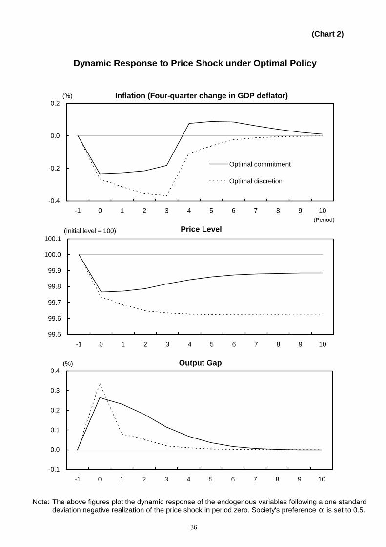
(Chart 2)

Note: The above figures plot the dynamic response of the endogenous variables following a one standarddeviation negative realization of the price shock in period zero. Society's preference α is set to 0.5.

Dynamic Response to Price Shock under Optimal Policy

-0.1

0.0

0.1

0.2

0.3

0.4

-1 0 1 2 3 4 5 6 7 8 9 10

(%)

-0.4

-0.2

0.0

0.2

-1 0 1 2 3 4 5 6 7 8 9 10

Optimal commitment

Optimal discretion

(%)

99.5

99.6

99.7

99.8

99.9

100.0

100.1

-1 0 1 2 3 4 5 6 7 8 9 10

(Initial level = 100)

Inflation (Four-quarter change in GDP deflator)

Output Gap

Price Level(Period)

36

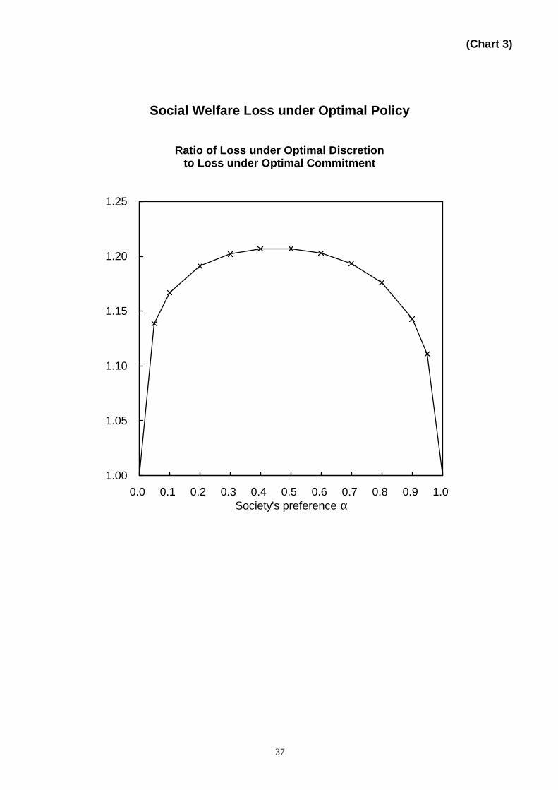
(Chart 3)

Social Welfare Loss under Optimal Policy

Ratio of Loss under Optimal Discretionto Loss under Optimal Commitment

1.00

1.05

1.10

1.15

1.20

1.25

0.0 0.1 0.2 0.3 0.4 0.5 0.6 0.7 0.8 0.9 1.0Society's preference α

37

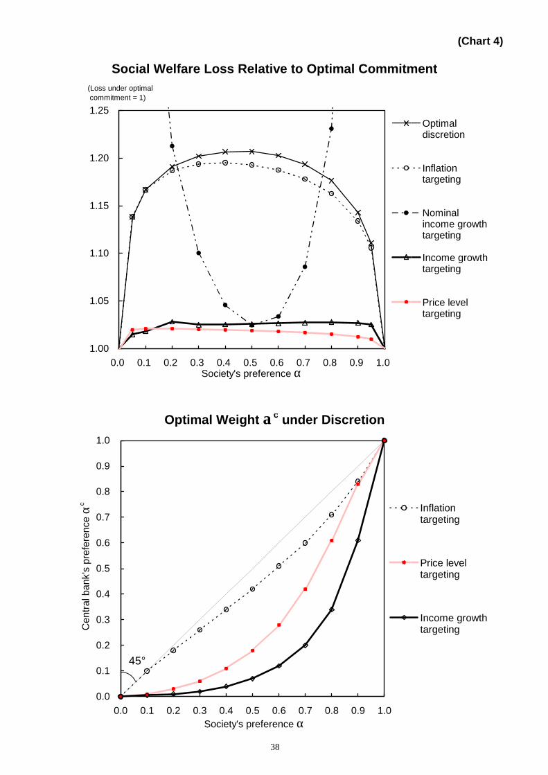
(Chart 4)

Optimal Weight αc under Discretion

Social Welfare Loss Relative to Optimal Commitment

0.0

0.1

0.2

0.3

0.4

0.5

0.6

0.7

0.8

0.9

1.0

0.0 0.1 0.2 0.3 0.4 0.5 0.6 0.7 0.8 0.9 1.0Society's preference α

Cen

tral b

ank'

s pr

efer

ence

αc Inflation

targeting

Price leveltargeting

Income growthtargeting

45°

1.00

1.05

1.10

1.15

1.20

1.25

0.0 0.1 0.2 0.3 0.4 0.5 0.6 0.7 0.8 0.9 1.0Society's preference α

Optimaldiscretion

Inflationtargeting

Nominalincome growthtargeting

Income growthtargeting

Price leveltargeting

(Loss under optimal commitment = 1)

38

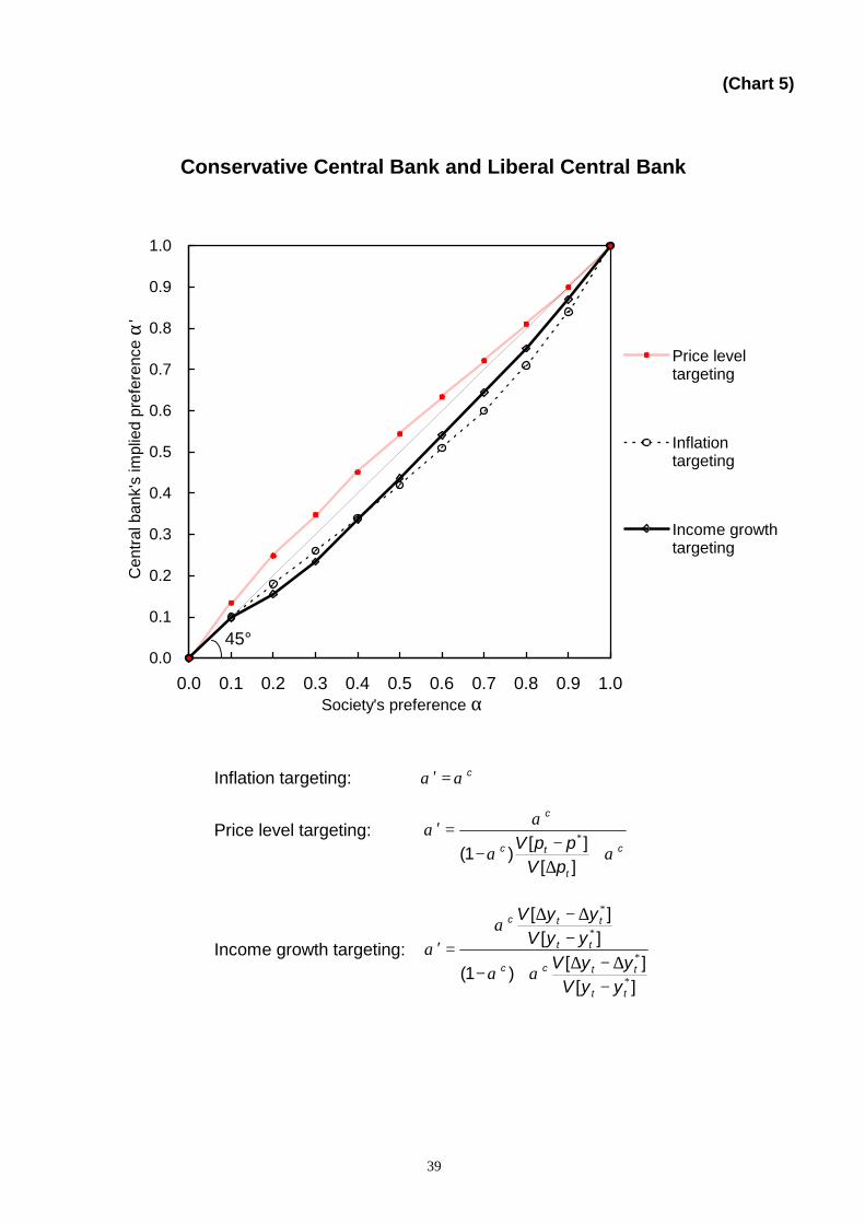
(Chart 5)

Conservative Central Bank and Liberal Central Bank

0.0

0.1

0.2

0.3

0.4

0.5

0.6

0.7

0.8

0.9

1.0

0.0 0.1 0.2 0.3 0.4 0.5 0.6 0.7 0.8 0.9 1.0Society's preference α

Cen

tral b

ank'

s im

plie

d pr

efer

ence

α'

Price leveltargeting

Inflationtargeting

Income growthtargeting

45°

Inflation targeting: cαα =′

Price level targeting:c

t

tc

c

pVppV αα

αα+

∆−−

=′ ∗

][][)1(

Income growth targeting:

][][)1(

][][

∗

∗

∗

∗

−∆−∆+−

−∆−∆

=′

tt

ttcc

tt

ttc

yyVyyV

yyVyyV

αα

αα

39

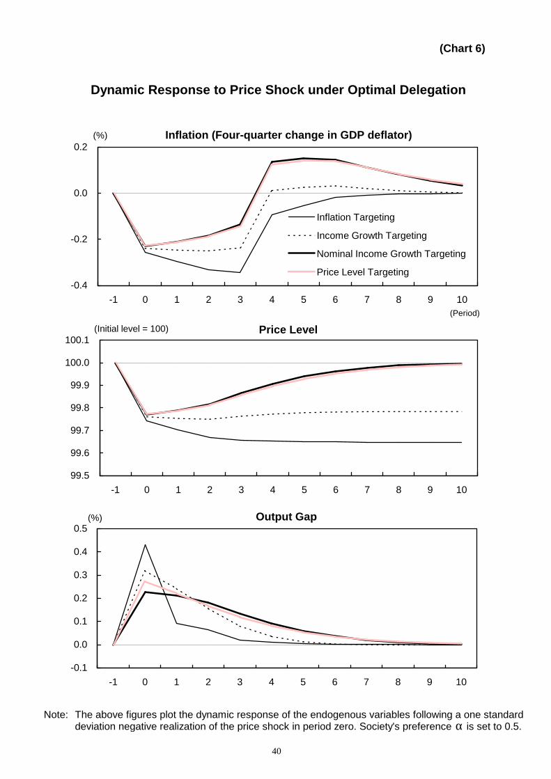
(Chart 6)

Note: The above figures plot the dynamic response of the endogenous variables following a one standarddeviation negative realization of the price shock in period zero. Society's preference α is set to 0.5.

Dynamic Response to Price Shock under Optimal Delegation

Inflation

-0.1

0.0

0.1

0.2

0.3

0.4

0.5

-1 0 1 2 3 4 5 6 7 8 9 10

(%)

-0.4

-0.2

0.0

0.2

-1 0 1 2 3 4 5 6 7 8 9 10

Inflation Targeting

Income Growth Targeting

Nominal Income Growth Targeting

Price Level Targeting

(%)

99.5

99.6

99.7

99.8

99.9

100.0

100.1

-1 0 1 2 3 4 5 6 7 8 9 10

(Initial level = 100)

Inflation (Four-quarter change in GDP deflator)

Output Gap

Price Level(Period)

40

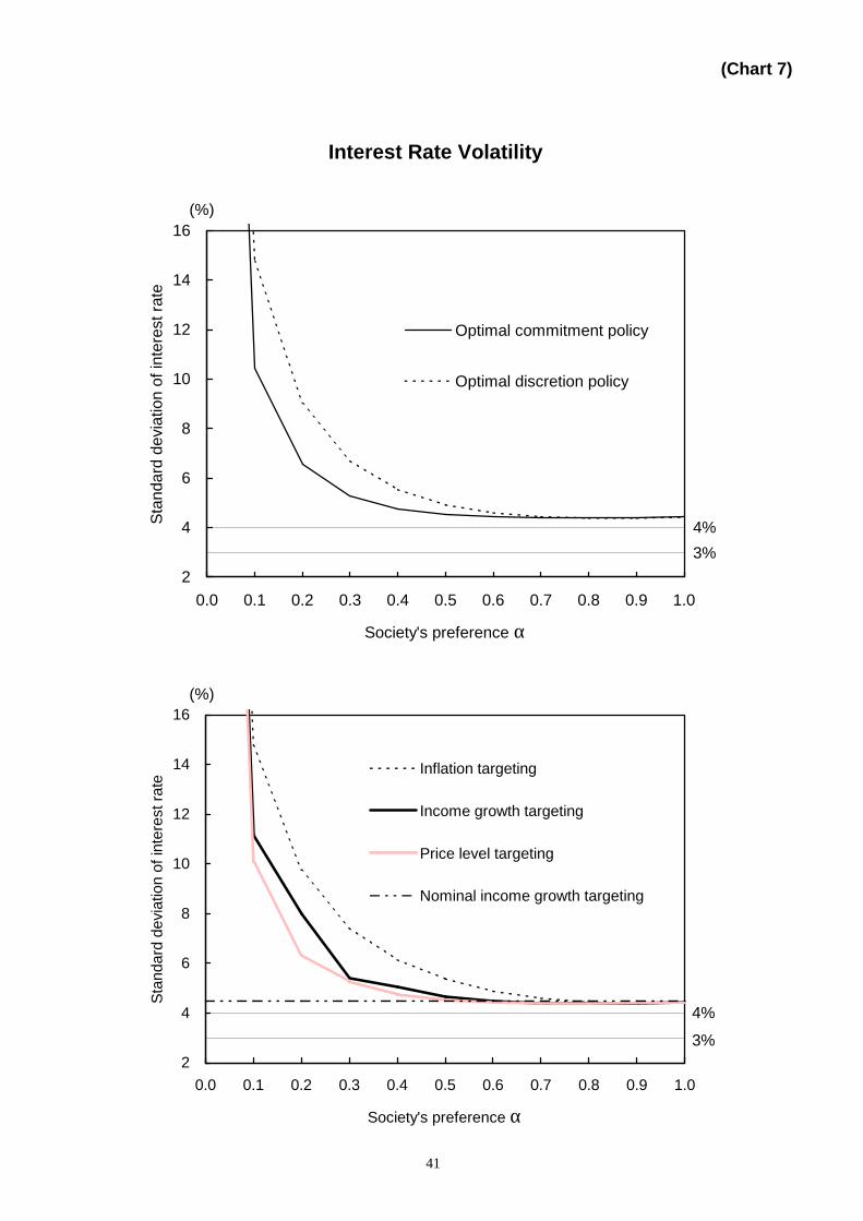
(Chart 7)

Interest Rate Volatility

2

4

6

8

10

12

14

16

0.0 0.1 0.2 0.3 0.4 0.5 0.6 0.7 0.8 0.9 1.0

Society's preference α

Sta

ndar

d de

viat

ion

of in

tere

st ra

te

Optimal commitment policy

Optimal discretion policy

4%

3%

(%)

2

4

6

8

10

12

14

16

0.0 0.1 0.2 0.3 0.4 0.5 0.6 0.7 0.8 0.9 1.0

Society's preference α

Sta

ndar

d de

viat

ion

of in

tere

st ra

te

Inflation targeting

Income growth targeting

Price level targeting

Nominal income growth targeting

4%

3%

(%)

41

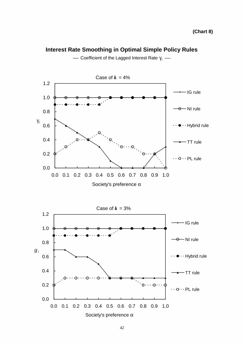
(Chart 8)

Interest Rate Smoothing in Optimal Simple Policy Rules Coefficient of the Lagged Interest Rate γi

0.0

0.2

0.4

0.6

0.8

1.0

1.2

0.0 0.1 0.2 0.3 0.4 0.5 0.6 0.7 0.8 0.9 1.0

Society's preference α

IG rule

NI rule

Hybrid rule

TT rule

PL rule

γi

Case of k = 4%

0.0

0.2

0.4

0.6

0.8

1.0

1.2

0.0 0.1 0.2 0.3 0.4 0.5 0.6 0.7 0.8 0.9 1.0

Society's preference α

IG rule

NI rule

Hybrid rule

TT rule

PL rule

γi

Case of k = 3%

42

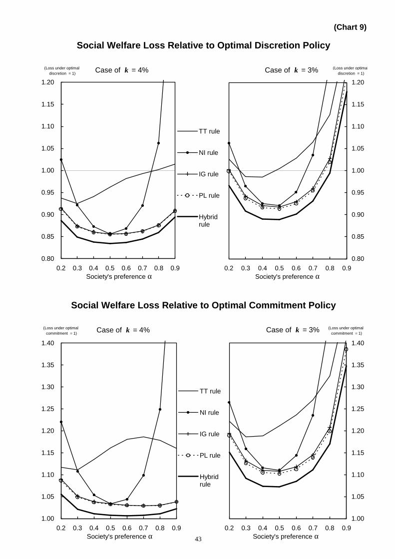
(Chart 9)

Social Welfare Loss Relative to Optimal Discretion Policy

Social Welfare Loss Relative to Optimal Commitment Policy

0.2 0.3 0.4 0.5 0.6 0.7 0.8 0.9Society's preference α

0.80

0.85

0.90

0.95

1.00

1.05

1.10

1.15

1.20

(Loss under optimal discretion = 1)Case of k = 3%

0.80

0.85

0.90

0.95

1.00

1.05

1.10

1.15

1.20

0.2 0.3 0.4 0.5 0.6 0.7 0.8 0.9Society's preference α

TT rule

NI rule

IG rule

PL rule

Hybridrule

(Loss under optimal discretion = 1) Case of k = 4%

1.00

1.05

1.10

1.15

1.20

1.25

1.30

1.35

1.40

0.2 0.3 0.4 0.5 0.6 0.7 0.8 0.9Society's preference α

TT rule

NI rule

IG rule

PL rule

Hybridrule

(Loss under optimal commitment = 1) Case of k = 4%

0.2 0.3 0.4 0.5 0.6 0.7 0.8 0.9Society's preference α

1.00

1.05

1.10

1.15

1.20

1.25

1.30

1.35

1.40

(Loss under optimal commitment = 1)Case of k = 3%

43

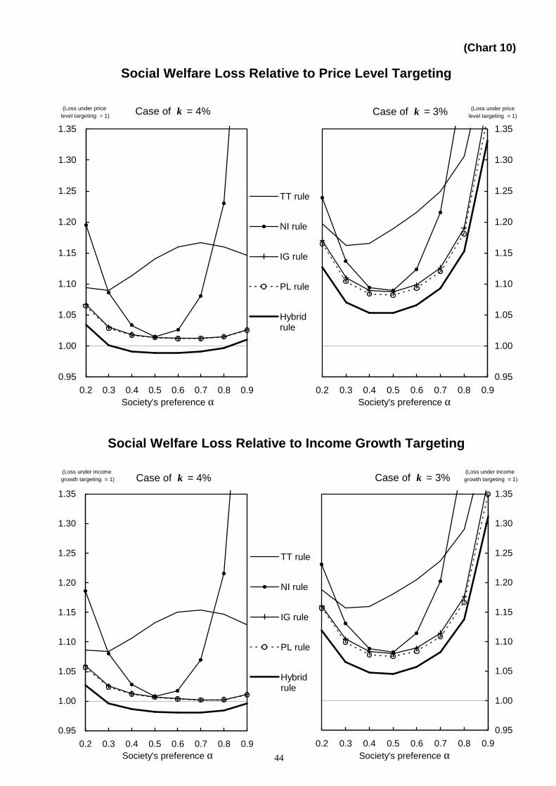
(Chart 10)

Social Welfare Loss Relative to Price Level Targeting

Social Welfare Loss Relative to Income Growth Targeting

0.2 0.3 0.4 0.5 0.6 0.7 0.8 0.9Society's preference α

0.95

1.00

1.05

1.10

1.15

1.20

1.25

1.30

1.35

(Loss under pricelevel targeting = 1)Case of k = 3%

0.95

1.00

1.05

1.10

1.15

1.20

1.25

1.30

1.35

0.2 0.3 0.4 0.5 0.6 0.7 0.8 0.9Society's preference α

TT rule

NI rule

IG rule

PL rule

Hybridrule

(Loss under price level targeting = 1) Case of k = 4%

0.95

1.00

1.05

1.10

1.15

1.20

1.25

1.30

1.35

0.2 0.3 0.4 0.5 0.6 0.7 0.8 0.9Society's preference α

TT rule

NI rule

IG rule

PL rule

Hybridrule

(Loss under income growth targeting = 1) Case of k = 4%

0.2 0.3 0.4 0.5 0.6 0.7 0.8 0.9Society's preference α

0.95

1.00

1.05

1.10

1.15

1.20

1.25

1.30

1.35

(Loss under income growth targeting = 1)Case of k = 3%

44

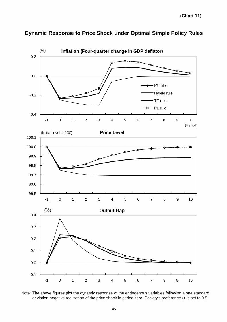
(Chart 11)

Note: The above figures plot the dynamic response of the endogenous variables following a one standarddeviation negative realization of the price shock in period zero. Society's preference α is set to 0.5.

Dynamic Response to Price Shock under Optimal Simple Policy Rules

(2) Inflation

-0.1

0.0

0.1

0.2

0.3

0.4

-1 0 1 2 3 4 5 6 7 8 9 10

(%)

-0.4

-0.2

0.0

0.2

-1 0 1 2 3 4 5 6 7 8 9 10

IG rule

Hybrid rule

TT rule

PL rule

(%)

99.5

99.6

99.7

99.8

99.9

100.0

100.1

-1 0 1 2 3 4 5 6 7 8 9 10

(Initial level = 100)

Inflation (Four-quarter change in GDP deflator)

Output Gap

Price Level

(Period)

45

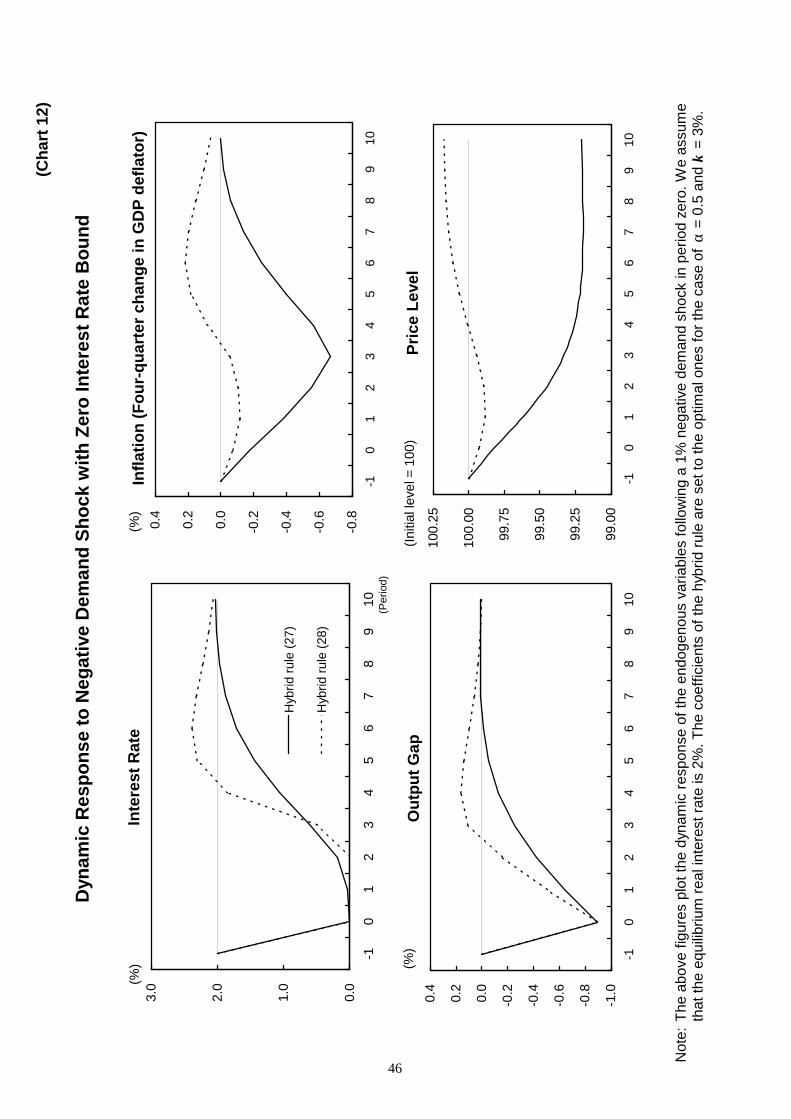
(Cha

rt 1

2)

N

ote:

The

abov

e fig

ures

plo

t the

dyn

amic

resp

onse

of t

he e

ndog

enou

s va

riabl

es fo

llow

ing

a 1%

neg

ativ

e de

man

d sh

ock

in p

erio

d ze

ro. W

e as

sum

eth

at th

e eq

uilib

rium

real

inte

rest

rate

is 2

%. T

he c

oeffi

cien

ts o

f the

hyb

rid ru

le a

re s

et to

the

optim

al o

nes

for t

he c

ase

of α

= 0

.5 a

nd k

= 3

%.

Dyn

amic

Res

pons

e to

Neg

ativ

e D

eman

d S

hock

with

Zer

o In

tere

st R

ate

Bou

nd

-1.0

-0.8

-0.6

-0.4

-0.20.0

0.2

0.4

-10

12

34

56

78

910

(%)

-0.8

-0.6

-0.4

-0.20.0

0.2

0.4

-10

12

34

56

78

910

(%)

99.0

0

99.2

5

99.5

0

99.7

5

100.

00

100.

25

-10

12

34

56

78

910

(Initi

al le

vel =

100

)

0.0

1.0

2.0

3.0

-10

12

34

56

78

910

Hyb

rid ru

le (2

7)

Hyb

rid ru

le (2

8)

(%)

Inte

rest

Rat

eIn

flatio

n (F

our-

quar

ter

chan

ge in

GD

P d

efla

tor)

Out

put G

apP

rice

Lev

el

(Per

iod)

46

47

Appendix

A. Numerical Solutions of Unique Rational Expectations Equilibrium underOptimal Commitment Policy and Optimal Simple Policy Rules

Consider the following linear rational expectations model:

+

=

×

+

+

+

1

1

1

1

0][ fn

t

ft

bt

ftt

bt

e

zz

MzE

z , (A1)

where btz denotes a ( 1×bn )-vector of predetermined (backward-looking) variables with their

initial values bz0 given, f

tz a ( 1×fn )-vector of non-predetermined (forward-looking)variables, and te a ( 1×bn )-vector of mean-zero innovations to

btz with covariance matrix Σ .

M is a )()( fbfb nnnn +×+ -matrix whose elements depend on the monetary policy

parameters (i.e. parameters on the first-order conditions or simple policy rules) as well asthe structural parameters of the economy.

We compute a unique stationary rational expectations equilibrium of the model (A1) byusing the Blanchard-Kahn method1. The reduced form representation of equilibriumprocesses is given by

btf

ft zMz = , 11 ++ += t

btb

bt ezMz . (A2)

The elements of the matrices fM and bM depend on those of matrix M .

We then conduct stochastic simulations of the reduced model (A2) to obtain thestochastic distributions of endogenous variables. Using the covariance matrix Σ ofinnovation te , we generate 100 sets of artificial normally-distributed shocks with 1,000

quarters of shocks in each set. We use these shocks to conduct stochastic simulations underalternative monetary policies, and calculate the variances of the endogenous variables (andthus the social welfare losses).

We can apply the above calculation method to solving a unique rational expectationsequilibrium under the optimal commitment policy and simple policy rules.

Case 1: Optimal Commitment Policy

Necessary for calculating a unique rational expectations equilibrium under the optimalcommitment policy are the following three equations:

ttttttt yypEpp µλθθ +−+∆−+∆=∆ ∗+− )(][)1( 11 , (2)

11 ˆ ++ += ttt µρµµ , (4)]}[))(1({)1( 1111

∗++

∗−−

∗ −−−−−−−=∆− tttttttt yyEyyyyp θθααλ , (7b)

1 See Blanchard and Kahn (1980), Söderlind (1999), and Klein (2000) for details of computationmethod.

48

where 011 =− ∗−− yy . (7a)

These equations can be reduced to the state-space form (A1), where

−∆=

∗−−

−

11

1

tt

t

tbt

yypzµ

,

=

00

0̂

0

µbz ,

−∆

= ∗tt

tft yy

pz ,

=

00

t̂

teµ

,

−−−−−−−−−−

=

θαθαλθθθλθθθθ

ρ

1)1()1(00)1()1(10)1()1(1

10000010000000

M .

Using the reduced form (A2) based on this state-space form, we calculate a unique rationalexpectations equilibrium to obtain unique optimal plans of the forward-looking variables,i.e. inflation and the output gap. Then, the interest rate implied by the IS curve (1) isdetermined, conditional on the unique optimal plans of inflation and the output gap.

Case 2: TT Rule

Necessary for calculating a unique rational expectations equilibrium under the TT rule are

the following six equations.

ttttttttttttt yEpEiyyEyyyy εσσφφ +∆−∆−−−−+−=− ∗+

−+

∗++

∗−−

∗ ])}[][(][){1()( 11

11111 , (1)

ttttttt yypEpp µλθθ +−+∆−+∆=∆ ∗+− )(][)1( 11 , (2)

11 ˆ++ += ttt εψ εε , (3)

11 ˆ ++ += ttt µρµµ , (4)

11ˆ)1( +

∗∗+ +∆+−=∆ ttt yy ξωτω , (5)

)(][)1( 11

1∗∗

+−

− −+∆+∆−+= ttytpttitit yypyEii γγσγγ . (17)

Note that, unlike the optimal commitment policy, the central bank cannot offset the effectsof the demand and productivity shocks on the economy completely when it adopts a simplepolicy rule which involves no explicit dependence on these shocks. Therefore, to calculatethe equilibrium process for endogenous variables under the TT rule, we must includeequations (1), (3), and (5) as well as (2) and (4) in the model.

The six equations above are written in state-space form (A1), where

−−

∆−∆

=

−

∗−−

−

∗

στ

τµε

1

11

1

t

tt

t

t

t

t

bt

iyy

py

z ,

=

00 0 0

ˆˆˆ

0

0

0

0

ξµε

bz ,

−∆

= ∗tt

tft yy

pz ,

=

000

ˆˆˆ

t

t

t

teξµε

,

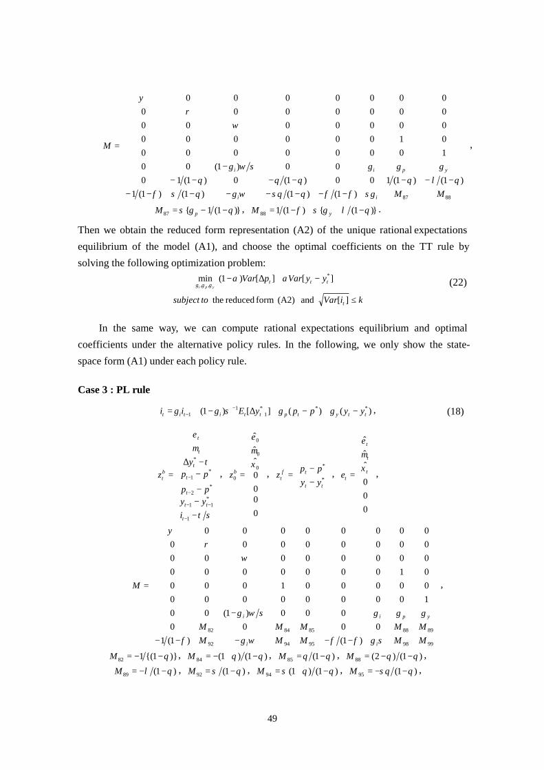
49

−−−−−−−−−−−−−−−

−

=

8887)1()1()1()1(1)1()1(100)1(0)1(10

00)1(001000000001000000000000000000000000000

MM

M

ii

ypii

σγφφθσθωγθσφθλθθθθ

γγγσωγ

ωρ

ψ

,

})1(1{87 θγσ −−= pM , })1({)1(188 θλγσφ −++−= yM .

Then we obtain the reduced form representation (A2) of the unique rational expectationsequilibrium of the model (A1), and choose the optimal coefficients on the TT rule bysolving the following optimization problem:

kiVartosubject

yyVarpVar

t

tttypi

≤

−+∆−

][ and (A2) form reduced the

][][)1( min *

,,αα

γγγ (22)

In the same way, we can compute rational expectations equilibrium and optimalcoefficients under the alternative policy rules. In the following, we only show the state-space form (A1) under each policy rule.

Case 3 : PL rule

)()(][)1( *1

11 ttytpttitit yyppyEii −+−+∆−+= ∗∗

+−

− γγσγγ , (18)

−−−−−∆

=

−

∗−−

∗−

∗−

∗

στ

τµε

1

11

2

1

t

tt

t

t

t

t

t

bt

iyypp

ppy

z ,

=

0000ˆˆˆ

0

0

0

0

ξµε

bz ,

−−= ∗

∗

tt

tft yy

ppz ,

=

000

ˆˆˆ

t

t

t

teξµε

,

−−−−−

−

=

9998959492

8988858482

)1()1(10000

000)1(00100000000000001000010000000000000000000000000000000

MMMMMMMMMM

M

ii

ypii

σγφφωγφ

γγγσωγ

ωρ

ψ

,

)}1{(182 θ−−=M , )1()1(84 θθ −+−=M , )1(85 θθ −=M , )1()2(88 θθ −−=M ,)1(89 θλ −−=M , )1(92 θσ −=M , )1()1(94 θθσ −+=M , )1(95 θσθ −−=M ,

50

})1(1{98 θγσ −−= pM , ])1([)1(199 θλγσφ −++−= yM .

Case 4 : IG rule and NI rule

)(][)1( *1

11 ttytpttitit yypyEii ∆−∆+∆+∆−+= ∗

+−

− γγσγγ , (19)

][][)1( *1

11 tttpttitit yypyEii ∆−∆+∆+∆−+= ∗

+−

− γσγγ , (20)

−−

∆−∆

=

−

∗−−

−

∗

στ

τµε

1

11

1

t

tt

t

t

t

t

bt

iyy

py

z ,

=

000

ˆˆˆ

0

0

0

0

ξµε

bz ,

−∆

= ∗tt

tft yy

pz ,

=

000

ˆˆˆ

t

t

t

teξµε

,

−−−−−−−−−−−−

−−

=

888785)1()1()1(1)1()1(100)1(0)1(10

0)1(001000000001000000000000000000000000000

MMM

M

ii

ypiyi

σγθσθωγθσφθλθθθθ

γγγγσωγ

ωρ

ψ

,

))1((85 yM σγφφ +−−= , })1(1{87 θγσ −−= pM , })1({)1(188 θλγσφ −++−= yM .

When we impose yp γγ = on the elements of matrix M, the state-space form (A1)

corresponds to the NI rule.

Case 5 : Hybrid rule

)()(][)1( *11

*1

11 −−

∗+

−− −+−+∆+∆−+= ttlyttytpttitit yyyypyEii γγγσγγ , (21)

−−

∆−∆

=

−

∗−−

−

∗

στ

τµε

1

11

1

t

tt

t

t

t

t

bt

iyy

py

z ,

=

000

ˆˆˆ

0

0

0

0

ξµε

bz ,

−∆

= ∗tt

tft yy

pz ,

=

000

ˆˆˆ

t

t

t

teξµε

,

−−−−−−−−−−−−

−

=

888785)1()1()1(1)1()1(100)1(0)1(10

0)1(001000000001000000000000000000000000000

MMM

M

ii

ypilyi

σγθσθωγθσφθλθθθθ

γγγγσωγ

ωρ

ψ

,

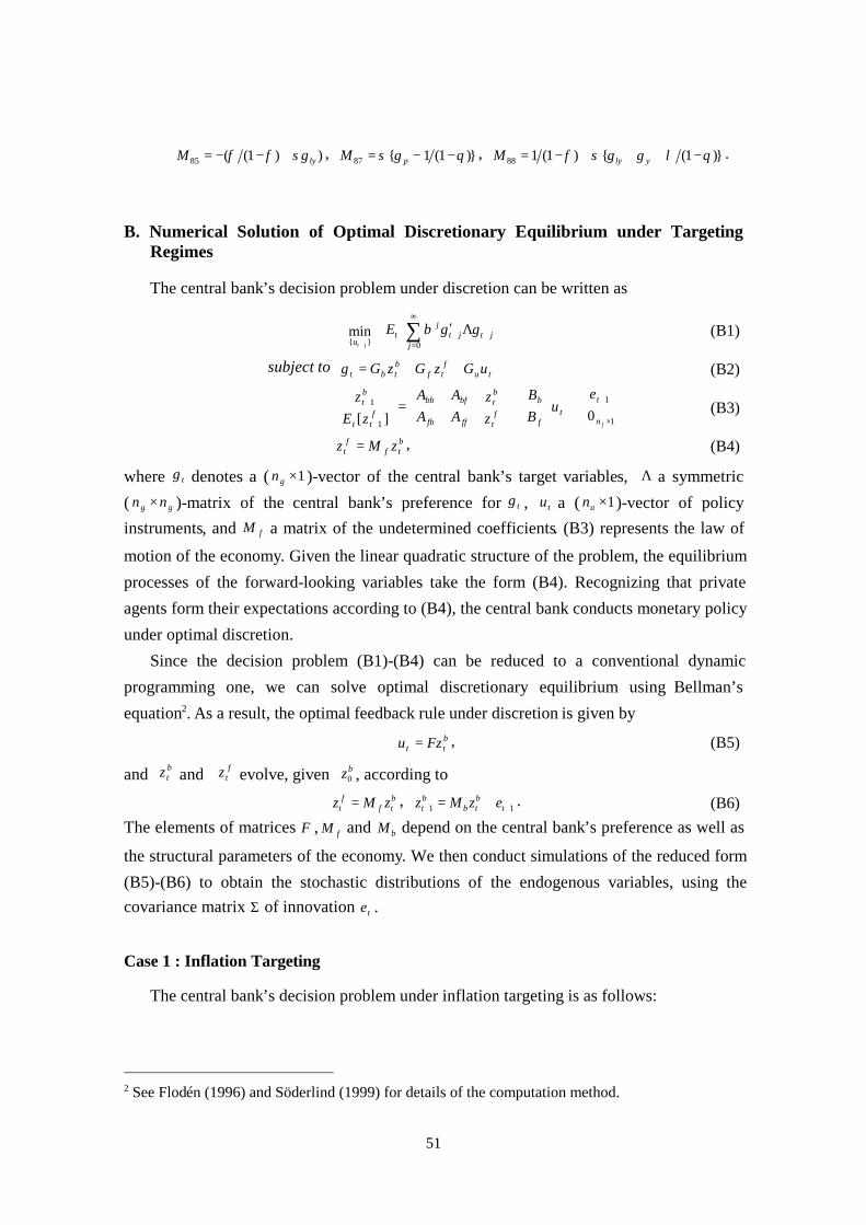
51

))1((85 lyM σγφφ +−−= , })1(1{87 θγσ −−= pM , })1({)1(188 θλγγσφ −+++−= ylyM .

B. Numerical Solution of Optimal Discretionary Equilibrium under TargetingRegimes

The central bank’s decision problem under discretion can be written as

Λ′∑

∞

=++

+ 0}{min

jjtjt

jt

uggE

jt

β (B1)

subject to tuf

tfbtbt uGzGzGg ++= (B2)

+

+

=

×

+

+

+

1

1

1

1

0][ fn

tt

f

bf

t

bt

fffb

bfbbf

tt

bt

eu

BB

zz

AAAA

zEz

(B3)

btf

ft zMz = , (B4)

where tg denotes a ( 1×gn )-vector of the central bank’s target variables, Λ a symmetric( gg nn × )-matrix of the central bank’s preference for tg , tu a ( 1×un )-vector of policyinstruments, and fM a matrix of the undetermined coefficients. (B3) represents the law of

motion of the economy. Given the linear quadratic structure of the problem, the equilibriumprocesses of the forward-looking variables take the form (B4). Recognizing that privateagents form their expectations according to (B4), the central bank conducts monetary policyunder optimal discretion.

Since the decision problem (B1)-(B4) can be reduced to a conventional dynamicprogramming one, we can solve optimal discretionary equilibrium using Bellman’sequation2. As a result, the optimal feedback rule under discretion is given by

btt Fzu = , (B5)

and btz and f

tz evolve, given bz0 , according tobtf

ft zMz = , 11 ++ += t

btb

bt ezMz . (B6)

The elements of matrices F , fM and bM depend on the central bank’s preference as well as

the structural parameters of the economy. We then conduct simulations of the reduced form(B5)-(B6) to obtain the stochastic distributions of the endogenous variables, using thecovariance matrix Σ of innovation te .

Case 1 : Inflation Targeting

The central bank’s decision problem under inflation targeting is as follows:

2 See Flodén (1996) and Söderlind (1999) for details of the computation method.

52

−+∆−∑

∞

=

∗+++

− ∗++ 0

22

}{})())(1{(min

jjtjtcjtc

jt

yyyypE

jtjt

ααβ (12)

subject to ttttttt yypEpp µλθθ +−+∆−+∆=∆ ∗+− )(][)1( 11 (2)

11 ˆ ++ += ttt µρµµ (4)

This problem can be reduced to the state-space form (B1)-(B3), where

∆

=− 1t

tbt p

zµ ,

=

00̂

0

µbz , tf

t pz ∆= , ∗−= ttt yyu ,

=

0t̂

teµ ,

−

=Λc

c

αα0

01 ,

=

0000

bG ,

=01

fG ,

=10

uG ,

=

000ρ

bbA ,

=10

bfA ,

[ ])1()1(1 θθθ −−−−=fbA , )1(1 θ−=ffA ,

=00

bB , )1( θλ −−=fB .

Solving this dynamic programming problem, we obtain the following equilibrium processesfor inflation and the output gap:

1−∆+=∆ ttt pbap ππµ ,

1−∗ ∆+=− tytytt pbayy µ .

Given these equilibrium processes, it follows from the IS curve (2) that the equilibriumprocess for the interest rate is

ttytt

tttytt

aayy

yypbbrii

εφσµσρφσφφσσ

π

π

)}1({1)()()}1({

)()}1({1)(

11 −+++−−+−−−∆++=

∗−−

∗∗

.

Case 2 : Price Level Targeting

The central bank’s decision problem under price level targeting is as follows:

−+−−∑

∞

=

∗++

∗+

− ∗++ 0

22

}{])())(1[(min

jjtjtcjtc

jt

yyyyppE

jtjt

ααβ (13)

subject to ttttttt yypEpp µλθθ +−+∆−+∆=∆ ∗+− )(][)1( 11 (2)

11 ˆ ++ += ttt µρµµ (4)

This problem can be reduced to the state-space form (B1)-(B3), where

−−=

∗−

∗−

ppppz

t

t

tbt

2

1

µ,

=

00

0̂

0

µbz , ∗−= ppz t

ft , ∗−= ttt yyu ,

=

00

t̂

teµ

,

−

=Λc

c

αα0

01 ,

=

00

00

00

bG ,

=01

fG ,

=10

uG ,

=

01000000ρ

bbA ,

=

010

bfA ,

[ ])1()1()1()1(1 θθθθθ −−+−−−=fbA , )1()2( θθ −−=ffA ,

=

000

bB ,

)1( θλ −−=fB .

53

Solving this dynamic programming problem, we obtain the following equilibrium processesfor inflation and the output gap:

)()( 21∗

−∗

−∗ −+−+=− ppcppbapp tptptpt µ ,

)()( 21∗

−∗

−∗ −+−+=− ppcppbayy tytytytt µ .

Given these equilibrium processes, it follows from the IS curve (2) that the equilibriumprocess for the interest rate is

ttyptt

tttyptyptt

aayy

yyppccppbbrii

εφσµσρφσφφσσσ)}1({1)()()}1({

)()}1({1))(1())((

11

1

−+++−−+−−−−−++−++=

∗−−

∗∗−

∗∗

.

Case 3 : Income Growth Targeting

The central bank’s decision problem under income growth targeting is as follows:

∆−∆+∆−∑

∞

=

∗+++

− ∗++ 0

22

}{})())(1{(min

jjtjtcjtc

jt

yyyypE

jtjt

ααβ (14)

subject to ttttttt yypEpp µλθθ +−+∆−+∆=∆ ∗+− )(][)1( 11 (2)

11 ˆ ++ += ttt µρµµ (4)

This problem can be reduced to the state-space form (B1)-(B3), where

−∆=

∗−−

−

11

1

tt

t

tbt

yypzµ

,

=

00

0̂

0

µbz , t

ft pz ∆= , ∗−= ttt yyu ,

=

00

t̂

teµ

,

−−

−=Λ

cc

cc

c

αααα

α

00

001,

=

100000000

bG ,

=

001

fG ,

=

010

uG ,

=

00000000ρ

bbA ,

=

010

bfA , [ ]0)1()1(1 θθθ −−−−=fbA , )1(1 θ−=ffA ,

=

100

bB , )1( θλ −−=fB .

Solving this dynamic programming problem, we obtain the following equilibrium processesfor inflation and the output gap:

)( 111∗−−− −+∆+=∆ ttttt yycpbap πππµ ,

)( 111∗−−−

∗ −+∆+=− ttytytytt yycpbayy µ .

Given these equilibrium processes, it follows from the IS curve (2) that the equilibriumprocess for the interest rate is

ttytt

ttytytt

aayy

yyccpbbrii

εφσµσρφσφφσσσ

π

ππ

)}1({1)()()}1({

)]()}1({1[)(

11 −+++−−+−−−++∆++=

∗−−

∗∗

.

Case 4 : Nominal Income Growth Targeting

The central bank’s decision problem under nominal income growth targeting is as

54

follows:

∆−∆+∆∑

∞

=

∗+++

− ∗++ 0

2

}{)(min

jjtjtjt

jt

yyyypE

jtjt

β (15)

subject to ttttttt yypEpp µλθθ +−+∆−+∆=∆ ∗+− )(][)1( 11 (2)

11 ˆ ++ += ttt µρµµ (4)

This problem can be reduced to the state-space form (B1)-(B3), where

−∆=

∗−−

−

11

1

tt

t

tbt

yypzµ

,

=

00

0̂

0

µbz , t

ft pz ∆= , ∗−= ttt yyu ,

=

00

t̂

teµ

,

−−−−

=Λ1 1111 1 11 1

,

=

100000000

bG ,

=

001

fG ,

=

010

uG ,

=

00000000ρ

bbA ,

=

010

bfA ,

[ ]0)1()1(1 θθθ −−−−=fbA , )1(1 θ−=ffA ,

=

100

bB , )1( θλ −−=fB .

Solving this dynamic programming problem, we obtain the following equilibrium processesfor inflation and the output gap:

)( 111∗−−− −+∆+=∆ ttttt yycpbap πππµ ,

)( 111∗−−−

∗ −+∆+=− ttytytytt yycpbayy µ .

Given these equilibrium processes, it follows from the IS curve (2) that the equilibriumprocess for the interest rate is

ttytt

ttytytt

aayy

yyccpbbrii

εφσµσρφσφφσσσ

π

ππ

)}1({1)()()}1({

)]()}1({1[)(

11 −+++−−+−−−++∆++=

∗−−

∗∗

.

Reference

Blanchard, O.J. and C.M. Kahn, “The Solution of Linear Difference Equations under Rational

Expectations”, Econometrica 48, pp.1305-1311, 1980.

Flodén, M., “The Time Consistency Problem of Monetary Policy under Alternative Supply Side

Modeling”, mimeo, Stockholm School of Economics, 1996.

Klein, P., “Using the Generalized Schur Form to Solve a Multivariate Linear Rational Expectations

Mode”, Journal of Economic Dynamics and Control 24, pp.1405-23, 2000.

Söderlind, P., “Solution and Estimation of RE Macromodels with Optimal Policy”, European

Economic Review 43, pp.813-823, 1999.