· mental effects, etc. This report is one of six in a series which purpose is to fill that infor-mation gap, by enabling counties and municipalities to make compara-

---

-

G R O U N D W A T E R I S N O T as well protected as one mightimagine. It is affected by pollutants in the ground, byacidification and eutrophication. A rise or fall in the water tablecan cause harmful effects. Groundwater quality can beinterpreted and evaluated using the model criteria in this report.

The report is one of a series of six reports published by theSwedish Environmental Protection Agency under the headingE N V I R O N M E N TA L Q U A L I T Y C R I T E R I A . The reports areintended to be used by local and regional authorities, as well asother agencies, but also contain useful information for anyonewith responsibility for, and an interest in, good environmentalquality.

Reports available in English are:Report No.

• Lakes and Watercourses 5050• Coasts and Seas 5052• Contaminated Sites 5053

Abridged versions in English of all the six reports are availableon the Agency’s home page: www.environ.se (under the headlinelegislation/guidelines).

REPORT 5051

Groundwater

REPORT 5051

Environmental Quality Criteria

Groundwater

Environm

ental Quality C

riteria - Groundw

aterR

EP

OR

T 50

51

Groundwater

2

TO ORDER Swedish Environmetal Protection AgencyCustomer ServicesSE-106 48 Stockholm, Sweden

TELEPHONE +46 8 698 1200TELEFAX +46 8 698 1515

E-MAIL [email protected] http://www.environ.se

ISBN 91-620-5051-6ISSN 0282-7298

© 2000 Swedish Environmental Protection Agency

PRODUCTION ARALIADESIGN IdéoLuck AB

TRANSLATION Maxwell Arding, Arding Language Services ABPRINTED BY Lenanders, Kalmar1ST EDITION 700 copies

MILJÖMÄRKT

34

1

T R Y C K S A K

145

3

Contents

Foreword 5

Summary 7

Environmental Quality Criteria 9

Environmental Quality Criteria for Groundwater 15

Division into type areas 20

Nine geologicaly distinctive regions 21

Five groundwater environments 23

Type areas 26

Well depth 26

Alkalinity – risk of acidification 28

Nitrogen 35

Salt – chloride 40

Redox 47

Metals 51

Pesticides 59

Water table 64

Instructions for deviation test 69

Presentation of data 72

Appendixes 75

Glossary 139

4

Working GroupMost of the background material for “Environmen-tal Quality Criteria for Groundwater” was produ-ced by the “Project group for Environmental Quali-ty Criteria for groundwater” during the period June1994–April 1998.

Permanent members of the project group were:

Professor Kevin BishopDepartment of Environmental Assessment, Swe-dish University of Agricultural Sciences, Uppsala

Ulf von BrömssenProject Leader, Sustainable DevelopmentDepartment, Swedish Environmetal ProtectionAgency, Stockholm

Barbro DanielssonEnvironmental Department, Municipality ofKatrineholm

Anders GrimvallFaculty of Statistics, Data and Information Science,Swedish University of Agricultural Sciences,Uppsala

Professor Gunnar GustafsonFaculty of Geology, Chalmers University ofTechnology, Gothenburg

Professor Gunnar JacksDepartment of Land and Water Resources, RoyalInstitute of Technology, Stockholm

Jan JohanssonEnvironmental Protection Unit, ÖstergötlandCounty Administrative Board, Linköping

Jacob JohnsonSwedish Geological Survey, Uppsala

Krister LjungströmImplementation and Enforcement Department,Swedish Environmetal Protection Agency,Stockholm

Lena MaxeDepartment of Land and Water Resources,Royal Institute of Technology, Stockholm

Annika NilssonImplementation and Enforcement Department,Swedish Environmetal Protection Agency,Stockholm

Maria ReinholdsonSustainable Development Department, SwedishEPA, Stockholm

The following have also been involved in theproduction of background material during thecourse of the project:

Mats Aastrup, Swedish Geological Survey, Uppsala

Marie-Louise Bengtsson, Golder Grundteknik KB,Gothenburg

Lars Bergström, Faculty of Soil Science, SwedishUniversity of Agricultural Sciences, Uppsala

Jonas Gierup, Swedish Geological Survey, Uppsala

Karin Hanze, National Chemicals Inspectorate,Solna

Karin Holmgren, Faculty of Geology, ChalmersUniversity of Technology, Gothenburg

Anders Hult, National Food Administration,Uppsala

Jenny Kreuger, Faculty of Soil Science, SwedishUniversity of Agricultural Sciences, Uppsala

Lars Lövdahl, Faculty of Forest Ecology, SwedishUniversity of Agricultural Sciences, Umeå

Lars Rapp, Department of Environmental Assess-ment, Swedish University of Agricultural Sciences,Uppsala

Doris Rosling, National Food Administration,Uppsala

Helén Stejmar Eklund, Faculty of Geology,Chalmers University of Technology, Gothenburg

Bo Thunholm, Swedish Geological Survey, Uppsala

Malin Åkerblom, International Science Programs,Uppsala University

We would like to express our gratitude to the aboveparticipants for their committed approach to thisproject.

Ulf von Brömssen and Maria Reinholdson were

responsible for editing and arranging the material.

English translation: Maxwell Arding, ArdingLanguage Services AB

5

Based on favourable experience with“Environmental Criteria for Lakes andWatercourses”, the Swedish Environmen-tal Protection Agency decided in 1994 todevelop a more comprehensive system forevaluating a variety of ecoystems, underthe heading of “ENVIRONMENTAL QUALITY

CRITERIA”. This development work hasresulted in six separate reports on: theForest Landscape, the Agricultural land-scape, Groundwater, Lakes and Water-courses, Coasts and Seas, and Contami-nated Sites.

ENVIRONMENTAL QUALITY CRITERIA

provide a means of interpreting and evaluat-ing environmental data which is scientifi-cally based, yet easy to understand. Indica-tors and criteria are also being developed bymany other countries and internationalorganizations. The Swedish EnvironmentalProtection Agency has followed those deve-lopments, and has attempted to harmoniseits criteria with corresponding internationalapproaches.

The reports generated thus far are basedon current accumulated knowledge of envi-ronmental effects and their causes. But thatknowledge is constantly improving, and itwill be necessary to revise the reports fromtime to time. Such revisions and other deve-lopments may be followed on the Environ-mental Protection Agency's Internet website, www.environ.se. Concise versions ofthe reports are available there as well.

Development of the environmental qua-lity criteria has been carried out in co-opera-tion with colleges and universities. Various

national and regional agencies have beenrepresented in reference groups. The projectleaders at the Environmental ProtectionAgency have been: Rune Andersson, Agricul-tural landscapes; Ulf von Brömssen, Ground-water; Kjell Johansson, Lakes and Water-courses; Sif Johansson, Coasts and Seas;Marie Larsson and Thomas Nilsson, ForestLandscapes; and Fredrika Norman, Contami-nated Sites.

Project co-ordinators have been MarieLarsson (1995-97) and Thomas Nilsson(1998). Important decisions and the estab-lishment of project guidelines have been theresponsibility of a special steering com-mittee consisting of Erik Fellenius (Chair-man), Gunnar Bergvall, Taina Bäckström, KjellCarlsson, Rune Frisén, Kjell Grip, Lars-ÅkeLindahl, Lars Lindau, Anita Linell, Jan Ter-stad, Eva Thörnelöf and Eva Ölundh.

In April of 1998, public agencies, col-leges and universities, relevant organizationsand other interested parties were providedthe opportunity to review and commentupon preliminary drafts of the reports. Thatprocess resulted in many valuable sugges-tions, which have been incorporated intothe final versions to the fullest extent pos-sible. The Swedish Environmental Protec-tion Agency is solely responsible for thecontents of the reports, and wishes toexpress its sincere gratitude to all who parti-cipated in their production.

Stockholm, Sweden, December 2000Swedish Environmental Protection Agency

Foreword

6

7

Summary

This report on groundwater is one of a six-part series of reports published by the SwedishEnvironmental Protection Agency under thetitle “Environmental Quality Criteria”. Theother titles in the series are the Forest Land-scape, the Agricultural Landscape, Lakes andWatercourses, Coasts and Seas and ContaminatedSites.

The purpose of this report is to enablelocal and regional authorities and others tomake accurate assessments of environmentalquality on the basis of available data on thestate of the environment and thus obtain abetter basis for environmental planning andmanagement by objectives. Each report con-tains model criteria for a selection of para-meters corresponding to the objectives andthreats existing in the area dealt with by thereport. The assessment involves two aspects:(i) an appraisal of the effects that measuredconditions may have on the environment orour health; (ii) an appraisal of the extent towhich the recorded state deviates from a“reference value”. In most cases the referencevalue represents an estimate of a “natural”state. The results of both appraisals are ex-pressed on a scale of 1–5.

The report on groundwater focuses on themain environmental threats facing ground-water. A sharp increase in air pollution duringthe twentieth century has greatly reduced thecapacity of soil and hence groundwater to actas a buffer against acidification, lower pH andelevated concentrations of cadmium, zinc, leadand arsenic. Increased use by farmers of nitro-genous fertilisers, small-scale infiltration ofeffluent and deposition of airborne nitrogen

on soils already saturated with the elementhave given rise to elevated concentrations ofnitrogen in groundwater. Large-scale abstrac-tion of groundwater changes flow direction inaquifers. This may result in saltwater intru-sions and alter redox (reduction and oxidation)conditions, leading to elevated concentrationsof iron and manganese and altered forms ofsulphur and nitrogen compounds. Thesethreats to groundwater are reflected in theselection of parameters appraised in thisreport. These are: nitrogen, chloride, metals,acidification risk, risk of pesticide presence,changes in groundwater redox and deviationsfrom natural fluctuations in the water table.The assessment involves two aspects: (i) anappraisal of whether the recorded state of thegroundwater may have any negative effectson its use for drinking purposes or negativeeffects on the aquatic biota; (ii) an appraisalof the extent to which the recorded state de-viates from the reference value. The report ongroundwater also describes methods forassessing whether or not the groundwater inan area studied is exposed to impact from apoint source.

8

9

The vision of an ecologically sustainable society includes protection ofhuman health, preservation of biodiversity, conservation of valuable naturaland historical settings, an ecologically sustainable supply and efficient use ofenergy and other natural resources. In order to determine how well basicenvironmental quality objectives and more precise objectives are being met,it is necessary to continuously monitor and evaluate the state of theenvironment.

Environmental monitoring has been conducted for many years at both the national and regional levels. But, particularly at the regional level,assessments and evaluations of current conditions have been hindered by a lack of uniform and easily accessible data on baseline values, environ-mental effects, etc.

This report is one of six in a series which purpose is to fill that infor-mation gap, by enabling counties and municipalities to make compara-tively reliable assessments of environmental quality. The reports can thusbe used to provide a basis for environmental planning, and for the settingof local and regional environmental objectives.

The series bears the general heading of “ENVIRONMENTAL QUALITY

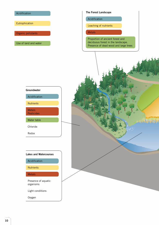
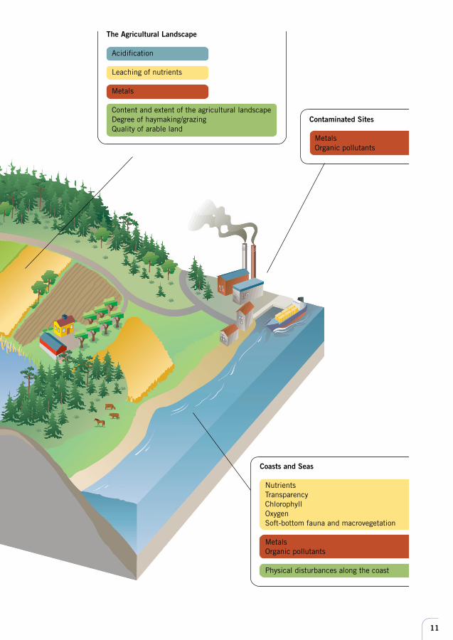
CRITERIA”, and includes the following titles: The Forest Landscape, TheAgricultural Landscape, Groundwater, Lakes and Watercourses, Coasts and Seas,and Contaminated Sites. Taken together, the six reports cover most of thenatural ecosystems and other types of environment found in Sweden. Itshould be noted, however, that coverage of wetlands, mountains andurban environments is incomplete.

Each of the reports includes assessment criteria for a selection of pa-rameters relating to objectives and threats that are associated with themain subject of the report. The selected parameters are, for the most part,the same as those used in connection with national and regional environ-mental monitoring programmes; but there are also some “new” parame-ters that are regarded as important in the assessment of environmentalquality.

Most of the parameters included in the series describe current condi-tions in natural environments, e.g. levels of pollution, while direct measuresof human impacts, such as the magnitude of emissions, are generally not


The vision of an ecologically sustainable society includes protection ofhuman health, preservation of biodiversity, conservation of valuable natu-ral and historical settings, an ecologically sustainable supply and efficient use of energy and other natural resources. In order to determine how wellbasic environmental quality objectives and more precise objectives arebeing met, it is necessary to continuously monitor and evaluate the state ofthe environment.

Environmental monitoring has been conducted for many years at both the national and regional levels. But, particularly at the regional level,assessments and evaluations of current conditions have been hindered by a lack of uniform and easily accessible data on baseline values, environ-mental effects, etc.

This report is one of six in a series which purpose is to fill that infor-mation gap, by enabling counties and municipalities to make compara-tively reliable assessments of environmental quality. The reports can thusbe used to provide a basis for environmental planning, and for the settingof local and regional environmental objectives.

The series bears the general heading of “ENVIRONMENTAL QUALITY

CRITERIA”, and includes the following titles: The Forest Landscape, The Agri-cultural Landscape, Groundwater, Lakes and Watercourses, Coasts and Seas, andContaminated Sites. Taken together, the six reports cover most of the naturalecosystems and other types of environment found in Sweden. It should benoted, however, that coverage of wetlands, mountains and urban environ-ments is incomplete.

Each of the reports includes assessment criteria for a selection of pa-rameters relating to objectives and threats that are associated with themain subject of the report. The selected parameters are, for the most part,the same as those used in connection with national and regional environ-mental monitoring programmes; but there are also some “new” parame-ters that are regarded as important in the assessment of environmentalquality.

Most of the parameters included in the series describe current condi-tions in natural environments, e.g. levels of pollution, while direct measuresof human impacts, such as the magnitude of emissions, are generally not

10

Lakes and Watercourses

Acidification

Nutrients

Metals

Presence of aquaticorganisms

Light conditions

Oxygen

Groundwater

Acidification

Nutrients

MetalsPesticides

Water table

Chloride

Redox

Acidification

Eutrophication

Organic pollutants

Use of land and water

The Forest Landscape

Acidification

Leaching of nutrients

Metals

Proportion of ancient forest anddeciduous forest in the landscape.Presence of dead wood and large trees

11

Coasts and Seas

NutrientsTransparencyChlorophyllOxygenSoft-bottom fauna and macrovegetation

MetalsOrganic pollutants

Physical disturbances along the coast

Contaminated Sites

MetalsOrganic pollutants

The Agricultural Landscape

Acidification

Leaching of nutrients

Metals

Content and extent of the agricultural landscapeDegree of haymaking/grazingQuality of arable land

12

included. In addition to a large number of chemical parameters, there areseveral that provide direct or indirect measures of biodiversity.

In all of the reports, assessments of environmental quality are handledin the same way for all of the parameters, and usually consist of two sepa-rate parts (see also page 13). One part focuses on the effects that observedconditions can be expected to have on environment and human health.Since knowledge of such effects is often limited, the solution in many caseshas been to present a preliminary classification scale based on generalknowledge about the high and low values that are known to occur in Swe-den.

The second focuses on the extent to which measured values deviatefrom established reference values. In most cases, the reference value repre-sents an approximation of a “natural” state, i.e. one that has been affectedvery little or not at all by human activities. Of course, “natural” is a conceptthat is not relevant to the preservation of cultural environments; in suchcontexts, reference values have a somewhat different meaning.

The results of both parts are expressed on a scale of 1-5, where Class 1indicates slight deviations from reference values or no environmentaleffects, and Class 5 indicates very large deviations or very significant effects.

The report on Contaminated Sites with its discussion of pollutants inheavily affected areas complements the other five reports. In those caseswhere the parameters are dealt with in several of the reports, which is par-ticularly the cases for metals, the report on Contaminated Sites corre-sponds (see further pages 13-14). However, the various parameters cannotbe compared with each other in terms of risks. The following paragraphsreview the extent of agreement with corresponding or similar systems usedby other countries and international organizations.

INTERNATIONAL SYSTEMS FOR ENVIRONMENTAL QUALITY ASSESSMENT

Among other countries, the assessment system that most resembles Swe-

den's is that of Norway. The Norwegian system includes “Classification of

Environmental Quality in Fjords and Coastal Waters” and “Environmental

Quality Classification of Fresh Water”. A five-level scale is used to classify

current conditions and usability. Classifications are in some cases based on

levels of pollution, in other cases on environmental effects.

The European Union's proposal for a framework directive on water quality

includes an assessment system that in many ways is similar to the Swedish

Environmental Quality Criteria.

If the parameters used in the latter are regarded as forms of environmental

indicators, there are many such systems in use or under development. How-

ever, the concept of environmental indicators is much broader than the

parameters of Environmental Quality Criteria.

13

Internationally, the most widely accepted framework for environmental indi-

cators is based on PSR-chains (Pressure-State-Response). Indicators are

chosen which reflect the relationship between environmental effects, and/or

there causes and measures taken. There is also a more sophisticated version,

called DPSIR (Driving forces-Pressure-State-Impact-Response). Variants of

the PSR/DPSIR systems are used by, among others, the OECD, the Nordic

Council of Ministers, the United Nations, the World Bank, the European

Union's Environmental Agency.

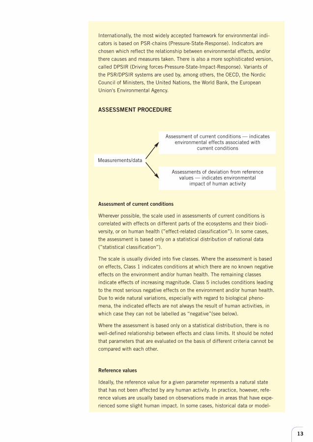
ASSESSMENT PROCEDURE

Assessment of current conditions

Wherever possible, the scale used in assessments of current conditions is

correlated with effects on different parts of the ecosystems and their biodi-

versity, or on human health (”effect-related classification”). In some cases,

the assessment is based only on a statistical distribution of national data

(”statistical classification”).

The scale is usually divided into five classes. Where the assessment is based

on effects, Class 1 indicates conditions at which there are no known negative

effects on the environment and/or human health. The remaining classes

indicate effects of increasing magnitude. Class 5 includes conditions leading

to the most serious negative effects on the environment and/or human health.

Due to wide natural variations, especially with regard to biological pheno-

mena, the indicated effects are not always the result of human activities, in

which case they can not be labelled as “negative”(see below).

Where the assessment is based only on a statistical distribution, there is no

well-defined relationship between effects and class limits. It should be noted

that parameters that are evaluated on the basis of different criteria cannot be

compared with each other.

Reference values

Ideally, the reference value for a given parameter represents a natural state

that has not been affected by any human activity. In practice, however, refe-

rence values are usually based on observations made in areas that have expe-

rienced some slight human impact. In some cases, historical data or model-

Assessment of current conditions — indicatesenvironmental effects associated with

current conditions

Assessments of deviation from referencevalues — indicates environmental

impact of human activity

Measurements/data

14

based estimates are used. Given that there are wide natural variations of

several of the parameters, reference values in many cases vary by region or

type of ecoystem.

Deviations from reference values

The extent of human impact can be estimated by calculating deviations from

reference values, which are usually stated as the quotient between a meas-

ured value and the corresponding reference value:

Measured valueDeviation = -------------------------------------

Reference value

The extent of deviation is usually classified on a five-level scale. Class 1

includes conditions with little or no deviation from the reference value, which

means that effects of human activity are negligible. The remaining classes

indicate increasing levels of deviation (increasing degree of impact). Class 5

usually indicates very significant impact from local sources.

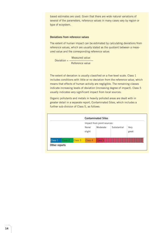
Organic pollutants and metals in heavily polluted areas are dealt with in

greater detail in a separate report, Contaminated Sites, which includes a

further sub-division of Class 5, as follows:

Contaminated Sites

Impact from point sources:

None/ Moderate Substantial Very

slight great

Class 1 Class 2 Class 3 Class 4 Class 5

Other reports

15

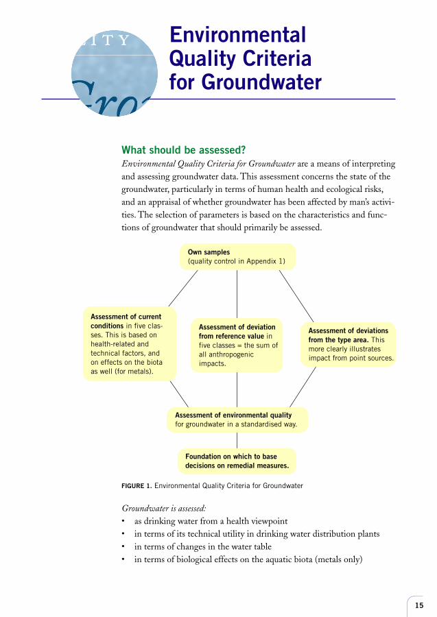
What should be assessed?Environmental Quality Criteria for Groundwater are a means of interpretingand assessing groundwater data. This assessment concerns the state of thegroundwater, particularly in terms of human health and ecological risks,and an appraisal of whether groundwater has been affected by man’s activi-ties. The selection of parameters is based on the characteristics and func-tions of groundwater that should primarily be assessed.

EnvironmentalQuality Criteriafor Groundwater

Groundwater is assessed:• as drinking water from a health viewpoint• in terms of its technical utility in drinking water distribution plants• in terms of changes in the water table• in terms of biological effects on the aquatic biota (metals only)

Own samples(quality control in Appendix 1)

Assessment of environmental qualityfor groundwater in a standardised way.

Foundation on which to basedecisions on remedial measures.

FIGURE 1. Environmental Quality Criteria for Groundwater

Assessment of currentconditions in five clas-ses. This is based onhealth-related andtechnical factors, andon effects on the biotaas well (for metals).

Assessment of deviationfrom reference value infive classes = the sum ofall anthropogenicimpacts.

Assessment of deviationsfrom the type area. Thismore clearly illustratesimpact from point sources.

16

All assessments relates to aquifers. Samples may be taken from ground-water pipes, springs or wells. Samples from pipe systems should be takenas close to the well as possible (see also Appendix 1).

Environmental state and threatsThe chemical composition of groundwater has changed on a large scale.The main threats are acidification and extensive leaching of nitrogen.Deposition of acidifying nitrogen and sulphur compounds result in fallingalkalinity and pH, increasing the mobility of metals in the soil. Otherimpacts result from agriculture and forestry, the transport sector, energygeneration, industry, the urban environment, quarries, mines and gravelpits. Excessive abstraction of groundwater may create a water shortage andcause changes in water quality, eg, increased salt or sulphate content.Private and municipal water supplies are sometimes contaminated in agri-cultural areas by nitrogen leaching out of the soil. A few studies haveshown that pesticides can also enter wells via groundwater. Contaminationfrom sewage causes microbial pollution of the groundwater and leachatefrom landfilled waste may have a wide range of effects on groundwater.Another threat is the large quantity of chemical products transported ashazardous goods. These goods are often transported through areas con-taining sensitive aquifers and catchment areas for drinking water supply.

Seven aspects are assessedGroundwater state is assessed on the basis of seven aspects:• alkalinity – risk of acidification• nitrogen• salt – chloride• redox• metals• pesticides• water table

The aspects dealt with only concern fairly extensive threats to groundwaterdue to human activities.

For regulations and assessment of drinking water quality, see the Na-tional Food Administration guidelines for drinking water quality and theEnvironmental Health Report.

For various reasons, the following aspects are not assessed in this re-port: radon, fluoride, phosphate, organic pollutants (except for pesticides)and pathogenic microorganisms.

Radon and fluoride are not included because the anthropogenic influen-ce on the concentrations of these substances is very limited and becauseelevated concentrations in aquifers cannot normally be remedied using

17

environmental protection techniques. Natural concentrations and healtheffects caused by these substances are presented in Appendix 9.

The occurrence of pathogenic microorganisms is largely of anthropogenicorigin. For assessment of current conditions, see the Drinking WaterRegulations issued by the National Food Administration.

Phosphate has been excluded since, being tightly fixed in soil, it usuallyoccurs in very low concentrations in groundwater. Moreover, there is nolimit value for health effects of phosphate.

As yet, we know little about organic pollutants in groundwater and thesesubstances (with the exception of pesticides) have therefore been omittedfrom the assessment. Exclusion of these substances may be reviewed whenthis report is revised.

ParametersEach aspect is described using reliable and well-established parameters.For recommended sampling and analysis methods, see the Swedish EPAEnvironmental Monitoring Handbook (in swedish only). In addition,Appendix 1 contains a brief description of the points in time when samp-les should be taken and of sampling and analytical methods. As manyparameters as possible should be included in the assessment so as to obtainas complete a picture of groundwater state as possible. There is nothing toprevent use of just a few parameters, however.

Division into type areasA set of type areas has been created to allow comparisons of similar typesof groundwater. Each type area is based on a combination of nine geologicalregions, five groundwater environments and two well-depth classes; see alsothe chapter entitled “Division into type areas”.

Assessment of current conditionsIn most cases, classification of state is based on the risk of health effectscaused by consumption of drinking water. In addition, there are technicaland aesthetic effects connected with use of the water as drinking water.The National Food Administration guide values and limit values (publicwater distribution plants) for drinking water quality are used in makingthese classifications. Concentrations at which effects begin to occur inaquatic biota in sensitive surface waters have been included as the basis forassessing metals. A five-point scale is used to assess water state. Class fiverepresents the greatest effects. The class boundaries indicating effects arepresented for each parameter. Other class boundaries have been set toprovide the greatest possible degree of accuracy at the most frequent con-centrations. Recorded levels coinciding with boundary between two classesare placed in the lower class.

18

Reference valuesThe basis for setting the reference value is described for each parameter.There are no reference values for “Alkalinity - risk of acidification”, “Re-dox” and “Water table”. In these cases only changes over time are assessed.The chapter on pesticides is presented as a risk classification of possibleoccurrence of pesticides in groundwater in the areas studied. Sampling andanalysis of samples should be given priority where the risk is greatest.

Assessment of deviation from reference valuesAssessment of deviation from the reference value is made in five classes.The boundary between class 1 and 2 constitutes the reference value. Hen-ce, class 1 covers the natural variation for the parameter. Levels of somemetals are naturally elevated above the reference value in small areas. The-se are described separately. The five classes encompass the national rangeof recorded values. The progression from class 2 to class 5 represents anincreasing degree of impact. Recorded levels coinciding with the boundarybetween two classes are placed in the lower class.

Assessment of whether a local point source is causingan impact – deviation testTo ascertain whether the data obtained from a type area is affected by apoint source, a comparison is made with the conditions in the referencepopulation for the type area using a deviation test. This will establishwhether or not the deviation is significant but will not provide any otherinformation. This assessment thus differs from the other two types of ass-essment: current conditions and deviation from reference value, which aremade in five classes.

The data population for a type area comprises all data in the referencedatabase from a groundwater environment in a geological region. The data,which date from the 1980s, has been cleaned up by eliminating valuescaused by obvious point source influence. It reflects the regional impact ofnatural factors (geology and climate) and non-point source anthropogenicimpact, such as land use and atmospheric deposition.

Comparisons with other reports in the seriesWhen comparing surface water and groundwater, it is important to bear inmind that they differ quite considerably in terms of the concentrations ofmany substances. In particular, ancient groundwater from great depths hashigher ionic strength than surface water. On the other hand, near-surfacegroundwater may be more acidic than almost all surface water and therefo-re have a high content of pH-sensitive metals like cadmium. This is onereason that the class boundaries for deviation from the reference value arehigher for groundwater than for surface water.

19

Far less medium-depth and deep groundwater with a long turnover timeenters the surface water than does near-surface groundwater with a shortturn-over time. Drinking water supplied from groundwater is normally ofmedium depth or deep groundwater, but the main contribution of ground-water to surface water consists of near-surface groundwater. This ground-water may due to acidification contain elevated levels of metals. This contri-bution of metals to surface water has been considered and metals in ground-water are classified according to judgements done in the report on lakes andwatercourses.

Because of the weak link between surface water flow and groundwater,it is difficult to determine the influence of groundwater on surface waterchemistry. The contribution from metals has been considered, however,whereas other constituents have been deemed to have little effect. The report on lakes and watercourses classifies nitrogen based on nitrogenleaching from soil, including flow via groundwater.

As regards deviation from the reference value, metals at very highconcentrations are further broken down in the report on contaminated sites.

Scale of applicationThis report is intended to be used primarily to assess the state of ground-water within an aquifer, municipality or county. Geological and hydrologicalconditions vary, both laterally and vertically, and groundwater quality, flowand level within an area therefore also vary. To make analysis of the chemicaldata easier, it is important to compare samples of groundwater that haveenvolved under similar conditions. To achieve this, each sampling point mustbe classified according to one of the 36 specified type areas and all ground-water conditions must be described by type area. (Where there is a largeamount of data, it is suggested that the type area be divided into two well-depth classes.)

Groundwater data varies not only in time, between sampling points, butalso over time. Sampling data must be representative of the type area towhich it relates. The smaller the sample, the greater the likelihood of obtain-ing an incorrect mean figure for concentrations in the type area studied. It isgenerally recommended that at least 25–30 sets of sampling data be used toassess a type area, see Appendix 1. A single sample taken on a single occasiononly represents itself and cannot be extrapolated to cover a larger area.

Quality assuranceAll analyses should be performed at accredited laboratories.

ReferencesStatutes of the National Food Administration 1993:35 and 1997:32.

Environmental Health Report (SOU 1996:124).

20

A division into type areas is presented here. Account has been taken of

factors, such as bedrock and soil types, having a bearing on the chemical

composition of groundwater. The division into type areas makes it easier to

understand various types of aquifer and is useful when comparing large

quantities of data with reference materials from the same type area. Areas

displaying anthropogenic impact from point sources can be identified using

a deviation test.

Having examined the groundwater in a given area, one often wishes toknow whether this water is similar to or, as a consequence of local impact,differs from other groundwater existing under similar conditions. A divi-sion into 36 type areas has been made to aid comparison of analyses. With-in a given type area, reasonably unaffected water will have similar concen-trations of the substances dealt with in this report. The type areas are basedon a combination of nine geological regions and five local groundwater envi-ronments. Shallow and deep wells are assessed separately in two well-depthclasses in each type area.

Table 1 shows the 36 type areas listed in Appendix 2. The appendixshows a breakdown by type area of concentrations of the substances co-vered in the report. There is also a breakdown according to well depth.Data has been obtained from a reference database at the Swedish Geologi-cal Survey based on nearly 30,000 wells, mainly analysed in the 1980s.These concentrations do not differ appreciably from present levels, exceptthat sulphur levels are now lower as a result of lower sulphur deposition.

The type areas are designed to achieve a minimal spread of data withineach population. The division into type areas has been based on the factorsof greatest importance in terms of the chemical composition of ground-water. Clear differences between the type areas are evident in relation toalkalinity, chloride and redox conditions, among others.

For the deviation test, see the chapter entitled “Instructions for deviationtest”, page 69. This method highlights areas affected by point sources andcan be used to supplement comparisons with reference values. The methodis well suited for use with large quantities of data.

Division into type areas

21

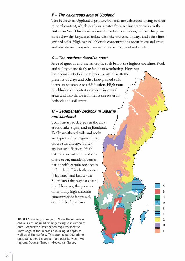
Nine geologically distinctive regionsIn order to identify different head groups of chemical composition of Swedishgroundwater, a correlation analysis has been performed on different causalpreconditions such as type of bedrock, type of hydrology, whether the presentland surface has been under seawater or not (the highest coastline). This hasresulted in a classification of the country in nine types of geological/geo-graphical regions (see Figure 2). This classification is based primarily on bed-rock type: (1) sedimentary rock (chalk, limestone, schists, sandstones) and (2)igneous rocks (granite, gneiss, granodiorite etc). A second factor is elevationin relation to the reference elevation, referred to in Sweden as “the highestcoastline”.

A – Sedimentary bedrock in southern SwedenSedimentary rock types in Skåne, and on the islands of Öland and Gotland.Easily weathered soils and rocks are typical of the region. These provide aneffective buffer against acidification. High natural concentrations of sulphatemay occur in the presence of certain rock types. Lies both below and abovethe highest coastline.

B – The highlands of southern SwedenAreas of igneous and metamorphic rock above the highest coastline fromSkåne to southern Närke. Rock and soil types are fairly resistant to weather-ing, which gives poor acidification buffering capacity. Western areas, in parti-cular, are exposed to high deposition of acidifying agents.

C – The west and south coastAreas of igneous and metamorphic rock below the highest coastline along thewest coast and east coast, and also the Kalmar Sound sandstone along thecoast of Småland. Here too, rock and soil types are fairly slow weathering.However, their position below the highest coastline and the presence of claysand other fine-grained soils increases resistance to acidification. High naturalchloride concentrations occur in coastal areas and also derive from relict seawater in bedrock and soil strata. There is high deposition of acidifying agents.

D – Sedimentary bedrock in central SwedenSedimentary bedrock in Västergötland, Östergötland and Närke. The regionmay be compared with region A.

E – The central Swedish depressionAreas of igneous and metamorphic rock below the highest coastline aroundthe large lakes of central Sweden. Rock and soil types fairly resistant toweathering. However, their position below the highest coastline and the pre-sence of clays and other fine-grained soils increases resistance to acidification.High natural chloride concentrations occur in coastal areas and also derivefrom relict sea water in bedrock and soil strata.

22

A

B

C

D

E

F

G

H

I

F – The calcareous area of UpplandThe bedrock in Uppland is primary but soils are calcareous owing to theirmineral content, which partly originates from sedimentary rocks in theBothnian Sea. This increases resistance to acidification, as does the posi-tion below the highest coastline with the presence of clays and other fine-grained soils. High natural chloride concentrations occur in coastal areasand also derive from relict sea water in bedrock and soil strata.

G – The northern Swedish coastArea of igneous and metamorphic rock below the highest coastline. Rockand soil types are fairly resistant to weathering. However,their position below the highest coastline with thepresence of clays and other fine-grained soilsincreases resistance to acidification. High natu-ral chloride concentrations occur in coastalareas and also derive from relict sea water inbedrock and soil strata.

H – Sedimentary bedrock in Dalarnaand JämtlandSedimentary rock types in the areaaround lake Siljan, and in Jämtland.Easily weathered soils and rocksare typical of the region. Theseprovide an effective bufferagainst acidification. Highnatural concentrations of sul-phate occur, mainly in combi-nation with certain rock typesin Jämtland. Lies both above( Jämtland) and below (theSiljan area) the highest coast-line. However, the presenceof naturally high chlorideconcentrations is unusual,even in the Siljan area.

FIGURE 2. Geological regions. Note: the mountainchain is not included (mainly owing to insufficientdata). Accurate classification requires specificknowledge of the bedrock occurring at depth aswell as at the surface. This applies particularly todeep wells bored close to the border between tworegions. Source: Swedish Geological Survey.

23

I – Igneous and metamorphic rock in inland northern Swedenabove the highest coastlineAreas of igneous and metamorphic rock above the highest coastline fromDalsland in the south-west to Treriksröset in the north. Rock and soiltypes are fairly resistant to weathering and therefore offer little resistanceto acidification. Low deposition. However, variations in natural conditionsoccur within this large area. For example, western Dalarna is unusual inhaving particularly slow-weathering bedrock in the form of Jotnian sand-stone and Dala porphyr, which provide poor buffering against acidifica-tion. Large areas of the far north are bog and peat land, which may createreducing conditions and high concentrations of iron and manganese in thegroundwater (see the chapter on “Redox”).

Five groundwater environmentsPrecipitation infiltrating the soil surface sinks through the unsaturatedzone to the saturated groundwater zone and then flows into the aquifer.The chemical composition of the groundwater is determined by thechemistry of the precipitation, the length of time the water is in contactwith organic and inorganic matter in the soil, the geochemical composi-tion of the soil and rock and the various strata sequences at the site.Ground conditions are therefore classified into five groundwater environ-ments to cover the differing strata sequences that cause the chemicalcharacteristics of the groundwater to vary (Bengtsson & Gustafson, 1996and Stejmar, 1996). These groundwater environments often form a mosaicin the landscape. The five groundwater environments are presented below.

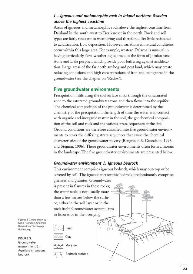
Groundwater environment 1: Igneous bedrockThis environment comprises igneous bedrock, which may outcrop or becovered by soil. The igneous metaorphic bedrock predominantly comprisesgneisses and granites. Groundwateris present in fissures in these rocks;the water table is not usually morethan a few metres below the surfa-ce, either in the soil layer or in therock itself. Groundwater accumulatesin fissures or in the overlying

FIGURE 3.Groundwaterenvironment 1:Aquifers in igneousbedrock syta

1.

Figures 3-7 were drawn byKarin Holmgren, ChalmersUniversity of Technology,Gothenburg Peat

Clay

Moraine

Bedrock surface

24

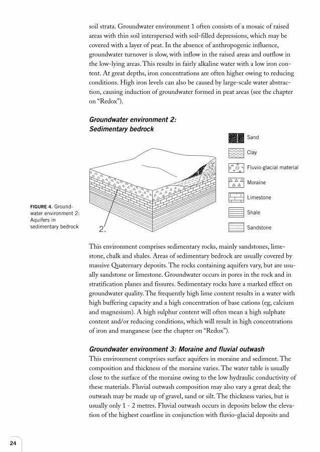
FIGURE 4. Ground-water environment 2:Aquifers insedimentary bedrock

Morän

Sand

Isälvsmaterial

Sandsten

Kalksten

Skiffer

Lera

2.

soil strata. Groundwater environment 1 often consists of a mosaic of raisedareas with thin soil interspersed with soil-filled depressions, which may becovered with a layer of peat. In the absence of anthropogenic influence,groundwater turnover is slow, with inflow in the raised areas and outflow inthe low-lying areas. This results in fairly alkaline water with a low iron con-tent. At great depths, iron concentrations are often higher owing to reducingconditions. High iron levels can also be caused by large-scale water abstrac-tion, causing induction of groundwater formed in peat areas (see the chapteron “Redox”).

Groundwater environment 2:Sedimentary bedrock

This environment comprises sedimentary rocks, mainly sandstones, lime-stone, chalk and shales. Areas of sedimentary bedrock are usually covered bymassive Quaternary deposits. The rocks containing aquifers vary, but are usu-ally sandstone or limestone. Groundwater occurs in pores in the rock and instratification planes and fissures. Sedimentary rocks have a marked effect ongroundwater quality. The frequently high lime content results in a water withhigh buffering capacity and a high concentration of base cations (eg, calciumand magnesium). A high sulphur content will often mean a high sulphatecontent and/or reducing conditions, which will result in high concentrationsof iron and manganese (see the chapter on “Redox”).

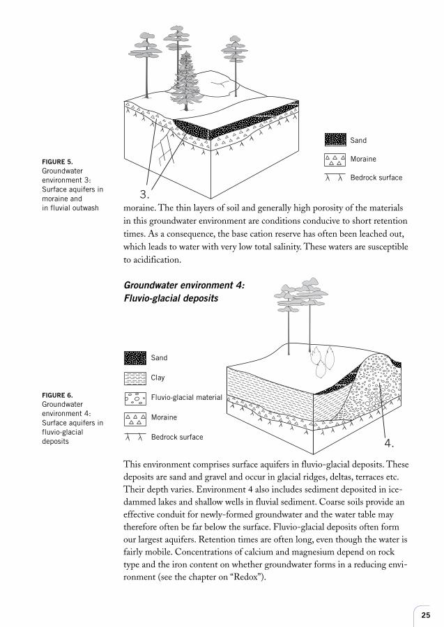
Groundwater environment 3: Moraine and fluvial outwashThis environment comprises surface aquifers in moraine and sediment. Thecomposition and thickness of the moraine varies. The water table is usuallyclose to the surface of the moraine owing to the low hydraulic conductivity ofthese materials. Fluvial outwash composition may also vary a great deal; theoutwash may be made up of gravel, sand or silt. The thickness varies, but isusually only 1 - 2 metres. Fluvial outwash occurs in deposits below the eleva-tion of the highest coastline in conjunction with fluvio-glacial deposits and

Sand

Clay

Fluvio-glacial material

Moraine

Limestone

Shale

Sandstone

25

moraine. The thin layers of soil and generally high porosity of the materialsin this groundwater environment are conditions conducive to short retentiontimes. As a consequence, the base cation reserve has often been leached out,which leads to water with very low total salinity. These waters are susceptibleto acidification.

Groundwater environment 4:Fluvio-glacial deposits

FIGURE 5.Groundwaterenvironment 3:Surface aquifers inmoraine andin fluvial outwash

Morän

Berggrundsyta

Sand

3.

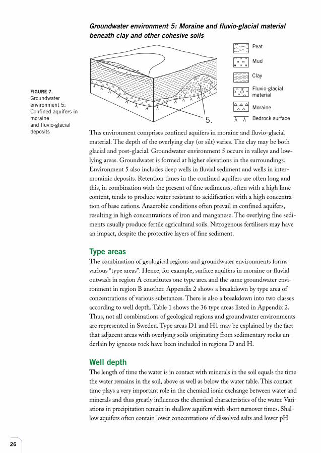
FIGURE 6.Groundwaterenvironment 4:Surface aquifers influvio-glacialdeposits

This environment comprises surface aquifers in fluvio-glacial deposits. Thesedeposits are sand and gravel and occur in glacial ridges, deltas, terraces etc.Their depth varies. Environment 4 also includes sediment deposited in ice-dammed lakes and shallow wells in fluvial sediment. Coarse soils provide aneffective conduit for newly-formed groundwater and the water table maytherefore often be far below the surface. Fluvio-glacial deposits often formour largest aquifers. Retention times are often long, even though the water isfairly mobile. Concentrations of calcium and magnesium depend on rocktype and the iron content on whether groundwater forms in a reducing envi-ronment (see the chapter on “Redox”).

Sand

Moraine

Bedrock surface

Sand

Clay

Fluvio-glacial material

Moraine

Bedrock surface4.

26

FIGURE 7.Groundwaterenvironment 5:Confined aquifers inmoraineand fluvio-glacialdeposits

Lera

Gyttja

Morän

Torv

Berggrundsyta

Isälvsmaterial

" " "" "" " " " " " " " "

" " " " " " "

"

" "

"

5.

This environment comprises confined aquifers in moraine and fluvio-glacialmaterial. The depth of the overlying clay (or silt) varies. The clay may be bothglacial and post-glacial. Groundwater environment 5 occurs in valleys and low-lying areas. Groundwater is formed at higher elevations in the surroundings.Environment 5 also includes deep wells in fluvial sediment and wells in inter-morainic deposits. Retention times in the confined aquifers are often long andthis, in combination with the present of fine sediments, often with a high limecontent, tends to produce water resistant to acidification with a high concentra-tion of base cations. Anaerobic conditions often prevail in confined aquifers,resulting in high concentrations of iron and manganese. The overlying fine sedi-ments usually produce fertile agricultural soils. Nitrogenous fertilisers may havean impact, despite the protective layers of fine sediment.

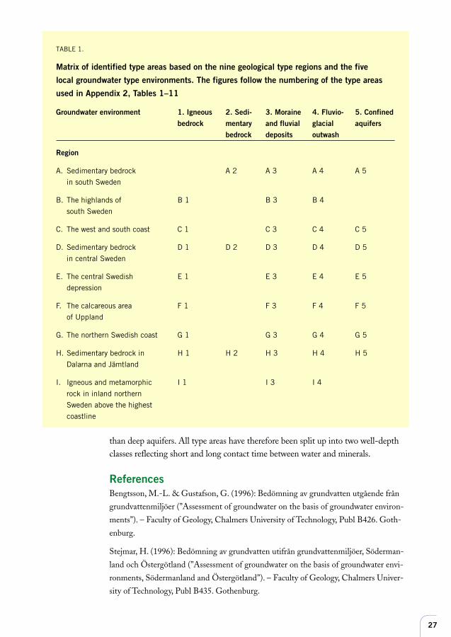
Type areasThe combination of geological regions and groundwater environments formsvarious “type areas”. Hence, for example, surface aquifers in moraine or fluvialoutwash in region A constitutes one type area and the same groundwater envi-ronment in region B another. Appendix 2 shows a breakdown by type area ofconcentrations of various substances. There is also a breakdown into two classesaccording to well depth. Table 1 shows the 36 type areas listed in Appendix 2.Thus, not all combinations of geological regions and groundwater environmentsare represented in Sweden. Type areas D1 and H1 may be explained by the factthat adjacent areas with overlying soils originating from sedimentary rocks un-derlain by igneous rock have been included in regions D and H.

Well depthThe length of time the water is in contact with minerals in the soil equals the timethe water remains in the soil, above as well as below the water table. This contacttime plays a very important role in the chemical ionic exchange between water andminerals and thus greatly influences the chemical characteristics of the water. Vari-ations in precipitation remain in shallow aquifers with short turnover times. Shal-low aquifers often contain lower concentrations of dissolved salts and lower pH

Groundwater environment 5: Moraine and fluvio-glacial materialbeneath clay and other cohesive soils

Peat

Mud

Clay

Fluvio-glacialmaterial

Moraine

Bedrock surface

27

than deep aquifers. All type areas have therefore been split up into two well-depthclasses reflecting short and long contact time between water and minerals.

ReferencesBengtsson, M.-L. & Gustafson, G. (1996): Bedömning av grundvatten utgående från

grundvattenmiljöer (”Assessment of groundwater on the basis of groundwater environ-

ments”). – Faculty of Geology, Chalmers University of Technology, Publ B426. Goth-

enburg.

Stejmar, H. (1996): Bedömning av grundvatten utifrån grundvattenmiljöer, Söderman-

land och Östergötland (”Assessment of groundwater on the basis of groundwater envi-

ronments, Södermanland and Östergötland”). – Faculty of Geology, Chalmers Univer-

sity of Technology, Publ B435. Gothenburg.

TABLE 1.

Matrix of identified type areas based on the nine geological type regions and the five

local groundwater type environments. The figures follow the numbering of the type areas

used in Appendix 2, Tables 1–11

Groundwater environment 1. Igneous 2. Sedi- 3. Moraine 4. Fluvio- 5. Confinedbedrock mentary and fluvial glacial aquifers

bedrock deposits outwash

Region

A. Sedimentary bedrock A 2 A 3 A 4 A 5

in south Sweden

B. The highlands of B 1 B 3 B 4

south Sweden

C. The west and south coast C 1 C 3 C 4 C 5

D. Sedimentary bedrock D 1 D 2 D 3 D 4 D 5

in central Sweden

E. The central Swedish E 1 E 3 E 4 E 5

depression

F. The calcareous area F 1 F 3 F 4 F 5

of Uppland

G. The northern Swedish coast G 1 G 3 G 4 G 5

H. Sedimentary bedrock in H 1 H 2 H 3 H 4 H 5

Dalarna and Jämtland

I. Igneous and metamorphic I 1 I 3 I 4

rock in inland northern

Sweden above the highest

coastline

28

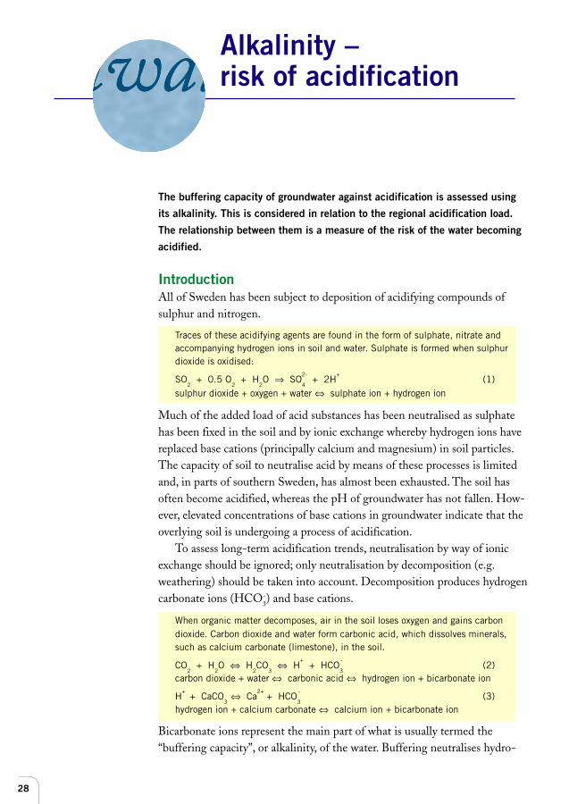
The buffering capacity of groundwater against acidification is assessed using

its alkalinity. This is considered in relation to the regional acidification load.

The relationship between them is a measure of the risk of the water becoming

acidified.

IntroductionAll of Sweden has been subject to deposition of acidifying compounds ofsulphur and nitrogen.

Traces of these acidifying agents are found in the form of sulphate, nitrate andaccompanying hydrogen ions in soil and water. Sulphate is formed when sulphurdioxide is oxidised:

SO2 + 0.5 O

2 + H

2O ⇒ SO

4

2- + 2H

+(1)

sulphur dioxide + oxygen + water ⇔ sulphate ion + hydrogen ion

Much of the added load of acid substances has been neutralised as sulphatehas been fixed in the soil and by ionic exchange whereby hydrogen ions havereplaced base cations (principally calcium and magnesium) in soil particles.The capacity of soil to neutralise acid by means of these processes is limitedand, in parts of southern Sweden, has almost been exhausted. The soil hasoften become acidified, whereas the pH of groundwater has not fallen. How-ever, elevated concentrations of base cations in groundwater indicate that theoverlying soil is undergoing a process of acidification.

To assess long-term acidification trends, neutralisation by way of ionicexchange should be ignored; only neutralisation by decomposition (e.g.weathering) should be taken into account. Decomposition produces hydrogencarbonate ions (HCO3

-) and base cations.

When organic matter decomposes, air in the soil loses oxygen and gains carbondioxide. Carbon dioxide and water form carbonic acid, which dissolves minerals,such as calcium carbonate (limestone), in the soil.

CO2 + H

2O ⇔ H

2CO

3 ⇔ H

+ + HCO

3

-(2)

carbon dioxide + water ⇔ carbonic acid ⇔ hydrogen ion + bicarbonate ion

H+ + CaCO

3 ⇔ Ca

2+ + HCO

3

-(3)

hydrogen ion + calcium carbonate ⇔ calcium ion + bicarbonate ion

Bicarbonate ions represent the main part of what is usually termed the“buffering capacity”, or alkalinity, of the water. Buffering neutralises hydro-

Alkalinity –risk of acidification

29

gen ions and reduces alkalinity, ie, reaction (2) goes in the other direction.Hence, resistance to acidification is largely determined by how easily the mi-nerals in the bedrock and in the soils in the catchment area of a well can bebroken down. In areas where soils and rocks are slow to break down (ie, with-out carbonate), the rate of weathering increases only marginally at lower pHlevels. Weathering capacity can be measured directly in well water as the levelof alkalinity.

However, the alkalinity buffering capacity of the water has been used up inareas where the soil no longer offers any protection against acidification. Al-kalinity declines in these wells to a level where pH also begins to fall. Acidifi-cation of groundwater means that more aluminium and heavy metals will bedissolved in the groundwater and also increases corrosion of piping, which inturn leads to higher metal concentrations in drinking water.

pH readings are highly unreliable, particularly if taken directly in the field.Alkalinity should instead be recorded as a means of assessing the bufferingcapacity of groundwater against acidification. Alkalinity principally comprisesHCO3

- and is a robust parameter that does not usually change between samp-ling and analysis. The pH of the groundwater can be estimated on the basis ofits alkalinity. Table 2 shows normal pH intervals in groundwater for the vari-ous alkalinity classes. (See Appendix 5 for more information on the choice ofparameters.)

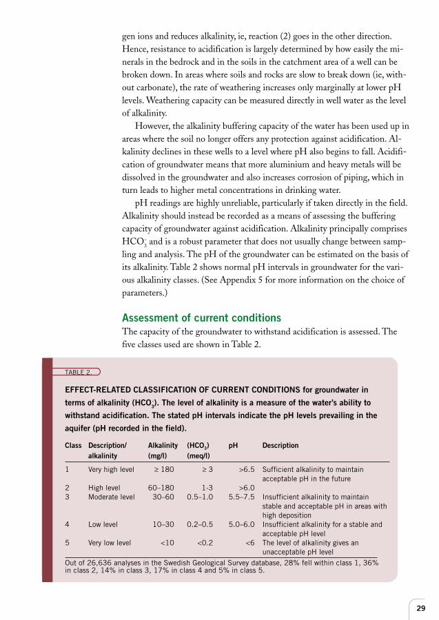
Assessment of current conditionsThe capacity of the groundwater to withstand acidification is assessed. Thefive classes used are shown in Table 2.

TABLE 2.

EFFECT-RELATED CLASSIFICATION OF CURRENT CONDITIONS for groundwater in

terms of alkalinity (HCO3-). The level of alkalinity is a measure of the water’s ability to

withstand acidification. The stated pH intervals indicate the pH levels prevailing in the

aquifer (pH recorded in the field).

Class Description/ Alkalinity (HCO3) pH Descriptionalkalinity (mg/l) (meq/l)

1 Very high level ≥ 180 ≥ 3 >6.5 Sufficient alkalinity to maintainacceptable pH in the future

2 High level 60–180 1-3 >6.03 Moderate level 30–60 0.5–1.0 5.5–7.5 Insufficient alkalinity to maintain

stable and acceptable pH in areas withhigh deposition

4 Low level 10–30 0.2–0.5 5.0–6.0 Insufficient alkalinity for a stable andacceptable pH level

5 Very low level <10 <0.2 <6 The level of alkalinity gives anunacceptable pH level

Out of 26,636 analyses in the Swedish Geological Survey database, 28% fell within class 1, 36%in class 2, 14% in class 3, 17% in class 4 and 5% in class 5.

30

Guide and limit values for drinking water issued by the NationalFood Administration (see also Appendix 11)Guide value: 60 mg/l (1 meq/l) HCO3

-

Limit value (technical reservations, acceptable): 30 mg/l (0.5 meq/l) HCO3-

The boundaries between classes 2–3 and 3–4 are effect-related. Other classboundaries have been selected to provide a good degree of accuracy onboth sides of the guide and limit values.

If extensive corrosion of piping and resulting elevated metal concentrationsare to be avoided (see also the chapter on “Metals”), the pH of the watershould be higher than 6.0, which means that alkalinity should be greaterthan 30 mg/l (0.5 meq/l). Many Swedish wells fail to meet these stan-dards. In some of these the groundwater is naturally acid. The naturalcarbonic acid in the water causes low pH in shallow wells in areas with lowweathering capacity. Wells bored in rock usually have higher alkalinity(HCO3

-) than wells bored through loose deposits.

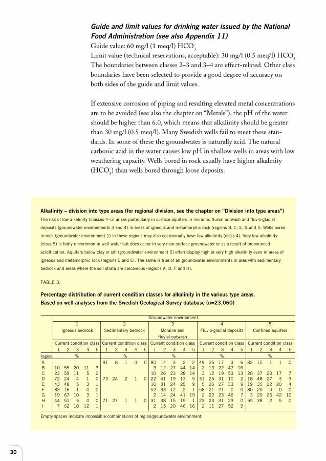
TABLE 3.

Percentage distribution of current condition classes for alkalinity in the various type areas.Based on well analyses from the Swedish Geological Survey database (n=23,060)

Groundwater environment1 2 3 4 5

Igneous bedrock Sedimentary bedrock Moraine and Fluvio-glacial deposits Confined aquifersfluvial outwash

Current condition class Current condition class Current condition class Current condition class Current condition class1 2 3 4 5 1 2 3 4 5 1 2 3 4 5 1 2 3 4 5 1 2 3 4 5

Region % % % % % A 91 8 1 0 0 80 14 3 2 2 49 26 17 3 6 83 15 1 1 0 B 10 55 20 11 3 3 12 27 44 14 2 13 22 47 16 C 23 59 11 5 2 10 26 23 28 14 3 12 19 53 13 20 37 20 17 7 D 72 24 4 1 0 73 24 2 1 0 22 41 19 13 5 31 25 31 10 2 18 48 27 3 3 E 43 48 5 3 1 10 31 24 25 9 5 26 27 33 9 19 35 22 20 4 F 83 16 1 0 0 52 33 12 2 1 58 21 21 0 0 80 20 0 0 0 G 19 67 10 3 1 2 14 24 41 19 2 22 23 46 7 3 20 26 42 10 H 44 51 5 0 0 71 27 1 1 0 31 38 15 15 1 23 23 31 23 0 55 38 2 5 0 I 7 62 18 12 1 2 15 20 46 16 2 11 27 52 9

Empty spaces indicate impossible combinations of region/groundwater environment.

Alkalinity – division into type areas (for regional division, see the chapter on “Division into type areas”)The risk of low alkalinity (classes 4–5) arises particularly in surface aquifers in moraine, fluvial outwash and fluvio-glacial

deposits (groundwater environments 3 and 4) in areas of igneous and metamorphic rock (regions B, C, E, G and I). Wells bored

in rock (groundwater environment 1) in these regions may also occasionally have low alkalinity (class 4). Very low alkalinity

(class 5) is fairly uncommon in well water but does occur in very near-surface groundwater or as a result of pronounced

acidification. Aquifers below clay or silt (groundwater environment 5) often display high or very high alkalinity even in areas of

igneous and metamorphic rock (regions C and E). The same is true of all groundwater environments in ares with sedimentary

bedrock and areas where the soil strata are calcareous (regions A, D, F and H).

31

Reference valueIt is very difficult to calculate original and exhausted alkalinity in a givenbody of groundwater owing to great local differences in sulphate load,mineralogy and flow patterns. Average regional figures for sulphate depo-sition valid for a given point in time can be derived, but when it comes toassessing a given well (or a limited number of wells), difficulties will arise,since their response to the acidification load will vary. There is therefore noreference value for “Alkalinity – risk of acidification”.

Assessment of risk of acidificationThe capacity of groundwater to withstand acidification is assessed in rela-tion to the acidification load. In the past, the ratio between alkalinity andtotal hardness was frequently used to determine the degree of acidificationimpact. This model has now been abandoned. Instead, the residual capaci-ty of the water to withstand acifidication (ie, its alkalinity) is comparedwith the acidification load in the form of sulphur deposition (for the rea-sons for this, see Appendix 5).

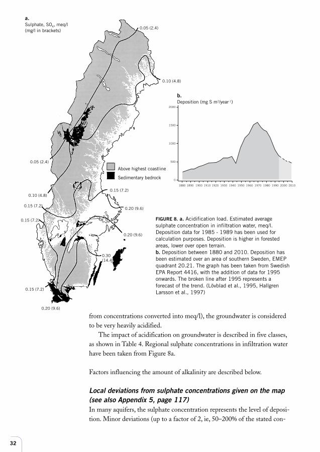
Regional airborne sulphur deposition (not including sea salts) is used asa measure of the acidification load. Since airborne nitrogen deposition todate has been largely absorbed by vegetation, the direct acidifying effect ofnitrogen has been limited. The acidification load has therefore been de-rived solely from regional sulphate deposition figures. Deposition data for1985 - 1989 has been used for the load map (Figure 8a). Sulphur deposi-tion has been converted into a numerical value for the sulphate concentra-tion in the precipitation infiltrating into the groundwater, using meanfigures for the annual flow. For calculation purposes, annual flow is as-sumed to correspond to annual groundwater formation. The acidificationload on a given well may be lower or higher, depending on local depositionand water turnover conditions. Deposition has been calculated for theaverage land use in the area. In areas exclusively covered by forest, deposi-tion will be greater owing to high dry deposition. In south-west Sweden,which has high precipitation levels and hence a high rate of groundwateraccumulation, concentrations are lower than in the south-east of the coun-try. Wells have been affected by acid deposition to varying degrees. Apartfrom the amount of deposition, the degree of impact also depends on thebuffering capacity of the well water, which is in turn dependent on thedegree of weathering taking place in its catchment area. Sulphur deposi-tion peaked in the 1970s, but although it has decreased, it remains farhigher than natural background levels (Figure 8b).

The alkalinity of the groundwater sample is compared with the acidifi-cation load to assess the acidification impact. If the acidification load fromdeposition is as great or greater than the buffering capacity (calculated

32

from concentrations converted into meq/l), the groundwater is consideredto be very heavily acidified.

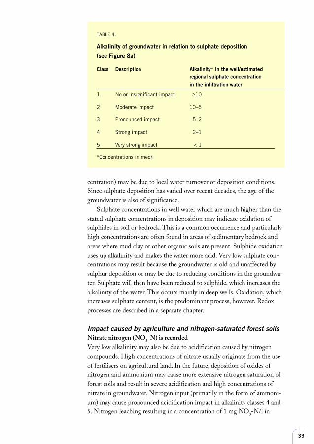
The impact of acidification on groundwater is described in five classes,as shown in Table 4. Regional sulphate concentrations in infiltration waterhave been taken from Figure 8a.

Factors influencing the amount of alkalinity are described below.

Local deviations from sulphate concentrations given on the map(see also Appendix 5, page 117)In many aquifers, the sulphate concentration represents the level of deposi-tion. Minor deviations (up to a factor of 2, ie, 50–200% of the stated con-

FIGURE 8. a. Acidification load. Estimated averagesulphate concentration in infiltration water, meq/l.Deposition data for 1985 - 1989 has been used forcalculation purposes. Deposition is higher in forestedareas, lower over open terrain.b. Deposition between 1880 and 2010. Deposition hasbeen estimated over an area of southern Sweden, EMEPquadrant 20.21. The graph has been taken from SwedishEPA Report 4416, with the addition of data for 1995onwards. The broken line after 1995 represents aforecast of the trend. (Lövblad et al., 1995, HallgrenLarsson et al., 1997)

Deposition (mg S m2 år-1)2000

1500

1000

500

0

1880 1890 1900 1910 1920 1930 1940 1950 1960 1970 1980 1990 2000 2010

a.Sulphate, SO4, meq/l(mg/l in brackets)

b.Deposition (mg S m2/year-1)

Above highest coastline

Sedimentary bedrock

0.10 (4.8)

0.10 (4.8)

0.05 (2.4)

0.05 (2.4)

0.15 (7.2)

0.15 (7.2)

0.15 (7.2)

0.20 (9.6)

0.20 (9.6)

0.30(14.4)

0.15 (7.2)

0.20 (9.6)

33

centration) may be due to local water turnover or deposition conditions.Since sulphate deposition has varied over recent decades, the age of thegroundwater is also of significance.

Sulphate concentrations in well water which are much higher than thestated sulphate concentrations in deposition may indicate oxidation ofsulphides in soil or bedrock. This is a common occurrence and particularlyhigh concentrations are often found in areas of sedimentary bedrock andareas where mud clay or other organic soils are present. Sulphide oxidationuses up alkalinity and makes the water more acid. Very low sulphate con-centrations may result because the groundwater is old and unaffected bysulphur deposition or may be due to reducing conditions in the groundwa-ter. Sulphate will then have been reduced to sulphide, which increases thealkalinity of the water. This occurs mainly in deep wells. Oxidation, whichincreases sulphate content, is the predominant process, however. Redoxprocesses are described in a separate chapter.

Impact caused by agriculture and nitrogen-saturated forest soilsNitrate nitrogen (NO3-N) is recordedVery low alkalinity may also be due to acidification caused by nitrogencompounds. High concentrations of nitrate usually originate from the useof fertilisers on agricultural land. In the future, deposition of oxides ofnitrogen and ammonium may cause more extensive nitrogen saturation offorest soils and result in severe acidification and high concentrations ofnitrate in groundwater. Nitrogen input (primarily in the form of ammoni-um) may cause pronounced acidification impact in alkalinity classes 4 and5. Nitrogen leaching resulting in a concentration of 1 mg NO3-N/l in

TABLE 4.

Alkalinity of groundwater in relation to sulphate deposition

(see Figure 8a)

Class Description Alkalinity* in the well/estimatedregional sulphate concentrationin the infiltration water

1 No or insignificant impact ≥10

2 Moderate impact 10–5

3 Pronounced impact 5–2

4 Strong impact 2–1

5 Very strong impact < 1

*Concentrations in meq/l

34

groundwater may cause an acidification effect of up to 0.07–0.14 meq/l.This will add to the regional acidification load deriving from sulphur (asshown on the map in Figure 8a).

ReferencesAastrup, M., Berntell, A., Bertills, U., Johnson, J. & Thunholm, B. (1995):

Groundwater chemistry in Sweden. – Swedish Environmental Protection Agency

Report 4416.

Lövblad, G. et al. (1992): Mapping deposition of sulphur, nitrogen and base ca-

tions in the nordic countries. – Swedish Environmental Research Institute, Report

B 1055.

Lövblad, G. (1990): Luftföroreningshalter och deposition i bakgrundsluft (”Con-

centrations of air pollutants and deposition in background air”). – Swedish Envi-

ronmental Protection Agency Report 3812, 1990:14.

Bertills, U., Hanneberg, P. (1995): Acidification in Sweden – What do we really

know? – Swedish Environmental Protection Agency Report 4422.

Trends in sulphur depositionHallgren Larsson, E., Knulst, J.C., Lövblad, G., Malm, G., Sjöberg, K. & West-

ling, O. (1997): Luftföroreningar i södra Sverige 1985–1995 (”Air pollution in

southern Sweden 1985–1995”). – Swedish Environmental Research Institute,

Report B 1257.

Lövblad, G., Kindborn, K., Grennfelt, P., Hultberg, H. & Westling, O. (1995):

Deposition of acidifying substances in Sweden. From: Staaf, H. & Tyler, G. (Eds.)

Effects of acid deposition and tropospheric ozone on forest ecosystems in Sweden.

– Ecological Bulletins 44:17–34.

Deposition dataSwedish Environmental Research Institute (IVL)

Land use dataNational Forest Survey

Flow dataSwedish Meteorological and Hydrological Institute (SMHI)

35

The nitrogen content of groundwater is assessed in terms of the concentra-

tion of nitrate.

IntroductionHigh concentrations of nitrogen compounds limit the utility of ground-water for drinking purposes owing to health risks. Natural concentrationsof nitrogen compounds in groundwater are very low, since nitrogen is nor-mally in short supply, being absorbed by vegetation. Elevated concentra-tions usually result from the use of farmyard manure, nitrogenous ferti-lisers (particularly on agricultural land) or the impact of sewage. Deposi-tion of airborne nitrogen is high in southern Sweden. Nitrogen depositionoriginates from emissions of nitrogen oxides (mainly from traffic, wherethey are a by-product of combustion) and ammonia (almost all of whichoriginates from livestock farming). Most airborne nitrogen has so far beenabsorbed by vegetation.

Nitrogen occurs mainly as nitrate in groundwater. The nitrate ion isscarcely adsorbed to soil particles and is therefore highly mobile in soil andgroundwater. Elevated nitrate concentrations commonly occur in shallowwells. High levels of nitrogen may be lowered by various reduction proces-ses, particularly in deep wells with anaerobic conditions (see the chapter on“Redox” and Appendix 6). Nitrate reduction by denitrification may occurwhere groundwater flows into wetlands, liberating gaseous nitrogen intothe atmosphere in the process. However, elevated concentrations of nitro-gen in groundwater generally mean that the amount of this element enter-ing surface watercourses and the sea will increase.

The state of groundwater in terms of nitrogen compounds is presentedhere as the concentration of nitrate nitrogen (NO3-N). Elevated concen-trations of nitrite nitrogen (NO2-N) and ammonium nitrogen (NH4-N)may occur under reducing conditions (class 4 in Table 11 in the “Redox”chapter and Appendix 6) but concentrations are generally lower than thoseof nitrate. Organic nitrogen in groundwater is not usually determined.

Nitrogen

36

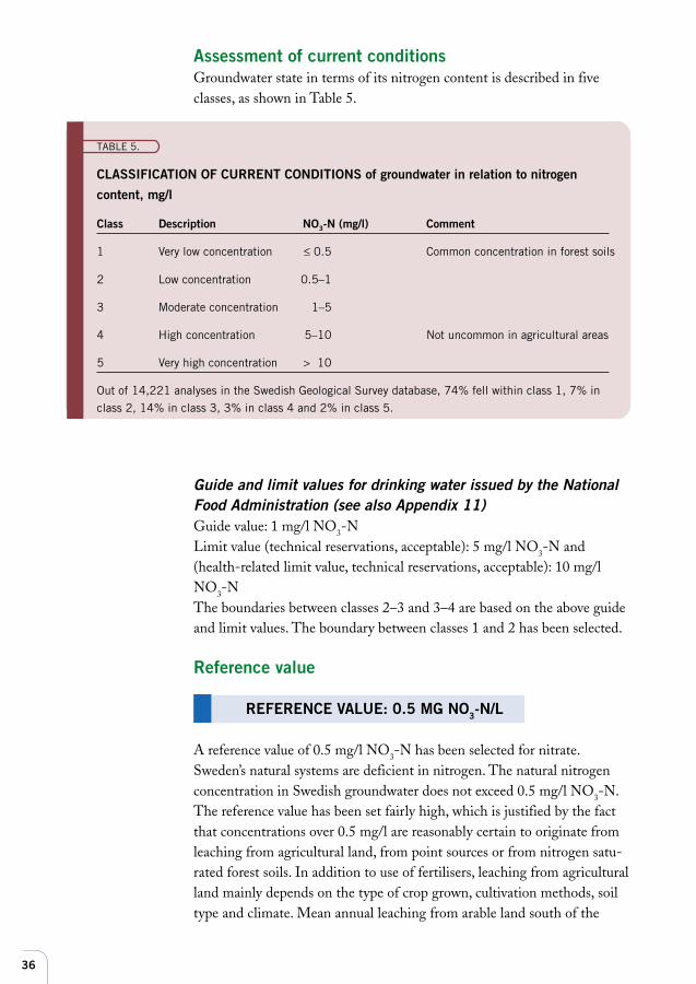
TABLE 5.

CLASSIFICATION OF CURRENT CONDITIONS of groundwater in relation to nitrogen

content, mg/l

Class Description NO3-N (mg/l) Comment

1 Very low concentration ≤ 0.5 Common concentration in forest soils

2 Low concentration 0.5–1

3 Moderate concentration 1–5

4 High concentration 5–10 Not uncommon in agricultural areas

5 Very high concentration > 10

Out of 14,221 analyses in the Swedish Geological Survey database, 74% fell within class 1, 7% in

class 2, 14% in class 3, 3% in class 4 and 2% in class 5.

Guide and limit values for drinking water issued by the NationalFood Administration (see also Appendix 11)Guide value: 1 mg/l NO3-NLimit value (technical reservations, acceptable): 5 mg/l NO3-N and(health-related limit value, technical reservations, acceptable): 10 mg/lNO3-NThe boundaries between classes 2–3 and 3–4 are based on the above guideand limit values. The boundary between classes 1 and 2 has been selected.

Reference value

REFERENCE VALUE: 0.5 MG NO3-N/L

A reference value of 0.5 mg/l NO3-N has been selected for nitrate.Sweden’s natural systems are deficient in nitrogen. The natural nitrogenconcentration in Swedish groundwater does not exceed 0.5 mg/l NO3-N.The reference value has been set fairly high, which is justified by the factthat concentrations over 0.5 mg/l are reasonably certain to originate fromleaching from agricultural land, from point sources or from nitrogen satu-rated forest soils. In addition to use of fertilisers, leaching from agriculturalland mainly depends on the type of crop grown, cultivation methods, soiltype and climate. Mean annual leaching from arable land south of the

Assessment of current conditionsGroundwater state in terms of its nitrogen content is described in fiveclasses, as shown in Table 5.

37

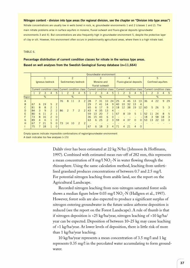
Nitrogen content - division into type areas (for regional division, see the chapter on “Division into type areas”)Nitrate concentrations are usually low in wells bored in rock, ie, groundwater environments 1 and 2 (classes 1 and 2). The

main nitrate problems arise in surface aquifers in moraine, fluvial outwash and fluvio-glacial deposits (groundwater

environments 3 and 4). But concentrations are also frequently high in groundwater environment 5, despite the protective layer

of clay or silt. However, this environment often occurs in predominantly agricultural areas, where there is a high nitrate load.

TABLE 6.

Percentage distribution of current condition classes for nitrate in the various type areas.

Based on well analyses from the Swedish Geological Survey database (n=11,664)




Region % % % % %

A 76 8 11 3 2 28 7 31 10 24 25 4 46 13 13 36 4 22 9 29 B 67 6 19 5 2 29 7 41 14 9 40 10 32 13 4 C 81 8 8 2 1 65 6 17 9 3 18 12 38 19 12 60 5 26 5 3 D 84 3 9 2 2 86 2 7 2 2 43 4 35 13 4 - - - - - - - - - - E 80 6 11 2 1 59 13 20 7 1 67 8 19 5 1 52 11 24 8 5 F 73 8 16 2 0 36 15 43 6 0 - - - - - 18 3 58 18 3 G 89 4 6 1 0 63 6 25 2 3 59 4 37 0 0 53 13 22 10 3 H 67 7 21 5 0 73 14 10 2 2 - - - - - - - - - - - - - - - I 75 7 18 1 0 67 6 18 3 4 71 4 21 4 0

Empty spaces indicate impossible combinations of region/groundwater environmentA dash indicates too few analyses (<15)

Dalälv river has been estimated at 22 kg N/ha ( Johnsson & Hoffmann,1997). Combined with estimated mean run-off of 282 mm, this representsa mean concentration of 8 mg/l NO3-N in water flowing through therhizosphere. Using the same calculation method, leaching from unferti-lised grassland produces concentrations of between 0.7 and 2.5 mg/l.For potential nitrogen leaching from arable land, see the report on theAgricultural Landscape.

Recorded nitrogen leaching from non-nitrogen saturated forest soilsshows a median figure below 0.03 mg/l NO3-N (Hallgren et al., 1997).However, forest soils are also expected to produce a significant surplus ofnitrogen entering groundwater in the future unless airborne deposition isreduced (see the report on the Forest Landscape). A rule of thumb is thatif nitrogen deposition is >25 kg/ha/year, nitrogen leaching of >10 kg/ha/year can be expected. Deposition of between 10–25 kg may cause leachingof >1 kg/ha/year. At lower levels of deposition, there is little risk of morethan 1 kg/ha/year leaching.

10 kg/ha/year represents a mean concentration of 3.5 mg/l and 1 kgrepresents 0.35 mg/l in the percolated water accumulating to form ground-water.

38

Factors that may result in elevated nitrogen concentrations are describedbelow.

Impact from agriculture, sewage and landfill sitesPhosphate (PO4), potassium (K) and chloride (Cl) are recordedHigh concentrations of nitrate are sometime accompanied by elevatedconcentrations of the nutrients phosphate and potassium. Since both ofthese are tightly fixed in soil, elevated concentrations of phosphate(>0.1 mg/l) or potassium (>10 mg/l) in agricultural areas may indicaterapid passage between the soil surface and the groundwater. Althoughconcentrations above those indicated often derive from some kind ofanthropogenic impact, higher concentrations may also have natural causes.For example, high phosphate concentrations may occur naturally in anae-robic environments (see Appendix 6). Phosphate and potassium may origi-nate from fertilisers, sewage and landfill. Elevated chloride concentrations(see the chapter on “Salt – chloride”) may also accompany high nitrateconcentrations. This is common where sewage has an impact and at land-fill sites for household refuse.

Knowledge of land use, location of sewage treatment plants, manure/fertiliser stores, landfill sites etc is necessary to identify the probablesource(s) of elevated nitrogen concentrations in groundwater.

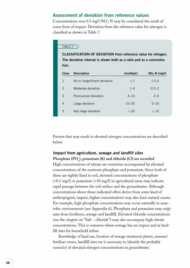
TABLE 7.

CLASSIFICATION OF DEVIATION from reference value for nitrogen.

The deviation interval is shown both as a ratio and as a concentra-

tion.

Class Description (multiple) NO3-N (mg/l)

1 No or insignificant deviation ≤ 1 ≤ 0.5

2 Moderate deviation 1–4 0.5–2

3 Pronounced deviation 4–10 2–5

4 Large deviation 10–20 5–10

5 Very large deviation > 20 > 10

Assessment of deviation from reference valuesConcentrations over 0.5 mg/l NO3-N may be considered the result ofsome form of impact. Deviation from the reference value for nitrogen isclassified as shown in Table 7.

39

ReferencesNitrogen in arable soilsJohnsson, H. & Hoffmann, M. (1997): Kväveläckage från svensk åkermark - be-

räkning av normalutlakning och möjliga åtgärdar. – Swedish EPA Report 4741.

Nitrogen in forest soilsHallgren Larsson, E., Knulst, J.C., Lövblad, G., Malm, G., Sjöberg, K. & West-

ling, O. (1997): Luftföroreningar i södra Sverige 1985–1995 (”Air pollution in

southern Sweden 1985–1995”). – Swedish Environmental Research Institute,

Report B 1257.

Lövblad, G. et al. (1992): Mapping deposition of sulphur, nitrogen and base ca-


B 1055.


centrations of air pollutants and deposition in background air”). – Swedish EPA

Report 3812, 1990:14.

40

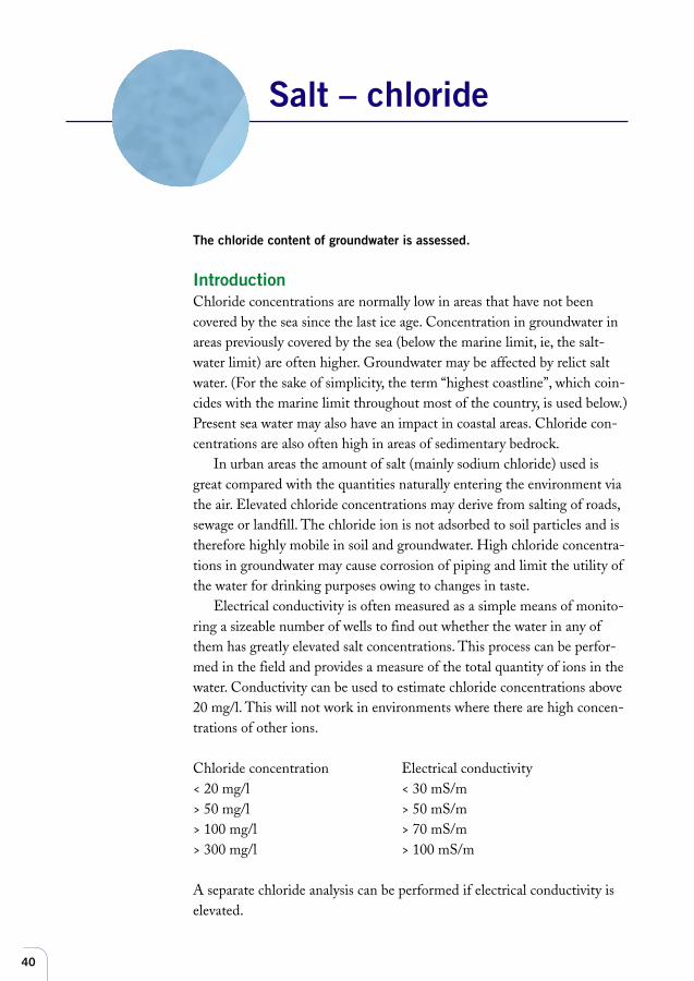
The chloride content of groundwater is assessed.

IntroductionChloride concentrations are normally low in areas that have not beencovered by the sea since the last ice age. Concentration in groundwater inareas previously covered by the sea (below the marine limit, ie, the salt-water limit) are often higher. Groundwater may be affected by relict saltwater. (For the sake of simplicity, the term “highest coastline”, which coin-cides with the marine limit throughout most of the country, is used below.)Present sea water may also have an impact in coastal areas. Chloride con-centrations are also often high in areas of sedimentary bedrock.

In urban areas the amount of salt (mainly sodium chloride) used isgreat compared with the quantities naturally entering the environment viathe air. Elevated chloride concentrations may derive from salting of roads,sewage or landfill. The chloride ion is not adsorbed to soil particles and istherefore highly mobile in soil and groundwater. High chloride concentra-tions in groundwater may cause corrosion of piping and limit the utility ofthe water for drinking purposes owing to changes in taste.

Electrical conductivity is often measured as a simple means of monito-ring a sizeable number of wells to find out whether the water in any ofthem has greatly elevated salt concentrations. This process can be perfor-med in the field and provides a measure of the total quantity of ions in thewater. Conductivity can be used to estimate chloride concentrations above20 mg/l. This will not work in environments where there are high concen-trations of other ions.

Chloride concentration Electrical conductivity< 20 mg/l < 30 mS/m> 50 mg/l > 50 mS/m> 100 mg/l > 70 mS/m> 300 mg/l > 100 mS/m

A separate chloride analysis can be performed if electrical conductivity iselevated.

Salt – chloride

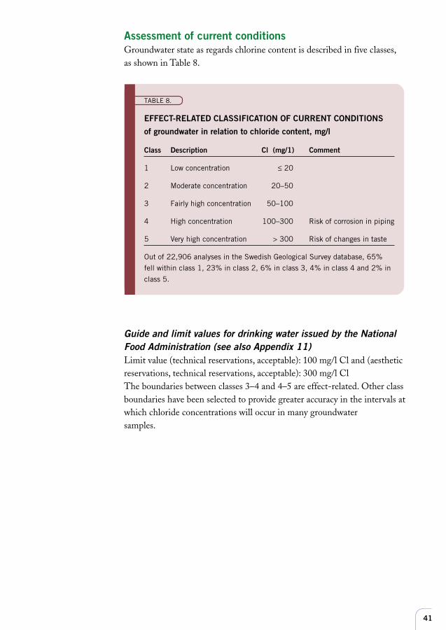
41

Guide and limit values for drinking water issued by the NationalFood Administration (see also Appendix 11)Limit value (technical reservations, acceptable): 100 mg/l Cl and (aestheticreservations, technical reservations, acceptable): 300 mg/l ClThe boundaries between classes 3–4 and 4–5 are effect-related. Other classboundaries have been selected to provide greater accuracy in the intervals atwhich chloride concentrations will occur in many groundwatersamples.

TABLE 8.

EFFECT-RELATED CLASSIFICATION OF CURRENT CONDITIONS

of groundwater in relation to chloride content, mg/l

Class Description Cl (mg/1) Comment

1 Low concentration ≤ 20

2 Moderate concentration 20–50

3 Fairly high concentration 50–100

4 High concentration 100–300 Risk of corrosion in piping

5 Very high concentration > 300 Risk of changes in taste

Out of 22,906 analyses in the Swedish Geological Survey database, 65%

fell within class 1, 23% in class 2, 6% in class 3, 4% in class 4 and 2% in

class 5.

Assessment of current conditionsGroundwater state as regards chlorine content is described in five classes,as shown in Table 8.

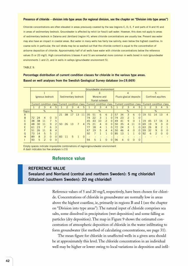
42

Presence of chloride – division into type areas (for regional division, see the chapter on “Division into type areas”)

Chloride concentrations are often elevated in areas previously covered by the sea (regions C, D, E, F and parts of A and H) and

in areas of sedimentary bedrock. Groundwater is affected by relict (or fossil) salt water. However, this does not apply to areas

of sedimentary bedrock in Dalarna and Jämtland (region H), where chloride concentrations are usually low. Present sea water

may also have an impact in coastal areas. But water in many wells has fairly low salinity, even below the highest coastline. In

coarse soils in particular, the soil strata may be so washed out that the chloride content is equal to the concentration of

airborne deposition of chloride. Approximately half of all wells have water with chloride concentrations below the reference

values (5 or 20 mg/l). High concentrations (classes 4 and 5) are somewhat more common in wells bored in rock (groundwater

environments 1 and 2), and in wells in valleys (groundwater environment 5).

TABLE 9.

Percentage distribution of current condition classes for chloride in the various type areas.

Based on well analyses from the Swedish Geological Survey database (n=19,669)




Region % % % % % A 21 38 17 13 11 35 51 6 6 2 57 34 3 6 0 19 51 14 13 4 B 72 24 4 0 0 74 22 3 1 0 74 23 2 1 0 C 38 38 11 7 5 45 43 10 2 0 49 41 9 0 1 19 45 17 16 3 D 48 30 11 9 2 50 26 13 7 4 75 21 4 0 0 50 35 4 11 0 69 19 9 3 0 E 61 23 7 6 3 77 18 4 1 0 72 24 3 1 0 63 26 8 2 1 F 51 26 11 8 4 67 19 5 4 4 50 46 4 0 0 59 32 9 0 0 G 73 14 5 5 2 92 7 1 1 0 85 13 1 1 0 92 6 2 0 0 H 89 8 3 0 0 83 11 5 1 0 - - - - - - - - - - - - - - - I 93 5 2 0 0 94 5 1 0 0 96 4 0 0 0


Reference value

Reference values of 5 and 20 mg/l, respectively, have been chosen for chlori-de. Concentrations of chloride in groundwater are normally low in areasabove the highest coastline, ie, primarily in regions B and I (see the chapteron “Division into type areas”). The natural input of chloride comprises seasalts, some dissolved in precipitation (wet deposition) and some falling asparticles (dry deposition). The map in Figure 9 shows the estimated con-centration of atmospheric deposition of chloride in the water infiltrating toform groundwater (for method of calculating concentrations, see page 31).

The mean figure for chloride in unaffected wells in a given area shouldbe at approximately this level. The chloride concentration in an individualwell may be higher or lower owing to local variations in deposition and infil-

REFERENCE VALUESvealand and Norrland (central and northern Sweden): 5 mg chloride/lGötaland (southern Sweden): 20 mg chloride/l

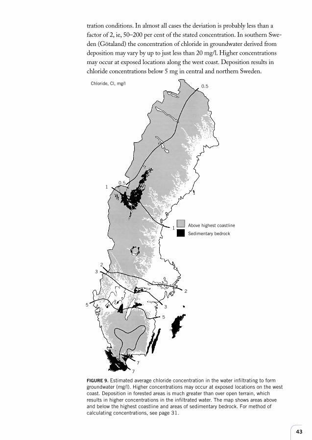
43

tration conditions. In almost all cases the deviation is probably less than afactor of 2, ie, 50–200 per cent of the stated concentration. In southern Swe-den (Götaland) the concentration of chloride in groundwater derived fromdeposition may vary by up to just less than 20 mg/l. Higher concentrationsmay occur at exposed locations along the west coast. Deposition results inchloride concentrations below 5 mg in central and northern Sweden.

FIGURE 9. Estimated average chloride concentration in the water infiltrating to formgroundwater (mg/l). Higher concentrations may occur at exposed locations on the westcoast. Deposition in forested areas is much greater than over open terrain, whichresults in higher concentrations in the infiltrated water. The map shows areas aboveand below the highest coastline and areas of sedimentary bedrock. For method ofcalculating concentrations, see page 31.

Chloride, Cl, mg/l

Above highest coastline

Sedimentary bedrock1

1

0.5

10.5

3

2

5

7

7

5

3

2

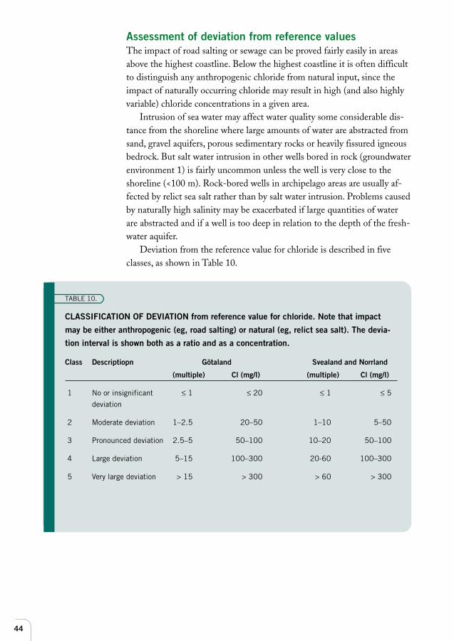
44

Assessment of deviation from reference valuesThe impact of road salting or sewage can be proved fairly easily in areasabove the highest coastline. Below the highest coastline it is often difficultto distinguish any anthropogenic chloride from natural input, since theimpact of naturally occurring chloride may result in high (and also highlyvariable) chloride concentrations in a given area.

Intrusion of sea water may affect water quality some considerable dis-tance from the shoreline where large amounts of water are abstracted fromsand, gravel aquifers, porous sedimentary rocks or heavily fissured igneousbedrock. But salt water intrusion in other wells bored in rock (groundwaterenvironment 1) is fairly uncommon unless the well is very close to theshoreline (<100 m). Rock-bored wells in archipelago areas are usually af-fected by relict sea salt rather than by salt water intrusion. Problems causedby naturally high salinity may be exacerbated if large quantities of waterare abstracted and if a well is too deep in relation to the depth of the fresh-water aquifer.

Deviation from the reference value for chloride is described in fiveclasses, as shown in Table 10.

TABLE 10.

CLASSIFICATION OF DEVIATION from reference value for chloride. Note that impact

may be either anthropogenic (eg, road salting) or natural (eg, relict sea salt). The devia-

tion interval is shown both as a ratio and as a concentration.

Class Descriptiopn Götaland Svealand and Norrland

(multiple) Cl (mg/l) (multiple) Cl (mg/l)

1 No or insignificant ≤ 1 ≤ 20 ≤ 1 ≤ 5

deviation

2 Moderate deviation 1–2.5 20–50 1–10 5–50

3 Pronounced deviation 2.5–5 50–100 10–20 50–100

4 Large deviation 5–15 100–300 20-60 100–300

5 Very large deviation > 15 > 300 > 60 > 300

45

Factors that may result in elevated chloride concentrations are describedbelow. These may help to trace the cause.

Impact of salt waterThe relationship between chloride, sodium, calcium and magnesium isexamined. Any elevated sulphate concentrations are examined.Not only does water in wells affected by salt water have a high chlorideconcentration, it may display other chemical differences as compared withwater in wells not affected by salt water. These include differences in theproportions of ions of chloride, sodium, calcium, magnesium and sulphate.The sulphate content is usually higher than the deposition level in ground-water affected by salt water (see Figure 8a).

The chloride content of sea water is matched by a sodium contentrepresenting 85 per cent of the chloride content (in equivalents). Largeflows and rapid passage between sea water and a well may cause the salinegroundwater to display the same ratio of sodium to chloride as in sea wa-ter. This is probably unusual, however. Ion exchange usually occurs wheresodium ions are replaced by those of calcium and magnesium.

Water in a well affected by relict salt water instead sometimes has asodium content higher than its chloride content (in equivalents) and highalkalinity (>180 mg/l HCO3).

Elevated salinity may occur in environments where salts are leachedout from clays overlying the aquifer. The groundwater may have elevatedconcentrations of calcium and magnesium as a result of ion exchange.

Sedimentary bedrockSulphur content is recordedSedimentary bedrock, interspersed with shale, for example, exhibits natu-rally elevated sulphate concentrations (see the chapter on “Division intotype areas”, Figure 2, showing geological regions).

Salting of roads in winterThe relationship between chloride, sodium and total hardness is examinedWhere road salting has had an impact, a sodium chloride ratio of 1:1 (cal-culated as equivalents) may be expected. However, the situation may becomplicated by ion exchange in the soil, so that calcium and magnesiumconcentrations (total hardness) increase instead of sodium.

Sewage, landfill sites and livestock farmingNitrogen content is recordedElevated chloride concentrations due to impact from sewage, landfill orlivestock farming are often accompanied by elevated concentrations ofnitrate and ammonium (see the chapter on “Nitrogen”).

46

ReferencesLövblad, G. et al. (1992): Mapping deposition of sulphur, nitrogen and base ca-


B 1055.


centrations of air pollutants and deposition in background air”). – Swedish Envi-

ronmental Protection Agency Report 3812, 1990:14.

Olofsson, B. (1996): Salt groundwater in Sweden – occurrence and origin.

SWIM-96, Salt Water Intrusion Meeting. – Swedish Geological Survey Reports

and Notices, No. 87, pp 91–100.

Deposition dataSwedish Environmental Research Institute (IVL)

Land use dataNational Forest Survey

Flow dataSwedish Meteorological and Hydrological Institute (SMHI)

47

Redox conditions in groundwater have a great influence on the solubility of

many substances and hence concentrations in the water. Redox is assessed

on the basis of the relative concentrations of ion, manganese and sulphate

in the water.

IntroductionThe term REDOX represents a large number of chemical reactions invol-ving electron transfer. When a substance is OXidised, it transfers electronsto another substance, which is then REDuced. Many redox reactions areextremely slow unless catalysed by bacteria. The point at which a givenreaction can take place is determined by the electrical tension difference orredox potential in the water - Eh. Eh may be seen as a measure of thepropulsive force for the reaction. Redox potential can be measured directlyin the water, although this is difficult. Instead, it has been decided to esti-mate the redox potential of the water by studying the relative concentra-tions of iron, manganese and sulphate. They appear in aqueous solutionwithin specific redox intervals and, taken together, give a narrower range inwhich the solubility conditions for all three are met. These parametershave been chosen because they normally occur in fairly high concentra-tions in most natural groundwater systems. These substances thereforeprovide a robust system of assessment.

The redox status of the water provides information about problems tobe expected when water is pumped up from the well. It may show whetherthe water will be difficult to treat to remove dissolved iron and manganese,whether the water will emit hydrogen sulphide or methane and whetheriron and manganese will be precipitated. See Appendix 6 for a more detai-led description of redox potential - Eh and redox reactions in the environ-ment.

Assessment of current conditionsGroundwater redox status is described in five classes, as shown in Table 11.

Redox

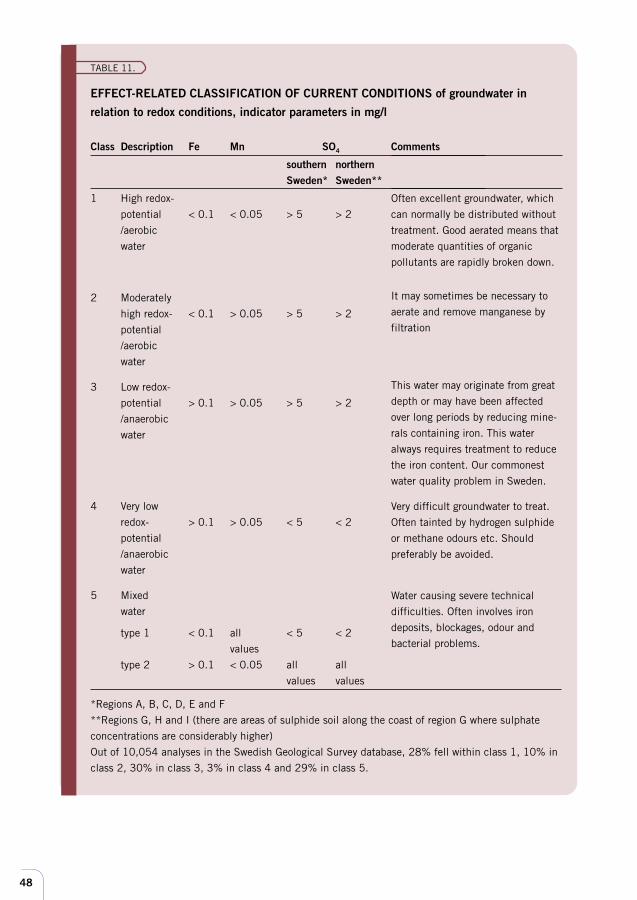
48

TABLE 11.

EFFECT-RELATED CLASSIFICATION OF CURRENT CONDITIONS of groundwater in

relation to redox conditions, indicator parameters in mg/l

Class Description Fe Mn SO4

southern northernSweden* Sweden**

1 High redox-

potential < 0.1 < 0.05 > 5 > 2

/aerobic

water

2 Moderately

high redox- < 0.1 > 0.05 > 5 > 2

potential

/aerobic

water

3 Low redox-

potential > 0.1 > 0.05 > 5 > 2

/anaerobic

water

4 Very low

redox- > 0.1 > 0.05 < 5 < 2

potential

/anaerobic

water

5 Mixed

water

type 1 < 0.1 all < 5 < 2

values

type 2 > 0.1 < 0.05 all all

values values

Comments

Often excellent groundwater, which

can normally be distributed without

treatment. Good aerated means that

moderate quantities of organic

pollutants are rapidly broken down.

It may sometimes be necessary to

aerate and remove manganese by

filtration

This water may originate from great

depth or may have been affected

over long periods by reducing mine-

rals containing iron. This water

always requires treatment to reduce

the iron content. Our commonest

water quality problem in Sweden.

Very difficult groundwater to treat.

Often tainted by hydrogen sulphide

or methane odours etc. Should

preferably be avoided.

Water causing severe technical

difficulties. Often involves iron

deposits, blockages, odour and

bacterial problems.

*Regions A, B, C, D, E and F

**Regions G, H and I (there are areas of sulphide soil along the coast of region G where sulphate

concentrations are considerably higher)

Out of 10,054 analyses in the Swedish Geological Survey database, 28% fell within class 1, 10% in

class 2, 30% in class 3, 3% in class 4 and 29% in class 5.

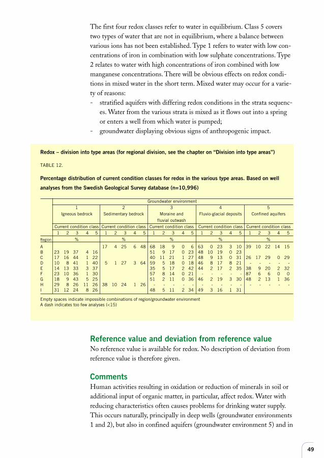
49

The first four redox classes refer to water in equilibrium. Class 5 coverstwo types of water that are not in equilibrium, where a balance betweenvarious ions has not been established. Type 1 refers to water with low con-centrations of iron in combination with low sulphate concentrations. Type2 relates to water with high concentrations of iron combined with lowmanganese concentrations. There will be obvious effects on redox condi-tions in mixed water in the short term. Mixed water may occur for a varie-ty of reasons:- stratified aquifers with differing redox conditions in the strata sequenc-

es. Water from the various strata is mixed as it flows out into a springor enters a well from which water is pumped;

- groundwater displaying obvious signs of anthropogenic impact.

Redox – division into type areas (for regional division, see the chapter on “Division into type areas”)

TABLE 12.

Percentage distribution of current condition classes for redox in the various type areas. Based on well

analyses from the Swedish Geological Survey database (n=10,996)




Region % % % % %

A 17 4 25 6 48 68 18 9 0 6 63 0 23 3 10 39 10 22 14 15B 23 19 37 4 16 51 9 17 0 23 48 10 19 0 23C 17 16 44 1 22 40 11 21 1 27 48 9 13 0 31 26 17 29 0 29D 10 8 41 1 40 5 1 27 3 64 59 5 18 0 18 46 8 17 8 21 - - - - -E 14 13 33 3 37 35 5 17 2 42 44 2 17 2 35 38 9 20 2 32F 23 10 36 1 30 57 8 14 0 21 - - - - - 87 6 6 0 0G 18 9 43 5 25 51 2 11 0 36 46 2 19 3 30 48 2 13 1 36H 29 8 26 11 26 38 10 24 1 26 - - - - - - - - - - - - - - -I 31 12 24 8 26 48 5 11 2 34 49 3 16 1 31


Reference value and deviation from reference valueNo reference value is available for redox. No description of deviation fromreference value is therefore given.

CommentsHuman activities resulting in oxidation or reduction of minerals in soil oradditional input of organic matter, in particular, affect redox. Water withreducing characteristics often causes problems for drinking water supply.This occurs naturally, principally in deep wells (groundwater environments1 and 2), but also in confined aquifers (groundwater environment 5) and in

50

association with areas of peat in other groundwater environments. Water-logging and compaction of ground, which prevent oxygen exchange be-tween the atmosphere and groundwater may also cause reducing condi-tions. An important consideration is that redox reactions often occur whenwater of one quality and origin is mixed with water of another. If disturb-ance ceases, the unstable waters will eventually assume a new chemicalthermodynamic equilibrium. Access to early monitoring series will then beneeded in order to analyse whether the waters were previously of a differ-ent quality. Thus, to identify anthropogenic impact, it will be necessary tohave several water samples taken on different occasions and to be able toestablish a change over time. Annual fluctuations in the water table them-selves cause changes in redox conditions, which has a bearing on sampling(see Appendix 1, page 77).

How can changes in redox be interpreted?A number of common causes of changes in redox conditions are given inthe examples below.• A change from class 1 to class 2 (elevated manganese concentrations) isoften a sign of shoreline infiltration. Abstraction of excessive quantities ofgroundwater has changed the direction of flow and induces infiltration ofsurface water at the shoreline, where groundwater previously seeped out.• A change from class 2 to class 3 or from class 3 to class 4 may have manycauses, but the disturbance is stable and a new thermodynamic equilibriumhas been established. One reason may be a lowering of the water tablecaused by pumping or drainage. A former outflow area has been transfor-med into an area where groundwater accumulates. Peat or other soils witha high organic content are often found here. Organic matter, which causesmore reducing conditions, may also originate from clear-cut areas, leakagefrom sewage infiltration plants or from areas where large quantities offarmyard manure are spread. Another cause of change may be abstractionduring dry periods. This may set stagnant groundwater in motion. Thistype of water, which has remained in an aquifer for a long time, is oftenanaerobic and iron-rich.• Changes class 1, 2 3 or 4 to class 5 indicate mixing of water of differingorigin. The commonest causes of this are changes in flow direction. Thismay occur naturally or as a consequence of human activities. Examples ofthe latter are groundwater abstraction and drainage.• Changes from a higher to a lower class, which lead to more oxidising con-ditions, may be due to discharges of nitrate. This impact may be local(most likely in igneous and metamorphic rock and moraine) or widespread(more common in sedimentary bedrock, fluvio-glacial material and inconfined aquifers). A reduction in the organic pollution load on ground-water may also create better oxidising conditions.

51

Assessment of concentrations of cadmium, zinc, lead and arsenic

IntroductionThis chapter deals with cadmium, zinc, lead and arsenic (a metalloid). Theyhave been selected because the concentrations recorded are often the resultof anthropogenic impact. Arsenic is not included in the EnvironmentalMonitoring Handbook and very few samples have yet been taken. Ourknowledge of the occurrence of arsenic has improved and a more criticalview of its health effects has been adopted in recent years.

These metals are usually present in such low concentrations in mineralsthat their concentration in water is limited by adsorption to humus, to ironand aluminium oxides/hydroxides and to minerals in clay. Some rocks, suchas schists, contain elevated concentrations, which may result in naturallyhigh concentrations in groundwater. Mineralisation in bedrock often con-sists of sulphides, which may be oxidised if the water table is loweredfollowing water abstraction. This will increase the risk of elevated metalconcentrations.

Metals entering groundwater from anthropogenic sourcesElevated metal concentrations often derive from anthropogenic sources suchas waste tips, mine spoil heaps and other industrial activities. The threemetals cadmium, zinc and lead are in common use. They are dispersed byemissions to air and soil and reach the groundwater. Cadmium is beingphased out in the manufacturing of products but has accumulated in agri-cultural soils and contaminated land. Zinc is much used in galvanised steelproducts, which often form part of ground-based constructions. Lead hasaccumulated in the ground as a result of exhaust emissions from vehiclesrunning on leaded petrol and also comes from buried lead-covered cables.Lead disperses within a few centimetres of these cables. All three metals be-come mobile in soil where pH levels are low, lead less so than the other two.

Wood preservatives for outdoor use contain arsenic. Leakage into theground and leaching from landfill sites threaten groundwater. Arsenic oc-curs as a negatively charged ion; its solubility is largely determined by redoxconditions and pH (see the chapter on “Redox”).

Metals

52

Metals having little anthropogenic impact on groundwaterIn Sweden, mercury, copper and aluminium are present in very low con-centrations in drinking water and are thus not described in detail here.Regarding the anthropogenically elevated concentrations that nonethelessdo occur, see the report on contaminated sites.

Occurrence and characteristicsCadmiumCadmium is stored in certain rocks, such as schists. In mineral form, cad-mium is often found in combination with zinc. Zinc is essential to mostorganisms and is actively absorbed by plants as well as animals. This meansthat cadmium, which is chemically very similar to zinc, is also easilyabsorbed. Cadmium concentrations are normally less than one 100th ofthose of zinc and organisms are unable to distinguish between the two.People suffering from iron deficiency may absorb cadmium instead of iron(Vahter, 1994). Cadmium is toxic at low concentrations and, as far as weknow, has no function in organisms. Cadmium is adsorbed to humus andminerals in clay. It is fairly weakly fixed in soil and is released at low pHwhen competition with hydrogen and aluminium ions increases. It hasbeen found that the concentration of cadmium rises rapidly in water, insoil and in groundwater at pH levels below 5. Hence, acidification involvesa risk of elevated cadmium concentrations.

ZincZinc is essential to most organisms and certainly to man. It is more harm-ful to aquatic organisms, however. Moderate concentrations of zinc ingroundwater are an indication of the presence of other metals, particularlycadmium. At most, cadmium concentrations reach one per cent of those ofzinc. Thus, 0.5 mg Zn/l may be accompanied by 5 µg Cd/l. Cadmiumoccurs with zinc in zinc ores and is also present in small quantities in gal-vanised coatings. Steel is often coated with a surface layer of zinc, chromi-um or nickel. Zinc is adsorbed to humic matter. It is liberated at low pHby competition from hydrogen and aluminium ions. Acidification there-fore involves a risk of elevated zinc concentrations in groundwater.

LeadThe average concentration of lead in the earth’s crust is 16 mg/kg; concen-trations in soil are somewhat higher. Lead is immobile in the soil environ-ment, since it adsorbs tightly to humus and minerals in clay. Lead is set inmotion at low pH levels and elevated concentrations of dissolved organicmatter. Adsorbed lead then enters the water attached to small suspendedparticles. Lead is non-essential to organisms. Acute lead poisoning affectshaemoglobin synthesis, which leads to iron deficiency. When pregnant

53

women are exposed to even moderate quantities of lead, the foetus maysuffer mental retardation (at concentrations above 10 µg/l). Metallic leadin direct contact with water is soluble in quantities that may easily exceedthe health-related limit value.

ArsenicArsenic exhibits moderate acute toxicity, but ingestion via water over along period even of quantities below the health-related limit value(50 µg/l) causes skin damage. Arsenic occurs in bedrock in combinationwith sulphides. It is mobilised in two main ways. Oxidation of sulphidesfollowing a lowering of the water table is one. The other results from thereduction of iron when arsenic is adsorbed to iron hydroxides. Reductionoften follows a rise in the water table. The risk of dissolved arsenic in theform of trivalent or pentavalent negatively charged ions, is greatest in cur-rent conditions class 3 according to Table 11 (”Redox” chapter). Concen-trations in groundwater may increase as pH rises, since adsorption to ironhydroxides is greatest in acid conditions. Adsorption declines as pH risesand arsenic is mobilised. Dissolved iron in groundwater may be an indica-tion of an elevated concentration of arsenic. Elevated iron concentrationsfrequently occur in water in deep wells bored in rock and there is reason tobelieve that arsenic may follow a similar pattern (Idman, 1996).

CopperCopper concentrations in groundwater are very low. The median figure ingroundwater in the Swedish Geological Survey database is around 1 µg/land the 90th percentile lies at about 5 µg/l. This means that 90 per cent ofall samples in Sweden have concentrations below 5 µg/l. Elevated copperconcentrations in drinking water occur as a result of corrosion of copperpipes. The National Food Administration health-related limit value is2,000 µg/l. A study based on 900 analyses revealed a median value forcopper in tap water standing overnight in pipes of 1,300 µg/l (Aastrup etal., 1995 and Figure 3, Appendix 10). Thus, copper in drinking water is acorrosion problem and is not therefore dealt with in further detail in thisreport.

AluminiumMany analyses reporting aluminium concentrations in groundwater areunreliable because the samples have not undergone proper filtration. Theconcentration of aluminium in groundwater is directly linked to pH. Dis-solved aluminium in groundwater seldom exceeds 100 µg/l at pH >5.5.When weathering of carbonate and feldspar is no longer sufficient to actas a buffer, aluminium begins to do so. The high content of aluminium inminerals in the soil provides a buffer for acid water with a pH below 5.

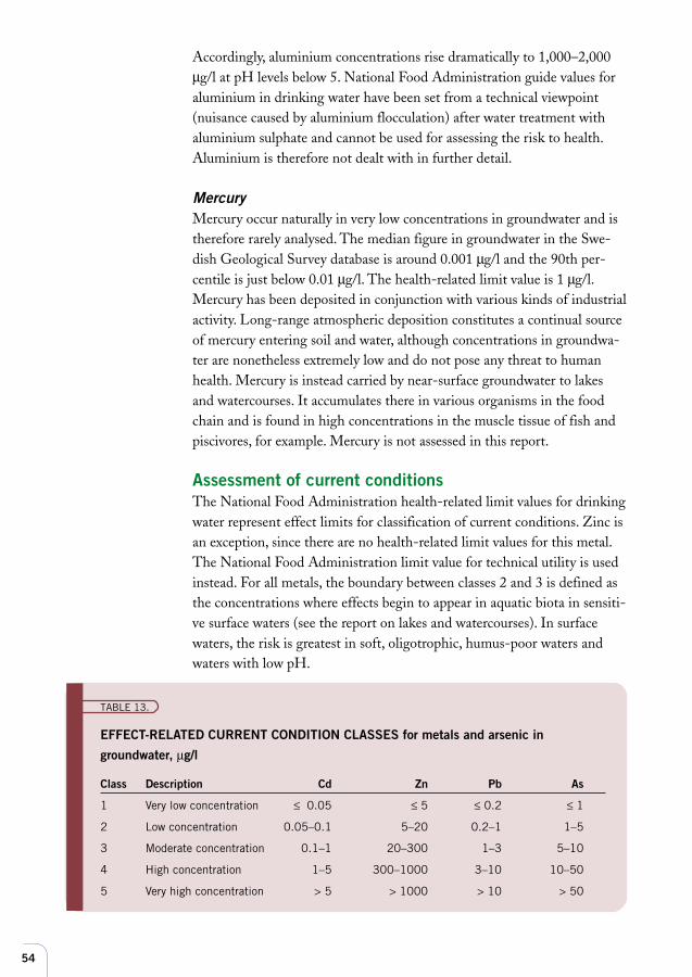
54

Accordingly, aluminium concentrations rise dramatically to 1,000–2,000µg/l at pH levels below 5. National Food Administration guide values foraluminium in drinking water have been set from a technical viewpoint(nuisance caused by aluminium flocculation) after water treatment withaluminium sulphate and cannot be used for assessing the risk to health.Aluminium is therefore not dealt with in further detail.

MercuryMercury occur naturally in very low concentrations in groundwater and istherefore rarely analysed. The median figure in groundwater in the Swe-dish Geological Survey database is around 0.001 µg/l and the 90th per-centile is just below 0.01 µg/l. The health-related limit value is 1 µg/l.Mercury has been deposited in conjunction with various kinds of industrialactivity. Long-range atmospheric deposition constitutes a continual sourceof mercury entering soil and water, although concentrations in groundwa-ter are nonetheless extremely low and do not pose any threat to humanhealth. Mercury is instead carried by near-surface groundwater to lakesand watercourses. It accumulates there in various organisms in the foodchain and is found in high concentrations in the muscle tissue of fish andpiscivores, for example. Mercury is not assessed in this report.

Assessment of current conditionsThe National Food Administration health-related limit values for drinkingwater represent effect limits for classification of current conditions. Zinc isan exception, since there are no health-related limit values for this metal.The National Food Administration limit value for technical utility is usedinstead. For all metals, the boundary between classes 2 and 3 is defined asthe concentrations where effects begin to appear in aquatic biota in sensiti-ve surface waters (see the report on lakes and watercourses). In surfacewaters, the risk is greatest in soft, oligotrophic, humus-poor waters andwaters with low pH.

TABLE 13.

EFFECT-RELATED CURRENT CONDITION CLASSES for metals and arsenic in

groundwater, µg/l

Class Description Cd Zn Pb As

1 Very low concentration ≤ 0.05 ≤ 5 ≤ 0.2 ≤ 1

2 Low concentration 0.05–0.1 5–20 0.2–1 1–5

3 Moderate concentration 0.1–1 20–300 1–3 5–10

4 High concentration 1–5 300–1000 3–10 10–50

5 Very high concentration > 5 > 1000 > 10 > 50

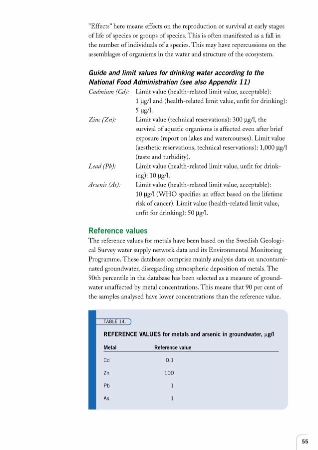
55

”Effects” here means effects on the reproduction or survival at early stagesof life of species or groups of species. This is often manifested as a fall inthe number of individuals of a species. This may have repercussions on theassemblages of organisms in the water and structure of the ecosystem.

Guide and limit values for drinking water according to theNational Food Administration (see also Appendix 11)Cadmium (Cd): Limit value (health-related limit value, acceptable):

1 µg/l and (health-related limit value, unfit for drinking):5 µg/l.

Zinc (Zn): Limit value (technical reservations): 300 µg/l, thesurvival of aquatic organisms is affected even after briefexposure (report on lakes and watercourses). Limit value(aesthetic reservations, technical reservations): 1,000 µg/l(taste and turbidity).

Lead (Pb): Limit value (health-related limit value, unfit for drink-ing): 10 µg/l.

Arsenic (As): Limit value (health-related limit value, acceptable):10 µg/l (WHO specifies an effect based on the lifetimerisk of cancer). Limit value (health-related limit value,unfit for drinking): 50 µg/l.

Reference valuesThe reference values for metals have been based on the Swedish Geologi-cal Survey water supply network data and its Environmental MonitoringProgramme. These databases comprise mainly analysis data on uncontami-nated groundwater, disregarding atmospheric deposition of metals. The90th percentile in the database has been selected as a measure of ground-water unaffected by metal concentrations. This means that 90 per cent ofthe samples analysed have lower concentrations than the reference value.

TABLE 14.

REFERENCE VALUES for metals and arsenic in groundwater, µg/l

Metal Reference value

Cd 0.1

Zn 100

Pb 1

As 1

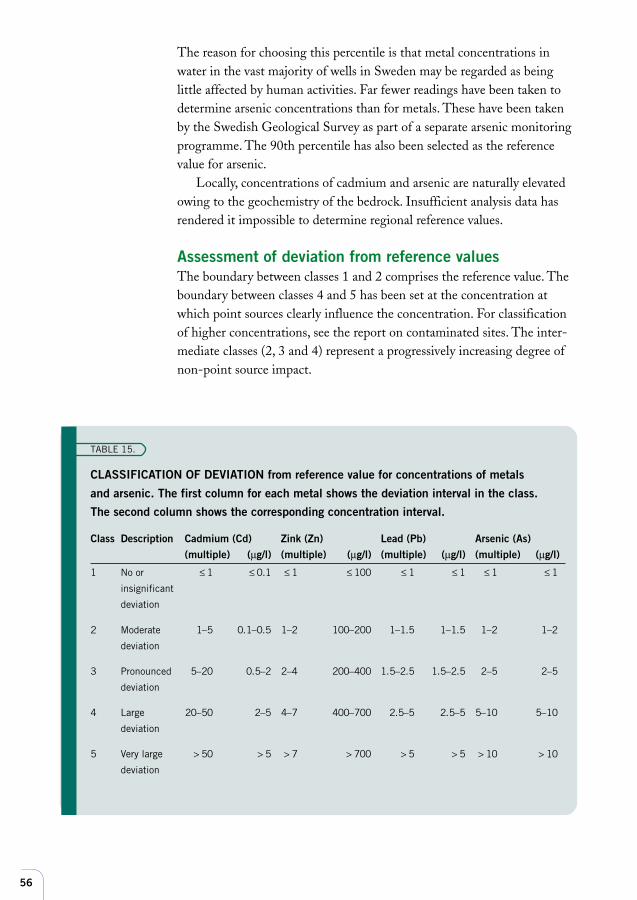
56

The reason for choosing this percentile is that metal concentrations inwater in the vast majority of wells in Sweden may be regarded as beinglittle affected by human activities. Far fewer readings have been taken todetermine arsenic concentrations than for metals. These have been takenby the Swedish Geological Survey as part of a separate arsenic monitoringprogramme. The 90th percentile has also been selected as the referencevalue for arsenic.

Locally, concentrations of cadmium and arsenic are naturally elevatedowing to the geochemistry of the bedrock. Insufficient analysis data hasrendered it impossible to determine regional reference values.

Assessment of deviation from reference valuesThe boundary between classes 1 and 2 comprises the reference value. Theboundary between classes 4 and 5 has been set at the concentration atwhich point sources clearly influence the concentration. For classificationof higher concentrations, see the report on contaminated sites. The inter-mediate classes (2, 3 and 4) represent a progressively increasing degree ofnon-point source impact.

TABLE 15.

CLASSIFICATION OF DEVIATION from reference value for concentrations of metals

and arsenic. The first column for each metal shows the deviation interval in the class.

The second column shows the corresponding concentration interval.

Class Description Cadmium (Cd) Zink (Zn) Lead (Pb) Arsenic (As)(multiple) (µg/l) (multiple) (µg/l) (multiple) (µg/l) (multiple) (µg/l)

1 No or ≤ 1 ≤ 0.1 ≤ 1 ≤ 100 ≤ 1 ≤ 1 ≤ 1 ≤ 1

insignificant

deviation

2 Moderate 1–5 0.1–0.5 1–2 100–200 1–1.5 1–1.5 1–2 1–2

deviation

3 Pronounced 5–20 0.5–2 2–4 200–400 1.5–2.5 1.5–2.5 2–5 2–5

deviation

4 Large 20–50 2–5 4–7 400–700 2.5–5 2.5–5 5–10 5–10

deviation

5 Very large > 50 > 5 > 7 > 700 > 5 > 5 > 10 > 10

deviation

57

Dispersal, impact and concentration in groundwaterof metalsCadmiumNaturally high concentrations of cadmium occur in some regions of thecountry with sedimentary bedrock even where pH is not particularly low.Cadmium is stored here in certain rocks, such as shales. Where alum shaleis a pronounced feature in the soil, this may cause elevated concentrationsof cadmium in groundwater.

Cadmium enters soils via long-range dispersal and from point sources.Long-range dispersal has been in the form of atmospheric deposition(originating from, eg, engineering plants and zinc manufacture) andfollowing use of phosphate fertilisers. Although these emissions have de-creased, much cadmium remains fixed in organic matter in the soil. Inparticular, cadmium has accumulated in forest and agricultural soils insouthern Sweden. In places, the quantity of fixed cadmium in agriculturalsoils has almost doubled over the last fifty years.

Examples of point sources include smelting works and nickel-cadmiumbattery factories. This impact may extend up to ten kilometres from thesource. Fossil fuel burning may also cause locally elevated cadmium con-centrations. Where concentrations exceed 5 µg/l and the groundwater isnot extremely acid, there is every reason to suspect emissions from a localsource. If the area is not underlain by sedimentary bedrock and the pH isover 5, concentrations above 0.5 µg/l will quite definitely indicate an an-thropogenic source. A number of mechanisms may act in concert to causeelevated concentrations in the range 0.5–5 µg/l.

ZincThe main sources of elevated zinc concentrations, even where pH is notparticularly low, are ore mining spoil heaps.

Galvanised (zinc coated) materials are used for innumerable applica-tions. Since zinc may dissolve when metals corrode, it is found in elevatedconcentrations in many soil environments. Landfill sites usually containlarge quantities of galvanised material and it is common to find elevatedzinc concentrations in leachate. Zinc is used for many other purposes,including feed for newly born piglets, and it thus immediately enters thesoil. Zinc has also been used in wood preservatives and may therefore bepresent in soil and water in the vicinity of old impregnation plants.

Where concentrations exceed 700 µg/l in groundwater, there is reasonto suspect a local pollution source. A number of mechanisms may act to-gether to mobilise zinc and raise levels of this metal at lower concentrationranges.

58

LeadThe main source of lead dispersal is now its use in accumulators. Anothermajor source is leaching from spoil heaps. Sulphide ore waste may have a leadcontent of about one tenth of a per cent. Leaching from this is moderatecompared with that of zinc and cadmium because lead is more tightly adsor-bed to the material than the other two. Lead has also been dispersed in theenvironment by emissions to air from smelting works, by use in batteries, inammunition and, formerly, as a petrol additive. Lead concentrations alongmost roads are elevated by a multiple of 10–20. Embankments at shootingranges may contain several per cent lead, which may then disperse into thegroundwater in the absence of organic matter or other effective adsorbents.

ArsenicNaturally high concentrations of arsenic in groundwater are found at a fewlocations on the Skellefteå plain in northern Sweden and in Bergslagen incentral Sweden. Sulphide ores, particular those from the northern province ofVästerbotten, contain high concentrations of this element, as do shales in thesame area. Water from deep wells with high iron concentrations and accom-panying high pH in other parts of the country may also exhibit elevated arse-nic concentrations (above 10µg/l).

Arsenic is used as a wood preservative (Cu-Cr-As impregnation) andgroundwater at impregnation plants often displays elevated concentrations ofarsenic. Landfill sites will probably be a future source of arsenic in groundwa-ter, when the large quantities of CCA-impregnated timber currently in use arelandfilled.

If samples come from areas other than those mentioned above and thewater does not fit into redox class 3 (see the chapter on “Redox”, Table 11),concentrations over 10 µg/l are quite definitely caused by a point source.

ReferencesAastrup, M., Berntell, A., Bertills, U., Johnson, J. & Thunholm, B. (1995): Ground-

water chemistry in Sweden. – Swedish Environmental Protection Agency Report

4416.

Idman, H. (1996): Naturally occurring arsenic in groundwaters and factors affecting its

concentration. Nystén, T., Suokko, T. & Tarvainen, T. (Eds.) In environmental geology

seminar in Helsinki, 1 Oct. 1996. – Report 71 published by the Finnish Environmen-

tal Agency, pp 17–22.

Vahter, M. & Lind, B. (1986): Concentration of arsenic in urine of the general popula-

tion in Sweden. Sci. Total Environ. 54:1-12.

WHO Guidelines for drinking water quality. Second ed. Vol. 1 Recommendations.

– WHO Geneva, 1993.

59

This chapter is arranged as a classification of risk for pesticide contamina-

tion of groundwater

IntroductionThe greatest quantities of pesticides are used in the forest products indus-try. Other use primarily occurs in agriculture, where weedkillers predomi-nate, followed by fungicides, insecticides and agents to combat mites. Lar-ge quantities are also used in private gardens, in market gardening, on golfcourses, sports grounds, railway embankments, roadside verges and hardsurfaces. Forestry accounts for a fairly small proportion of pesticide use.Agricultural pesticides are often based on organic compounds, which arescarcely soluble in water. In some circumstances, they can permeate soiland reach the groundwater. Once down in the groundwater zone, they canmove on to areas “downstream” and end up in surface or well water farfrom the place they were used. The forest products industry uses woodpreservatives containing easily soluble metal salts to treat timber againstfungal attack. These are dealt with further in the chapter on “Metals”.

Model for risk classificationA procedure for classifying soil areas according to risk makes it easier toplan studies into the presence of pesticides in groundwater. Sampling andanalysis can then focus on the areas with the greatest risk of pollution.This is important, since analysis of pesticides in groundwater is expensive.

• Risk classification relates both to normal dispersal and to other use ofpesticides.

• Risk classification relates both to agricultural land and to land used forother purposes. Considerable quantities are used in gardens, although it isoften difficult to determine the extent of this use. The approach to theseareas must be decided on the merits of each case.

• Risk classification is intended to serve as a model taking account of indi-vidual factors of particular importance. These risk factors have been classi-

Pesticides

60

fied according to a five-point scale. The specific conditions are evaluatedand the individual factors are then weighed up to arrive at a final riskclassification.

Recommended samplingA selection of pesticides has been made so as to focus on substances poten-tially able to leach out of soil, those that have been detected in ground-water and/or those that are used in large quantities. These are presented inAppendix 7. The limited number of pesticides proposed for inclusion in aninitial analysis package by no means covers all those currently in use inSweden and their metabolites (products of decomposition). The proposalshould be seen as a compromise made to reduce the cost of analysis, there-by allowing analysis of a greater number of water supply sources. For somewater supplies, there may be reason to include other pesticides used locallyin large quantities, eg, those used in bulk in potato cultivation. It is there-fore important to be aware of pesticides used locally in large quantities butnot included in the list in Appendix 7. This list includes certain agentsrequiring specific analytical methods. Different laboratories may havediffering “pesticide packages”. It is important to consult the laboratorybefore ordering analyses. If samples repeatedly indicate the presence ofpesticides or if more than one pesticide is found at the same time, it isproposed that the analysis package be expanded. It should also be borne inmind that a negative result from the analysis of a limited number of pesti-cides does not necessarily indicate that the water is free of pesticides.

The EC drinking water directive threshold for remedial action is 0.1µg/l for each individual pesticide and 0.5 µg/l for total pesticides.

Risk classificationA risk assessment is made in areas where spraying takes place or has takenplace. The factors considered of most importance to whether pesticidesmay migrate into the groundwater are listed in Tables 16 and 17. Theserisk factors have been classified according to a five-point scale, from a to e,where a represents the least risk and e the greatest. The letters representingthe risk factors in the area to be assessed are entered in the column headed“Assessment area”. When both tables have been completed, the individualrisk factors can be weighed up using Table 18, which will give the relevantrisk class. Sampling is recommended for areas falling within class 3.

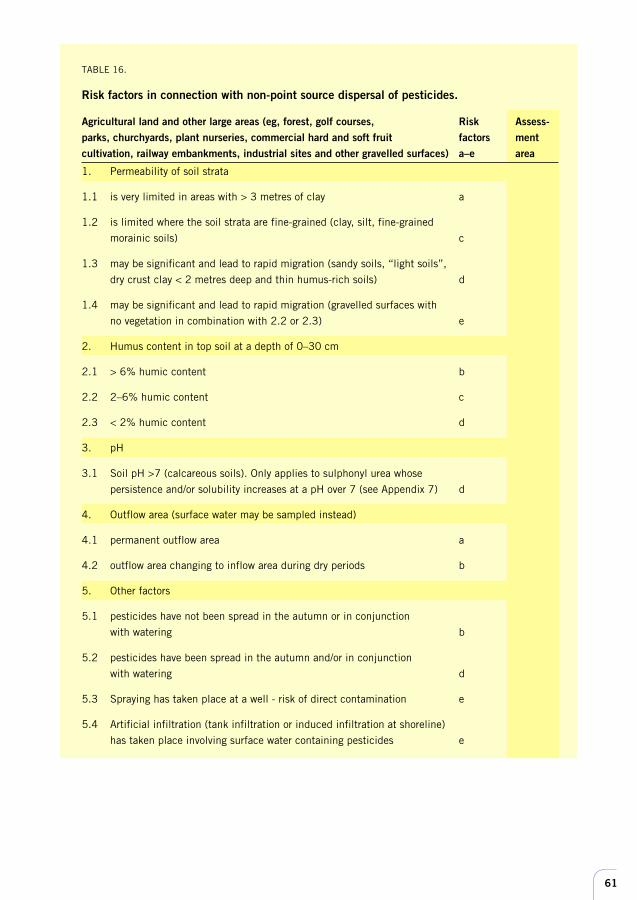
61

TABLE 16.

Risk factors in connection with non-point source dispersal of pesticides.

Agricultural land and other large areas (eg, forest, golf courses, Risk Assess-parks, churchyards, plant nurseries, commercial hard and soft fruit factors mentcultivation, railway embankments, industrial sites and other gravelled surfaces) a–e area

1. Permeability of soil strata

1.1 is very limited in areas with > 3 metres of clay a

1.2 is limited where the soil strata are fine-grained (clay, silt, fine-grained

morainic soils) c

1.3 may be significant and lead to rapid migration (sandy soils, “light soils”,

dry crust clay < 2 metres deep and thin humus-rich soils) d

1.4 may be significant and lead to rapid migration (gravelled surfaces with

no vegetation in combination with 2.2 or 2.3) e

2. Humus content in top soil at a depth of 0–30 cm

2.1 > 6% humic content b

2.2 2–6% humic content c

2.3 < 2% humic content d

3. pH

3.1 Soil pH >7 (calcareous soils). Only applies to sulphonyl urea whose

persistence and/or solubility increases at a pH over 7 (see Appendix 7) d

4. Outflow area (surface water may be sampled instead)

4.1 permanent outflow area a

4.2 outflow area changing to inflow area during dry periods b

5. Other factors

5.1 pesticides have not been spread in the autumn or in conjunction

with watering b

5.2 pesticides have been spread in the autumn and/or in conjunction

with watering d

5.3 Spraying has taken place at a well - risk of direct contamination e

5.4 Artificial infiltration (tank infiltration or induced infiltration at shoreline)

has taken place involving surface water containing pesticides e

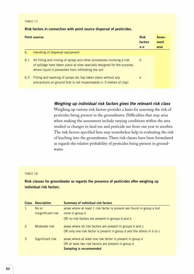
62

Weighing up individual risk factors gives the relevant risk classWeighing up various risk factors provides a basis for assessing the risk ofpesticides being present in the groundwater. Difficulties that may arisewhen making the assessment include varying conditions within the areastudied or changes in land use and pesticide use from one year to another.The risk factors specified here may nonetheless help in evaluating the riskof leaching into the groundwater. Three risk classes have been formulatedas regards the relative probability of pesticides being present in ground-water.

TABLE 17.

Risk factors in connection with point source dispersal of pesticides.

Point sources Risk Asses-factors menta–e area

6. Handling of dispersal equipment

6.1 All filling and rinsing of sprays and other procedures involving a risk b

of spillage have taken place at sites specially designed for the purpose,

where liquid is prevented from infiltrating the soil

6.2 Filling and washing of sprays etc has taken place without any e

precautions on ground that is not impermeable (< 3 metres of clay)

TABLE 18.

Risk classes for groundwater as regards the presence of pesticides after weighing up

individual risk factors.

Class Description Summary of individual risk factors

1 No or areas where at least 1 risk factor is present are found in group a but

insignificant risk none in group e

OR no risk factors are present in groups d and e

2 Moderate risk areas where all risk factors are present in groups b and c

OR only one risk factor is present in group d and the others in b or c

3 Significant risk areas where at least one risk factor is present in group e

OR at least two risk factors are present in group d

Sampling is recommended

63

Indirect risk – dispersal of pesticides via groundwater toother areasA list is given below of conditions of importance when evaluating risks inareas “downstream” of class 3 areas. These may be areas of land wherepesticides have never been used. The far boundary of areas that may havebeen affected is very difficult to determine but will generally be limited bythe outflow area. Beyond this, pesticides may be present in surface waterinstead. Although several of these conditions are difficult to assess, theyshould be evaluated where applicable.• the number of years pesticides have been used or analysed in the

groundwater• the size of the areas sprayed• geological conditions for major variations in the rate of groundwater

flow within the area (see page 33 of the report on contaminated sitesfor help in assessing this factor)

• hydrogeological conditions appropriate for a high or a low degree offixing, dilution and decomposition within the area.

ReferencesEC groundwater and drinking water directives. Dir. 80/68/EEC and Dir. 80/778/

EEC.

Hessel, K., Kreuger, J. & Ulén, B. (1997): Kartläggning av bekämpningsmedelsres-

ter i yt-, grund- och regnvatten i Sverige 1985–1995. Resultat från monitoring och

riktad provtagning. (”Survey of pesticide residues in surface water, groundwater

and rain water in Sweden 1985–1995. Results of monitoring and concentrated

sampling”) – Ekohydrologi 42, Swedish University of Agricultural Sciences, De-

partment of Water Management, Uppsala.

National Food Administration drinking water regulations, SLV FS 1993:35.

Maxe, L. & Johansson, P.-O. (1998): Bedömning av grundvattens sårbarhet –

Utvecklingsmöjligheter (”Assessment of groundwater sensitivity – Scope for deve-

lopment”). In Swedish – Swedish Environmental Protection Agency Report 4852.

Swedish EPA (1993): Kemiska bekämpningsmedel i den yttre miljön (”Pesticides

in the environment”) – Swedish Environmental Protection Agency Informs.

Swedish EPA (1997): Spridning av kemiska bekämpningsmedel. Tillämpning av

Naturvårdsverkets föreskrifter om spridning av kemiska bekämpningsmedel (”Dis-

persal of pesticides. Application of Swedish Environmental Protection Agency

regulations on pesticide dispersal”) – General Guidelines 97:3.

64

Assessment of deviation from the natural seasonal variations in the water

table. The Swedish Geological Survey’s monthly maps of water table status

throughout the country, seasonal graphs of fluctuations in the water table

and local reference series are used.

IntroductionChanges in the (pressure) level of the water table can cause problems ofvarious kinds. Common problems caused by low levels include:• water shortages in groundwater supplies from wells as well as from

natural springs• salt salt water intrusion in wells in coastal areas or areas where relict sea

water is present• oxidation of sulphurous soils, resulting in acidification problems• land subsidence in certain fine grained cohesive soils• risk of high iron and manganese concentrations due to drainage of

discharge areas• drying up of the soil surface causing biotope changes in wetland areas

Problems caused by high levels include:• increasing risk of deterioration in water quality, e.g., in the form of

high iron and manganese concentrations• land slip and poor ultimate bearing resistance• waterlogging and increased concentrations of organic matter in the

groundwater

Human activities which may affect the water table:• groundwater abstraction and changes in abstraction (wells)• regulation of watercourses• drainage and excavation below the water table (drainage resulting from

underground construction, tunnels, underground cavities or deep foun-dations involving pumping of groundwater)

• prevention of groundwater formation (as a result of ground surfacing inurban areas and rerouting of storm water)

Water table

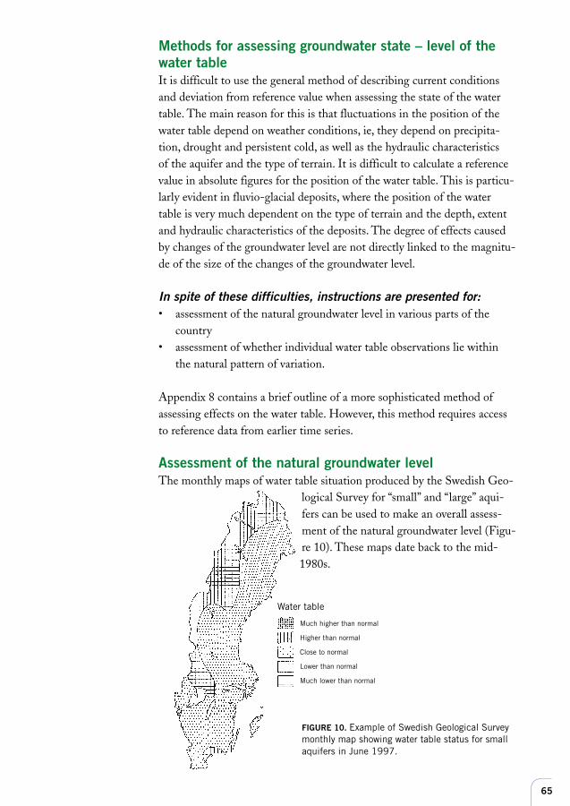
65

Methods for assessing groundwater state – level of thewater tableIt is difficult to use the general method of describing current conditionsand deviation from reference value when assessing the state of the watertable. The main reason for this is that fluctuations in the position of thewater table depend on weather conditions, ie, they depend on precipita-tion, drought and persistent cold, as well as the hydraulic characteristicsof the aquifer and the type of terrain. It is difficult to calculate a referencevalue in absolute figures for the position of the water table. This is particu-larly evident in fluvio-glacial deposits, where the position of the watertable is very much dependent on the type of terrain and the depth, extentand hydraulic characteristics of the deposits. The degree of effects causedby changes of the groundwater level are not directly linked to the magnitu-de of the size of the changes of the groundwater level.

In spite of these difficulties, instructions are presented for:• assessment of the natural groundwater level in various parts of the

country• assessment of whether individual water table observations lie within

the natural pattern of variation.

Appendix 8 contains a brief outline of a more sophisticated method ofassessing effects on the water table. However, this method requires accessto reference data from earlier time series.

Assessment of the natural groundwater levelThe monthly maps of water table situation produced by the Swedish Geo-

logical Survey for “small” and “large” aqui-fers can be used to make an overall assess-ment of the natural groundwater level (Figu-re 10). These maps date back to the mid-1980s.

FIGURE 10. Example of Swedish Geological Surveymonthly map showing water table status for smallaquifers in June 1997.

Much higher than normal

Higher than normal

Close to normal

Lower than normal

Much lower than normal

Water table

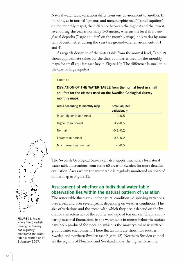
66

TABLE 19.

DEVIATION OF THE WATER TABLE from the normal level in small

aquifers for the classes used on the Swedish Geological Survey

monthly maps.

Class according to monthly map Small aquiferdeviation, m

Much higher than normal > 0.5

Higher than normal 0.2–0.5

Normal -0.2–0.2

Lower than normal -0.5–0.2

Much lower than normal < -0.5

FIGURE 11. Areaswhere the SwedishGeological Surveyhas regularlymonitored the watertable elevation as of1 January 1997.

Natural water table variations differ from one environment to another. Inmoraine, as in normal “igneous and metamorphic rock” (”small aquifers”on the monthly maps), the difference between the highest and the lowestlevel during the year is normally 1–3 metres, whereas the level in fluvio-glacial deposits (”large aquifers” on the monthly maps) only varies by sometens of centimetres during the year (see groundwater environments 3, 1and 4).

As regards deviation of the water table from the normal level, Table 19shows approximate values for the class boundaries used for the monthlymaps for small aquifers (see key in Figure 10). The difference is smaller inthe case of large aquifers.

The Swedish Geological Survey can also supply time series for naturalwater table fluctuations from some 60 areas of Sweden for more detailedevaluation. Areas where the water table is regularly monitored are markedon the map in Figure 11.

Assessment of whether an individual water tableobservation lies within the natural pattern of variationThe water table fluctuates under natural conditions, displaying variationsover a year and over several years, depending on weather conditions. Thesize of variations and the speed with which they occur depend on the hy-draulic characteristics of the aquifer and type of terrain, etc. Graphs com-paring seasonal fluctuations in the water table in metres below the surfacehave been produced for moraine, which is the most typical near-surfacegroundwater environment. These fluctuations are shown for southernSweden and northern Sweden (see Figure 12). Northern Sweden compri-ses the regions of Norrland and Svealand above the highest coastline.

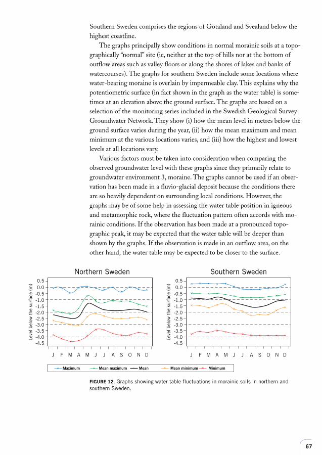
67

Southern Sweden comprises the regions of Götaland and Svealand below thehighest coastline.

The graphs principally show conditions in normal morainic soils at a topo-graphically “normal” site (ie, neither at the top of hills nor at the bottom ofoutflow areas such as valley floors or along the shores of lakes and banks ofwatercourses). The graphs for southern Sweden include some locations wherewater-bearing moraine is overlain by impermeable clay. This explains why thepotentiometric surface (in fact shown in the graph as the water table) is some-times at an elevation above the ground surface. The graphs are based on aselection of the monitoring series included in the Swedish Geological SurveyGroundwater Network. They show (i) how the mean level in metres below theground surface varies during the year, (ii) how the mean maximum and meanminimum at the various locations varies, and (iii) how the highest and lowestlevels at all locations vary.

Various factors must be taken into consideration when comparing theobserved groundwater level with these graphs since they primarily relate togroundwater environment 3, moraine. The graphs cannot be used if an obser-vation has been made in a fluvio-glacial deposit because the conditions thereare so heavily dependent on surrounding local conditions. However, thegraphs may be of some help in assessing the water table position in igneousand metamorphic rock, where the fluctuation pattern often accords with mo-rainic conditions. If the observation has been made at a pronounced topo-graphic peak, it may be expected that the water table will be deeper thanshown by the graphs. If the observation is made in an outflow area, on theother hand, the water table may be expected to be closer to the surface.

FIGURE 12. Graphs showing water table fluctuations in morainic soils in northern andsouthern Sweden.

J F M A M J J A S O N D

Norra Sverige

Niv

å un

der

mar

kyta

n (m

) 0,50,0

-0,5-1,0-1,5-2,0-2,5-3,0-3,5-4,0-4,5

Maximum Medelmax Medel Medelmin Minimum

J F M A M J J A S O N D

Södra Sverige

Niv

å un

der

mar

kyta

n (m

) 0,50,0

-0,5-1,0-1,5-2,0-2,5-3,0-3,5-4,0-4,5

Southern SwedenNorthern Sweden

Leve

l bel

ow t

he s

urfa

ce (

m)

Leve

l bel

ow t

he s

urfa

ce (

m)

0.50.0

-0.5-1.0-1.5-2.0-2.5-3.0-3.5-4.0-4.5

0.50.0

-0.5-1.0-1.5-2.0-2.5-3.0-3.5-4.0-4.5

Maximum Mean maximum Mean Mean minimum Minimum

68

The assessment must also take account of weather conditions duringthe period immediately preceding the observation. An observed low watertable during a dry period may very well be natural, whereas a low levelduring a year with heavy precipitation probably has an anthropogenic ex-planation. Hence, during a “wet” year, it should be expected that the posi-tion of the water table will be above the mean level shown in the graphs.During a dry year it will be below that level.

ReferencesGrip, H. & Rodhe, A. (1985): Vattens väg från regn till bäck (”Water – from rain

to stream”). – Research Council Publications, Karlshamn.

Swedish Geological Survey (1994): Grundvattnet i Sverige (”Swedish groundwa-

ter”). – SGU serie AH nr. 17.

Knutsson, G. & Morfeldt, C.-O. (1993): Grundvatten: teori och tillämpning

(”Groundwater – theory and practice”). – Svensk byggtjänst, Solna.

Nordberg, L. & Persson, G. (1979): Vårt vatten: tillgång, utnyttjande (”Our water:

supply and use”). – Stockholm.

69

Variation is a normal phenomenon in the environment and occurs in all

undisturbed ecosystems. This natural variation makes it more difficult to

determine the degree of anthropogenic impact. The deviation test presented

here makes it possible to compare the distribution of readings taken in a

type area with the distribution of all readings from the same type area in the

entire database. This in turn makes it possible to identify impacts origina-

ting from point sources.

Reference databaseA specific reference database has been compiled of all available ground-water analyses. In total, it comprises data from nearly 30,000 wells. Theanalyses are mainly from the 1980s. They have been performed by munici-palities, well borers, universities and government agencies and reflectgroundwater composition in the 1980s, including existing human impactin the form of acid precipitation and nitrogen contamination for example.Nonetheless, they provide a valuable indication of the natural variationwithin a population of groundwater samples, particularly since the materialhas been broken down into type areas.

Concentration distributions for the 36 type areas (subdivided as shownin Table 1 on page 27) are given in Tables 1–12 in Appendix 2. In thesetables, each type area is divided into two depth classes. When samples aretaken in the various type areas, the distribution of concentrations may beof help for assessment purposes.

Deviation testThe great natural variation in concentrations of various substances in wateroccurs because an aquifer is a heterogeneous medium. This causes a dis-persal of the concentrations of the various chemical constituents. Thesmaller the number of readings available for a given constituent in a giventype area, the more difficult it is to determine how representative they areof the type area in question. A deviation test has therefore been developedto determine whether or not samples deviate significantly from the con-centration distribution shown here.

Instructionsfor deviation test

70

The test is performed in the following stages:

(a) Group the analyses according to type areaThe groundwater samples taken are grouped according to type area andwell depth.

(b) Calculate a weighting index for the relevant parameter usingTables 1–12 in Appendix 2The readings obtained are compared and classified against the concentra-tion distributions for the corresponding type area and well-depth class inthe appendix. (Tables 1 –12 include the parameters assessed in this report.)

Values ≤ 5th percentile are given a class value of 1Values > 5th percentile and ≤ 25th percentile are given a class value of 2Values > 25th percentile and ≤ 75th percentile are given a class value of 3Values > 75th percentile and ≤ 95th percentile are given a class value of 4Values > 95th percentile are given a class value of 5

The weighting index is calculated as the mean of the class values obtained.The weighting index will always lie between 1 and 5. By definition, theweighting index of the reference population is always 3.

(c) Assess the weighting index obtainedIf the calculated weighting index for the parameter in question is 3, theconcentration distribution is the same (or very similar to) that of the refe-rence population. If, on the other hand, the index obtained deviates greatlyfrom 3, there is a difference between the concentration distribution obtai-ned and that of the reference population. If the value exceeds 3, the distri-bution is wider than that of the reference population. Below 3, the distri-bution obtained is below that of the reference population. The calculatedweighting index is compared with critical values in Table 13 in Appendix 2to determine whether it differs to a statistically significant extent. Thecritical values used in Appendix 2 depend on the number of samples in thepopulation to be compared and the choice of significance level (= risk thatthe difference obtained is random).

If there are five samples and these give a weighting index of 4.00, thiscan be interpreted to mean that the population being compared is signifi-cantly higher than the reference population at a significance of 5 per cent,but not at a significance of 1 per cent. (5 per cent often suffices. This me-ans that the risk of deviation being random is 5 per cent.) If, on the otherhand, the weighting index is 2.00, one can conclude by analogy that thepopulation being compared at the 5 per cent is lower than the referencepopulation but not at the 1 per cent level, which, it must be remembered,

71

requires a weighting index of less than 1.80 to be significant for five samp-les. If the population being compared contains more samples, significancewill be attained at a progressively falling weighting index. (The moresamples, the less the deviation from 3 needed to achieve significance.)

If a weighting index significantly deviates from the median of the refe-rence population (3), a more detailed analysis should be made of the rea-sons for this. Could it be due to natural causes such as unusual shallownessof the wells sampled or the presence of clay containing sulphide? Or is itdue to anthropogenic impact in the form of local waste tips, drainage orabstraction of excessive quantities of water from wells?

An example of the way a deviation test may be presented is given inAppendix 3.

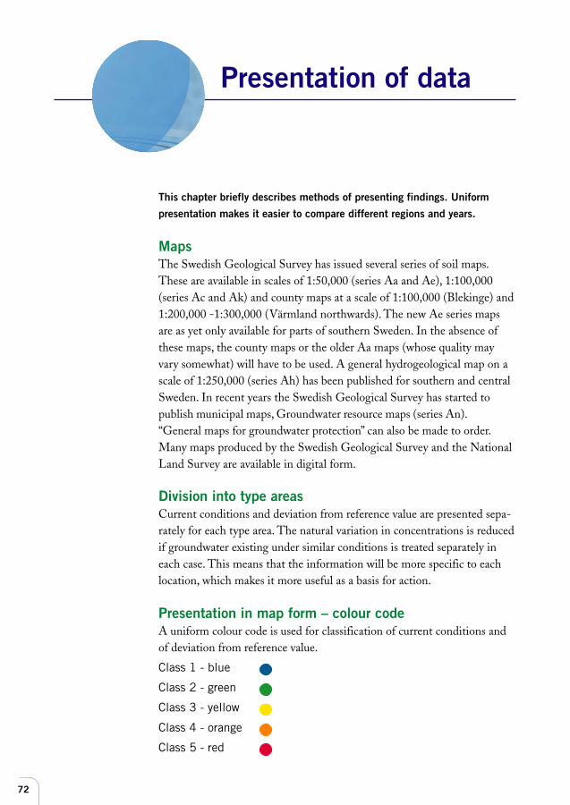
72

This chapter briefly describes methods of presenting findings. Uniform

presentation makes it easier to compare different regions and years.

MapsThe Swedish Geological Survey has issued several series of soil maps.These are available in scales of 1:50,000 (series Aa and Ae), 1:100,000(series Ac and Ak) and county maps at a scale of 1:100,000 (Blekinge) and1:200,000 -1:300,000 (Värmland northwards). The new Ae series mapsare as yet only available for parts of southern Sweden. In the absence ofthese maps, the county maps or the older Aa maps (whose quality mayvary somewhat) will have to be used. A general hydrogeological map on ascale of 1:250,000 (series Ah) has been published for southern and centralSweden. In recent years the Swedish Geological Survey has started topublish municipal maps, Groundwater resource maps (series An). “General maps for groundwater protection” can also be made to order.Many maps produced by the Swedish Geological Survey and the NationalLand Survey are available in digital form.

Division into type areasCurrent conditions and deviation from reference value are presented sepa-rately for each type area. The natural variation in concentrations is reducedif groundwater existing under similar conditions is treated separately ineach case. This means that the information will be more specific to eachlocation, which makes it more useful as a basis for action.

Presentation in map form – colour codeA uniform colour code is used for classification of current conditions andof deviation from reference value.

Class 1 - blue

Class 2 - green

Class 3 - yellow

Class 4 - orange

Class 5 - red

Presentation of data

73

If the material is printed in monochrome, classes can instead be identifiedusing numbers or be used in combination with suitable rasters.

Great caution should be exercised when extrapolating from samplepoints to whole areas of the map. Colouring of individual dots is preferableif little information is available about the extent of the aquifer or if moni-toring points are few or exhibit great variation.

Data not meeting specified requirementsCaution should be exercised when entering data not complying with thesampling recommendations given in Appendix 1. The same applies wherethere are other doubt, eg, large or irregular variations in monitoring data.The map should include a footnote indicating the degree to which thedata may be unreliable.

Comparison of assessments of different parametersNote that the classification of current conditions is based on differentcriteria for different parameters. Thus, it is not possible simply to rank therisks of elevated concentrations, for example, in the same way in relation todifferent parameters belonging to the same class.

Example presentationA detailed example presentation of data is given in Appendix 3.

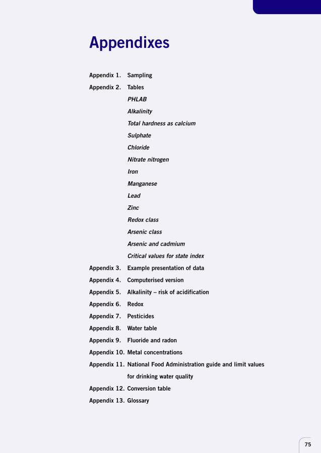
75

Appendix 1. Sampling

Appendix 2. Tables

PHLAB

Alkalinity

Total hardness as calcium

Sulphate

Chloride

Nitrate nitrogen

Iron

Manganese

Lead

Zinc

Redox class

Arsenic class

Arsenic and cadmium

Critical values for state index

Appendix 3. Example presentation of data

Appendix 4. Computerised version

Appendix 5. Alkalinity – risk of acidification

Appendix 6. Redox

Appendix 7. Pesticides

Appendix 8. Water table

Appendix 9. Fluoride and radon

Appendix 10. Metal concentrations

Appendix 11. National Food Administration guide and limit values

for drinking water quality

Appendix 12. Conversion table

Appendix 13. Glossary

Appendixes

77

How samples should be taken, what time of the year they should be taken

and how many should be taken. Further information is given in the Environ-

mental Monitoring Handbook, reached via the Swedish EPA home page:

www.environ.se (in Swedish only)

IntroductionModern analytical methods have made it possible to obtain increasinglyaccurate figures in areas of low concentrations. Knowledge of the entiresampling chain is needed to interpret these results: the sampling locationand its characteristics, sampling method, type of sampling vessel, treat-ment of samples, transport of samples, storage and analytical methods.If a proper comparison of findings is to be made, it is important to use thesame sampling procedure and treatment, or at least to ensure that the samefraction of the water is analysed.

Purpose of samplingThe purpose of sampling always determines where, how, and sometimesalso when, it is to be performed. Purposes include:• Examination of drinking water quality• Examination of raw water quality for drinking water production• Surveying groundwater quality in aquifers• Studies of changes in chemical composition of groundwater over time• Examination of pollutants in groundwater

Sampling for drinking water qualitySamples to examine the quality of water used for drinking purposes mustbe taken direct from the taps used for the purpose.

An analysis often gives an indication of the chemical composition ofthe groundwater, although the chemical composition of the water will havechanged to a varying extent on its way from the aquifer to the tap throughpipes and pressure tanks. Any filters, aeration devices or chemical additiveswill also change the chemical composition of the original groundwater.

If analyses of water taken from household taps are used for purposesother than checking drinking water quality, it is essential to make clear thefactors that may have affected the quality of the original groundwater.

Sampling

APPENDIX 1

78

Sampling to ascertain groundwater qualityGroundwater is seldom readily accessible at ground level. It usually has tobe brought to the surface in some way. Excavated and bored wells can beused to sample soil water and water in the bedrock. The most clearly defi-ned samples are obtained using tubes inserted into the ground.

Well samplesWell water is a mixture of groundwater seeping into the well at variouslevels. Sampling in wells therefore provides an integrated picture of thegroundwater present.

Wells bored in rockWater samples from borehole wells should be taken at as early a stage aspossible in the water distribution system, preferably before the pressuretank. To get a fresh groundwater sample, old water that has been standingin the well and the distribution system should be turned over by flushingthis water away before sampling.

Excavated wellsThe volume present is first replaced. It is best to take the sample straightfrom the well. This can be done using a container or pump made of inertmaterial. Otherwise, the procedure is the same as for wells bored in rock.

Samples from groundwater sampling tubesMore detailed surveys of the chemical composition of groundwater willrequire use of a sampling tube designed for the purpose. By inserting thetube filter down to the required level, it is possible to take samples from awell-defined part of the aquifer.

The water present in the sampling tube is replaced before sampling. Ifinterest is focused on the chemical composition of the layer in whichgroundwater flows, eg, fluvio-glacial deposits, the water volume can bereplaced several times over before samples are taken. If, however, the pri-mary concern is to monitor changes in groundwater chemistry over time ata given point, the volume present should not be replaced more than oneand a half times, so that the water in the immediate vicinity of the slit isforced into the tube.

The material of which the sampling tubes are made should be chosento take account of the chemical variables to be analysed. In particular, thechoice of materials is limited by the chemical substances naturally occur-ring in very low concentrations in the groundwater, such as heavy metalsand organic pollutants. Inert, colourless acrylic or polythene plastics arepreferable for heavy metals, whereas stainless metal tubes are best forsampling organic pollutants.

APPENDIX 1

79

Sampling of springsSamples of this kind need not come into contact with any foreign materialswhich could contaminate them, which is a good thing. The water flowscontinually and need not be replaced prior to sampling. Spring water ismixed and provides an integrated picture of the quality of the groundwaterpresent. Chemical composition may vary considerably during the year.

Sampling equipmentSampling equipment must always be made of inert materials, which is parti-cularly important if samples are to be analysed for heavy metals. Samplingequipment must be stored so that it is not contaminated (internally or exter-nally) between sampling occasions.

It must be possible to flush out tubes with metal-free deionised waterbetween sampling occasions. After each batch of samples has been taken thetubes should be placed in a bath of weak acid before being flushed out withmetal-free deionised water, in order to allow any metals adsorbed to theplastic to leach out.

Simple sampling equipment can easily be used to take samples fromnear-surface groundwater (6 - 9 m deep). By evacuating the air from a col-lection vessel using a normal suction pump, it is possible to create sufficientpressure to extract groundwater from a depth of around 7 m. This techniqueis often used nowadays. However, it is now possible to buy peristaltic pumpsand systems allowing on-line filtration (see below) and field analysis in flowcells in a closed system. This has the advantage that sample water does notcome into contact with air, thus preventing oxidation of some chemicalelements and changes the chemical composition of the water.

Some kind of container or submersible pump must be used wheregroundwater is too deep to be removed by suction. The essential thing is toensure that the pump does not contaminate the samples. Several “environ-mental sampling” pumps are now available on the market.

Wells bored in rock already have pumps fitted, as do most excavatedwells. However, in the latter case, the water should ideally be sampledstraight from the well using a sampling device made of inert materials.

FiltrationWater pumped up from a pipe contains a greater or lesser quantity of mine-ral particles. It is therefore necessary to filter samples before preservingthem using acid.

Dissolved metals are usually defined as the fraction passing through amembrane with a pore diameter of 0.40–0.45 µm. Colloids, hydroxides andsmall clay particles can also pass through, however. It is therefore better toterm the analysed fraction “filtrable” instead of “dissolved”. Filtration equip-ment should be made of teflon, polythene, polypropylene, plexiglass or poly-

APPENDIX 1

80

carbonate, which will withstand cleaning by leaching in an acid bath.Filtration using plastic syringes is one practical way of taking groundwa-

ter samples, firstly because the filtrate goes straight into the specimen bottleand secondly because the equipment is light and takes up little room. Filt-ration of anaerobic water should take place in an anaerobic environment ina closed system (see above). Otherwise, there is a risk of filters cloggingwhen iron is oxidised, which would also cause the retention of heavy metalsas flocculants with the iron hydroxide.

Filters should be cleaned using 0.05M HNO3 and be rinsed in the clea-nest possible deionised or distilled water.

SamplingReplacement of waterSampling always commences with replacement of the water to be sampled(see above). This also applies when examining drinking water quality. Inthat case, the water is allowed to flow evenly out of the cold water tap untilit reaches an even temperature.

Every time new samples are taken and collected in a vessel the vesselshould first be properly rinsed with the water to be sampled before it istransferred into different specimen bottles.

Sampling of water for analysis of anions, nutrients, conductivity and pesti-cides (see Tables 1 and 2)Water analysed for anions, nutrients, alkalinity and conductivity can becollected in the same bottle (a 250 ml polythene bottle with an airtightcap). Smaller quantities can be taken when sampling for individual parame-ters. It is important to fill the bottle to the top and to ensure that no airbubbles are trapped under the cap. Samples should be kept in cool, darkconditions during transport to the laboratory. Alkalinity, the various nu-trients and conductivity are analysed or measured within 24 hours. The listin Appendix 7, page 127 should be followed when sampling for pesticides.Different laboratories will need to use different combinations of analysispackages to cover the list. Information on requirements for vessels, volumesetc will be supplied by the laboratory used. This must have GLP status orbe accredited and must take part in annual test comparisons.

Sampling of water for analysis of metals (see Tables 1 and 2)Samples to be analysed for metals must be filtered before being preserved.Plastic gloves should be worn when samples are taken. The filtration proce-dure is as follows.

Rinse the filtration syringe with water from the collection vessel. Refillthe syringe. If a loose membrane filter is used, this should be secured in thefilter holder by plastic clips and be rinsed in situ with distilled or deionised

APPENDIX 1

81

APPENDIX 1

TABLE 1.

The seven aspects are assessed using the following parameters.

Parameter Name of, Sampling Required Preservation, Analytical methodvariable vessel volume treatment of samples(variable code)

Alkalinity Alkalinity, Polythene 100 ml Samples kept in cool, ALK_NP54DA1

(Alk) dark conditions. SS 028139 mod

Analysis within 24 hours or ALK_NTG DA

Arsenic Polythene See Filtration by membrane AS_DG DA

bottles footnote 2 filter (0.45 µm), preserva- AS_DSA DA

tion using 0.5 ml conc. HNO3

ICP-MS in

per 100 ml sample. After accordance with

this kept in cold store (+ 4°C) instrument manuals2

Pesticides

The list in Appendix 7, page 127 should be followed when sampling for pesticides. Different laboratories

will need to use different combinations of analysis packages to cover the list. Information on requirements

for vessels, volumes etc will supplied by the laboratory used. This must have GLP status or be accredited

and must take part in annual test comparisons.

metal-free water. If disposable filter holders are used, these should be adjus-ted when fitted on the syringe. The first 10 ml of water passing through thefilter should be discarded. The same applies if filtration is performed on-line.

Polythene bottles, cleaned in acid, to be used for metal analysis samples,are stored in double plastic bags. The remainder of the water in the syringe isfiltered down into the bottle. When the filter is changed, the filter holder isrinsed thoroughly several times over using metal-free water. The first 10 mlof water passing through the new filter are also discarded.

Samples for metal analyses are preserved using a 0.5 ml conc. HNO3

super-pure quality per 100 ml of sample. This should be done as soon aspossible under the cleanest possible conditions. If samples are preserved at alaboratory, this should be done in a sterile room. The outer plastic bag isremoved outside the clean room. Acid is added using a pipette with polypro-pylene tips, washed in acid solution.

Determination in the field and storage of samplesConductivity is determined in the field when water samples are taken, so asto minimise changes. These are best performed using a flow cell, which pre-vents contact between the sample and the atmosphere. Sample bottles arekept in a dark cold store (+4°C) until analysis begins.

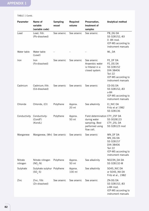
82

TABLE 1 Contd.

Parameter Name of Sampling Required Preservation, Analytical methodvariable vessel volume treatment of(variable code) samples

Lead Lead, filtr. See arsenic See arsenic See arsenic PB_DG DA(Pb-dissolved) SS 028152,-83

0 -84 mod.ICP-MS according toinstrument manuals

Water table Water table – – – WL_DA(Level)

Iron Iron See arsenic See arsenic See arsenic FE_DF DA(Fe-dissolved) Anaerobic water FE_DG DA

is filtered in a SS 028152closed system. DIN 38406

Teil 22ICP-MS according toinstrument manuals

Cadmium Cadmium, filtr. See arsenic See arsenic See arsenic CD-DG DA(Cd-dissolved) SS 028152,-83

o-84ICP-MS according toinstrument manuals

Chloride Chloride, (Cl) Polythene Approx. See alkalinity Cl_NIC DA20 ml Fritz et al 1982

SS 028136

Conductivity Conductivity- Polythene Approx. Field determination CTY_25F DA(CondF) 50 ml during water SS 0028123(KondL) sampling. Best CTY_25L DA

performed using SS 028123 modflow cell.

Manganese Manganese, (Mn) See arsenic See arsenic See arsenic MN_DF DAMN_DG DASS 028157DIN 38406Teil 22ICP-MS according toinstrument manuals

Nitrate Nitrate nitrogen Polythene Approx. See alkalinity NO23N_DA DAnitrogen (NO

3-N) 50 ml SS 028132-M

Sulphate Sulphate sulphur Polythene Approx. See alkalinity SO4S_NIC DA(SO

4-S) 100 ml or SO4S_NA DA

Fritz et al., 1982

Zinc Zinc, filtr. See arsenic See arsenic See arsenic ZN-DG DA(Zn-dissolved) SS 028152,-83

o-84 mod.ICP-MS according toinstrument manuals

APPENDIX 1

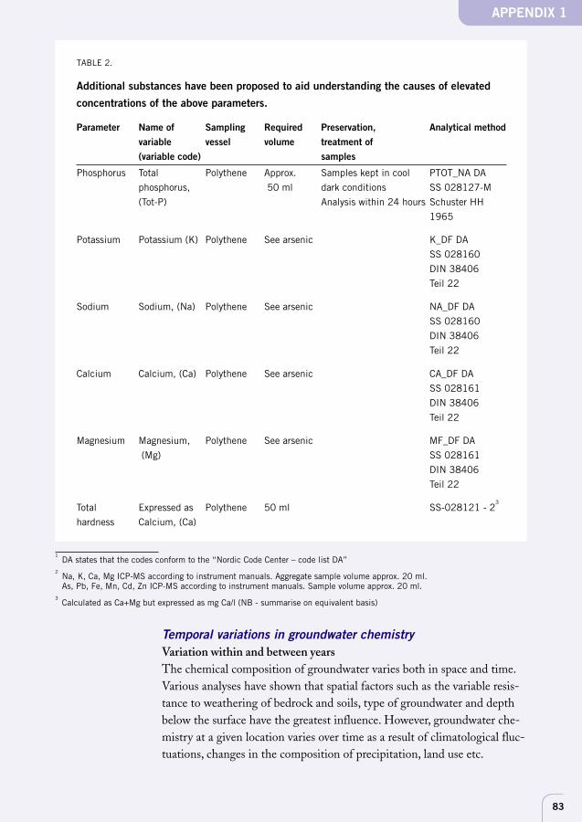
83

TABLE 2.

Additional substances have been proposed to aid understanding the causes of elevated

concentrations of the above parameters.

Parameter Name of Sampling Required Preservation, Analytical methodvariable vessel volume treatment of(variable code) samples

Phosphorus Total Polythene Approx. Samples kept in cool PTOT_NA DA

phosphorus, 50 ml dark conditions SS 028127-M

(Tot-P) Analysis within 24 hours Schuster HH

1965

Potassium Potassium (K) Polythene See arsenic K_DF DA

SS 028160

DIN 38406

Teil 22

Sodium Sodium, (Na) Polythene See arsenic NA_DF DA

SS 028160

DIN 38406

Teil 22

Calcium Calcium, (Ca) Polythene See arsenic CA_DF DA

SS 028161

DIN 38406

Teil 22

Magnesium Magnesium, Polythene See arsenic MF_DF DA

(Mg) SS 028161

DIN 38406

Teil 22

Total Expressed as Polythene 50 ml SS-028121 - 23

hardness Calcium, (Ca)

1DA states that the codes conform to the “Nordic Code Center – code list DA”

2Na, K, Ca, Mg ICP-MS according to instrument manuals. Aggregate sample volume approx. 20 ml.As, Pb, Fe, Mn, Cd, Zn ICP-MS according to instrument manuals. Sample volume approx. 20 ml.

3Calculated as Ca+Mg but expressed as mg Ca/l (NB - summarise on equivalent basis)

APPENDIX 1

Temporal variations in groundwater chemistryVariation within and between yearsThe chemical composition of groundwater varies both in space and time.Various analyses have shown that spatial factors such as the variable resis-tance to weathering of bedrock and soils, type of groundwater and depthbelow the surface have the greatest influence. However, groundwater che-mistry at a given location varies over time as a result of climatological fluc-tuations, changes in the composition of precipitation, land use etc.

84

Temporal variations can be split into variations over several years and thoseoccurring during a single year. One type of variation over a period of severalyears is referred to as trends. Analyses of variations in groundwater chemis-try over time from the early 1980s to the mid-1990s show that statisticallysignificant trends do sometimes occur. For example, sulphate concentrationsfell in the 1980s following a decrease in sulphur deposition. This trend isfairly widespread across the country. There are also more statistically scatte-red trends for other parameters.

In total, chemical constituents in groundwater at a given monitoringlocation typically show variability, as expressed in terms of variation coeffi-cients (mean/standard deviation), ranging from 5–30 per cent, althoughhigher variation coefficients do occur, particularly in water with a low ioncontent. (In comparison, typical variation coefficients for water from diffe-rent type areas are in the order of 50–100 per cent, lower in areas of sedi-mentary bedrock and higher in coarse soils derived from igneous and meta-morphic rock). For alkalinity, hardness and pH, for example, the variationcoefficient usually falls with rising concentrations, which often occurs inrelation to increasing age of groundwater, increasing depth below the surfa-ce, falling resistance to weathering of rock and soil and the presence of con-fined aquifers under clays and other impermeable soils. Variations in theconcentrations of other constituents, such as sulphate, are less, or not at all,dependent on depth.

Examples of climatological factors influencing the chemical compositionof groundwater are:• snow melt or heavy, persistent precipitation, resulting in low-ion near-

surface groundwater, particularly in coarse soils resistant to weathering• a drop in the water table following a long drought, which may cause

oxidation of sulphides, leading to rising sulphate concentrations andfalling pH

• a rising water table after a dry period, which may cause iron and manga-nese compounds precipitated in the surface layer to dissolve in thegroundwater

Variation in concentrations within groundwater environmentsUsing its groundwater chemistry database, the Swedish Geological Surveyhas studied how the 90 per cent confidence interval for conductivity varieswith sample size. (This means that there is a 90 per cent likelihood that thetrue mean lies within the limits of the confidence interval.) Conductivitywas chosen because it represents the total concentration of dissolved sub-stances in the groundwater. Figure 1 shows that the 90 per cent confidenceinterval is approximately 1 to 2 times the mean when 10 samples are taken,but is only one third as great when 90 samples are taken. As may be seenfrom the graph, the variation in concentration is greatest in groundwater

APPENDIX 1

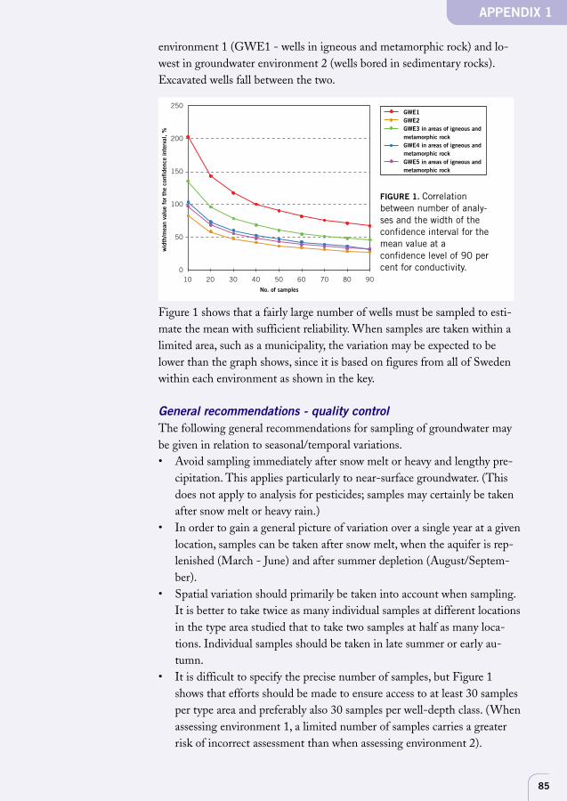
85

environment 1 (GWE1 - wells in igneous and metamorphic rock) and lo-west in groundwater environment 2 (wells bored in sedimentary rocks).Excavated wells fall between the two.

Figure 1 shows that a fairly large number of wells must be sampled to esti-mate the mean with sufficient reliability. When samples are taken within alimited area, such as a municipality, the variation may be expected to belower than the graph shows, since it is based on figures from all of Swedenwithin each environment as shown in the key.

General recommendations - quality controlThe following general recommendations for sampling of groundwater maybe given in relation to seasonal/temporal variations.• Avoid sampling immediately after snow melt or heavy and lengthy pre-

cipitation. This applies particularly to near-surface groundwater. (Thisdoes not apply to analysis for pesticides; samples may certainly be takenafter snow melt or heavy rain.)

• In order to gain a general picture of variation over a single year at a givenlocation, samples can be taken after snow melt, when the aquifer is rep-lenished (March - June) and after summer depletion (August/Septem-ber).

• Spatial variation should primarily be taken into account when sampling.It is better to take twice as many individual samples at different locationsin the type area studied that to take two samples at half as many loca-tions. Individual samples should be taken in late summer or early au-tumn.

• It is difficult to specify the precise number of samples, but Figure 1shows that efforts should be made to ensure access to at least 30 samplesper type area and preferably also 30 samples per well-depth class. (Whenassessing environment 1, a limited number of samples carries a greaterrisk of incorrect assessment than when assessing environment 2).

APPENDIX 1

10 20 30 40 50 60 70 80 90

antal prov

konf

iden

sint

erva

llets

bre

dd/m

edel

värd

e, %

250

200

150

100

50

0

gvm=1

gvm=2

gvm=3 i urbergsområden



FIGURE 1. Correlationbetween number of analy-ses and the width of theconfidence interval for themean value at aconfidence level of 90 percent for conductivity.

GWE1GWE2GWE3 in areas of igneous andmetamorphic rockGWE4 in areas of igneous andmetamorphic rockGWE5 in areas of igneous andmetamorphic rock

No. of samples

wid

th/m

ean

valu

e fo

r th

e co

nfid

ence

inte

rval

, %

86

A reference database is presented here, compiled from nearly 30,000 wells.

Most of the analyses were collected in the 1980s. Concentration distribu-

tions for 35 type areas, each divided into two well-depth classes, are shown

in table form.

Explanation of the concentration distributions shown in Tables1–12A combination of two letters and one number is given in Tables 1–12 un-der the heading “Type area – Depth”. The first letter indicates the regionin which the area is located. The figure indicates the relevant groundwaterenvironment and the second letter stands for the well-depth class. (”Divi-sion into type areas” is presented in the chapter of the same name.)

For instance, G3d is the reference database for all deep wells (d) insurface aquifers in moraine and fluvial outwash (3) from the coast of Norr-land (northern Sweden) (G).

The distribution into shallow and deep wells:

Groundwater Explanationenvironment-depth1g Igneous bedrock, < 65 m

1d Igneous bedrock, > 65 m

2g Sedimentary bedrock, < 65 m

2d Sedimentary bedrock, > 65 m

3g Surface aquifers in moraine and fluvial outwash, < 4 m

3d Surface aquifers in moraine and fluvial outwash, > 4 m

4g Surface aquifers in fluvio-glacial deposits, < 4 m

4d Surface aquifers in fluvio-glacial deposits, > 4 m

5g Confined aquifers in moraine and fluvio-glacial deposits, < 4 m

5d Confined aquifers in moraine and fluvio-glacial deposits, > 4 m

Other codes used in Tables 1–12:

Code Explanation

N Number of analyses in the reference database

P5, P95 5th/95th percentile of the data

Q1, Q3 1st/3rd quartile, ie, 25/75 per cent of the data

Median The median figure, ie, the figure in the middle of the data

Table 13: “Critical values for weighting index” is presented in the chapterentitled “Instructions for deviation test”.

Tables

APPENDIX 2

87

APPENDIX 2

Parameters in the tablesRedoxThe deviation test is suitable for the constituents in Tables 1–10 in thisappendix.

The method cannot be used for the distribution of redox classes shownin Table 11, since that table differs from the others. The redox classes arethose presented in the chapter on “Redox”, Table 11 (although the fifthclass, for mixed water, is not included). If a high redox class occurs at lowpercentile or quartile values, this means that anaerobic water is common inthat environment. For example, it may be seen that at least 25 per cent ofwells monitored in environment type A2d (deep wells in sedimentaryrocks in region A - Skåne and elsewhere) belong to class 4 (anaerobicwater, where sulphate has been reduced and hydrogen sulphide may occur),and only 5–25 per cent of wells belong to class 1, with high redox potentialand low concentrations of iron and manganese. On the other hand, Table11 shows that at least 75 per cent of wells monitored in environment typeG3g (shallow wells in moraine or outwash in region G – coast of Norr-land, northern Sweden) belong to class 1 and that class 4 only occurs infewer than 5 per cent of wells.

Arsenic (As) and Cadmium (Cd)The tables for arsenic and cadmium are only divided into wells bored insoil or rock. The number of analyses is insufficient to allow a further distri-bution. Nor is there sufficient data to perform deviation tests.

PHLAB and total hardness (as calcium, Ca)The tables showing distributions of the values for PHLAB and concentra-tions for total hardness have been included even though they are not usedas parameters in the Groundwater report.

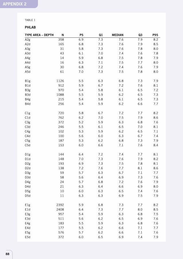
88

TABLE 1

PHLAB

TYPE AREA – DEPTH N P5 Q1 MEDIAN Q3 P95A2g 358 6.9 7.3 7.6 7.9 8.2

A2d 165 6.8 7.3 7.6 7.9 8.5

A3g 31 5.8 7.3 7.6 7.8 8.0

A3d 43 6.1 7.0 7.4 7.6 7.8

A4g 14 5.9 6.8 7.5 7.8 7.9

A4d 16 6.3 7.1 7.5 7.7 8.0

A5g 30 6.8 7.2 7.4 7.6 7.9

A5d 61 7.0 7.3 7.5 7.8 8.0

B1g 1126 5.5 6.3 6.8 7.3 7.9

B1d 912 5.9 6.7 7.2 7.6 8.1

B3g 970 5.4 5.8 6.1 6.5 7.2

B3d 1088 5.5 5.9 6.2 6.5 7.3

B4g 215 5.4 5.8 6.1 6.5 7.3

B4d 256 5.4 5.9 6.2 6.6 7.7

C1g 720 5.8 6.7 7.2 7.7 8.2

C1d 762 6.2 7.0 7.5 7.9 8.6

C3g 372 5.2 5.9 6.3 6.8 7.6

C3d 246 5.5 6.1 6.5 7.0 8.1

C4g 102 5.3 5.9 6.2 6.5 7.1

C4d 100 5.6 6.0 6.3 6.7 7.4

C5g 187 5.3 6.2 6.8 7.3 7.9

C5d 153 6.0 6.6 7.1 7.6 8.4

D1g 144 6.4 7.2 7.4 7.7 8.1

D1d 148 7.0 7.3 7.6 7.9 8.2

D2g 193 6.9 7.3 7.5 7.8 8.1

D2d 138 7.2 7.6 7.7 8.1 8.6

D3g 59 5.7 6.3 6.7 7.1 7.7

D3d 58 5.6 6.4 6.9 7.3 7.6

D4g 24 5.7 6.8 7.2 7.6 7.9

D4d 21 6.3 6.4 6.6 6.9 8.0

D5g 10 6.0 6.3 6.5 7.4 7.6

D5d 11 6.3 6.3 6.9 7.5 7.9

E1g 2392 5.9 6.8 7.3 7.7 8.2

E1d 2408 6.4 7.3 7.7 8.0 8.5

E3g 957 5.4 5.9 6.3 6.8 7.5

E3d 511 5.6 6.2 6.5 6.9 7.6

E4g 183 5.5 5.9 6.3 6.8 7.6

E4d 177 5.5 6.2 6.6 7.1 7.7

E5g 576 5.7 6.2 6.6 7.1 7.6

E5d 372 6.0 6.5 6.9 7.4 7.9

APPENDIX 2

89

TABLE 1 Contd.

TYPE AREA – DEPTH N P5 Q1 MEDIAN Q3 P95F1g 851 6.7 7.2 7.5 7.9 8.4

F1d 994 6.9 7.4 7.8 8.1 8.5

F3g 38 6.0 6.6 7.0 7.2 7.7

F3d 40 6.0 6.8 7.1 7.4 8.0

F4g 5 6.3 6.9 7.3 7.4 7.8

F4d 18 6.3 6.8 7.4 7.6 7.8

F5g 28 6.0 6.9 7.1 7.5 7.7

F5d 20 6.6 7.0 7.3 7.4 7.9

G1g 869 6.2 6.9 7.5 7.9 8.4

G1d 772 6.7 7.5 7.9 8.2 8.7

G3g 786 5.5 6.0 6.3 6.6 7.2

G3d 414 5.8 6.2 6.4 6.8 7.4

G4g 83 5.8 6.1 6.4 6.9 7.5

G4d 91 5.7 6.3 6.7 7.2 8.2

G5g 261 5.7 6.2 6.5 6.8 7.5

G5d 95 5.9 6.2 6.5 6.9 7.5

H1g 60 6.4 7.3 7.7 8.0 8.4

H1d 19 6.6 7.5 7.7 8.2 9.0

H2g 53 6.9 7.3 7.8 8.0 8.3

H2d 30 7.1 7.6 8.0 8.3 9.3

H3g 74 5.9 6.3 6.9 7.2 7.5

H3d 35 6.1 6.5 6.8 7.3 7.5

H4g 14 6.0 6.1 6.4 7.2 7.8

H4d 9 5.9 6.4 7.0 7.2 7.7

H5g 26 6.4 6.7 7.1 7.3 7.3

H5d 27 6.2 6.6 7.1 7.3 7.6

I1g 672 5.9 6.7 7.2 7.7 8.2

I1d 340 6.1 7.0 7.5 7.9 8.3

I3g 631 5.5 5.9 6.2 6.6 7.3

I3d 285 5.6 6.1 6.4 6.7 7.4

I4g 79 5.6 6.0 6.3 6.7 7.6

I4d 59 5.9 6.1 6.5 6.9 7.9

APPENDIX 2

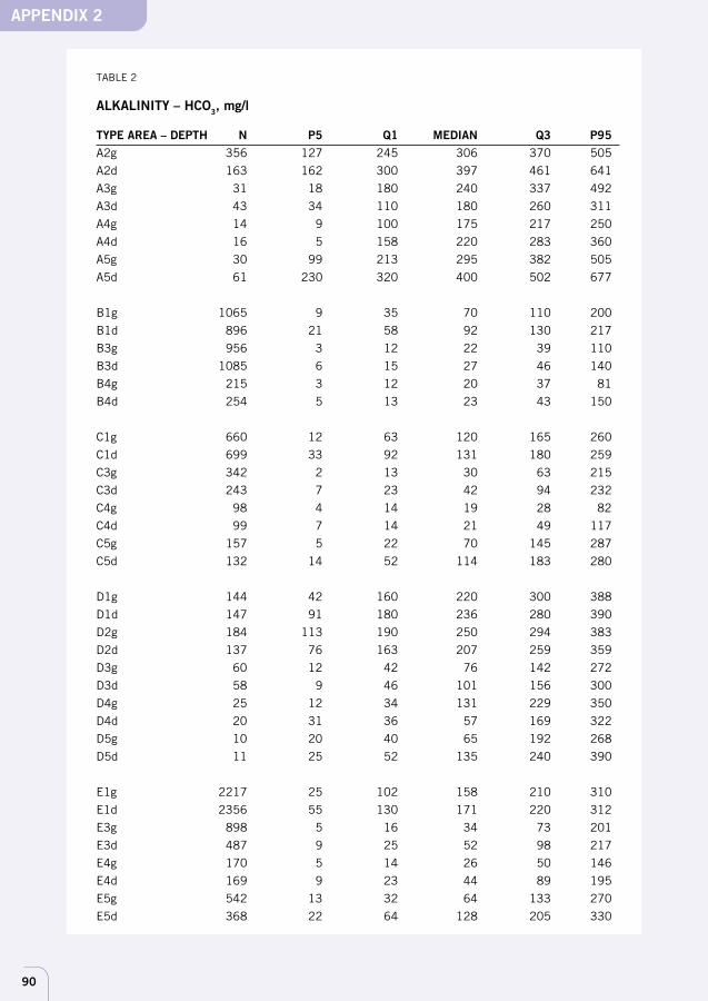
90

TABLE 2

ALKALINITY – HCO3, mg/l

TYPE AREA – DEPTH N P5 Q1 MEDIAN Q3 P95A2g 356 127 245 306 370 505

A2d 163 162 300 397 461 641

A3g 31 18 180 240 337 492

A3d 43 34 110 180 260 311

A4g 14 9 100 175 217 250

A4d 16 5 158 220 283 360

A5g 30 99 213 295 382 505

A5d 61 230 320 400 502 677

B1g 1065 9 35 70 110 200

B1d 896 21 58 92 130 217

B3g 956 3 12 22 39 110

B3d 1085 6 15 27 46 140

B4g 215 3 12 20 37 81

B4d 254 5 13 23 43 150

C1g 660 12 63 120 165 260

C1d 699 33 92 131 180 259

C3g 342 2 13 30 63 215

C3d 243 7 23 42 94 232

C4g 98 4 14 19 28 82

C4d 99 7 14 21 49 117

C5g 157 5 22 70 145 287

C5d 132 14 52 114 183 280

D1g 144 42 160 220 300 388

D1d 147 91 180 236 280 390

D2g 184 113 190 250 294 383

D2d 137 76 163 207 259 359

D3g 60 12 42 76 142 272

D3d 58 9 46 101 156 300

D4g 25 12 34 131 229 350

D4d 20 31 36 57 169 322

D5g 10 20 40 65 192 268

D5d 11 25 52 135 240 390

E1g 2217 25 102 158 210 310

E1d 2356 55 130 171 220 312

E3g 898 5 16 34 73 201

E3d 487 9 25 52 98 217

E4g 170 5 14 26 50 146

E4d 169 9 23 44 89 195

E5g 542 13 32 64 133 270

E5d 368 22 64 128 205 330

APPENDIX 2

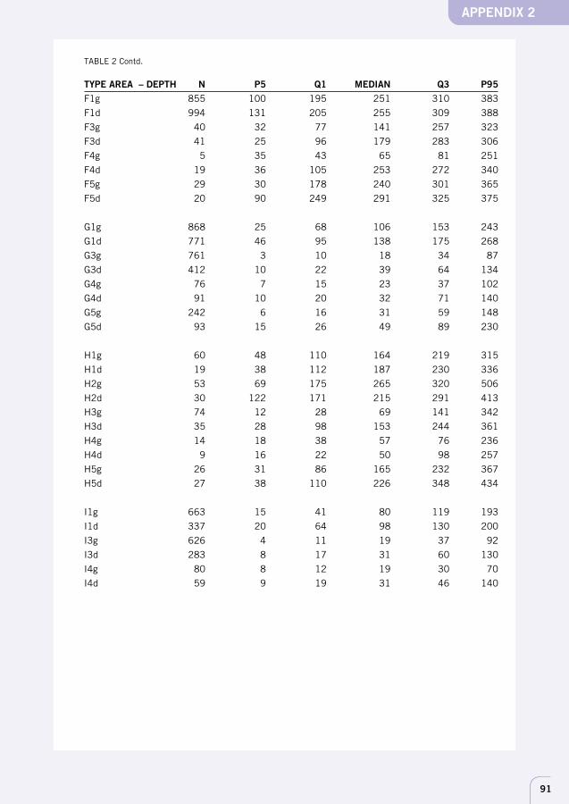
91

TABLE 2 Contd.

TYPE AREA – DEPTH N P5 Q1 MEDIAN Q3 P95F1g 855 100 195 251 310 383

F1d 994 131 205 255 309 388

F3g 40 32 77 141 257 323

F3d 41 25 96 179 283 306

F4g 5 35 43 65 81 251

F4d 19 36 105 253 272 340

F5g 29 30 178 240 301 365

F5d 20 90 249 291 325 375

G1g 868 25 68 106 153 243

G1d 771 46 95 138 175 268

G3g 761 3 10 18 34 87

G3d 412 10 22 39 64 134

G4g 76 7 15 23 37 102

G4d 91 10 20 32 71 140

G5g 242 6 16 31 59 148

G5d 93 15 26 49 89 230

H1g 60 48 110 164 219 315

H1d 19 38 112 187 230 336

H2g 53 69 175 265 320 506

H2d 30 122 171 215 291 413

H3g 74 12 28 69 141 342

H3d 35 28 98 153 244 361

H4g 14 18 38 57 76 236

H4d 9 16 22 50 98 257

H5g 26 31 86 165 232 367

H5d 27 38 110 226 348 434

I1g 663 15 41 80 119 193

I1d 337 20 64 98 130 200

I3g 626 4 11 19 37 92

I3d 283 8 17 31 60 130

I4g 80 8 12 19 30 70

I4d 59 9 19 31 46 140

APPENDIX 2

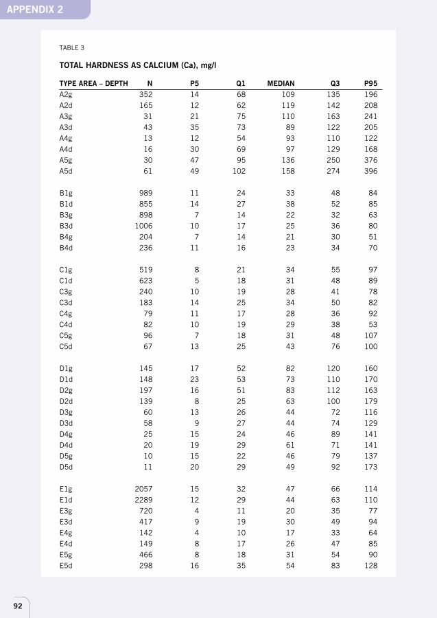
92

TABLE 3

TOTAL HARDNESS AS CALCIUM (Ca), mg/l


A2d 165 12 62 119 142 208

A3g 31 21 75 110 163 241

A3d 43 35 73 89 122 205

A4g 13 12 54 93 110 122

A4d 16 30 69 97 129 168

A5g 30 47 95 136 250 376

A5d 61 49 102 158 274 396

B1g 989 11 24 33 48 84

B1d 855 14 27 38 52 85

B3g 898 7 14 22 32 63

B3d 1006 10 17 25 36 80

B4g 204 7 14 21 30 51

B4d 236 11 16 23 34 70

C1g 519 8 21 34 55 97

C1d 623 5 18 31 48 89

C3g 240 10 19 28 41 78

C3d 183 14 25 34 50 82

C4g 79 11 17 28 36 92

C4d 82 10 19 29 38 53

C5g 96 7 18 31 48 107

C5d 67 13 25 43 76 100

D1g 145 17 52 82 120 160

D1d 148 23 53 73 110 170

D2g 197 16 51 83 112 163

D2d 139 8 25 63 100 179

D3g 60 13 26 44 72 116

D3d 58 9 27 44 74 129

D4g 25 15 24 46 89 141

D4d 20 19 29 61 71 141

D5g 10 15 22 46 79 137

D5d 11 20 29 49 92 173

E1g 2057 15 32 47 66 114

E1d 2289 12 29 44 63 110

E3g 720 4 11 20 35 77

E3d 417 9 19 30 49 94

E4g 142 4 10 17 33 64

E4d 149 8 17 26 47 85

E5g 466 8 18 31 54 90

E5d 298 16 35 54 83 128

APPENDIX 2

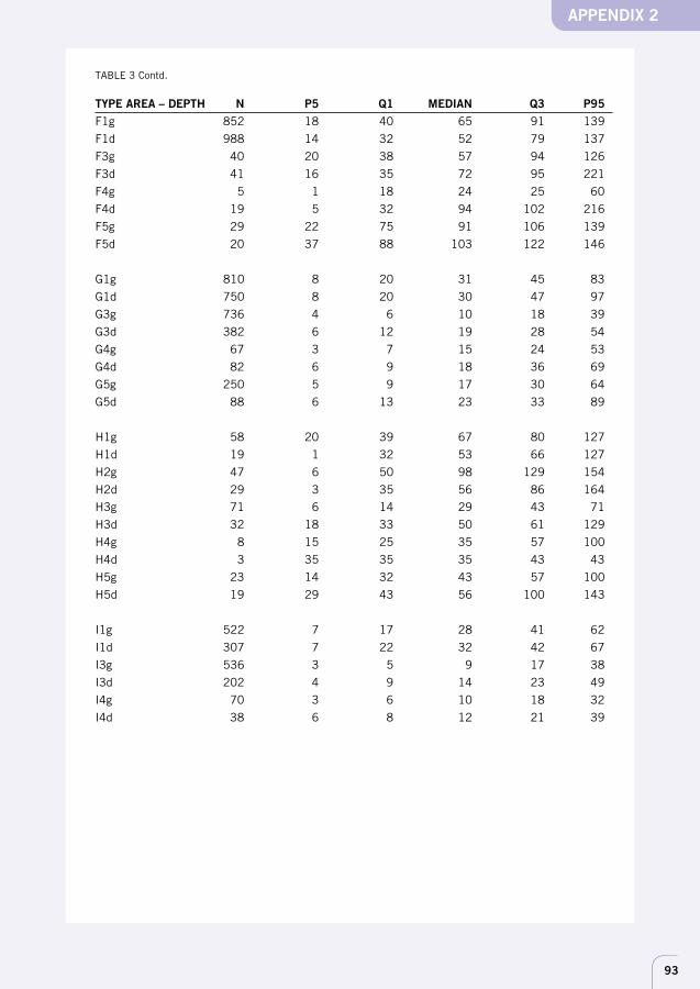
93

TABLE 3 Contd.


F1d 988 14 32 52 79 137

F3g 40 20 38 57 94 126

F3d 41 16 35 72 95 221

F4g 5 1 18 24 25 60

F4d 19 5 32 94 102 216

F5g 29 22 75 91 106 139

F5d 20 37 88 103 122 146

G1g 810 8 20 31 45 83

G1d 750 8 20 30 47 97

G3g 736 4 6 10 18 39

G3d 382 6 12 19 28 54

G4g 67 3 7 15 24 53

G4d 82 6 9 18 36 69

G5g 250 5 9 17 30 64

G5d 88 6 13 23 33 89

H1g 58 20 39 67 80 127

H1d 19 1 32 53 66 127

H2g 47 6 50 98 129 154

H2d 29 3 35 56 86 164

H3g 71 6 14 29 43 71

H3d 32 18 33 50 61 129

H4g 8 15 25 35 57 100

H4d 3 35 35 35 43 43

H5g 23 14 32 43 57 100

H5d 19 29 43 56 100 143

I1g 522 7 17 28 41 62

I1d 307 7 22 32 42 67

I3g 536 3 5 9 17 38

I3d 202 4 9 14 23 49

I4g 70 3 6 10 18 32

I4d 38 6 8 12 21 39

APPENDIX 2

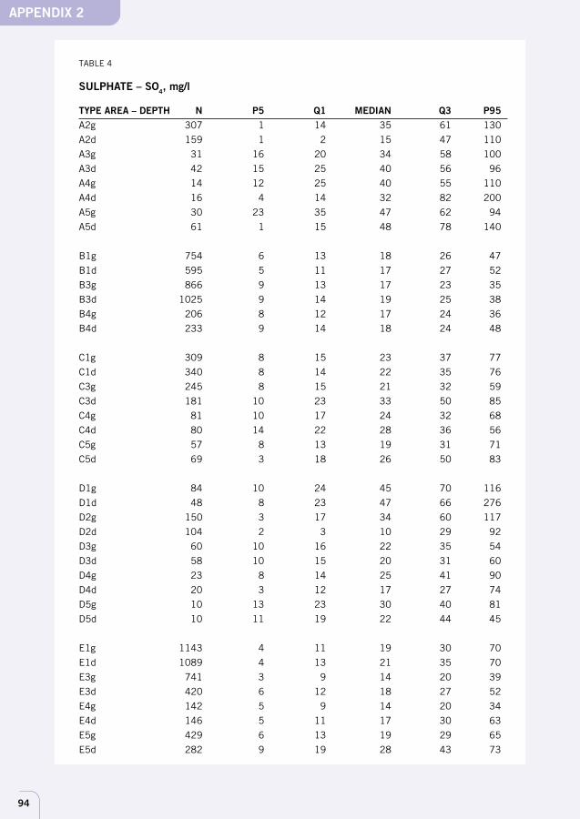
94

TABLE 4

SULPHATE – SO4, mg/l


A2d 159 1 2 15 47 110

A3g 31 16 20 34 58 100

A3d 42 15 25 40 56 96

A4g 14 12 25 40 55 110

A4d 16 4 14 32 82 200

A5g 30 23 35 47 62 94

A5d 61 1 15 48 78 140

B1g 754 6 13 18 26 47

B1d 595 5 11 17 27 52

B3g 866 9 13 17 23 35

B3d 1025 9 14 19 25 38

B4g 206 8 12 17 24 36

B4d 233 9 14 18 24 48

C1g 309 8 15 23 37 77

C1d 340 8 14 22 35 76

C3g 245 8 15 21 32 59

C3d 181 10 23 33 50 85

C4g 81 10 17 24 32 68

C4d 80 14 22 28 36 56

C5g 57 8 13 19 31 71

C5d 69 3 18 26 50 83

D1g 84 10 24 45 70 116

D1d 48 8 23 47 66 276

D2g 150 3 17 34 60 117

D2d 104 2 3 10 29 92

D3g 60 10 16 22 35 54

D3d 58 10 15 20 31 60

D4g 23 8 14 25 41 90

D4d 20 3 12 17 27 74

D5g 10 13 23 30 40 81

D5d 10 11 19 22 44 45

E1g 1143 4 11 19 30 70

E1d 1089 4 13 21 35 70

E3g 741 3 9 14 20 39

E3d 420 6 12 18 27 52

E4g 142 5 9 14 20 34

E4d 146 5 11 17 30 63

E5g 429 6 13 19 29 65

E5d 282 9 19 28 43 73

APPENDIX 2

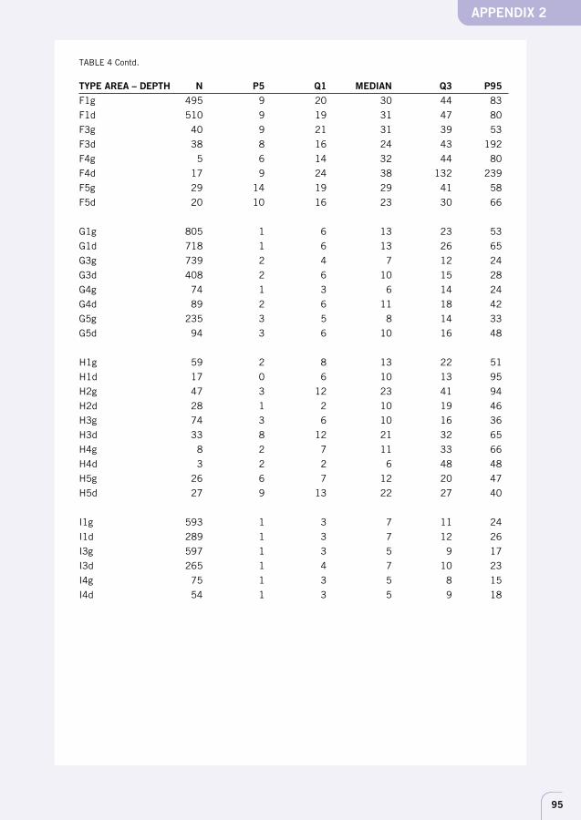
95

TABLE 4 Contd.


F1d 510 9 19 31 47 80

F3g 40 9 21 31 39 53

F3d 38 8 16 24 43 192

F4g 5 6 14 32 44 80

F4d 17 9 24 38 132 239

F5g 29 14 19 29 41 58

F5d 20 10 16 23 30 66

G1g 805 1 6 13 23 53

G1d 718 1 6 13 26 65

G3g 739 2 4 7 12 24

G3d 408 2 6 10 15 28

G4g 74 1 3 6 14 24

G4d 89 2 6 11 18 42

G5g 235 3 5 8 14 33

G5d 94 3 6 10 16 48

H1g 59 2 8 13 22 51

H1d 17 0 6 10 13 95

H2g 47 3 12 23 41 94

H2d 28 1 2 10 19 46

H3g 74 3 6 10 16 36

H3d 33 8 12 21 32 65

H4g 8 2 7 11 33 66

H4d 3 2 2 6 48 48

H5g 26 6 7 12 20 47

H5d 27 9 13 22 27 40

I1g 593 1 3 7 11 24

I1d 289 1 3 7 12 26

I3g 597 1 3 5 9 17

I3d 265 1 4 7 10 23

I4g 75 1 3 5 8 15

I4d 54 1 3 5 9 18

APPENDIX 2

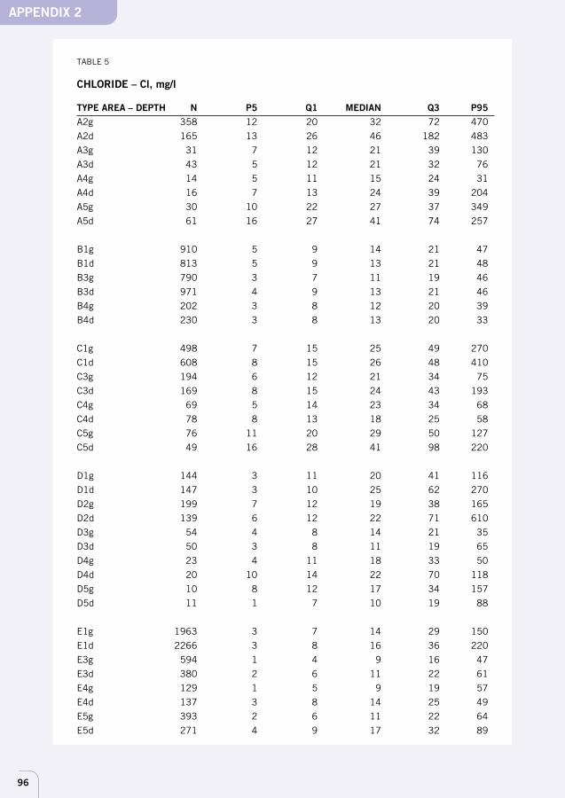
96

TABLE 5

CHLORIDE – Cl, mg/l


A2d 165 13 26 46 182 483

A3g 31 7 12 21 39 130

A3d 43 5 12 21 32 76

A4g 14 5 11 15 24 31

A4d 16 7 13 24 39 204

A5g 30 10 22 27 37 349

A5d 61 16 27 41 74 257

B1g 910 5 9 14 21 47

B1d 813 5 9 13 21 48

B3g 790 3 7 11 19 46

B3d 971 4 9 13 21 46

B4g 202 3 8 12 20 39

B4d 230 3 8 13 20 33

C1g 498 7 15 25 49 270

C1d 608 8 15 26 48 410

C3g 194 6 12 21 34 75

C3d 169 8 15 24 43 193

C4g 69 5 14 23 34 68

C4d 78 8 13 18 25 58

C5g 76 11 20 29 50 127

C5d 49 16 28 41 98 220

D1g 144 3 11 20 41 116

D1d 147 3 10 25 62 270

D2g 199 7 12 19 38 165

D2d 139 6 12 22 71 610

D3g 54 4 8 14 21 35

D3d 50 3 8 11 19 65

D4g 23 4 11 18 33 50

D4d 20 10 14 22 70 118

D5g 10 8 12 17 34 157

D5d 11 1 7 10 19 88

E1g 1963 3 7 14 29 150

E1d 2266 3 8 16 36 220

E3g 594 1 4 9 16 47

E3d 380 2 6 11 22 61

E4g 129 1 5 9 19 57

E4d 137 3 8 14 25 49

E5g 393 2 6 11 22 64

E5d 271 4 9 17 32 89

APPENDIX 2

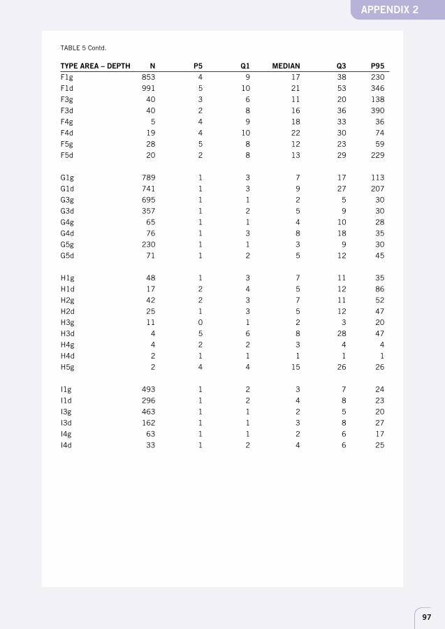
97

TABLE 5 Contd.


F1d 991 5 10 21 53 346

F3g 40 3 6 11 20 138

F3d 40 2 8 16 36 390

F4g 5 4 9 18 33 36

F4d 19 4 10 22 30 74

F5g 28 5 8 12 23 59

F5d 20 2 8 13 29 229

G1g 789 1 3 7 17 113

G1d 741 1 3 9 27 207

G3g 695 1 1 2 5 30

G3d 357 1 2 5 9 30

G4g 65 1 1 4 10 28

G4d 76 1 3 8 18 35

G5g 230 1 1 3 9 30

G5d 71 1 2 5 12 45

H1g 48 1 3 7 11 35

H1d 17 2 4 5 12 86

H2g 42 2 3 7 11 52

H2d 25 1 3 5 12 47

H3g 11 0 1 2 3 20

H3d 4 5 6 8 28 47

H4g 4 2 2 3 4 4

H4d 2 1 1 1 1 1

H5g 2 4 4 15 26 26

I1g 493 1 2 3 7 24

I1d 296 1 2 4 8 23

I3g 463 1 1 2 5 20

I3d 162 1 1 3 8 27

I4g 63 1 1 2 6 17

I4d 33 1 2 4 6 25

APPENDIX 2

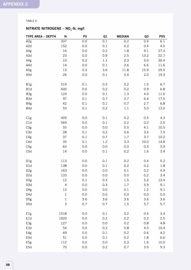
98

TABLE 6

NITRATE NITROGENE – NO3-N, mg/l


A2d 152 0.0 0.1 0.2 0.4 4.5

A3g 16 0.0 0.2 1.8 9.1 27.3

A3d 23 0.0 0.9 2.5 13.2 22.7

A4g 10 0.2 1.1 2.3 5.0 36.4

A4d 14 0.0 0.1 2.6 6.6 11.6

A5g 13 0.3 3.6 11.8 15.9 29.5

A5d 26 0.0 0.1 0.4 2.0 19.3

B1g 519 0.1 0.2 0.2 1.5 6.7

B1d 600 0.0 0.2 0.2 0.9 6.8

B3g 124 0.0 0.1 1.3 4.0 11.6

B3d 97 0.1 0.7 2.7 6.4 17.5

B4g 42 0.1 0.1 0.7 2.7 6.8

B4d 53 0.1 0.2 1.1 5.0 13.0

C1g 405 0.0 0.1 0.2 0.5 4.3

C1d 569 0.0 0.1 0.2 0.2 2.0

C3g 55 0.0 0.0 0.5 4.1 10.5

C3d 28 0.1 0.2 0.6 3.4 7.0

C4g 37 0.1 0.7 1.7 3.7 10.2

C4d 35 0.1 1.2 3.3 10.0 14.8

C5g 63 0.0 0.0 0.0 0.5 3.9

C5d 14 0.0 0.1 0.2 1.6 3.4

D1g 113 0.0 0.1 0.2 0.4 5.2

D1d 138 0.0 0.1 0.2 0.2 1.8

D2g 163 0.0 0.0 0.1 0.2 4.9

D2d 133 0.0 0.0 0.0 0.2 3.4

D3g 12 0.1 0.3 1.5 5.2 13.4

D3d 4 0.0 0.3 1.7 5.9 9.1

D4g 13 0.0 0.0 0.1 1.2 9.1

D4d 1 0.0 0.0 0.0 0.0 0.0

D5g 1 3.6 3.6 3.6 3.6 3.6

D5d 3 0.7 0.7 1.5 5.7 5.7

E1g 1518 0.0 0.1 0.2 0.4 3.4

E1d 1920 0.0 0.2 0.2 0.2 2.5

E3g 127 0.0 0.0 0.2 0.8 4.8

E3d 54 0.0 0.2 0.8 4.5 10.4

E4g 49 0.0 0.1 0.2 0.6 4.2

E4d 51 0.0 0.1 0.2 1.8 6.6

E5g 112 0.0 0.0 0.3 1.6 10.0

E5d 70 0.0 0.2 0.7 3.0 9.3

-

APPENDIX 2

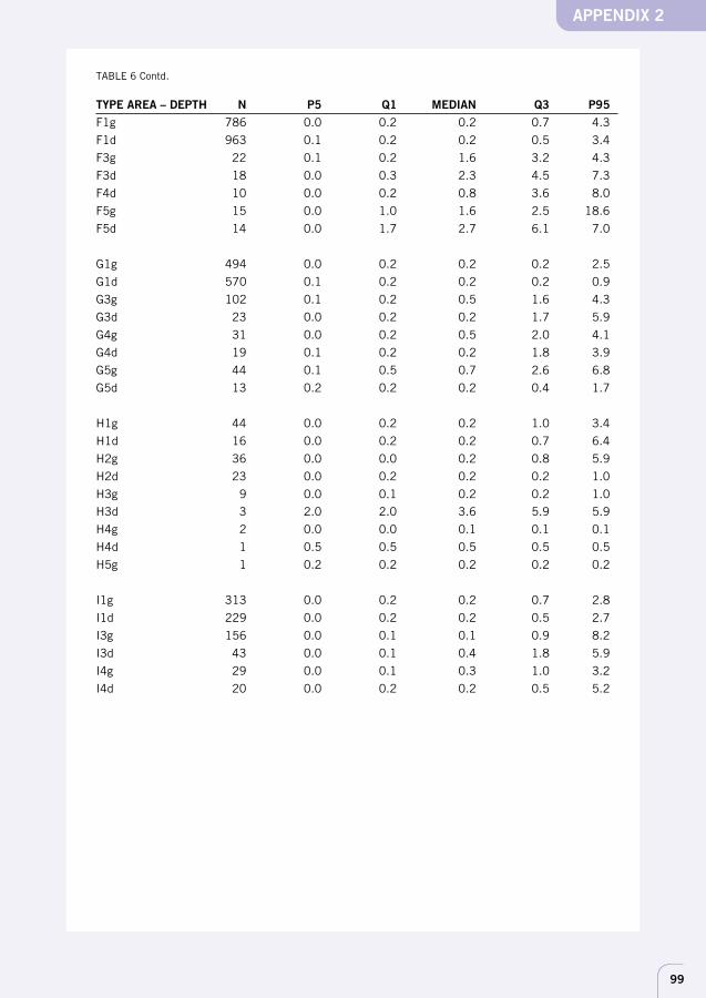
99

TABLE 6 Contd.


F1d 963 0.1 0.2 0.2 0.5 3.4

F3g 22 0.1 0.2 1.6 3.2 4.3

F3d 18 0.0 0.3 2.3 4.5 7.3

F4d 10 0.0 0.2 0.8 3.6 8.0

F5g 15 0.0 1.0 1.6 2.5 18.6

F5d 14 0.0 1.7 2.7 6.1 7.0

G1g 494 0.0 0.2 0.2 0.2 2.5

G1d 570 0.1 0.2 0.2 0.2 0.9

G3g 102 0.1 0.2 0.5 1.6 4.3

G3d 23 0.0 0.2 0.2 1.7 5.9

G4g 31 0.0 0.2 0.5 2.0 4.1

G4d 19 0.1 0.2 0.2 1.8 3.9

G5g 44 0.1 0.5 0.7 2.6 6.8

G5d 13 0.2 0.2 0.2 0.4 1.7

H1g 44 0.0 0.2 0.2 1.0 3.4

H1d 16 0.0 0.2 0.2 0.7 6.4

H2g 36 0.0 0.0 0.2 0.8 5.9

H2d 23 0.0 0.2 0.2 0.2 1.0

H3g 9 0.0 0.1 0.2 0.2 1.0

H3d 3 2.0 2.0 3.6 5.9 5.9

H4g 2 0.0 0.0 0.1 0.1 0.1

H4d 1 0.5 0.5 0.5 0.5 0.5

H5g 1 0.2 0.2 0.2 0.2 0.2

I1g 313 0.0 0.2 0.2 0.7 2.8

I1d 229 0.0 0.2 0.2 0.5 2.7

I3g 156 0.0 0.1 0.1 0.9 8.2

I3d 43 0.0 0.1 0.4 1.8 5.9

I4g 29 0.0 0.1 0.3 1.0 3.2

I4d 20 0.0 0.2 0.2 0.5 5.2

APPENDIX 2

100

TABLE 7

IRON – Fe,mg/l


A2d 153 0.02 0.12 0.78 2.10 11.00

A3g 23 0.03 0.03 0.05 0.25 1.01

A3d 30 0.03 0.03 0.03 0.36 3.40

A4g 14 0.01 0.03 0.03 0.04 0.63

A4d 16 0.03 0.06 0.37 1.69 6.00

A5g 13 0.03 0.03 0.03 0.03 0.58

A5d 26 0.03 0.03 0.23 3.50 7.00

B1g 767 0.03 0.05 0.15 0.67 4.70

B1d 717 0.03 0.05 0.16 0.43 2.70

B3g 604 0.02 0.03 0.06 0.20 1.10

B3d 587 0.03 0.03 0.07 0.18 1.00

B4g 129 0.03 0.03 0.07 0.20 2.70

B4d 150 0.03 0.03 0.08 0.29 1.60

C1g 490 0.03 0.08 0.22 0.70 3.40

C1d 610 0.03 0.06 0.18 0.44 1.80

C3g 212 0.00 0.04 0.10 0.34 2.20

C3d 142 0.02 0.05 0.12 0.35 1.20

C4g 75 0.01 0.03 0.09 0.20 1.30

C4d 65 0.01 0.03 0.10 0.30 0.76

C5g 85 0.00 0.07 0.20 1.00 3.50

C5d 30 0.03 0.06 0.11 0.55 2.80

D1g 121 0.03 0.12 0.39 1.00 3.70

D1d 141 0.05 0.12 0.30 0.70 2.10

D2g 190 0.05 0.24 0.48 1.00 3.40

D2d 138 0.05 0.13 0.26 0.54 1.59

D3g 20 0.01 0.03 0.03 0.07 0.98

D3d 15 0.03 0.03 0.07 0.25 2.50

D4g 15 0.00 0.03 0.05 0.33 1.30

D4d 9 0.05 0.05 0.19 0.25 1.30

D5g 4 0.03 0.06 0.85 6.45 11.30

D5d 4 0.03 0.03 0.09 0.68 1.20

E1g 1602 0.02 0.07 0.21 0.62 3.00

E1d 1950 0.03 0.06 0.17 0.45 2.10

E3g 437 0.02 0.05 0.11 0.35 1.82

E3d 175 0.02 0.05 0.13 0.40 2.70

E4g 98 0.01 0.03 0.09 0.31 3.10

E4d 82 0.03 0.05 0.18 0.55 6.50

E5g 180 0.00 0.03 0.12 0.38 2.75

E5d 89 0.00 0.03 0.10 0.44 1.59

APPENDIX 2

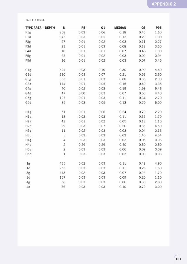
101

TABLE 7 Contd.


F1d 975 0.03 0.05 0.13 0.29 1.00

F3g 27 0.01 0.02 0.03 0.11 0.27

F3d 23 0.01 0.03 0.08 0.18 3.50

F4d 10 0.01 0.01 0.07 0.48 1.00

F5g 25 0.01 0.02 0.03 0.09 0.94

F5d 16 0.01 0.02 0.03 0.07 0.45

G1g 594 0.03 0.10 0.30 0.90 4.50

G1d 630 0.03 0.07 0.21 0.53 2.60

G3g 353 0.01 0.03 0.08 0.35 2.30

G3d 174 0.01 0.05 0.15 0.40 3.35

G4g 40 0.02 0.03 0.19 1.93 9.46

G4d 47 0.00 0.03 0.07 0.60 4.40

G5g 127 0.01 0.03 0.11 0.34 2.70

G5d 35 0.03 0.05 0.13 0.70 5.00

H1g 51 0.01 0.06 0.24 0.70 2.20

H1d 18 0.03 0.03 0.11 0.35 1.70

H2g 42 0.01 0.02 0.05 0.13 1.10

H2d 29 0.03 0.07 0.20 0.36 4.50

H3g 11 0.02 0.03 0.03 0.04 0.16

H3d 5 0.03 0.03 0.03 1.40 4.54

H4g 4 0.03 0.03 0.03 0.05 0.05

H4d 2 0.29 0.29 0.40 0.50 0.50

H5g 2 0.03 0.03 0.06 0.09 0.09

H5d 1 0.03 0.03 0.03 0.03 0.03

I1g 435 0.02 0.03 0.11 0.42 4.90

I1d 253 0.03 0.03 0.11 0.26 1.60

I3g 443 0.02 0.03 0.07 0.24 1.70

I3d 157 0.03 0.03 0.09 0.20 1.10

I4g 56 0.03 0.03 0.06 0.30 2.80

I4d 36 0.03 0.03 0.10 0.79 3.00

APPENDIX 2

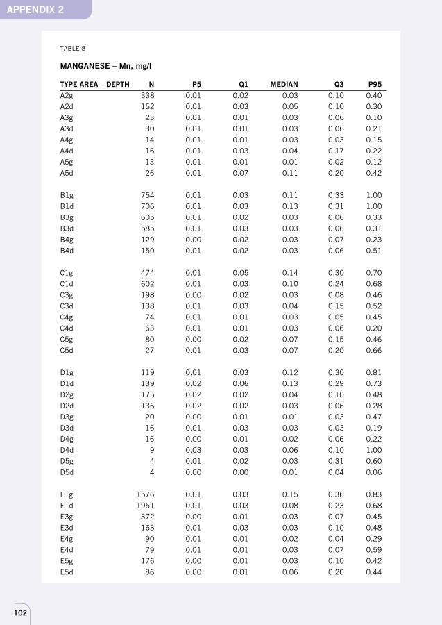
102

TABLE 8

MANGANESE – Mn, mg/l


A2d 152 0.01 0.03 0.05 0.10 0.30

A3g 23 0.01 0.01 0.03 0.06 0.10

A3d 30 0.01 0.01 0.03 0.06 0.21

A4g 14 0.01 0.01 0.03 0.03 0.15

A4d 16 0.01 0.03 0.04 0.17 0.22

A5g 13 0.01 0.01 0.01 0.02 0.12

A5d 26 0.01 0.07 0.11 0.20 0.42

B1g 754 0.01 0.03 0.11 0.33 1.00

B1d 706 0.01 0.03 0.13 0.31 1.00

B3g 605 0.01 0.02 0.03 0.06 0.33

B3d 585 0.01 0.03 0.03 0.06 0.31

B4g 129 0.00 0.02 0.03 0.07 0.23

B4d 150 0.01 0.02 0.03 0.06 0.51

C1g 474 0.01 0.05 0.14 0.30 0.70

C1d 602 0.01 0.03 0.10 0.24 0.68

C3g 198 0.00 0.02 0.03 0.08 0.46

C3d 138 0.01 0.03 0.04 0.15 0.52

C4g 74 0.01 0.01 0.03 0.05 0.45

C4d 63 0.01 0.01 0.03 0.06 0.20

C5g 80 0.00 0.02 0.07 0.15 0.46

C5d 27 0.01 0.03 0.07 0.20 0.66

D1g 119 0.01 0.03 0.12 0.30 0.81

D1d 139 0.02 0.06 0.13 0.29 0.73

D2g 175 0.02 0.02 0.04 0.10 0.48

D2d 136 0.02 0.02 0.03 0.06 0.28

D3g 20 0.00 0.01 0.01 0.03 0.47

D3d 16 0.01 0.03 0.03 0.03 0.19

D4g 16 0.00 0.01 0.02 0.06 0.22

D4d 9 0.03 0.03 0.06 0.10 1.00

D5g 4 0.01 0.02 0.03 0.31 0.60

D5d 4 0.00 0.00 0.01 0.04 0.06

E1g 1576 0.01 0.03 0.15 0.36 0.83

E1d 1951 0.01 0.03 0.08 0.23 0.68

E3g 372 0.00 0.01 0.03 0.07 0.45

E3d 163 0.01 0.03 0.03 0.10 0.48

E4g 90 0.01 0.01 0.02 0.04 0.29

E4d 79 0.01 0.01 0.03 0.07 0.59

E5g 176 0.00 0.01 0.03 0.10 0.42

E5d 86 0.00 0.01 0.06 0.20 0.44

APPENDIX 2

103

TABLE 8 Contd.


F1d 975 0.02 0.03 0.06 0.12 0.31

F3g 27 0.01 0.01 0.01 0.03 0.15

F3d 23 0.01 0.01 0.03 0.12 0.31

F4d 10 0.01 0.01 0.02 0.03 0.05

F5g 25 0.01 0.01 0.01 0.03 0.45

F5d 16 0.01 0.01 0.01 0.02 0.20

G1g 587 0.01 0.03 0.08 0.20 0.54

G1d 626 0.01 0.03 0.07 0.16 0.44

G3g 325 0.00 0.01 0.02 0.03 0.20

G3d 167 0.01 0.01 0.03 0.05 0.38

G4g 37 0.00 0.01 0.03 0.10 0.30

G4d 43 0.00 0.02 0.03 0.10 0.29

G5g 121 0.00 0.01 0.02 0.07 0.27

G5d 31 0.01 0.01 0.03 0.09 0.37

H1g 51 0.00 0.03 0.06 0.23 0.50

H1d 18 0.01 0.03 0.03 0.09 0.37

H2g 42 0.00 0.01 0.02 0.07 0.60

H2d 29 0.01 0.03 0.03 0.08 1.40

H3g 11 0.00 0.01 0.01 0.01 0.02

H3d 5 0.01 0.01 0.03 0.36 0.95

H4g 4 0.01 0.01 0.02 0.02 0.03

H4d 2 0.03 0.03 0.03 0.03 0.03

H5g 2 0.01 0.01 0.02 0.03 0.03

H5d 1 0.03 0.03 0.03 0.03 0.03

I1g 390 0.00 0.03 0.05 0.21 0.70

I1d 239 0.01 0.03 0.07 0.18 0.60

I3g 362 0.01 0.01 0.03 0.05 0.27

I3d 104 0.01 0.01 0.03 0.04 0.30

I4g 48 0.01 0.01 0.03 0.05 0.64

I4d 30 0.01 0.02 0.03 0.05 0.30

APPENDIX 2

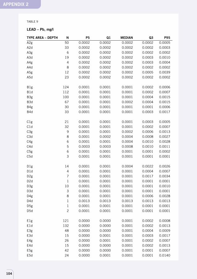
104

TABLE 9

LEAD – Pb, mg/l


A2d 33 0.0002 0.0002 0.0002 0.0002 0.0003

A3g 6 0.0002 0.0002 0.0002 0.0002 0.0002

A3d 19 0.0002 0.0002 0.0002 0.0003 0.0010

A4g 4 0.0002 0.0002 0.0002 0.0003 0.0004

A4d 8 0.0002 0.0002 0.0002 0.0002 0.0002

A5g 12 0.0002 0.0002 0.0002 0.0005 0.0039

A5d 23 0.0002 0.0002 0.0002 0.0002 0.0002

B1g 124 0.0001 0.0001 0.0001 0.0002 0.0006

B1d 112 0.0001 0.0001 0.0001 0.0002 0.0007

B3g 100 0.0001 0.0001 0.0001 0.0004 0.0015

B3d 67 0.0001 0.0001 0.0002 0.0004 0.0015

B4g 30 0.0001 0.0001 0.0001 0.0001 0.0006

B4d 33 0.0001 0.0001 0.0001 0.0003 0.0017

C1g 21 0.0001 0.0001 0.0001 0.0003 0.0005

C1d 32 0.0001 0.0001 0.0001 0.0002 0.0007

C3g 9 0.0001 0.0001 0.0002 0.0006 0.0013

C3d 8 0.0001 0.0002 0.0004 0.0008 0.0027

C4g 6 0.0001 0.0001 0.0004 0.0010 0.0028

C4d 5 0.0003 0.0003 0.0008 0.0010 0.0011

C5g 6 0.0001 0.0001 0.0001 0.0001 0.0002

C5d 3 0.0001 0.0001 0.0001 0.0001 0.0001

D1g 14 0.0001 0.0001 0.0004 0.0022 0.0026

D1d 4 0.0001 0.0001 0.0001 0.0004 0.0007

D2g 7 0.0001 0.0001 0.0001 0.0017 0.0034

D2d 1 0.0001 0.0001 0.0001 0.0001 0.0001

D3g 10 0.0001 0.0001 0.0001 0.0001 0.0010

D3d 3 0.0001 0.0001 0.0001 0.0001 0.0001

D4g 8 0.0001 0.0001 0.0001 0.0006 0.0028

D4d 1 0.0013 0.0013 0.0013 0.0013 0.0013

D5g 1 0.0001 0.0001 0.0001 0.0001 0.0001

D5d 2 0.0001 0.0001 0.0001 0.0001 0.0001

E1g 121 0.0000 0.0000 0.0001 0.0002 0.0008

E1d 132 0.0000 0.0000 0.0001 0.0002 0.0013

E3g 48 0.0000 0.0000 0.0001 0.0004 0.0009

E3d 15 0.0000 0.0001 0.0001 0.0003 0.0017

E4g 26 0.0000 0.0001 0.0001 0.0002 0.0007

E4d 15 0.0000 0.0000 0.0001 0.0002 0.0013

E5g 42 0.0000 0.0000 0.0001 0.0001 0.0007

E5d 24 0.0000 0.0001 0.0001 0.0001 0.0140

APPENDIX 2

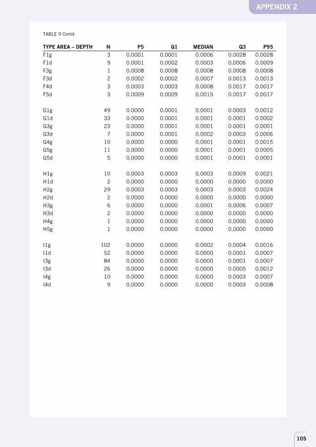
105

TABLE 9 Contd.


F1d 9 0.0001 0.0002 0.0003 0.0006 0.0009

F3g 1 0.0008 0.0008 0.0008 0.0008 0.0008

F3d 2 0.0002 0.0002 0.0007 0.0013 0.0013

F4d 3 0.0003 0.0003 0.0008 0.0017 0.0017

F5d 3 0.0009 0.0009 0.0015 0.0017 0.0017

G1g 49 0.0000 0.0001 0.0001 0.0003 0.0012

G1d 33 0.0000 0.0001 0.0001 0.0001 0.0002

G3g 23 0.0000 0.0001 0.0001 0.0001 0.0001

G3d 7 0.0000 0.0001 0.0002 0.0003 0.0006

G4g 10 0.0000 0.0000 0.0001 0.0001 0.0015

G5g 11 0.0000 0.0000 0.0001 0.0001 0.0005

G5d 5 0.0000 0.0000 0.0001 0.0001 0.0001

H1g 10 0.0003 0.0003 0.0003 0.0009 0.0021

H1d 2 0.0000 0.0000 0.0000 0.0000 0.0000

H2g 29 0.0003 0.0003 0.0003 0.0003 0.0024

H2d 2 0.0000 0.0000 0.0000 0.0000 0.0000

H3g 6 0.0000 0.0000 0.0001 0.0006 0.0007

H3d 2 0.0000 0.0000 0.0000 0.0000 0.0000

H4g 1 0.0000 0.0000 0.0000 0.0000 0.0000

H5g 1 0.0000 0.0000 0.0000 0.0000 0.0000

I1g 102 0.0000 0.0000 0.0002 0.0004 0.0016

I1d 52 0.0000 0.0000 0.0000 0.0001 0.0007

I3g 84 0.0000 0.0000 0.0000 0.0001 0.0007

I3d 26 0.0000 0.0000 0.0000 0.0005 0.0012

I4g 10 0.0000 0.0000 0.0000 0.0003 0.0007

I4d 9 0.0000 0.0000 0.0000 0.0003 0.0008

APPENDIX 2

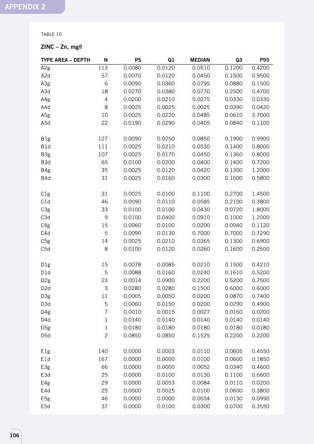
106

TABLE 10

ZINC – Zn, mg/l


A2d 57 0.0070 0.0120 0.0450 0.1500 0.9500

A3g 6 0.0090 0.0360 0.0795 0.0880 0.1500

A3d 18 0.0270 0.0380 0.0770 0.2500 0.4700

A4g 4 0.0200 0.0210 0.0275 0.0330 0.0330

A4d 8 0.0025 0.0025 0.0025 0.0390 0.0420

A5g 10 0.0025 0.0220 0.0485 0.0610 3.7000

A5d 22 0.0190 0.0290 0.0405 0.0840 0.1100

B1g 127 0.0090 0.0250 0.0850 0.1900 0.9900

B1d 111 0.0025 0.0210 0.0530 0.1400 0.8000

B3g 107 0.0025 0.0170 0.0450 0.1360 0.8000

B3d 65 0.0100 0.0200 0.0400 0.1400 0.7200

B4g 35 0.0025 0.0120 0.0420 0.1300 1.2000

B4d 31 0.0025 0.0160 0.0300 0.1500 0.5800

C1g 31 0.0025 0.0100 0.1100 0.2700 1.4500

C1d 46 0.0090 0.0110 0.0585 0.2100 0.3800

C3g 33 0.0100 0.0100 0.0430 0.0720 1.8000

C3d 9 0.0100 0.0400 0.0910 0.1000 1.2000

C4g 15 0.0060 0.0100 0.0200 0.0940 0.1120

C4d 5 0.0090 0.0130 0.7000 0.7000 0.7290

C5g 14 0.0025 0.0210 0.0365 0.1300 0.6900

C5d 8 0.0100 0.0120 0.0260 0.1600 0.2500

D1g 15 0.0078 0.0085 0.0210 0.1500 0.4210

D1d 5 0.0088 0.0160 0.0240 0.1610 0.5200

D2g 23 0.0014 0.0900 0.2200 0.5200 0.7500

D2d 3 0.0280 0.0280 0.1500 0.6000 0.6000

D3g 11 0.0005 0.0050 0.0200 0.0870 0.7400

D3d 5 0.0060 0.0150 0.0200 0.0290 0.4900

D4g 7 0.0010 0.0015 0.0027 0.0160 0.0200

D4d 1 0.0140 0.0140 0.0140 0.0140 0.0140

D5g 1 0.0180 0.0180 0.0180 0.0180 0.0180

D5d 2 0.0850 0.0850 0.1525 0.2200 0.2200

E1g 140 0.0000 0.0003 0.0110 0.0605 0.4550

E1d 167 0.0000 0.0000 0.0100 0.0600 0.1850

E3g 66 0.0000 0.0000 0.0052 0.0340 0.4600

E3d 25 0.0000 0.0100 0.0130 0.1100 0.6600

E4g 29 0.0000 0.0053 0.0084 0.0110 0.0200

E4d 25 0.0000 0.0025 0.0100 0.0600 0.3800

E5g 46 0.0000 0.0000 0.0034 0.0130 0.0990

E5d 37 0.0000 0.0100 0.0300 0.0700 0.3550

APPENDIX 2

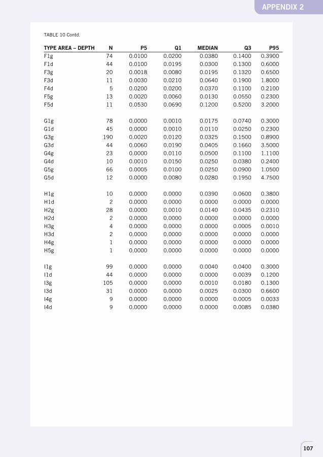
107

TABLE 10 Contd.


F1d 44 0.0100 0.0195 0.0300 0.1300 0.6000

F3g 20 0.0018 0.0080 0.0195 0.1320 0.6500

F3d 11 0.0030 0.0210 0.0640 0.1900 1.8000

F4d 5 0.0200 0.0200 0.0370 0.1100 0.2100

F5g 13 0.0020 0.0060 0.0130 0.0550 0.2300

F5d 11 0.0530 0.0690 0.1200 0.5200 3.2000

G1g 78 0.0000 0.0010 0.0175 0.0740 0.3000

G1d 45 0.0000 0.0010 0.0110 0.0250 0.2300

G3g 190 0.0020 0.0120 0.0325 0.1500 0.8900

G3d 44 0.0060 0.0190 0.0405 0.1660 3.5000

G4g 23 0.0000 0.0110 0.0500 0.1100 1.1100

G4d 10 0.0010 0.0150 0.0250 0.0380 0.2400

G5g 66 0.0005 0.0100 0.0250 0.0900 1.0500

G5d 12 0.0000 0.0080 0.0280 0.1950 4.7500

H1g 10 0.0000 0.0000 0.0390 0.0600 0.3800

H1d 2 0.0000 0.0000 0.0000 0.0000 0.0000

H2g 28 0.0000 0.0010 0.0140 0.0435 0.2310

H2d 2 0.0000 0.0000 0.0000 0.0000 0.0000

H3g 4 0.0000 0.0000 0.0000 0.0005 0.0010

H3d 2 0.0000 0.0000 0.0000 0.0000 0.0000

H4g 1 0.0000 0.0000 0.0000 0.0000 0.0000

H5g 1 0.0000 0.0000 0.0000 0.0000 0.0000

I1g 99 0.0000 0.0000 0.0040 0.0400 0.3000

I1d 44 0.0000 0.0000 0.0000 0.0039 0.1200

I3g 105 0.0000 0.0000 0.0010 0.0180 0.1300

I3d 31 0.0000 0.0000 0.0025 0.0300 0.6600

I4g 9 0.0000 0.0000 0.0000 0.0005 0.0033

I4d 9 0.0000 0.0000 0.0000 0.0085 0.0380

APPENDIX 2

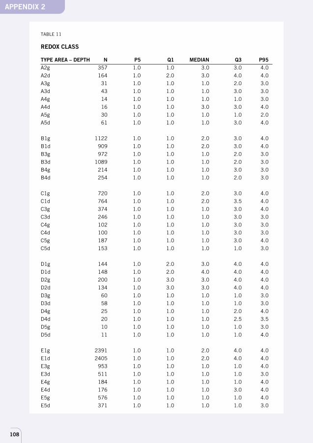
108

TABLE 11

REDOX CLASS


A2d 164 1.0 2.0 3.0 4.0 4.0

A3g 31 1.0 1.0 1.0 2.0 3.0

A3d 43 1.0 1.0 1.0 3.0 3.0

A4g 14 1.0 1.0 1.0 1.0 3.0

A4d 16 1.0 1.0 3.0 3.0 4.0

A5g 30 1.0 1.0 1.0 1.0 2.0

A5d 61 1.0 1.0 1.0 3.0 4.0

B1g 1122 1.0 1.0 2.0 3.0 4.0

B1d 909 1.0 1.0 2.0 3.0 4.0

B3g 972 1.0 1.0 1.0 2.0 3.0

B3d 1089 1.0 1.0 1.0 2.0 3.0

B4g 214 1.0 1.0 1.0 3.0 3.0

B4d 254 1.0 1.0 1.0 2.0 3.0

C1g 720 1.0 1.0 2.0 3.0 4.0

C1d 764 1.0 1.0 2.0 3.5 4.0

C3g 374 1.0 1.0 1.0 3.0 4.0

C3d 246 1.0 1.0 1.0 3.0 3.0

C4g 102 1.0 1.0 1.0 3.0 3.0

C4d 100 1.0 1.0 1.0 3.0 3.0

C5g 187 1.0 1.0 1.0 3.0 4.0

C5d 153 1.0 1.0 1.0 1.0 3.0

D1g 144 1.0 2.0 3.0 4.0 4.0

D1d 148 1.0 2.0 4.0 4.0 4.0

D2g 200 1.0 3.0 3.0 4.0 4.0

D2d 134 1.0 3.0 3.0 4.0 4.0

D3g 60 1.0 1.0 1.0 1.0 3.0

D3d 58 1.0 1.0 1.0 1.0 3.0

D4g 25 1.0 1.0 1.0 2.0 4.0

D4d 20 1.0 1.0 1.0 2.5 3.5

D5g 10 1.0 1.0 1.0 1.0 3.0

D5d 11 1.0 1.0 1.0 1.0 4.0

E1g 2391 1.0 1.0 2.0 4.0 4.0

E1d 2405 1.0 1.0 2.0 4.0 4.0

E3g 953 1.0 1.0 1.0 1.0 4.0

E3d 511 1.0 1.0 1.0 1.0 3.0

E4g 184 1.0 1.0 1.0 1.0 4.0

E4d 176 1.0 1.0 1.0 3.0 4.0

E5g 576 1.0 1.0 1.0 1.0 4.0

E5d 371 1.0 1.0 1.0 1.0 3.0

APPENDIX 2

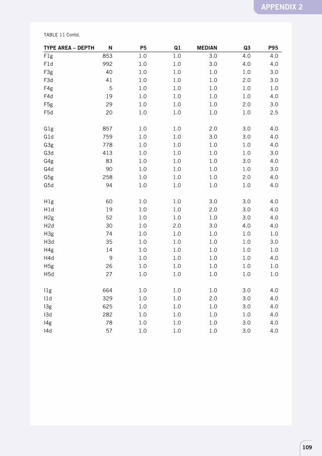
109

TABLE 11 Contd.


F1d 992 1.0 1.0 3.0 4.0 4.0

F3g 40 1.0 1.0 1.0 1.0 3.0

F3d 41 1.0 1.0 1.0 2.0 3.0

F4g 5 1.0 1.0 1.0 1.0 1.0

F4d 19 1.0 1.0 1.0 1.0 4.0

F5g 29 1.0 1.0 1.0 2.0 3.0

F5d 20 1.0 1.0 1.0 1.0 2.5

G1g 857 1.0 1.0 2.0 3.0 4.0

G1d 759 1.0 1.0 3.0 3.0 4.0

G3g 778 1.0 1.0 1.0 1.0 4.0

G3d 413 1.0 1.0 1.0 1.0 3.0

G4g 83 1.0 1.0 1.0 3.0 4.0

G4d 90 1.0 1.0 1.0 1.0 3.0

G5g 258 1.0 1.0 1.0 2.0 4.0

G5d 94 1.0 1.0 1.0 1.0 4.0

H1g 60 1.0 1.0 3.0 3.0 4.0

H1d 19 1.0 1.0 2.0 3.0 4.0

H2g 52 1.0 1.0 1.0 3.0 4.0

H2d 30 1.0 2.0 3.0 4.0 4.0

H3g 74 1.0 1.0 1.0 1.0 1.0

H3d 35 1.0 1.0 1.0 1.0 3.0

H4g 14 1.0 1.0 1.0 1.0 1.0

H4d 9 1.0 1.0 1.0 1.0 4.0

H5g 26 1.0 1.0 1.0 1.0 1.0

H5d 27 1.0 1.0 1.0 1.0 1.0

I1g 664 1.0 1.0 1.0 3.0 4.0

I1d 329 1.0 1.0 2.0 3.0 4.0

I3g 625 1.0 1.0 1.0 3.0 4.0

I3d 282 1.0 1.0 1.0 1.0 4.0

I4g 78 1.0 1.0 1.0 3.0 4.0

I4d 57 1.0 1.0 1.0 3.0 4.0

APPENDIX 2

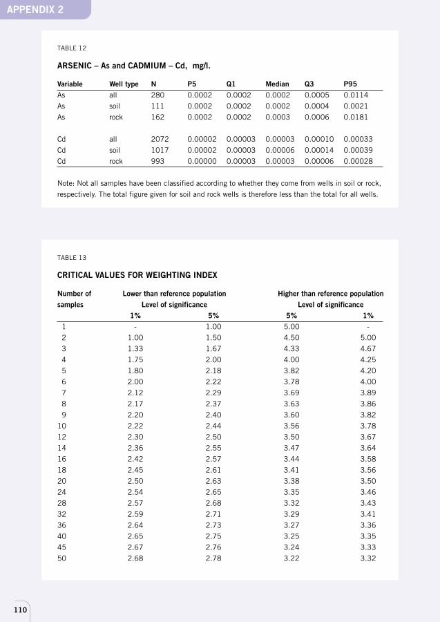
110

TABLE 12

ARSENIC – As and CADMIUM – Cd, mg/l.

Variable Well type N P5 Q1 Median Q3 P95As all 280 0.0002 0.0002 0.0002 0.0005 0.0114

As soil 111 0.0002 0.0002 0.0002 0.0004 0.0021

As rock 162 0.0002 0.0002 0.0003 0.0006 0.0181

Cd all 2072 0.00002 0.00003 0.00003 0.00010 0.00033

Cd soil 1017 0.00002 0.00003 0.00006 0.00014 0.00039

Cd rock 993 0.00000 0.00003 0.00003 0.00006 0.00028

Note: Not all samples have been classified according to whether they come from wells in soil or rock,

respectively. The total figure given for soil and rock wells is therefore less than the total for all wells.

TABLE 13

CRITICAL VALUES FOR WEIGHTING INDEX

Number of Lower than reference population Higher than reference populationsamples Level of significance Level of significance

1% 5% 5% 1% 1 - 1.00 5.00 -

2 1.00 1.50 4.50 5.00

3 1.33 1.67 4.33 4.67

4 1.75 2.00 4.00 4.25

5 1.80 2.18 3.82 4.20

6 2.00 2.22 3.78 4.00

7 2.12 2.29 3.69 3.89

8 2.17 2.37 3.63 3.86

9 2.20 2.40 3.60 3.82

10 2.22 2.44 3.56 3.78

12 2.30 2.50 3.50 3.67

14 2.36 2.55 3.47 3.64

16 2.42 2.57 3.44 3.58

18 2.45 2.61 3.41 3.56

20 2.50 2.63 3.38 3.50

24 2.54 2.65 3.35 3.46

28 2.57 2.68 3.32 3.43

32 2.59 2.71 3.29 3.41

36 2.64 2.73 3.27 3.36

40 2.65 2.75 3.25 3.35

45 2.67 2.76 3.24 3.33

50 2.68 2.78 3.22 3.32

APPENDIX 2

111

Example presentation of data

APPENDIX 3

An example of presentation of current condition, the ratio of alkalinity tosulphate deposition and deviation from the reference population. The de-viation test is used for the latter.

A municipality in central Sweden wishes to study alkalinity – risk of acidificationin shallow (<4 m) wells in moraine and deep (>4 m) excavated wells under cohe-sive soils. The municipality has sampled 10 wells in each environment.

One of the main aims is to ascertain whether alkalinity in municipal wellsdeviates from other areas of the country where conditions are comparable, ie, inthe same type areas. A deviation test is therefore made to see whether municipalalkalinity data deviates from reference population alkalinity data.

To do this, it will first be necessary to identify the reference populations.According to the regional classification of Sweden (see Figure 2, page 22), themunicipality is in region E. Shallow wells in moraine belong to groundwaterenvironment 3 as described on page 24 and deep wells under cohesive soils togroundwater environment 5. The analysis figures obtained are therefore classifiedas type area-depth E3g (shallow wells in moraine or fluvial outwash) and typearea-depth E5d (deep wells under cohesive soils), respectively, in Table 2 on page90.

The table shows type area populations divided according to percentiles. Mu-nicipal analysis figures are compared, one at a time, with the type area table.Classification, which is a way of showing how the municipal figure compareswith the distribution of concentrations in the type area population, is made inthe way described in the chapter on “Instructions for deviation test”. Note thatclass value 1 is used for the lowest relative values and class value 5 for the highest,regardless of whether low values are “good” or “bad”.

Weighting indixes are now computed as the mean of all individual class valu-es obtained. In our example, the municipality has only taken ten samples in eachtype area and well-depth class and these gave weighting indixes of 2.20 and 2.80,respectively. The significance of the weighting index obtained depends on thenumber of samples and the chosen level of significance as shown in Table 13 onpage 110. According to the table, alkalinity values for wells in moraine are signi-ficantly lower than those of the reference group at a significance level of 1 percent (critical value 2.22).

The inference is that the alkalinity of shallow wells in moraine in the munici-pality (assuming that those sampled are representative of this kind of well in themunicipality) is significantly higher than is generally the case in wells of thiskind in the central Swedish depression. The calculated risk that the observeddifference is due to random factors is just less than 1 per cent.

On the other hand, the weighting index for deep wells under cohesive soils

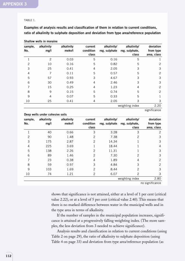
112

APPENDIX 3

Shallow wells in moraine

sample, alkalinity alkalinity current alkalinity/ alkalinity/ deviationNo. mg/l mekv/l condition reg. sulphate reg. sulphate, from type

class class area, class

1 2 0.03 5 0.16 5 1

2 10 0.16 5 0.82 5 2

3 25 0.41 4 2.05 3 3

4 7 0.11 5 0.57 5 2

5 57 0.93 3 4.67 3 3

6 30 0.49 4 2.46 3 3

7 15 0.25 4 1.23 4 2

8 9 0.15 5 0.74 5 2

9 4 0.07 5 0.33 5 1

10 25 0.41 4 2.05 3 3

weighting index 2.20significance

Deep wells under cohesive soils

sample, alkalinity alkalinity current alkalinity/ alkalinity/ deviationNo. mg/l mekv/l condition reg. sulphate reg. sulphate, from type

class class area, class

1 40 0.66 3 3.28 3 2

2 90 1.48 2 7.38 2 3

3 175 2.87 2 14.34 1 3

4 225 3.69 1 18.44 1 4

5 138 2.26 2 11.31 1 3

6 89 1.46 2 7.30 2 3

7 23 0.38 4 1.89 4 2

8 59 0.97 3 4.84 3 2

9 103 1.69 2 8.44 2 3

10 74 1.21 2 6.07 2 3

weighting index 2.80no significance

TABLE 1.

Examples of analysis results and classification of them in relation to current conditions,

ratio of alkalinity to sulphate deposition and deviation from type area/reference population

shows that significance is not attained, either at a level of 1 per cent (criticalvalue 2.22), or at a level of 5 per cent (critical value 2.40). This means thatthere is no marked difference between water in the municipal wells and inthe type area in terms of alkalinity.

If the number of samples in the municipal population increases, signifi-cance is attained at a progressively falling weighting index. (The more sam-ples, the less deviation from 3 needed to achieve significance).

Analysis results and classification in relation to current conditions (usingTable 2 on page 29), the ratio of alkalinity to sulphate deposition (usingTable 4 on page 33) and deviation from type area/reference population (as

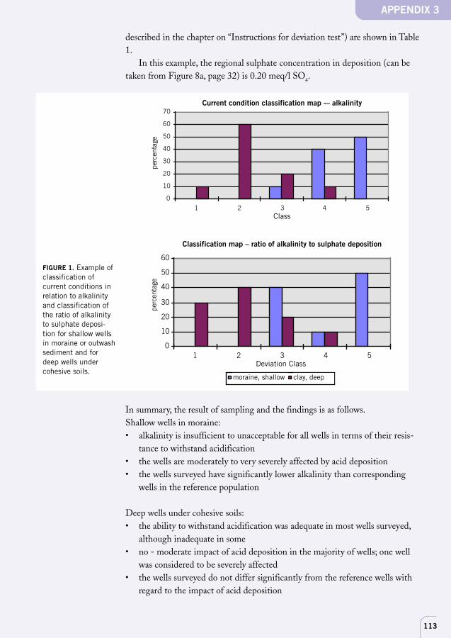
113

APPENDIX 3

described in the chapter on “Instructions for deviation test”) are shown in Table1.

In this example, the regional sulphate concentration in deposition (can betaken from Figure 8a, page 32) is 0.20 meq/l SO4.

In summary, the result of sampling and the findings is as follows.Shallow wells in moraine:• alkalinity is insufficient to unacceptable for all wells in terms of their resis-

tance to withstand acidification• the wells are moderately to very severely affected by acid deposition• the wells surveyed have significantly lower alkalinity than corresponding

wells in the reference population

Deep wells under cohesive soils:• the ability to withstand acidification was adequate in most wells surveyed,

although inadequate in some• no - moderate impact of acid deposition in the majority of wells; one well

was considered to be severely affected• the wells surveyed do not differ significantly from the reference wells with

regard to the impact of acid deposition

perc

enta

gepe

rcen

tage

Current condition classification map -– alkalinity

FIGURE 1. Example ofclassification ofcurrent conditions inrelation to alkalinityand classification ofthe ratio of alkalinityto sulphate deposi-tion for shallow wellsin moraine or outwashsediment and fordeep wells undercohesive soils.

Current condition classification map -– alkalinity

�

��

��

��

��

��

��

��

� � � � �

Classification map – ratio of alkalinity to sulphate deposition

Class

Class

moraine, shallow clay, deep

�

��

��

��

��

��

��

� � � � ��

�� moraine, shallow clay, deep

Deviation Class

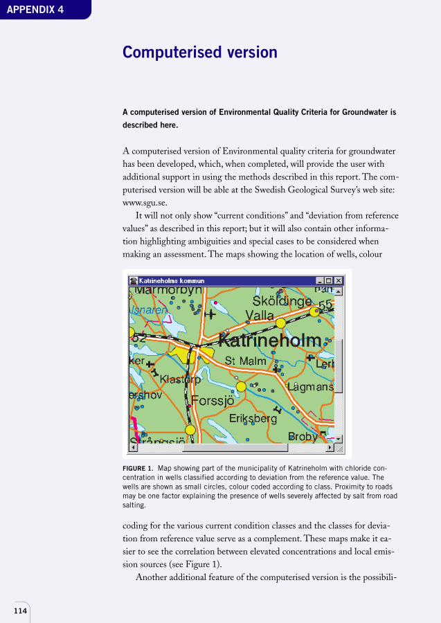
114

APPENDIX 4

Computerised version

A computerised version of Environmental Quality Criteria for Groundwater is

described here.

A computerised version of Environmental quality criteria for groundwaterhas been developed, which, when completed, will provide the user withadditional support in using the methods described in this report. The com-puterised version will be able at the Swedish Geological Survey’s web site:www.sgu.se.

It will not only show “current conditions” and “deviation from referencevalues” as described in this report; but it will also contain other informa-tion highlighting ambiguities and special cases to be considered whenmaking an assessment. The maps showing the location of wells, colour

coding for the various current condition classes and the classes for devia-tion from reference value serve as a complement. These maps make it ea-sier to see the correlation between elevated concentrations and local emis-sion sources (see Figure 1).

Another additional feature of the computerised version is the possibili-

FIGURE 1. Map showing part of the municipality of Katrineholm with chloride con-centration in wells classified according to deviation from the reference value. Thewells are shown as small circles, colour coded according to class. Proximity to roadsmay be one factor explaining the presence of wells severely affected by salt from roadsalting.

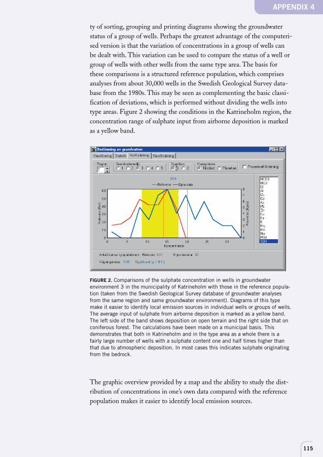
115

APPENDIX 4

ty of sorting, grouping and printing diagrams showing the groundwaterstatus of a group of wells. Perhaps the greatest advantage of the computeri-sed version is that the variation of concentrations in a group of wells canbe dealt with. This variation can be used to compare the status of a well orgroup of wells with other wells from the same type area. The basis forthese comparisons is a structured reference population, which comprisesanalyses from about 30,000 wells in the Swedish Geological Survey data-base from the 1980s. This may be seen as complementing the basic classi-fication of deviations, which is performed without dividing the wells intotype areas. Figure 2 showing the conditions in the Katrineholm region, theconcentration range of sulphate input from airborne deposition is markedas a yellow band.

FIGURE 2. Comparisons of the sulphate concentration in wells in groundwaterenvironment 3 in the municipality of Katrineholm with those in the reference popula-tion (taken from the Swedish Geological Survey database of groundwater analysesfrom the same region and same groundwater environment). Diagrams of this typemake it easier to identify local emission sources in individual wells or groups of wells.The average input of sulphate from airborne deposition is marked as a yellow band.The left side of the band shows deposition on open terrain and the right side that onconiferous forest. The calculations have been made on a municipal basis. Thisdemonstrates that both in Katrineholm and in the type area as a whole there is afairly large number of wells with a sulphate content one and half times higher thanthat due to atmospheric deposition. In most cases this indicates sulphate originatingfrom the bedrock.

The graphic overview provided by a map and the ability to study the dist-ribution of concentrations in one’s own data compared with the referencepopulation makes it easier to identify local emission sources.

116

APPENDIX 5

Alkalinity – risk of acidification

This appendix presents the choice of parameters used to describe

acidification status.

IntroductionIt is difficult to determine the exact natural state of groundwater in termsof alkalinity or pH.

The ratio of alkalinity to total hardness or the “acid ratio” has oftenbeen used in the past to determine the degree of acidification impact. Thereason is that natural weathering by carbonic acid (see equation 2 on page28) theoretically gives the same quantity of base cations (of which calciumand magnesium are the largest part = total hardness) as alkalinity.Weathering under the strongly acidic conditions existing after depositionof acidifying compounds instead produces twice as many base cations asthe quantity of alkalinity. Instead of a 1:1 relationship between alkalinityand base cations, a 1:2 relationship occurs. (Bicarbonate ions make up themain part of what is normally termed the “buffering capacity” or alkalinityof the water.)

An attempt to estimate the margin of error when usingalkalinity/total hardness to describe acidification impactThe ratio and the difference may be distorted by factors other than acidifi-cation.The most important are:1. Ion exchange caused by chloride or nitrate2. Oxidation of sulphur in the soil3. The fact that the acid ratio is not proportional to the acidification im-

pact. This ratio may instead be expected to be greater at the beginningof an acidification process owing to greater availability of exchangeablecalcium and magnesium ions

4. Deposition of calcium and magnesium and weathering of sodium5. Other factors

The reasons become clear if we take the ionic balance into account, ie, thefact that the number of negatively charged ions (anions) is always equal tothe number of positively charged ions (cations) in the water. This meansthat all changes that increase or reduce the concentration of anions arecoupled with equally great changes in the concentration of cations. The

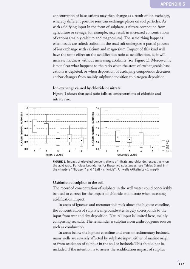
117

APPENDIX 5

concentration of base cations may then change as a result of ion exchange,whereby different positive ions can exchange places on soil particles. Aswith acidifying input in the form of sulphate, a nitrate compound fromagriculture or sewage, for example, may result in increased concentrationsof cations (mainly calcium and magnesium). The same thing happenswhen roads are salted: sodium in the road salt undergoes a partial processof ion exchange with calcium and magnesium. Impact of this kind willhave the same effect on the acidification ratio as acidification, ie, it willincrease hardness without increasing alkalinity (see Figure 1). Moreover, itis not clear what happens to the ratio when the store of exchangeable basecations is depleted, or when deposition of acidifying compounds decreasesand/or changes from mainly sulphur deposition to nitrogen deposition.

Ion exchange caused by chloride or nitrateFigure 1 shows that acid ratio falls as concentrations of chloride andnitrate rise.

Oxidation of sulphur in the soilThe recorded concentration of sulphate in the well water could conceivablybe used to correct for the impact of chloride and nitrate when assessingacidification impact.

In areas of igneous and metamorphic rock above the highest coastline,the concentration of sulphate in groundwater largely corresponds to theinput from wet and dry deposition. Natural input is limited here, mainlycomprising sea salts. The remainder is sulphur from anthropogenic sourcessuch as combustion.

In areas below the highest coastline and areas of sedimentary bedrock,many wells are severely affected by sulphate input, either of marine originor from oxidation of sulphur in the soil or bedrock. This should not beincluded if the intention is to assess the acidification impact of sulphur

FIGURE 1. Impact of elevated concentrations of nitrate and chloride, respectively, onthe acid ratio. For class boundaries for these two substances, see Tables 5 and 8 inthe chapters “Nitrogen” and “Salt - chloride”. All wells (Alkalinity <1 meq/l)

NITRATE CLASS

ALK

ALI

NIT

Y/TO

TAL

HA

RD

NE

SS

ALK

ALI

NIT

Y/TO

TAL

HA

RD

NE

SS

CHLORIDE CLASSNITRATE CLASS

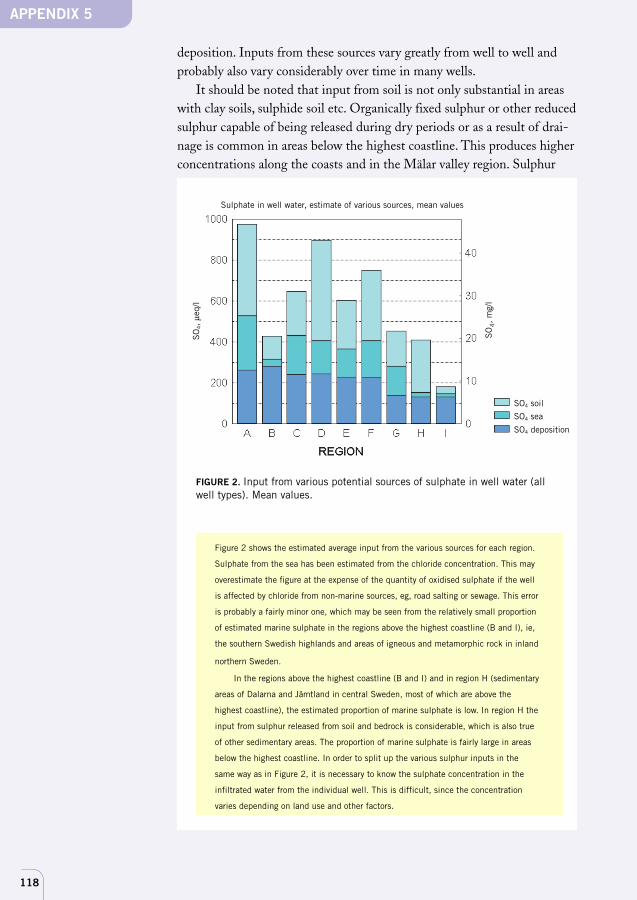
118

deposition. Inputs from these sources vary greatly from well to well andprobably also vary considerably over time in many wells.

It should be noted that input from soil is not only substantial in areaswith clay soils, sulphide soil etc. Organically fixed sulphur or other reducedsulphur capable of being released during dry periods or as a result of drai-nage is common in areas below the highest coastline. This produces higherconcentrations along the coasts and in the Mälar valley region. Sulphur

APPENDIX 5

FIGURE 2. Input from various potential sources of sulphate in well water (allwell types). Mean values.

Figure 2 shows the estimated average input from the various sources for each region.

Sulphate from the sea has been estimated from the chloride concentration. This may

overestimate the figure at the expense of the quantity of oxidised sulphate if the well

is affected by chloride from non-marine sources, eg, road salting or sewage. This error

is probably a fairly minor one, which may be seen from the relatively small proportion

of estimated marine sulphate in the regions above the highest coastline (B and I), ie,

the southern Swedish highlands and areas of igneous and metamorphic rock in inland

northern Sweden.

In the regions above the highest coastline (B and I) and in region H (sedimentary

areas of Dalarna and Jämtland in central Sweden, most of which are above the

highest coastline), the estimated proportion of marine sulphate is low. In region H the

input from sulphur released from soil and bedrock is considerable, which is also true

of other sedimentary areas. The proportion of marine sulphate is fairly large in areas

below the highest coastline. In order to split up the various sulphur inputs in the

same way as in Figure 2, it is necessary to know the sulphate concentration in the

infiltrated water from the individual well. This is difficult, since the concentration

varies depending on land use and other factors.

SO4 deposition

SO4 sea

SO4 soil

SO

4,

µeq/

lSulphate in well water, estimate of various sources, mean values

SO

4, m

g/l

119

concentrations are also higher in areas of sulphide mineralisation than insurrounding areas.

Input of marine sulphate is accompanied by base cations and is notacidifying, unlike deposition of sulphate from combustion processes etcand oxidation of sulphur in soil.

The fact that the acid ratio is not proportional to the acidification impactbut may instead be expected to be greater at the beginning of an acidifica-tion process owing to greater availability of exchangeable calcium andmagnesium ionsMuch of the shift in the acid ratio at the beginning of an acidificationprocess results from the increase in total hardness when calcium and mag-nesium are displaced from soil particles by hydrogen (and aluminium)ions. This displacement can be expected to lessen even where the acidifica-tion load is constant because the store of exchangeable base cations is dep-leted. In areas experiencing a peak of acidification impact, eg, Sweden, it isnot certain which direction the ratio will take. It is difficult to say howmuch uncertainty will be introduced by using the acid ratio because manyother factors are involved, eg, the original size of the cations in storage andthe size of the acidification load compared with weathering. The objectionto using the ratio because of this doubt is a matter of principle. It would beunfortunate if a constant acidification load were to be viewed as a decli-ning load.

Airborn deposition of calcium and magnesium and sodiumfrom weatheringAnother factor hindering the use of the ratio of alkalinity to total hardnessis that in naturally very ion-weak groundwaters a significant proportion ofcalcium and magnesium in groundwater may derive directly from deposi-tion. A further factor is that in very shallow groundwater, sodium byweathering is fairly significant. Since these two factors tend to cancel eachother out, the effect on the ratio is less, however. But there may be a greatimpact on individual wells owing to differing deposition or mineralogy. Itshould be stressed that it is essential to classify this group of wells correctly,since they are the water sources most sensitive to acidification.

Other factorsThe arguments above principally take account of factors causing displace-ment of calcium and magnesium. There are many other possibilities, ho-wever. If the soil is acid, input of salt, for example, may produce a directincrease in the quantity of hydrogen ions in the water phase, which maypossibly be involved in ion exchange or cause weathering further down inthe soil. Absorption of nutrients by plants often causes soil acidification.

APPENDIX 5

120

These processes, which are at least partly influenced by nitrogen availabili-ty, have a great impact on the soil in a given area and hence also on thegroundwater. These and many other factors affect the acid ratio and, itmight be mentioned, also the actual acidification impact on the groundwa-ter. This has not been dealt with here, however.

General comments on use of the acid ratio and the assessmentmethod proposed hereAs may be seen from the above, the acid ratio is heavily influenced by anumber of factors. It is difficult to ascertain what part of acidification im-pact derives from deposition and what is due to other causes in a givencase. The inclusion of total hardness and alkalinity in the ratio might besaid to ensure that a large proportion of the chemical constituents of thewater are covered.

A new concept has been developed for use in this Groundwater reportas a way of circumventing the difficulties of using the ratio of alkalinity tototal hardness. The new method is to compare the residual buffering capa-city of the water against acidification (its alkalinity) with the load in theform of sulphur deposition.

The problem of the influence of other types of impact lessens usingthis approach. The assessment is rough but comparatively transparent.The alkalinity of well water is compared directly with the acidificationload. Since the alkalinity of the water results from a number of processes,the alkalinity created by weathering has been partially used to neutraliseacid deposition, biological acidification and other soil processes such asoxidation of sulphur. Extensive ion exchange renders it impossible to esti-mate how great alkalinity would have been without the acid deposition.The extent to which the alkalinity of the water has already been affectedby acidification is not calculated. Hence, it is the amount of alkalinity thatis compared with the amount of the acid deposition. Acceptance of thiswill make assessment easier.

It has been found that even if all wells have been affected by acid depo-sition, the alkalinity of water in most of them is so high compared with thedeposition that the acidification impact on the water is negligible. Thewells that have been severely affected by acid deposition can also be defini-tely identified.

APPENDIX 5

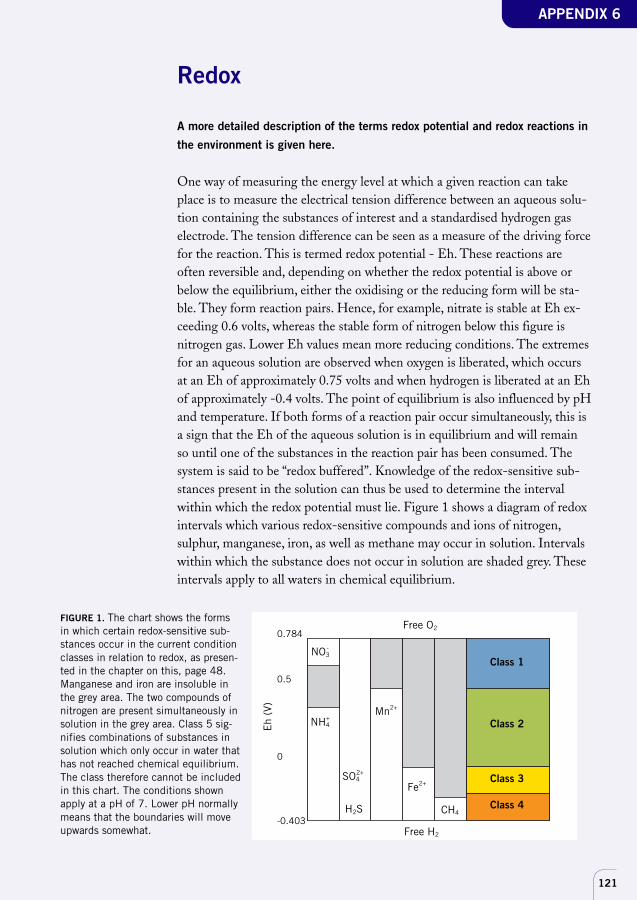
121

Redox

A more detailed description of the terms redox potential and redox reactions in

the environment is given here.

One way of measuring the energy level at which a given reaction can takeplace is to measure the electrical tension difference between an aqueous solu-tion containing the substances of interest and a standardised hydrogen gaselectrode. The tension difference can be seen as a measure of the driving forcefor the reaction. This is termed redox potential - Eh. These reactions areoften reversible and, depending on whether the redox potential is above orbelow the equilibrium, either the oxidising or the reducing form will be sta-ble. They form reaction pairs. Hence, for example, nitrate is stable at Eh ex-ceeding 0.6 volts, whereas the stable form of nitrogen below this figure isnitrogen gas. Lower Eh values mean more reducing conditions. The extremesfor an aqueous solution are observed when oxygen is liberated, which occursat an Eh of approximately 0.75 volts and when hydrogen is liberated at an Ehof approximately -0.4 volts. The point of equilibrium is also influenced by pHand temperature. If both forms of a reaction pair occur simultaneously, this isa sign that the Eh of the aqueous solution is in equilibrium and will remainso until one of the substances in the reaction pair has been consumed. Thesystem is said to be “redox buffered”. Knowledge of the redox-sensitive sub-stances present in the solution can thus be used to determine the intervalwithin which the redox potential must lie. Figure 1 shows a diagram of redoxintervals which various redox-sensitive compounds and ions of nitrogen,sulphur, manganese, iron, as well as methane may occur in solution. Intervalswithin which the substance does not occur in solution are shaded grey. Theseintervals apply to all waters in chemical equilibrium.

APPENDIX 6

FIGURE 1. The chart shows the formsin which certain redox-sensitive sub-stances occur in the current conditionclasses in relation to redox, as presen-ted in the chapter on this, page 48.Manganese and iron are insoluble inthe grey area. The two compounds ofnitrogen are present simultaneously insolution in the grey area. Class 5 sig-nifies combinations of substances insolution which only occur in water thathas not reached chemical equilibrium.The class therefore cannot be includedin this chart. The conditions shownapply at a pH of 7. Lower pH normallymeans that the boundaries will moveupwards somewhat. Free H2

Free O2

Class 1

Class 2

Class 3

Class 4

0.784

0.5

0

-0.403

Eh

(V)

NO3-

NH4+

CH4

SO42+

Mn2+

Fe2+

H2S

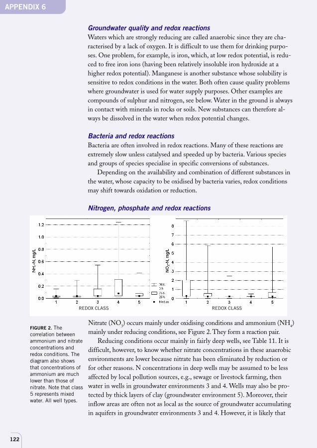
122

Groundwater quality and redox reactionsWaters which are strongly reducing are called anaerobic since they are cha-racterised by a lack of oxygen. It is difficult to use them for drinking purpo-ses. One problem, for example, is iron, which, at low redox potential, is redu-ced to free iron ions (having been relatively insoluble iron hydroxide at ahigher redox potential). Manganese is another substance whose solubility issensitive to redox conditions in the water. Both often cause quality problemswhere groundwater is used for water supply purposes. Other examples arecompounds of sulphur and nitrogen, see below. Water in the ground is alwaysin contact with minerals in rocks or soils. New substances can therefore al-ways be dissolved in the water when redox potential changes.

Bacteria and redox reactionsBacteria are often involved in redox reactions. Many of these reactions areextremely slow unless catalysed and speeded up by bacteria. Various speciesand groups of species specialise in specific conversions of substances.

Depending on the availability and combination of different substances inthe water, whose capacity to be oxidised by bacteria varies, redox conditionsmay shift towards oxidation or reduction.

Nitrogen, phosphate and redox reactions

Nitrate (NO3) occurs mainly under oxidising conditions and ammonium (NH4)mainly under reducing conditions, see Figure 2. They form a reaction pair.

Reducing conditions occur mainly in fairly deep wells, see Table 11. It isdifficult, however, to know whether nitrate concentrations in these anaerobicenvironments are lower because nitrate has been eliminated by reduction orfor other reasons. N concentrations in deep wells may be assumed to be lessaffected by local pollution sources, e.g., sewage or livestock farming, thenwater in wells in groundwater environments 3 and 4. Wells may also be pro-tected by thick layers of clay (groundwater environment 5). Moreover, theirinflow areas are often not as local as the source of groundwater accumulatingin aquifers in groundwater environments 3 and 4. However, it is likely that

APPENDIX 6

FIGURE 2. Thecorrelation betweenammonium and nitrateconcentrations andredox conditions. Thediagram also showsthat concentrations ofammonium are muchlower than those ofnitrate. Note that class5 represents mixedwater. All well types.

REDOX CLASS REDOX CLASS

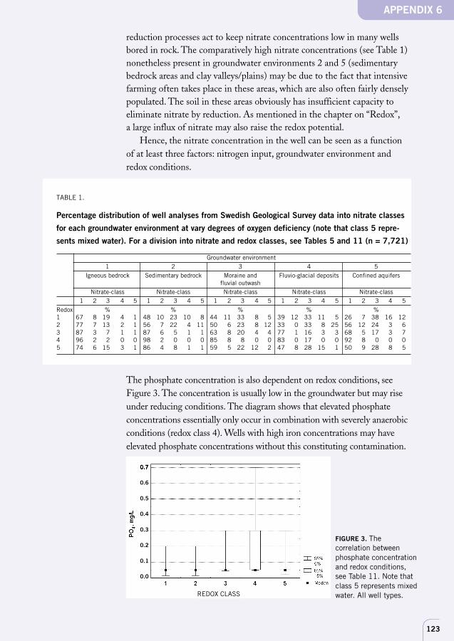
123

reduction processes act to keep nitrate concentrations low in many wellsbored in rock. The comparatively high nitrate concentrations (see Table 1)nonetheless present in groundwater environments 2 and 5 (sedimentarybedrock areas and clay valleys/plains) may be due to the fact that intensivefarming often takes place in these areas, which are also often fairly denselypopulated. The soil in these areas obviously has insufficient capacity toeliminate nitrate by reduction. As mentioned in the chapter on “Redox”,a large influx of nitrate may also raise the redox potential.

Hence, the nitrate concentration in the well can be seen as a functionof at least three factors: nitrogen input, groundwater environment andredox conditions.

TABLE 1.

Percentage distribution of well analyses from Swedish Geological Survey data into nitrate classes

for each groundwater environment at vary degrees of oxygen deficiency (note that class 5 repre-

sents mixed water). For a division into nitrate and redox classes, see Tables 5 and 11 (n = 7,721)



Nitrate-class Nitrate-class Nitrate-class Nitrate-class Nitrate-class1 2 3 4 5 1 2 3 4 5 1 2 3 4 5 1 2 3 4 5 1 2 3 4 5

Redox % % % % %1 67 8 19 4 1 48 10 23 10 8 44 11 33 8 5 39 12 33 11 5 26 7 38 16 122 77 7 13 2 1 56 7 22 4 11 50 6 23 8 12 33 0 33 8 25 56 12 24 3 63 87 3 7 1 1 87 6 5 1 1 63 8 20 4 4 77 1 16 3 3 68 5 17 3 74 96 2 2 0 0 98 2 0 0 0 85 8 8 0 0 83 0 17 0 0 92 8 0 0 05 74 6 15 3 1 86 4 8 1 1 59 5 22 12 2 47 8 28 15 1 50 9 28 8 5

The phosphate concentration is also dependent on redox conditions, seeFigure 3. The concentration is usually low in the groundwater but may riseunder reducing conditions. The diagram shows that elevated phosphateconcentrations essentially only occur in combination with severely anaerobicconditions (redox class 4). Wells with high iron concentrations may haveelevated phosphate concentrations without this constituting contamination.

APPENDIX 6

FIGURE 3. Thecorrelation betweenphosphate concentrationand redox conditions,see Table 11. Note thatclass 5 represents mixedwater. All well types.REDOX CLASS

0.7

0.6

0.5

0.4

0.3

0.2

0.1

0.0

124

Pesticides

A brief summary of studies of the occurrence of pesticides in groundwater is

given below. This is followed by a section describing the behaviour of pesti-

cides in soil and factors that increase the risk of leaching into groundwater.

The appendix concludes with a list of substances in an analysis package.

Some studies into the occurrence of pesticides in groundwaterFew surveys designed to detect the presence of pesticides in groundwaterhave yet been made. Those performed to date have usually been confined tolocations where groundwater contamination has been suspected.

For the period 1987–1996 there are 394 analyses of groundwater fromprivate wells in Malmöhus, Kristianstad and Gotland counties. Pesticideswere found in 43 per cent of the samples; a total of 21 substances were iden-tified. Targeted sampling explains the high proportion of contaminatedsamples.

In some cases, samples from public water supply sources have also revea-led low concentrations of pesticide residues. These surveys were performedat various locations throughout Sweden by the National Food Administra-tion. However, the concentrations are so low that the Administration doesnot consider them to pose a threat to health. The most commonly foundsubstances are used as weedkillers on uncultivated land.

The National Food Administration drinking water regulations stipulatethat drinking water from public water supplies must contain no demonstra-ble concentrations of pesticides.

The EC Drinking Water Directive sets a limit of 0.1 µg/l for each pesti-cide and 0.5 µg/l for total pesticides. Remedial action must be taken at theselevels.

Conditions governing pesticide mobility in soilThe characteristics of organic pesticides vary greatly. Important characteris-tics that play a key role in their mobility in soil are their solubility in water,adsorption to organic matter and rate of decomposition, microbial as well ashydrolytic. Apart from the chemical structure of these compounds, there area number of soil characteristics that affect their behaviour in soil. Hence, themain factors are the content of organic matter, pH (for certain groups ofpesticides), soil type and conditions for microbial activity. Local climateconditions are an additional consideration.

APPENDIX 7

125

AdsorptionAdsorption is greater in a fine-grained material than in a coarse one. Thisis because there is a much greater surface area available for adsorption infine-grained soils. Organic matter also has a great capacity to adsorb pollu-tants. Factors affecting adsorption are the concentration of pesticide andthe pH of the soil. Some pesticides become much more soluble in water athigher pH levels.

PersistensPesticides are primarily broken down with the help of micro-organisms.Aerated soil strata and a high content of organic matter are two factorscreating high microbial activity. Most pesticides are broken down fairlyquickly under these conditions. In fine-grained material, pesticides maydiffuse into the soil aggregate and avoid microbial decomposition for vary-ing lengths of time. Even where the input of a given pesticide ceases, aproportion of the quantity previously fixed in the soil can once again bedissolved. The same thing occurs when organic matter is broken down.Decomposition is very slow below the water table, particularly if there islittle oxygen, which is usually the case. Regulations governing the rate atwhich pesticides decompose were tightened in the 1990s, since some ofthe agents previously in use were found to be highly stable in groundwater.In some places, pesticides have been found in groundwater more than 10years after their use was banned. The National Chemicals Inspectorateexamines all pesticides in terms of the risk they pose to health and theenvironment before approving their use.

Transport via groundwaterOnce they have reached the groundwater, pesticides may be dispersed veryirregularly. One reason for this is the presence of different soil strata withvarying capacity to convey the water in the saturated zone. Water samplestaken in different parts of an area or at different depths may thus revealsizeable differences in concentration. A proven concentration of a pesticidetherefore only shows the concentration at the place and depth where thesample was taken. It must therefore be decided how representative theconcentration is of a larger area. Groundwater movements mean that a riskassessment must take account of the fact that any pesticides may in timeend up downstream from the areas where they were used.

Factors increasing the risk of pesticide presence in groundwater:• use of pesticides on gravelled surfaces such as courtyards, farmyards,

industrial sites and road and railway embankments• large areas sprayed with pesticides and high-intensity dispersal• use of pesticides with a long half-life and high mobility

APPENDIX 7

126

• pesticides spread in the autumn or in conjunction with watering• filling and cleaning of dispersal equipment carried out on well-drained

ground• well-drained soils and soils interlaced with cracks, root channels and

worm holes• soil with a low content of organic matter or low clay content• soil where the water table is permanently or intermittently high• soils with a high pH, which increases solubility in water and the half-

life of certain groups of pesticides• areas with total and intermittently high levels of groundwater forma-

tion• artificial groundwater formation by means of basin infiltration or indu-

ced infiltration along shorelines where the surface water contains pesti-cides

ReferencesEC Groundwater and Drinking Water Directives: Dir. 80/68/EEC and Dir. 80/

778/EEC.

Hessel, K., Kreuger, J., Ulén, B. (1997): Survey of pesticide residues in surface

water, groundwater and rainwater in Sweden 1985–1995. Findings from monito-

ring and targeted sampling. Ekohydrologi 42, Swedish Geological Survey, Depart-

ment of Water Management, Uppsala.

National Food Administration drinking water regulations. SLV FS 1993:35.

APPENDIX 7

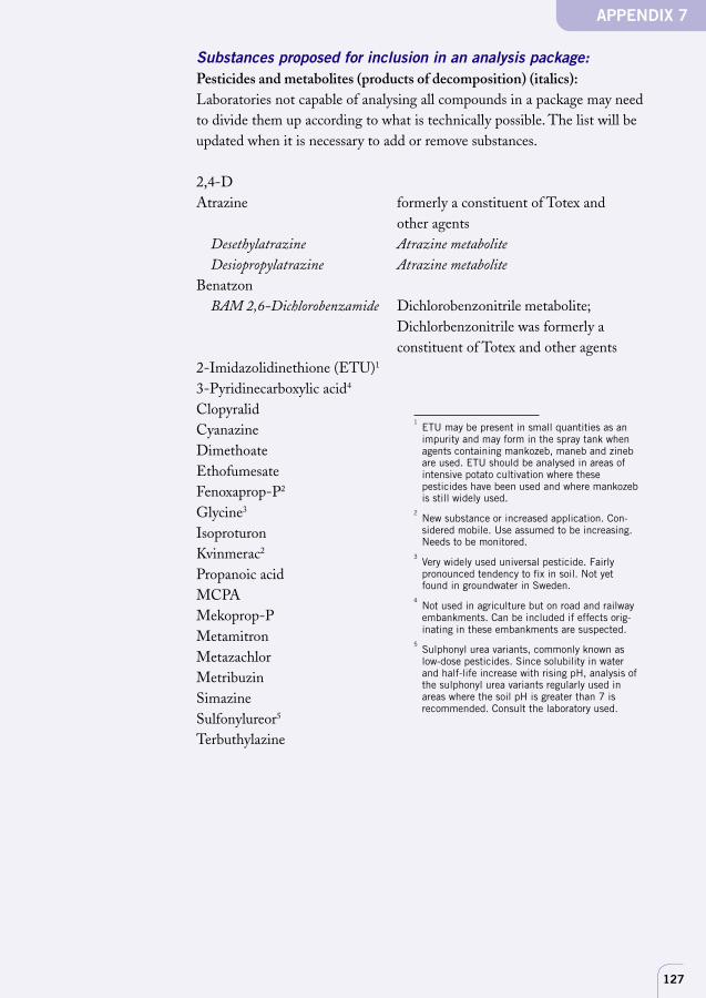
127

Substances proposed for inclusion in an analysis package:Pesticides and metabolites (products of decomposition) (italics):Laboratories not capable of analysing all compounds in a package may needto divide them up according to what is technically possible. The list will beupdated when it is necessary to add or remove substances.

2,4-DAtrazine formerly a constituent of Totex and

other agentsDesethylatrazine Atrazine metaboliteDesiopropylatrazine Atrazine metabolite

BenatzonBAM 2,6-Dichlorobenzamide Dichlorobenzonitrile metabolite;

Dichlorbenzonitrile was formerly aconstituent of Totex and other agents

2-Imidazolidinethione (ETU)1

3-Pyridinecarboxylic acid4

ClopyralidCyanazineDimethoateEthofumesateFenoxaprop-P2

Glycine3

IsoproturonKvinmerac2

Propanoic acidMCPAMekoprop-PMetamitronMetazachlorMetribuzinSimazineSulfonylureor5

Terbuthylazine

APPENDIX 7

1ETU may be present in small quantities as animpurity and may form in the spray tank whenagents containing mankozeb, maneb and zinebare used. ETU should be analysed in areas ofintensive potato cultivation where thesepesticides have been used and where mankozebis still widely used.

2New substance or increased application. Con-sidered mobile. Use assumed to be increasing.Needs to be monitored.

3Very widely used universal pesticide. Fairlypronounced tendency to fix in soil. Not yetfound in groundwater in Sweden.

4Not used in agriculture but on road and railwayembankments. Can be included if effects orig-inating in these embankments are suspected.

5Sulphonyl urea variants, commonly known aslow-dose pesticides. Since solubility in waterand half-life increase with rising pH, analysis ofthe sulphonyl urea variants regularly used inareas where the soil pH is greater than 7 isrecommended. Consult the laboratory used.

128

Water table

A description is given below of how to perform an analysis of a time series

for water table variation at a location. This variation can then be compared

with a reasonably long reference series from a location in a similar geologi-

cal environment.

As mentioned earlier, the approach outlined in the water table chapter isonly suitable in certain clearly defined situations. A time series for fluctua-tions in the water table at the location in question before and after anthro-pogenic disturbance is normally required in order to determine whetherthe water table has in fact been affected by anthropogenic factors. Themonitoring series should begin at least six months prior to the disturbanceand continue for the same length of time afterwards. Readings should betaken at least every 14 days.

This monitoring series can then be compared with a reasonably longreference series from a location in an area of similar geology and climate.These series can often be obtained from the Swedish Geological Survey.

The two series can then be analysed using various methods, eg,• Plotting of the two figures on the same graph (water table against ob-

servation period). Since the two locations have similar geology andclimate, there should be fairly close co-variation between them undernatural unaffected conditions. If the co-variation is replaced by achanged pattern for the local water table simultaneously with theoccurrence of human disturbance, this indicates that the disturbanceis the cause of the change.

• Specific methods for studying water table changes have been develop-ed, e.g., at Chalmers University of Technology, Gothenburg. Amongothers, Chester Svensson (Svensson 1984, Svensson & Sällfors 1985)has developed a method that makes it possible to forecast the highestor lowest groundwater level at a given point. A fairly short series ofmonitoring data (at least three months) from the observation site isneeded. This is compared with a relatively long reference time series.An observation which is below the estimated minimum figure or abovethe estimated maximum figure after the disturbance may then be con-sidered to have an anthropogenic cause.

• Other statistical methods can be used to determine whether two timeseries co-vary or not. One of these is the “double-mass method”(Svensson 1988), which is based on plotting progressively accumulated

APPENDIX 8

129

data from one monitoring series against corresponding data from an-other. The result is a line with a certain gradient. If an event occurswhich affects one of the data series, the gradient on the graph willchange.

• Another method that may be used is to study the co-variation in theform of the correlation coefficient before and after a disturbance in thesurroundings suspected of affecting the water table.

• In some cases, water table fluctuations can also be simulated usingclimatological data and one of the existing hydraulic models, eg, theHBV or SOIL model. However, this presupposes that the models canfirst be calibrated against an unaffected time series that is long enoughto reflect normal fluctuations in climate.

A common feature of the above methods is that they should be applied byspecialists in the field. User-friendly computer software has been develop-ed in recent years. Whether or not these methods can be used depends onthe availability of a fairly short series of monitoring data from the site inquestion, both before and after the disturbance, and also a reasonably longseries of reference data (preferably more than 10 years) from a similargroundwater environment and climatological region.

ReferencesOlofsson, B. (1991): Effects on groundwater by tunnelling in hard crystalline

rocks – analysis of groundwater level data from the Bolmen tunnel, S. Sweden,

1969–1987. – Report from the Department of Soil and Water Resources, Royal

Institute of Technology, TRITA KUT 91:1062.

Svensson, C. (1984): Analys och användning av grundvattennivåobservationer

(”Analysis and use of groundwater level observations”). – Diss. Chalmers Univer-

sity of Technology, Department of Geology, Publ A49. Gothenburg, 126–131.

Svensson, C. & Sällfors, G. (1985): Beräkning av dimensionerande grundvatten-

tryck. 1. Göteborgsregionen (”Modelling size-determinant groundwater pressure.

1. Gothenburg region”). – Chalmers University of Technology, Geohydrological

research group, Notice 78. Gothenburg.

Svensson, C. (1988): Analysis av påverkade grundvattennivåer (”Analysis of affec-

ted ground water levels”). – Chalmers University of Technology, Geohydrological

research group, Notice 84. Gothenburg.

APPENDIX 8

130

Fluoride and radon

FluorideVariation in fluoride concentrations is almost entirely due to natural fac-tors. The highest concentrations are found in some wells bored in igneousand metamorphic rock and sandstone. Examples of this kind of environ-ment are water with long retention times in bedrock comprising younggranites and pegmatites. Concentrations in wells bored in soil are generallylow. Anthropogenic impact is found in only a very few places. Examplesare found in the vicinity of smelting works, where fluorspar or mineralscontaining fluoride have been used and at glassworks. The Drinking WaterRegulations issued by the National Food Administration (SLV FS1993:35) classify water with a fluoride concentration above 6 mg F/l asunfit for consumption, since it poses a risk of bone damage (osteofluor-osis). This water should not be used for drinking purposes or in connectionwith foodstuffs. A limit value for health purposes for water from publicand private sources has been set at 1.3 mg/l, since higher levels may causestains on the teeth of young children (dental fluorosis).

RadonRadon occurs naturally in groundwater, mainly in that from wells bored inrock in areas of uranium-rich bedrock. Examples are uranium-rich sye-nites, vulcanites and pegmatites. Water with a radon concentration exceed-ing 1,000 Bq/l is classified as unfit for consumption in the statutes of theNational Food Administration (SLV FS 1997:32). This water should notbe used for drinking purposes or in connection with foodstuffs. A limitvalue for health purposes for water from public and private sources hasbeen set at 100 Bq/l, since higher levels may pose a threat to the healthof young children.

APPENDIX 9

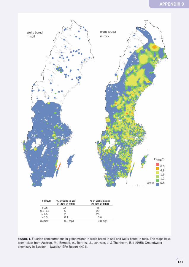
131

APPENDIX 9

F (mg/l) % of wells in soil % of wells in rock(1,322 in total) (9,225 in total)

< 0.8 92.0 46.00.8–1.6 6.0 29.0> 1.6 2.0 25.0> 6.0 0.1 0.6

median 0.2 mg/l 0.8 mg/l

FIGURE 1. Fluoride concentrations in groundwater in wells bored in soil and wells bored in rock. The maps havebeen taken from Aastrup, M., Berntell, A., Bertills, U., Johnson, J. & Thunholm, B. (1995): Groundwaterchemistry in Sweden – Swedish EPA Report 4416.

Wells boredin soil

Wells boredin rock

F (mg/l)

6.0

4.9

1.6

1.2

0.80 200 km

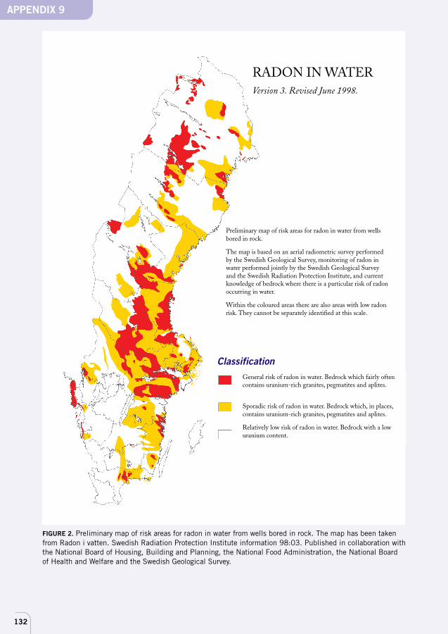
132

APPENDIX 9

FIGURE 2. Preliminary map of risk areas for radon in water from wells bored in rock. The map has been takenfrom Radon i vatten. Swedish Radiation Protection Institute information 98:03. Published in collaboration withthe National Board of Housing, Building and Planning, the National Food Administration, the National Boardof Health and Welfare and the Swedish Geological Survey.

RADON I VATTEN

Prelimin r kartskiss ver riskomr den f r radoni vatten fr n bergborrade brunnar.

Kartan bygger p flygradiometriska m tningarutf rda av SGU, m tningar av radon i vattenutf rda i samarbete mellan SGU och SSI samt kunskapom berggrund med s rskild risk f r radon i vatten.

Inom de markerade riskomr dena finns ven omr denmed l g risk f r radon. Dessa kan ej urskiljas idenna skala.

Mer allm n risk f r radon i vatten.Berggrund i vilken det r relativt vanligtmed uranrika graniter, pegmatiter och apliter.

Mer sporadisk risk f r radon i vatten.Berggrund i vilken det h r och var finnsuranrika graniter, pegmatiter och apliter.

Relativt l g risk f r radon i vatten.Berggrund som har l g uranhalt.

RADON IN WATERVersion 3. Revised June 1998.

Preliminary map of risk areas for radon in water from wellsbored in rock.

The map is based on an aerial radiometric survey performedby the Swedish Geological Survey, monitoring of radon inwater performed jointly by the Swedish Geological Surveyand the Swedish Radiation Protection Institute, and currentknowledge of bedrock where there is a particular risk of radonoccurring in water.

Within the coloured areas there are also areas with low radonrisk. They cannot be separately identified at this scale.

General risk of radon in water. Bedrock which fairly oftencontains uranium-rich granites, pegmatites and aplites.

Sporadic risk of radon in water. Bedrock which, in places,contains uranium-rich granites, pegmatites and aplites.

Relatively low risk of radon in water. Bedrock with a lowuranium content.

Classification

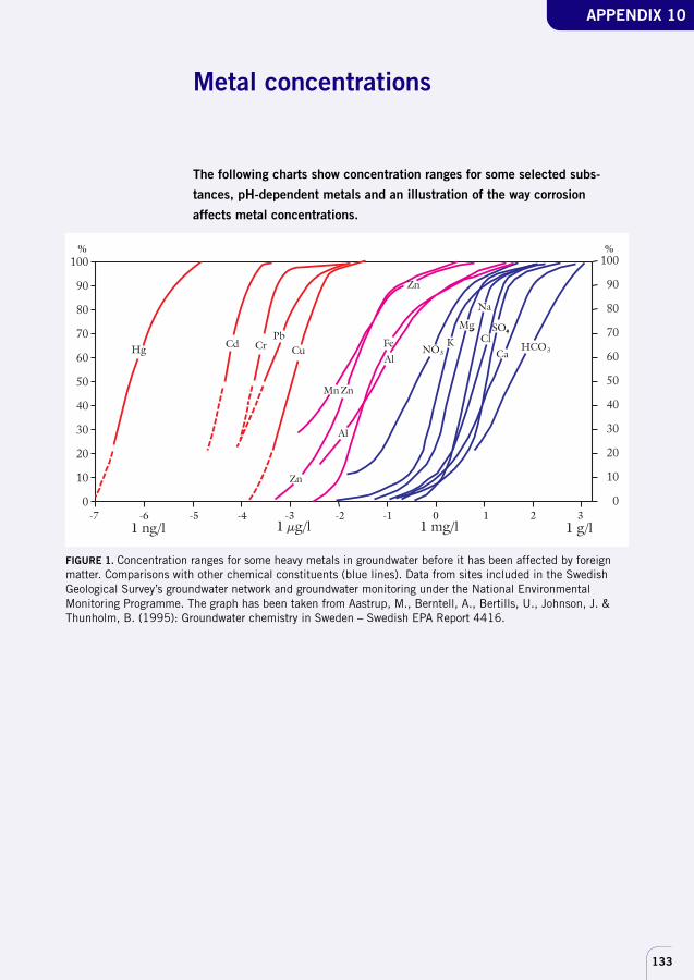
133

Metal concentrations

100

90

80

70

60

50

40

30

20

10

0

100

90

80

70

60

50

40

30

20

10

0

FIGURE 1. Concentration ranges for some heavy metals in groundwater before it has been affected by foreignmatter. Comparisons with other chemical constituents (blue lines). Data from sites included in the SwedishGeological Survey’s groundwater network and groundwater monitoring under the National EnvironmentalMonitoring Programme. The graph has been taken from Aastrup, M., Berntell, A., Bertills, U., Johnson, J. &Thunholm, B. (1995): Groundwater chemistry in Sweden – Swedish EPA Report 4416.

The following charts show concentration ranges for some selected subs-

tances, pH-dependent metals and an illustration of the way corrosion

affects metal concentrations.

APPENDIX 10

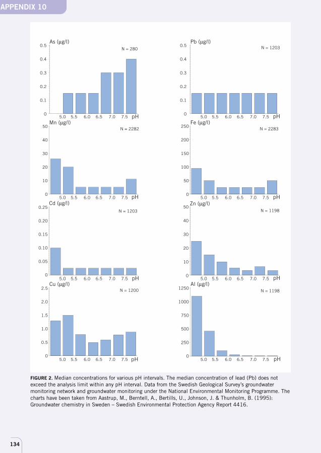
134

As (µg/l) Pb (µg/l)

Mn (µg/l) Fe (µg/l)N = 2283N = 2282

N = 280 N = 1203

5.0 5.5 6.0 6.5 7.0 7.5 5.0 5.5 6.0 6.5 7.0 7.5

5.0 5.5 6.0 6.5 7.0 7.5 5.0 5.5 6.0 6.5 7.0 7.5

5.0 5.5 6.0 6.5 7.0 7.5 5.0 5.5 6.0 6.5 7.0 7.5

5.0 5.5 6.0 6.5 7.0 7.5 5.0 5.5 6.0 6.5 7.0 7.5

0.5

0.4

0.3

0.2

0.1

0

0.5

0.4

0.3

0.2

0.1

0

50

40

30

20

10

0

0.25

0.20

0.15

0.10

0.05

0

2.5

2.0

1.5

1.0

0.5

0

250

200

150

100

50

0

50

40

30

20

10

0

1250

1000

750

500

250

0

Cd (µg/l) Zn (µg/l)

Cu (µg/l) Al (µg/l)

N = 1203

N = 1200 N = 1198

N = 1198

pH pH

pH

pH

pH pH

pH

pH

APPENDIX 10

FIGURE 2. Median concentrations for various pH intervals. The median concentration of lead (Pb) does notexceed the analysis limit within any pH interval. Data from the Swedish Geological Survey’s groundwatermonitoring network and groundwater monitoring under the National Environmental Monitoring Programme. Thecharts have been taken from Aastrup, M., Berntell, A., Bertills, U., Johnson, J. & Thunholm, B. (1995):Groundwater chemistry in Sweden – Swedish Environmental Protection Agency Report 4416.

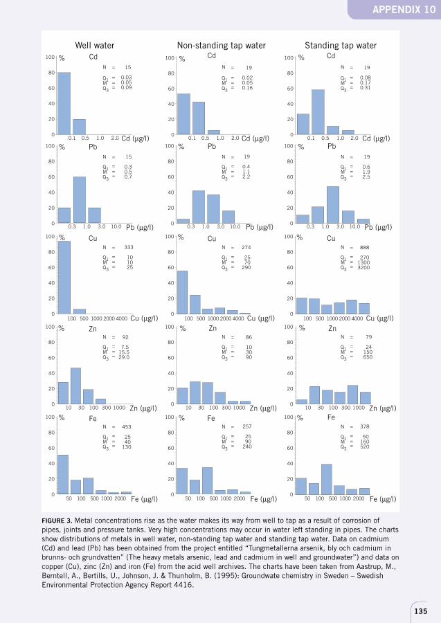
135

FIGURE 3. Metal concentrations rise as the water makes its way from well to tap as a result of corrosion ofpipes, joints and pressure tanks. Very high concentrations may occur in water left standing in pipes. The chartsshow distributions of metals in well water, non-standing tap water and standing tap water. Data on cadmium(Cd) and lead (Pb) has been obtained from the project entitled “Tungmetallerna arsenik, bly och cadmium inbrunns- och grundvatten” (The heavy metals arsenic, lead and cadmium in well and groundwater”) and data oncopper (Cu), zinc (Zn) and iron (Fe) from the acid well archives. The charts have been taken from Aastrup, M.,Berntell, A., Bertills, U., Johnson, J. & Thunholm, B. (1995): Groundwate chemistry in Sweden – SwedishEnvironmental Protection Agency Report 4416.

APPENDIX 10

Cd

Cd (µg/l)

Cd Cd

Pb

Pb (µg/l) Pb (µg/l) Pb (µg/l)

Pb Pb

Cu

Cu (µg/l)

Cu Cu

Fe

Fe (µg/l)

Fe Fe

N =

Q1==M

Q3=

N =

Q1==M

Q3=

N =

Q1==M

Q3=

N =

Q1==M

Q3=

N =

Q1==M

Q3=

N =

Q1==M

Q3=

N =

Q1==M

Q3=

N =

Q1==M

Q3=

N =

Q1==M

Q3=

N =

Q1==M

Q3=

N =

Q1==M

Q3=

N =

Q1==M

Q3=

N =

Q1==M

Q3=

N =

Q1==M

Q3=

N =

Q1==M

Q3=

453

2540

130

257

2590

240

378

50160520

333

101025

15

0.30.50.7

19

0.41.12.2

15

0.030.050.09

19

0.020.050.16

19

0.080.170.31

19

0.61.92.5

274

2570

290

888

27013003200

100 500 1000 2000 4000Cu (µg/l)100 500 1000 2000 4000Cu (µg/l)100 500 1000 2000 4000

50 100 500 1000 2000Fe (µg/l)50 100 500 1000 2000Fe (µg/l)50 100 500 1000 2000

100

80

60

40

20

0

100

80

60

40

20

0

100

80

60

40

20

0

100

80

60

40

20

0

100

80

60

40

20

0

100

80

60

40

20

0

100

80

60

40

20

0

100

80

60

40

20

0

100

80

60

40

20

0

100

80

60

40

20

0

100

80

60

40

20

0

100

80

60

40

20

0

100

80

60

40

20

0

100

80

60

40

20

0

100

80

60

40

20

00.1 0.5 1.0 2.0 Cd (µg/l)0.1 0.5 1.0 2.0 Cd (µg/l)0.1 0.5 1.0 2.0

0.3 1.0 3.0 10.0 0.3 1.0 3.0 10.00.3 1.0 3.0 10.0

%

%

% %

%

%

% %%

% %

% %

% %

Zn

Zn (µg/l)

Zn Zn92

7.515.529.0

86

103090

79

24150650

10 30 100 300 1000Zn (µg/l)10 30 100 300 1000Zn (µg/l)10 30 100 300 1000

Well water Non-standing tap water Standing tap water

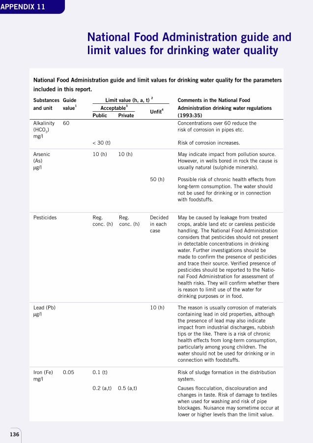
136

APPENDIX 11

National Food Administration guide andlimit values for drinking water quality

National Food Administration guide and limit values for drinking water quality for the parameters

included in this report.

Substances Guide Limit value (h, a, t) 2 Comments in the National Foodand unit value1 Acceptable3 Administration drinking water regulations

Public PrivateUnfit4

(1993:35)Alkalinity 60 Concentrations over 60 reduce the(HCO3) risk of corrosion in pipes etc.mg/l

< 30 (t) Risk of corrosion increases.

Arsenic 10 (h) 10 (h) May indicate impact from pollution source.(As) However, in wells bored in rock the cause isµg/l usually natural (sulphide minerals).

50 (h) Possible risk of chronic health effects fromlong-term consumption. The water shouldnot be used for drinking or in connectionwith foodstuffs.

Pesticides Reg. Reg. Decided May be caused by leakage from treatedconc. (h) conc. (h) in each crops, arable land etc or careless pesticide

case handling. The National Food Administrationconsiders that pesticides should not presentin detectable concentrations in drinkingwater. Further investigations should bemade to confirm the presence of pesticidesand trace their source. Verified presence ofpesticides should be reported to the Natio-nal Food Administration for assessment ofhealth risks. They will confirm whether thereis reason to limit use of the water fordrinking purposes or in food.

Lead (Pb) 10 (h) The reason is usually corrosion of materialsµg/l containing lead in old properties, although

the presence of lead may also indicateimpact from industrial discharges, rubbishtips or the like. There is a risk of chronichealth effects from long-term consumption,particularly among young children. Thewater should not be used for drinking or inconnection with foodstuffs.

Iron (Fe) 0.05 0.1 (t) Risk of sludge formation in the distributionmg/l system.

0.2 (a,t) 0.5 (a,t) Causes flocculation, discolouration andchanges in taste. Risk of damage to textileswhen used for washing and risk of pipeblockages. Nuisance may sometime occur atlower or higher levels than the limit value.

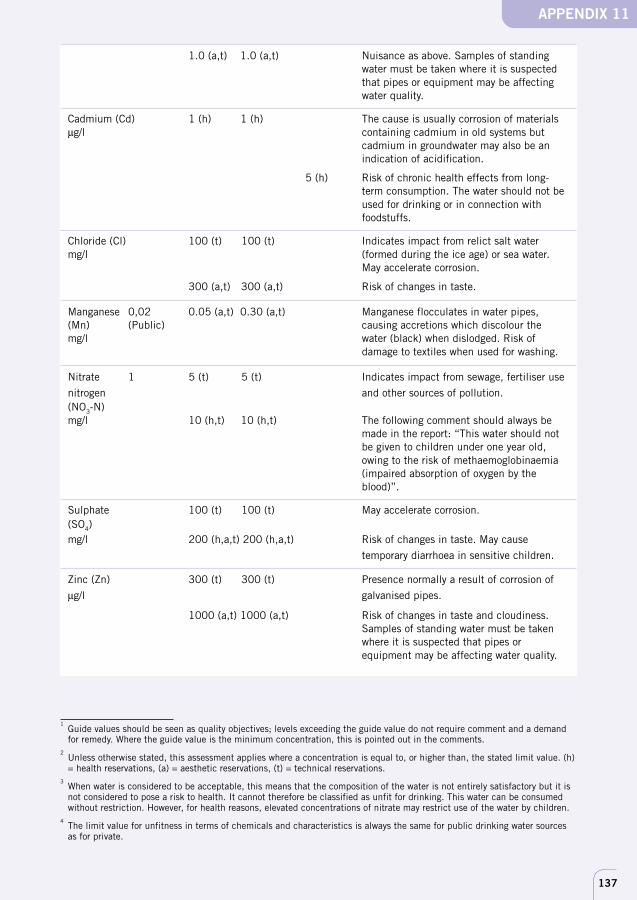
137

1.0 (a,t) 1.0 (a,t) Nuisance as above. Samples of standingwater must be taken where it is suspectedthat pipes or equipment may be affectingwater quality.

Cadmium (Cd) 1 (h) 1 (h) The cause is usually corrosion of materialsµg/l containing cadmium in old systems but

cadmium in groundwater may also be anindication of acidification.

5 (h) Risk of chronic health effects from long-term consumption. The water should not beused for drinking or in connection withfoodstuffs.

Chloride (Cl) 100 (t) 100 (t) Indicates impact from relict salt watermg/l (formed during the ice age) or sea water.

May accelerate corrosion.

300 (a,t) 300 (a,t) Risk of changes in taste.

Manganese 0,02 0.05 (a,t) 0.30 (a,t) Manganese flocculates in water pipes,(Mn) (Public) causing accretions which discolour themg/l water (black) when dislodged. Risk of

damage to textiles when used for washing.

Nitrate 1 5 (t) 5 (t) Indicates impact from sewage, fertiliser use

nitrogen and other sources of pollution.(NO3-N)mg/l 10 (h,t) 10 (h,t) The following comment should always be

made in the report: “This water should notbe given to children under one year old,owing to the risk of methaemoglobinaemia(impaired absorption of oxygen by theblood)”.

Sulphate 100 (t) 100 (t) May accelerate corrosion.(SO4)mg/l 200 (h,a,t) 200 (h,a,t) Risk of changes in taste. May cause

temporary diarrhoea in sensitive children.

Zinc (Zn) 300 (t) 300 (t) Presence normally a result of corrosion of

µg/l galvanised pipes.

1000 (a,t) 1000 (a,t) Risk of changes in taste and cloudiness.Samples of standing water must be takenwhere it is suspected that pipes orequipment may be affecting water quality.

APPENDIX 11

1Guide values should be seen as quality objectives; levels exceeding the guide value do not require comment and a demandfor remedy. Where the guide value is the minimum concentration, this is pointed out in the comments.

2Unless otherwise stated, this assessment applies where a concentration is equal to, or higher than, the stated limit value. (h)= health reservations, (a) = aesthetic reservations, (t) = technical reservations.

3When water is considered to be acceptable, this means that the composition of the water is not entirely satisfactory but it isnot considered to pose a risk to health. It cannot therefore be classified as unfit for drinking. This water can be consumedwithout restriction. However, for health reasons, elevated concentrations of nitrate may restrict use of the water by children.

4The limit value for unfitness in terms of chemicals and characteristics is always the same for public drinking water sourcesas for private.

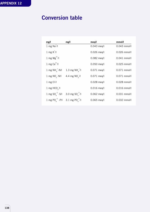
138

APPENDIX 12

Conversion table

mg/l mg/l meq/l mmol/l

1 mg Na+/l 0.043 meq/l 0.043 mmol/l

1 mg K+/l 0.026 meq/l 0.026 mmol/l

1 mg Mg2+

/l 0.082 meq/l 0.041 mmol/l

1 mg Ca2+

/l 0.050 meq/l 0.025 mmol/l

1 mg NH4

+-N/l 1.3 mg NH

4

+/l 0.071 meq/l 0.071 mmol/l

1 mg NO3

--N/l 4.4 mg NO

3

-/l 0.071 meq/l 0.071 mmol/l

1 mg Cl-/l 0.028 meq/l 0.028 mmol/l

1 mg HCO3

-/l 0.016 meq/l 0.016 mmol/l

1 mg SO4

2- -S/l 3.0 mg SO

4

2-/l 0.062 meq/l 0.031 mmol/l

1 mg PO4

2- -P/l 3.1 mg PO

4

2-/l 0.065 meq/l 0.032 mmol/l

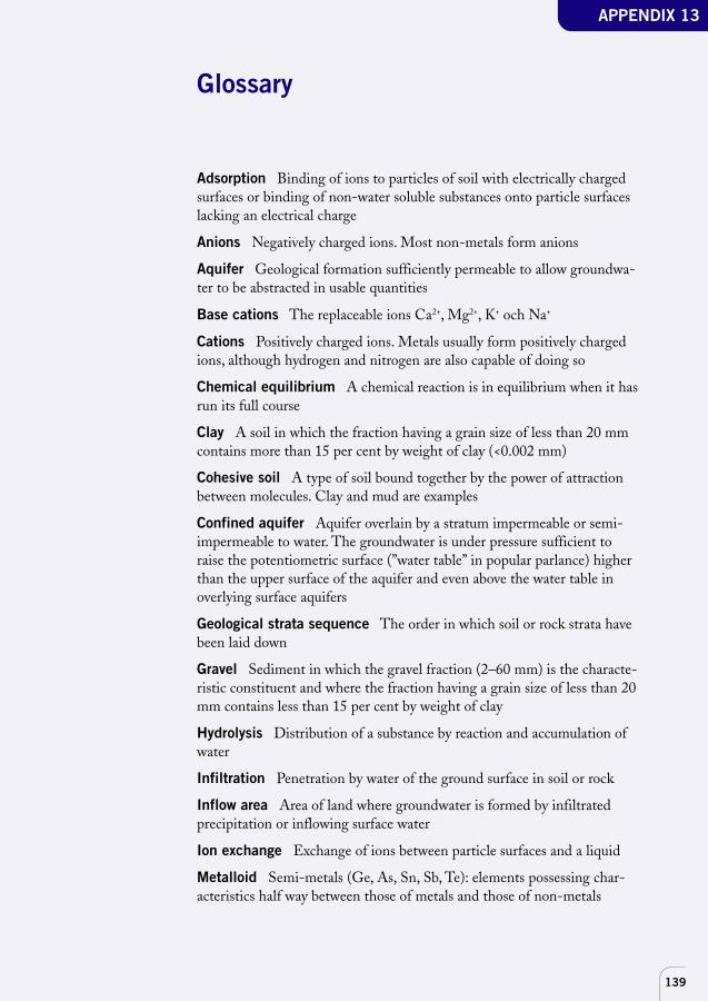
139

Glossary

Adsorption Binding of ions to particles of soil with electrically chargedsurfaces or binding of non-water soluble substances onto particle surfaceslacking an electrical charge

Anions Negatively charged ions. Most non-metals form anions

Aquifer Geological formation sufficiently permeable to allow groundwa-ter to be abstracted in usable quantities

Base cations The replaceable ions Ca2+, Mg2+, K+ och Na+

Cations Positively charged ions. Metals usually form positively chargedions, although hydrogen and nitrogen are also capable of doing so

Chemical equilibrium A chemical reaction is in equilibrium when it hasrun its full course

Clay A soil in which the fraction having a grain size of less than 20 mmcontains more than 15 per cent by weight of clay (<0.002 mm)

Cohesive soil A type of soil bound together by the power of attractionbetween molecules. Clay and mud are examples

Confined aquifer Aquifer overlain by a stratum impermeable or semi-impermeable to water. The groundwater is under pressure sufficient toraise the potentiometric surface (”water table” in popular parlance) higherthan the upper surface of the aquifer and even above the water table inoverlying surface aquifers

Geological strata sequence The order in which soil or rock strata havebeen laid down

Gravel Sediment in which the gravel fraction (2–60 mm) is the characte-ristic constituent and where the fraction having a grain size of less than 20mm contains less than 15 per cent by weight of clay

Hydrolysis Distribution of a substance by reaction and accumulation ofwater

Infiltration Penetration by water of the ground surface in soil or rock

Inflow area Area of land where groundwater is formed by infiltratedprecipitation or inflowing surface water

Ion exchange Exchange of ions between particle surfaces and a liquid

Metalloid Semi-metals (Ge, As, Sn, Sb, Te): elements possessing char-acteristics half way between those of metals and those of non-metals

APPENDIX 13

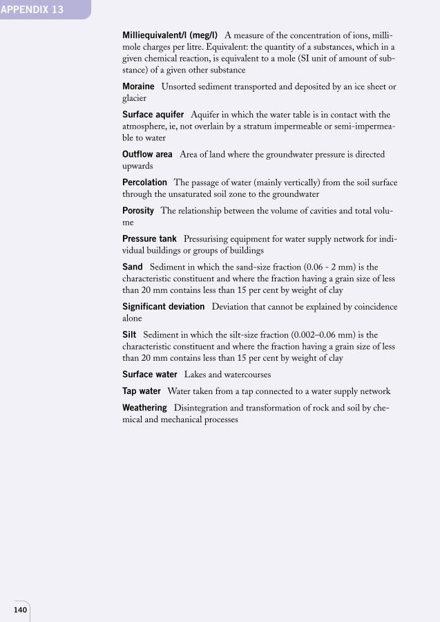
140

APPENDIX 13

Milliequivalent/l (meg/l) A measure of the concentration of ions, milli-mole charges per litre. Equivalent: the quantity of a substances, which in agiven chemical reaction, is equivalent to a mole (SI unit of amount of sub-stance) of a given other substance

Moraine Unsorted sediment transported and deposited by an ice sheet orglacier

Surface aquifer Aquifer in which the water table is in contact with theatmosphere, ie, not overlain by a stratum impermeable or semi-impermea-ble to water

Outflow area Area of land where the groundwater pressure is directedupwards

Percolation The passage of water (mainly vertically) from the soil surfacethrough the unsaturated soil zone to the groundwater

Porosity The relationship between the volume of cavities and total volu-me

Pressure tank Pressurising equipment for water supply network for indi-vidual buildings or groups of buildings

Sand Sediment in which the sand-size fraction (0.06 - 2 mm) is thecharacteristic constituent and where the fraction having a grain size of lessthan 20 mm contains less than 15 per cent by weight of clay

Significant deviation Deviation that cannot be explained by coincidencealone

Silt Sediment in which the silt-size fraction (0.002–0.06 mm) is thecharacteristic constituent and where the fraction having a grain size of lessthan 20 mm contains less than 15 per cent by weight of clay

Surface water Lakes and watercourses

Tap water Water taken from a tap connected to a water supply network

Weathering Disintegration and transformation of rock and soil by che-mical and mechanical processes

---

-

G R O U N D W A T E R I S N O T as well protected as one mightimagine. It is affected by pollutants in the ground, byacidification and eutrophication. A rise or fall in the water tablecan cause harmful effects. Groundwater quality can beinterpreted and evaluated using the model criteria in this report.

The report is one of a series of six reports published by theSwedish Environmental Protection Agency under the headingE N V I R O N M E N TA L Q U A L I T Y C R I T E R I A . The reports areintended to be used by local and regional authorities, as well asother agencies, but also contain useful information for anyonewith responsibility for, and an interest in, good environmentalquality.

Reports available in English are:Report No.

• Lakes and Watercourses 5050• Coasts and Seas 5052• Contaminated Sites 5053

Abridged versions in English of all the six reports are availableon the Agency’s home page: www.environ.se (under the headlinelegislation/guidelines).

REPORT 5051

Groundwater

REPORT 5051


Groundwater

Environm

ental Quality C

riteria - Groundw

aterR

EP

OR

T 50

51

Documents

· mental effects, etc. This report is one of six in a series which purpose is to fill that infor-mation gap, by enabling counties and municipalities to make compara-