Embed Size (px)
Citation preview

Brigham Young UniversityBYU ScholarsArchive
All Theses and Dissertations
2018-04-01
Effects of Acid Whey Marination on Tenderness,Sensory and Other Quality Parameters of Beef Eyeof RoundJason KimBrigham Young University
Follow this and additional works at: https://scholarsarchive.byu.edu/etd
Part of the Nutrition Commons
This Thesis is brought to you for free and open access by BYU ScholarsArchive. It has been accepted for inclusion in All Theses and Dissertations by anauthorized administrator of BYU ScholarsArchive. For more information, please contact [email protected], [email protected].
BYU ScholarsArchive CitationKim, Jason, "Effects of Acid Whey Marination on Tenderness, Sensory and Other Quality Parameters of Beef Eye of Round" (2018).All Theses and Dissertations. 6758.https://scholarsarchive.byu.edu/etd/6758

Effects of Acid Whey Marination on Tenderness, Sensory
and Other Quality Parameters of Beef Eye of Round
Jason Kim
A thesis submitted to the faculty of Brigham Young University
in partial fulfillment of the requirements for the degree of
Master of Science
Michael L. Dunn, Chair Frost M. Steele
Laura K. Jefferies
Department of Nutrition, Dietetics, and Food Science
Brigham Young University
Copyright © 2018 Jason Kim
All Rights Reserved
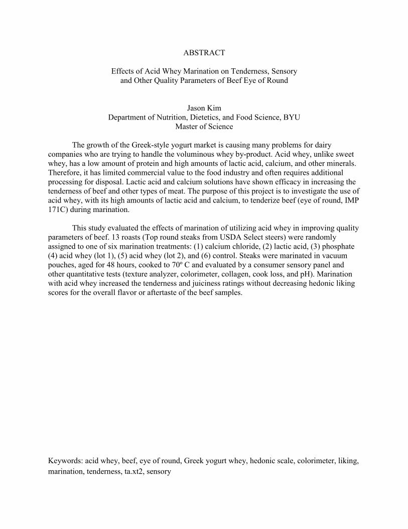
ABSTRACT
Effects of Acid Whey Marination on Tenderness, Sensory and Other Quality Parameters of Beef Eye of Round
Jason Kim Department of Nutrition, Dietetics, and Food Science, BYU
Master of Science
The growth of the Greek-style yogurt market is causing many problems for dairy companies who are trying to handle the voluminous whey by-product. Acid whey, unlike sweet whey, has a low amount of protein and high amounts of lactic acid, calcium, and other minerals. Therefore, it has limited commercial value to the food industry and often requires additional processing for disposal. Lactic acid and calcium solutions have shown efficacy in increasing the tenderness of beef and other types of meat. The purpose of this project is to investigate the use of acid whey, with its high amounts of lactic acid and calcium, to tenderize beef (eye of round, IMP 171C) during marination.
This study evaluated the effects of marination of utilizing acid whey in improving quality
parameters of beef. 13 roasts (Top round steaks from USDA Select steers) were randomly assigned to one of six marination treatments: (1) calcium chloride, (2) lactic acid, (3) phosphate (4) acid whey (lot 1), (5) acid whey (lot 2), and (6) control. Steaks were marinated in vacuum pouches, aged for 48 hours, cooked to 70º C and evaluated by a consumer sensory panel and other quantitative tests (texture analyzer, colorimeter, collagen, cook loss, and pH). Marination with acid whey increased the tenderness and juiciness ratings without decreasing hedonic liking scores for the overall flavor or aftertaste of the beef samples. Keywords: acid whey, beef, eye of round, Greek yogurt whey, hedonic scale, colorimeter, liking, marination, tenderness, ta.xt2, sensory

ACKNOWLEDGMENTS
I would like to express my gratitude to the faculty and staff of the department of
Nutrition, Dietetics, and Food Science for their time in teaching and mentoring me throughout
my undergraduate and graduate degrees at BYU. I am grateful to Dr. Steele, Dr. Jefferies and Dr.
Dunn for their help on my committee, and Dr. Dunn for serving as my committee chair. I could
not have produced as fine of research without their expert guidance along the way. Thanks are
also in order for the students of the food research lab and my fellow graduate students who
helped me think through many problems.

iv
TABLE OF CONTENTS
TITLE PAGE ................................................................................................................................... i
ABSTRACT .................................................................................................................................... ii
ACKNOWLEDGMENTS ............................................................................................................. iii
TABLE OF CONTENTS ............................................................................................................... iv
LIST OF TABLES ......................................................................................................................... vi
LIST OF FIGURES ...................................................................................................................... vii
INTRODUCTION .......................................................................................................................... 1
Summary ..................................................................................................................................... 1
Acid Whey .................................................................................................................................. 2
Meat Tenderization ..................................................................................................................... 3
Objectives ................................................................................................................................... 5
Materials and Methods .................................................................................................................... 5
Product Selection ........................................................................................................................ 5
Treatments................................................................................................................................... 5
Packaging and Marination .......................................................................................................... 6
Cooking ....................................................................................................................................... 7
pH ................................................................................................................................................ 7
Cook Loss ................................................................................................................................... 7
Color ........................................................................................................................................... 7
Shear Force ................................................................................................................................. 8
Scanning Electron Microscopy ................................................................................................... 8

v
Collagen Content ........................................................................................................................ 9
Consumer Panel Analysis ........................................................................................................... 9
Statistical Analysis .................................................................................................................... 11
RESULTS AND DISCUSSION ................................................................................................... 11
Compositional Analysis ............................................................................................................ 11
Consumer Sensory Evaluation .................................................................................................. 11
Compositional and Textural Properties .................................................................................... 12
Color ......................................................................................................................................... 15
Electron Microscopy ................................................................................................................. 16
Conclusion ................................................................................................................................ 19
Complete References .................................................................................................................... 20
Appendix ....................................................................................................................................... 25
Texture Analyzer Test Settings ................................................................................................. 25
Collagen Method - Detailed ...................................................................................................... 25
Table 5 Complete Proximate Composition (%) and Mineral Content (ppm) of Acid Wheys .. 27
Table 6 Complete Mineral Analysis (ppm) .............................................................................. 27
Statistical Output ....................................................................................................................... 28
Sensory Comments ................................................................................................................... 84

vi
LIST OF TABLES
Table 1 Proximate composition (%) and mineral content (ppm) of acid whey ............................ 11
Table 2 Consumer acceptance and hedonic ratings for beef eye of round steaks marinated in
different solutions ......................................................................................................................... 12
Table 3 Means for soluble collagen, insoluble collagen, cook loss percentage, pH, and shear
force .............................................................................................................................................. 13
Table 4 Effect of acid whey and other marinade treatments on color of beef eye of round. ........ 15
Table 5 Proximate Composition (%) and Mineral Content (ppm) of Acid Whey ........................ 27
Table 6 Mineral Analysis (ppm) ................................................................................................... 27

vii
LIST OF FIGURES
Figure 1 Scanning electron micrograph (SEM) of raw beef muscles with different treatments
(control-no treatment, acid whey, calcium chloride, lactic acid, and phosphate) ......................... 18

1
INTRODUCTION
Summary
The expansion of Greek-style yogurt in the U.S. yogurt industry in the past ten years is
one of the most remarkable events in food production and sales in recent history (McCormack
2016). Greek-style yogurt is traditionally made by straining the fermented yogurt curd in a cloth
bag, removing the acid whey until it reaches a desired solids level. In the food industry this step
is achieved by mechanically separating the acid whey from the yogurt using a centrifugal
separator or a filtration membrane (Nsabimana and others 2005). The growth of this market has
caused a lot of problems for dairy companies who are attempting to handle large quantities of
this acid whey byproduct (Uderwerella and others 2017).
Greek-style yogurt acid whey, unlike sweet whey from traditional cheese production, is
low in protein and high in lactic acid, calcium, and other minerals. Ultrafiltration can be used to
recover the protein from this whey. However, the loss of membrane efficiency, or membrane
fouling, is a longstanding problem in facilities that utilize this technology (Berg and others
2014).
Membrane fouling during the processing of acid whey is attributed mainly to the
precipitation of calcium salts, especially calcium phosphates (Hanemaaijer and others 1989). The
high level of process inputs required to recover the low levels of protein in acid whey reduces its
commercial value to the food industry. Many companies in the dairy industry currently sell their
acid whey to farmers as animal feed. In efforts to maximize profits, and facilitate disposal, recent
research has explored new ways to apply or process acid whey for human consumption. Wojciak
and others. (2014), for example, found that use of acid whey in sausages could be used

2
effectively to improve the microbiological quality, and that it could produce a similar color to
sausage treated with a nitrite curing salt.
While the low protein content of acid whey makes it a low-value byproduct, the
abundance of lactic acid and calcium in the whey may lead to alternative uses in the food
industry. Lactic acid and calcium solutions have been found to be effective in increasing the
tenderness in beef and other cuts of meat (Berg and others 2001; Ostoja and Cierach 2003). The
purpose of this research was to investigate the use of acid whey in marinade solutions, as a
means to tenderize beef (eye of round, IMP 171C).
Acid Whey
Whey is the liquid byproduct of cheese and Greek-style yogurt manufacture. The whey
from hard cheeses is referred to as sweet whey, and is relatively high in protein, as well as
containing minerals and some acid. Sweet whey is the principal source of the high-value whey
protein powders that are in high demand worldwide. The whey derived from Greek yogurt
manufacture (or quark or cream cheese production) is referred to as acid whey. It is low in
protein, and contains appreciable amounts of lactose, minerals, and lactic acid. The disposal of
acid whey is a major problem worldwide. Ultrafiltration of both acid whey and sweet whey are
practiced (Ganju and Gogate 2017); however, there are many issues that arise due to membrane
fouling during processing (Berg and others 2014). Pretreatment of whey to remove calcium salts
has been shown to increase membrane productivity (Patel and Merson 1978, Patocka and Jelen
1991), however, these additional process steps reduce production capacities and increase cost.
The low protein yields with acid whey currently make this commercially non-viable.

3
As a result of the difficulty and costs of processing acid whey through filtration, there has
been interest in using whole, liquid acid whey as a functional ingredient in different applications.
Skrypolenk and Jasinska (2015) explored the idea of using acid whey as a base for creating
probiotic beverages. Vajda and others (2013) examined the effect of acid whey concentrate on
thermophysical properties of a milk based ice cream. Sady and others (2013) studied the
application of acid whey in orange drink production.
A limited amount of research has been conducted, looking at acid whey as a process
additive in meat products. Wojciak and others (2014) used acid whey with mustard seed to
replace nitrites in cooked sausages, with positive effects. Stadnik and Stasiak (2016) reported on
the physicochemical properties of pork loin marinated in acid whey prior to dry curing. The acid
whey marination, combined with sea salt, resulted in reduced browning, and was protective
against oxidation. Wojciak and others (2015) explored the use of acid whey as a marinade for
production of fermented beef eye of round. They found that acid whey decreased the pH,
increased the red color value as well as oxidative stability, but did not have appreciable sensory
effects in a limited eight-person trained panel. However, there has not been much research done
to look at the effects of acid whey on the tenderness of beef. The high amounts of acid and
calcium could potentially increase the tenderness.
Meat Tenderization
The sensory characteristics (texture, flavor, aroma, and color) of meat are important
attributes in determining its quality. Tenderness and associated juiciness are among the most
important quality attributes related to meat texture and eating quality. The texture of meat is
predominantly determined by the moisture and fat contents, as well as the types and amounts of
structural proteins (Aktas and Kaya 2001). Collagen is a major structural protein of

4
intramuscular connective tissue that plays an important role in binding the myofibers to provide
structure. (Borg and Caulfield 1980; Chang and others 2010). It has been shown that the
toughness of a muscle is proportional to its intramuscular collagen content (Aktas 2003).
Many methods for altering meat tenderness have been evaluated, including the use of
marinades (Burke and Monahan 2003). Acidic marination involves the immersion of meat in a
solution containing vinegar (Kijowski 1993; Kijowski and Mast 1993), wine or fruit juice
(Arganosa and Marriott 1989; Burke and Monahan 2003), lactic acid (Aktas and Kaya 2001), or
other acidulants. Weak organic acids were tested for their ability to increase meat tenderization
either directly, through the physical weakening of muscle structures due to the swelling of
myofibers (Rao and Gault 1990) and direct weakening of the perimysial connective tissue (Lewis
and others 1991), or indirectly, through the activation of proteolysis by a release of cathepsins
from lysosomes (Berge and others 2001).
Presently, sodium phosphate is commonly used in meat processing, and has been
documented to increase protein solubility and the water-binding ability of meat (Hellendoorn
1962; Trout and Schmidt 1986). Smith and others (1984) concluded that injection of brine
containing sodium tri-polyphosphate into pork longissimus increased juiciness and reduced
Warner Bratzler shear values, and also increased juiciness when injected into beef
semimembranosus. While sodium phosphate is not a component of acid whey, calcium
phosphate (hydroxyapatite) is present at significant levels.
Several studies have evaluated calcium, in the form of calcium chloride, as a means for
increasing beef tenderness (Wheeler and others 1992; Whipple and Koohmaraie, 1993; Kerth
and others 1995). The tenderizing effects of marinating or injecting beef cuts with calcium
chloride, are postulated to relate in part to increased calcium- activated proteolysis (Cao and

5
others 2012; Morgan and others 1991; Behrends and others 2005). However, a 10% injection of
0.3 M calcium chloride has been shown to have an adverse effect on palatability, imparting a
bitter, metallic and sour taste to the cooked product (Eilers and others 1994; Morris and others
1997). Calcium phosphate was shown to have less bitterness than calcium chloride, when applied
to cottage cheese (Puspitasari and others 1991), which suggests that the hydroxyapatite in acid
whey, may not be a significant cause of off-flavor development during marination.
Objectives
The exponential growth of the Greek yogurt industry led to the increase in supply of
Greek yogurt acid whey. This by-product has shown to be very difficult to process for food
consumption due to the low pH and high mineral content. Researchers have looked to explore
methods to improve processing and discovers new applications to use to acid whey. The
objective of this study is to evaluate the use of acid whey as a marinade for beef and its effects
on tenderness and other quality parameters.
Materials and Methods
Product Selection
Eye of round (semitendinosus) roasts (171C IMPS/NAMP) (n=13) were obtained from
grain fed cattle of about 15-18 months from a local beef packing facility. Vacuum packaged eye
of round roasts were transported to Brigham Young University and fabricated into steaks (2.54
cm thick). The steaks were then sub-divided into 3.00 cm x 3.00cm steak cubes prior to
application of treatments.
Treatments
The steak cubes from each roast were assigned randomly to either a control (no
marinade) or one of the five marination-treatments groups: calcium chloride, lactic acid, sodium

6
phosphate, acid whey (lot 1), and acid whey (lot 2). Calcium chloride marinade consisted of a pH
7.03 solution of (4.29 g/L) calcium chloride (Harris & Ford LLC, Indianapolis, IN) in distilled
water. The calcium concentration was designed to match the average calcium concentration of
the two lots of acid whey. Lactic acid marinade was prepared by adding a 50% lactic acid
solution (Purac INC, Blair, Nebraska) to distilled water to a target pH of 4.26. This pH matched
the pH of the acid whey lots collected from Greek yogurt production. The phosphate treatment
contained 2% sodium phosphate (Gusto M31 Sodium Phosphate, Formtech Solutions Inc,
Schenevus, NY) in distilled water, with a final pH of 7.32. This was prepared as instructed by
Formtech Solutions Inc. for use in meat marination. The two lots of acid whey were obtained
from a local Greek yogurt manufacturer, and were produced on different manufacturing days.
The steaks and marinades were combined in vacuum pouches to determine the effect of the
marination.
Packaging and Marination
386 steak cubes were cut from 13 different eye round roasts and those individual steaks
were vacuum packaged with nothing (control) or with the appropriated marination treatment
solution in 20.3 x 30.48cm vacuum bags (nylon/polyethylene) at 23.5º C (Vacmaster VP215).
The 386 steak cubes were evenly distributed among the 6 different treatments (minimum of 60
steak cubes per treatment). All marinades were added to the steak cubes to equal 25% of raw cut
weight (25% wt/wt). Steaks were marinated for 48 hours at 4º C. Following the 48-hour
marination, the samples were removed from the vacuum bag to have the pH and weight recorded
and the remaining liquid in the bag was discarded.

7
Cooking
Steaks were cooked in an electric convection oven at 260º C (Model: JTP18; GE
Appliances) on a broiler pan. Temperature was monitored with a hypodermic temperature probe
coupled with a digital thermocouple thermometer (Fluke 52II Thermometer). As the geometric
center of each steak reached a final temperature of 71º ± 2 C they were removed from the oven
and placed on a cooling rack for 2 min. The steak samples were then vacuum packaged in a 20.3
x 30.48 cm vacuum bag (nylon/polyethylene) at 23.5º C (Vacmaster VP215) and stored at 4º C
until they were analyzed for weight, collagen, color, shear force, scanning electron microscope
and sensory.
pH
An Orion Star pH meter (A211 benchtop model 320) with an Orion 9120APAW
KNIPHE electrode, designed to measure surface pH, was used to test the pH of the meat before
and after each marinade treatment. The probe was calibrated using pH buffer standards before it
was used to determine the final pH. The probe was held on the surface of each cube of meat until
a final pH was recorded.
Cook Loss
Each cube (n=442) of meat was weighed before the marinade treatment, after the
marination, and after cooking. To calculate the percent loss the following formula was used:
{(weight after marination - weight after cooking)/weight after marination} *100.
Color
A model Colorflex EZ Hunter lab colorimeter, equipped with a 25 mm-diameter
measuring area, was used to determine the color change of the uncooked meat due to each
treatment (n = 423). The colorimeter was calibrated using color standard tiles before each day of

8
use. The instrument was set to illuminant A and Commission International de l’Eclariage (CIE)
L* (lightness), a*(redness), and b*(yellowness) values were recorded. To capture a complete
representation of the color, the samples were rotated after each measurement for a total of 5
measurements per sample.
Shear Force
Following cooking and refrigerated storage overnight at 4º C, a cylindrical core sample
was taken from the center of each cube (1.5 cm diameter) by cutting with a cork borer parallel to
the muscle fiber orientation (n= 385). Using a texture analyzer (TAXT2, Texture Technologies,
Hamilton, MA) with a Warner-Bratzler attachment, the core samples were sheared perpendicular
to the muscle fibers using settings suggested by the instrument manufacturer. Compression-mode
setting, with a contact force of 1 g and trigger force of 20 g was used with a test speed of 3.3
mm/sec over a 30-mm distance. After the test was completed the remaining portions of steaks
were refrigerated at 4º C and used later to determine soluble and insoluble collagen.
Scanning Electron Microscopy
Samples of uncooked marinated beef were produced by cutting a small section (<0.5 mm
thick) against the natural grain of the meat samples. The samples were placed in a buffer solution
(2% glutaraldehyde in 0.06 M sodium cacodylate) for 24 h, then rinsed with 0.03M sodium
cacodylate buffer 6 times at 10 min intervals. Rinsed samples were then fixed with 1% osmium
tetroxide (OsO4) for 1 h. Next, the samples were rinsed with distilled water to remove any
remaining OsO4. Subsequent samples were then dehydrated by gradient ethanol series (10, 30,
50, 70, and 95 vol.%) for 15 min in each solution and in absolute ethanol for 45 min. The
samples were then dried in a critical point dryer (Tousimis 931, Rockville, MD), and sputter
coated with gold/palladium (10nm). The specimens were examined and photographed using
9
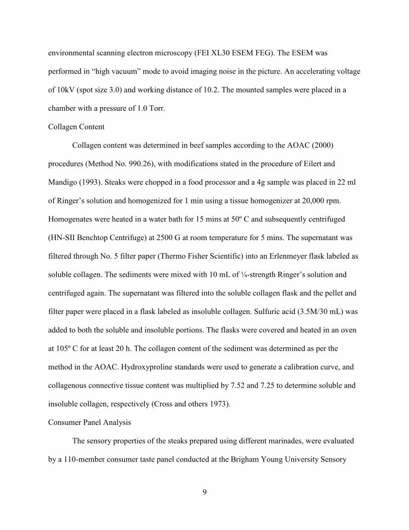
environmental scanning electron microscopy (FEI XL30 ESEM FEG). The ESEM was
performed in “high vacuum” mode to avoid imaging noise in the picture. An accelerating voltage
of 10kV (spot size 3.0) and working distance of 10.2. The mounted samples were placed in a
chamber with a pressure of 1.0 Torr.
Collagen Content
Collagen content was determined in beef samples according to the AOAC (2000)
procedures (Method No. 990.26), with modifications stated in the procedure of Eilert and
Mandigo (1993). Steaks were chopped in a food processor and a 4g sample was placed in 22 ml
of Ringer’s solution and homogenized for 1 min using a tissue homogenizer at 20,000 rpm.
Homogenates were heated in a water bath for 15 mins at 50º C and subsequently centrifuged
(HN-SII Benchtop Centrifuge) at 2500 G at room temperature for 5 mins. The supernatant was
filtered through No. 5 filter paper (Thermo Fisher Scientific) into an Erlenmeyer flask labeled as
soluble collagen. The sediments were mixed with 10 mL of ¼-strength Ringer’s solution and
centrifuged again. The supernatant was filtered into the soluble collagen flask and the pellet and
filter paper were placed in a flask labeled as insoluble collagen. Sulfuric acid (3.5M/30 mL) was
added to both the soluble and insoluble portions. The flasks were covered and heated in an oven
at 105º C for at least 20 h. The collagen content of the sediment was determined as per the
method in the AOAC. Hydroxyproline standards were used to generate a calibration curve, and
collagenous connective tissue content was multiplied by 7.52 and 7.25 to determine soluble and
insoluble collagen, respectively (Cross and others 1973).
Consumer Panel Analysis
The sensory properties of the steaks prepared using different marinades, were evaluated
by a 110-member consumer taste panel conducted at the Brigham Young University Sensory

10
Laboratory. The panel was conducted in a single session in the afternoon. Panelists were
recruited from a database of university employees and students and were selected based on their
willingness to evaluate steak. Both genders were equally represented, with approximately equal
representation among age categories from age 20 to 60 y. The study was approved by the
university Institutional Review Board and panelists provided their informed consent. The steaks
were prepared by cutting each steak into 2.54 cm x 3 cm x 3 cm cubes. Each steak cube was
marinated and cooked as described previously. Cooked samples were placed in an insulated
steam table set at 71º C to keep them warm until serving. Fresh samples were prepared every 30
mins, by cutting each sample with the grain of the meat into four equal pieces, and then each
panelist was given two of the four pieces. The panelists were served five different samples, each
representing a different treatment. Samples were served in 2 oz. plastic cups, labeled with a
random 3-digit blinding code; and panelists were directed to consume the samples in order from
left to right. Sample presentation order was randomized to ensure that each sample saw an
approximately equal number of presentations in each position. Questions were presented one-at-
a-time on a computer screen and data were collected using Compusense® 5 (version 4.6)
software (Compusense Inc., Guelph, Ontario, Canada). Panelists evaluated appearance, aroma,
flavor, texture, and overall liking using a discrete 9-point hedonic scale, where 9 = like
extremely, 5 = neither like nor dislike, and 1=dislike extremely. They also evaluated the cooked
steaks from each treatment for tenderness and juiciness using a 5-point just about right (JAR)
ideality scale (1=definitely not juicy enough, 3=just about right, 5=definitely too juicy). The
question about overall liking was placed at the end of the questionnaire to obtain a response that
allowed time for panelists to consider all aspects of sensory quality (McEwan and others 2005;
Nielson and others 2006). Panelists were instructed to use a bite of unsalted cracker and a sip of

11
bottled water to refresh their sense of taste between samples. Panelists were compensated
monetarily for their time.
Statistical Analysis
Data were analyzed for significance using Statistical Analysis System software version
9.1 (SAS Inst., Inc., Cary, N.C., U.S.A.). Analysis of variance (PROC GLM) was used to
analyze color, collagen, percent loss, shear force, and pH. Sensory data were analyzed using a
mixed model repeated measures analysis of variance (PROCMIXED). Both models used the
Tukey–Kramer procedure to determine significant difference among means. Significant
differences were defined as P < 0.05.
RESULTS AND DISCUSSION
Compositional Analysis
The proximate composition and mineral content of the two different lots of acid whey are
presented in Table 1.
Table 1 Proximate composition (%) and mineral content (ppm) of acid wheys Acid
Whey
Moisture
Fat
Protein
Carb
Ca
K
Mg P Fe Zn
Lot 1 94.42 0.01 0.31 4.56 1154 1452 103 602 1.31 3.86
Lot 2 94.67 0.01 0.33 4.67 1226 1479 107 617 1.19 5.3
Both lots of whey were within expected values, and there was little chemical variation between
the two lots. The pH was 4.26 for lot 1 and 4.25 for lot 2.
Consumer Sensory Evaluation
The acid whey treated meat scored significantly better than the other marinades and not
significantly different than the control in overall acceptance, appearance, flavor and aftertaste in

12
the consumer sensory panel. The meat treated with acid whey was also rated as significantly
more tender and more juicy than the control, though not as tender as the calcium chloride or
phosphate treated samples. For tenderness, all samples scored in the “slightly not tender enough”
range (see Table 2), except for the phosphate treatment which was rated “just about right”. All
marinated samples, including acid whey, scored “just about right” in juiciness, whereas the
control scored “slightly not juicy enough.”
It is of particular interest that the acid whey marinade resulted in significantly better
flavor and a more acceptable aftertaste than all other marinade treatments, indicating that the
minerals and other components of the whey had a positive, rather than negative impact on flavor.
Table 2 Consumer acceptance and hedonic ratingsa for beef eye of round steaks marinated in different solutions Sample (n=110) Overall Acceptability Appearance Flavor Tenderness Juiciness Aftertaste
Control 7.03a 7.27a 7.01a 2.39b ± 0.61 2.32b± 0.68 6.65a
Acid Whey 6.87a 6.82a 7.11a 2.67ab ± 0.33 2.71a ± 0.29 6.67a
Lactic Acid 6.02b 6.19b 5.89b 2.61ab ± 0.39 2.91a ± 0.09 5.68b
Na Phosphate 6.37b 6.10b 6.35b 2.77a ± 0.23 2.96a ± 0.04 5.89b
Calcium Chloride 6.36b 6.25b 6.12b 2.71a ± 0.29 2.82a ± 0.18 6.03b
aMeans for sensory panel rating for overall acceptability, appearance, flavor, tenderness, juiciness and aftertaste (n=110). Acceptability, appearance, flavor, and aftertaste were calculated based on a 9-point hedonic scale,1=dislike extremely, 9=like extremely. Tenderness was calculated based on a 5-point JAR scale, 5=definitely too tender, 3=just-about-right, 1=definitely not tender enough. Juiciness was calculated based on a 5-point JAR scale, 5=definitely too juicy, 3=just-about-right, 1=definitely not juicy enough. Like super-scripts within a column represent no significant difference (p>0.05). Compositional and Textural Properties
The pH for the acid whey (5.18) treated beef was significantly lower than the control
sample and all other treatments. This result was unexpected because the lactic acid and whey
marinades were initially at the same pH. This difference in pH could possibly be explained by
the inherent microbial load of the acid whey, that may still have continued to produce lactic acid

13
while the meat was marinated; or alternatively the pH difference may have resulted from
presence of natural buffers in the whey samples.
The statistical differences for tenderness, exhibited in the consumer panel, were not
picked up using the Warner-Bratzler attachment on the texture analyzer. There was no significant
difference in peak force detected between any of the treatments (see Table 3). This is clearly a
case where the human sensory organ is more accurate than the instrument. We specifically used
the semitendinosus muscle in this study because it is a tougher cut of beef, which could show
potential enhancements from marination pretreatment. However, DeYonge-Freeman and others
(2000) reported no improvement in semitendinosus tenderness after calcium chloride injection.
Aktas and Kaya (2001), reported that longissimus dorsi decreased in peak force when treated
with lactic acid. However, this tenderization effect was attributed to the change in pH to below
4.0. Similarly, Ertbjerg and others (1995) showed that lactic acid injected at low concentration
(0.3 M), leading to a pH of 5.2 -- which is close to the isoelectric point of the major myofibrillar
protein, did not improve beef texture, while injection at 1.0 M resulted
Table 3 Meansa for soluble collagen, insoluble collagen, cook loss percentage, pH, and shear force. Treatment
Soluble Collagen (mg/g) n=346
Insoluble Collagen (mg/g) n=346
Cook loss (%)n=422
pH n=422
Shear Force (g) n=385
Control 0.058a ± 0.006 5.773a ± 0.268 29.08b ± 0.94 5.88b ± 0.07 4714.47a ± 254
Acid Whey 0.053a ± 0.006 6.008a ± 0.262 34.78a ± 0.92 5.18a ± 0.07 4928.18a ± 278
Lactic Acid 0.042a ± 0.006 5.913a ± 0.266 39.92c ± 0.92 5.91b ± 0.07 5180.85a ± 243
Na Phosphate 0.103b ± 0.006 6.235a ± 0.267 19.72d ± 0.93 6.99c ± 0.07 4847.75a ± 251
Ca Chloride 0.040a ± 0.006 6.020a ± 0.267 39.68c ± 0.94 5.89b ± 0.07 4937.44a ± 259
aPercent cook loss was calculated using weights taken immediately prior to and following cooking. pH was determined immediately after the 48 hour marination period using a surface pH probe. Shear force was calculated by recording the peak force applied to the sample core. Like super-scripts within a column represent no significant difference (p>0.05).

14
in a meat pH of 4.6 and decreased meat toughness. Since the meat pH for all the treatments
evaluated in our study did not fall below pH 5.0 (acid whey treatment being the lowest, at pH
5.18), it is possible that lower pH marinade treatments may have resulted in greater differences
in tenderness as manifested by texture analyzer peak force. Lower pH treatments were not
evaluated, due to our interest in evaluating the efficacy of untreated acid whey, at its native pH.
The only significant increase in soluble collagen content was observed in the phosphate
treatment, which showed a nearly 1.8-fold increase (see Table 3) in collagen solubility compared
to the control. There was no significant difference in the amount of insoluble collagen for any of
the treatments (see Table 3). Collagen has swelling properties under acidic or alkali conditions,
and swollen collagen can be more readily converted into gelatin at high temperatures such as
those encountered during cooking. In a number of previous studies, increased collagen solubility
under acidic or alkali conditions resulted in improvements of meat tenderness. For example,
Naveena and others (2011) reported that collagen solubility of buffalo meat increased with
increasing ammonium hydroxide concentrations. Oreskovich and others (1992) noted an increase
in soluble collagen values in beef marinated with 0.7M acetic acid (pH 2.50), compared to those
in control (non-buffer) and 0.1M NaCl (pH 6.50) marinated beef. Chang and others (2010)
suggested that marination with weak organic acids causes the denaturation of intramuscular heat-
soluble collagen. Even though the lactic acid and acid whey contained weak organic acids, the
concentration at which the treatments were applied to each sample possibly did not lower the pH
enough to result in a change in the soluble collagen content. While the acid whey and phosphate
pH levels were significantly different from control (the phosphate sample was near neutral, the
acid whey sample remained above pH 5), only the phosphate had an effect on the soluble
collagen.

15
As expected, the phosphate treatment had the lowest cook loss percentage (19.72%) and
was significantly lower than all the other treatments (p>0.05) (see Table 3). Phosphates are well
known for increasing water holding capacity and reducing cook loss in meat products (Roldan
and others 2014). However, it is interesting to note that, of all marinade treatments, the acid
whey treated sample had the next lowest percentage cook loss at 34.78% which was only about
5% higher than the control and significantly lower than the calcium chloride and lactic acid
treatments. Gault (1984, 1985), and Rao and Gault (1990), and Offer and others (1989) found
that meat treated with acidic marinades with a pH below 5.0 suffered less cooking loss. This may
help explain the lower cook loss for the acid whey treated sample, compared to the other non-
phosphate marinades.
Color
Before the samples were cooked, the acid whey treatment was significantly darker than
the control sample, but not significantly different from control on the red-green (a*) or blue-
yellow
Table 4 Effect of acid whey and other marinade treatments on colora of beef eye of round. Before Cooking After Cooking
Sample CIE L* CIE a* CIE b* CIE L* CIE a* CIE b*
Control 54.92a ± 0.70 7.60c ± 0.50 14.16b ± 0.34 42.59ab ± 0.94 8.74b ± 0.37 17.16ab ± 0.36
Acid Whey 47.93b ± 0.70 7.42c ± 0.50 13.95b ± 0.34 40.82bc ± 1.01 7.09c ± 0.41 15.29c ± 0.42
Lactic Acid 53.36a ± 0.71 8.79bc ± 0.51 14.26b ± 0.35 43.35a ± 0.96 9.11a ± 0.38 17.56a ± 0.37
Phosphate 42.94c ± 0.70 9.97b ± 0.50 13.45b ± 0.34 44.92a ± 0.99 9.03a ± 0.39 18.46a ± 0.38
Calcium
Chloride
38.33d ± 0.70 17.99a ± 0.52 18.20a ± 0.35 38.35c ± 0.96 10.24a ± 0.38 16.85bc ± 0.37
aThe three CIE color coordinates are defined as: L*, where 0 = black and 100 = white; a*, where negative values indicate green, while positive values indicate red; and b*, where negative values indicate blue and positive values indicate yellow. Like super-scripts within a column represent no significant difference (p>0.05).

16
(b*) scales (see Table 4). After cooking, the acid whey marinated meat was no longer
significantly darker than the control, but was significantly less red and less yellow. Compared to
the other treatments, the uncooked acid whey samples were also significantly darker than lactic
acid, but lighter than phosphate and calcium treatments, both of which were similar to the
control. The calcium chloride treatment was significantly darker than all other treatments and
control, though not significantly darker than the acid whey.
The color effects reported in Table 4, for the uncooked samples, differ somewhat from
color changes resulting from the natural decline in pH of beef as it ages. Generally, the natural
pH drop in beef during aging, leads to a lighter color (Wojciak 2014), whereas in our study, the
lowest pH product (acid whey marination) resulted in a darker colored product, compared to
control. The minerals and sugars present in the whey may have played a role in the darkening
effect, possibly by altering the oxidation state of the myoglobin.
Considering all the differences in cooked beef color across the sample spectrum, acid
whey treated beef was the only marinated sample that was at statistical parity with the control
sample for consumer acceptance of appearance, with the two most preferred samples being the
acid whey and control sample.
Electron Microscopy
Figure 1 shows an electron micrograph of uncooked muscle and connective tissue from
the bovine semitendinosus muscles 48 h after each treatment (control-no treatment, acid whey,
calcium chloride, lactic acid, and phosphate). Each image examines the intramuscular collagen
matrix; and the effects of each treatment on the collage structure can be seen by comparison to
the untreated control.

17
The unmarinated, raw control sample shows bundles of regular muscle fibers with an associated,
crisscrossed network of fairly tight collagenous fibers. The acid whey sample, by comparison,
shows a much looser, more open collagen structure, especially compared to the calcium chloride
sample. The lactic acid treated sample is quite similar to the control, while the phosphate treated
sample shows very loose, widely separated and disordered collagen fibers, very much unlike any
of the other samples.
The electron micrographs support the findings of the collagen extraction data in that there
are no dramatic differences in the appearance of the collagen in any of the samples, with the
exception of the phosphate treated sample. The control-no treatment, lactic acid and calcium do
not have any physical sign of collagen breakdown; however, the acid whey sample seems to
show signs that some of the collagen fibers are starting to breakdown.

18
Control Acid Whey
Calcium Chloride Lactic Acid
Phosphate
Figure 1 Scanning electron micrograph (SEM) of raw beef muscles with different treatments (control-no treatment, acid whey, calcium chloride, lactic acid, and phosphate)

19
Conclusion
Untreated acid whey appears to be a suitable base for beef marinade. Consumer
acceptance testing showed that marination of beef in acid whey resulted in the highest overall
flavor acceptance scores, and significantly improved the tenderness and juiciness of samples
relative to the control, without any indication of negative off-flavors. However, the increase in
tenderness and juiciness observed in consumer testing was not large enough for analytical
instrumentation to detect with statistical significance, and was not manifested in the
soluble/insoluble collagen results. Acid whey resulted in more significant cook loss than
control, though significantly less than the non-phosphate marinades evaluated. The color of acid
whey treated beef was different than control, but did not significantly affect consumer
acceptance. The effects of lactic acid and calcium were individually evaluated in other
treatments, and no apparent synergistic effects on meat tenderization with the combination of
calcium and lactic acid present in acid whey were observed. The main driver in tenderization
seems to be the change in pH from the marination.

20
Complete References
Aktas N. 2003. The effects of pH, NaCl and CaCl2 on thermal denaturation characteristics of intramuscular connective tissue. Thermochim.Acta 407(1-2):105-12. Aktas N, Kaya M. 2001. The influence of marinating with weak organic acids and salts on the intramuscular connective tissue and sensory properties of beef. Eur.Food Res.Technol. 213(2):88-94. Arganosa G, Marriot N. 1989. Organic-Acids as Tenderizers of Collagen in Restructured Beef. J.Food Sci. 54(5):1173-6. Avery N, Sims T, Warkup C, Bailey A. 1996. Collagen cross-linking in porcine M-longissimus lumborum: Absence of a relationship with variation in texture at pork weight. Meat Sci. 42(3):355-69. Behrends J, Goodson K, Koohmaraie M, Shackelford S, Wheeler T, Morgan W, Reagan J, Gwartney B, Wise J, Savell J. 2005. Beef customer satisfaction: Factors affecting consumer evaluations of calcium chloride-injected top sirloin steaks when given instructions for preparation. J.Anim.Sci. 83(12):2869-75. Berg THA, Knudsen JC, Ipsen R, Berg Fvd, Holst HH, Tolkach A. 2014. Investigation of consecutive fouling and cleaning cycles of ultrafiltration membranes used for whey processing. International Journal of Food Engineering 10(3):367-81. Berge P, Ertbjerg P, Larsen L, Astruc T, Vignon X, Moller A. 2001. Tenderization of beef by lactic acid injected at different times post mortem. Meat Sci. 57(4):347-57. Boles JA, Swan JE. 1997. Effects of brine ingredients and temperature on cook yields and tenderness of pre-rigor processed roast beef. Meat Sci. 45(1):87-97. Borg T, Caulfield J. 1980. Morphology of Connective-Tissue in Skeletal-Muscle. Tissue Cell 12(1):197-207. Boutten B, Brazier M, Morche N, Morel A, Vendeuvre J. 2000. Effects of animal and muscle characteristics on collagen and consequences for ham production. Meat Sci. 55(2):233-8. Burke R, Monahan F. 2003. The tenderisation of shin beef using a citrus juice marinade. Meat Sci. 63(2):161-8. Cao J, Yu X, Khan MA, Shao J, Xiang Y, Zhou G. 2012. The effect of calcium chloride injection on shear force and caspase activities in bovine longissimus muscles during postmortem conditioning. Animal 6(6):1018-22.

21
Chang H, Wang Q, Zhou G, Xu X, Li C. 2010. Influence of Weak Organic Acids and Sodium Chloride Marination on Characteristics of Connective Tissue Collagen and Textural Properties of Beef Semitendinosus Muscle. J.Texture Stud. 41(3):279-301. Christensen M, Torngren MA, Gunvig A, Rozlosnik N, Lametsch R, Karlsson AH, Ertbjerg P. 2009. Injection of marinade with actinidin increases tenderness of porcine M. biceps femoris and affects myofibrils and connective tissue. J.Sci.Food Agric. 89(9):1607-14. Cross HR, Smith GC, Carpenter ZL. 1973. Quantitative isolation and partial characterization of elastin in bovine muscle tissue. J.Agric.Food Chem. 21(4):716-21. DeYonge-Freeman KG, Pringle TD, Reynolds AE, Williams SE. 2000. Evaluation of calcium chloride and spice marination on the sensory and textural characteristics of precooked semitendinosus roasts. J.Food Qual. 23(1):1-13. Eilers JD, Morgan JB, Martin AM, Miller RK, Hale DS, Acuff GR, Savell JW. 1994. Evaluation of calcium chloride and lactic acid injection on chemical, microbiological and descriptive attributes of mature cow beef. Meat Sci. 38(3):443-51. Ertberg P, Larsen LM, Moller AJ. 1995. Lactic acid treatment for upgrading low quality beef. Proceedings of the 41st international congress of meat science and technology 2670-1. Ganju S, Gogate PR. 2017. A review on approaches for efficient recovery of whey proteins from dairy industry effluents. J.Food Eng. 21584-96. Gao T, Li J, Zhang L, Jiang Y, Song L, Ma R, Gao F, Zhou G. 2015. Effect of different tumbling marinade treatments on the water status and protein properties of prepared pork chops. J.Sci.Food Agric. 95(12):2494-500. Garcia-Segovia P, Andres-Bello A, Martinez-Monzo J. 2007. Effect of cooking method on mechanical properties, color and structure of beef muscle (M. pectoralis). J.Food Eng. 80(3):813-21. Gault NFS. 1985. The relationship between water-holding capacity and cooked meat tenderness in some beef muscles as influenced by acidic conditions below the ultimate pH. Meat Sci. 15(1):15-30. Gault NFS. 1984. The influence of acetic acid concentration on the efficiency of marinading as a process for tenderizing beef. Proceedings of the European Meeting of Meat Research Workers (No. 30):4:12, 184-185. Gerelt B, Ikeuchi Y, Nishiumi T, Suzuki A. 2002. Meat tenderization by calcium chloride after osmotic dehydration. Meat Sci. 60(3):237-44. Graiver N, Pinotti A, Califano A, Zaritzky N. 2006. Diffusion of sodium chloride in pork tissue. J.Food Eng. 77(4):910-8.

22
Hanemaaijer JH, Robbertsen T, van den Boomgaard T, Gunnink JW. 1989. Fouling of ultrafiltration membranes. The role of protein adsorption and salt precipitation. Journal of Membrane Science 40(2):199-217. Helledoorn E. 1962. Water-Binding Capacity of Meat as Affected by Phosphates .1. Influence of Sodium Chloride and Phosphates on Water Retention of Comminuted Meat at various Ph Values. Food Technol. 16(9):119,&. Karwowska M, Wojciak KM, Dolatowski ZJ. 2015. The influence of acid whey and mustard seed on lipid oxidation of organic fermented sausage without nitrite. J.Sci.Food Agric. 95(3):628-34. Kerth C, Miller M, Ramsey C. 1995. Improvement of Beef Tenderness and Quality Traits with Calcium-Chloride Injection in Beef Loins 48 Hours Postmortem. J.Anim.Sci. 73(3):750-6. Kijowski J. 1993. Thermal Transition-Temperature of Connective Tissues from Marinated Spent Hen Drumsticks. Int.J.Food Sci.Technol. 28(6):587-94. Kijowski J, MAST M. 1993. Tenderization of Spent Fowl Drumsticks by Marination in Weak Organic Solutions. Int.J.Food Sci.Technol. 28(4):337-42. Lewis G, Purslow P, Rice A. 1991. The Effect of Conditioning on the Strength of Perimysial Connective-Tissue Dissected from Cooked Meat. Meat Sci. 30(1):1-12. McCormack, Ryan. IBISWorld Industry Report OD4275. Yogurt Production in the US. Retrived from the IBIS database November 11, 2017. Morgan J, Miller R, Mendez F, Hale D, Savell J. 1991. Using Calcium-Chloride Injection to Improve Tenderness of Beef from Mature Cows. J.Anim.Sci. 69(11):4469-76. Morris CA, Theis RL, Miller RK, Acuff GR, Savell JW. 1997. Improving the flavor of calcium chloride and lactic acid injected mature beef top round steaks. Meat Sci. 45(4):531-7. Musale D, Kulkarni S. 1998. Effect of whey composition on ultrafiltration performance. J.Agric.Food Chem. 46(11):4717-22. Naveena BM, Kiran M, Sudhakar Reddy K, Ramakrishna C, Vaithiyanathan S, Devatkal SK. 2011. Effect of ammonium hydroxide on ultrastructure and tenderness of buffalo meat. Meat Sci. 88(4):727-32. Nsabimana C, Jiang B, Kossah R. 2005. Manufacturing, properties and shelf life of labneh: a review. International Journal of Dairy Technology 58(3):129-37.
23
Obuz E, Dikeman M, Grobbel J, Stephens J, Loughin T. 2004. Beef longissimus lumborum, biceps femoris, and deep pectoralis Warner-Bratzler shear force is affected differently by endpoint temperature, cooking method, and USDA quality grade. Meat Sci. 68(2):243-8. Offer G, Knight P, Jeacocke R, Almond R, Cousins T, Elsey J, Parsons N, Sharp A, Starr R, Purslow P. 1989. The Structural Basis of the Water-Holding, Appearance and Toughness of Meat and Meat-Products. Food Microstruct. 8(1):151-70. Oreskovich DC, Bechtel PJ, McKeith FK, Novakofski J, Basgall EJ. 1992. Marinade pH affects textural properties of beef. J.Food Sci. 57(2):305-11. Ostoja H, Cierach M. 2003. Effect of calcium ions on the solubility of muscular collagen and tenderness of beef meat. Nahr.-Food 47(6):388-90. Patel P, Merson R. 1978. Ultrafiltration of Cottage Cheese Whey - Influence of Whey Constituents on Membrane Performance. J.Food Sci.Technol.-Mysore 15(2):56-60. Patocka G, Jeleen P. 1991. Calcium Association with Isolated Whey Proteins. Canadian Institute of Food Science and Technology Journal-Journal De L Institut Canadien De Science Et Technologie Alimentaires 24(5):218-23. Pietrasik Z, Dhanda J, Pegg R, Shand P. 2005. The effects of marination and cooking regimes on the waterbinding properties and tenderness of beef and bison top round roasts. J.Food Sci. 70(2):S102-6. Pringle TD, Harrelson JM, West RL, Williams SE, Johnson DD. 1999. Calcium-activated tenderization of strip loin, top sirloin, and top round steaks in diverse genotypes of cattle. J.Anim.Sci. 77(12):3230-7. Puspitasari N, Lee K, Greger J. 1991. Calcium Fortification of Cottage Cheese with Hydrocolloid Control of Bitter Flavor Defects. J.Dairy Sci. 74(1):1-7. Rao MV, Gault NFS. 1990. Acetic acid marinading - the rheological characteristics of some raw and cooked beef muscles which contribute to changes in meat tenderness. J.Texture Stud. 21(4):455-77. Roldan M, Antequera T, Perez-Palacios T, Ruiz J. 2014. Effect of added phosphate and type of cooking method on physico-chemical and sensory features of cooked lamb loins. Meat Sci. 97(1):69-75. Sady M, Jaworska G, Grega T, Bernas E, Domagala J. 2013. Application of Acid Whey in Orange Drink Production. Food Technol.Biotechnol. 51(2):266-77. Scanga J, Delmore R, Ames R, Belk K, Tatum J, Smith G. 2000. Palatability of beef steaks marinated with solutions of calcium chloride, phosphate, and (or) beef-flavoring. Meat Sci. 55(4):397-401.

24
Serdaroglu M, Abdraimov K, Oenenc A. 2007. The effects of marinating with citric acid solutions and grapefruit juice on cooking and eating quality of turkey breast. J.Muscle Foods 18(2):162-72. Skryplonek K, Jasinska M. 2015. Fermented Probiotic Beverages Based on Acid Whey. Acta Sci.Polon.-Technol.Aliment. 14(4):397-405. Smith LA, Simmons SL, McKeith FK, Bechtel PJ, Brady PL. 1984. Effects of sodium tripolyphosphate on physical and sensory properties of beef and pork roasts. J.Food Sci. 49(6):1636-1637. Stadnik J, Stasiak DM. 2016. Effect of acid whey on physicochemical characteristics of dry-cured organic pork loins without nitrite. Int.J.Food Sci.Technol. 51(4):970-7. Stanton C, Light N. 1990. The Effects of Conditioning on Meat Collagen .4. the use of Pre-Rigor Lactic-Acid Injection to Accelerate Conditioning in Bovine Meat. Meat Sci. 27(2):141-59. Trout G, Schimdt G. 1986. Effect of Phosphates on the Functional-Properties of Restructured Beef Rolls - the Role of Ph, Ionic-Strength, and Phosphate Type. J.Food Sci. 51(6):1416-23. Uduwerella G, Chandrapala J, Vasiljevic T. 2017.Minimising generation of acid whey during Greek yoghurt manufacturing. J Dairy Res 84(3):346-54. Vajda A, Zeke I, Juhasz R, Barta J, Balla C. 2013. Effect of Acid Whey Concentrate on Thermophysical Properties of Milk-Based Ice-Cream. Acta Aliment. 42107-15. Wheeler TL, Crouse JD, Koohmaraie M. 1992. The effect of post mortem time of injection and freezing on the effectiveness of calcium chloride for improving beef tenderness. J.Anim.Sci. 70(11):3451-7. Wheeler T, Shackelford S, Koohmaraie M. 2000. Variation in proteolysis, sarcomere length, collagen content, and tenderness among major pork muscles. J.Anim.Sci. 78(4):958-65. Whipple G, Koohmaraie M. 1993. Calcium chloride marination effects on beef steak tenderness and calpain proteolytic activity. Meat Sci. 33(2):265-75. Wojciak KM, Dolatowski ZJ. 2015. Effect of acid whey on nitrosylmyoglobin concentration in uncured fermented sausage. LWT-Food Sci.Technol. 64(2):713-9. Wojciak KM, Karwowska M, Dolatowski ZJ. 2014. Use of acid whey and mustard seed to replace nitrites during cooked sausage production. Meat Sci. 96(2):750-6. Wojciak KM, Krajmas P, Solska E, Dolatowski ZJ. 2015. Application of Acid Whey and Set Milk to Marinate Beef with Reference to Quality Parameters and Product Safety. Acta Sci.Polon.-Technol.Aliment. 14(4):293-302.

25
Appendix
Texture Analyzer Test Settings
Each day before it was used the texture analyzer was calibrated for height and force of 50 mm
with a return speed of 10 mm/sec and a contact force of 1 g. The following below are the settings
for the TAXT2 with the Warner Bratzler attachment.
Test Mode – Compression
Pretest Speed – 3.3 mm/sec
Test Speed – 3.3 mm/sec
Post Test Speed – 5 mm/sec
Target Mode - Distance
Distance - 30 mm
Trigger Type - Auto (Force)
Tigger Force - 20 g
Advanced Options – Off
Collagen Method - Detailed
The cooked steaks after the texture analyzer test were ground into a homogenous mixture
using a food processor for 1 min. Ground samples (4g) were placed into 50mL polycarbonate
centrifuge tubes in duplicate. Ringer’s solution (22mL; NaCl, CaCl, and KCl) was added to each
tube and the samples were homogenized in a Tissue Master Homogenizer 125 at 20,000 rpm for
1 min. The samples were then heated in a water bath at 50C for 15 min and subsequently
centrifuged (HN-SII Benchtop Centrifuge) at 2500 G at room temperature for 5 min. The
supernatant was filtered through #5 filter paper (Thermo Fisher Scientific) into an Erlenmeyer

26
flask labeled as soluble collagen. The pellet was rinsed with ¼ strength Ringer’s Solution
(10mL) and centrifuged as previously described. The supernatant was filtered into the soluble
collagen flask and the pellet and filter paper were placed in a flask labeled as insoluble collagen.
Sulfuric acid (3.5M/30 mL) was added to both the soluble and insoluble portions. The flasks
were covered and placed in an oven (Lab Line Imperial II Radiant Heat Oven) at 105C for at
least 20 h. The hot hydrolysate labeled insoluble was diluted to 100mL with water, mixed and
filtered through Fisherbrand #5 filter paper. The hot hydrolysate labeled soluble was taken out
and boiled until the volume was less than 25 mL and then it was diluted to 25mL with water,
mixed and filtered through Fisherbrand #5 filter paper. The samples were pipetted (insoluble;
0.36 mL diluted hydrolysate and 5.64 mL of water; soluble; 6 mL of diluted hydrolysate) into
borosilicate glass 13 x 100mm test tubes. One milliliter oxidant (citric acid monohydrate, sodium
hydroxide, sodium acetate trihydrate, 1-propanol, and chloramine-t, pH=6) was added and the
samples were mixed and allowed to stand for 20 min. One mL color reagent (perchloric acid, 4-
dimehtylaminobenzaldehyde, and 2-propanol) was added and mixed. The resulting mixture was
heated to 60 C in a water bath for 15 min and then allowed to cool in cold tap water bath for 3
min. Absorbance of samples was read at 558nm using a VWR UV-1600PC Spectrophotometer.
Hydroxyproline standards were used to generate a calibration curve and collagenous connective
tissue content was multiplied by 7.52 and 7.25 to determine soluble and insoluble collagen,
respectively (Cross, Carpenter, and Smith, 1973).

27
Table 5 Complete Proximate Composition (%) and Mineral Content (ppm) of Acid Wheys Acid
Whey
Moisture
Fat
Protein
Carb
Ca
K
Mg P Fe Zn
Lot 1 94.42 0.01 0.31 4.56 1154 1452 103 602 1.31 3.86
Lot 2 94.67 0.01 0.33 4.67 1226 1479 107 617 1.19 5.3
Table 6 Complete Mineral Analysis (ppm) Boron Calcium Copper Iron Potassium Magnesium Manganese Sodium Phosphorus Zinc
Acid Whey (Lot 1)
7.89 1154 .26 1.31 1452 103 .11 649 602 3.86
Acid Whey (Lot 2)
7.1n4 1226 .10 1.19 1479 107 .09 666 617 5.30

28
Statistical Output The SAS System 13:11 Friday, July 28, 2017 9
Analysis of shear force grams
The Mixed Procedure
Model Information
Data Set WORK.GOOD
Dependent Variable force_g
Covariance Structure Variance Components
Estimation Method REML
Residual Variance Method Profile
Fixed Effects SE Method Model-Based
Degrees of Freedom Method Containment
Class Level Information
Class Levels Values
roast_num 13 01 02 03 04 05 06 07 08 09 10
11 12 13
treatment 6 AW1 AW2 CAL LAC NTR PHO
Dimensions
Covariance Parameters 3
Columns in X 7
Columns in Z 87
Subjects 1
Max Obs per Subject 385
Number of Observations

29
Number of Observations Read 385
Number of Observations Used 385
Number of Observations Not Used 0
Iteration History
Iteration Evaluations -2 Res Log Like Criterion
0 1 6829.29385406
1 3 6826.35854055 0.00001172
2 1 6826.31946666 0.00000026
3 1 6826.31866680 0.00000000
Convergence criteria met.
The SAS System 13:11 Friday, July 28, 2017 10
Analysis of shear force grams
The Mixed Procedure
Covariance Parameter Estimates
Cov Parm Estimate
roast_num 66529
roast_num*treatment 70047
Residual 3533748
Fit Statistics
-2 Res Log Likelihood 6826.3
AIC (Smaller is Better) 6832.3
AICC (Smaller is Better) 6832.4

30
BIC (Smaller is Better) 6834.0
Type 3 Tests of Fixed Effects
Num Den
Effect DF DF F Value Pr > F
treatment 5 56 0.41 0.8374
Least Squares Means
Standard
Effect treatment Estimate Error DF t Value Pr > |t|
treatment AW1 4928.18 252.16 56 19.54 <.0001
treatment AW2 4919.98 304.01 56 16.18 <.0001
treatment CAL 4937.44 259.50 56 19.03 <.0001
treatment LAC 5180.85 243.11 56 21.31 <.0001
treatment NTR 4714.47 254.76 56 18.51 <.0001
treatment PHO 4847.75 251.88 56 19.25 <.0001
Differences of Least Squares Means
Standard
Effect treatment _treatment Estimate Error DF t Value Pr > |t| Adjustment
treatment AW1 AW2 8.2010 381.19 56 0.02 0.9829 Tukey-Kramer
treatment AW1 CAL -9.2582 346.90 56 -0.03 0.9788 Tukey-Kramer
treatment AW1 LAC -252.67 334.43 56 -0.76 0.4531 Tukey-Kramer
treatment AW1 NTR 213.71 342.97 56 0.62 0.5357 Tukey-Kramer
treatment AW1 PHO 80.4274 340.98 56 0.24 0.8144 Tukey-Kramer
treatment AW2 CAL -17.4592 386.16 56 -0.05 0.9641 Tukey-Kramer

31
treatment AW2 LAC -260.87 374.79 56 -0.70 0.4893 Tukey-Kramer
The SAS System 13:11 Friday, July 28, 2017 11
Analysis of shear force grams
The Mixed Procedure
Differences of Least Squares Means
Standard
Effect treatment _treatment Estimate Error DF t Value Pr > |t| Adjustment
treatment AW2 NTR 205.51 382.80 56 0.54 0.5935 Tukey-Kramer
treatment AW2 PHO 72.2264 380.82 56 0.19 0.8503 Tukey-Kramer
treatment CAL LAC -243.41 340.65 56 -0.71 0.4779 Tukey-Kramer
treatment CAL NTR 222.97 348.84 56 0.64 0.5253 Tukey-Kramer
treatment CAL PHO 89.6856 346.58 56 0.26 0.7968 Tukey-Kramer
treatment LAC NTR 466.38 336.64 56 1.39 0.1714 Tukey-Kramer
treatment LAC PHO 333.10 334.43 56 1.00 0.3235 Tukey-Kramer
treatment NTR PHO -133.29 343.00 56 -0.39 0.6991 Tukey-Kramer
Differences of Least Squares Means
Effect treatment _treatment Adj P
treatment AW1 AW2 1.0000
treatment AW1 CAL 1.0000
treatment AW1 LAC 0.9737
treatment AW1 NTR 0.9888
treatment AW1 PHO 0.9999
treatment AW2 CAL 1.0000

32
treatment AW2 LAC 0.9817
treatment AW2 NTR 0.9944
treatment AW2 PHO 1.0000
treatment CAL LAC 0.9794
treatment CAL NTR 0.9875
treatment CAL PHO 0.9998
treatment LAC NTR 0.7354
treatment LAC PHO 0.9173
treatment NTR PHO 0.9988
The SAS System 13:11 Friday, July 28, 2017 12
Analysis of shear force newtons
The Mixed Procedure
Model Information
Data Set WORK.GOOD
Dependent Variable force_n
Covariance Structure Variance Components
Estimation Method REML
Residual Variance Method Profile
Fixed Effects SE Method Model-Based
Degrees of Freedom Method Containment
Class Level Information
Class Levels Values
roast_num 13 01 02 03 04 05 06 07 08 09 10

33
11 12 13
treatment 6 AW1 AW2 CAL LAC NTR PHO
Dimensions
Covariance Parameters 3
Columns in X 7
Columns in Z 87
Subjects 1
Max Obs per Subject 385
Number of Observations
Number of Observations Read 385
Number of Observations Used 385
Number of Observations Not Used 0
Iteration History
Iteration Evaluations -2 Res Log Like Criterion
0 1 3323.77500780
1 3 3320.83968576 0.00002738
2 1 3320.80061287 0.00000060
3 1 3320.79981305 0.00000000
Convergence criteria met.
The SAS System 13:11 Friday, July 28, 2017 13
Analysis of shear force newtons
The Mixed Procedure
Covariance Parameter Estimates

34
Cov Parm Estimate
roast_num 6.3981
roast_num*treatment 6.7366
Residual 339.84
Fit Statistics
-2 Res Log Likelihood 3320.8
AIC (Smaller is Better) 3326.8
AICC (Smaller is Better) 3326.9
BIC (Smaller is Better) 3328.5
Type 3 Tests of Fixed Effects
Num Den
Effect DF DF F Value Pr > F
treatment 5 56 0.41 0.8374
Least Squares Means
Standard
Effect treatment Estimate Error DF t Value Pr > |t|
treatment AW1 48.3289 2.4728 56 19.54 <.0001
treatment AW2 48.2486 2.9814 56 16.18 <.0001
treatment CAL 48.4198 2.5448 56 19.03 <.0001
treatment LAC 50.8068 2.3841 56 21.31 <.0001
treatment NTR 46.2331 2.4984 56 18.51 <.0001

35
treatment PHO 47.5402 2.4701 56 19.25 <.0001
Differences of Least Squares Means
Standard
Effect treatment _treatment Estimate Error DF t Value Pr > |t| Adjustment
treatment AW1 AW2 0.08030 3.7382 56 0.02 0.9829 Tukey-Kramer
treatment AW1 CAL -0.09087 3.4020 56 -0.03 0.9788 Tukey-Kramer
treatment AW1 LAC -2.4779 3.2797 56 -0.76 0.4531 Tukey-Kramer
treatment AW1 NTR 2.0958 3.3634 56 0.62 0.5357 Tukey-Kramer
treatment AW1 PHO 0.7887 3.3438 56 0.24 0.8144 Tukey-Kramer
treatment AW2 CAL -0.1712 3.7870 56 -0.05 0.9641 Tukey-Kramer
treatment AW2 LAC -2.5582 3.6755 56 -0.70 0.4893 Tukey-Kramer
The SAS System 13:11 Friday, July 28, 2017 14
Analysis of shear force newtons
The Mixed Procedure
Differences of Least Squares Means
Standard
Effect treatment _treatment Estimate Error DF t Value Pr > |t| Adjustment
treatment AW2 NTR 2.0155 3.7540 56 0.54 0.5935 Tukey-Kramer
treatment AW2 PHO 0.7084 3.7346 56 0.19 0.8502 Tukey-Kramer
treatment CAL LAC -2.3870 3.3407 56 -0.71 0.4779 Tukey-Kramer
treatment CAL NTR 2.1866 3.4209 56 0.64 0.5253 Tukey-Kramer
treatment CAL PHO 0.8795 3.3988 56 0.26 0.7968 Tukey-Kramer
treatment LAC NTR 4.5737 3.3013 56 1.39 0.1714 Tukey-Kramer

36
treatment LAC PHO 3.2665 3.2796 56 1.00 0.3235 Tukey-Kramer
treatment NTR PHO -1.3071 3.3637 56 -0.39 0.6991 Tukey-Kramer
Differences of Least Squares Means
Effect treatment _treatment Adj P
treatment AW1 AW2 1.0000
treatment AW1 CAL 1.0000
treatment AW1 LAC 0.9737
treatment AW1 NTR 0.9888
treatment AW1 PHO 0.9999
treatment AW2 CAL 1.0000
treatment AW2 LAC 0.9817
treatment AW2 NTR 0.9944
treatment AW2 PHO 1.0000
treatment CAL LAC 0.9794
treatment CAL NTR 0.9875
treatment CAL PHO 0.9998
treatment LAC NTR 0.7354
treatment LAC PHO 0.9173
treatment NTR PHO 0.9988
The SAS System 13:11 Friday, July 28, 2017 23
Analysis of soluble collagen
The Mixed Procedure
Model Information

37
Data Set WORK.GOOD
Dependent Variable soluble
Covariance Structure Variance Components
Estimation Method REML
Residual Variance Method Profile
Fixed Effects SE Method Model-Based
Degrees of Freedom Method Containment
Class Level Information
Class Levels Values
roast_num 14 1 01 02 03 04 05 06 07 08 09
10 11 12 13
treatment 6 AW1 AW2 CAL LAC NTR PHO
Dimensions
Covariance Parameters 3
Columns in X 7
Columns in Z 92
Subjects 1
Max Obs per Subject 346
Number of Observations
Number of Observations Read 346
Number of Observations Used 346
Number of Observations Not Used 0
Iteration History

38
Iteration Evaluations -2 Res Log Like Criterion
0 1 -1318.54499304
1 3 -1339.05688676 0.00001527
2 1 -1339.07229360 0.00000003
3 1 -1339.07232096 0.00000000
Convergence criteria met.
The SAS System 13:11 Friday, July 28, 2017 24
Analysis of soluble collagen
The Mixed Procedure
Covariance Parameter Estimates
Cov Parm Estimate
roast_num 0.000068
roast_num*treatment 0.000147
Residual 0.000928
Fit Statistics
-2 Res Log Likelihood -1339.1
AIC (Smaller is Better) -1333.1
AICC (Smaller is Better) -1333.0
BIC (Smaller is Better) -1331.2
Type 3 Tests of Fixed Effects
Num Den
Effect DF DF F Value Pr > F

39
treatment 5 59 18.63 <.0001
Least Squares Means
Standard
Effect treatment Estimate Error DF t Value Pr > |t|
treatment AW1 0.05416 0.005939 59 9.12 <.0001
treatment AW2 0.05225 0.005636 59 9.27 <.0001
treatment CAL 0.04004 0.005920 59 6.76 <.0001
treatment LAC 0.04250 0.005803 59 7.32 <.0001
treatment NTR 0.05787 0.005900 59 9.81 <.0001
treatment PHO 0.1036 0.005829 59 17.78 <.0001
Differences of Least Squares Means
Standard
Effect treatment _treatment Estimate Error DF t Value Pr > |t| Adjustment
treatment AW1 AW2 0.001906 0.007510 59 0.25 0.8005 Tukey-Kramer
treatment AW1 CAL 0.01412 0.007755 59 1.82 0.0737 Tukey-Kramer
treatment AW1 LAC 0.01166 0.007629 59 1.53 0.1319 Tukey-Kramer
treatment AW1 NTR -0.00371 0.007693 59 -0.48 0.6314 Tukey-Kramer
treatment AW1 PHO -0.04946 0.007669 59 -6.45 <.0001 Tukey-Kramer
treatment AW2 CAL 0.01221 0.007517 59 1.62 0.1096 Tukey-Kramer
treatment AW2 LAC 0.009750 0.007407 59 1.32 0.1932 Tukey-Kramer
The SAS System 13:11 Friday, July 28, 2017 25
Analysis of soluble collagen
The Mixed Procedure
40
Differences of Least Squares Means
Standard
Effect treatment _treatment Estimate Error DF t Value Pr > |t| Adjustment
treatment AW2 NTR -0.00562 0.007475 59 -0.75 0.4554 Tukey-Kramer
treatment AW2 PHO -0.05136 0.007435 59 -6.91 <.0001 Tukey-Kramer
treatment CAL LAC -0.00246 0.007657 59 -0.32 0.7489 Tukey-Kramer
treatment CAL NTR -0.01783 0.007718 59 -2.31 0.0244 Tukey-Kramer
treatment CAL PHO -0.06357 0.007675 59 -8.28 <.0001 Tukey-Kramer
treatment LAC NTR -0.01537 0.007597 59 -2.02 0.0477 Tukey-Kramer
treatment LAC PHO -0.06111 0.007562 59 -8.08 <.0001 Tukey-Kramer
treatment NTR PHO -0.04574 0.007638 59 -5.99 <.0001 Tukey-Kramer
Differences of Least Squares Means
Effect treatment _treatment Adj P
treatment AW1 AW2 0.9998
treatment AW1 CAL 0.4608
treatment AW1 LAC 0.6481
treatment AW1 NTR 0.9966
treatment AW1 PHO <.0001
treatment AW2 CAL 0.5859
treatment AW2 LAC 0.7750
treatment AW2 NTR 0.9744
treatment AW2 PHO <.0001
treatment CAL LAC 0.9995

41
treatment CAL NTR 0.2065
treatment CAL PHO <.0001
treatment LAC NTR 0.3423
treatment LAC PHO <.0001
treatment NTR PHO <.0001
The SAS System 13:11 Friday, July 28, 2017 26
Analysis of insoluble collagen
The Mixed Procedure
Model Information
Data Set WORK.GOOD
Dependent Variable insoluble
Covariance Structure Variance Components
Estimation Method REML
Residual Variance Method Profile
Fixed Effects SE Method Model-Based
Degrees of Freedom Method Containment
Class Level Information
Class Levels Values
roast_num 14 1 01 02 03 04 05 06 07 08 09
10 11 12 13
treatment 6 AW1 AW2 CAL LAC NTR PHO
Dimensions
Covariance Parameters 3

42
Columns in X 7
Columns in Z 92
Subjects 1
Max Obs per Subject 346
Number of Observations
Number of Observations Read 346
Number of Observations Used 346
Number of Observations Not Used 0
Iteration History
Iteration Evaluations -2 Res Log Like Criterion
0 1 1173.36951524
1 2 1081.58740007 0.00047149
2 1 1081.47171732 0.00000720
3 1 1081.47005545 0.00000000
Convergence criteria met.
The SAS System 13:11 Friday, July 28, 2017 27
Analysis of insoluble collagen
The Mixed Procedure
Covariance Parameter Estimates
Cov Parm Estimate
roast_num 0.5831

43
roast_num*treatment 0.08442
Residual 1.1369
Fit Statistics
-2 Res Log Likelihood 1081.5
AIC (Smaller is Better) 1087.5
AICC (Smaller is Better) 1087.5
BIC (Smaller is Better) 1089.4
Type 3 Tests of Fixed Effects
Num Den
Effect DF DF F Value Pr > F
treatment 5 59 1.41 0.2355
Least Squares Means
Standard
Effect treatment Estimate Error DF t Value Pr > |t|
treatment AW1 6.2048 0.2695 59 23.03 <.0001
treatment AW2 5.8102 0.2622 59 22.16 <.0001
treatment CAL 6.0204 0.2674 59 22.52 <.0001
treatment LAC 5.9125 0.2662 59 22.21 <.0001
treatment NTR 5.7734 0.2685 59 21.51 <.0001
treatment PHO 6.2346 0.2673 59 23.32 <.0001
The SAS System 13:11 Friday, July 28, 2017 37
Analysis of L_star
The Mixed Procedure

44
Model Information
Data Set WORK.GOOD
Dependent Variable L
Covariance Structure Variance Components
Estimation Method REML
Residual Variance Method Profile
Fixed Effects SE Method Model-Based
Degrees of Freedom Method Containment
Class Level Information
Class Levels Values
roast_num 14 0 01 02 03 04 05 06 07 08 09
10 11 12 13
treatment 6 AW1 AW2 CAL LAC NTR PHO
Dimensions
Covariance Parameters 3
Columns in X 7
Columns in Z 93
Subjects 1
Max Obs per Subject 423
Number of Observations
Number of Observations Read 423
Number of Observations Used 423

45
Number of Observations Not Used 0
Iteration History
Iteration Evaluations -2 Res Log Like Criterion
0 1 2397.67854979
1 2 2365.06382313 0.00001703
2 1 2365.04943227 0.00000014
3 1 2365.04931689 0.00000000
Convergence criteria met.
The SAS System 13:11 Friday, July 28, 2017 38
Analysis of L_star
The Mixed Procedure
Covariance Parameter Estimates
Cov Parm Estimate
roast_num 1.2683
roast_num*treatment 2.5493
Residual 13.8671
Fit Statistics
-2 Res Log Likelihood 2365.0
AIC (Smaller is Better) 2371.0
AICC (Smaller is Better) 2371.1
BIC (Smaller is Better) 2373.0
Type 3 Tests of Fixed Effects
Num Den

46
Effect DF DF F Value Pr > F
treatment 5 60 96.76 <.0001
Least Squares Means
Standard
Effect treatment Estimate Error DF t Value Pr > |t|
treatment AW1 46.9736 0.7077 60 66.38 <.0001
treatment AW2 48.8839 0.7001 60 69.83 <.0001
treatment CAL 38.3260 0.7183 60 53.36 <.0001
treatment LAC 53.3579 0.7132 60 74.81 <.0001
treatment NTR 54.9156 0.6997 60 78.48 <.0001
treatment PHO 42.9406 0.7002 60 61.33 <.0001
Differences of Least Squares Means
Standard
Effect treatment _treatment Estimate Error DF t Value Pr > |t| Adjustment
treatment AW1 AW2 -1.9104 0.8944 60 -2.14 0.0368 Tukey-Kramer
treatment AW1 CAL 8.6476 0.9053 60 9.55 <.0001 Tukey-Kramer
treatment AW1 LAC -6.3844 0.9029 60 -7.07 <.0001 Tukey-Kramer
treatment AW1 NTR -7.9420 0.8910 60 -8.91 <.0001 Tukey-Kramer
treatment AW1 PHO 4.0330 0.8922 60 4.52 <.0001 Tukey-Kramer
treatment AW2 CAL 10.5579 0.9027 60 11.70 <.0001 Tukey-Kramer
treatment AW2 LAC -4.4740 0.8992 60 -4.98 <.0001 Tukey-Kramer
The SAS System 13:11 Friday, July 28, 2017 39
Analysis of L_star

47
The Mixed Procedure
Differences of Least Squares Means
Standard
Effect treatment _treatment Estimate Error DF t Value Pr > |t| Adjustment
treatment AW2 NTR -6.0316 0.8882 60 -6.79 <.0001 Tukey-Kramer
treatment AW2 PHO 5.9434 0.8886 60 6.69 <.0001 Tukey-Kramer
treatment CAL LAC -15.0319 0.9111 60 -16.50 <.0001 Tukey-Kramer
treatment CAL NTR -16.5896 0.8994 60 -18.45 <.0001 Tukey-Kramer
treatment CAL PHO -4.6146 0.9005 60 -5.12 <.0001 Tukey-Kramer
treatment LAC NTR -1.5576 0.8969 60 -1.74 0.0876 Tukey-Kramer
treatment LAC PHO 10.4174 0.8967 60 11.62 <.0001 Tukey-Kramer
treatment NTR PHO 11.9750 0.8859 60 13.52 <.0001 Tukey-Kramer
Differences of Least Squares Means
Effect treatment _treatment Adj P
treatment AW1 AW2 0.2834
treatment AW1 CAL <.0001
treatment AW1 LAC <.0001
treatment AW1 NTR <.0001
treatment AW1 PHO 0.0004
treatment AW2 CAL <.0001
treatment AW2 LAC <.0001
treatment AW2 NTR <.0001
treatment AW2 PHO <.0001

48
treatment CAL LAC <.0001
treatment CAL NTR <.0001
treatment CAL PHO <.0001
treatment LAC NTR 0.5137
treatment LAC PHO <.0001
treatment NTR PHO <.0001
The SAS System 13:11 Friday, July 28, 2017 40
Analysis of A_star
The Mixed Procedure
Model Information
Data Set WORK.GOOD
Dependent Variable A
Covariance Structure Variance Components
Estimation Method REML
Residual Variance Method Profile
Fixed Effects SE Method Model-Based
Degrees of Freedom Method Containment
Class Level Information
Class Levels Values
roast_num 14 0 01 02 03 04 05 06 07 08 09
10 11 12 13
treatment 6 AW1 AW2 CAL LAC NTR PHO
Dimensions

49
Covariance Parameters 3
Columns in X 7
Columns in Z 93
Subjects 1
Max Obs per Subject 423
Number of Observations
Number of Observations Read 423
Number of Observations Used 423
Number of Observations Not Used 0
Iteration History
Iteration Evaluations -2 Res Log Like Criterion
0 1 2131.86777556
1 2 2107.77186182 0.00000037
2 1 2107.77161266 0.00000000
Convergence criteria met.
The SAS System 13:11 Friday, July 28, 2017 41
Analysis of A_star
The Mixed Procedure
Covariance Parameter Estimates
Cov Parm Estimate
roast_num 0
roast_num*treatment 1.9161
Residual 7.4463

50
Fit Statistics
-2 Res Log Likelihood 2107.8
AIC (Smaller is Better) 2111.8
AICC (Smaller is Better) 2111.8
BIC (Smaller is Better) 2113.0
Type 3 Tests of Fixed Effects
Num Den
Effect DF DF F Value Pr > F
treatment 5 60 63.69 <.0001
Least Squares Means
Standard
Effect treatment Estimate Error DF t Value Pr > |t|
treatment AW1 7.4765 0.5093 60 14.68 <.0001
treatment AW2 7.3554 0.5035 60 14.61 <.0001
treatment CAL 17.9946 0.5174 60 34.78 <.0001
treatment LAC 8.7856 0.5133 60 17.11 <.0001
treatment NTR 7.5975 0.5034 60 15.09 <.0001
treatment PHO 9.9728 0.5034 60 19.81 <.0001
Differences of Least Squares Means
Standard
Effect treatment _treatment Estimate Error DF t Value Pr > |t| Adjustment
treatment AW1 AW2 0.1211 0.7162 60 0.17 0.8663 Tukey-Kramer
treatment AW1 CAL -10.5181 0.7260 60 -14.49 <.0001 Tukey-Kramer

51
treatment AW1 LAC -1.3091 0.7231 60 -1.81 0.0752 Tukey-Kramer
treatment AW1 NTR -0.1210 0.7161 60 -0.17 0.8664 Tukey-Kramer
treatment AW1 PHO -2.4963 0.7161 60 -3.49 0.0009 Tukey-Kramer
treatment AW2 CAL -10.6392 0.7219 60 -14.74 <.0001 Tukey-Kramer
treatment AW2 LAC -1.4302 0.7191 60 -1.99 0.0513 Tukey-Kramer
The SAS System 13:11 Friday, July 28, 2017 42
Analysis of A_star
The Mixed Procedure
Differences of Least Squares Means
Standard
Effect treatment _treatment Estimate Error DF t Value Pr > |t| Adjustment
treatment AW2 NTR -0.2421 0.7120 60 -0.34 0.7350 Tukey-Kramer
treatment AW2 PHO -2.6174 0.7120 60 -3.68 0.0005 Tukey-Kramer
treatment CAL LAC 9.2089 0.7288 60 12.64 <.0001 Tukey-Kramer
treatment CAL NTR 10.3971 0.7218 60 14.40 <.0001 Tukey-Kramer
treatment CAL PHO 8.0217 0.7219 60 11.11 <.0001 Tukey-Kramer
treatment LAC NTR 1.1881 0.7190 60 1.65 0.1036 Tukey-Kramer
treatment LAC PHO -1.1872 0.7190 60 -1.65 0.1039 Tukey-Kramer
treatment NTR PHO -2.3753 0.7119 60 -3.34 0.0015 Tukey-Kramer
Differences of Least Squares Means
Effect treatment _treatment Adj P
treatment AW1 AW2 1.0000
treatment AW1 CAL <.0001
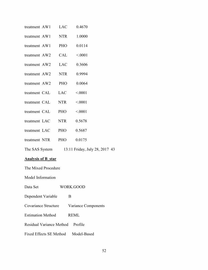
52
treatment AW1 LAC 0.4670
treatment AW1 NTR 1.0000
treatment AW1 PHO 0.0114
treatment AW2 CAL <.0001
treatment AW2 LAC 0.3606
treatment AW2 NTR 0.9994
treatment AW2 PHO 0.0064
treatment CAL LAC <.0001
treatment CAL NTR <.0001
treatment CAL PHO <.0001
treatment LAC NTR 0.5678
treatment LAC PHO 0.5687
treatment NTR PHO 0.0175
The SAS System 13:11 Friday, July 28, 2017 43
Analysis of B_star
The Mixed Procedure
Model Information
Data Set WORK.GOOD
Dependent Variable B
Covariance Structure Variance Components
Estimation Method REML
Residual Variance Method Profile
Fixed Effects SE Method Model-Based

53
Degrees of Freedom Method Containment
Class Level Information
Class Levels Values
roast_num 14 0 01 02 03 04 05 06 07 08 09
10 11 12 13
treatment 6 AW1 AW2 CAL LAC NTR PHO
Dimensions
Covariance Parameters 3
Columns in X 7
Columns in Z 93
Subjects 1
Max Obs per Subject 423
Number of Observations
Number of Observations Read 423
Number of Observations Used 423
Number of Observations Not Used 0
Iteration History
Iteration Evaluations -2 Res Log Like Criterion
0 1 1696.76347810
1 2 1616.40808211 0.00003243
2 1 1616.39358612 0.00000023
3 1 1616.39348630 0.00000000
Convergence criteria met.

54
The SAS System 13:11 Friday, July 28, 2017 44
Analysis of B_star
The Mixed Procedure
Covariance Parameter Estimates
Cov Parm Estimate
roast_num 0.6419
roast_num*treatment 0.4887
Residual 2.2175
Fit Statistics
-2 Res Log Likelihood 1616.4
AIC (Smaller is Better) 1622.4
AICC (Smaller is Better) 1622.5
BIC (Smaller is Better) 1624.3
Type 3 Tests of Fixed Effects
Num Den
Effect DF DF F Value Pr > F
treatment 5 60 42.63 <.0001
Least Squares Means
Standard
Effect treatment Estimate Error DF t Value Pr > |t|
treatment AW1 13.7292 0.3461 60 39.67 <.0001
treatment AW2 14.1771 0.3414 60 41.53 <.0001
treatment CAL 18.1973 0.3496 60 52.04 <.0001

55
treatment LAC 14.2598 0.3477 60 41.01 <.0001
treatment NTR 14.1562 0.3435 60 41.21 <.0001
treatment PHO 13.4534 0.3434 60 39.18 <.0001
Differences of Least Squares Means
Standard
Effect treatment _treatment Estimate Error DF t Value Pr > |t| Adjustment
treatment AW1 AW2 -0.4479 0.3751 60 -1.19 0.2372 Tukey-Kramer
treatment AW1 CAL -4.4682 0.3795 60 -11.77 <.0001 Tukey-Kramer
treatment AW1 LAC -0.5306 0.3785 60 -1.40 0.1662 Tukey-Kramer
treatment AW1 NTR -0.4270 0.3740 60 -1.14 0.2580 Tukey-Kramer
treatment AW1 PHO 0.2758 0.3743 60 0.74 0.4642 Tukey-Kramer
treatment AW2 CAL -4.0203 0.3784 60 -10.63 <.0001 Tukey-Kramer
treatment AW2 LAC -0.08269 0.3769 60 -0.22 0.8271 Tukey-Kramer
The SAS System 13:11 Friday, July 28, 2017 45
Analysis of B_star
The Mixed Procedure
Differences of Least Squares Means
Standard
Effect treatment _treatment Estimate Error DF t Value Pr > |t| Adjustment
treatment AW2 NTR 0.02085 0.3728 60 0.06 0.9556 Tukey-Kramer
treatment AW2 PHO 0.7237 0.3727 60 1.94 0.0569 Tukey-Kramer
treatment CAL LAC 3.9376 0.3818 60 10.31 <.0001 Tukey-Kramer
treatment CAL NTR 4.0411 0.3773 60 10.71 <.0001 Tukey-Kramer

56
treatment CAL PHO 4.7439 0.3776 60 12.56 <.0001 Tukey-Kramer
treatment LAC NTR 0.1035 0.3763 60 0.28 0.7841 Tukey-Kramer
treatment LAC PHO 0.8064 0.3759 60 2.14 0.0360 Tukey-Kramer
treatment NTR PHO 0.7028 0.3719 60 1.89 0.0636 Tukey-Kramer
Differences of Least Squares Means
Effect treatment _treatment Adj P
treatment AW1 AW2 0.8380
treatment AW1 CAL <.0001
treatment AW1 LAC 0.7259
treatment AW1 NTR 0.8618
treatment AW1 PHO 0.9765
treatment AW2 CAL <.0001
treatment AW2 LAC 0.9999
treatment AW2 NTR 1.0000
treatment AW2 PHO 0.3877
treatment CAL LAC <.0001
treatment CAL NTR <.0001
treatment CAL PHO <.0001
treatment LAC NTR 0.9998
treatment LAC PHO 0.2789
treatment NTR PHO 0.4183
The SAS System 13:11 Friday, July 28, 2017 56
Analysis of pH

57
The Mixed Procedure
Model Information
Data Set WORK.GOOD
Dependent Variable pH
Covariance Structure Variance Components
Estimation Method REML
Residual Variance Method Profile
Fixed Effects SE Method Model-Based
Degrees of Freedom Method Containment
Class Level Information
Class Levels Values
roast_num 13 01 02 03 04 05 06 07 08 09 10
11 12 13
treatment 6 AW1 AW2 CAL LAC NTR PHO
Dimensions
Covariance Parameters 3
Columns in X 7
Columns in Z 90
Subjects 1
Max Obs per Subject 442
Number of Observations
Number of Observations Read 442
Number of Observations Used 442

58
Number of Observations Not Used 0
Iteration History
Iteration Evaluations -2 Res Log Like Criterion
0 1 385.33780056
1 3 289.41176422 0.00134224
2 1 289.02933451 0.00005215
3 1 289.01560890 0.00000009
4 1 289.01558461 0.00000000
Convergence criteria met.
The SAS System 13:11 Friday, July 28, 2017 57
Analysis of pH
The Mixed Procedure
Covariance Parameter Estimates
Cov Parm Estimate
roast_num 0.02252
roast_num*treatment 0.02108
Residual 0.08970
Fit Statistics
-2 Res Log Likelihood 289.0
AIC (Smaller is Better) 295.0
AICC (Smaller is Better) 295.1
BIC (Smaller is Better) 296.7
Type 3 Tests of Fixed Effects

59
Num Den
Effect DF DF F Value Pr > F
treatment 5 59 152.53 <.0001
Least Squares Means
Standard
Effect treatment Estimate Error DF t Value Pr > |t|
treatment AW1 5.2763 0.06991 59 75.47 <.0001
treatment AW2 5.0849 0.06722 59 75.65 <.0001
treatment CAL 5.8905 0.06883 59 85.58 <.0001
treatment LAC 5.9143 0.06776 59 87.28 <.0001
treatment NTR 5.8829 0.06905 59 85.20 <.0001
treatment PHO 6.9886 0.06807 59 102.66 <.0001
Differences of Least Squares Mean
Standard
Effect treatment _treatment Estimate Error DF t Value Pr > |t| Adjustment
treatment AW1 AW2 0.1914 0.07678 59 2.49 0.0155 Tukey-Kramer
treatment AW1 CAL -0.6142 0.07848 59 -7.83 <.0001 Tukey-Kramer
treatment AW1 LAC -0.6380 0.07726 59 -8.26 <.0001 Tukey-Kramer
treatment AW1 NTR -0.6066 0.07847 59 -7.73 <.0001 Tukey-Kramer
treatment AW1 PHO -1.7123 0.07777 59 -22.02 <.0001 Tukey-Kramer
treatment AW2 CAL -0.8056 0.07606 59 -10.59 <.0001 Tukey-Kramer
treatment AW2 LAC -0.8294 0.07500 59 -11.06 <.0001 Tukey-Kramer
The SAS System 13:11 Friday, July 28, 2017 58

60
Analysis of pH
The Mixed Procedure
Differences of Least Squares Means
Standard
Effect treatment _treatment Estimate Error DF t Value Pr > |t| Adjustment
treatment AW2 NTR -0.7980 0.07618 59 -10.48 <.0001 Tukey-Kramer
treatment AW2 PHO -1.9038 0.07539 59 -25.25 <.0001 Tukey-Kramer
treatment CAL LAC -0.02379 0.07658 59 -0.31 0.7572 Tukey-Kramer
treatment CAL NTR 0.007625 0.07770 59 0.10 0.9222 Tukey-Kramer
treatment CAL PHO -1.0981 0.07682 59 -14.29 <.0001 Tukey-Kramer
treatment LAC NTR 0.03142 0.07667 59 0.41 0.6835 Tukey-Kramer
treatment LAC PHO -1.0743 0.07586 59 -14.16 <.0001 Tukey-Kramer
treatment NTR PHO -1.1057 0.07700 59 -14.36 <.0001 Tukey-Kramer
Differences of Least Squares Means
Effect treatment _treatment Adj P
treatment AW1 AW2 0.1427
treatment AW1 CAL <.0001
treatment AW1 LAC <.0001
treatment AW1 NTR <.0001
treatment AW1 PHO <.0001
treatment AW2 CAL <.0001
treatment AW2 LAC <.0001
treatment AW2 NTR <.0001

61
treatment AW2 PHO <.0001
treatment CAL LAC 0.9996
treatment CAL NTR 1.0000
treatment CAL PHO <.0001
treatment LAC NTR 0.9984
treatment LAC PHO <.0001
treatment NTR PHO <.0001
The SAS System 13:11 Friday, July 28, 2017 68
Analysis of Difference
The Mixed Procedure
Model Information
Data Set WORK.GOOD
Dependent Variable Difference
Covariance Structure Variance Components
Estimation Method REML
Residual Variance Method Profile
Fixed Effects SE Method Model-Based
Degrees of Freedom Method Containment
Class Level Informatio
Class Levels Values
roast_num 16 01 02 03 04 05 06 07 08 09 10
11 12 13 5 7 8
treatment 6 AW1 AW2 CAL LAC NTR PHO

62
Dimensions
Covariance Parameters 3
Columns in X 7
Columns in Z 97
Subjects 1
Max Obs per Subject 422
Number of Observations
Number of Observations Read 422
Number of Observations Used 422
Number of Observations Not Used 0
Iteration History
Iteration Evaluations -2 Res Log Like Criterion
0 1 2059.17520984
1 2 2020.78743165 0.22067827
2 3 2015.17839263 .
3 1 1972.79182564 0.03234612
4 1 1946.99105320 0.01974043
5 1 1931.64129158 0.01132416
6 1 1923.02193774 0.00581922
7 1 1918.69029247 0.00245977
8 1 1916.91582319 0.00071313
The SAS System 13:11 Friday, July 28, 2017 69
Analysis of Difference

63
The Mixed Procedure
Iteration History
Iteration Evaluations -2 Res Log Like Criterion
9 1 1916.42813935 0.00009423
10 1 1916.36886078 0.00000229
11 1 1916.36751662 0.00000000
Convergence criteria met.
Covariance Parameter Estimates
Cov Parm Estimate
roast_num 58.5390
roast_num*treatment 0.3275
Residual 4.3283
Fit Statistics
-2 Res Log Likelihood 1916.4
AIC (Smaller is Better) 1922.4
AICC (Smaller is Better) 1922.4
BIC (Smaller is Better) 1924.7
Type 3 Tests of Fixed Effects
Num Den
Effect DF DF F Value Pr > F
treatment 5 60 72.28 <.0001
Least Squares Means
Standard

64
Effect treatment Estimate Error DF t Value Pr > |t|
treatment AW1 15.2339 1.9417 60 7.85 <.0001
treatment AW2 14.6047 1.9498 60 7.49 <.0001
treatment CAL 16.8317 1.9513 60 8.63 <.0001
treatment LAC 16.7133 1.9486 60 8.58 <.0001
treatment NTR 12.9773 1.9504 60 6.65 <.0001
treatment PHO 10.1558 1.9496 60 5.21 <.0001
The SAS System 13:11 Friday, July 28, 2017 70
Analysis of Difference
The Mixed Procedure
Differences of Least Squares Means
Standard
Effect treatment _treatment Estimate Error DF t Value Pr > |t| Adjustment
treatment AW1 AW2 0.6292 0.4207 60 1.50 0.1400 Tukey-Kramer
treatment AW1 CAL -1.5977 0.4287 60 -3.73 0.0004 Tukey-Kramer
treatment AW1 LAC -1.4794 0.4144 60 -3.57 0.0007 Tukey-Kramer
treatment AW1 NTR 2.2566 0.4227 60 5.34 <.0001 Tukey-Kramer
treatment AW1 PHO 5.0781 0.4200 60 12.09 <.0001 Tukey-Kramer
treatment AW2 CAL -2.2270 0.4291 60 -5.19 <.0001 Tukey-Kramer
treatment AW2 LAC -2.1086 0.4161 60 -5.07 <.0001 Tukey-Kramer
treatment AW2 NTR 1.6274 0.4242 60 3.84 0.0003 Tukey-Kramer
treatment AW2 PHO 4.4489 0.4208 60 10.57 <.0001 Tukey-Kramer
treatment CAL LAC 0.1184 0.4243 60 0.28 0.7812 Tukey-Kramer
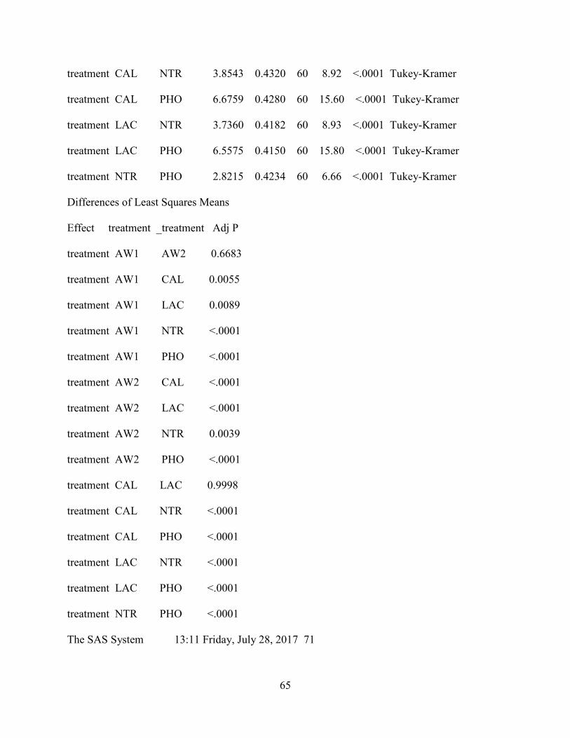
65
treatment CAL NTR 3.8543 0.4320 60 8.92 <.0001 Tukey-Kramer
treatment CAL PHO 6.6759 0.4280 60 15.60 <.0001 Tukey-Kramer
treatment LAC NTR 3.7360 0.4182 60 8.93 <.0001 Tukey-Kramer
treatment LAC PHO 6.5575 0.4150 60 15.80 <.0001 Tukey-Kramer
treatment NTR PHO 2.8215 0.4234 60 6.66 <.0001 Tukey-Kramer
Differences of Least Squares Means
Effect treatment _treatment Adj P
treatment AW1 AW2 0.6683
treatment AW1 CAL 0.0055
treatment AW1 LAC 0.0089
treatment AW1 NTR <.0001
treatment AW1 PHO <.0001
treatment AW2 CAL <.0001
treatment AW2 LAC <.0001
treatment AW2 NTR 0.0039
treatment AW2 PHO <.0001
treatment CAL LAC 0.9998
treatment CAL NTR <.0001
treatment CAL PHO <.0001
treatment LAC NTR <.0001
treatment LAC PHO <.0001
treatment NTR PHO <.0001
The SAS System 13:11 Friday, July 28, 2017 71

66
Analysis of Percent Loss
The Mixed Procedure
Model Information
Data Set WORK.GOOD
Dependent Variable percent_loss
Covariance Structure Variance Components
Estimation Method REML
Residual Variance Method Profile
Fixed Effects SE Method Model-Based
Degrees of Freedom Method Containment
Class Level Information
Class Levels Values
roast_num 16 01 02 03 04 05 06 07 08 09 10
11 12 13 5 7 8
treatment 6 AW1 AW2 CAL LAC NTR PHO
Dimensions
Covariance Parameters 3
Columns in X 7
Columns in Z 97
Subjects 1
Max Obs per Subject 422
Number of Observations
Number of Observations Read 422

67
Number of Observations Used 422
Number of Observations Not Used 0
Iteration History
Iteration Evaluations -2 Res Log Like Criterion
0 1 2930.72653354
1 2 2882.32125392 5.75891726
2 1 2850.53347033 2.18999730
3 3 2835.24856259 .
4 1 2790.86772424 0.02029831
5 1 2763.69420387 0.01242968
6 1 2747.33607263 0.00718642
7 1 2738.02921952 0.00375142
8 1 2733.26029633 0.00163612
The SAS System 13:11 Friday, July 28, 2017 72
Analysis of Percent Loss
The Mixed Procedure
Iteration History
Iteration Evaluations -2 Res Log Like Criterion
9 1 2731.23759578 0.00050584
10 1 2730.64215266 0.00007672
11 1 2730.55880894 0.00000251
12 1 2730.55628130 0.00000000
Convergence criteria met.

68
Covariance Parameter Estimates
Cov Parm Estimate
roast_num 619.98
roast_num*treatment 3.5554
Residual 29.5023
Fit Statistics
-2 Res Log Likelihood 2730.6
AIC (Smaller is Better) 2736.6
AICC (Smaller is Better) 2736.6
BIC (Smaller is Better) 2738.9
Type 3 Tests of Fixed Effects
Num Den
Effect DF DF F Value Pr > F
treatment 5 60 83.48 <.0001
Least Squares Means
Standard
Effect treatment Estimate Error DF t Value Pr > |t|
treatment AW1 47.6103 6.2927 60 7.57 <.0001
treatment AW2 45.9779 6.3130 60 7.28 <.0001
treatment CAL 51.1462 6.3162 60 8.10 <.0001
treatment LAC 51.3134 6.3107 60 8.13 <.0001
treatment NTR 40.4756 6.3144 60 6.41 <.0001
treatment PHO 31.1844 6.3127 60 4.94 <.0001

69
The SAS System 13:11 Friday, July 28, 2017 73
Analysis of Percent Loss
The Mixed Procedure
Differences of Least Squares Means
Standard
Effect treatment _treatment Estimate Error DF t Value Pr > |t| Adjustment
treatment AW1 AW2 1.6325 1.1906 60 1.37 0.1754 Tukey-Kramer
treatment AW1 CAL -3.5359 1.2097 60 -2.92 0.0049 Tukey-Kramer
treatment AW1 LAC -3.7031 1.1767 60 -3.15 0.0026 Tukey-Kramer
treatment AW1 NTR 7.1347 1.1965 60 5.96 <.0001 Tukey-Kramer
treatment AW1 PHO 16.4259 1.1895 60 13.81 <.0001 Tukey-Kramer
treatment AW2 CAL -5.1683 1.2096 60 -4.27 <.0001 Tukey-Kramer
treatment AW2 LAC -5.3356 1.1795 60 -4.52 <.0001 Tukey-Kramer
treatment AW2 NTR 5.5023 1.1991 60 4.59 <.0001 Tukey-Kramer
treatment AW2 PHO 14.7934 1.1901 60 12.43 <.0001 Tukey-Kramer
treatment CAL LAC -0.1672 1.1991 60 -0.14 0.8895 Tukey-Kramer
treatment CAL NTR 10.6706 1.2179 60 8.76 <.0001 Tukey-Kramer
treatment CAL PHO 19.9618 1.2075 60 16.53 <.0001 Tukey-Kramer
treatment LAC NTR 10.8379 1.1860 60 9.14 <.0001 Tukey-Kramer
treatment LAC PHO 20.1290 1.1775 60 17.09 <.0001 Tukey-Kramer
treatment NTR PHO 9.2911 1.1976 60 7.76 <.0001 Tukey-Kramer
Differences of Least Squares Means
Effect treatment _treatment Adj P

70
treatment AW1 AW2 0.7438
treatment AW1 CAL 0.0527
treatment AW1 LAC 0.0294
treatment AW1 NTR <.0001
treatment AW1 PHO <.0001
treatment AW2 CAL 0.0010
treatment AW2 LAC 0.0004
treatment AW2 NTR 0.0003
treatment AW2 PHO <.0001
treatment CAL LAC 1.0000
treatment CAL NTR <.0001
treatment CAL PHO <.0001
treatment LAC NTR <.0001
treatment LAC PHO <.0001
treatment NTR PHO <.0001
The SAS System 14:10 Thursday, August 3, 2017 1
The SAS System 14:10 Thursday, August 3, 2017 11
Analysis of L_star
The Mixed Procedure
Model Information
Data Set WORK.GOOD
Dependent Variable L
Covariance Structure Variance Components

71
Estimation Method REML
Residual Variance Method Profile
Fixed Effects SE Method Model-Based
Degrees of Freedom Method Containment
Class Level Information
Class Levels Values
roast_num 13 01 02 03 04 05 06 07 08 09 10
11 12 13
treatment 6 AW1 AW2 CAL LAC NTR PHO
Dimensions
Covariance Parameters 3
Columns in X 7
Columns in Z 85
Subjects 1
Max Obs per Subject 481
Number of Observations
Number of Observations Read 481
Number of Observations Used 481
Number of Observations Not Used 0
Iteration History
Iteration Evaluations -2 Res Log Like Criterion
0 1 3114.80564219

72
1 3 3069.01482958 0.00000021
2 1 3069.01459909 0.00000000
Convergence criteria met.
The SAS System 14:10 Thursday, August 3, 2017 12
Analysis of L_star
The Mixed Procedure
Covariance Parameter Estimates
Cov Parm Estimate
roast_num 5.0368
roast_num*treatment 1.8243
Residual 32.6313
Fit Statistics
-2 Res Log Likelihood 3069.0
AIC (Smaller is Better) 3075.0
AICC (Smaller is Better) 3075.1
BIC (Smaller is Better) 3076.7
Type 3 Tests of Fixed Effects
Num Den
Effect DF DF F Value Pr > F
treatment 5 54 9.96 <.0001
Least Squares Means
Standard
Effect treatment Estimate Error DF t Value Pr > |t|

73
treatment AW1 40.1934 0.9650 54 41.65 <.0001
treatment AW2 41.4492 1.2083 54 34.30 <.0001
treatment CAL 38.3509 0.9647 54 39.75 <.0001
treatment LAC 43.3548 0.9601 54 45.16 <.0001
treatment NTR 42.5889 0.9453 54 45.06 <.0001
treatment PHO 44.9239 0.9853 54 45.60 <.000
Differences of Least Squares Means
Standard
Effect treatment _treatment Estimate Error DF t Value Pr > |t| Adjustment
treatment AW1 AW2 -1.2557 1.2797 54 -0.98 0.3308 Tukey-Kramer
treatment AW1 CAL 1.8425 1.0345 54 1.78 0.0805 Tukey-Kramer
treatment AW1 LAC -3.1614 1.0333 54 -3.06 0.0034 Tukey-Kramer
treatment AW1 NTR -2.3955 1.0169 54 -2.36 0.0221 Tukey-Kramer
treatment AW1 PHO -4.7305 1.0542 54 -4.49 <.0001 Tukey-Kramer
treatment AW2 CAL 3.0983 1.2818 54 2.42 0.0191 Tukey-Kramer
treatment AW2 LAC -1.9056 1.2779 54 -1.49 0.1417 Tukey-Kramer
The SAS System 14:10 Thursday, August 3, 2017 13
Analysis of L_star
The Mixed Procedure
Differences of Least Squares Means
Standard
Effect treatment _treatment Estimate Error DF t Value Pr > |t| Adjustment
treatment AW2 NTR -1.1398 1.2642 54 -0.90 0.3713 Tukey-Kramer

74
treatment AW2 PHO -3.4748 1.2885 54 -2.70 0.0093 Tukey-Kramer
treatment CAL LAC -5.0039 1.0318 54 -4.85 <.0001 Tukey-Kramer
treatment CAL NTR -4.2380 1.0176 54 -4.16 0.0001 Tukey-Kramer
treatment CAL PHO -6.5730 1.0573 54 -6.22 <.0001 Tukey-Kramer
treatment LAC NTR 0.7658 1.0160 54 0.75 0.4543 Tukey-Kramer
treatment LAC PHO -1.5691 1.0535 54 -1.49 0.1422 Tukey-Kramer
treatment NTR PHO -2.3350 1.0392 54 -2.25 0.0287 Tukey-Kramer
Differences of Least Squares Means
Effect treatment _treatment Adj P
treatment AW1 AW2 0.9219
treatment AW1 CAL 0.4863
treatment AW1 LAC 0.0383
treatment AW1 NTR 0.1904
treatment AW1 PHO 0.0005
treatment AW2 CAL 0.1687
treatment AW2 LAC 0.6712
treatment AW2 NTR 0.9444
treatment AW2 PHO 0.0925
treatment CAL LAC 0.0002
treatment CAL NTR 0.0015
treatment CAL PHO <.0001
treatment LAC NTR 0.9739
treatment LAC PHO 0.6723

75
treatment NTR PHO 0.2340
The SAS System 14:10 Thursday, August 3, 2017 14
Analysis of A_star
The Mixed Procedure
Model Information
Data Set WORK.GOOD
Dependent Variable A
Covariance Structure Variance Components
Estimation Method REML
Residual Variance Method Profile
Fixed Effects SE Method Model-Based
Degrees of Freedom Method Containment
Class Level Information
Class Levels Values
roast_num 13 01 02 03 04 05 06 07 08 09 10
11 12 13
treatment 6 AW1 AW2 CAL LAC NTR PHO
Dimensions
Covariance Parameters 3
Columns in X 7
Columns in Z 85
Subjects 1
Max Obs per Subject 481

76
Number of Observations
Number of Observations Read 481
Number of Observations Used 481
Number of Observations Not Used 0
Iteration History
Iteration Evaluations -2 Res Log Like Criterion
0 1 2299.12804987
1 3 2274.94753058 0.00003877
2 1 2274.91922503 0.00000017
3 1 2274.91910733 0.00000000
Convergence criteria met.
The SAS System 14:10 Thursday, August 3, 2017 15
Analysis of A_star
The Mixed Procedure
Covariance Parameter Estimates
Cov Parm Estimate
roast_num 0.4946
roast_num*treatment 0.3934
Residual 6.1801
Fit Statistics
-2 Res Log Likelihood 2274.9
AIC (Smaller is Better) 2280.9
AICC (Smaller is Better) 2281.0

77
BIC (Smaller is Better) 2282.6
Type 3 Tests of Fixed Effects
Num Den
Effect DF DF F Value Pr > F
treatment 5 54 11.79 <.0001
Least Squares Means
Standard
Effect treatment Estimate Error DF t Value Pr > |t|
treatment AW1 7.3382 0.3805 54 19.29 <.0001
treatment AW2 6.8444 0.4960 54 13.80 <.0001
treatment CAL 10.2431 0.3803 54 26.93 <.0001
treatment LAC 9.1069 0.3781 54 24.08 <.0001
treatment NTR 8.7361 0.3709 54 23.55 <.0001
treatment PHO 9.0315 0.3903 54 23.14 <.0001
Differences of Least Squares Means
Standard
Effect treatment _treatment Estimate Error DF t Value Pr > |t| Adjustment
treatment AW1 AW2 0.4938 0.5639 54 0.88 0.3851 Tukey-Kramer
treatment AW1 CAL -2.9049 0.4591 54 -6.33 <.0001 Tukey-Kramer
treatment AW1 LAC -1.7687 0.4583 54 -3.86 0.0003 Tukey-Kramer
treatment AW1 NTR -1.3980 0.4515 54 -3.10 0.0031 Tukey-Kramer
treatment AW1 PHO -1.6934 0.4675 54 -3.62 0.0006 Tukey-Kramer
treatment AW2 CAL -3.3987 0.5646 54 -6.02 <.0001 Tukey-Kramer

78
treatment AW2 LAC -2.2625 0.5630 54 -4.02 0.0002 Tukey-Kramer
The SAS System 14:10 Thursday, August 3, 2017 16
Analysis of A_star
The Mixed Procedure
Differences of Least Squares Means
Standard
Effect treatment _treatment Estimate Error DF t Value Pr > |t| Adjustment
treatment AW2 NTR -1.8917 0.5573 54 -3.39 0.0013 Tukey-Kramer
treatment AW2 PHO -2.1872 0.5683 54 -3.85 0.0003 Tukey-Kramer
treatment CAL LAC 1.1362 0.4578 54 2.48 0.0162 Tukey-Kramer
treatment CAL NTR 1.5069 0.4517 54 3.34 0.0015 Tukey-Kramer
treatment CAL PHO 1.2115 0.4686 54 2.59 0.0125 Tukey-Kramer
treatment LAC NTR 0.3707 0.4508 54 0.82 0.4145 Tukey-Kramer
treatment LAC PHO 0.07534 0.4669 54 0.16 0.8724 Tukey-Kramer
treatment NTR PHO -0.2954 0.4608 54 -0.64 0.5242 Tukey-Kramer
Differences of Least Squares Means
Effect treatment _treatment Adj P
treatment AW1 AW2 0.9507
treatment AW1 CAL <.0001
treatment AW1 LAC 0.0040
treatment AW1 NTR 0.0348
treatment AW1 PHO 0.0081
treatment AW2 CAL <.0001

79
treatment AW2 LAC 0.0024
treatment AW2 NTR 0.0155
treatment AW2 PHO 0.0041
treatment CAL LAC 0.1478
treatment CAL NTR 0.0183
treatment CAL PHO 0.1185
treatment LAC NTR 0.9621
treatment LAC PHO 1.0000
treatment NTR PHO 0.9873
The SAS System 14:10 Thursday, August 3, 2017 17
Analysis of B_star
The Mixed Procedure
Model Information
Data Set WORK.GOOD
Dependent Variable B
Covariance Structure Variance Components
Estimation Method REML
Residual Variance Method Profile
Fixed Effects SE Method Model-Based
Degrees of Freedom Method Containment
Class Level Information
Class Levels Values
roast_num 13 01 02 03 04 05 06 07 08 09 10

80
11 12 13
treatment 6 AW1 AW2 CAL LAC NTR PHO
Dimensions
Covariance Parameters 3
Columns in X 7
Columns in Z 85
Subjects 1
Max Obs per Subject 481
Number of Observations
Number of Observations Read 481
Number of Observations Used 481
Number of Observations Not Used 0
Iteration History
Iteration Evaluations -2 Res Log Like Criterion
0 1 2271.78562366
1 3 2248.88249469 0.00000214
2 1 2248.88099186 0.00000000
Convergence criteria met.
The SAS System 14:10 Thursday, August 3, 2017 18
Analysis of B_star
The Mixed Procedure
Covariance Parameter Estimates
Cov Parm Estimate

81
roast_num 0.3684
roast_num*treatment 0.4913
Residual 5.8076
Fit Statistics
-2 Res Log Likelihood 2248.9
AIC (Smaller is Better) 2254.9
AICC (Smaller is Better) 2254.9
BIC (Smaller is Better) 2256.6
Type 3 Tests of Fixed Effects
Num Den
Effect DF DF F Value Pr > F
treatment 5 54 13.12 <.0001
Least Squares Means
Standard
Effect treatment Estimate Error DF t Value Pr > |t|
treatment AW1 15.0550 0.3724 54 40.42 <.0001
treatment AW2 15.5306 0.4891 54 31.75 <.0001
treatment CAL 16.8479 0.3722 54 45.27 <.0001
treatment LAC 17.5609 0.3699 54 47.47 <.0001
treatment NTR 17.1602 0.3629 54 47.28 <.0001
treatment PHO 18.4622 0.3825 54 48.27 <.0001
Differences of Least Squares Means
Standard

82
Effect treatment _treatment Estimate Error DF t Value Pr > |t| Adjustment
treatment AW1 AW2 -0.4756 0.5693 54 -0.84 0.4072 Tukey-Kramer
treatment AW1 CAL -1.7929 0.4675 54 -3.84 0.0003 Tukey-Kramer
treatment AW1 LAC -2.5059 0.4666 54 -5.37 <.0001 Tukey-Kramer
treatment AW1 NTR -2.1052 0.4603 54 -4.57 <.0001 Tukey-Kramer
treatment AW1 PHO -3.4072 0.4759 54 -7.16 <.0001 Tukey-Kramer
treatment AW2 CAL -1.3174 0.5698 54 -2.31 0.0246 Tukey-Kramer
treatment AW2 LAC -2.0303 0.5683 54 -3.57 0.0008 Tukey-Kramer
The SAS System 14:10 Thursday, August 3, 2017 19
Analysis of B_star
The Mixed Procedure
Differences of Least Squares Means
Standard
Effect treatment _treatment Estimate Error DF t Value Pr > |t| Adjustment
treatment AW2 NTR -1.6296 0.5629 54 -2.89 0.0055 Tukey-Kramer
treatment AW2 PHO -2.9316 0.5739 54 -5.11 <.0001 Tukey-Kramer
treatment CAL LAC -0.7129 0.4660 54 -1.53 0.1319 Tukey-Kramer
treatment CAL NTR -0.3123 0.4604 54 -0.68 0.5005 Tukey-Kramer
treatment CAL PHO -1.6143 0.4766 54 -3.39 0.0013 Tukey-Kramer
treatment LAC NTR 0.4007 0.4593 54 0.87 0.3869 Tukey-Kramer
treatment LAC PHO -0.9013 0.4750 54 -1.90 0.0631 Tukey-Kramer
treatment NTR PHO -1.3020 0.4693 54 -2.77 0.0076 Tukey-Kramer
Differences of Least Squares Means

83
Effect treatment _treatment Adj P
treatment AW1 AW2 0.9595
treatment AW1 CAL 0.0043
treatment AW1 LAC <.0001
treatment AW1 NTR 0.0004
treatment AW1 PHO <.0001
treatment AW2 CAL 0.2073
treatment AW2 LAC 0.0093
treatment AW2 NTR 0.0579
treatment AW2 PHO <.0001
treatment CAL LAC 0.6470
treatment CAL NTR 0.9836
treatment CAL PHO 0.0159
treatment LAC NTR 0.9515
treatment LAC PHO 0.4147
treatment NTR PHO 0.0773

84
Sensory Comments P r o d u c t s 1 - 935 935 No Treatment 2 - 146 146 Acid Whey 3 - 213 213 Calcium 4 - 527 527 Lactic Acid 5 - 798 798 Phosphate R e s u l t s 1 17 1-935 The taste was absent while the texture seemed unsettling. This was my least favorite
of the selections today.
1 19 1-935 tasted very good
1 40 1-935 It was really hard to answer all of these questions with the amount of sample that we
had. I didn't know how many more questions I was going to have to answer and two bites was
not enough to remember everything. If I could answer all of the questions at the same time, then
I could have gone through and rated everything about one sample, and then move on to the next
sample. ...I didn't know I was going to have to rank them, I think that is close to my opinon, but
there were so many samples and so many questions.
1 45 1-935 This sample is slightly over cooked. But still the best.
1 48 1-935 GReat. Could maybe use a touch of tenerizer or pounding.
1 51 1-935 this sample is the only one that really smelled like a steak to me.
1 55 1-935 This was the best of the five...
1 66 1-935 This sample was the best tasting as far as flavor, tenderness, and juiciness.
1 76 1-935 935 had the most/best flavor of the samples that I enjoyed.
1 90 1-935 I liked the doneness and flavor of 935 the best, but in all cases, l was surprised by
how watery all the steak tasted.

85
1 101 1-935 While 935 appeared the darkest, I thought it had the best flavor and about the right
level of juicyness.
1 107 1-935 This might've tasted the best by just a tiny bit, but the overall presentation brought it
down to 2nd for me.
1 109 1-935 I like it! good presentation and flavor, needed to be juicy to reach perfection.
1 14 2-146 Sample 146 was near perfect! It was juicier and tasted better - but wasn't as raw as
sample 798
1 19 2-146 tasted very good
1 33 2-146 very tough and difficult to chew
1 48 2-146 REALLY chewey
1 57 2-146 I like the outter sear.
1 71 2-146 Very well prepared and had an excellent taste.
1 80 2-146 This one felt like the clear winner to me. The others were either too dry or too bland.
1 102 2-146 Best overall sample, but all samples could have used a little salt.
1 109 2-146 Is correct the point of cooking.
1 18 3-213 A little on the rare side.
1 19 3-213 too much grizzel
1 38 3-213 too pink for me to eat :(
1 39 3-213 Looked too raw to me.
1 48 3-213 NExt best. Not as chewey as the other 3.
1 49 3-213 A little to red for me - didn't seem well done.
1 57 3-213 Very pale.
1 65 3-213 #213 wasn't cooked very well, but it had the best flavor.
86
1 109 3-213 Needs to bleed to be juicy. If it is 'rare'
1 19 4-527 tasted very good
1 37 4-527 Seems too rare.
1 38 4-527 Too pink to eat, and you can see a small vessel :(
1 48 4-527 chewy
1 49 4-527 Way too red, color turned me off a bit.
1 57 4-527 appearance is just right.
1 71 4-527 While I wouldn't have considered it as ''well done,'' this sample was exceptionally
good. The taste and moistness were very good.
1 89 4-527 Best one for juciness and flavor
1 107 4-527 This had hardly any taste and was way too rare for me.
1 109 4-527 It is assumed that needs to be juicy. It was not tender.
1 15 5-798 Looks scary. I think I always expect more color.
1 16 5-798 Sample 798 one looks under cooked, I had to really talk myself into eating it. There's
a strange sheen to the meat. The seared edges add flavor, this one didn't offer that seared flavor.
1 18 5-798 Does not appear cooked enough. Appears rare and too much juicy liquid.
1 19 5-798 Little bloodier but very good
1 48 5-798 chewy, but not quite as band as the last 2
1 49 5-798 Closer to well done, but still a little too pink.
1 53 5-798 This is the only sample I deliberately did not finish.
1 57 5-798 Very pale.
1 58 5-798 This one was my favorite
1 83 5-798 I felt this one was over cooked.

87
1 89 5-798 Dry
1 100 5-798 it was an off flavor not exactly meat off flavor
1 102 5-798 Toughest and driest of the lot.
1 107 5-798 This was my second favorite in taste by just a tiny bit, but the overall presentation
(appearance, juiciness, aroma, flavor, etc) made it the best for me.