Embed Size (px)
Citation preview

I. Introduction
The global financial crisis in 2008 caused large government deficits, leading to an increase in government debt. Many countries are currently attempting to find a balance between using extensive fiscal policy and returning to a sustainable path for public finances without
Kwang Jo Jeong, Head of the IMF Team, International Monetary System Division, Ministry of Strategy and Finance, South Korea. (E-mail): [email protected], (Tel): +82 44 215 4840, (Fax): +82 44 215 8139.
I am grateful to Professor Soyoung Kim, Anonymous referees and Editorial Manager of SJE Jin-hee Choi for useful comments and suggestions.
[Seoul Journal of Economics 2017, Vol. 30, No. 1]
Effects of Fiscal Consolidation in 18 OECD Countries
Kwang Jo Jeong
This paper estimates the effects of fiscal consolidation on economic growth using panel datasets from 18 Organization for Economic Cooperation and Development (OECD) countries. The estimates of dynamic panel data Generalized Method of Moment (GMM) analysis show that fiscal consolidation is unlikely to be expansionary for GDP growth. Both Arellano-Bond difference GMM estimation and Blundell-Bond system GMM estimation suggest that fiscal consolidation exert negative effects on economic growth. Results do not support the expansionary fiscal consolidation hypothesis. In particular, our analyses find that fiscal consolidations during high debt-to-GDP ratios, based on spending cuts, or with high sovereign default risk exert less negative effects on economic growth than those during low debt-to-GDP ratios, based on tax hikes, or with low sovereign default risk.
Keywords: Fiscal consolidation, Economic growth, Debt-to-GDP ratio, Sovereign default risk
JEL Classification: E61, E62, H62, H63, H87
52 SEOUL JOURNAL OF ECONOMICS
hurting economic recovery based on expansionary fiscal consolidation hypothesis. Not all countries have accepted this hypothesis, and a strong disagreement over the necessity for harsh and abrupt austerity measures continues to exist.
Historically, efforts to provide evidence in favor of expansionary fiscal consolidation have been consistent. The possibility of “non-Keynesian expansionary effects” resulting from restrictive fiscal policies was first raised by Barro (1974). This issue drew more interest after Giavazzi, and Pagano (1990) provided evidence of expansionary fiscal consolidation in Denmark (1983–86) and Ireland (1987–89).
Several recently observed examples trigger doubt about the appropriateness of fiscal consolidation and raise suspicion that such activity undermines economy. In the aftermath of the global financial crisis in 2008, the UK began a fiscal austerity program to reduce its deficit from the third quarter of 2010. Conservative politicians argued that fiscal consolidation could enhance growth, and they underlined the need to avoid rising debt costs as a key motivation in undertaking this program. However, in the last quarter of 2011 and first quarter of 2012, the UK suffered from its first double-dip recession in 37 years. The economy of the UK unexpectedly slumped by 0.2 per cent of GDP in the first quarter of 2012. This slump followed a fall of 0.3 per cent in the final quarter of 2011.
In this context, this paper reviews the theoretical and empirical literature that has investigated the conditions under which fiscal consolidation is effective in enhancing economic growth and reducing public debt (or fiscal deficit). We adopted a policy action-based approach instead of using a cyclically adjusted primary balance (CAPB)-based approach, which was commonly used in previous research. A policy action-based approach was newly proposed by the IMF (IMF 2010; Leigh et al. 2011) to improve the function of identifying fiscal consolidation episodes.
Unlike the study of the IMF (IMF 2010; Leigh et al. 2011), this paper addresses the endogeneity problem in the analysis using a dynamic panel GMM model. The fixed-effects dynamic panel model of the IMF (Leigh et al. 2011) suffers from the endogeneity problem because it simply uses OLS estimates, which are inconsistent because of the correlation of the lagged dependent variable with the error term.
This paper contributes to uncovering the effects of fiscal consolidation on economic growth. This paper is organized as follows. Section II
53Macro econoMic effects of fiscal consolidation
reviews the theoretical and empirical literature on the effects of fiscal consolidation. Section III identifies fiscal consolidation episodes and specifies model. Section IV explains the data. Section V shows empirical results. Section VI tests the robustness of the results. Section VII concludes.
II. Literature Review
A. Theoretical Approach
Keynesian analysis insists that fiscal consolidation inevitably leads to a contraction of aggregate demand and reduces GDP. It disagrees with the non-Keynesian effects that fiscal austerity is necessary to overcome economic crisis even if the world economy remains deeply depressed. Keynesians argue that if an economy performs well following government spending cuts, then this performance is because the business cycle has picked up or the government monetary policy is more expansionary at the time.
Over the last two decades, the Keynesian view has been contended. Using the cases of Denmark and Ireland, Giavazzi, and Pagano (1990)1 suggest that fiscal consolidation can be expansionary, because the GDP of these two countries increased after fiscal tightening. Alesina, and Ardagna (2010, 2012) also show that spending-based reduction has caused smaller recession and occasionally growth in GDP.
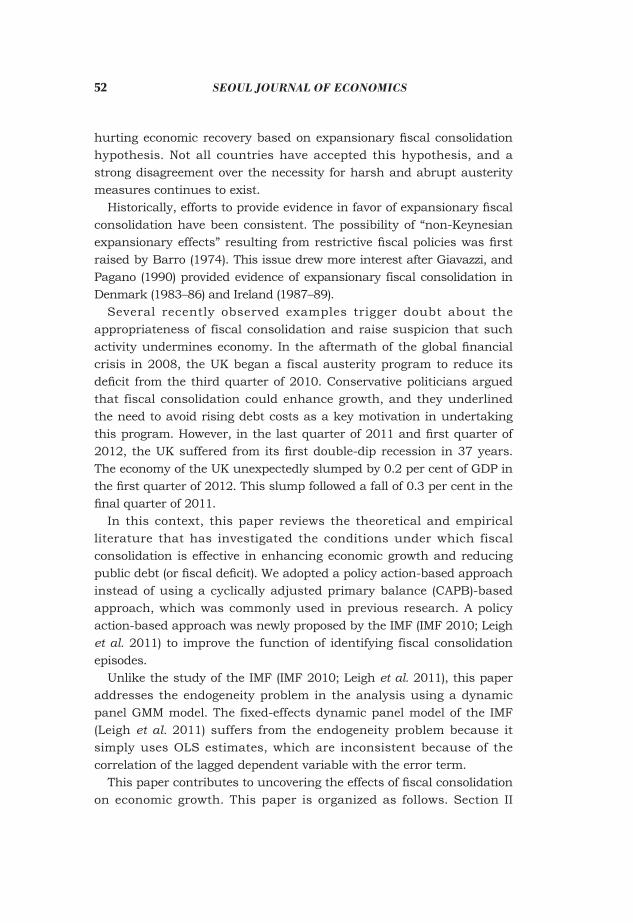
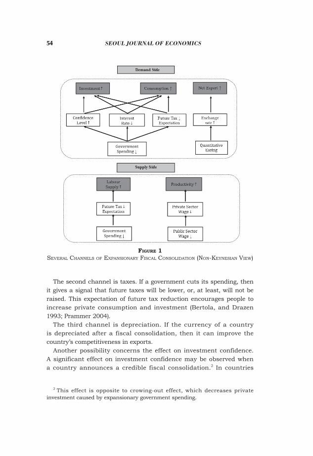
Several channels can explain how fiscal consolidation may not be recessionary or may occasionally be expansionary. Theoretically, expansionary effects of fiscal consolidation can go through both the demand and supply sides (Figure 1).
On the demand side, the first channel is a rapid reduction of interest rates. If a government reduces its spending and reduces the deficit, then people worry less about the future and apply a lower risk premium to the country’s government debt. That is, reduced interest rates can stimulate aggregate demand through both private investment (McDermott, and Wescott 1996) and consumption because of the positive wealth effect in the private sector (Giavazzi, and Pagano 1990).
1 Blanchard (1990) extrapolates from Giavazzi and Pagano’s analysis to suggest that fiscal consolidation can raise investment, aggregate demand, and output.
54 SEOUL JOURNAL OF ECONOMICS
The second channel is taxes. If a government cuts its spending, then it gives a signal that future taxes will be lower, or, at least, will not be raised. This expectation of future tax reduction encourages people to increase private consumption and investment (Bertola, and Drazen 1993; Prammer 2004).
The third channel is depreciation. If the currency of a country is depreciated after a fiscal consolidation, then it can improve the country’s competitiveness in exports.
Another possibility concerns the effect on investment confidence. A significant effect on investment confidence may be observed when a country announces a credible fiscal consolidation.2 In countries
2 This effect is opposite to crowing-out effect, which decreases private investment caused by expansionary government spending.
Figure 1Several ChannelS of expanSionary fiSCal ConSolidation (non-KeyneSian view)
55Macro econoMic effects of fiscal consolidation
such as the US, an increase in confidence among investors is crucial to reduce the negative effects of fiscal consolidation. If a government reduces uncertainty about the future fiscal policy, then investors will be less hesitant about investing their money in the country (Alesina, and Ardagna 2010, 2012).
On the supply side, the expansionary effects of fiscal consolidation work through the labor market. The first channel is the private-sector wage-depressing effect. If public sector wages are kept down, then wage-depressing agreements in the private sector of the economy may follow. Finally, competitiveness may increase, thus improving productivity.3
The second channel is taxes. If a government cuts its spending, then it signals tax reductions in the future. This expectation of future tax reductions will encourage employees to increase their labor supply, resulting in a decrease of pre-tax real wage. This decrease signifies lower labor unit costs for firms and considerable gain in competitiveness.
Despite the various types of theoretical support for expansionary fiscal consolidation, opposition to non-Keynesian expansionary effects has been growing since countries attempted to implement austerity measures early in 2010. For instance, Krugman (2010) strongly disagrees with the idea that fiscal consolidation can have expansionary effects and argues that non-Keynesian effects are based on sheer speculation by the policy elite rather than evidence or careful analysis. He insists that because of austerity measures, Europe’s troubled debtor nations are suffering greater economic decline than necessary, and confidence is plunging rather than rising. Baker (2010) also insists that fiscal consolidation measures in the US will result in further contraction of the US economy. He argues that although a budget deficit can basically lead to higher interest rates, investment reduction, and lower productivity growth when the economy is in a normal condition, it can boost the recessionary economy in both short and long terms when the economy is facing a serious downturn.
Briotti (2005) claimed that several assumptions are satisfied in the theoretical rationale for non-Keynesian expansionary fiscal consolidation. First, taxes must be distortionary. The larger the tax
3 This argument is controversial because substantial literature follows the opposite direction. For example, Blundell et al. (2013) show that the UK’s productivity went down when the real wages were reduced during the recession from 2007–11.
56 SEOUL JOURNAL OF ECONOMICS
increases, the larger the distortionary effects. Under this assumption, the delay of fiscal consolidation may cause significant negative effects on future output via consumers’ expectation of tax rise. Second, consumers should look forward, with rational expectations, and not constrained by liquidity; thus, higher expected income can be translated to higher effective demand. Third, fiscal consolidation should win people’s credibility. Finally, to create optimism, fiscal consolidation must be unexpected (Briotti, 2005, p. 12). However, even if the existence of non-Keynesian expansionary fiscal consolidation effects is theoretically reasonable, gathering empirical evidence is challenging because of the difficulty in building credibility with people. In real life, gaining credibility from the people appears to be a particularly slow and difficult process for a government. Assessing the results of empirical studies and checking the relevance of these theoretical assumptions are necessary.
B. Empirical Approach
a) Identifying Fiscal Consolidation EpisodesFor empirical studies, identifying a correct notion of fiscal
consolidation is important. The periods identified as exceptional fiscal consolidation episodes differ from study to study because of the arbitrariness of the different definitions of fiscal consolidation episodes. As the definition and measurement of fiscal consolidation episodes are not fully agreed on, no universally accepted methodology for identifying them exists. Two approaches can be considered regarding the identification of fiscal consolidation episodes, namely, the CAPB-based approach and the policy action-based approach. The CAPB is calculated by taking the actual primary balance (non-interest government revenue minus non-interest government spending) and subtracting the estimated effect of business cycle fluctuations on fiscal accounts (IMF 2010). CAPB can be measured in three ways: (1) Hodrick–Prescott filter, (2) elasticity approach by OECD and IMF, and (3) Blanchard Fiscal Impulse (BFI) (see Appendix A for details).
(a) CAPB-Based ApproachThe CAPB-based approach identifies fiscal consolidation episodes
using a statistical concept, which is the change in the CAPB. It removes two components from the government budget balance: (i) interest
57Macro econoMic effects of fiscal consolidation
payments, which cannot be directly influenced in the short term by government fiscal policies, and (ii) any component of the government balance resulted from a business cycle (McDermott, and Wescott 1996). This approach is based on the assumption that changes in the CAPB reflect policymakers’ decisions to adjust taxes and government spending. Nevertheless, the ways in which CAPB is defined as a fiscal consolidation episode vary.
Alesina, and Perotti (1995) define a fiscal consolidation episode as a year in which the BFI4 is between -1.5 and -0.5 percent of GDP or a year in which the BFI is less than -1.5 per cent of GDP. Giavazzi, and Pagano (1996) define fiscal consolidation episodes as years of cumulative changes in the CAPB that are at least 5, 4, 3 per cent points of GDP in 4, 3, or 2 years, respectively, or 3 per cent points in one year. Alesina, and Ardagna (1998) and Giudice et al. (2007) define a fiscal consolidation episode as a year in which the CAPB changes by at least 2 per cent points of GDP or a period of two consecutive years in which the CAPB changes by at least 1.5 per cent points of GDP per year in both years. Alesina, and Ardagna (2010) define a fiscal consolidation episode as a year in which the CAPB improves by at least 1.5 per cent points of GDP.
Alesina, and Ardagna (2012) consider only multi-year consolidations, allowing for the possibility of small reductions in the primary deficit in a particular year, provided that it occurs in a period of consecutive years when sizable improvements in the fiscal balance are observed. They define a fiscal consolidation episode as a two-year period when the CAPB improves in each year and the cumulative improvement is at least 2 per cent points of GDP or a three-year period or longer when the CAPB improves in each year and the cumulative improvement is at least 3 per cent points of GDP. They use such multi-year criterion to include adjustments that are small but prolonged over several years. On the contrary, Afonso (2010) defines a fiscal episode as a period when either the change in the CAPB is at least one and a half times the standard deviation in one year or such a change is at least one standard deviation on average in the last two years.
4 Blanchard Fiscal Impulse (BFI) = (gt (Ut–1) – tt) – (gt–1 – tt–1), where gt is non-in-terest government spending of GDP, tt is total revenue of GDP, and Ut is the unemployment rate (see Appendix A for details).
58 SEOUL JOURNAL OF ECONOMICS
(b) Policy Action-Based ApproachPointing out the shortcomings5 of the CAPB-based approach, the IMF
(2010) and Leigh et al. (2011) first use an alternative measure—a policy action-based approach—in identifying fiscal consolidation episodes. This alternative measure concurs with the narrative method pioneered by Romer, and Romer (1989) and developed by Ramey, and Shapiro (1998), Ramey (2011), and Romer, and Romer (2010) for monetary policy and fiscal policy. This approach identifies fiscal consolidation episodes directly from historical documents such as budget reports, presidential speeches, central bank reports, and congressional reports, focusing on fiscal policy changes (tax rises or government spending cuts) motivated by the desire to reduce the primary deficit. Fiscal consolidations motivated primarily by restraining domestic demand are not included in the episodes.
The IMF (2010) and Leigh et al. (2011) define fiscal consolidation episodes for a sample of 17 OECD countries over the period of 1980-2009. Such fiscal consolidation actions are the response to past decisions and economic conditions rather than to prospective situations (Leigh et al. 2011, p. 4). As a result, these actions tend to be uncorrelated with other developments influencing output in the short term, which are good for measuring the macroeconomic effects of fiscal consolidation. Recently, the CAPB-based approach has been refined by reflecting the advantages of the narrative method. For instance, Yang et al. (2013) identify fiscal consolidation episodes by incorporating size, persistence, and country-specific heterogeneity into the CAPB-based approach.
b) Defining Expansionary Fiscal Consolidation EpisodesAlesina, and Ardagna (1998) define a period as an expansionary
fiscal consolidation episode when the average growth rate of GDP in the period of the fiscal consolidation, as well as in the two years after, is greater than the average value of the same variable in all episodes of fiscal consolidation. Giudice et al. (2007) define a fiscal consolidation as expansionary if the average real GDP growth in each fiscal consolidation
5 The CAPB-based approach can be affected by asset price cycles (Girouard, and Price 2004) and one-off measures (Von Hagen, and Wolff 2006) that do not reflect the policy stance. It is also affected by the measurement issues surrounding the output gap (Guichard et al. 2007).
59Macro econoMic effects of fiscal consolidation
year, as well as in the two years after, is greater than the average real GDP growth in the two years before. Alesina, and Ardagna (2010) define a fiscal adjustment episode as expansionary if the average growth rate of real GDP in the first period of the episode, as well as in the two years after, is greater than the value of seventy fifth percentile of the same variable empirical density in all episodes of fiscal adjustments. Alesina, and Ardagna (2012) define a fiscal adjustment period as expansionary if actual GDP growth during the adjustment period is higher than the average growth the country experienced in the two years before.
Alesina, and Ardagna (2010, 2012) consider multi-year fiscal adjustments as a “single” episode because the time span chosen for the definition of “expansionary” starts from the first year of the episode. By contrast, Alesina, and Ardagna (1998) and Alesina et al. (1999) consider each year of a multi-year period as a single episode. In a multi-year episode, some years can be expansionary, but others may be contractionary. Nevertheless, preferring one choice over the other is unnecessary because the results are similar in both cases despite the different methods of selecting expansionary consolidation episodes that last more than one consecutive year (Molnar 2012).
c) Empirical Studies: Existence of Expansionary Fiscal ConsolidationCompared with empirical studies on the effects of expansionary
fiscal shocks, studies on the effects of fiscal consolidation are limited. In terms of the effects of fiscal consolidation, the literature is divided into two views: that of the proponents of the Keynesian effects and non-Keynesian effects.
Based on a conventional Keynesian model, many empirical studies have supported the idea that fiscal consolidation is not expansionary in short term. They support the standard implication of Keynesian models that government spending cuts or tax rises exerts a contractionary effect on aggregate demand in the short term (Leigh et al. 2011).
Recently, the IMF (2010) examined the effects of fiscal consolidation on economic activity using an action-based approach rather than a CAPB-based approach, and it concluded that fiscal consolidation typically reduces GDP and raises unemployment in the short term. The IMF (2010) also insisted that consolidation is more costly when it relies primarily on tax hikes and the sovereign default risk is low. Moreover, it insisted that reducing government debt tends to raise output. The IMF underlines that interest rate cuts, currency depreciation, and net export
60 SEOUL JOURNAL OF ECONOMICS
rise usually soothe the contractionary effect.6 Similarly, Hernandez de Cos, and Moral-Benito (2011) investigate the
potential effect of fiscal consolidation on economic growth, considering the endogeneity of fiscal consolidation to GDP. They argue that if an endogeneity problem exists between fiscal consolidation and GDP growth, then the positive correlation between the two may be the result of a positive effect from GDP growth to fiscal consolidation instead of vice versa. They conclude that if the endogeneity problem is considered, fiscal consolidation has negative effects on GDP growth in the short term. Based on this result, they argue that the endogeneity bias is chiefly responsible for the non-Keynesian results found in the previous literature.
Starting with Giavazzi, and Pagano (1990) and Bertola, and Drazen (1993), a sequence of studies finds that consolidations can be expansionary.7 Giavazzi, and Pagano (1990), in particular, point out the need for an academic debate on expansionary fiscal consolidation. Their study on the effects of fiscal policy in Denmark and Ireland in the 1980s finds that drastic reductions in the cyclically adjusted deficits are followed by above-average economic growth. Since then, many studies have sought to identify whether and under what conditions fiscal contractions can provoke a positive economic response. These empirical studies initially identify periods of forceful and sizeable government spending cuts within a panel of OECD countries and then offer a descriptive analysis of the sample properties of macroeconomic aggregates, such as GDP, before, during, and after the year of the fiscal consolidation episode.
McDermott, and Wescott (1996) also find that fiscal consolidation can have an expansionary effect on economic activity through various channels, such as interest rates and expectations. They insist that fiscal consolidation can reduce interest rate premiums, which promotes private investment, or they can trigger expectations of a falling
6 On the contrary, Ardagna (2004) argues that expansionary fiscal consolidation is not the result of accompanying expansionary monetary policy or exchange rate depreciation.
7 Feldstein (1982) is probably the first to find evidence of the existence of expansionary fiscal consolidation. Showing a negative response of private consumption to a public expenditure shock, he argues that reductions in public expenditure may have expansionary effects on output if they are viewed as an indication of future tax cuts.
61Macro econoMic effects of fiscal consolidation
future tax burden, which encourages consumption and investment, finally supporting economic growth. Estimating a probit model on expansionary fiscal consolidation, Alesina, and Ardagna (1998) find that the composition of fiscal consolidation is more important than its size in terms of causing fiscal consolidation to be expansionary.
Giudice et al. (2007) analyze the main determinants of expansionary fiscal consolidation. By comparing statistics of expansionary versus non-expansionary fiscal consolidations, they find that the expansionary fiscal consolidations significantly differ from the non-expansionary ones in their composition: the fiscal consolidations based on spending cuts are more likely to be expansionary than those based on tax rises. According to the results of their probit regression model, the composition of fiscal consolidation and initial value of the output gap play significant roles in establishing expansionary fiscal consolidation. On the contrary, the size of fiscal consolidation, initial situation of debt-to-GDP value, interest rates, and exchange rates are not significant factors to explain the success of expansionary fiscal consolidation.
By comparing the difference in basic statistics between expansionary and contractionary fiscal consolidations, Alesina, and Ardagna (2012) find that fiscal consolidations based on spending cuts have superior effects on GDP growth to those based on tax rises.
III. Methodology
In this section III, two econometric models are described after identifying fiscal consolidation episodes.
A. Identifying Fiscal Consolidation Episodes
The CAPB-based approach has strength in the simplicity and conciseness of its analysis. However, this approach has several possible shortcomings.
First, the CAPB-based approach suffers from measurement errors that tend to be correlated with economic developments. Changes in the CAPB may include non-policy changes correlated with other developments affecting economic activity. For instance, a thriving stock market enhances the CAPB by augmenting capital gains and cyclically adjusted tax revenues. Such measurement errors may offset or reduce the shrinking effects of deliberate fiscal consolidation. Second, this
62 SEOUL JOURNAL OF ECONOMICS
approach ignores the motives behind fiscal actions. Discretionary fiscal consolidation exhibits two principle motives. One is a desire to reduce the budget deficit to improve the government financial situation. The other is a desire to restrain domestic demand for cyclical reasons. The CAPB-based approach includes all fiscal consolidations regardless of their motivation. Therefore, a rise in the CAPB may reflect a government’s decision to raise taxes or cut government spending to suppress domestic demand and decrease the risk of overheating. In this case, using a rise in the CAPB to measure the effects of fiscal consolidation on economic activity may suffer from “reverse causality” and may bias the analysis toward finding evidence of an expansionary or successful fiscal consolidation hypothesis (Leigh et al. 2011).
In this context, the action-based approach of the IMF (2010)8 is used to identify fiscal consolidation episodes.
B. Model Specification: Test for the Expansionary Fiscal Consolidation
a) Baseline Model: A Dynamic Panel Data Analysis with GMMPanel data analysis is used to estimate the following IMF model (2010),
as this analysis has the advantage of providing much information, variability, and a great degree of freedom. In panel data analysis, a dynamic panel data model involving generalized method of moments (GMM) is created to address the endogeneity issue9, which has been ignored in the previous literature.
The baseline model is shown below. The autoregressive model in growth rates assumes that the estimated size of the action-based fiscal consolidation (ABFC) is exogenous and uncorrelated with changes in
8 The two approaches are exposed to the same risks. First, if a country delays fiscal consolidation until the economy improves, then the fiscal consolidation episode will be affected by good economic outcomes. Second, if a country maintains a deficit-reduction policy and the economy recedes, then the country may try additional fiscal consolidation measures. As a result, fiscal consolidation is associated with unfavorable economic outcomes (IMF, 2010, p. 97).
9 In the fixed-effects dynamic panel model including lagged values of the dependent variable as regressors, OLS estimates are inconsistent because of the correlation of the lagged dependent variable with the error term. In this case, Arellano-Bond GMM estimator can be a good alternative method (Biorn, and Klette 1999).
63Macro econoMic effects of fiscal consolidation
fiscal policy in all other periods.10
α β γ µ− −= == + + + +∑ ∑2 2
, ,1 0,it j i t j s i t s i t itj s
g g ABFC v (1)
where git is the percent change in real GDP, ABFCit equals the estimated size of the ABFC as a per cent of GDP in periods of fiscal adjustment, and zero otherwise, γi is a vector of country-fixed effects to capture differences among countries’ normal growth rates, μt is a vector of year-fixed effects to take account of global shocks, such as shifts in oil prices or the global business cycle, and νit is a mean-zero error term. Subscript i indexes countries and subscript t indexes years (IMF, 2010, p. 98).
The αs are autoregressive coefficients capturing the normal dynamics of GDP, whereas the βs11 are the direct effects (contemporaneous and lagged) of the action-based measures of fiscal consolidation. Lags capture the delayed effects of fiscal consolidation on growth. This approach controls for lags of GDP growth to distinguish the effect of fiscal consolidation from that of normal GDP dynamics. The lag order of 2 is selected based on a review of the information criteria and serial correlation properties associated with various lag lengths.
The difficulty of estimating this simple regression model is that the lagged dependent variables are correlated with the error term (vit), even if vit is assumed not auto-correlated. A dynamic panel data model with GMM estimator can be used to address this problem.12 Equation (1) is estimated over the entire sample period by dynamic panel GMM, and the estimated responses for ABFCit at t, t – 1, t – 2 are cumulated to
10 An endogeneity issue remains related to the occurrence of fiscal con-solidation because macroeconomic conditions may affect the discretionary policy choices of fiscal authority. The budget for the current year is approved during the second half of the previous year and, although additional measures can be taken during the course of the year, they usually become effective with delay, toward the end of the fiscal year (Alesina, and Ardagna 2009).
11 Following the previous panel data literature, the slope homogeneity restrictions (for all) are imposed on the model to focus on an average estimate of the slope coefficients.
12 We have also estimated Equation (1) using the two-stage least-squares first-differenced estimator (FD2SLS) considering that Anderson, and Hsiao (1981) used a version of FD2SLS to fit a panel-data model with lagged dependent variables. The results are similar to those of the dynamic panel GMM (see Appendix C).
64 SEOUL JOURNAL OF ECONOMICS
measure the effect of a 1 per cent of GDP fiscal consolidation.A dynamic panel data model with GMM estimator obtains first
differences to eliminate unobserved country-fixed effects and uses lagged instruments to correct for simultaneity in the first-differenced equations. The resulting equation is as follows:
2 2
, ,1 0,it j i t j s i t s t itj s
g g ABFC vα β λ− −= =∆ = ∆ + ∆ + + ∆∑ ∑ (2)
The dynamic panel data model contains lagged dependent variables (which are endogenous variables), exogenous variables, country-fixed effects, and time-fixed effects. In cases of either fixed or random effects, the heterogeneity, such as country-fixed effects, can disappear from the model by obtaining the first differences of the original model ahead. The time variables μt do not disappear by deriving first differences. The time effect was not restricted initially, and, thus, Δμt = λt remains an unrestricted time effect, which is treated as “fixed” and modeled with a time-specific dummy variable.
Correlations remain between the differenced lagged dependent variables Δɡi,t – j and the differenced error term Δvit in the modified equation. To remove the correlations between the regressors and the differenced error term, the differenced lagged dependent variables (Δɡi,t – j ) are instrumented with the past levels of ɡi,t. This approach is called “difference GMM approach.” When finding suitable instrumental variables, the instruments should be highly correlated with the lagged dependent variables but uncorrelated with the differenced error term Δvit.
However, the application of the difference GMM estimators tends to produce unsatisfactory results if correlations between differenced lagged dependent variables and their instrumental variables are weak (Mairesse, and Hall 1996). To reduce this problem, Arellano, and Bover (1995) and Blundell, and Bond (1998) suggest including the lagged first differences as instruments for equations in levels in addition to the usual lagged levels as instruments for equations in first differences. This method is commonly called as “system GMM approach.”
b) Extension Model SpecificationIn the baseline model above Equation (1), the coefficient of ABFCit
is assumed β regardless of country i, even if this assumption can be criticized because it may excessively restrictive considering the different conditions of each country. The effects of fiscal consolidation on the
65Macro econoMic effects of fiscal consolidation
economy can differ depending on the situation of each country. This criticism can be addressed to a certain degree by subdividing the ABFC into two variables considering the special factors influencing the effects of fiscal consolidation on economy.
First, to investigate the role of debt-to-GDP ratio, the sample is divided into two sub-samples according to the level of debt-to-GDP ratio. Reinhart, and Rogoff (2010) find that a country’s output falls substantially as soon as its total public debt passes 90 per cent of GDP. Using 20 advanced economies since 1945, they find that GDP growth had been between 3 and 4 per cent when public debt had been below 90 per cent of GDP, but that GDP growth had collapsed to an average of –0.1 per cent when public debt had risen above 90 per cent of GDP. They argue that the relationship between public debt and actual GDP growth gains strength for debt-to-GDP ratios above a threshold of 90 per cent of GDP. According to their analysis, actual GDP growth rates fall over one per cent in the case of debt-to-GDP ratios above 90 per cent. Following their argument, the two sub-samples are grouped by the threshold of 90 per cent debt-to-GDP ratios.13 These two sub-samples are as follows: fiscal consolidations occurring with public debt-to-GDP ratios above 90 per cent of GDP and those occurring with public debt-to-GDP ratios below 90 per cent of GDP.
α β
β γ µ
− −= =
−=
= +
+ + + +
∑ ∑∑
2 2, 1, ,1 0
22, ,0
HDit j i t j p i t pj p
LDp i t p i t itp
g g ABFC
ABFC v (3)
Second, the role of the composition of fiscal consolidation in terms of government spending and taxes can be investigated. The fiscal consolidation of the baseline model can be divided into two types: spending-based and tax-based fiscal consolidation.14
13 Sensitivity analysis uses alternative criteria for debt-to-GDP ratios (see Appendix B).
14 “Tax-based type” is defined as a fiscal consolidation in which the contribution of tax rises to the consolidation is greater than that of government spending cuts, and “spending-based type” is defined as a fiscal consolidation in which the contribution of government spending cuts is greater than that of tax rises (IMF, 2010, p. 98).
66 SEOUL JOURNAL OF ECONOMICS
α β
β γ µ
− −= =
−=
= +
+ + + +
∑ ∑∑
2 2, 1, ,1 0
22, ,0
Sit j i t j p i t pj p
Tp i t p i t itp
g g ABFC
ABFC v (4)
Third, the role of perceived sovereign default risk15 can also be estimated. To this end, fiscal consolidation of the baseline model can be divided into two types: fiscal consolidation with high (below-median) perceived sovereign default risk in the year before fiscal consolidation and fiscal consolidation with low (above-median) perceived sovereign default risk.
α β
β γ µ
− −= =
−=
= +
+ + + +
∑ ∑∑
2 2, 1, ,1 0
22, ,0
HRit j i t j p i t pj p
LRp i t p i t itp
g g ABFC
ABFC v (5)
IV. Data Description
Data on 18 OECD countries from 1978 to 2011 are used. These countries are Australia, Austria, Belgium, Canada, Denmark, France, Finland, Germany, Italy, Ireland, Japan, the Netherlands, Portugal, Korea, Spain, Sweden, the UK, and the US. All fiscal and macroeconomic data are from the OECD Economic Outlook Database No. 92. In the 18 OECD countries, fiscal consolidation episodes are selected according to the criterion of a policy action-based approach described in the previous section. The sample size is relatively small in terms of time series and cross-sectional data. The budgetary effects of the fiscal consolidation are scaled by GDP.
The data for general government are used rather than those for central government. This data selection has one advantage and one disadvantage. The advantage is that the definition of general government is more comparable across countries. According to the OECD, general government consists of “all departments, offices, organizations and other bodies which are agencies or instruments
15 The Institutional Investor Ratings (IIR) index is used as a proxy measure of the perceived sovereign default risk. IIR index is based on assessment of sovereign default risk by private sector analysts. They rate each country on a scale of 0 to 100, with a rating of 100 assigned to the lowest perceived sovereign default risk probability.
67Macro econoMic effects of fiscal consolidation
of the central, state or local public authorities,” including “all social security arrangements for large sections of the population imposed, controlled or financed by a government’,” and “government enterprises which mainly produce goods and services for government itself or primarily sell goods and services to the public on a small scale.” Using general government data avoids the problem of allocating expenditures to state rather than local governments or to the central administration rather than to social security funds, which can be occasionally difficult and unreliable in a cross-country comparison. The disadvantage of using general government data is that discretionary fiscal policies are usually undertaken through the central government budget. However, fluctuations in the general government balance may reflect effects coming from local governments, which may not be a matter of interest (Alesina, and Perotti 1995).
V. Empirical Results
A. Baseline Model Analysis
a) Arellano-Bond Difference GMM Estimation(a) Results of EstimationArellano, and Bond (1991) first use the Arellano-Bond estimator by
constructing instrumental variables in a GMM context with a dynamic panel data model. Later, Roodman (2009) devises a more efficient Arellano-Bond estimator.16
By deriving the first differences of the original model, the country-fixed effects (including the constant term) can be removed. Time variables μt are not transformed by deriving first differences.
α β γ µ− −= == + + + +∑ ∑2 2
, ,1 0.it j i t j s i t s i t itj s
g g ABFC v (6)
When the above equation is first differenced, it is changed to the following equation:
16 Arellano-Bond’s coefficient is derived using “xtabond” command in Stata, whereas Roodman’s coefficient is obtained using “xtabond2” command in Stata. The “xtabond2” command introduces finer control than “xtabond” over the instrument matrix. It also establishes the Windmeijer (2005) finite-sample correction to the reported standard errors in two-step estimation, without which those standard errors tend to be severely downward biased.
68 SEOUL JOURNAL OF ECONOMICS
α β λ− −= =∆ = ∆ + ∆ + + ∆∑ ∑2 2
, ,1 0.it j i t j s i t s t itj s
g g ABFC v (7)
In estimation, the maximum lag of an instrument is limited to four to prevent the number of instruments from becoming excessively large and address a possible loss of efficiency (Baum, 2006, p. 234). Only lags of two to five years are used as GMM instruments in this model. The
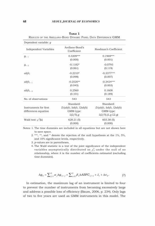
Table 1reSultS of the arellano-Bond dynamiC panel data differenCe Gmm
Dependent variable: g
Independent VariablesArellano-Bond’s
CoefficientRoodman’s Coefficient
gt – 1 0.3209***(0.000)
0.1969***(0.001)
gt – 2 -0.1182*(0.061)
-0.0793(0.119)
abfct -0.2210*(0.098)
-0.3377***(0.007)
abfct – 1 -0.2520**(0.045)
-0.3424***(0.003)
abfct – 2 0.2560(0.101)
0.1608(0.189)
No. of observations 543 543
Instruments for first differences equation
Standard:D.(abfc, labfc, l2abfc)
GMM-type:L(2/5).g
Standard:D.(abfc, labfc, l2abfc)
GMM-type:L(2/5).(L.g L2.g)
Wald test: χ 2(k) 628.21 (5)(0.000)
603.38 (5)(0.000)
Notes: 1. The time dummies are included in all equations but are not shown here to save space.
2. ***, **, and * denote the rejection of the null hypothesis at the 1%, 5%, and 10% significance levels, respectively.
3. p-values are in parentheses. 4. The Wald statistic is a test of the joint significance of the independent
variables asymptotically distributed as χ2k under the null of no
relationship, where k is the number of coefficients estimated (excluding time dummies).
69Macro econoMic effects of fiscal consolidation
estimation results of the growth rate function are shown in Table 1. The main result of estimation is that fiscal consolidation is not
expansionary but contractionary. GDP growth responds negatively to contemporaneous and lagged changes in action-based fiscal consolidation, indicating that fiscal consolidation typically reduces GDP growth. The results are statistically significant at the 10 per cent significance level at the least. Based on the above results, the idea of non-Keynesian effects that fiscal consolidation stimulates economic activity even in the short term cannot be supported empirically. The results are in line with those of Leigh et al. (2011) who used a policy action-based approach.
(b) Tests for the Validity of Over-Identifying RestrictionsThe Sargan–Hansen test for over-identifying restrictions has been
conducted in over-identified model estimated with instrumental variables techniques. The Sargan’s J-statistic has a null hypothesis that “the instruments as a group are exogenous.” This test is based on the idea that the residuals should be uncorrelated with the exogenous variables if the instruments are exogenous. In our estimation, the null hypothesis that over-identifying restrictions are valid is rejected. However, this result cannot be fully credible because the Sargan’s J-statistic is not powerful when many instrumental variables and heteroscedasticity in the error term exist (Arellano, and Bond 1991). When we employ Hansen’s J-statistic to address heteroscedasticity in the error term, the null hypothesis that over-identifying restrictions are valid is not rejected.
(c) Autocorrelation Test for the Differenced Error TermThe Arellano-Bond autocorrelation test is an important diagnostic
test of the residuals in the dynamic panel data estimation. With a null hypothesis of no autocorrelation, this test estimates the first- and second-order autocorrelation in the first-differenced residuals. By construction, the residuals of the Equation (7) Δvit should be serially correlated. However, if we assume serial independence in the original errors, the differenced residuals should not follow significant AR (2) process. If a significant AR (2) statistic exists, then the second lags of endogenous variables cannot be proper instruments for current values (Baum 2012).
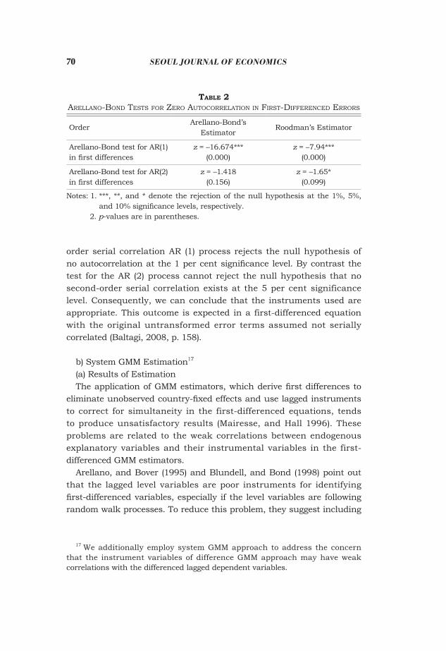
Table 2 shows the results of autocorrelation test. The test for first-
70 SEOUL JOURNAL OF ECONOMICS
order serial correlation AR (1) process rejects the null hypothesis of no autocorrelation at the 1 per cent significance level. By contrast the test for the AR (2) process cannot reject the null hypothesis that no second-order serial correlation exists at the 5 per cent significance level. Consequently, we can conclude that the instruments used are appropriate. This outcome is expected in a first-differenced equation with the original untransformed error terms assumed not serially correlated (Baltagi, 2008, p. 158).
b) System GMM Estimation17
(a) Results of EstimationThe application of GMM estimators, which derive first differences to
eliminate unobserved country-fixed effects and use lagged instruments to correct for simultaneity in the first-differenced equations, tends to produce unsatisfactory results (Mairesse, and Hall 1996). These problems are related to the weak correlations between endogenous explanatory variables and their instrumental variables in the first-differenced GMM estimators.
Arellano, and Bover (1995) and Blundell, and Bond (1998) point out that the lagged level variables are poor instruments for identifying first-differenced variables, especially if the level variables are following random walk processes. To reduce this problem, they suggest including
17 We additionally employ system GMM approach to address the concern that the instrument variables of difference GMM approach may have weak correlations with the differenced lagged dependent variables.
Table 2arellano-Bond teStS for Zero autoCorrelation in firSt-differenCed errorS
OrderArellano-Bond’s
EstimatorRoodman’s Estimator
Arellano-Bond test for AR(1) in first differences
z = –16.674***(0.000)
z = –7.94***(0.000)
Arellano-Bond test for AR(2) in first differences
z = –1.418(0.156)
z = –1.65*(0.099)
Notes: 1. ***, **, and * denote the rejection of the null hypothesis at the 1%, 5%, and 10% significance levels, respectively.
2. p-values are in parentheses.
71Macro econoMic effects of fiscal consolidation
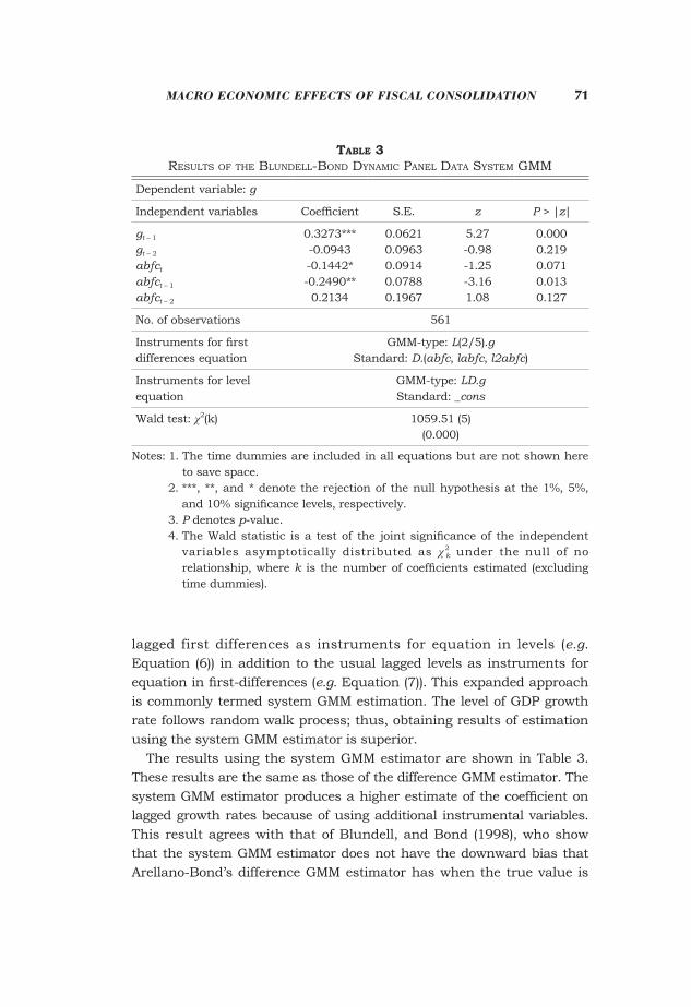
lagged first differences as instruments for equation in levels (e.g. Equation (6)) in addition to the usual lagged levels as instruments for equation in first-differences (e.g. Equation (7)). This expanded approach is commonly termed system GMM estimation. The level of GDP growth rate follows random walk process; thus, obtaining results of estimation using the system GMM estimator is superior.
The results using the system GMM estimator are shown in Table 3. These results are the same as those of the difference GMM estimator. The system GMM estimator produces a higher estimate of the coefficient on lagged growth rates because of using additional instrumental variables. This result agrees with that of Blundell, and Bond (1998), who show that the system GMM estimator does not have the downward bias that Arellano-Bond’s difference GMM estimator has when the true value is
Table 3reSultS of the Blundell-Bond dynamiC panel data SyStem Gmm
Dependent variable: g
Independent variables Coefficient S.E. z P > |z|
gt – 1
gt – 2
abfct
abfct – 1
abfct – 2
0.3273***-0.0943-0.1442*-0.2490**0.2134
0.06210.09630.09140.07880.1967
5.27-0.98-1.25-3.161.08
0.0000.2190.0710.0130.127
No. of observations 561
Instruments for first differences equation
GMM-type: L(2/5).gStandard: D.(abfc, labfc, l2abfc)
Instruments for level equation
GMM-type: LD.gStandard: _cons
Wald test: χ2(k) 1059.51 (5)(0.000)
Notes: 1. The time dummies are included in all equations but are not shown here to save space.
2. ***, **, and * denote the rejection of the null hypothesis at the 1%, 5%, and 10% significance levels, respectively.
3. P denotes p-value. 4. The Wald statistic is a test of the joint significance of the independent
variables asymptotically distributed as χ2k under the null of no
relationship, where k is the number of coefficients estimated (excluding time dummies).
72 SEOUL JOURNAL OF ECONOMICS
high.
(b) Tests for the Validity of Over-Identifying RestrictionsAccording to the Sargan’s J-statistic, the null hypothesis that over-
identifying restrictions are valid is rejected. However, as mentioned in the previous subsection, this result is not completely reliable because the Sargan’s J-statistic is not powerful when many instrumental variables and heteroscedasticity in the error term exist. When we employ Hansen’s J-statistic to address heteroscedasticity in the error term, the null hypothesis that over-identifying restrictions are valid is not rejected.
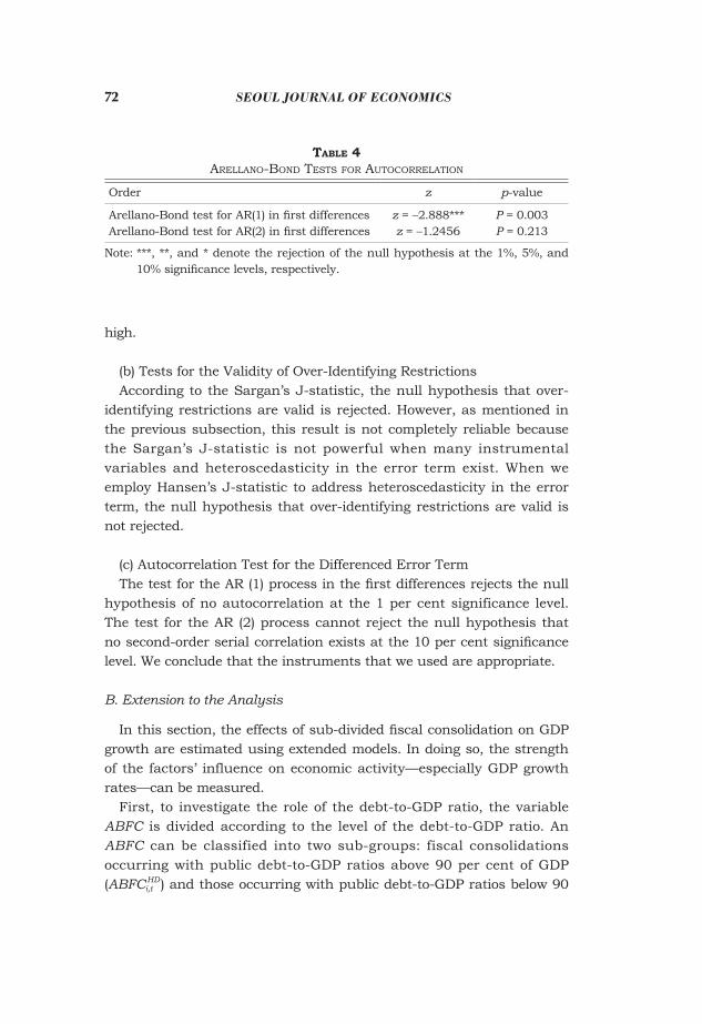
(c) Autocorrelation Test for the Differenced Error TermThe test for the AR (1) process in the first differences rejects the null
hypothesis of no autocorrelation at the 1 per cent significance level. The test for the AR (2) process cannot reject the null hypothesis that no second-order serial correlation exists at the 10 per cent significance level. We conclude that the instruments that we used are appropriate.
B. Extension to the Analysis
In this section, the effects of sub-divided fiscal consolidation on GDP growth are estimated using extended models. In doing so, the strength of the factors’ influence on economic activity—especially GDP growth rates—can be measured.
First, to investigate the role of the debt-to-GDP ratio, the variable ABFC is divided according to the level of the debt-to-GDP ratio. An ABFC can be classified into two sub-groups: fiscal consolidations occurring with public debt-to-GDP ratios above 90 per cent of GDP (ABFCi,t
HD ) and those occurring with public debt-to-GDP ratios below 90
Table 4arellano-Bond teStS for autoCorrelation
Order z p-value
Arellano-Bond test for AR(1) in first differencesArellano-Bond test for AR(2) in first differences
z = –2.888***z = –1.2456
P = 0.003P = 0.213
Note: ***, **, and * denote the rejection of the null hypothesis at the 1%, 5%, and 10% significance levels, respectively.
73Macro econoMic effects of fiscal consolidation
per cent of GDP (ABFCi,tLD ). The baseline model may be changed into the
following equation:
2 2, 1, ,1 0
22, ,0
.
HDit j i t j p i t pj p
HDp i t p i t itp
g g ABFC
ABFC v
α β
β γ µ
− −= =
−=
= +
+ + + +
∑ ∑∑
(8)
Table 5reSultS of Gmm eStimation ConSiderinG differenCe in deBt-to-Gdp ratioS
Dependent variable: g
Independent variables Coefficient S.E z P > |z|
gt – 1
gt – 2
abfc_hdt
abfc_hdt – 1
abfc_hdt – 2
abfc_ldt
abfc_ldt – 1
abfc_ldt – 2
0.1874***-0.0836-0.0457-0.4111*-0.3332
-0.3856***-0.3568***0.2828*
0.06290.05230.26180.22190.25490.14810.13760.1461
2.98-1.60-0.18-1.85-1.31-2.60-2.591.94
0.0030.1100.8610.0640.1910.0090.0090.053
No. of observations 544
Instruments for first differences equation
Standard:D.(abfc_hd, labfc_hd, l2abfc_hd abfc_ld, labfc_ld,
l2abfc_ld )GMM-type: L(2/5).(L.g L2.g)
Wald test: χ2(k) 668.29 (8)(0.000)
Arellano-Bond test for AR(1) in first differences
Z = –7.46 (p-value = 0.000)
Arellano-Bond test for AR(2) in first differences
Z = –1.26 (p-value = 0.207)
Notes: 1. The time dummies are included in all equations but are not shown here to save space.
2. ***, **, and * denote the rejection of the null hypothesis at the 1%, 5%, and 10% significance levels, respectively.
3. P denotes p-value. 4. The Wald statistic is a test of the joint significance of the independent
variables asymptotically distributed as χ2k under the null of no relation-
ship, where k is the number of coefficients estimated (excluding time dummies).
74 SEOUL JOURNAL OF ECONOMICS
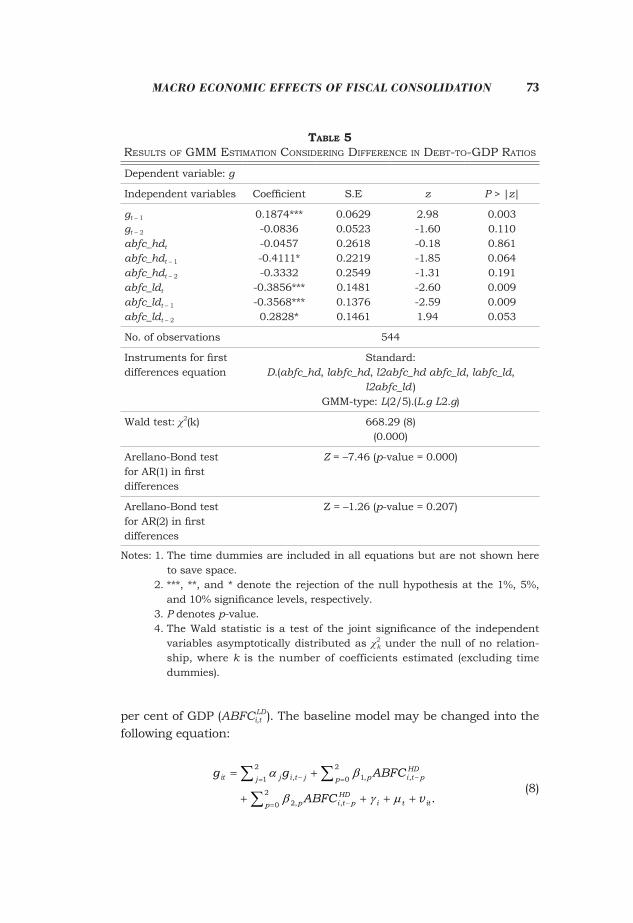
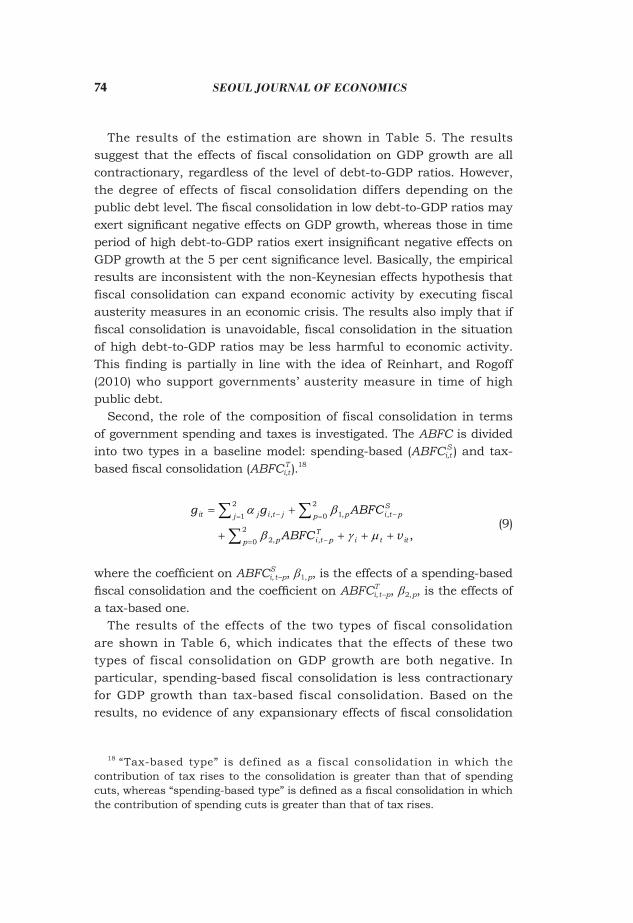
The results of the estimation are shown in Table 5. The results suggest that the effects of fiscal consolidation on GDP growth are all contractionary, regardless of the level of debt-to-GDP ratios. However, the degree of effects of fiscal consolidation differs depending on the public debt level. The fiscal consolidation in low debt-to-GDP ratios may exert significant negative effects on GDP growth, whereas those in time period of high debt-to-GDP ratios exert insignificant negative effects on GDP growth at the 5 per cent significance level. Basically, the empirical results are inconsistent with the non-Keynesian effects hypothesis that fiscal consolidation can expand economic activity by executing fiscal austerity measures in an economic crisis. The results also imply that if fiscal consolidation is unavoidable, fiscal consolidation in the situation of high debt-to-GDP ratios may be less harmful to economic activity. This finding is partially in line with the idea of Reinhart, and Rogoff (2010) who support governments’ austerity measure in time of high public debt.
Second, the role of the composition of fiscal consolidation in terms of government spending and taxes is investigated. The ABFC is divided into two types in a baseline model: spending-based (ABFCi,t
S ) and tax-based fiscal consolidation (ABFCi,t
T ).18
2 2, 1, ,1 0
22, ,0
,
Sit j i t j p i t pj p
Tp i t p i t itp
g g ABFC
ABFC v
α β
β γ µ
− −= =
−=
= +
+ + + +
∑ ∑∑
(9)
where the coefficient on ABFCi,S
t –p, β1, p, is the effects of a spending-based fiscal consolidation and the coefficient on ABFCi,
Tt –p, β2, p, is the effects of
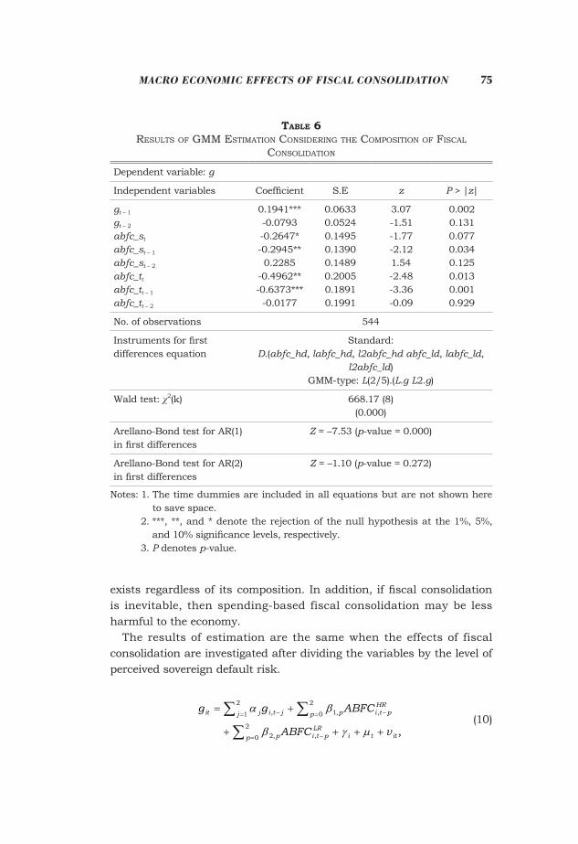
a tax-based one. The results of the effects of the two types of fiscal consolidation
are shown in Table 6, which indicates that the effects of these two types of fiscal consolidation on GDP growth are both negative. In particular, spending-based fiscal consolidation is less contractionary for GDP growth than tax-based fiscal consolidation. Based on the results, no evidence of any expansionary effects of fiscal consolidation
18 “Tax-based type” is defined as a fiscal consolidation in which the contribution of tax rises to the consolidation is greater than that of spending cuts, whereas “spending-based type” is defined as a fiscal consolidation in which the contribution of spending cuts is greater than that of tax rises.
75Macro econoMic effects of fiscal consolidation
exists regardless of its composition. In addition, if fiscal consolidation is inevitable, then spending-based fiscal consolidation may be less harmful to the economy.
The results of estimation are the same when the effects of fiscal consolidation are investigated after dividing the variables by the level of perceived sovereign default risk.
2 2
, 1, ,1 0
22, ,0
,
HRit j i t j p i t pj p
LRp i t p i t itp
g g ABFC
ABFC v
α β
β γ µ
− −= =
−=
= +
+ + + +
∑ ∑∑
(10)
Table 6reSultS of Gmm eStimation ConSiderinG the CompoSition of fiSCal
ConSolidation
Dependent variable: g
Independent variables Coefficient S.E z P > |z|
gt – 1
gt – 2
abfc_st
abfc_st – 1
abfc_st – 2
abfc_tt
abfc_tt – 1
abfc_tt – 2
0.1941***-0.0793-0.2647*-0.2945**0.2285
-0.4962**-0.6373***
-0.0177
0.06330.05240.14950.13900.14890.20050.18910.1991
3.07-1.51-1.77-2.121.54-2.48-3.36-0.09
0.0020.1310.0770.0340.1250.0130.0010.929
No. of observations 544
Instruments for first differences equation
Standard:D.(abfc_hd, labfc_hd, l2abfc_hd abfc_ld, labfc_ld,
l2abfc_ld)GMM-type: L(2/5).(L.g L2.g)
Wald test: χ2(k) 668.17 (8)(0.000)
Arellano-Bond test for AR(1) in first differences
Z = –7.53 (p-value = 0.000)
Arellano-Bond test for AR(2) in first differences
Z = –1.10 (p-value = 0.272)
Notes: 1. The time dummies are included in all equations but are not shown here to save space.
2. ***, **, and * denote the rejection of the null hypothesis at the 1%, 5%, and 10% significance levels, respectively.
3. P denotes p-value.
76 SEOUL JOURNAL OF ECONOMICS
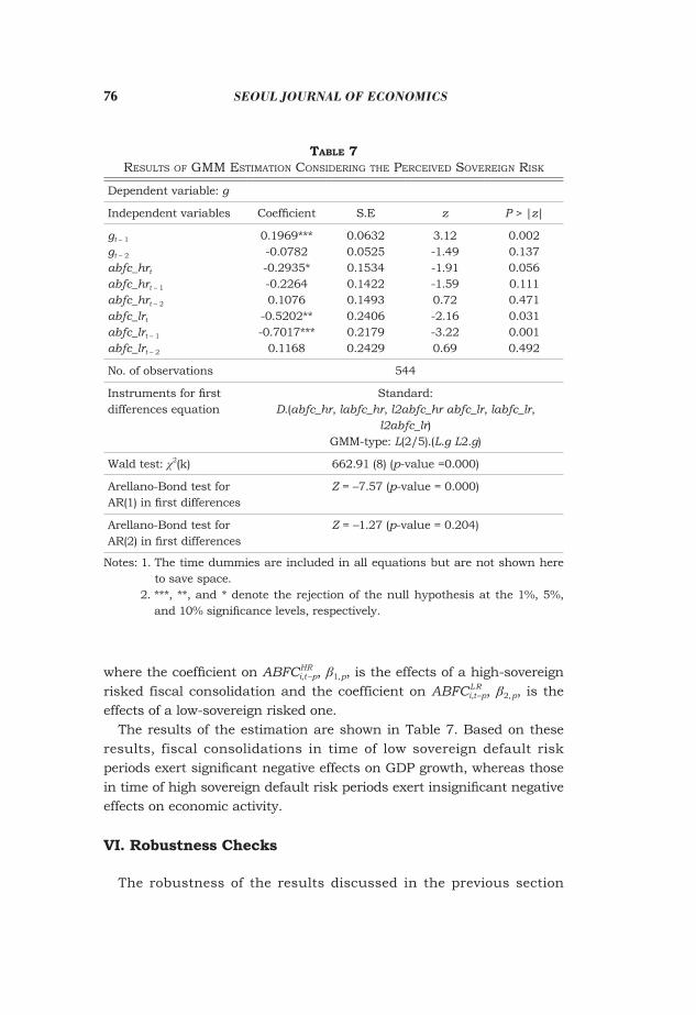
where the coefficient on ABFCi,HtR –p, β1, p, is the effects of a high-sovereign
risked fiscal consolidation and the coefficient on ABFCi,LtR –p, β2, p, is the
effects of a low-sovereign risked one. The results of the estimation are shown in Table 7. Based on these
results, fiscal consolidations in time of low sovereign default risk periods exert significant negative effects on GDP growth, whereas those in time of high sovereign default risk periods exert insignificant negative effects on economic activity.
VI. Robustness Checks
The robustness of the results discussed in the previous section
Table 7reSultS of Gmm eStimation ConSiderinG the perCeived SovereiGn riSK
Dependent variable: g
Independent variables Coefficient S.E z P > |z|
gt – 1
gt – 2
abfc_hrt
abfc_hrt – 1
abfc_hrt – 2
abfc_lrt
abfc_lrt – 1
abfc_lrt – 2
0.1969***-0.0782-0.2935*-0.22640.1076
-0.5202**-0.7017***
0.1168
0.06320.05250.15340.14220.14930.24060.21790.2429
3.12-1.49-1.91-1.590.72-2.16-3.220.69
0.0020.1370.0560.1110.4710.0310.0010.492
No. of observations 544
Instruments for first differences equation
Standard:D.(abfc_hr, labfc_hr, l2abfc_hr abfc_lr, labfc_lr,
l2abfc_lr)GMM-type: L(2/5).(L.g L2.g)
Wald test: χ2(k) 662.91 (8) (p-value =0.000)
Arellano-Bond test for AR(1) in first differences
Z = –7.57 (p-value = 0.000)
Arellano-Bond test for AR(2) in first differences
Z = –1.27 (p-value = 0.204)
Notes: 1. The time dummies are included in all equations but are not shown here to save space.
2. ***, **, and * denote the rejection of the null hypothesis at the 1%, 5%, and 10% significance levels, respectively.
77Macro econoMic effects of fiscal consolidation
depends on how independent variables have been controlled during estimation (Briotti 2005). In this section, we recheck whether fiscal consolidation exerts either non-Keynesian effects or contractionary effects on economic activity by performing several different tests.
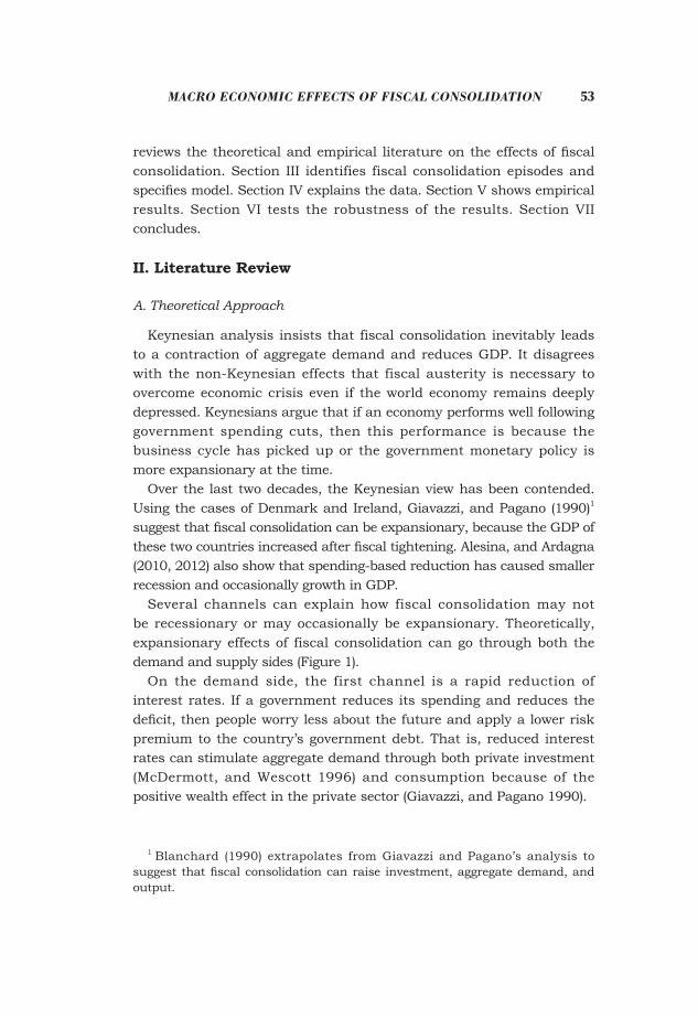
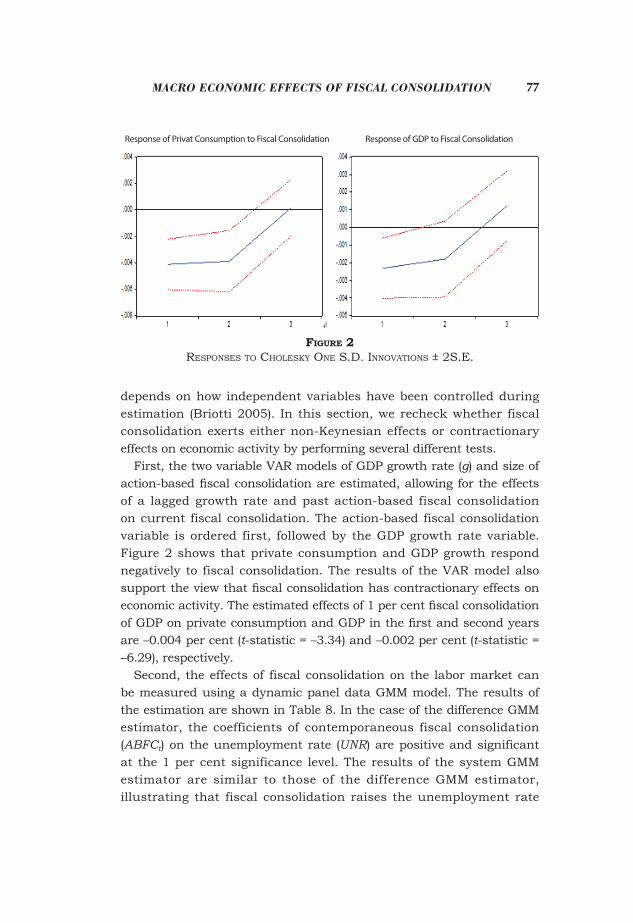
First, the two variable VAR models of GDP growth rate (g) and size of action-based fiscal consolidation are estimated, allowing for the effects of a lagged growth rate and past action-based fiscal consolidation on current fiscal consolidation. The action-based fiscal consolidation variable is ordered first, followed by the GDP growth rate variable. Figure 2 shows that private consumption and GDP growth respond negatively to fiscal consolidation. The results of the VAR model also support the view that fiscal consolidation has contractionary effects on economic activity. The estimated effects of 1 per cent fiscal consolidation of GDP on private consumption and GDP in the first and second years are –0.004 per cent (t-statistic = –3.34) and –0.002 per cent (t-statistic = –6.29), respectively.
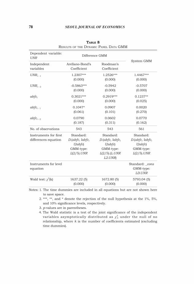
Second, the effects of fiscal consolidation on the labor market can be measured using a dynamic panel data GMM model. The results of the estimation are shown in Table 8. In the case of the difference GMM estimator, the coefficients of contemporaneous fiscal consolidation (ABFCt) on the unemployment rate (UNR) are positive and significant at the 1 per cent significance level. The results of the system GMM estimator are similar to those of the difference GMM estimator, illustrating that fiscal consolidation raises the unemployment rate
Figure 2reSponSeS to CholeSKy one S.d. innovationS ± 2S.e.
Response of Privat Consumption to Fiscal Consolidation Response of GDP to Fiscal Consolidation
78 SEOUL JOURNAL OF ECONOMICS
Table 8reSultS of the dynamiC panel data Gmm
Dependent variable: UNR
Difference GMM
System GMMIndependent variables
Arellano-Bond’s Coefficient
Roodman’s Coefficient
UNRt – 1 1.2307***(0.000)
1.2526***(0.000)
1.4467***(0.000)
UNRt – 2 -0.5863***(0.000)
-0.5942(0.000)
-0.5707(0.000)
abfct 0.3021***(0.000)
0.2919***(0.000)
0.1237**(0.025)
abfct – 1 0.1047*(0.061)
0.0907(0.101)
0.0020(0.270)
abfct – 2 0.0790(0.187)
0.0602(0.311)
0.0770(0.162)
No. of observations 543 543 561
Instruments for first differences equation
Standard:D.(abfc, labfc,
l2abfc)GMM-type:L(2/5).UNR
Standard:D.(abfc, labfc,
l2abfc)GMM-type:
L(2/5).(L.UNR L2.UNR)
Standard:D.(abfc, labfc,
l2abfc)GMM-type:L(2/5).UNR
Instruments for level equation
Standard: _consGMM-type:
LD.UNR
Wald test: χ2(k) 1637.22 (5)(0.000)
1672.80 (5)(0.000)
5793.04 (5)(0.000)
Notes: 1. The time dummies are included in all equations but are not shown here to save space.
2. ***, **, and * denote the rejection of the null hypothesis at the 1%, 5%, and 10% significance levels, respectively.
3. p-values are in parentheses. 4. The Wald statistic is a test of the joint significance of the independent
variables asymptotically distributed as χ2k under the null of no
relationship, where k is the number of coefficients estimated (excluding time dummies).
79Macro econoMic effects of fiscal consolidation
Table 9reSultS of the arellano-Bond differenCe Gmm with Control variaBleS
Alternatives
Independent variables
Coefficient
(1) (2) (3) (4) (5)
gt – 1 0.1969***(0.001)
0.2024***(0.001)
0.2051***(0.001)
0.1420**(0.022)
0.2934***(0.000)
gt – 2 -0.0793(0.119)
-0.1049*(0.054)
-0.0885*(0.085)
-0.1108**(0.030)
-0.1522**(0.027)
abfct -0.3377***(0.007)
-0.3344***(0.007)
-0.3323***(0.008)
-0.2724**(0.026)
-0.3437***(0.003)
abfct – 1 -0.3424***(0.003)
-0.3408***(0.003)
-0.3270**(0.005)
-0.2752**(0.016)
-0.1845(0.116)
abfct – 2 0.1608(0.189)
0.1454(0.235)
0.1643(0.181)
0.1856(0.118)
0.1587(0.191)
IRL - -0.0018**(0.015)
- - -
EXCHEB - - -0.0001**(0.024)
- -
UNR - - - -0.0020***(0.007)
-
IIR - - - 0.0004(0.295)
No. of observations 543 541 543 543 479
Wald test: χ2(k) 603.38 (5) 693.17 (6) 684.51 (6) 736.20 (6) 853.53 (6)
Notes: 1. The time dummies are included in all equations but are not shown here to save space.
2. ***, **, and * denote the rejection of the null hypothesis at the 1%, 5%, and 10% significance levels, respectively.
3. p-values are in parentheses. 4. The Wald statistic is a test of the joint significance of the independent
variables asymptotically distributed as χ2k under the null of no
relationship, where k is the number of coefficients estimated (excluding time dummies).
80 SEOUL JOURNAL OF ECONOMICS
significantly. Moreover, the results support our empirical finding that fiscal consolidation exerts negative effects on economic activity.
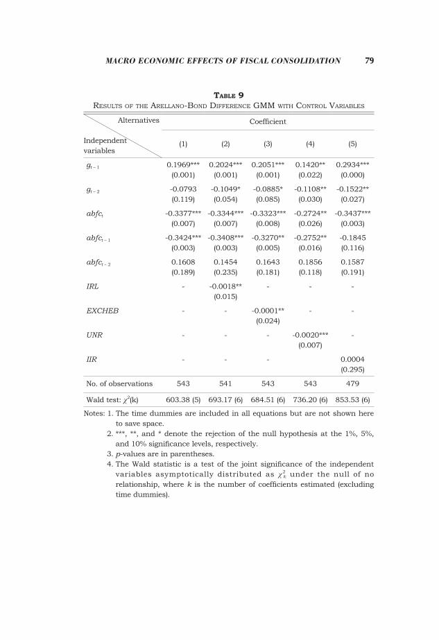
Third, several control variables are added to address the possibility that the baseline equation omits variables affecting economic activity, which are correlated with fiscal consolidation. The omitted variables can be a number of additional non-policy factors, such as long-term interest rates (IRL), nominal effective exchange rates (EXCHEB),19 UNR, and perceived sovereign default risk. As for the sovereign default risk, the IIR index20 is used as a proxy measure of the perceived sovereign default risk, following Reinhart, Rogoff, and Savastano (2003) and Eichengreen, and Mody (2004). The results of the estimation are shown in Table 9. The results are also similar to those of the baseline equation.21 The changes in interest, exchange, and unemployment rates help to cushion or mitigate the negative effect of fiscal consolidation on economic growth.
VII. Conclusion
This paper has investigated whether expansionary fiscal consolidation exists using dynamic panel data analysis with GMM estimation. Although the non-Keynesian effects of fiscal consolidation is theoretically reasonable and attractive, obtaining empirical evidence is challenging because of the difficulty of gaining credibility for the policy (Prammer 2004). A reform process on the basis of fiscal consolidation alone, in the middle of an economic crisis, can be exposed to the risk of self-defeating. Fiscal consolidation in an economic recession may lead domestic demand to fall into line with consumers’ rising concerns about job security and disposable incomes, thus reducing national tax revenues.
According to the estimates of dynamic panel data analysis with GMM estimation, fiscal consolidation is not expansionary in terms of GDP growth
19 A rise of nominal effective exchange rates indicates an appreciation of the Korean won.
20 The ratings are based on assessments of sovereign risk by private sector analysts. They rate each country on a scale of 0 to 100, with a rating of 100 assigned to the lowest perceived sovereign default risk probability.
21 The results are the same when two lags of the additional control variable are implemented in the equation.
81Macro econoMic effects of fiscal consolidation
but rather contractionary. Unlike the ideas of non-Keynesian effects, our empirical estimates show that fiscal consolidation reduces the GDP growth rate significantly. The view that fiscal consolidation may stimulate the economy in the short term cannot be supported. This outcome is in line with the suggestion of the IMF (2010).
Both the Arellano-Bond difference GMM estimation and Blundell-Bond system GMM estimation show that fiscal consolidation exerts significant negative effects on economic growth. The results are similar when the baseline model is extended by considering several factors.
According to the results produced by extension models, fiscal consolidation during high debt-to-GDP ratios exerts less negative effects on economic growth than that during low debt-to-GDP ratios. In addition, fiscal consolidation based on the spending cuts is less damaging to the economy than that based on tax hikes. Moreover, fiscal consolidation when the sovereign default risk is high is less costly to economic growth than that when the sovereign default risk is low.
(Received 3 May 2016; Revised 21 July 2016; Accepted 18 August 2016)
Appendix
A. Various Ways of Measuring CAPB
The CAPB is calculated by deriving the actual primary balance (non-interest government revenue minus non-interest government spending) and subtracting the estimated effect of business cycle fluctuations on fiscal accounts (IMF 2010). Cyclical adjustment of fiscal variables uses three approaches.
A.1. Hodrick–Prescott (HP) filter (Hodrick, and Prescott 1980; Kydland, and Prescott 1990)
This smoothing approach computes the cyclically adjusted measure (yt
*) of a variable (yt) by the following expression:
λ −+ −= =
− + − − −∑ ∑ 1* 2 * * * * 21 11 2
Min ( ) (( ) ( )) .T Tt t t t t tt t
y y y y y y
The crucial point in the application of the HP filter is the choice of the weighting factor, determining the degree of smoothness. In the case of annual data, λ is set to 100.
82 SEOUL JOURNAL OF ECONOMICS
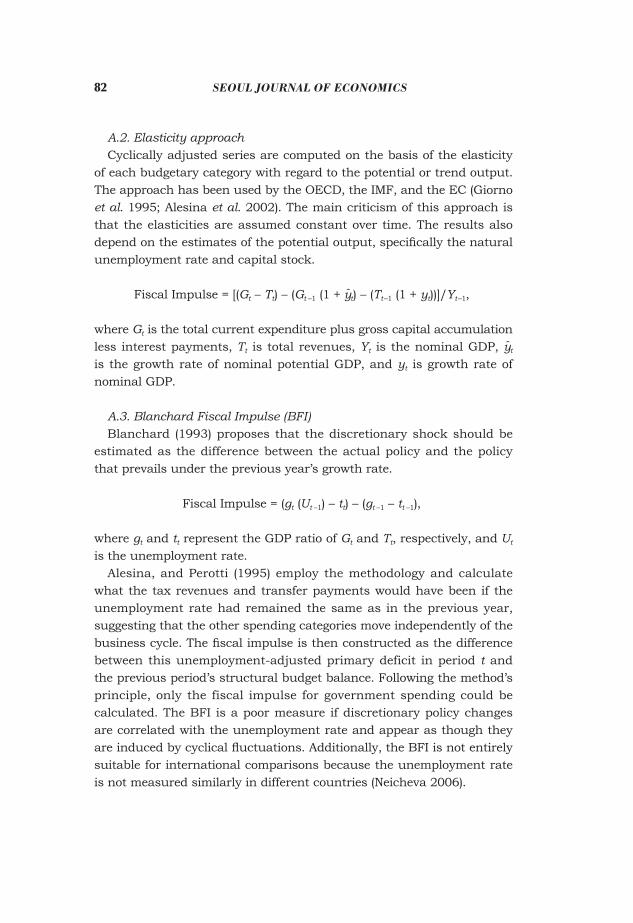
A.2. Elasticity approach Cyclically adjusted series are computed on the basis of the elasticity
of each budgetary category with regard to the potential or trend output. The approach has been used by the OECD, the IMF, and the EC (Giorno et al. 1995; Alesina et al. 2002). The main criticism of this approach is that the elasticities are assumed constant over time. The results also depend on the estimates of the potential output, specifically the natural unemployment rate and capital stock.
Fiscal Impulse = [(Gt – Tt) – (Gt –1 (1 + yt) – (Tt –1 (1 + yt))]/Yt –1,
where Gt is the total current expenditure plus gross capital accumulation less interest payments, Tt is total revenues, Yt is the nominal GDP, yt is the growth rate of nominal potential GDP, and yt is growth rate of nominal GDP.
A.3. Blanchard Fiscal Impulse (BFI) Blanchard (1993) proposes that the discretionary shock should be
estimated as the difference between the actual policy and the policy that prevails under the previous year’s growth rate.
Fiscal Impulse = (gt (Ut –1) – tt) – (gt –1 – tt –1),
where gt and tt represent the GDP ratio of Gt and Tt, respectively, and Ut is the unemployment rate.
Alesina, and Perotti (1995) employ the methodology and calculate what the tax revenues and transfer payments would have been if the unemployment rate had remained the same as in the previous year, suggesting that the other spending categories move independently of the business cycle. The fiscal impulse is then constructed as the difference between this unemployment-adjusted primary deficit in period t and the previous period’s structural budget balance. Following the method’s principle, only the fiscal impulse for government spending could be calculated. The BFI is a poor measure if discretionary policy changes are correlated with the unemployment rate and appear as though they are induced by cyclical fluctuations. Additionally, the BFI is not entirely suitable for international comparisons because the unemployment rate is not measured similarly in different countries (Neicheva 2006).
83Macro econoMic effects of fiscal consolidation
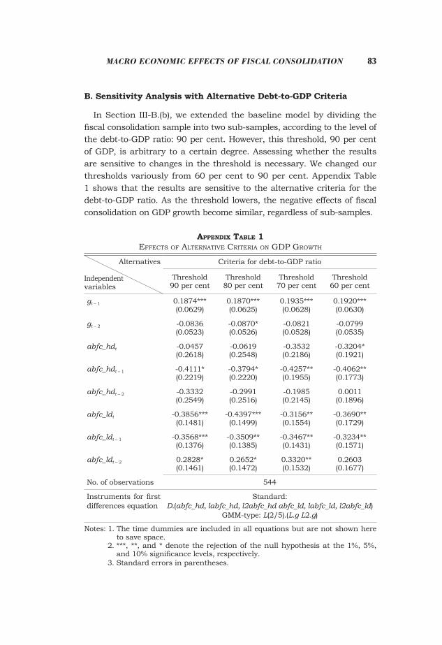
B. Sensitivity Analysis with Alternative Debt-to-GDP Criteria
In Section III-B.(b), we extended the baseline model by dividing the fiscal consolidation sample into two sub-samples, according to the level of the debt-to-GDP ratio: 90 per cent. However, this threshold, 90 per cent of GDP, is arbitrary to a certain degree. Assessing whether the results are sensitive to changes in the threshold is necessary. We changed our thresholds variously from 60 per cent to 90 per cent. Appendix Table 1 shows that the results are sensitive to the alternative criteria for the debt-to-GDP ratio. As the threshold lowers, the negative effects of fiscal consolidation on GDP growth become similar, regardless of sub-samples.
appendix Table 1effeCtS of alternative Criteria on Gdp Growth
Alternatives
Independent variables
Criteria for debt-to-GDP ratio
Threshold90 per cent
Threshold80 per cent
Threshold70 per cent
Threshold60 per cent
gt – 1 0.1874***(0.0629)
0.1870***(0.0625)
0.1935***(0.0628)
0.1920***(0.0630)
gt – 2 -0.0836(0.0523)
-0.0870*(0.0526)
-0.0821(0.0528)
-0.0799(0.0535)
abfc_hdt -0.0457(0.2618)
-0.0619(0.2548)
-0.3532(0.2186)
-0.3204*(0.1921)
abfc_hdt – 1 -0.4111*(0.2219)
-0.3794*(0.2220)
-0.4257**(0.1955)
-0.4062**(0.1773)
abfc_hdt – 2 -0.3332(0.2549)
-0.2991(0.2516)
-0.1985(0.2145)
0.0011(0.1896)
abfc_ldt -0.3856***(0.1481)
-0.4397***(0.1499)
-0.3156**(0.1554)
-0.3690**(0.1729)
abfc_ldt – 1 -0.3568***(0.1376)
-0.3509**(0.1385)
-0.3467**(0.1431)
-0.3234**(0.1571)
abfc_ldt – 2 0.2828*(0.1461)
0.2652*(0.1472)
0.3320**(0.1532)
0.2603(0.1677)
No. of observations 544
Instruments for first differences equation
Standard:D.(abfc_hd, labfc_hd, l2abfc_hd abfc_ld, labfc_ld, l2abfc_ld)
GMM-type: L(2/5).(L.g L2.g)
Notes: 1. The time dummies are included in all equations but are not shown here to save space.
2. ***, **, and * denote the rejection of the null hypothesis at the 1%, 5%, and 10% significance levels, respectively.
3. Standard errors in parentheses.
84 SEOUL JOURNAL OF ECONOMICS
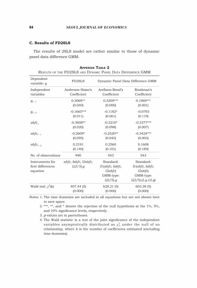
C. Results of FD2SLS
The results of 2SLS model are rather similar to those of dynamic panel data difference GMM.
appendix Table 2reSultS of the fd2SlS and dynamiC panel data differenCe Gmm
Dependent variable: g
FD2SLS Dynamic Panel Data Difference GMM
Independent variables
Anderson-Hsiao’s Coefficient
Arellano-Bond’s Coefficient
Roodman’s Coefficient
gt – 1 0.3069**(0.040)
0.3209***(0.000)
0.1969***(0.001)
gt – 2 -0.1665***(0.011)
-0.1182*(0.061)
-0.0793(0.119)
abfc_ -0.3608**(0.020)
-0.2210*(0.098)
-0.3377***(0.007)
abfct – 1 -0.2609*(0.095)
-0.2520**(0.045)
-0.3424***(0.003)
abfct – 2 0.2191(0.140)
0.2560(0.101)
0.1608(0.189)
No. of observations 490 543 543
Instruments for first differences equation
abfc, labfc, l2abfc, L(2/5).g
Standard:D.(abfc, labfc,
l2abfc)GMM-type:
L(2/5).g
Standard:D.(abfc, labfc,
l2abfc)GMM-type:
L(2/5).(L.g L2.g)
Wald test: χ2(k) 407.44 (5)(0.000)
628.21 (5)(0.000)
603.38 (5)(0.000)
Notes: 1. The time dummies are included in all equations but are not shown here to save space.
2. ***, **, and * denote the rejection of the null hypothesis at the 1%, 5%, and 10% significance levels, respectively.
3. p-values are in parentheses. 4. The Wald statistic is a test of the joint significance of the independent
variables asymptotically distributed as χ2k under the null of no
relationship, where k is the number of coefficients estimated (excluding time dummies).
85Macro econoMic effects of fiscal consolidation
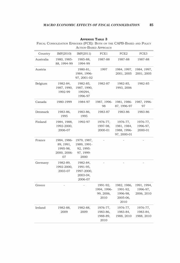
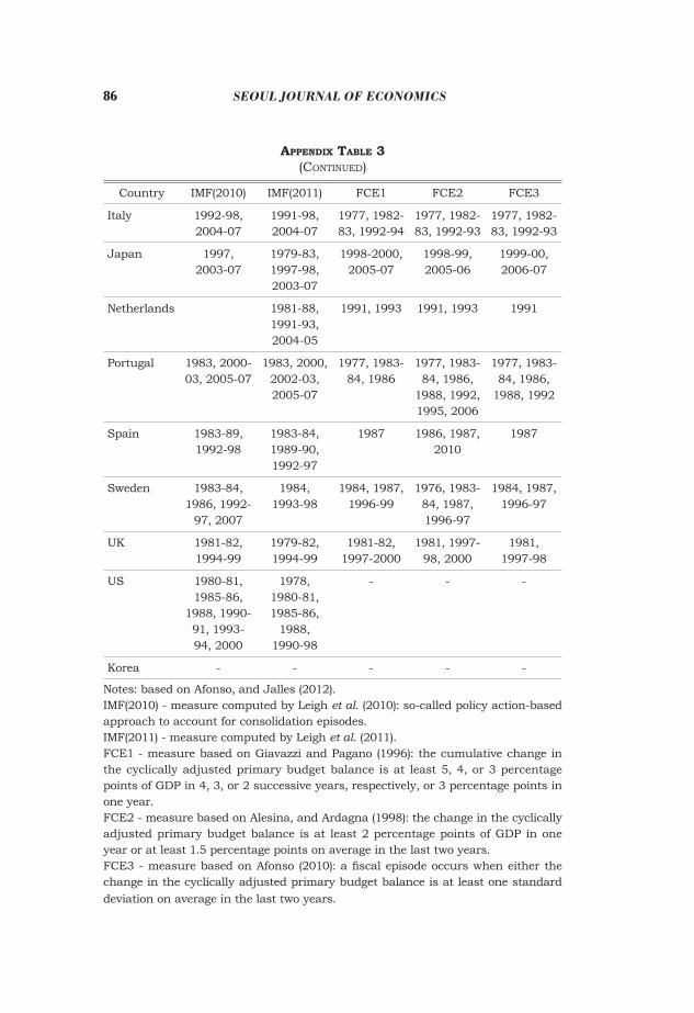
appendix Table 3fiSCal ConSolidation epiSodeS (fCe): Both on the CapB-BaSed and poliCy
aCtion-BaSed approaCh
Country IMF(2010) IMF(2011) FCE1 FCE2 FCE3
Australia 1980, 1985-88, 1994-99
1985-88, 1994-99
1987-88 1987-88 1987-88
Austria 1980-81, 1984, 1996-97, 2001-02
1997 1984, 1997, 2001, 2005
1984, 1997, 2001, 2005
Belgium 1982-84, 1987, 1990,
1992-99
1982-85, 1987, 1990,
199294, 1996-97
1982-87 1982-85, 1993, 2006
1982-85
Canada 1980-1999 1984-97 1987, 1996-98
1981, 1986-87, 1996-97
1987, 1996-97
Denmark 1983-86, 1995
1983-86, 1995
1983-87 1983-86 1983-86
Finland 1984, 1988, 1992-2000,
2006-07
1992-97 1976-77, 1997-98, 2000-01
1976-77, 1981, 1984, 1988, 1996-97, 2000-01
1976-77, 1996-97, 2000-01
France 1984, 1986-89, 1991, 1995-98,
2000, 2006-07
1979, 1987, 1989, 1991-92, 1995-97, 1999-
2000
- - -
Germany 1982-89, 1992-2000,
2003-07
1982-84, 1991-95,
1997-2000, 2003-04, 2006-07
- - -
Greece - - 1991-92, 1994, 1996-99, 2006,
2010
1982, 1986, 1991-92, 1996-98, 2005-06,
2010
1991, 1994, 1996-97,
2006, 2010
Ireland 1982-88, 2009
1982-88, 2009
1976-77, 1983-86, 1988-89,
2010
1976-77, 1983-84,
1988, 2010
1976-77, 1983-84,
1988, 2010
86 SEOUL JOURNAL OF ECONOMICS
Country IMF(2010) IMF(2011) FCE1 FCE2 FCE3
Italy 1992-98, 2004-07
1991-98, 2004-07
1977, 1982-83, 1992-94
1977, 1982-83, 1992-93
1977, 1982-83, 1992-93
Japan 1997, 2003-07
1979-83, 1997-98, 2003-07
1998-2000, 2005-07
1998-99, 2005-06
1999-00, 2006-07
Netherlands 1981-88, 1991-93, 2004-05
1991, 1993 1991, 1993 1991
Portugal 1983, 2000-03, 2005-07
1983, 2000, 2002-03, 2005-07
1977, 1983-84, 1986
1977, 1983-84, 1986,
1988, 1992, 1995, 2006
1977, 1983-84, 1986,
1988, 1992
Spain 1983-89, 1992-98
1983-84, 1989-90, 1992-97
1987 1986, 1987, 2010
1987
Sweden 1983-84, 1986, 1992-
97, 2007
1984, 1993-98
1984, 1987, 1996-99
1976, 1983-84, 1987, 1996-97
1984, 1987, 1996-97
UK 1981-82, 1994-99
1979-82, 1994-99
1981-82, 1997-2000
1981, 1997-98, 2000
1981, 1997-98
US 1980-81, 1985-86,
1988, 1990-91, 1993-94, 2000
1978, 1980-81, 1985-86,
1988, 1990-98
- - -
Korea - - - - -
Notes: based on Afonso, and Jalles (2012).IMF(2010) - measure computed by Leigh et al. (2010): so-called policy action-based approach to account for consolidation episodes.IMF(2011) - measure computed by Leigh et al. (2011).FCE1 - measure based on Giavazzi and Pagano (1996): the cumulative change in the cyclically adjusted primary budget balance is at least 5, 4, or 3 percentage points of GDP in 4, 3, or 2 successive years, respectively, or 3 percentage points in one year. FCE2 - measure based on Alesina, and Ardagna (1998): the change in the cyclically adjusted primary budget balance is at least 2 percentage points of GDP in one year or at least 1.5 percentage points on average in the last two years.FCE3 - measure based on Afonso (2010): a fiscal episode occurs when either the change in the cyclically adjusted primary budget balance is at least one standard deviation on average in the last two years.
appendix Table 3(Continued)
87Macro econoMic effects of fiscal consolidation
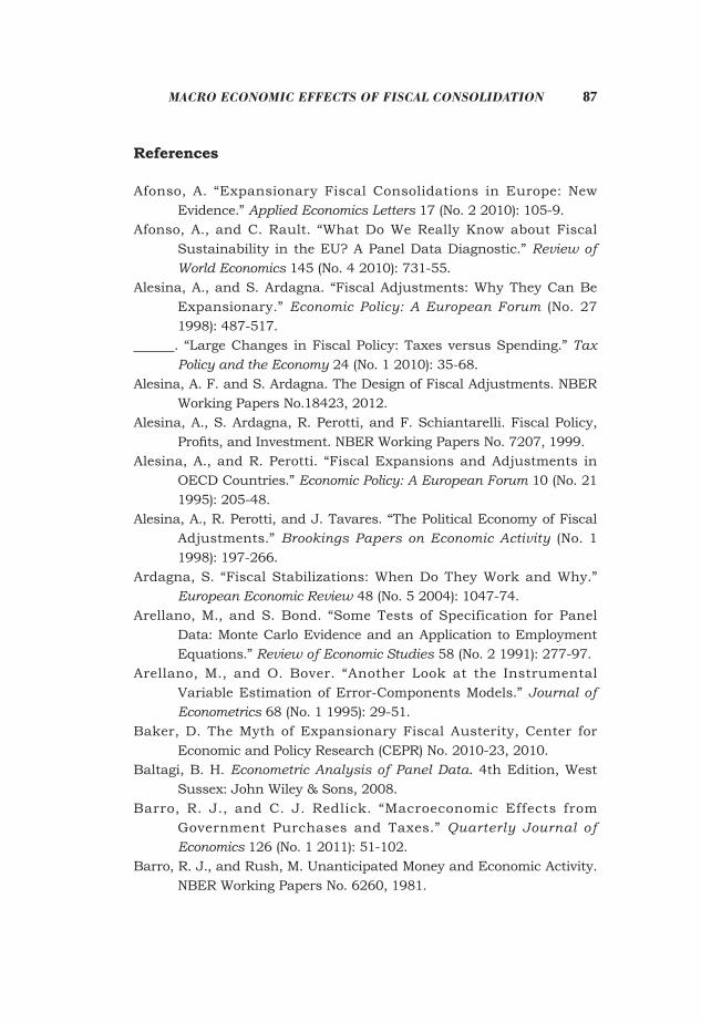
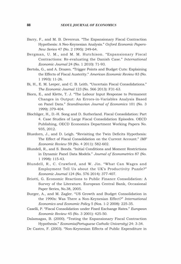
References
Afonso, A. “Expansionary Fiscal Consolidations in Europe: New Evidence.” Applied Economics Letters 17 (No. 2 2010): 105-9.
Afonso, A., and C. Rault. “What Do We Really Know about Fiscal Sustainability in the EU? A Panel Data Diagnostic.” Review of World Economics 145 (No. 4 2010): 731-55.
Alesina, A., and S. Ardagna. “Fiscal Adjustments: Why They Can Be Expansionary.” Economic Policy: A European Forum (No. 27 1998): 487-517.
. “Large Changes in Fiscal Policy: Taxes versus Spending.” Tax Policy and the Economy 24 (No. 1 2010): 35-68.
Alesina, A. F. and S. Ardagna. The Design of Fiscal Adjustments. NBER Working Papers No.18423, 2012.
Alesina, A., S. Ardagna, R. Perotti, and F. Schiantarelli. Fiscal Policy, Profits, and Investment. NBER Working Papers No. 7207, 1999.
Alesina, A., and R. Perotti. “Fiscal Expansions and Adjustments in OECD Countries.” Economic Policy: A European Forum 10 (No. 21 1995): 205-48.
Alesina, A., R. Perotti, and J. Tavares. “The Political Economy of Fiscal Adjustments.” Brookings Papers on Economic Activity (No. 1 1998): 197-266.
Ardagna, S. “Fiscal Stabilizations: When Do They Work and Why.” European Economic Review 48 (No. 5 2004): 1047-74.
Arellano, M., and S. Bond. “Some Tests of Specification for Panel Data: Monte Carlo Evidence and an Application to Employment Equations.” Review of Economic Studies 58 (No. 2 1991): 277-97.
Arellano, M., and O. Bover. “Another Look at the Instrumental Variable Estimation of Error-Components Models.” Journal of Econometrics 68 (No. 1 1995): 29-51.
Baker, D. The Myth of Expansionary Fiscal Austerity, Center for Economic and Policy Research (CEPR) No. 2010-23, 2010.
Baltagi, B. H. Econometric Analysis of Panel Data. 4th Edition, West Sussex: John Wiley & Sons, 2008.
Barro, R. J., and C. J. Redlick. “Macroeconomic Effects from Government Purchases and Taxes.” Quarterly Journal of Economics 126 (No. 1 2011): 51-102.
Barro, R. J., and Rush, M. Unanticipated Money and Economic Activity. NBER Working Papers No. 6260, 1981.
88 SEOUL JOURNAL OF ECONOMICS
Barry, F., and M. B. Devereux. “The Expansionary Fiscal Contraction Hypothesis: A Neo-Keynesian Analysis.” Oxford Economic Papers-New Series 47 (No. 2 1995): 249-64.
Bergman, U. M., and M. M. Hutchison. “Expansionary Fiscal Contractions: Re-evaluating the Danish Case.” International Economic Journal 24 (No. 1 2010): 71-93.
Bertola, G., and A. Drazen. “Trigger Points and Budget Cuts: Explaining the Effects of Fiscal Austerity.” American Economic Review 83 (No. 1 1993): 11-26.
Bi, H., E. M. Leeper, and C. B. Leith. “Uncertain Fiscal Consolidations.” The Economic Journal 123 (No. 566 2013): F31-63.
Biorn, E., and Klette, T. J. “The Labour Input Response to Permanent Changes in Output: An Errors-in-Variables Analysis Based on Panel Data.” Scandinavian Journal of Economics 101 (No. 3 1999): 379-404.
Blochliger, H., D.-H. Song and D. Sutherland. Fiscal Consolidation: Part 4. Case Studies of Large Fiscal Consolidation Episodes. OECD Publishing, OECD Economics Department Working Papers No. 935, 2012.
Bluedorn, J., and D. Leigh. “Revisiting the Twin Deficits Hypothesis: The Effect of Fiscal Consolidation on the Current Account.” IMF Economic Review 59 (No. 4 2011): 582-602.
Blundell, R., and S. Bonds. “Initial Conditions and Moment Restrictions in Dynamic Panel Data Models.” Journal of Econometrics 87 (No. 1 1998): 115-43.
Blundell, R., C. Crawford, and W. Jin. “What Can Wages and Employment Tell Us about the UK’s Productivity Puzzle?” Economic Journal 124 (No. 576 2014): 377-407.
Briotti, G. Economic Reactions to Public Finance Consolidation: A Survey of the Literature. European Central Bank, Occasional Paper Series, No.38, 2005.
Burger, A., and M. Zagler. “US Growth and Budget Consolidation in the 1990s: Was There a Non-Keynesian Effect?” International Economics and Economic Policy 5 (Nos. 1-2 2008): 225-35.
Caselli, P. “Fiscal Consolidation under Fixed Exchange Rates.” European Economic Review 45 (No. 3 2001): 425-50.
Dalamagas, B. (2000). “Testing the Expansionary Fiscal Contraction Hypothesis.” Economia(Portuguese Catholic University) 24: 3-34.
De Castro, F. (2003). “Non-Keynesian Effects of Public Expenditure in
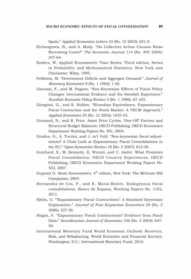
89Macro econoMic effects of fiscal consolidation
Spain.” Applied Economics Letters 10 (No. 10 2003): 651-5.Eichengreen, B., and A. Mody. “Do Collective Action Clauses Raise
Borrowing Costs?” The Economic Journal 114 (No. 495 2004): 247-64.
Enders, W. Applied Econometric Time Series. Third edition, Series in Probability and Mathematical Statistics. New York and Chichester: Wiley, 1995.
Feldstein, M. “Government Deficits and Aggregate Demand.” Journal of Monetary Economics 9 (No. 1 1982): 1-20.
Giavazzi, F., and M. Pagano. “Non-Keynesian Effects of Fiscal Policy Changes: International Evidence and the Swedish Experience.” Swedish Economic Policy Review 3 (No. 1 1996): 67-103.
Giorgioni, G., and K. Holden. “Ricardian Equivalence, Expansionary Fiscal Contraction and the Stock Market: A VECM Approach.” Applied Economics 35 (No. 12 2003): 1435-43.
Girouard, N., and R. Price. Asset Price Cycles, ‘One-Off’ Factors and Structural Budget Balances. OECD Publishing, OECD Economics Department Working Papers No. 391, 2004.
Giudice, G., A. Turrini, and J. in’t Veld. “Non-keynesian fiscal adjust-ments? A Close Look at Expansionary Fiscal Consolidations in the EU.” Open Economies Review 18 (No. 5 2007): 613-30.
Guichard, S., M. Kennedy, E. Wurzel, and C. Andre. What Promotes Fiscal Consolidation: OECD Country Experiences. OECD Publishing, OECD Economics Department Working Papers No. 553, 2007.
Gujarati D. Basic Econometrics. 4th edition, New York: The McGraw–Hill Companies, 2004.
Hernandez de Cos, P., and E. Moral-Benito. Endogenous fiscal consolidations. Banco de Espana, Working Papers No. 1102, 2011.
Hjelm, G. “’Expansionary Fiscal Contractions’: A Standard Keynesian Explanation.” Journal of Post Keynesian Economics 29 (No. 2 2006): 327-58.
Hogan, V. “Expansionary Fiscal Contractions? Evidence from Panel Data.” Scandinavian Journal of Economics 106 (No. 4 2004): 647-59.
International Monetary Fund World Economic Outlook: Recovery, Risk, and Rebalancing. World Economic and Financial Surveys. Washington, D.C.: International Monetary Fund, 2010.
90 SEOUL JOURNAL OF ECONOMICS
Kim, Soyoung. “Monetary Instrument Problem Revisited: The Role of Fiscal Policy.” Seoul Journal of Economics 24 (No. 4 2011): 525-50.
Krugman, P. “Myths of Austerity.” New York Times Op-Ed Column, July 2, 2010.
Leigh, D., A. Pescatori, and J. Guajardo. Expansionary Austerity New International Evidence. International Monetary Fund, IMF Working Papers No. 11/158, 2011.
Leigh, D., A. Pescatori, J. Guajardo, and P. Devries. A New Action-based Dataset of Fiscal Consolidation. International Monetary Fund, IMF Working Papers No. 11/128, 2011.
Mairesse, J., and B. H. Hall. Estimating the Productivity of Research and Development: An Exploration of GMM Methods Using Data on French & United States Manufacturing Firms. NBER Working Papers No. 5501, 1996.
McDermott, C. J., and R. F. Wescott. “An Empirical Analysis of Fiscal Adjustments.” International Monetary Fund Staff Papers 43 (No. 4 1996): 725-53.
Miller, S. M., and F. S. Russek. “The Relationship between Large Fiscal Adjustments and Short-Term Output Growth under Alternative Fiscal Policy Regimes.” Contemporary Economic Policy 21 (No. 1 2003): 41-58.
Molnar, M. Fiscal Consolidation: Part 5. What Factors Determine the Success of Consolidation Efforts?, OECD Publishing, OECD Eco-nomics Department Working Papers No. 936, 2012.
Neicheva, M. “Non-Keynesian Effects of Government Expenditure on Output in Bulgaria: An HP Filter Approach.” Post-Communist Economies 18 (No. 1 2006): 1-12.
Perotti, R. “In Search of the Transmission Mechanism of Fiscal Policy.” NBER Macroeconomics Annual 22 (2007): 169-249.
Perotti, R. The ‘Austerity Myth’: Gain without Pain?. CEPR Discussion Papers No. 8658, 2011.
Prammer, D. “Expansionary Fiscal Consolidations? An Appraisal of the Literature on Non-Keynesian Effects of Fiscal Policy and a Case Study for Austria.” Monetary Policy and the Economy (2004): 34-52.
Ramey, V. A. “Identifying Government Spending Shocks: It’s All in the Timing.” Quarterly Journal of Economics 126 (No. 1 2011): 1-50.
Ramey, V. A., and M. D. Shapiro. “Costly Capital Reallocation and the
91Macro econoMic effects of fiscal consolidation
Effects of Government Spending.” Carnegie-Rochester Conference Series on Public Policy 48 (1998): 145-94.
Reinhart, C. M., and K. S. Rogoff. “Growth in a Time of Debt.” American Economic Review 100 (No. 2 2010): 573-8.
Reinhart, C. M., K. S. Rogoff, and M. A. Savastano. “Debt Intolerance.” Brookings Papers on Economic Activity 34 (No. 1 2003): 1-74.
Romer, C. D., and D. H. Romer. “Credit Channel or Credit Actions? An Interpretation of the Postwar Transmission Mechanism.” Chang-ing Capital Markets: Implications for Monetary Policy (1993): 71-116.
Romer, C. D., and D. H. Romer. “The Macroeconomic Effects of Tax Changes: Based on a New Measure of Fiscal Shocks.” American Economic Review 100 (No. 3 2010): 763-801.
Roodman, D. “How to Do Xtabond2: An Introduction to Difference and System GMM in Stata.” Stata Journal 9 (No. 1 2009): 86-136.
Sanz, I. “What Do OECD Countries Cut First When Faced with Fiscal Adjustments?” Southern Economic Journal 77 (No. 3 2011): 753-75.
Von Hagen, J., and G. B. Wolff. “What Do Deficits Tell Us about Debt? Empirical Evidence on Creative Accounting with Fiscal Rules in the EU.” Journal of Banking & Finance 30 (No. 12 2006): 3259-79.
Yang, W., J. Fidrmuc, and S. Ghosh. Macroeconomic Effects of Fiscal Adjustment: A Tale of Two Approaches. CESifo Group Munich, CESifo Working Paper Series No. 4401, 2013.
Yun, T. “Recent Issues in Macroeconomics: Post-Financial Crisis.” Seoul Journal of Economics 28 (No. 2 2015): 115-8.