Effects of Optimal Antipredator Behavior of Prey on Predatorâ€“Prey

File: DISTL2 135101 . By:AK . Date:27:04:98 . Time:14:32 LOP8M. V8.B. Page 01:01Codes: 5189 Signs: 3426 . Length: 60 pic 4 pts, 254 mm

Theoretical Population Biology�TP1351

Theoretical Population Biology 53, 131�142 (1998)

Effects of Optimal Antipredator Behavior ofPrey on Predator�Prey Dynamics: The Roleof Refuges

Vlastimil Kr� ivanDepartment of Theoretical Biology, Institute of Entomology, Academy of Sciences of theCzech Republic, Branis� ovska� 31, 370 05 C8 eske� Bude� jovice, Czech Republic

E-mail: krivan�entu.cas.cz

Received September 1, 1996

The influence of optimal antipredator behavior of prey on predator�prey dynamics in a two-patch environment is studied. One patch represents an open habitat while the other is a refugefor prey. It is assumed that prey maximize their fitness measured by the instantaneous percapita growth rate. In each patch population dynamics is described by the Lotka�Volterra timecontinuous model. The refuge is characterized by its protectiveness which is inversely relatedto the predation risk for prey, and the dependence of population dynamics on protectivenessis studied. It is shown that adaptive behavior of prey changes qualitative properties of theunderlying Lotka�Volterra model due to the appearance of a bounded attractor. Adaptive preybehavior does not lead to a stable equilibrium but to the reduction of population fluctuations.Dynamic consequences of a limited carrying capacity of the refuge are also considered. Lowrefuge carrying capacity leads to stability of predator�prey dynamics while stability is lostwhen the carrying capacity of the refuge is high. Lastly, it is shown that optimal antipredatorbehavior of prey leads to persistence and reduction of oscillations in population densities.] 1998 Academic Press

Key Words: Refuge; antipredator behavior; population dynamics; stability; Lotka�Volterra.

INTRODUCTION

Most of the theoretical work on population dynamicsof refugia lead to the conclusion that refugia have astabilizing effect on predator�prey interactions (Rosen-zweig and MacArthur, 1963; Hassel and May, 1973;Maynard Smith, 1974; Murdoch and Stewart-Oaten,1975; Hassell, 1978; Sih, 1987b; Ives and Dobson, 1987;Ruxton, 1995; Hochberg and Holt, 1995). Two types ofrefugia have been considered in the literature: those thatprotect a constant fraction and those that protect a con-stant number of prey. The consequences of refuge typefor stability of predator�prey interactions then dependson the underlying model, but the general conclusion fromthese studies is that refugia which protect a constant

number of prey lead to a stable equilibrium and have astronger stabilizing effect on population dynamics thanrefugia which protect a constant proportion of prey.However, McNair (1986) and Collings (1995) showedthat such a simplistic interpretation of the stabilizing roleof refugia may not be correct, since for more complexmodels refugia may exert a locally destabilizing effect dueto the emergence of a stable limit cycle. Applicability ofthese models seems to be reduced by the fact that ``neithera constant number nor a constant proportion of preyrefuges has been reported'' (Sih, 1987b). However, inHochberg and Holt (1995) it was suggested, based onempirical evidence, that for most host-parasitoid systemspart of the host population is in a constant proportionrefuge. In experimental tests with red scale no stabilizing

Article No. TP981351

131 0040-5809�98 K25.00

Copyright ] 1998 by Academic PressAll rights of reproduction in any form reserved.


effect of a refuge on population dynamics was observed(Murdoch, Luck, Swarbrick, Walde, Yu, and Reeve,1995; Murdoch, Swarbrick, Luck, Walde, and Yu, 1996).

Since refugia are safe but rarely offer feeding or matingopportunities, prey must balance energy gain against therisk of predation in deciding where to feed. One of themajor components of risk is the time spent in the openhabitat where the probability of an encounter with apredator is high. When prey are mobile and a spatialrefuge exists, prey may avoid predators via a habitat shiftby moving to the refuge (Diehl and Eklo� v, 1995; Fraserand Gilliam, 1987; Fraser and Gilliam, 1992; Fraser,Gilliam and Yip-Hoi, 1995; Gilliam and Fraser, 1987;Gilliam and Fraser, 1988; Lima and Dill, 1990;Mittelbach and Chesson, 1987; Sih, 1980; Sih, 1986;Sih, 1987a; Sih, 1987b; Werner, Gilliam, Hall, andMittelbach, 1983; Werner and Gilliam, 1984).

In Ives and Dobson (1987) effects of optimal anti-predator behavior of prey on a continuous-time popula-tion model were studied. Prey investment in antipredatorbehavior was modeled by a parameter. They showed thatadaptive change of the parameter speeds the convergenceof trajectories to an equilibrium. Sih (1987b) showed thatif the proportion of prey in refugia is decreasing withincreasing prey abundance, or increasing with bothincreasing predator density and increasing predationpressure than the corresponding ecological equilibrium islocally stable. Ruxton (1995) derived a continuous-timepredator�prey model under the assumption that the rateprey move to a refuge is proportional to predator density.It was shown that antipredator behavior has a stabilizingeffect.

Colombo and Kr� ivan (1993) developed a mathematicalframework for modelling effects of optimal behavioraldecisions of animals on predator�prey population dyna-mics. This general framework was then used in Kr� ivan(1997) to study population dynamic consequences ofoptimal patch choice assuming that only predators movebetween patches and they maximize per capita instan-taneous growth rate, or both predators and prey are freeto move between patches and both maximize theirinstantaneous growth rates. In this paper I will studyeffects of optimal antipredator behavior of prey onpopulation dynamics described by Lotka�Volterradifferential equations assuming optimal choice of thepatch by prey only. I consider two types of patches whereone is a refuge for prey and the other not. A patch maybe a refuge for two reasons: either there are fewer (or no)predators in this patch, or the predators are less effective.I characterize a refuge by its ``protectiveness'' which isinversely related to the product of the attack rate ofpredators in the refuge and the probability that a

predator will stay in the refuge. Thus, higher protective-ness means lower predation. If protectiveness is infinitythen the refuge is complete. This happens if either theattack rate is zero in the refuge or the refuge is predatorfree. I begin with a model that does not include otherstabilizing mechanisms such as prey density dependenceor passive diffusion of prey between patches that alonecould lead to a stable equilibrium (Comins and Blatt,1974; Holt, 1983; Holt, 1985; Holt, 1987). I analyze theeffects of protectiveness of the refuge on stability of theLotka�Volterra model. I next extend this basic model byincluding the effect of limited carrying capacity of therefuge. The main question of this paper is: Do refugespromote persistence or stability of predator�prey dyna-mics provided prey behave optimally? I show that evenfor the simplest Lotka�Volterra type of dynamics theanswer is not straightforward, since the amplitude ofmaximal possible fluctuations in population densities isnot a monotone function of protectiveness of the refuge.

POPULATION DYNAMICS

I will consider a system consisting of two habitats: anopen habitat (patch 1) and a spatial refuge (patch 2).First, I derive a general model for a refuge that is notcomplete, and I consider the associated dynamics. In mymodel, antipredator behavior of prey consists of movingto the refuge. If the per capita intrinsic growth rate in therefuge is lower than in the open habitat then this leads toa classic trade-off dilemma for prey: stay in a safer butless profitable refuge, or move to more profitable butriskier open habitat? If, on average, a prey stays in patchi for Ti time units within its lifetime T, then the probabil-ity it will be in this patch is

vi=Ti

T.

The residence time Ti is a major determinant of the riskof being preyed upon, and, consequently, it will dependon the predator abundance in patch i. I assume that preyare omniscient and they move between patches infinitelyfast and I note that

v1+v2=1.

The assumption on the infinitely fast movement isrealistic if the two patches have a common boundary, forexample in aquatic environments where the open habitatis clear water while the refuge is the vegetated bottom

132 Vlastimil Kr� ivan


(Diehl and Eklo� v, 1995). I assume that populationdynamics is described by the following system of theLotka�Volterra equations

x$=(a1&*1p1y) v1 x+(a2&*2 p2y) v2 x,(1)

y$=(e*1 v1 x&m1) p1 y+(e*2v2 x&m2) p2 y.

Here x and y are total prey and predator abundances,respectively, and ai and mi are instantaneous per capitagrowth and mortality rates of prey population in patch i,respectively. I assume that the intrinsic growth rate in therefuge (patch 2) is smaller than in the open habitat(patch 1) and I have a1>a2 . While I assume that a1>0,a2 may also be negative. This occurs if the backgroundmortality rate in the refuge is higher then the natality ratedue to the lack of resources, mating opportunities, etc.Parameter e is the efficiency with which predatorsconvert consumed prey into new predators, and *i isthe attack rate of predators in patch i. I assume thatpredators move between patches at random, and pi is afixed number that models preferences of predators forpatch i. Because in the refuge either the attack rate *2 orpredator preference p2 to remain in the refuge are smallrelative to the open habitat, I assume that

*1 p1>*2 p2 .

A complete refuge is characterized either by p2=0 or*2=0. In both cases prey in a complete refuge are notbeing preyed upon. I assume that prey fitness is measuredby the instantaneous per capita growth rate x$�x. If preybehave to maximize their fitness this assumption leads to

max(v1 , v2)

((a1&*1 p1 y) v1+(a2&*2 p2 y) v2). (2)

The optimal antipredator strategy of pray is the set ofcontrols (v1 , v2) that maximize criterion (2) for givenpredator abundance y. Because the optimal strategydepends on predator density y, it is not constant overtime, and I split the x>0, y>0 space into two partsaccording to the values of the optimal strategy. Sinceexpression (2) is a linear function of v1 and v2 , it followsthat

(a) Prey aggregate in patch 1 (v1=1, v2=0) if a1&*1 p1 y>a2&*2 p2 y which occurs if predator abundanceis below

y*=a1&a2

*1p1&*2p2

, (3)

because the risk of predation in the open patch is low(predator density is low), while the prey growth rate ishigh there.

(b) Prey aggregate in the refuge (v1=0, v2=1) ifa1&*1 p1 y<a2&*2 p2 y. This occurs if predator abun-dance is greater than y*, since in this case the risk ofpredation in open habitat is high.

(c) Prey fitness is the same in both patches ifa1&*1 p1 y=a2&*2 p2 y, i.e., (v1 , v2) are not uniquelydetermined, which happens when y= y*.

The above defined strategy leads to the classical idealfree distribution of prey between patches, in which noprey can increase its fitness by moving to the other patch.In cases (a) and (b) prey play pure strategy (i.e., theprobability of being in a patch is either zero or one) whilein case (c) prey play mixed strategies (i.e., the probabilityof being in a patch is between zero and one). This latercase leads to the emergence of partial preferences of preyfor habitats. The line y= y* is the switching line since thebehavior of prey switches when predator density crossesthis line.

I study the qualitative behavior of (1) with controls(v1 , v2) given by the optimal strategy. When predatordensity is below y*, the corresponding dynamics isobtained from (1) by substituting the optimal strategyv1=1, v2=0. This gives

x$=(a1&*1 p1 y) x,(4)

y$=(e*1 p1 x&m1 p1&m2 p2) y.

If predator density is above y*, the correspondingdynamics driven by the optimal strategy v1=0, v2=1 is

x$=(a2&*2 p2 y) x,(5)

y$=(e*2 p2 x&m1 p1&m2 p2) y.

Note that since optimal prey strategy is not uniquelydefined if predator density equals y*, the right handsideof (1) is set-valued. Despite this non-uniqueness themodel has uniquely defined solution for every initial den-sity of predators and prey, see Appendix A. Both (4) and(5) are the classical Lotka�Volterra equations with aneutrally stable equilibrium surrounded by cycles. Theequilibria of (4) and (5) are

E4=\m1 p1+m2 p2

e*1 p1

,a1

*1 p1+ ,

E5=\m1 p1+m2 p2

e*2 p2

,a2

*2 p2+ ,

133Effects of Optimal Antipredator Behavior

File: 653J 135104 . By:XX . Date:20:04:98 . Time:15:31 LOP8M. V8.B. Page 01:01Codes: 4119 Signs: 2904 . Length: 54 pic 0 pts, 227 mm

respectively. If the solution of (1) falls on the line y= y*,there are two possibilities. The solution may either movealong this line for some positive time or it may cross theline transversally. The part of the switching line wheretrajectories of (1) cannot leave the line is called thepartial preference domain. Movement in this part of theline leads to partial preferences for habitats, i.e., the prob-ability that a prey will stay in patch i is strictly betweenzero and one. On the population level this means thatprey will spread between the two patches in the ratiov1 �v2 . The partial preference domain is the part of the liney= y* between x1 and x2 where

x1=m1 p1+m2 p2

e*1 p1

,

x2=m1 p1+m2 p2

e*2 p2

,

see Appendix A. If a solution of (1) driven by the optimalstrategy reaches the partial preference domain, theproportion of prey in each patch can be explicitly com-puted (see Appendix A):

v1=m1 p1+m2 p2&e*2 p2x

ex(*1 p1&*2 p2),

(6)

v2=e*1 p1x&m1 p1&m2 p2

ex(*1 p1&*2 p2).

Inserting (6) into (1) gives the following system of dif-ferential equations that govern the dynamics in the par-tial preference domain:

x$=a2 *1 p1&a1*2 p2

*1 p1&*2 p2

x,(7)

y$=0.

I consider the behavior of trajectories of (1) driven by theoptimal strategy. First I assume that

a1

*1 p1

<a2

*2 p2

. (8)

The inequality (8) can only hold if the intrinsic preygrowth rate in the refuge is positive. If the predator initialdensity is below y*, all prey are in the open habitat,and the corresponding population dynamics follows aLotka�Volterra cycle of (4). After some time predator

density reaches the critical threshold y*, because E4 isabove the switching line y= y* due to the assumption(8). If at this moment the prey density is between x1 andx2 (i.e., in the partial preference domain such as inFig. 1A) then prey start to move to the refuge. Predatordensity is constant and equal to y* until prey densityreaches x2 due to (7). At this moment all prey are in therefuge and the trajectories follow the Lotka�Volterracycle of (5), which passes through the point (x2, y*), seeFig. 1A. Using a Lyapunov function (see Appendix B) itcan be proved that the set bounded by this cycle is the

FIG. 1. Solutions of (1) driven by the optimal antipredatorstrategy. All trajectories converge to a global attractor (the shadedarea). On the attractor, trajectories follow the Lotka�Volterra cycles.The amplitude of these cycles is constrained by the switching line y= y*(dashed line) along which switching in the behavior of prey occurs. InFig. 1A condition a2 *1 p1>a1 *2 p2 holds and both equilibria are abovethe line y= y*. In the long term run all prey will aggregate in the refuge.Parameters: a1=2.5, a2=1, m1=m2=1, e=1, *1=1, *2=0.35,p1= p2=0.5. In Fig. 1B, a2*1 p1<a1*2 p2 and both equilibria arebelow the line y= y*. All prey will aggregate in the open habitat.Parameters: a1=2.5, a2=1, m1=m2=1, e=1, *1=1, *2=0.6,p1= p2=0.5.



global attractor of (1) (shown as the shaded region inFig. 1) driven by the optimal strategy. Thus, all trajec-tories that start outside the attractor are converging tothe attractor. The dynamics inside the attractor isdescribed by the Lotka�Volterra system (5) and trajec-tories in the attractor follow the Lotka�Volterra cycles.Thus, if (8) holds, all prey will aggregate in the refuge andpredator�prey dynamics will follow a Lotka�Volterracycle constrained from below by the line y= y*. Thereason why all prey will be in the refuge is due to the factthat predator densities will never decrease below thecritical value y* at which switching behavior of preyoccurs.

If

a1

*1 p1

>a2

*2 p2

, (9)

then the equilibria E4, E 5 are below the line y= y*, seeFig. 1B. Inequality (9) holds, for example, when percapita prey growth rate in the refuge is negative (e.g., dueto the lack of feeding or mating opportunities). In thelong term run (Fig. 1B) all prey will aggregate in openhabitat and predator�prey population dynamics will bedescribed by the Lotka�Volterra cycles of (4) which areconstrained from above by the line y= y*. Thus, in thelong term run there are only two possibilities for prey:Either all prey will be in the open habitat (if (9) holds) orthey will be in the refuge (if (8) holds) and no partialpreferences for habitats appear.

Next I explore the effect of protectiveness P of therefuge defined by

P=1

p2*2

on population dynamics. I measure this effect by thedistance of the equilibrium E 5 from the line y= y* if (8)holds and by the distance of E4 from this line if (9) holds.Since these distances are proportional to the amplitudeof the largest fluctuations in predator�prey dynamics, mymeasure gives an estimate of the largest possibleamplitude of fluctuations in population densities. Thedistance is for a2�0 given by

d(P)={a1 �P&a2 *1 p1

*1 p1(*1 p1&1�P)a2*1 p1P&a1

*1 p1&1�P

if1

*1 p1

<P�a1

a2*1 p1

,

if P>a1

a2*1 p1

,

(10)

(Fig. 2) and for a2<0 by

d(P)=a1 �P&a2 *1 p1

*1 p1(*1 p1&1�P)for P>1�(*1 p1). (11)

First I consider the case a2�0. For 1�(*1 p1)<P<a1 �(a2*1 p1) the distance d is a decreasing function of Psince for increasing protectiveness equilibrium E 4 movestoward the line y= y* (Fig. 2). For P=a1 �(a2*1 p1)both equilibria E 4, and E5 are on the line y= y* andd(P)=0. In this singular case all points in the partialpreference domain (on the line y= y* between the pointsx1 and x2) are equilibria, i.e., when a solution of (1)driven by the optimal strategy reaches any point in thepartial preference domain it will stay there forever andpartial preferences for habitats appear. For P>a1�(a2*1 p1) the attractor is above the line y= y* and thedistance d(P) increases to infinity for increasing protec-tiveness since the distance of E 5 from this line tends toinfinity. For a2<0 equilibrium E 4 will always be belowthe line y= y* and all prey will aggregate in the openhabitat. As protectiveness of the refuge increases, E4

moves toward this line and the limit cycle will shrink.Thus, a refuge with higher protectiveness leads to smalleroscillations in predator�prey fluctuations for a2<0.Note that protectiveness of the refuge influencesdynamics in the open habitat even in the case there are noprey in the refuge.

I may compare the case of optimal patch use with thecase where prey migrate between patches at randomwhich corresponds to fixed values of vi . In this case (1),it is the classical Lotka�Volterra system that has aneutrally stable equilibrium surrounded by cycles. Thus,

FIG. 2. The dependence of the amplitude of the largest Lotka�Volterra cycle on protectiveness of the refuge when no carryingcapacity is assumed. Parameters a1 , a2 , m1 , m2 , e, *1 , p1 are the sameas in Fig. 1A.



the global attractor is the whole positive quadrant andfluctuations of any amplitude may appear in populationdynamics. Therefore, optimal prey behavior leads to par-tial stabilization of predator�prey population dynamicsin the sense that fluctuations in population densities arebounded.

COMPLETE REFUGE

Now I will consider the case where the second patch isa complete refuge for prey. A complete refuge is eitherpredator free or the attack rate of predators is zero. Thisamounts to P=� or, equivalently, *2 p2=0. System (1)becomes

x$=(a1&*1 p1 y) v1 x+a2v2 x,(12)

y$=(e*1v1 x&m1) p1 y&m2 p2 y.

Optimal antipredator strategy of prey is in the case ofcomplete refuge as follows. If predator density is belowy*=(a1&a2)�(*1 p1) (see (3)) then prey will stay in theopen habitat where they achieve a higher growth rate. Ifthe predator population is above y* then it pays off forprey to move to the refuge to avoid high predation in theopen habitat. The dynamics in the open habitat is givenby (4) while the dynamics in the refuge is described by:

x$=a2x,

y$=&y(m1 p1+m2 p2).

Partial preferences do arise along the line y= y* forx>x1 since x2=�. Let us consider the case wherepredator density is below y*. All prey are in the openhabitat and predator�prey dynamics follows a Lotka�Volterra cycle of (4). When predator density reaches acritical level y* then prey start to move to the refuge. Ifa2>0 then the population of prey in the refuge will growexponentially since they are not being preyed upon.Predator abundance will be constant and equal to y*.Thus, trajectories are unbounded for a2>0 and the preypopulation will split between both patches. The ratio ofprey in the open habitat and the refuge will be (see (6)):

v1

v2

=m1 p1+m2 p2

ex*1 p1&m1 p1&m2 p2

.

As prey abundance increases this ratio will decrease, i.e.,prey will aggregate in the refuge.

If a2<0, then trajectories when reaching the partialpreference domain move to the left and after reachingthe point (x1, y*) they move along the correspondingLotka�Volterra cycle of (4) as in Fig. 1B. I note that forP=� the distance E4 from the line y= y* is given by

&a2

*1 p1

>0

that determines the amplitude of the largest possible fluc-tuations in the predator�prey dynamics. Thus, for a2<0no partial preferences for a habitat arise since after sometime all prey will stay in the open habitat. If a2=0 theneach trajectory when reaching the partial preferencedomain stays at that point forever. This means that theentire partial preference domain consists of equilibria.

The assumption of unlimited growth of prey in therefuge is not realistic. As predation risk increases moreprey will move to the refuge which results in increasingcompetition for resources, leading to density dependencein the refuge. In the next section I consider the effect oflimited carrying capacity of the refuge on dynamics (1).

REFUGES WITH LIMITED CARRYINGCAPACITY

Model (1) shows that for refuges of high protectivenesswith a positive intrinsic growth rate a2 , prey abundancein the refuge may be very high and as protectivenesstends to infinity it may also tend to infinity. It wouldmean that the refuge itself is unlimited, which is not areasonable assumption. In general, due to the size of therefuge (as in the case of the vegetated part of a lake) ordue to the limited resources in the refuge there will be amaximum prey abundance that the refuge can support.This abundance is described by the carrying capacity ofthe refuge denoted by K. Predation risk can create signifi-cant competition between prey in the refuge (Mittelbachand Chesson, 1987). I will assume that if prey abundancein the refuge is K, no other prey are allowed to move intothe refuge even if this would be the optimal antipredatorstrategy. In this section I analyze the effect of limitedcarrying capacity of the refuge on predator�prey dyna-mics described by (1), provided prey behave optimally. Ido not impose any constraint on the prey growth rate inthe open habitat. To model the limited carrying capacityof the refuge I add a constraint to system (1), namely

v2�Kx

, (13)



which constrains prey abundance in the refuge. This con-straint together with the optimality principle (2) leads tothe following optimal strategy of prey:

(i) If x�K, constraint (13) is not active and theoptimal strategy for prey is the same as in the uncon-strained case.

(ii) If x>K then there are the following possibilities:

(:) If y> y* the optimal strategy is v1=1&K�x,v2=K�x. Note that partial preferences for habitats doappear in this case since vi is between zero and one.

(;) If y< y* the optimal strategy is the same as inthe unconstrained case.

(#) If y= y* then 0�v2�1&K�x, v1=1&v2 andthe optimal strategy is not uniquely determined.

Population dynamics for predator density below y* isdescribed by (4) while population dynamics for predatordensity above y* is described by (5) only if x�K. If x>Ksubstituting the optimal strategy (:) into (1) gives thefollowing dynamics:

x$=(a1&*1 p1 y)(x&K)+K(a2&*2 p2 y),(14)

y$=(e*1(x&K)&m1) p1 y+(e*2K&m2) p2 y.

System (14) has one ecological equilibrium:

E 14=\eK(*1 p1&*2 p2)+m1 p1+m2 p2

e*1 p1

,

eK(a2 *1 p1&a1 *2 p2)+a1(m1 p1+m2 p2)*1 p1(m1 p1+m2 p2) + .

Note that E14 belongs to the part of the space wherex>K and y> y* if a2*1 p1>a1 *2 p2 and

K<m1 p1+m2 p2

e*2 p2

. (15)

Under the above conditions E 14 is positive and locallyasymptotically stable for dynamics described by (14) (seeAppendix C).

Now I consider the behavior of trajectories of (1)which are governed by the optimal strategy given by (i)and (ii). First, I determine the partial preference domain(see Appendix A). To this end I define

x3=eK(*1 p1&*2 p2)+m1 p1+m2 p2

e*1 p1

.

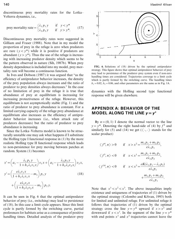
Note that if (15) holds then x3>x2>K. The partialpreference domain consists of two parts now: a part ofthe line y= y* between the points x1 and x3 and the partof the space where x>K and y> y*. Any trajectory of(1) driven by the optimal antipredator strategy thatreaches at a certain time the line y= y* between thepoints x1 and x3 will move along this line until it reachesthe point (x3, y*) where it enters the region x>K,y> y*. In this way trajectories converge to equilibriumE14 (Fig. 3A). Note that at equilibrium E14 prey popula-tion will split between both patches in the ratio

v1

v2

=m1 p1+m2 p2&eK*2 p2

eK*1 p1

. (16)

FIG. 3. Solutions of (1) driven by optimal antipredator strategywhen the refuge is limited. If carrying capacity of the refuge is low(K=4 in Fig. 3A) trajectories converge to E14. If carrying capacity ishigh (K=6.1 in Fig. 3B) then trajectories converge to a Lotka�Volterracycle which is above the line y= y* and to the left of the line x=K.Other parameters are the same as in Fig. 1A.



If (15) does not hold, the carrying capacity K is higherthan x2 and trajectories leave the line y= y* before preyabundance reaches the carrying capacity of the refuge.They enter the part of the space where y> y* where theystart to follow the corresponding Lotka�Volterra cycle.In this case, there are two possibilities. If this cycle doesnot intersect with the line x=K then trajectories behavequalitatively in the same way as in the unconstrainedcase (Fig. 1A) and no partial preferences appear. Thishappens if K is large enough. For smaller K the Lotka�Volterra cycle will intersect the line x=K that decreasesfluctuations in predator�prey dynamics (Fig. 3B). Thus,a small carrying capacity of the refuge leads to a stableequilibrium in predator prey dynamics and partialpreferences for habitats. When K is large enough, i.e.,

K�m1 p1+m2 p2

e*2 p2

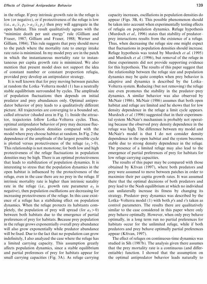
then a limit cycle appears and all prey will be in therefuge. However, the amplitude of this limit cycle issmaller than in the case of unlimited refuges since it isconstrained not only by the distance of E5 from the liney= y* but also from the line x=K. As K increases, thisdistance will also increase and at a certain moment thedistance of E5 from the line x=K will be the same as thedistance of E5 from the line y= y*. For higher values ofK the amplitude of the limit cycle measured by the dis-tance of E 5 from the line y= y* is an increasing functionof K. The dependence of the amplitude of the largestpossible fluctuations in predator�prey dynamics on thecarrying capacity K is plotted in Fig. 4.

We may also study the dependence of the amplitude oflargest fluctuations on protectiveness of the refuge

FIG. 4. The dependence of the amplitude of largest fluctuations inpopulation abundances on the carrying capacity of the refuge.Parameters a1 , a2 , m1 , m2 , e, *1 , p1 are the same as in Fig. 1A.

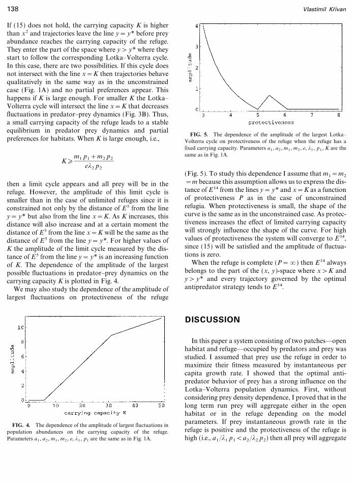
FIG. 5. The dependence of the amplitude of the largest Lotka�Volterra cycle on protectiveness of the refuge when the refuge has afixed carrying capacity. Parameters a1 , a2 , m1 , m2 , e, *1 , p1 , K are thesame as in Fig. 1A.

(Fig. 5). To study this dependence I assume that m1=m2

=m because this assumption allows us to express the dis-tance of E14 from the lines y= y* and x=K as a functionof protectiveness P as in the case of unconstrainedrefugia. When protectiveness is small, the shape of thecurve is the same as in the unconstrained case. As protec-tiveness increases the effect of limited carrying capacitywill strongly influence the shape of the curve. For highvalues of protectiveness the system will converge to E14,since (15) will be satisfied and the amplitude of fluctua-tions is zero.

When the refuge is complete (P=�) then E14 alwaysbelongs to the part of the (x, y)-space where x>K andy> y* and every trajectory governed by the optimalantipredator strategy tends to E14.

DISCUSSION

In this paper a system consisting of two patches��openhabitat and refuge��occupied by predators and prey wasstudied. I assumed that prey use the refuge in order tomaximize their fitness measured by instantaneous percapita growth rate. I showed that the optimal anti-predator behavior of prey has a strong influence on theLotka�Volterra population dynamics. First, withoutconsidering prey density dependence, I proved that in thelong term run prey will aggregate either in the openhabitat or in the refuge depending on the modelparameters. If prey instantaneous growth rate in therefuge is positive and the protectiveness of the refuge ishigh (i.e., a1 �*1 p1<a2 �*2 p2) then all prey will aggregate



in the refuge. If prey intrinsic growth rate in the refuge islow (or negative), or if protectiveness of the refuge is low(i.e., a1 �*1 p1>a2 �*2 p2) then prey will aggregate in theopen habitat. This result qualitatively agrees with the``minimize death per unit energy'' rule (Gilliam andFraser, 1987; Gilliam and Fraser, 1988; Werner andGilliam, 1984). This rule suggests that prey should moveto the patch where the mortality rate to energy intakerate ratio is minimized. In my model prey are in the patchin which the instantaneous mortality rate to instan-taneous per capita growth rate is minimized. We alsomention that present model does not support the ideaof constant number or constant proportion refugia,provided prey develop an antipredator strategy.

It is well known that for prey moving between patchesat random the Lotka�Volterra model (1) has a neutrallystable equilibrium surrounded by cycles. The amplitudeof population fluctuations then depends on initialpredator and prey abundances only. Optimal antipre-dator behavior of prey leads to a qualitatively differentpicture. All trajectories are converging to a bounded set,called attractor (shaded area in Fig. 1). Inside the attrac-tor, trajectories follow Lotka�Volterra cycles. Thus,optimal antipredator behavior of prey may decrease fluc-tuations in population densities compared with themodel where prey choose habitat at random. In Fig. 2 thedependence of the amplitude of the largest possible cycleis plotted versus protectiveness of the refuge (a2>0).This relationship is not monotone; for both low and highprotectiveness of the refuge fluctuations in populationdensities may be high. There is an optimal protectivenessthat leads to stabilization of population dynamics. It isinteresting to stress that the population dynamics in theopen habitat is influenced by the protectiveness of therefuge, even in the case there are no prey in the refuge. Ifintrinsic mortality rate is higher than intrinsic natalityrate in the refuge (i.e., growth rate parameter a2 isnegative), then population oscillations are decreasing forincreasing protectiveness of the refuge. In this case exist-ence of a refuge has a stabilizing effect on populationdynamics. When the refuge protects its habitants com-pletely, the population of prey will spread (for a2>0)between both habitats due to the emergence of partialpreferences of prey for habitats. Because prey populationin the refuge grows exponentially overall prey abundancewill also grow exponentially while predator abundancewill be fixed. Due to the fact that no population can growindefinitely, I also analyzed the case where the refuge hasa limited carrying capacity. This assumption greatlyaffects population dynamics, since a stable equilibriumand partial preferences of prey for habitats appear forsmall carrying capacities (Fig. 3A). As refuge carrying

capacity increases, oscillations in population densities doappear (Figs. 3B, 4). This possible phenomenon shouldbe taken into account when experimentally testing effectsof refugia on population dynamics. Refuge hypothesis(Murdoch et al., 1996) states that stability of predator�prey interactions results from the existence of a refuge.Thus, when decreasing the refuge size one might expectthat fluctuations in population densities should increase.Refuge hypothesis was tested by Murdoch et al. (1995)and Murdoch et al. (1996), but removal of the refuge inthese experiments did not provide supporting evidencefor this hypothesis. The results of this paper suggest thatthe relationship between the refuge size and populationdynamics may be quite complex when prey behavior isadaptive and dynamics is described by the Lotka�Volterra system. Reducing (but not removing) the refugesize even promotes the stability in the predator�preydynamics. A similar behavior was also observed byMcNair (1986). McNair (1986) assumes that both openhabitat and refuge are limited and he shows that for lowdensity dependence in the refuge a limit cycle appears.Murdoch et al. (1996) suggested that in their experimen-tal system McNair's mechanism is probably not operat-ing because the observed prey density dependence in therefuge was high. The difference between my model andMcNair's model is that I do not consider densitydependence in the open habitat and the system becomesstable due to strong density dependence in the refuge.The presence of a limited refuge may also lead to theemergence of partial preferences of prey for habitats forlow refuge carrying capacities.

The results of this paper may be compared with thoseobtained by Kr� ivan (1997), where both predators andprey were assumed to move between patches in order tomaximize their per capita growth rates. It was assumedthere that the optimal decisions of both predators andprey lead to the Nash equilibrium at which no individualcan unilaterally increase its fitness by changing itsstrategy. Predator�prey dynamics was described by theLotka�Volterra model (1) with both p's and v's taken ascontrol parameters. The results there are qualitativelysimilar to the case considered in this paper where onlyprey behave optimally. However, when only prey behaveoptimally, in a long term run no partial preferences forhabitats occur for the unlimited refuge, while if bothpredators and prey behave optimally partial preferencesappear (Kr� ivan, 1997).

The effect of refuges on continuous-time dynamics wasstudied in Sih (1987b). The analysis given there assumesthat the prey mortality rate is a continuous (and differ-entiable) function. I showed that the assumption onthe optimal antipredator behavior leads naturally to



discontinuous prey mortality rates for the Lotka�Volterra dynamics, i.e.,

prey mortality rate={*1 p1 y*2 p2 y

if y< y*if y> y*.

(17)

Discontinuous prey mortality rates were suggested inGilliam and Fraser (1988). Note that in my model theproportion of prey in the refuge is zero when predatorsare rare ( y< y*) while it is positive if predators areabundant ( y> y*). Thus the use of the refuge is increas-ing with increasing predator density which seems to bethe pattern observed in nature (Sih, 1987b). When preydensity dependence is included into my model, prey mor-tality rate will become a continuous function.

In Ives and Dobson (1987) it was argued that ``as theefficiency of antipredator behavior increases, the densityof the prey population always increases and the ratio ofpredator to prey densities always decreases.'' In the caseof no limitation of prey in the refuge it is true thatabundance of prey at equilibrium is increasing forincreasing protectiveness of the refuge. However, thisequilibrium is not asymptotically stable (Fig. 1) and theratio of predator to prey abundance is constant. For alimited carrying capacity of the refuge prey abundance atequilibrium also increases as the efficiency of antipre-dator behavior increases (i.e., when attack rate ofpredators decreases) but the ratio of predator to preyabundance is increasing.

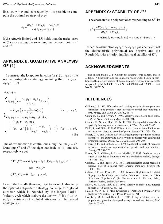
Since the Lotka�Volterra model is known to be struc-turally unstable one may ask what happens if I substitutethe Holling type I functional response in (1) by the morerealistic Holling type II functional response which leadsto non-persistence for prey moving between patches atrandom. System (1) becomes

x$=\a1&*1 p1 y

1+h1*1 v1x+ v1x+\a2&*2 p2 y

1+h2*2v2 x+ v2x,

y$=\ e*1v1x1+h1*1v1 x

&m1+ p1 y (18)

+\ e*2v2x1+h2 *2v2 x

&m2+ p2 y.

It can be seen in Fig. 6 that the optimal antipredatorbehavior of prey (i.e., switching) may lead to persistenceof (18). In this case a limit cycle appears. Since this limitcycle is partly formed by the switching curve, partialpreferences for habitats arise as a consequence of positivehandling times. Detailed analysis of the predator�prey

FIG. 6. Solutions of (18) driven by the optimal antipredatorstrategy. This figure shows that optimal antipredator behavior of preymay lead to persistence of the predator�prey system even if non-zerohandling times are considered. Trajectories converge to a limit cyclewhich is partly formed by the switching curve. The handling timesh1=0.02, h2=0.06, and other parameters are the same as in Fig. 1A.

dynamics with the Holling second type functionalresponse will be given elsewhere.

APPENDIX A: BEHAVIOR OF THEMODEL ALONG THE LINE y=y*

By n=(0, 1) I denote the normal vector to the liney= y*. Denoting the right hand-side of (4) by f 4 andsimilarly for (5) and (14) we get (( } , } ) stands for thescalar product)

( f 4, n) >0 if x>x2=m1 p1+m2 p2

e*1 p1

,

( f 5, n) <0 if x<x1=m1 p1+m2 p2

e*2 p2

,

( f 14, n) <0 if x<x3=eK(*1 p1&*2 p2)

e*1 p1

+m1 p1+m2 p2

e*1 p1

.

Note that x1<x2<x3. The above inequalities implyexistence and uniqueness of trajectories of (1) driven bythe optimal strategy (Colombo and Kr� ivan, 1993) bothfor limited and unlimited refuge. For unlimited refuge itfollows that trajectories of (1) driven by the optimalstrategy cross the line y= y* upward if x>x2 anddownward if x<x1. In the segment of the line y= y*with end points x1 and x2 trajectories cannot leave the



line, i.e., y$=0 and, consequently, it is possible to com-pute the optimal strategy of prey

v1=m1 p1+m2 p2&e*2 p2x

ex(*1 p1&*2 p2).

If the refuge is limited and (15) holds than the trajectoriesof (1) move along the switching line between points x1

and x3.

APPENDIX B: QUALITATIVE ANALYSISOF (1)

I construct the Lyapunov function for (1) driven by theoptimal antipredator strategy assuming that a1*2 p2<a2 *1 p1 . Let

V(x, y)=

e*2 p2 \x&m1 p1+m2 p2

e*2 p2

ln(x)++*2 p2 \y&

a2

*2 p2

ln( y)+ for y> y*,

e*2 p2 x&(m1 p1+m2 p2) ln(x)

+*1 p1 y&a1 ln( y)

+(a1&a2) \ln \ a1&a2

*1 p1&*2 p2 +&1+ for y� y*.

(19)

The above function is continuous along the line y= y*.Denoting f 4 and f 5 the right handside of (4) and (5),respectively we get

(V$, f 4) =ex(*2 p2&*1 p1)(a1&*1 p1 y)<0

for y� y*

(V$, f 5) =0 for y> y*.

Due to the LaSalle theorem, trajectories of (1) driven bythe optimal antipredator strategy converge to a globalattractor which is bounded by the largest Lotka�Volterra cycle which is above the line y= y*. If a1*2 p2>a2 *1 p1 existence of a global attractor can be provedanalogously.

APPENDIX C: STABILITY OF E14

The characteristic polynomial corresponding to E 14 is:

_2+eK(a2 *1 p1&a1 *2 p2)

m1 p1+m2 p2

_

+eK(a2*1 p1&a1*2 p2)+a1(m1 p1+m2 p2).

Under the assumption a2*1 p1>a1 *2 p2 all coefficients ofthe characteristic polynomial are positive and theRouth�Hurwitz criterion implies local stability of E 14.

ACKNOWLEDGMENTS

The author thanks J. F. Gilliam for sending some papers, and toJ. Titus, O. J. Schmitz, and six unknown reviewers for helpful sugges-tions on the previous version of the manuscript. This work was partiallysupported by MS8 MT C8 R (Grant No. VS 96086) and GA C8 R (GrantNo. 201�98�0227).

REFERENCES

Collings, J. B. 1995. Bifurcation and stability analysis of a temperature-dependent mite predator�prey interaction model incorporating aprey refuge, Bull. Math. Biology 57, 63�76.

Colombo, R., and Kr� ivan, V. 1993. Selective strategies in food webs,IMA J. Math. Appl. Med. Biol. 10, 281�291.

Comins, H. N., and Blatt, D. W. E. 1974. Prey�predator models inspatially heterogeneous environments, J. Theor. Biol. 48, 75�83.

Diehl, S., and Eklo� v, P. 1995. Effects of piscivore-mediated habitat useon resources, diet, and growth of perch, Ecology 76, 1712�1726.

Fraser, D. F., and Gilliam, J. F. 1987. Feeding under predation hazard:response of the guppy and hart's rivulus from sites with contrastingpredation hazard, Behav. Ecol. Sociobiol. 21, 203�209.

Fraser, D. F., and Gilliam, J. F. 1992. Nonlethal impacts of predatorinvasion: Facultative suppression of growth and reproduction,Ecology 73, 959�970.

Fraser, D. F., Gilliam, J. F., and Yip-Hoi, T. 1995. Predation as anagent of population fragmentation in a tropical watershed, Ecology76, 1461�1472.

Gilliam, J. F., and Fraser, D. F. 1987. Habitat selection under predationhazard: Test of a model with foraging minnows, Ecology 68,1856�1862.

Gilliam, J. F., and Fraser, D. F. 1988. Resource Depletion and HabitatSegregation by Competitors under Predation Hazard, in ``Size-Structured Populations'' (B. Ebenman and L. Perrson, Eds.),Springer-Verlag, Berlin�New York.

Hassel, M. P., and May, R. M. 1973. Stability in insect host-parasitemodels, J. An. Ecol. 42, 693�725.

Hassell, M. P. 1978. ``The Dynamics of Arthropod Predator�PreySystems,'' Princeton Univ. Press, Princeton, NJ.

Hochberg, M. E., and Holt, R. D. 1995. Refuge evolution and thepopulation dynamics of coupled host-parasitoid associations, Evol.Ecol. 9, 633�661.



Holt, R. D. 1983. Optimal foraging and the form of the predatorisocline, Am. Naturalist 122, 521�541.

Holt, R. D. 1985. Population dynamics in two-patch environments:Some anomalous consequences of an optimal habitat distribution,Theor. Popul. Biol. 28, 181�208.

Holt, R. D. 1987. Prey communities in patchy environments, Oikos 50,276�290.

Ives, A. R., and Dobson, A. P. 1987. Antipredator behavior and thepopulation dynamics of simple predator�prey systems, Am.Naturalist 130, 431�447.

Kr� ivan, V. 1997. Dynamic ideal free distribution: Effects of optimalpatch choice on predator�prey dynamics, Am. Naturalist 149,164�178.

Lima, S. L., and Dill, L. M. 1990. Behavioral decisions made under therisk of predation: A review and prospectus, Can. J. Zool. 68,619�640.

Maynard Smith, J. 1974. ``Models in Ecology,'' Cambridge Univ. Press,Cambridge, UK.

McNair, J. N. 1986. The effects of refuges on predator�prey interac-tions: A reconsideration, Theor. Popul. Biol. 29, 38�63.

Mittelbach, G. G., and Chesson, P. L. 1987. Predation risk: Indirecteffects on fish populations, in ``Predation'' (W. C. Kerfoot and A. Sih,Eds.), Univ. press of New England, Hanover.

Murdoch, W. W., and Stewart-Oaten, A. 1975. Predation and popula-tion stability, Adv. Ecol. Res. 9, 1�131.

Murdoch, W. W., Luck, R. F., Swarbrick, S. L., Walde, S., Yu, D. S.,and Reeve, J. D. 1995. Regulation of an insect population underbiological control, Ecology 76, 206�217.

Murdoch, W. W., Swarbrick, S. L., Luck, R., Walde, S., and Yu, D. S.1996. Refuge dynamics and metapopulation dynamics: Anexperimental test, Am. Naturalist 147, 424�444.

Rosenzweig, M. L., and MacArthur, R. H. 1963. Graphical representa-tion and stability conditions of predator�prey interactions, Am.Naturalist 97, 209�223.

Ruxton, G. D. 1995. Short term refuge use and stability of predator�prey models, Theor. Popul. Biol. 47, 1�17.

Sih, A. 1980. Optimal behavior: Can foragers balance two conflictingdemands?, Science 210, 1041�1043.

Sih, A. 1986. Antipredator responses and the preception of danger bymosquito larvae, Ecology 67, 434�441.

Sih, A. 1987a. Predators and prey lifestyles: An evolutionary overview,in ``Predation'' (W. C. Kerfoot and A. Sih, Eds.), Univ. Press of NewEngland, Hanover.

Sih, A. 1987b. Prey refuges and predator�prey stability, Theor. Popul.Biol. 31, 1�12.

Werner, E. E., and Gilliam, J. F. 1984. The ontogenetic niche and speciesinteractions in size-structured populations, Ann. Rev. Ecol. Syst..

Werner, E. E., Gilliam, J. F., Hall, D. J., and Mittelbach, G. G. 1983.An experimental test of the effects of predation risk on habitat use infish, Ecology 64, 1540�1548.

� � � � � � � � � � � � � � � � � � � �


Documents

Effects of Optimal Antipredator Behavior of Prey on Predatorâ€“Prey