Embed Size (px)
DESCRIPTION
Efficient Access to Remote Data in High Energy Physics. René Brun, Leandro Franco, Fons Rademakers. CERN Geneva, Switzerland. Roadmap. Current Status Problem Taking Advantage of ROOT Solution Limitations Future Work Conclusions. Motivation. - PowerPoint PPT Presentation
Citation preview
Leandro Franco
Efficient Access to Remote Data inEfficient Access to Remote Data inHigh Energy PhysicsHigh Energy Physics
René Brun, Leandro Franco, Fons Rademakers
CERNGeneva, Switzerland
2Leandro Franco
RoadmapRoadmap
• Current Status
• Problem
• Taking Advantage of ROOT
• Solution
• Limitations
• Future Work
• Conclusions
3Leandro Franco
MotivationMotivation
• ROOT was designed to process files locally or in local area networks.
• Reading trees across wide area networks involved a big number of transactions. Therefore, processing in high latency networks was inefficient.
• If we want to process the whole file (or a big part of it), it’s better to transfer it locally first.
• If we want to process only a small part of the file, transferring it would be wasteful and we would prefer to access it remotely.

4Leandro Franco
Traditional SolutionTraditional Solution• The way this problem has been treated is always the
same (old versions of ROOT, RFIO, dCache, etc):• Transfer data by blocks of a given size. For instance, if a block of
len 64KB in the position 1000KB of the file is requested, it doesn’t just transfer the 64KB but a big chunk of 1MB starting at 1000KB.
1. Read(buf, 64kB, 1000KB)
2. Read(buf, 64kB, 1064KB)• It is found in the
cache• Read it locally
len offset
Offset = 0 Offset = 1000KB
len = 64KB len = 1MB
• This works well when two conditions are met:• We read sequentially• We read the whole file.
Server SideServer SideClient SideClient SideRead(buf, 64kB, 1000KB)
Return the read-ahead buffer
5Leandro Franco
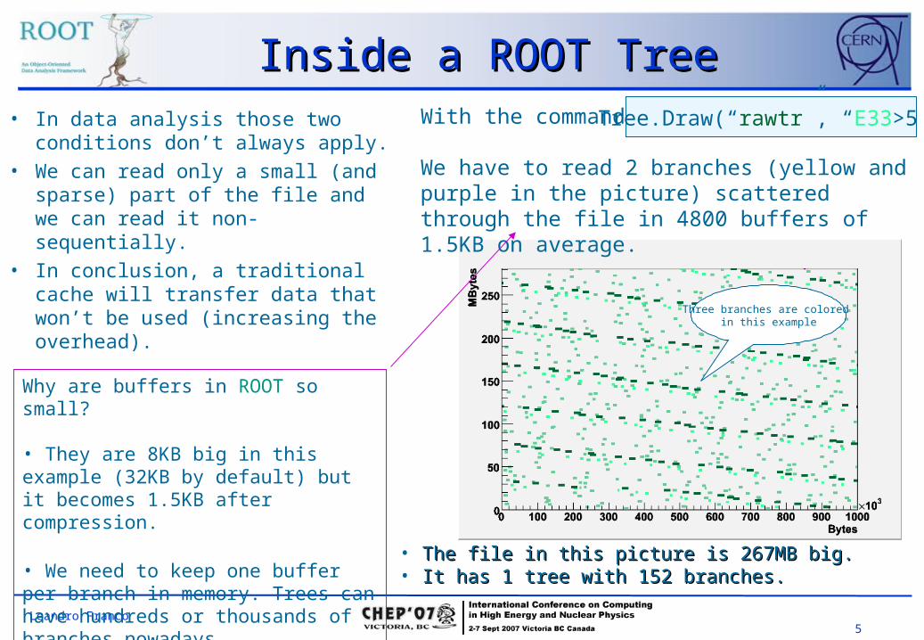
Inside a ROOT TreeInside a ROOT Tree• In data analysis those two
conditions don’t always apply.• We can read only a small (and
sparse) part of the file and we can read it non-sequentially.
• In conclusion, a traditional cache will transfer data that won’t be used (increasing the overhead).
Three branches are colored in this example
With the command:
We have to read 2 branches (yellow and purple in the picture) scattered through the file in 4800 buffers of 1.5KB on average.
• The file in this picture is 267MB big.The file in this picture is 267MB big.• It has 1 tree with 152 branches.It has 1 tree with 152 branches.
Tree.Draw(“rawtr”, “E33>5”)
Why are buffers in ROOT so small?
• They are 8KB big in this example (32KB by default) but it becomes 1.5KB after compression.
• We need to keep one buffer per branch in memory. Trees can have hundreds or thousands of branches nowadays.
6Leandro Franco
Facing Various Latency Facing Various Latency Problems Problems
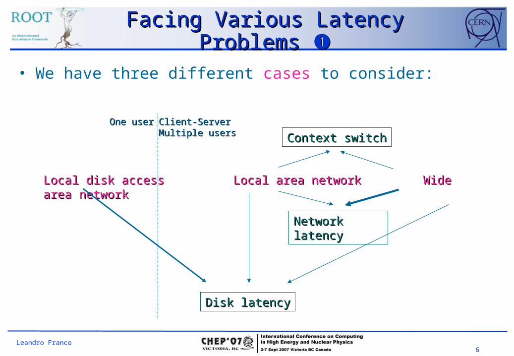
• We have three different cases to consider:
Local disk accessLocal disk access Local area networkLocal area network Wide area networkWide area network
Network latencyNetwork latency
Disk latencyDisk latency
Context switchContext switch
One userOne user Client-ServerClient-ServerMultiple usersMultiple users
7Leandro Franco
Facing Various Latency Facing Various Latency Problems Problems
How can we overcome the problems in these three cases ?:
• Disk latency: Is an issue in all the cases but it’s the only one when doing local readings.• Can be reduced by reading sequentially and in big blocks (less
transactions).
• Context switching: Is a problem for loaded servers. Since they have to serve multiple users, they are forced to switch between processes (switching is usually fast but doing it often can produce a noticeable overhead).• Can be very harmful if it’s combined with disk latency.• It helps to reduce the number of transaction and/or the time between them.
• Network latency: It increases proportionally to the distance between the client and the server. It’s a big issue when reading scattered data through long distances.• Reducing the number of transactions will improve the performance.
8Leandro Franco
Data Access Parameters Data Access Parameters
file1
file2
file3
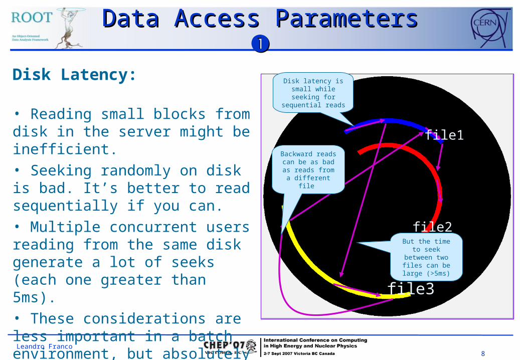
Disk latency is small while seeking for
sequential reads
But the time to seek between
two files can be large (>5ms)
Backward reads can be as bad as
reads from a different file
Disk Latency:
• Reading small blocks from disk in the server might be inefficient.• Seeking randomly on disk is bad. It’s better to read sequentially if you can.• Multiple concurrent users reading from the same disk generate a lot of seeks (each one greater than 5ms).• These considerations are less important in a batch environment, but absolutely vital for interactive applications.
9Leandro Franco
Data Access Parameters Data Access Parameters
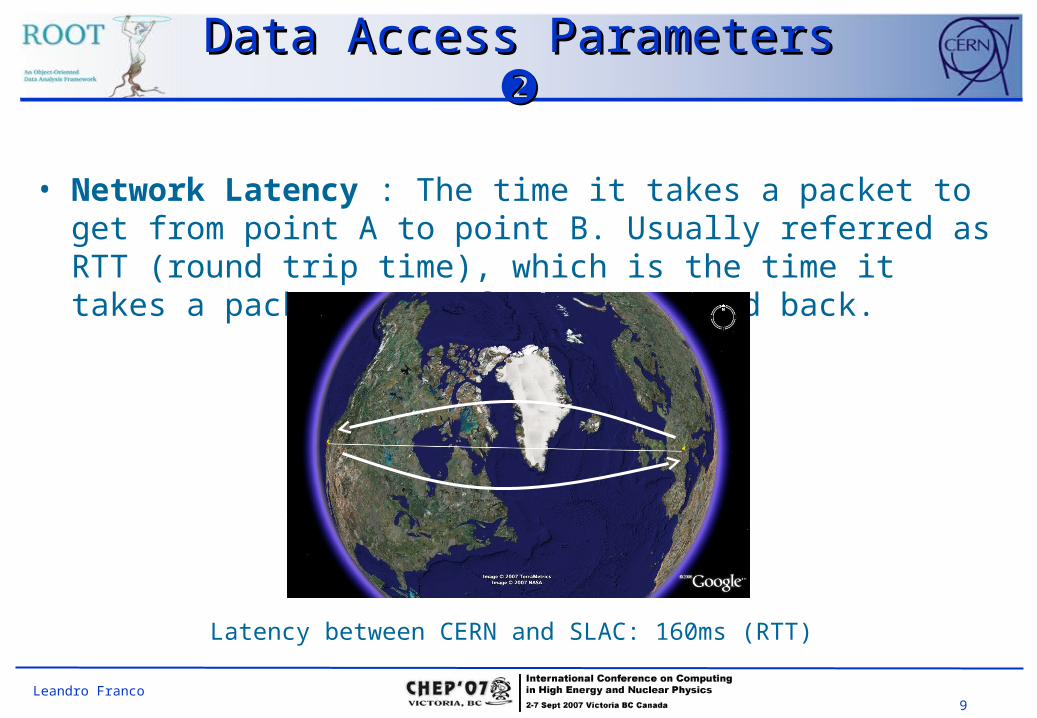
• Network Latency : The time it takes a packet to get from point A to point B. Usually referred as RTT (round trip time), which is the time it takes a packet to go from A to B and back.
Latency between CERN and SLAC: 160ms (RTT)
10Leandro Franco
Data Access Parameters Data Access Parameters
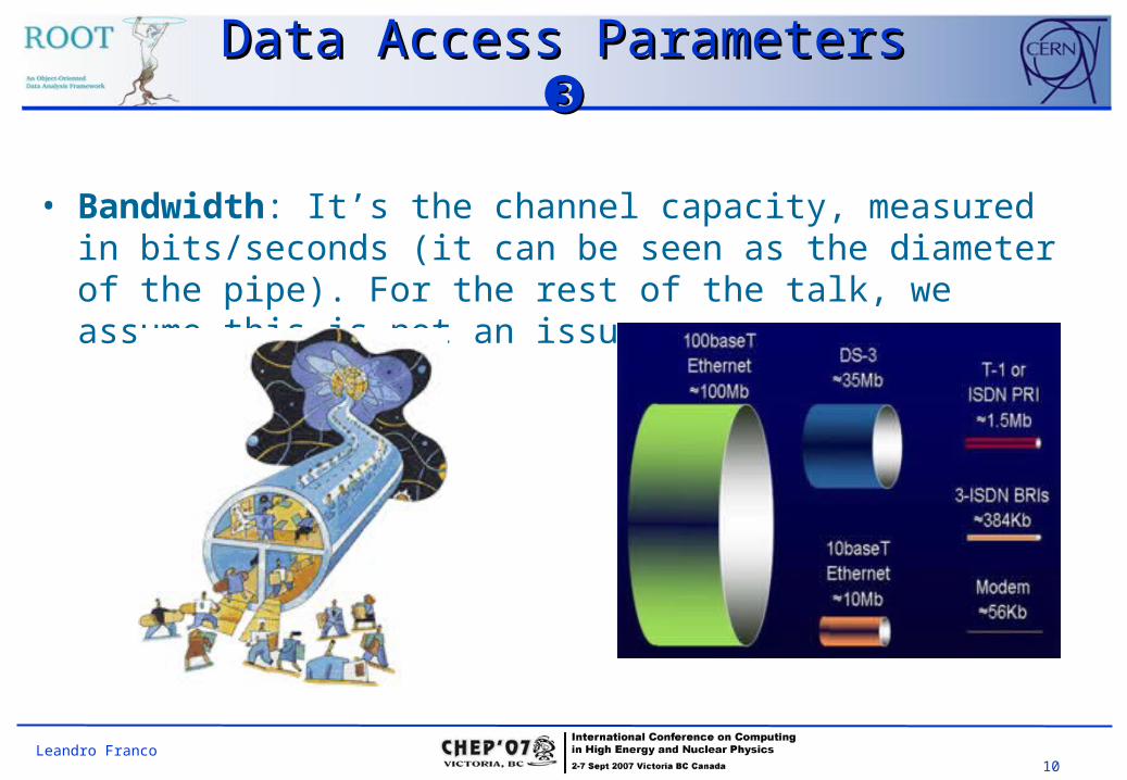
• Bandwidth: It’s the channel capacity, measured in bits/seconds (it can be seen as the diameter of the pipe). For the rest of the talk, we assume this is not an issue.

11Leandro Franco
ProblemProblem• While processing a large (remote) file the data
has, so far, been transferred in small chunks.• It doesn’t matter how many chunks you can carry if you will only
read them one by one.
• In ROOT, each of those small chunks is usually spread out in a big file.
• The time spent exchanging messages to get the data could be a considerable part of the total time.
• This becomes a problem when we have high latency connections (independently of bandwidth).
12Leandro Franco
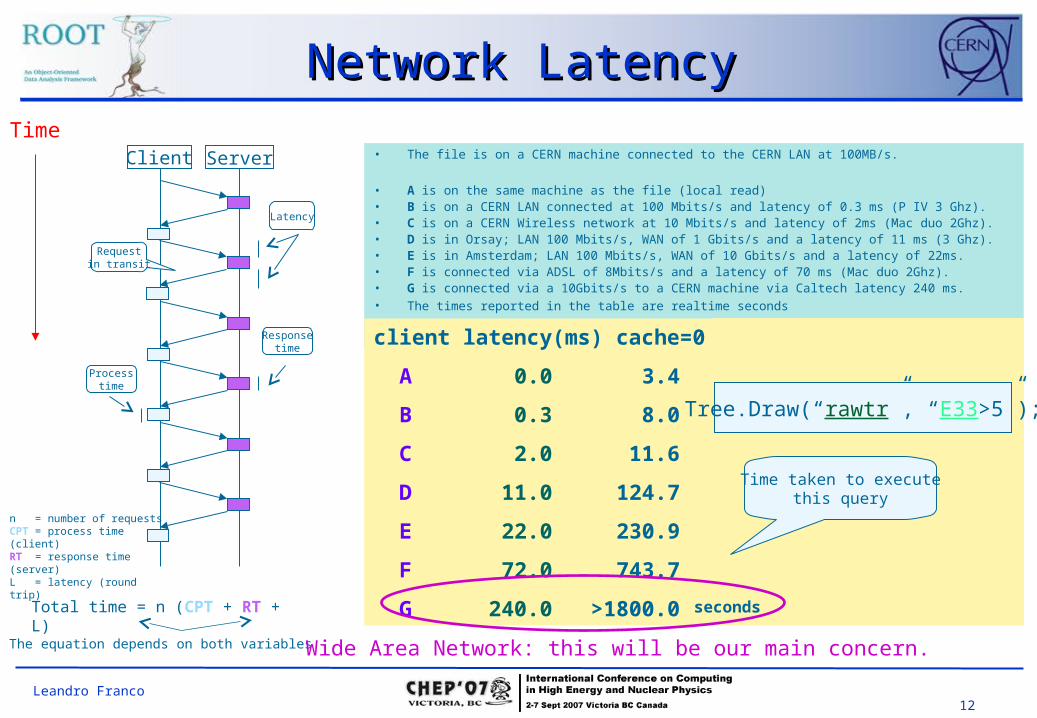
Network LatencyNetwork Latency
Client Server
Time
Requestin transit
Latency
Responsetime
Processtime
Total time = n (CPT + RT + L)
n = number of requests CPT = process time (client)RT = response time (server)L = latency (round trip)
The equation depends on both variables
• The file is on a CERN machine connected to the CERN LAN at 100MB/s.
• A is on the same machine as the file (local read) • B is on a CERN LAN connected at 100 Mbits/s and latency of 0.3 ms (P IV 3 Ghz). • C is on a CERN Wireless network at 10 Mbits/s and latency of 2ms (Mac duo 2Ghz). • D is in Orsay; LAN 100 Mbits/s, WAN of 1 Gbits/s and a latency of 11 ms (3 Ghz). • E is in Amsterdam; LAN 100 Mbits/s, WAN of 10 Gbits/s and a latency of 22ms. • F is connected via ADSL of 8Mbits/s and a latency of 70 ms (Mac duo 2Ghz). • G is connected via a 10Gbits/s to a CERN machine via Caltech latency 240 ms.• The times reported in the table are realtime seconds
client latency(ms) cache=0 cache=64KB cache=10MB
A 0.0 3.4 3.4 3.4
B 0.3 8.0 6.0 4.0
C 2.0 11.6 5.6 4.9
D 11.0 124.7 12.3 9.0
E 22.0 230.9 11.7 8.4
F 72.0 743.7 48.3 28.0
G 240.0 >1800.0 125.4 9.9
Wide Area Network: this will be our main concern.
Tree.Draw(“rawtr”, “E33>5”);
Time taken to executethis query
seconds
13Leandro Franco
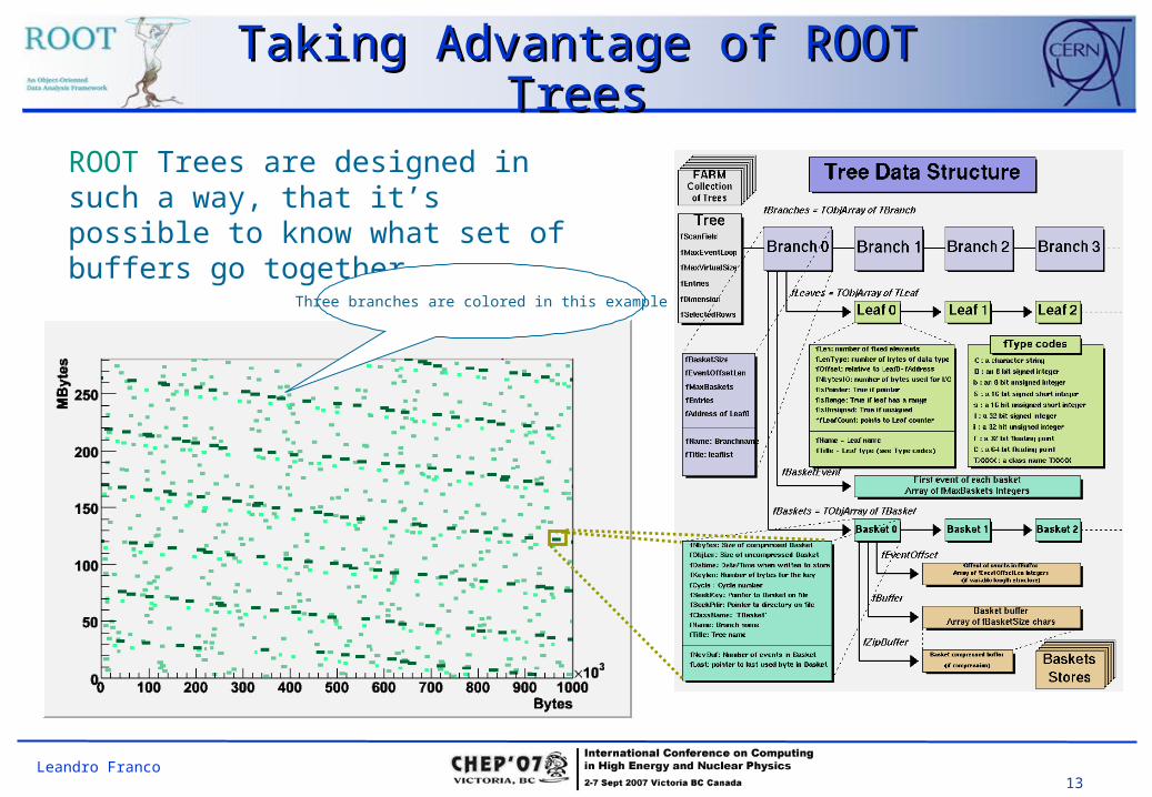
Taking Advantage of ROOT Taking Advantage of ROOT TreesTrees
ROOT Trees are designed in such a way, that it’s possible to know what set of buffers go together.
Three branches are colored in this example
14Leandro Franco
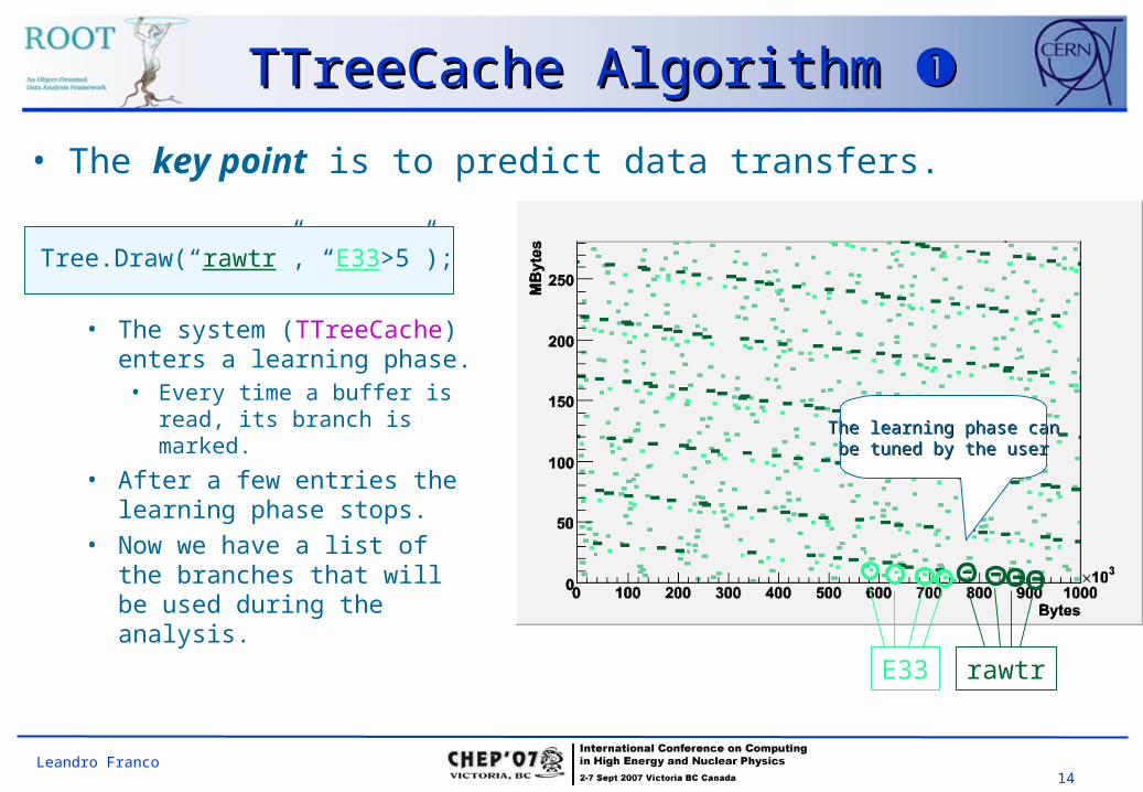
TTreeCache Algorithm TTreeCache Algorithm
• The key point is to predict data transfers.
Tree.Draw(“rawtr”, “E33>5”);
• The system (TTreeCache) enters a learning phase.• Every time a buffer is
read, its branch is marked.
• After a few entries the learning phase stops.
• Now we have a list of the branches that will be used during the analysis.
rawtrE33
The learning phase canThe learning phase canbe tuned by the userbe tuned by the user
15Leandro Franco
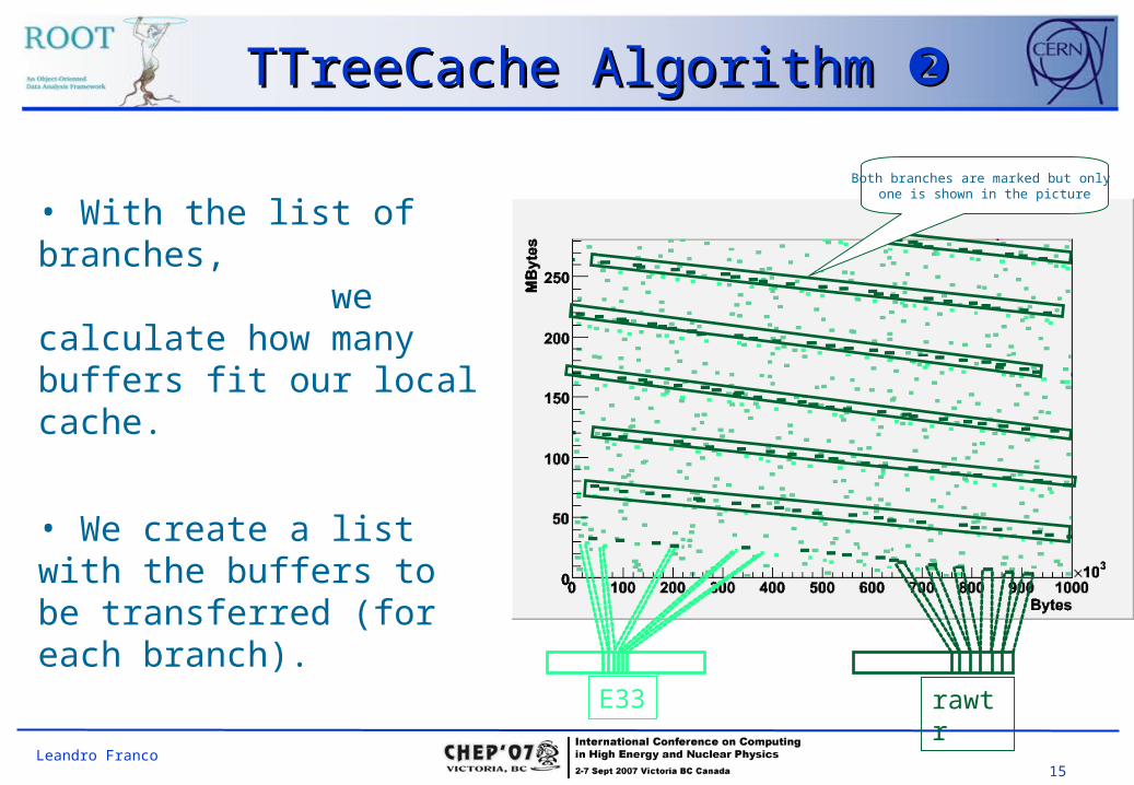
TTreeCache Algorithm TTreeCache Algorithm
rawtrE33
• With the list of branches, we calculate how many buffers fit our local cache.
• We create a list with the buffers to be transferred (for each branch).
*Both branches add up to 4800 buffers of 1.5KB on average.
Both branches are marked but only one is shown in the picture
16Leandro Franco
TTreeCache Algorithm TTreeCache Algorithm
rawtrE33
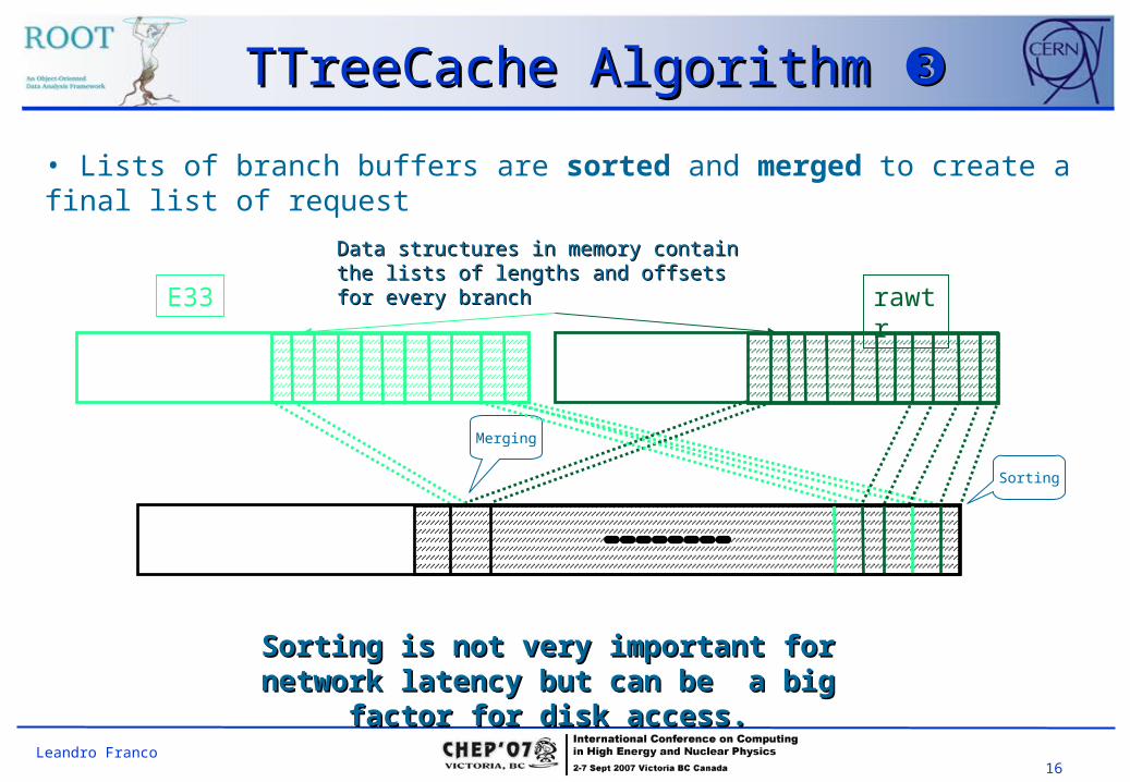
• Lists of branch buffers are sorted and merged to create a final list of request
Sorting
Merging
Sorting is not very important for network Sorting is not very important for network latency but can be a big factor for disk access.latency but can be a big factor for disk access.
Data structures in memory contain the lists of Data structures in memory contain the lists of lengths and offsets for every branchlengths and offsets for every branch
17Leandro Franco
Servers Require Protocol Servers Require Protocol ExtensionsExtensions
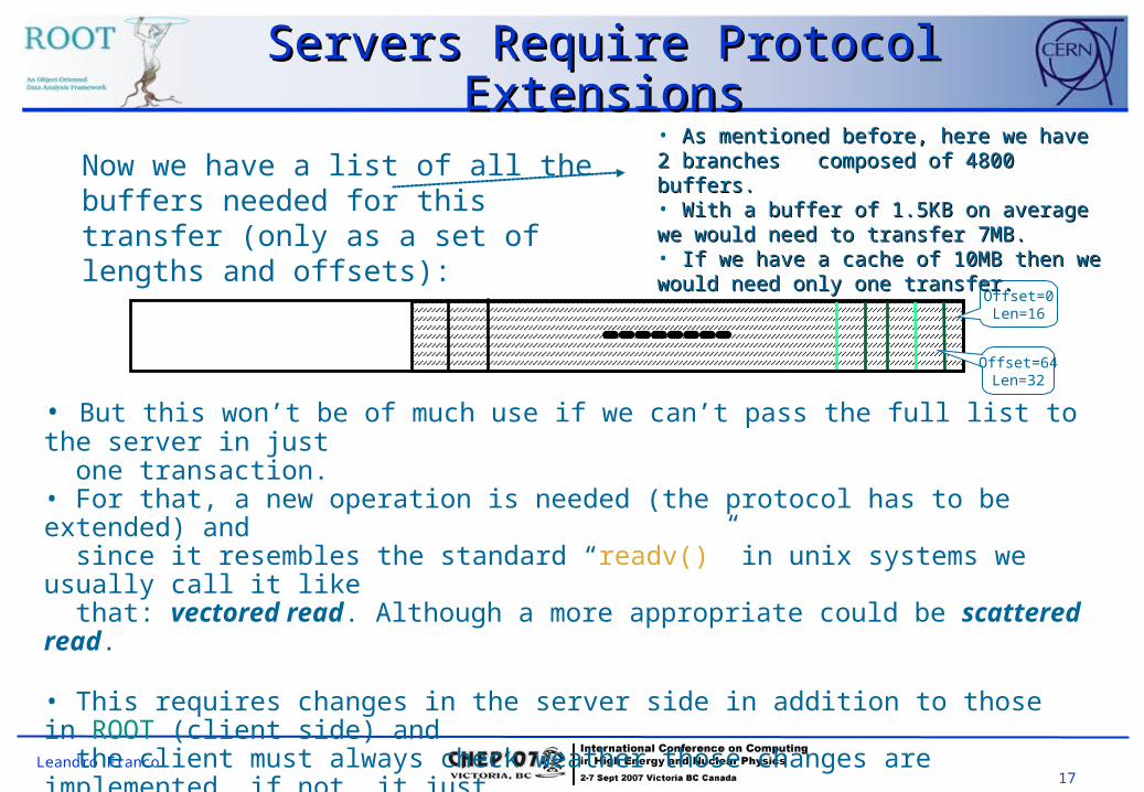
Now we have a list of all the buffers needed for this transfer (only as a set of lengths and offsets):
Offset=0Len=16
Offset=64Len=32
• But this won’t be of much use if we can’t pass the full list to the server in just one transaction.• For that, a new operation is needed (the protocol has to be extended) and since it resembles the standard “readv()” in unix systems we usually call it like that: vectored read. Although a more appropriate could be scattered read.
• This requires changes in the server side in addition to those in ROOT (client side) and the client must always check weather those changes are implemented, if not, it just uses the old method.• We have introduced the changes in rootd, xrootd and http. The dCache team introduced it in a beta release for their server and the dCache ROOT client.
• As mentioned before, here we have 2 branches As mentioned before, here we have 2 branches composed of 4800 buffers. composed of 4800 buffers.• With a buffer of 1.5KB on average we would With a buffer of 1.5KB on average we would need to transfer 7MB.need to transfer 7MB.• If we have a cache of 10MB then we would If we have a cache of 10MB then we would need only one transfer.need only one transfer.
18Leandro Franco
SolutionSolution
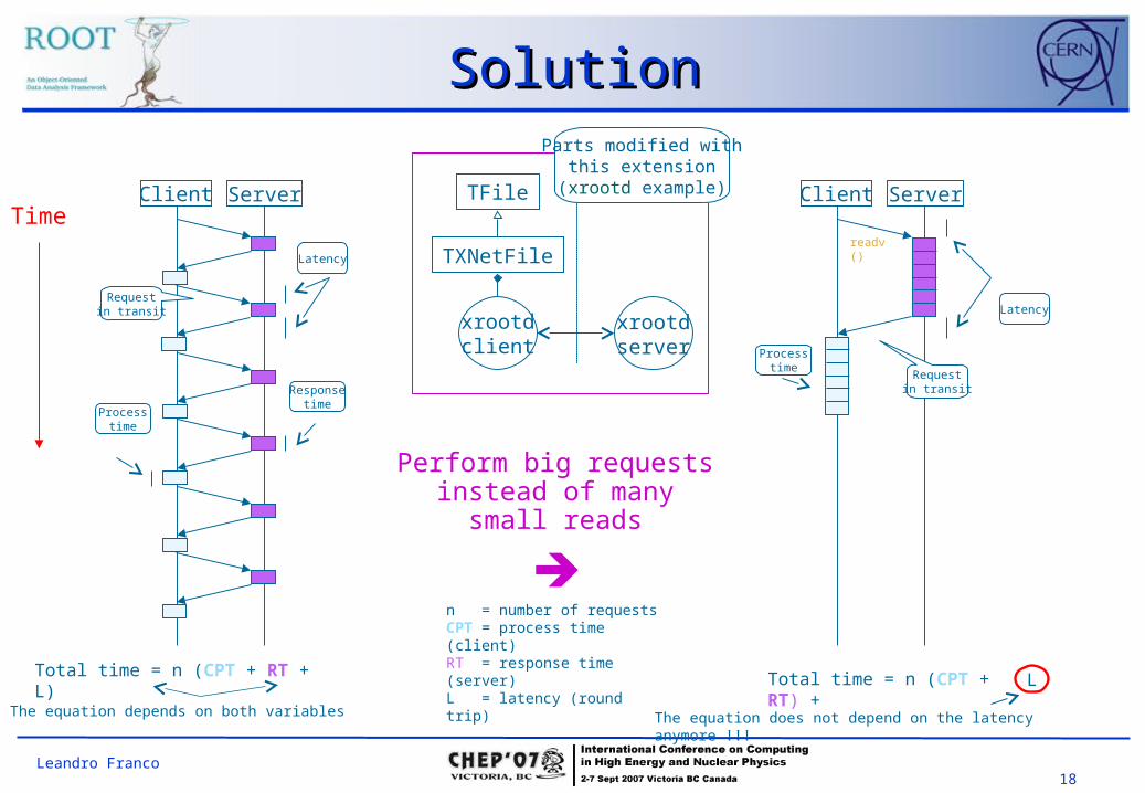
LTotal time = n (CPT + RT) +
The equation does not depend on the latency anymore !!!
n = number of requests CPT = process time (client)RT = response time (server)L = latency (round trip)
Client Server
Requestin transit
Latency
Processtime
readv()
Client ServerTime
Requestin transit
Latency
Responsetime
Processtime
Total time = n (CPT + RT + L)
The equation depends on both variables
Perform big requests instead of many small
reads
TFile
TXNetFile
xrootdclient
xrootdserver
Parts modified withthis extension
(xrootd example)
19Leandro Franco
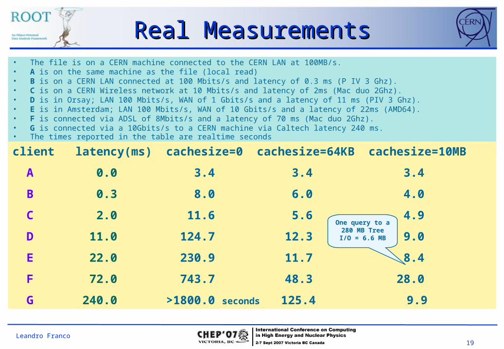
Real MeasurementsReal Measurements• The file is on a CERN machine connected to the CERN LAN at 100MB/s. • A is on the same machine as the file (local read) • B is on a CERN LAN connected at 100 Mbits/s and latency of 0.3 ms (P IV 3 Ghz). • C is on a CERN Wireless network at 10 Mbits/s and latency of 2ms (Mac duo 2Ghz). • D is in Orsay; LAN 100 Mbits/s, WAN of 1 Gbits/s and a latency of 11 ms (PIV 3 Ghz). • E is in Amsterdam; LAN 100 Mbits/s, WAN of 10 Gbits/s and a latency of 22ms (AMD64). • F is connected via ADSL of 8Mbits/s and a latency of 70 ms (Mac duo 2Ghz). • G is connected via a 10Gbits/s to a CERN machine via Caltech latency 240 ms.• The times reported in the table are realtime seconds
client latency(ms) cachesize=0 cachesize=64KB cachesize=10MB
A 0.0 3.4 3.4 3.4
B 0.3 8.0 6.0 4.0
C 2.0 11.6 5.6 4.9
D 11.0 124.7 12.3 9.0
E 22.0 230.9 11.7 8.4
F 72.0 743.7 48.3 28.0
G 240.0 >1800.0 seconds 125.4 9.9
One query to a 280 MB TreeI/O = 6.6 MB
20Leandro Franco
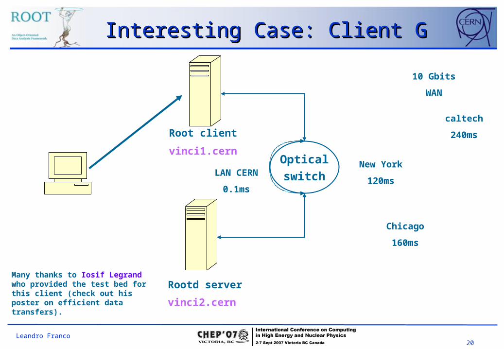
Opticalswitch
Root client
vinci1.cern
Rootd server
vinci2.cern
Chicago
160ms
New York
120ms
LAN CERN
0.1ms
10 Gbits
WAN
Many thanks to Iosif Legrand who provided the test bed for this client (check out his poster on efficient data transfers).
caltech
240ms
Interesting Case: Client GInteresting Case: Client G
21Leandro Franco
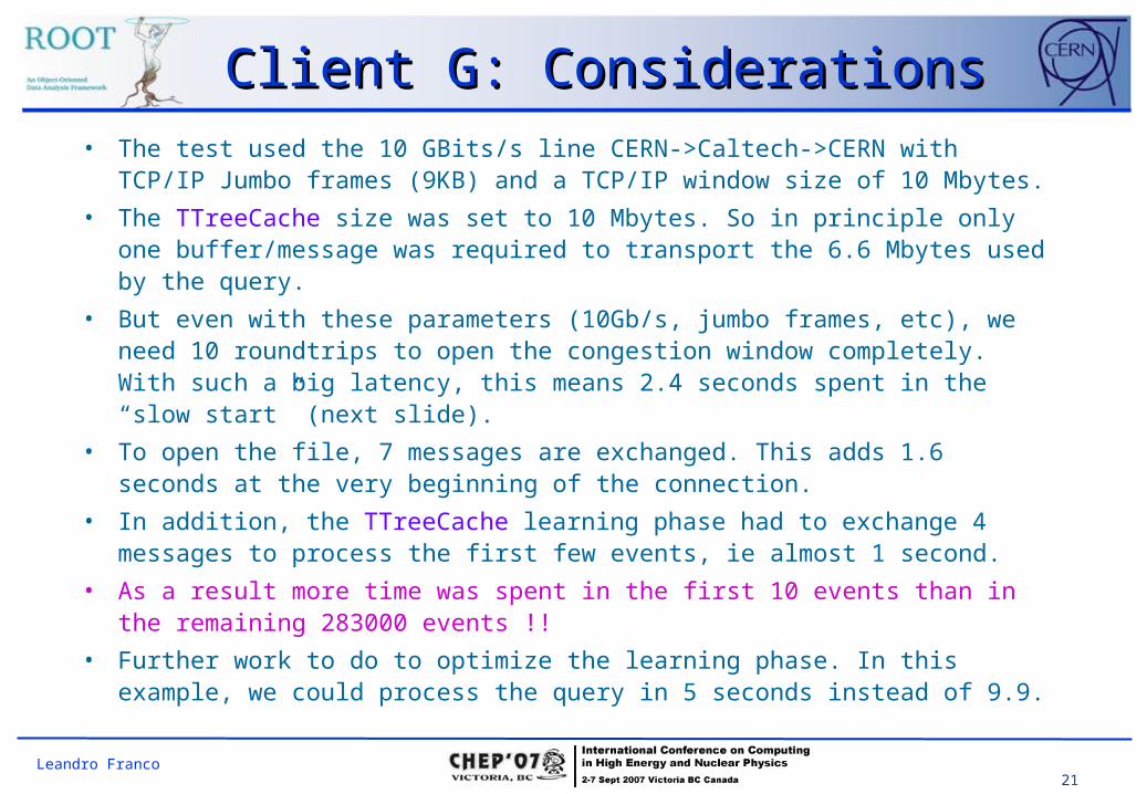
Client G: ConsiderationsClient G: Considerations• The test used the 10 GBits/s line CERN->Caltech->CERN with TCP/IP
Jumbo frames (9KB) and a TCP/IP window size of 10 Mbytes.
• The TTreeCache size was set to 10 Mbytes. So in principle only one buffer/message was required to transport the 6.6 Mbytes used by the query.
• But even with these parameters (10Gb/s, jumbo frames, etc), we need 10 roundtrips to open the congestion window completely. With such a big latency, this means 2.4 seconds spent in the “slow start” (next slide).
• To open the file, 7 messages are exchanged. This adds 1.6 seconds at the very beginning of the connection.
• In addition, the TTreeCache learning phase had to exchange 4 messages to process the first few events, ie almost 1 second.
• As a result more time was spent in the first 10 events than in the remaining 283000 events !!
• Further work to do to optimize the learning phase. In this example, we could process the query in 5 seconds instead of 9.9.
22Leandro Franco
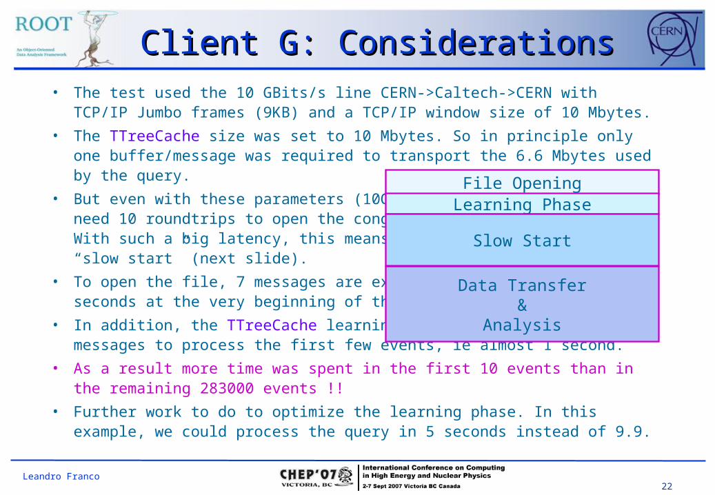
• The test used the 10 GBits/s line CERN->Caltech->CERN with TCP/IP Jumbo frames (9KB) and a TCP/IP window size of 10 Mbytes.
• The TTreeCache size was set to 10 Mbytes. So in principle only one buffer/message was required to transport the 6.6 Mbytes used by the query.
• But even with these parameters (10Gb/s, jumbo frames, etc), we need 10 roundtrips to open the congestion window completely. With such a big latency, this means 2.4 seconds spent in the “slow start” (next slide).
• To open the file, 7 messages are exchanged. This adds 1.6 seconds at the very beginning of the connection.
• In addition, the TTreeCache learning phase had to exchange 4 messages to process the first few events, ie almost 1 second.
• As a result more time was spent in the first 10 events than in the remaining 283000 events !!
• Further work to do to optimize the learning phase. In this example, we could process the query in 5 seconds instead of 9.9.
Client G: ConsiderationsClient G: Considerations
File OpeningLearning Phase
Slow Start
Data Transfer&
Analysis
23Leandro Franco
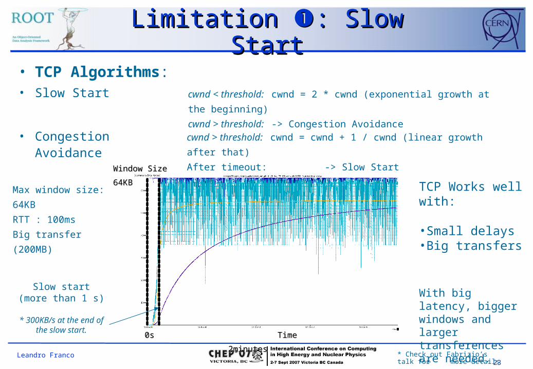
Limitation Limitation : Slow Start: Slow Start• TCP Algorithms:• Slow Start
• Congestion Avoidance
cwnd < threshold: cwnd = 2 * cwnd (exponential growth at the
beginning)
cwnd > threshold: -> Congestion Avoidancecwnd > threshold: cwnd = cwnd + 1 / cwnd (linear growth
after that)
After timeout: -> Slow Start (threshold=cwnd/2 ,
cwnd=1)
* Check out Fabrizio’s talk for more details
Max window size:
64KB
RTT : 100ms
Big transfer
(200MB)
TCP Works well with:
•Small delays•Big transfers
With big latency, bigger windows and larger transferences are needed.
Slow start(more than 1 s)
* 300KB/s at the end of the slow start.
Window SizeWindow Size
64KB64KB
0s0s Time Time
2minutes2minutes
24Leandro Franco
Limitation Limitation : Transfer : Transfer sizesize
• To transfer all the data in a single request is not realistic. The best we can do is to transfer blocks big enough to improve the performance.
• Let's say our small blocks are usually 2.5KB big, if we have a buffer of 256KB we will be able to perform 100 requests in a single transfer.
• But even then we will be limited by the maximum size of the congestion window in TCP (in our examples it was 64KB, which is the default in many systems).
25Leandro Franco
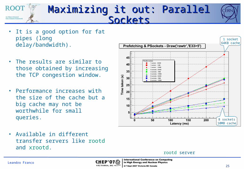
Maximizing it out: Parallel Maximizing it out: Parallel SocketsSockets
8 sockets10MB cache
1 socket64KB cache
rootd server
• It is a good option for fat pipes (long delay/bandwidth).
• The results are similar to those obtained by increasing the TCP congestion window.
• Performance increases with the size of the cache but a big cache may not be worthwhile for small queries.
• Available in different transfer servers like rootd and xrootd.
26Leandro Franco
Current and Future WorkCurrent and Future Work• With this new cache, we were able to try another
improvement: Parallel Unzipping. We can now use a second core to unzip the data in the cache and boost the overall performance.
• We are in close collaboration with Fabrizio Furano (xrootd) to test the new asynchronous readings.• A modified TTreeCache is used and the readv() is replaced by a
bunch of async requests.• The results are encouraging* and we would like to improve it further
with an async readv() request. This would reduce the overhead of normal async reads and allow us to parallelize the work.
• Still some work to do to fine tune the learning phase and file opening (reduce the opening to 2 requests).
• Understand how new technologies like BIC-TCP can improve the slow start.
* Check out Fabrizio’s talk for more details
27Leandro Franco
ConclusionsConclusions• Data analysis can be performed efficiently from remote
locations (even with limited bandwidth like an ADSL connection).
• The extensions have been introduced in:• rootd, http, xrootd(thanks to Fabrizio* and Andy), dCache (from
version 1.7.0-39) and Daniel Engh from Vanderbilt showed interest for IBP (Internet Backbone Protocol).
• In addition to network latency, disk latency is also improved in certain conditions. Specially if this kind of read is done atomically to avoid context switches between processes.
• TCP (and all the its variants seen so far) are optimized for “data transfer”, making “data access” extremely inefficient. More work is needed in collaboration with networking groups to find an efficient way for data access.
• We have to catch up with bandwidth upgrades and change the block sizes according to that (more bandwidth, bigger block transfers and bigger TCP windows).
* Check out Fabrizio’s talk for more details