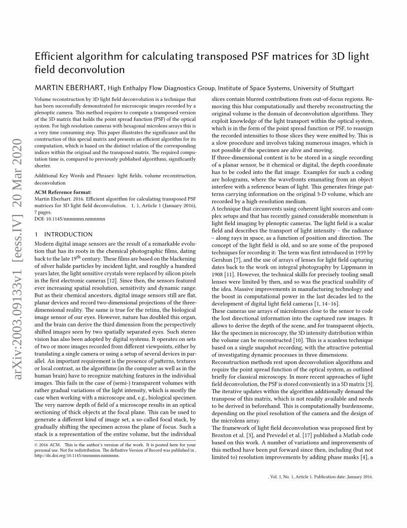
E�icient algorithm for calculating transposed PSF matrices for 3D lightfield deconvolution

MARTIN EBERHART, High Enthalpy Flow Diagnostics Group, Institute of Space Systems, University of Stu�gart

Volume reconstruction by 3D light �eld deconvolution is a technique that

has been successfully demonstrated for microscopic images recorded by a

plenoptic camera. �is method requires to compute a transposed version

of the 5D matrix that holds the point spread function (PSF) of the optical

system. For high resolution cameras with hexagonal microlens arrays this is

a very time consuming step. �is paper illustrates the signi�cance and the

construction of this special matrix and presents an e�cient algorithm for its

computation, which is based on the distinct relation of the corresponding

indices within the original and the transposed matrix. �e required compu-

tation time is, compared to previously published algorithms, signi�cantly

shorter.

Additional Key Words and Phrases: light �elds, volume reconstruction,

deconvolution

ACM Reference format:Martin Eberhart. 2016. E�cient algorithm for calculating transposed PSF

matrices for 3D light �eld deconvolution. 1, 1, Article 1 (January 2016),

7 pages.

DOI: 10.1145/nnnnnnn.nnnnnnn

1 INTRODUCTIONModern digital image sensors are the result of a remarkable evolu-

tion that has its roots in the chemical photographic �lms, dating

back to the late 19th

century. �ese �lms are based on the blackening

of silver halide particles by incident light, and roughly a hundred

years later, the light sensitive crystals were replaced by silicon pixels

in the �rst electronic cameras [12]. Since then, the sensors featured

ever increasing spatial resolution, sensitivity and dynamic range.

But as their chemical ancestors, digital image sensors still are �at,

planar devices and record two-dimensional projections of the three-

dimensional reality. �e same is true for the retina, the biological

image sensor of our eyes. However, nature has doubled this organ,

and the brain can derive the third dimension from the perspectively

shi�ed images seen by two spatially separated eyes. Such stereo

vision has also been adopted by digital systems. It operates on sets

of two or more images recorded from di�erent viewpoints, either by

translating a single camera or using a setup of several devices in par-

allel. An important requirement is the presence of pa�erns, textures

or local contrast, as the algorithms (in the computer as well as in the

human brain) have to recognize matching features in the individual

images. �is fails in the case of (semi-) transparent volumes with

rather gradual variations of the light intensity, which is mostly the

case when working with a microscope and, e.g., biological specimen.

�e very narrow depth of �eld of a microscope results in an optical

sectioning of thick objects at the focal plane. �is can be used to

generate a di�erent kind of image set, a so-called focal stack, by

gradually shi�ing the specimen across the plane of focus. Such a

stack is a representation of the entire volume, but the individual

© 2016 ACM. �is is the author’s version of the work. It is posted here for your

personal use. Not for redistribution. �e de�nitive Version of Record was published in ,

h�p://dx.doi.org/10.1145/nnnnnnn.nnnnnnn.

slices contain blurred contributions from out-of-focus regions. Re-

moving this blur computationally and thereby reconstructing the

original volume is the domain of deconvolution algorithms. �ey

exploit knowledge of the light transport within the optical system,

which is in the form of the point spread function or PSF, to reassign

the recorded intensities to those slices they were emi�ed by. �is is

a slow procedure and involves taking numerous images, which is

not possible if the specimen are alive and moving.

If three-dimensional content is to be stored in a single recording

of a planar sensor, be it chemical or digital, the depth coordinate

has to be coded into the �at image. Examples for such a coding

are holograms, where the wavefronts emanating from an object

interfere with a reference beam of light. �is generates fringe pat-

terns carrying information on the original 3-D volume, which are

recorded by a high-resolution medium.

A technique that circumvents using coherent light sources and com-

plex setups and that has recently gained considerable momentum is

light �eld imaging by plenoptic cameras. �e light �eld is a scalar

�eld and describes the transport of light intensity – the radiance

– along rays in space, as a function of position and direction. �e

concept of the light �eld is old, and so are some of the proposed

techniques for recording it: �e term was �rst introduced in 1939 by

Gershun [7], and the use of arrays of lenses for light �eld capturing

dates back to the work on integral photography by Lippmann in

1908 [11]. However, the technical skills for precisely tooling small

lenses were limited by then, and so was the practical usability of

the idea. Massive improvements in manufacturing technology and

the boost in computational power in the last decades led to the

development of digital light �eld cameras [1, 14–16].

�ese cameras use arrays of microlenses close to the sensor to code

the lost directional information into the captured raw images. It

allows to derive the depth of the scene, and for transparent objects,

like the specimen in microscopy, the 3D intensity distribution within

the volume can be reconstructed [10]. �is is a scanless technique

based on a single snapshot recording, with the a�ractive potential

of investigating dynamic processes in three dimensions.

Reconstruction methods rest upon deconvolution algorithms and

require the point spread function of the optical system, as outlined

brie�y for classical microscopy. In more recent approaches of light

�eld deconvolution, the PSF is stored conveniently in a 5D matrix [3].

�e iterative updates within the algorithm additionally demand the

transpose of this matrix, which is not readily available and needs

to be derived in beforehand. �is is computationally burdensome,

depending on the pixel resolution of the camera and the design of

the microlens array.

�e framework of light �eld deconvolution was proposed �rst by

Broxton et al. [3], and Prevedel et al. [17] published a Matlab code

based on this work. A number of variations and improvements of

this method have been put forward since then, including (but not

limited to) resolution improvements by adding phase masks [4], a

, Vol. 1, No. 1, Article 1. Publication date: January 2016.

arX

iv:2

003.

0913

3v1

[ee

ss.I

V]

20

Mar

202

0

1:2 • Eberhart et al.

reconstruction in the phase-space domain with reduced artifacts

and considerable speed-up [13] and improved reconstruction quality

by incorporating depth-dependant �ltering in the deconvolution

algorithm [19]. While the theory of light �eld capturing, the design

of the optical setups and the proposed reconstruction algorithms

are presented in great detail in the literature, the reader is le� alone

with the structure of the transposed PSF matrix and how to compute

it.

�e contribution of this paper is two-fold: First, we clarify the sig-

ni�cance of this matrix and its relation to the original PSF, and

complement this by hints on how to record a light �eld PSF ex-

perimentally in a suitable matrix structure. Second, we present

an e�cient and fast algorithm for computing the transposed PSF

matrix.

2 LIGHT FIELD IMAGING AND VOLUMERECONSTRUCTION

In a standard photographic camera, single pixels of the sensor (or

the grains of a chemical �lm) integrate the incident light over a

certain solid angle. As a consequence, the directional information

is lost and the captured images are �at. In a plenoptic light �eld

camera, on the other hand, an additional microlens array is inserted

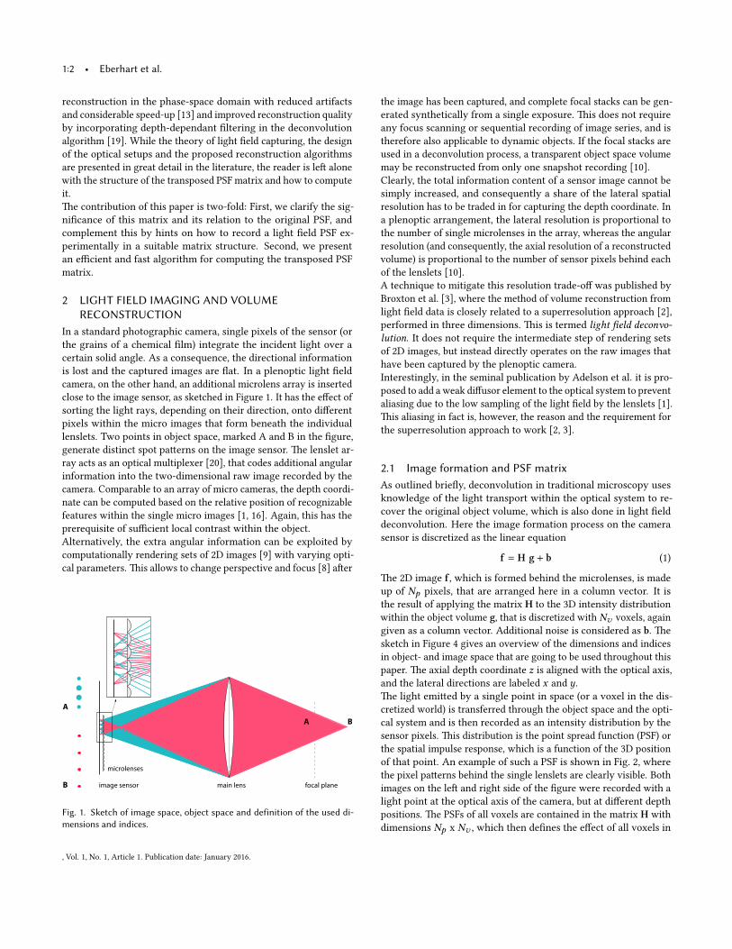
close to the image sensor, as sketched in Figure 1. It has the e�ect of

sorting the light rays, depending on their direction, onto di�erent

pixels within the micro images that form beneath the individual

lenslets. Two points in object space, marked A and B in the �gure,

generate distinct spot pa�erns on the image sensor. �e lenslet ar-

ray acts as an optical multiplexer [20], that codes additional angular

information into the two-dimensional raw image recorded by the

camera. Comparable to an array of micro cameras, the depth coordi-

nate can be computed based on the relative position of recognizable

features within the single micro images [1, 16]. Again, this has the

prerequisite of su�cient local contrast within the object.

Alternatively, the extra angular information can be exploited by

computationally rendering sets of 2D images [9] with varying opti-

cal parameters. �is allows to change perspective and focus [8] a�er

image sensor

microlenses

main lens focal plane

B

B

A

A

Fig. 1. Sketch of image space, object space and definition of the used di-mensions and indices.

the image has been captured, and complete focal stacks can be gen-

erated synthetically from a single exposure. �is does not require

any focus scanning or sequential recording of image series, and is

therefore also applicable to dynamic objects. If the focal stacks are

used in a deconvolution process, a transparent object space volume

may be reconstructed from only one snapshot recording [10].

Clearly, the total information content of a sensor image cannot be

simply increased, and consequently a share of the lateral spatial

resolution has to be traded in for capturing the depth coordinate. In

a plenoptic arrangement, the lateral resolution is proportional to

the number of single microlenses in the array, whereas the angular

resolution (and consequently, the axial resolution of a reconstructed

volume) is proportional to the number of sensor pixels behind each

of the lenslets [10].

A technique to mitigate this resolution trade-o� was published by

Broxton et al. [3], where the method of volume reconstruction from

light �eld data is closely related to a superresolution approach [2],

performed in three dimensions. �is is termed light �eld deconvo-lution. It does not require the intermediate step of rendering sets

of 2D images, but instead directly operates on the raw images that

have been captured by the plenoptic camera.

Interestingly, in the seminal publication by Adelson et al. it is pro-

posed to add a weak di�usor element to the optical system to prevent

aliasing due to the low sampling of the light �eld by the lenslets [1].

�is aliasing in fact is, however, the reason and the requirement for

the superresolution approach to work [2, 3].

2.1 Image formation and PSF matrixAs outlined brie�y, deconvolution in traditional microscopy uses

knowledge of the light transport within the optical system to re-

cover the original object volume, which is also done in light �eld

deconvolution. Here the image formation process on the camera

sensor is discretized as the linear equation

f = H g + b (1)

�e 2D image f , which is formed behind the microlenses, is made

up of Np pixels, that are arranged here in a column vector. It is

the result of applying the matrix H to the 3D intensity distribution

within the object volume g, that is discretized with Nv voxels, again

given as a column vector. Additional noise is considered as b. �e

sketch in Figure 4 gives an overview of the dimensions and indices

in object- and image space that are going to be used throughout this

paper. �e axial depth coordinate z is aligned with the optical axis,

and the lateral directions are labeled x and y.

�e light emi�ed by a single point in space (or a voxel in the dis-

cretized world) is transferred through the object space and the opti-

cal system and is then recorded as an intensity distribution by the

sensor pixels. �is distribution is the point spread function (PSF) or

the spatial impulse response, which is a function of the 3D position

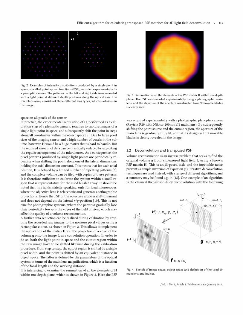
of that point. An example of such a PSF is shown in Fig. 2, where

the pixel pa�erns behind the single lenslets are clearly visible. Both

images on the le� and right side of the �gure were recorded with a

light point at the optical axis of the camera, but at di�erent depth

positions. �e PSFs of all voxels are contained in the matrix H with

dimensions Np x Nv , which then de�nes the e�ect of all voxels in

, Vol. 1, No. 1, Article 1. Publication date: January 2016.

E�icient algorithm for calculating transposed PSF matrices for 3D light field deconvolution • 1:3

Fig. 2. Examples of intensity distributions produced by a single point inspace, so-called point spread functions (PSF), recorded experimentally bya plenoptic camera. The pa�erns on the le� and right side were recordedwith a light point at di�erent depth positions along the optical axis. Themicrolens array consists of three di�erent lens types, which is obvious inthe image.

space on all pixels of the sensor.

In practice, the experimental acquisition of H, performed as a cali-

bration step of a plenoptic camera, requires to capture images of a

single light point in space, and subsequently shi� the point in steps

along all coordinates within the object space [5]. Due to large pixel

sizes of the imaging sensor and a high number of voxels in the vol-

ume, however, H would be a huge matrix that is hard to handle. But

the required amount of data can be drastically reduced by exploiting

the regular arrangement of the microlenses. As a consequence, the

pixel pa�erns produced by single light points are periodically re-

peating when shi�ing the point along one of the lateral dimensions,

holding the axial dimension constant. �is means that for each axial

position, H is de�ned by a limited number of repeating pa�erns [3],

and the complete volume can be tiled with copies of these pa�erns.

It is therefore su�cient to calibrate the system within a small re-

gion that is representative for the used lenslet array. It should be

noted that this holds, strictly speaking, only for ideal microscopes,

where the objective lens is telecentric and generates orthographic

projections. Hence the PSF of the objective alone is shi�-invariant

and does not depend on the lateral x/y-position [10]. �is is not

true for photographic systems, where the pa�erns gradually lose

their periodicity towards the edges of the �eld of view, which may

a�ect the quality of a volume reconstruction.

A further data reduction can be realized during calibration by crop-

ping the recorded raw images to the nonzero pixel values using a

rectangular cutout, as shown in Figure 2. �is allows to implement

the application of the matrix H, i.e. the projection of a voxel of the

volume g onto the image f , as a convolution operation. In order to

do so, both the light point in space and the cutout region within

the raw image have to be shi�ed likewise during the calibration

procedure. From step to step, the cutout region is shi�ed by a single

pixel width, and the point is shi�ed by an equivalent distance in

object space. �e la�er is de�ned by the parameters of the optical

system in terms of the main lens magni�cation, which is a function

of the focal length and the working distance.

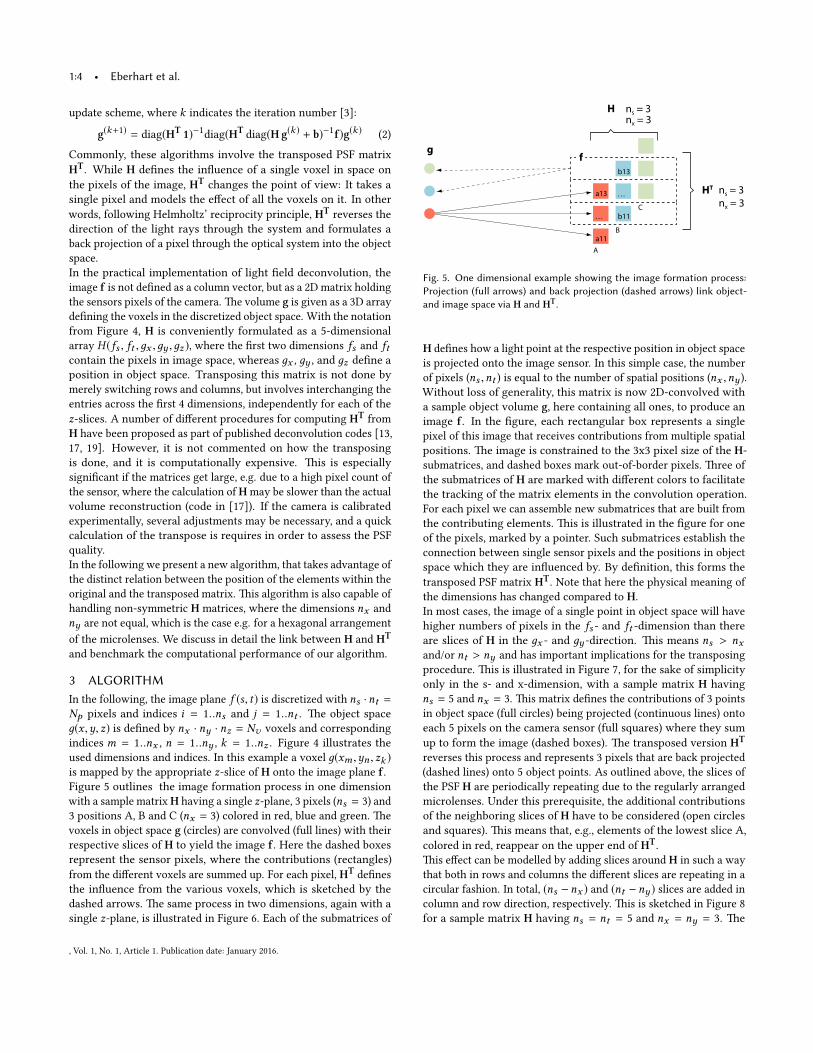
It is interesting to examine the summation of all the elements of Hwithin one depth plane, which is shown in Figure 3. Here the PSF

Fig. 3. Summation of all the elements of the PSF matrix H within one depthplane. The PSF was recorded experimentally using a photographic mainlens, and the structure of the aperture constructed from 9 movable bladesis clearly seen.

was acquired experimentally with a photographic plenoptic camera

(Raytrix R29 with Nikkor 200mm f/4 main lens). By subsequently

shi�ing the point source and the cutout region, the aperture of the

main lens is gradually fully lit, so that its design with 9 movable

blades is clearly revealed in the image.

2.2 Deconvolution and transposed PSFVolume reconstruction is an inverse problem that seeks to �nd the

original volume g from a measured light �eld f , using a known

PSF matrix H. �is is an ill-posed task, and the inevitable noise

prevents a simple inversion of Equation (1). Iterative deconvolution

techniques are used instead, with a range of di�erent algorithms, and

a summary may be found e.g. in [18]. One example of an algorithm

is the classical Richardson-Lucy deconvolution with the following

st

x

y

z

f

g

i=1..ns

j=1..nt

m=1..nx

k=1..nz

g(xm

, yn

, zk )

H( : , : , xm

, yn , z

k )

ns . n

t = N

p

nx

. ny

. nz = N

v

Fig. 4. Sketch of image space, object space and definition of the used di-mensions and indices.

, Vol. 1, No. 1, Article 1. Publication date: January 2016.

1:4 • Eberhart et al.

update scheme, where k indicates the iteration number [3]:

g(k+1) = diag(HT 1)−1diag(HT

diag(Hg(k ) + b)−1f)g(k ) (2)

Commonly, these algorithms involve the transposed PSF matrix

HT. While H de�nes the in�uence of a single voxel in space on

the pixels of the image, HTchanges the point of view: It takes a

single pixel and models the e�ect of all the voxels on it. In other

words, following Helmholtz’ reciprocity principle, HTreverses the

direction of the light rays through the system and formulates a

back projection of a pixel through the optical system into the object

space.

In the practical implementation of light �eld deconvolution, the

image f is not de�ned as a column vector, but as a 2D matrix holding

the sensors pixels of the camera. �e volume g is given as a 3D array

de�ning the voxels in the discretized object space. With the notation

from Figure 4, H is conveniently formulated as a 5-dimensional

array H (fs , ft ,дx ,дy ,дz ), where the �rst two dimensions fs and ftcontain the pixels in image space, whereas дx , дy , and дz de�ne a

position in object space. Transposing this matrix is not done by

merely switching rows and columns, but involves interchanging the

entries across the �rst 4 dimensions, independently for each of the

z-slices. A number of di�erent procedures for computing HTfrom

H have been proposed as part of published deconvolution codes [13,

17, 19]. However, it is not commented on how the transposing

is done, and it is computationally expensive. �is is especially

signi�cant if the matrices get large, e.g. due to a high pixel count of

the sensor, where the calculation of H may be slower than the actual

volume reconstruction (code in [17]). If the camera is calibrated

experimentally, several adjustments may be necessary, and a quick

calculation of the transpose is requires in order to assess the PSF

quality.

In the following we present a new algorithm, that takes advantage of

the distinct relation between the position of the elements within the

original and the transposed matrix. �is algorithm is also capable of

handling non-symmetric H matrices, where the dimensions nx and

ny are not equal, which is the case e.g. for a hexagonal arrangement

of the microlenses. We discuss in detail the link between H and HT

and benchmark the computational performance of our algorithm.

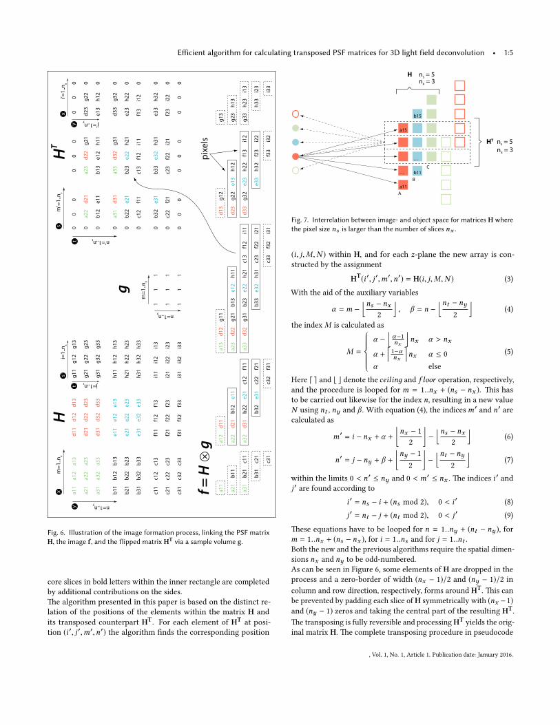
3 ALGORITHMIn the following, the image plane f (s, t) is discretized with ns ·nt =Np pixels and indices i = 1..ns and j = 1..nt . �e object space

д(x ,y, z) is de�ned by nx · ny · nz = Nv voxels and corresponding

indices m = 1..nx , n = 1..ny , k = 1..nz . Figure 4 illustrates the

used dimensions and indices. In this example a voxel д(xm ,yn , zk )is mapped by the appropriate z-slice of H onto the image plane f .Figure 5 outlines the image formation process in one dimension

with a sample matrix H having a single z-plane, 3 pixels (ns = 3) and

3 positions A, B and C (nx = 3) colored in red, blue and green. �e

voxels in object space g (circles) are convolved (full lines) with their

respective slices of H to yield the image f . Here the dashed boxes

represent the sensor pixels, where the contributions (rectangles)

from the di�erent voxels are summed up. For each pixel, HTde�nes

the in�uence from the various voxels, which is sketched by the

dashed arrows. �e same process in two dimensions, again with a

single z-plane, is illustrated in Figure 6. Each of the submatrices of

ns = 3nx = 3

H

HT ns = 3nx = 3

gf

a11

a13

. . . b11

b13

. . .

A

B

C

Fig. 5. One dimensional example showing the image formation process:Projection (full arrows) and back projection (dashed arrows) link object-and image space via H and HT.

H de�nes how a light point at the respective position in object space

is projected onto the image sensor. In this simple case, the number

of pixels (ns ,nt ) is equal to the number of spatial positions (nx ,ny ).

Without loss of generality, this matrix is now 2D-convolved with

a sample object volume g, here containing all ones, to produce an

image f . In the �gure, each rectangular box represents a single

pixel of this image that receives contributions from multiple spatial

positions. �e image is constrained to the 3x3 pixel size of the H-

submatrices, and dashed boxes mark out-of-border pixels. �ree of

the submatrices of H are marked with di�erent colors to facilitate

the tracking of the matrix elements in the convolution operation.

For each pixel we can assemble new submatrices that are built from

the contributing elements. �is is illustrated in the �gure for one

of the pixels, marked by a pointer. Such submatrices establish the

connection between single sensor pixels and the positions in object

space which they are in�uenced by. By de�nition, this forms the

transposed PSF matrix HT. Note that here the physical meaning of

the dimensions has changed compared to H.

In most cases, the image of a single point in object space will have

higher numbers of pixels in the fs - and ft -dimension than there

are slices of H in the дx - and дy -direction. �is means ns > nxand/or nt > ny and has important implications for the transposing

procedure. �is is illustrated in Figure 7, for the sake of simplicity

only in the s- and x-dimension, with a sample matrix H having

ns = 5 and nx = 3. �is matrix de�nes the contributions of 3 points

in object space (full circles) being projected (continuous lines) onto

each 5 pixels on the camera sensor (full squares) where they sum

up to form the image (dashed boxes). �e transposed version HT

reverses this process and represents 3 pixels that are back projected

(dashed lines) onto 5 object points. As outlined above, the slices of

the PSF H are periodically repeating due to the regularly arranged

microlenses. Under this prerequisite, the additional contributions

of the neighboring slices of H have to be considered (open circles

and squares). �is means that, e.g., elements of the lowest slice A,

colored in red, reappear on the upper end of HT.

�is e�ect can be modelled by adding slices around H in such a way

that both in rows and columns the di�erent slices are repeating in a

circular fashion. In total, (ns − nx ) and (nt − ny ) slices are added in

column and row direction, respectively. �is is sketched in Figure 8

for a sample matrix H having ns = nt = 5 and nx = ny = 3. �e

, Vol. 1, No. 1, Article 1. Publication date: January 2016.

E�icient algorithm for calculating transposed PSF matrices for 3D light field deconvolution • 1:5

g11

g12

g13

g11

g12

g13

g21

g22

g23

b11

b12

g21

b13

h11

g22

h12

g23

h13

g31

g32

g33

b21

c11

b22

c12

f11

g31

b23

h21

c13

f12

i11

g32

h22

f13

i12

g33

h23

i13

b31

c21

b32

c22

f21

b33

h31

c23

f22

i21

h32

f23

i22

h33

i23

b11

b12

b13

h11

h12

h13

c31

c32

f31

c33

f32

i31

f33

i32

i33

b21

b22

b23

h21

h22

h23

b31

b32

b33

h31

h32

h33

c11

c12

c13

f11

f12

f13

i11

i12

i13

c21

c22

c23

f21

f22

f23

i21

i22

i23

c31

c32

c33

f31

f32

f33

i31

i32

i33

11

1

11

1

11

1

i=1.

.ns

0 0

0 0

0 0

0 0

0

0g2

1d2

3g2

2 0

0b1

2e1

1b1

3e1

2h1

1e1

3h1

2 0

0

a11

a11

a12

a13

a12

a13

a21

a22

a23

a21

a22

a23

a31

a32

a33

a31

a32

a33

a22

a23

a31

a33

d11

d12

d13

d11

d12

d13

d21

d22

d23

d21

d22

d23

d31

d32

d33

d31

d32

d33

d21

d22

d31

d32

g31

d33

g32

0

0b2

2b2

3h2

1e2

3h2

2 0

0c1

2f1

1c1

3f1

2i1

1f1

3i1

2 0

0b3

2b3

3

e11

e12

e13

e21

e22

e23

e31

e32

e33

e11

e12

e13

e21

e22

e23

e31

e32

e33

e21

e22

e31

e32

h31

e33

h32

0

0c2

2f2

1c2

3f2

2i2

1f2

3i2

2 0

0 0

0 0

0 0

0 0

0

j=1..nt

m=1

..nx

n=1..ny

s

t

x

y

i’=1.

.nx

j’=1..ny

m’=

1..n

s

n’=1..nt

x

y

s

t

HT

H

g

f = H

g×

pixe

ls

m=1

..nx

n=1..ny

Fig. 6. Illustration of the image formation process, linking the PSF matrixH, the image f , and the flipped matrix HT via a sample volume g.

core slices in bold le�ers within the inner rectangle are completed

by additional contributions on the sides.

�e algorithm presented in this paper is based on the distinct re-

lation of the positions of the elements within the matrix H and

its transposed counterpart HT. For each element of HT

at posi-

tion (i ′, j ′,m′,n′) the algorithm �nds the corresponding position

ns = 5nx = 3

H

HT ns = 5nx = 3

a11

a15

. . . b11

b15

. . .

A

B

C

Fig. 7. Interrelation between image- and object space for matrices H wherethe pixel size ns is larger than the number of slices nx .

(i, j,M,N ) within H, and for each z-plane the new array is con-

structed by the assignment

HT(i ′, j ′,m′,n′) = H(i, j,M,N ) (3)

With the aid of the auxiliary variables

α =m −⌊ns − nx

2

⌋, β = n −

⌊nt − ny2

⌋(4)

the index M is calculated as

M =

α −

⌊α−1

nx

⌋nx α > nx

α +⌈

1−αnx

⌉nx α ≤ 0

α else

(5)

Here d e and b c denote the ceilinд and f loor operation, respectively,

and the procedure is looped for m = 1..nx + (ns − nx ). �is has

to be carried out likewise for the index n, resulting in a new value

N using nt , ny and β . With equation (4), the indicesm′ and n′ are

calculated as

m′ = i − nx + α +⌊nx − 1

2

⌋−

⌊ns − nx2

⌋(6)

n′ = j − ny + β +⌊ny − 1

2

⌋−

⌊nt − ny2

⌋(7)

within the limits 0 < n′ ≤ ny and 0 < m′ ≤ nx . �e indices i ′ and

j ′ are found according to

i ′ = ns − i + (ns mod 2), 0 < i ′ (8)

j ′ = nt − j + (nt mod 2), 0 < j ′ (9)

�ese equations have to be looped for n = 1..ny + (nt − ny ), for

m = 1..nx + (ns − nx ), for i = 1..ns and for j = 1..nt .

Both the new and the previous algorithms require the spatial dimen-

sions nx and ny to be odd-numbered.

As can be seen in Figure 6, some elements of H are dropped in the

process and a zero-border of width (nx − 1)/2 and (ny − 1)/2 in

column and row direction, respectively, forms around HT. �is can

be prevented by padding each slice of H symmetrically with (nx −1)and (ny − 1) zeros and taking the central part of the resulting HT

.

�e transposing is fully reversible and processing HTyields the orig-

inal matrix H. �e complete transposing procedure in pseudocode

, Vol. 1, No. 1, Article 1. Publication date: January 2016.

1:6 • Eberhart et al.

I

H

G

I

G

C

B

A

C

A

I

H

G

I

G

F

E

D

F

D

C

B

A

C

A

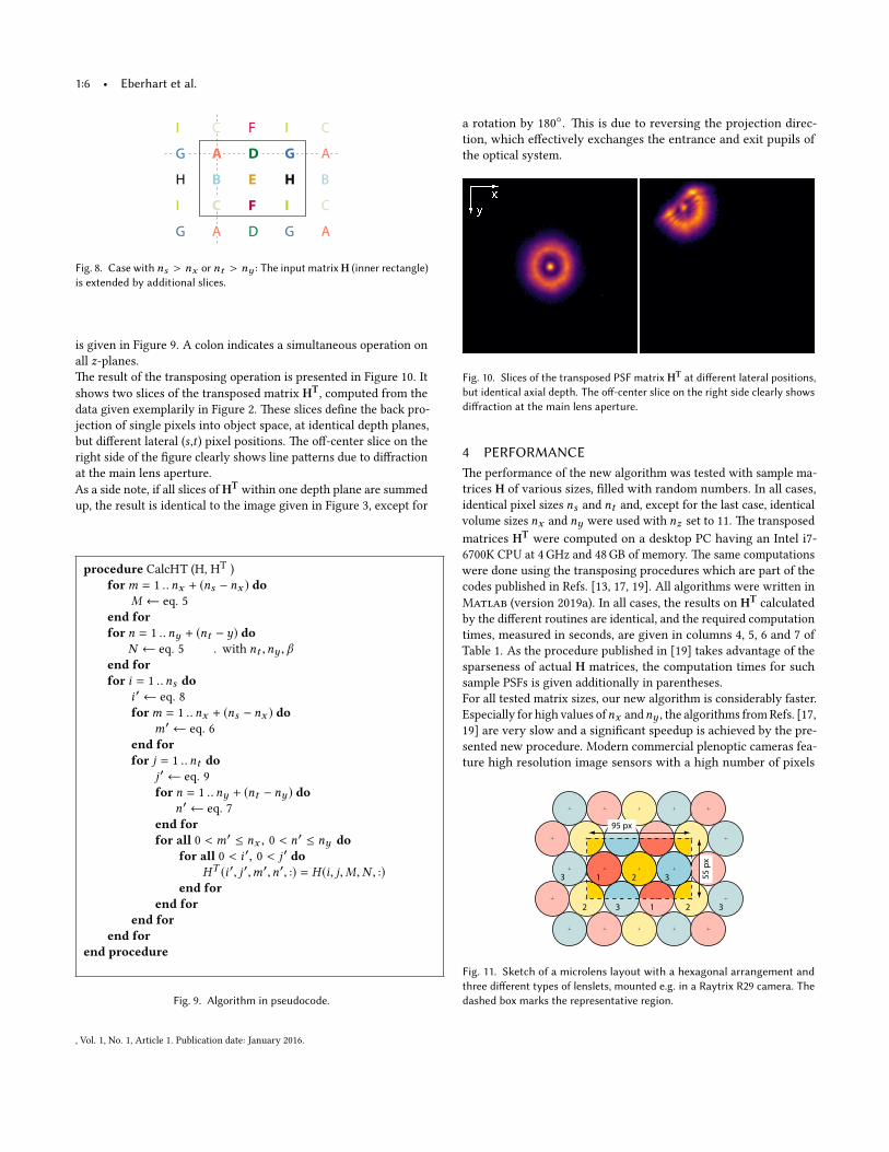
Fig. 8. Case with ns > nx or nt > ny : The input matrixH (inner rectangle)is extended by additional slices.

is given in Figure 9. A colon indicates a simultaneous operation on

all z-planes.

�e result of the transposing operation is presented in Figure 10. It

shows two slices of the transposed matrix HT, computed from the

data given exemplarily in Figure 2. �ese slices de�ne the back pro-

jection of single pixels into object space, at identical depth planes,

but di�erent lateral (s ,t ) pixel positions. �e o�-center slice on the

right side of the �gure clearly shows line pa�erns due to di�raction

at the main lens aperture.

As a side note, if all slices of HTwithin one depth plane are summed

up, the result is identical to the image given in Figure 3, except for

procedure CalcHT (H, HT

)

form = 1 ..nx + (ns − nx ) doM ← eq. 5

end forfor n = 1 ..ny + (nt − y) do

N ← eq. 5 . with nt ,ny , βend forfor i = 1 ..ns do

i ′ ← eq. 8

form = 1 ..nx + (ns − nx ) dom′ ← eq. 6

end forfor j = 1 ..nt do

j ′ ← eq. 9

for n = 1 ..ny + (nt − ny ) don′ ← eq. 7

end forfor all 0 < m′ ≤ nx , 0 < n′ ≤ ny do

for all 0 < i ′, 0 < j ′ doHT (i ′, j ′,m′,n′, :) = H (i, j,M,N , :)

end forend for

end forend for

end procedure

Fig. 9. Algorithm in pseudocode.

a rotation by 180◦. �is is due to reversing the projection direc-

tion, which e�ectively exchanges the entrance and exit pupils of

the optical system.

Fig. 10. Slices of the transposed PSF matrix HT at di�erent lateral positions,but identical axial depth. The o�-center slice on the right side clearly showsdi�raction at the main lens aperture.

4 PERFORMANCE�e performance of the new algorithm was tested with sample ma-

trices H of various sizes, �lled with random numbers. In all cases,

identical pixel sizes ns and nt and, except for the last case, identical

volume sizes nx and ny were used with nz set to 11. �e transposed

matrices HTwere computed on a desktop PC having an Intel i7-

6700K CPU at 4 GHz and 48 GB of memory. �e same computations

were done using the transposing procedures which are part of the

codes published in Refs. [13, 17, 19]. All algorithms were wri�en in

Matlab (version 2019a). In all cases, the results on HTcalculated

by the di�erent routines are identical, and the required computation

times, measured in seconds, are given in columns 4, 5, 6 and 7 of

Table 1. As the procedure published in [19] takes advantage of the

sparseness of actual H matrices, the computation times for such

sample PSFs is given additionally in parentheses.

For all tested matrix sizes, our new algorithm is considerably faster.

Especially for high values ofnx andny , the algorithms from Refs. [17,

19] are very slow and a signi�cant speedup is achieved by the pre-

sented new procedure. Modern commercial plenoptic cameras fea-

ture high resolution image sensors with a high number of pixels

1 2 3

2 3 1 2 3

3 1 2 3

2 3 1 2

95 px

55 p

x

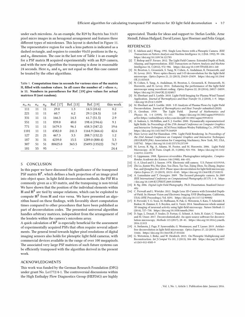
Fig. 11. Sketch of a microlens layout with a hexagonal arrangement andthree di�erent types of lenslets, mounted e.g. in a Raytrix R29 camera. Thedashed box marks the representative region.

, Vol. 1, No. 1, Article 1. Publication date: January 2016.

E�icient algorithm for calculating transposed PSF matrices for 3D light field deconvolution • 1:7

under each microlens. As an example, the R29 by Raytrix has 31x31

pixel micro images in an hexagonal arrangement and features three

di�erent types of microlenses. �is layout is sketched in Figure 11.

�e representative region for such a lens pa�ern is indicated as a

dashed rectangle, and requires to consider 95x55 positions in the nxand ny dimension. �e case in the last row of Table 1 is an example

for a PSF matrix H acquired experimentally with an R29 camera,

and with the new algorithm the transposing is done in reasonable

24 seconds. Here nx and ny are not equal so that this case cannot

be treated by the other algorithms.

Table 1. Computation time in seconds for various sizes of the matrixH, �lled with random values. In all cases the number of z-slices nzis 11. Numbers in parentheses for Ref. [19] give values for actualmatrices H (not random).

ns ,nt nx ny Ref. [17] Ref. [13] Ref. [19] this work

111 11 11 29.0 1.3 14.5 (10.6) 0.2

221 11 11 60.7 6.2 29.1 (24.5) 1.0

331 11 11 166.3 14.3 61.7 (51.5) 2.9

551 11 11 839.0 48.0 198.4 (194.6) 9.1

771 11 11 1679.3 96.1 658.3 (347.2) 19.6

1101 11 11 4382.0 241.3 1164.9 (466.6) 42.6

127 21 21 467.3 3.5 208.7 (152.2) 1.2

187 31 31 4239.0 15.5 1289.0 (880.4) 5.3

307 51 51 88425.0 363.5 25493 (13522) 74.7

181 55 95 - - - 24.4

5 CONCLUSIONIn this paper we have discussed the signi�cance of the transposed

PSF matrix HT, which de�nes a back projection of an image pixel

into object space. In light �eld deconvolution methods, the PSF H is

commonly given as a 5D matrix, and the transposing is non-trivial.

We have shown that the position of the individual elements within

H and HTare tied by unique relations, which can be exploited to

compute HTfrom H and vice versa. We have presented an algo-

rithm based on these �ndings, with favorably short computation

times compared to other procedures that have been published as

part of deconvolution codes. �e presented universal algorithm

handles arbitrary matrices, independent from the arrangement of

the lenslets within the camera’s microlens array.

A quick calculation of HTis especially bene�cial for the assessment

of experimentally acquired PSFs that o�en require several adjust-

ments. �e general trend towards higher pixel resolutions of digital

imaging sensors also holds for plenoptic light �eld cameras, with

commercial devices available in the range of over 100 megapixels.

�e associated very large PSF matrices of such future systems can

be e�ciently transposed with the algorithm derived in the present

work.

ACKNOWLEDGMENTS�is work was funded by the German Research Foundation (DFG)

under grant No. Lo1772/4-1. �e controversial discussions within

the High Enthalpy Flow Diagnostics Group (HEFDiG) are highly

appreciated. �anks for ideas and support to: Stefan Loehle, Arne

Meindl, Fabian Hufgard, David Leiser, Igor Hoerner and Felix Grigat.

REFERENCES[1] E. Adelson and J. Wang. 1992. Single Lens Stereo with a Plenoptic Camera. IEEE

Transactions on Pa�ern Analysis and Machine Intelligence 14, 2 (Feb. 1992), 99–106.

h�ps://doi.org/10.1109/34.121783

[2] T. Bishop and P. Favaro. 2012. �e Light Field Camera: Extended Depth of Field,

Aliasing, and Superresolution. IEEE Transactions on Pa�ern Analysis and MachineIntelligence 34, 5 (2012), 972–986. h�ps://doi.org/10.1109/TPAMI.2011.168

[3] M. Broxton, L. Grosenick, S. Yang, N. Cohen, A. Andalman, K. Deisseroth, and

M. Levoy. 2013. Wave optics theory and 3-D deconvolution for the light �eld

microscope. Optics Express 21, 21 (2013), 25418–25439. h�ps://doi.org/10.1364/

OE.21.025418

[4] N. Cohen, S. Yang, A. Andalman, M. Broxton, L. Grosenick, K. Deisseroth, M.

Horowitz, and M. Levoy. 2014. Enhancing the performance of the light �eld

microscope using wavefront coding. Optics Express 22, 20 (2014), 24817–24839.

h�ps://doi.org/10.1364/OE.22.024817

[5] M. Eberhart and S. Loehle. 2018. Light-Field Imaging for Plasma Wind Tunnel

Application. Journal of �ermophysics and Heat Transfer 33, 2 (2018), 1–9. h�ps:

//doi.org/10.2514/1.t5499

[6] M. Eberhart and S. Loehle. 2020. 3-D Analysis of Plasma Flows by Light Field

Deconvolution. Journal of �ermophysics and Heat Transfer submi�ed (2020).

[7] A. Gershun. 1939. �e Light Field. Journal of Mathematics andPhysics 18, 1-4 (1939), 51–151. h�ps://doi.org/10.1002/sapm193918151

arXiv:h�ps://onlinelibrary.wiley.com/doi/pdf/10.1002/sapm193918151

[8] A. Isaksen, L. McMillan, and S. J. Gortler. 2000. Dynamically reparameterized

light �elds. In Proceedings of the 27th Annual Conference on Computer Graphicsand Interactive Techniques. ACM Press/Addison-Wesley Publishing Co., 297��306.

h�ps://doi.org/10.1145/344779.344929

[9] Marc Levoy and Pat Hanrahan. 1996. Light Field Rendering. In Proceedings ofthe 23rd Annual Conference on Computer Graphics and Interactive Techniques(SIGGRAPH �96). Association for Computing Machinery, New York, NY, USA,

31��42. h�ps://doi.org/10.1145/237170.237199

[10] M. Levoy, R. Ng, A. Adams, M. Footer, and M. Horowitz. 2006. Light Field

Microscopy. ACM Trans. Graph. 25, 3 (2006), 924–934. h�ps://doi.org/10.1145/

1141911.1141976

[11] G. Lippmann. 1908. Epreuves reversibles. Photographies integrales. Comptes-Rendus Academie des Sciences 146 (1908), 446–451.

[12] G. A. Lloyd and S. J. Sasson. 1978. Electronic still camera. U.S. Patent 4131919A.

[13] Zhi Lu, Jiamin Wu, Hui Qiao, You Zhou, Tao Yan, Zijing Zhou, Xu Zhang, Jingtao

Fan, and Qionghai Dai. 2019. Phase-space deconvolution for light �eld microscopy.

Optics Express 27, 13 (2019), 18131–8145. h�ps://doi.org/10.1364/OE.27.018131

[14] A. Lumsdaine and T. Georgiev. 2009. �e focused plenoptic camera. In 2009IEEE International Conference on Computational Photography (ICCP). 1–8. h�ps:

//doi.org/10.1109/ICCPHOT.2009.5559008

[15] R. Ng. 2006. Digital Light Field Photography. Ph.D. Dissertation. Stanford Univer-

sity.

[16] C. Perwaß and L. Wietzke. 2012. Single Lens 3D-Camera with Extended Depth-

of-Field. In Human Vision and Electronic Imaging XVII (Burlingame, California,

USA) (SPIE Proceedings), Vol. 8291. h�ps://doi.org/10.1117/12.909882

[17] R. Prevedel, Y. G. Yoon, M. Ho�mann, N. Pak, G. Wetzstein, S. Kato, T. Schrodel, R.

Raskar, M. Zimmer, E. S. Boyden, and A. Vaziri. 2014. Simultaneous whole-animal

3D imaging of neuronal activity using light-�eld microscopy. Nature Methods 11

(2014), 727–730. h�ps://doi.org/10.1038/nmeth.2964

[18] D. Sage, L. Donati, F. Soulez, D. Fortun, G. Schmit, A. Seitz, R. Guiet, C. Vonesch,

and M. Unser. 2017. DeconvolutionLab2: An open-source so�ware for deconvo-

lution microscopy. Methods 115 (2017), 28–41. h�ps://doi.org/10.1016/j.ymeth.

2016.12.015

[19] A. Stefanoiu, J. Page, P. Symvoulidis, G. Westmeyer, and T. Lasser. 2019. Artifact-

free deconvolution in light �eld microscopy. Optics Express 27, 22 (2019), 31644–

31666. h�ps://doi.org/10.1364/OE.27.031644

[20] G. Wetzstein, I. Ihrke, and W. Heidrich. 2013. On Plenoptic Multiplexing and

Reconstruction. Int J Comput Vis 101, 2 (2013), 384–400. h�ps://doi.org/10.1007/

s11263-012-0585-9

, Vol. 1, No. 1, Article 1. Publication date: January 2016.