Behav Res (2016) 48:42–52DOI 10.3758/s13428-014-0558-8

Efficient estimation of Weber’s W

Steven T. Piantadosi1

Published online: 27 June 2015© Psychonomic Society, Inc. 2015

Abstract Many studies rely on estimation of Weber ratios(W ) in order to quantify the acuity an individual’s approxi-mate number system. This paper discusses several problemsencountered in estimating W using the standard methods,most notably low power and inefficiency. Through simu-lation, this work shows that W can best be estimated in aBayesian framework that uses an inverse (1/W ) prior. Thisbeneficially balances a bias/variance trade-off and, whenused with MAP estimation is extremely simple to imple-ment. Use of this scheme substantially improves statisticalpower in examining correlates of W .

Keywords Numerical cognition · Statistical estimation ·Weber ratio · Bayesian statistics

A common task in the study of numerical cognition isestimating the acuity of the approximate number system(Dehaene, 1997). This system is active in representingand comparing numerical magnitudes that are too large toexactly count. A typical kind of stimulus is shown in Fig. 1,where participants might be asked to determine if there aremore red or black dots, but the total area, minimum, and

� Steven T. Piantadosispiantado@gmail.com

1 Department of Brain and Cognitive Sciences, Universityof Rochester,Rochester, NY, USA

maximum sizes of these colored dots are equal, encour-aging participants to use number rather than these othercorrelated dimensions to complete the comparison.1 In thisdomain, human performance follows Weber’s law, a moregeneral psychophysical finding that the just noticeable dif-ference between stimuli scales with their magnitude. Higherintensity stimuli—here, higher numbers—appear to be rep-resented with lower absolute fidelity, but constant fidelityrelative to their magnitude. Since Fechner (1860), somehave characterized the psychological scaling of numbersas logarithmic, with the effective psychological distancebetween representations of numbers n and m scaling asn/m (Dehaene, 1997; Masin et al., 2009; Nieder et al.,2002; Nieder and Miller, 2004; Nieder & Merten, 2007;Nieder & Dehaene, 2009; Portugal & Svaiter, 2011; Sunet al., 2012). Alternatively, others have characterized numer-ical representations with a close but distinct alternative: alinear scale with linearly increasing error (standard devi-ation) on the representations, known as scale variability(Gibbon, 1977; Meck & Church, 1983; Whalen et al., 1999;Gallistel & Gelman, 1992). This latter formalization moti-vates characterizing an individual’s behavior by fitting asingle parameter, W , which determines how the standarddeviation of a representation scales with its magnitude: eachnumerosity n is represented with a standard deviation of W ·n. In tasks where subjects must compare two magnitudes,

1Unfortunately, it is impossible to simultaneously control all othervariables correlated with number. In this example, for instance, themean dot size also varies.

Behav Res (2016) 48:42–52 43

Fig. 1 An example stimulus for an approximate number task whereparticipants must rapidly decide if there are more black or red dots.The areas, minimum sizes, and maximum sizes between the dots arecontrolled, and the dots are intermixed in order to discourage strategiesbased on spatial extent

n1 and n2, this psychophysics can be formalized (Halberda& Feigenson, 2008) by fitting W to their observed accuracyvia,

P(correct | W,n1, n2) = �

⎡⎢⎣ |n1 − n2|

W ·√

n21 + n22

⎤⎥⎦ . (1)

In this equation, � is the cumulative normal distributionfunction. The value in Eq. 1 gives the probability that a sam-ple from a normal distribution centered at n1 with standarddeviation W · n1 will be larger than a sample from a dis-tribution centered at n2 with standard deviation W · n2 (forn1 > n2). The values n1 and n2 are fixed by the experimen-tal design; the observed probability of answering accuratelyis measured behaviorally; and W is treated as a free variablethat characterizes the acuity of the psychophysical system.As W → 0, the standard deviation of each representationgoes to 0, and so accuracy will increase. AsW gets large, thedenominator in Eq. 1 goes to zero and accuracy approachesthe chance rate of 50 %.

The precise value of W for an individual is often treatedas a core measurement of the approximate system’s acuity(Gilmore et al., 2011), and is compellingly related to otherdomains: for instance, it correlates with exact symbolicmath performance (Halberda & Feigenson, 2008; Mussolinet al., 2012; Bonny & Lourenco, 2013), its value changesover development and age (Halberda & Feigenson, 2008;Halberda et al., 2012), and is shared among human groups(Pica et al., 2004; Dehaene et al., 2008; Frank et al., 2008).

Despite the importance of W as a psychophysical quan-tity, little work has examined the most efficient practicesfor estimating it from behavioral data. The present paper

evaluates several different techniques for estimating W inorder to determine which are most efficient. Since the prob-lem of determining W is at its core a statistical inferenceproblem—one of determining a psychophysical variablethat is not directly observable—our approach is framed interms of Bayesian inference. This work draws on Bayesiantools and ways of thinking that have increasingly becomepopular in psychology (Kruschke 2010a, b, c). In the con-text of the approximate number system, the first work toinfer Weber ratios through Bayesian data analysis was Leeand Sarnecka (2010, 2011), who showed that children’sperformance in number tasks is better described by dis-crete and exact knower-level theories than ones based in theapproximate number system.

With a Bayesian framing, we are interested in P(W | D),the probability that any value for W is the true one, givensome observed behavioral data D. By Bayes rule, this canbe found via P(W | D) ∝ P(D | W) · P(W), whereP(D | W) is the likelihood of the data given a partic-ular W and P(W) is a prior expectation about what W

are likely. In fact, P(D | W) is already well establishedin the literature: the likelihood W assigns to the data canbe found with Eq. 1, which quantifies the probability thata subject would answer correctly on each given trial forany choice of W .2 The key additional part to the Bayesiansetting is therefore the prior P(W), which is classically aquantification of our expectations about W before any datais observed.

The choice of P(W) presents a clear challenge. Thereare many qualitatively different priors that one might chooseand, in this case, no clear theoretical reasons for preferringone over another. These types of priors include those thatare invariant to re-parameterization (e.g., Jeffreys’ priors),priors that allow the data to have the strongest influenceon the posterior (reference priors), and those that couldcapture any knowledge we have about likely values of W

(informative priors). Or, we might choose P(W) ∝ 1, cor-responding to “flat” expectations about the value of W , inwhich case the prior does not affect our inferences. Thisnaturally raises the question of which prior is best; can cor-rectly calibrating our expectations about W lead to betterinferences, and thus better quality in studies that dependon W?

2So the probability of an entire set of data D can be found by takingmultiplying together P (correct | W, n1, n2) for each item the subjectanswered correctly, and 1−P (correct | W, n1, n2) for each item theyanswered incorrectly. For numerical precision, these multiplicationsshould be done in log space (i.e. on log probabilities as additions).

44 Behav Res (2016) 48:42–52

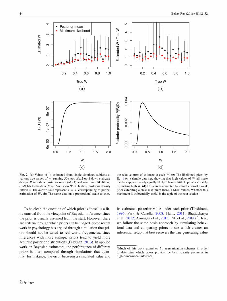
Fig. 2 (a) Values of W estimated from single simulated subjects atvarious true values of W , running 50 steps of a 2-up-1-down staircasedesign. Points show posterior mean (black) and maximum likelihood(red) fits to the data. Error bars show 95 % highest posterior densityintervals. The dotted lines represent y = x, corresponding to perfectestimation of W . (b) The same data on a proportional scale to show

the relative error of estimate at each W . (c) The likelihood given byEq. 1 on a simple data set, showing that high values of W all makethe data approximately equally likely. There is little hope of accuratelyestimating high W . (d) This can be corrected by introduction of a weakprior exhibiting a clear maximum (here, a MAP value). Whether thismaximum is inferentially useful is the topic of the next section

To be clear, the question of which prior is “best” is a lit-tle unusual from the viewpoint of Bayesian inference, sincethe prior is usually assumed from the start. However, thereare criteria through which priors can be judged. Some recentwork in psychology has argued through simulation that pri-ors should not be tuned to real-world frequencies, sinceinferences with more entropic priors tend to yield moreaccurate posterior distributions (Feldman, 2013). In appliedwork on Bayesian estimators, the performance of differentpriors is often compared through simulations that quan-tify, for instance, the error between a simulated value and

its estimated posterior value under each prior (Tibshirani,1996; Park & Casella, 2008; Hans, 2011; Bhattacharyaet al., 2012; Armagan et al., 2013; Pati et al., 2014).3 Here,we follow the same basic approach by simulating behav-ioral data and comparing priors to see which creates aninferential setup that best recovers the true generating value

3Much of this work examines Lp regularization schemes in orderto determine which priors provide the best sparsity pressures inhigh-dimensional inference.

Behav Res (2016) 48:42–52 45

of W , under various assumptions about the best propertiesfor an estimate to have. The primary result is that W canbe better estimated than Eq. 1 by incorporating a prior—inparticular, a 1/W prior—and using a simple MAP (maxi-mum a posteriori) estimate of the posterior mode. As such,this domain provides one place for Bayesian ideas to findsimple, immediate, and nearly effortless, improvements inscientific practice.

The basic problem with W

The essential challenge in estimating W in the psy-chophysics of number is that W plays roughly the same roleas a standard deviation. As such, the range of possible W

is bounded (W ≥ 0) and typical human adults are near the“low” end of this scale, considerably less than 1. A result ofthis is that the reliability of an estimate of W will dependon its value, a situation that violates the assumptions ofessentially all standard statistical analyses (e.g., t tests,ANOVA, regression, correlation, factor analysis, etc.)

Figure 2a illustrates the problem. The x-axis here showsa true value of W which was used to simulate a human’sperformance in a task with 50 responses in a 2-up-1-downstaircased design with n2 always set to n1 + 1. This simula-tion is used for all results in the paper, however the resultspresented are robust to other designs and situations, includ-ing exhaustive testing of numerosities (see Appendix A) andsituations where additional noise factors decrease accuracyat random (see Appendix B). In Fig. 2, a posterior meanestimated W is shown by black dots using a uniform prior,4

and the 95 % highest posterior density region (specifyingthe region where the estimation puts 95 % of its confidencemass) is shown by the black error bars. This range shows theset of values we should consider to be reasonably likely foreach subject, over and above the posterior point estimate inblack. For comparison, a ML fit—using just (1)—is shownin red.

This figure illustrates several key features of estimatingW . First, the error in the estimate depends on the value ofW : higher W s not only have greater likely ranges but alsogreater scatter of the mean (circle) about the line y = x.This increasing variance is seen in both the mean (black)andML fits, and Fig. 2b suggests even the relative error mayincrease as W grows.

Because Bayesian inference represents optimal proba-bilistic inference relative to its assumptions, we may take

4Uniform on [0, 3].

the error bars here as normative, reflecting the certaintywe should have about the value of W given the data. Forinstance, in this figure, the error bars almost all overlap withthe line y = x, which would be a correct estimation of W .From this viewpoint, the increasing error bars show that weshould have more uncertainty about W when it is large thanwhen it is small. The data is simply less informative abouthigh values of W when it is in this range. This is true in spiteof the fact that the same number of data points are gatheredfor each simulated subject.

The reason for this increasing error of estimation isvery simple: Eq. 1 becomes very “flat” for high W dueto the fact that 1/W approaches zero for high values ofW . This is shown in Fig. 2c, giving the value of Eq. 1for various W on a simple data set consisting of ten cor-rect answers on (n1, n2) = (6, 7) and ten incorrect answerson (7, 8). When W is high, it predicts correct answers atthe chance 50 % rate and it matters very little which highvalue of W is chosen (e.g., W = 1.0 vs. W = 2.0), asthe line largely flattens out for high W . As such, choos-ing W to optimize (1) is in the best case error-prone, andthe worst case meaningless for these high values. Figure 2dshows what happens when a prior P(W) ∝ 1/W is intro-duced. Now, we see a clear maximum because althoughthe likelihood is flat, the prior is decreasing, so the poste-rior (shown) has a clear mode. The “optimal” (maximum)value of the line in Fig. 2d might provide a good estimate ofthe true W .

The next two sections address two concerns that Fig. 2ashould raise. First, one might wonder what type of inferen-tial setup would best allow us to estimate W . In this figure,the maximum likelihood estimation certainly looks betterthan posterior mean estimation. The next section consid-ers other types of estimation, different priors on W , anddifferent measures of the effectiveness of an estimate. Thefinal section examines the impact that improved estimationhas on finding correlates W , as well as the consequencesof the fact that our ability to estimate W changes with themagnitude of W itself.

Efficient estimation of W

In general, use of the full Bayesian posterior on W providesa full characterization of our beliefs, and should be usedfor optimal inferences about the relationship between W

and other variables. However, most common statistical toolsdo not handle posterior distributions on variables but ratheronly handle single measurements (e.g., a point estimate ofW ). Here, we will assume that we summarize the posterior

46 Behav Res (2016) 48:42–52

in W with a single point estimate since this is likely the waythe variable will be used in the literature. For each choiceof prior, we consider several different quantitative measuresof how “good” an estimate a point estimate is, using severaldifferent point estimate summaries of the posterior (e.g., themean, median, and mode). The analysis compares each tothe standard ML fitting used by Eq. 1.

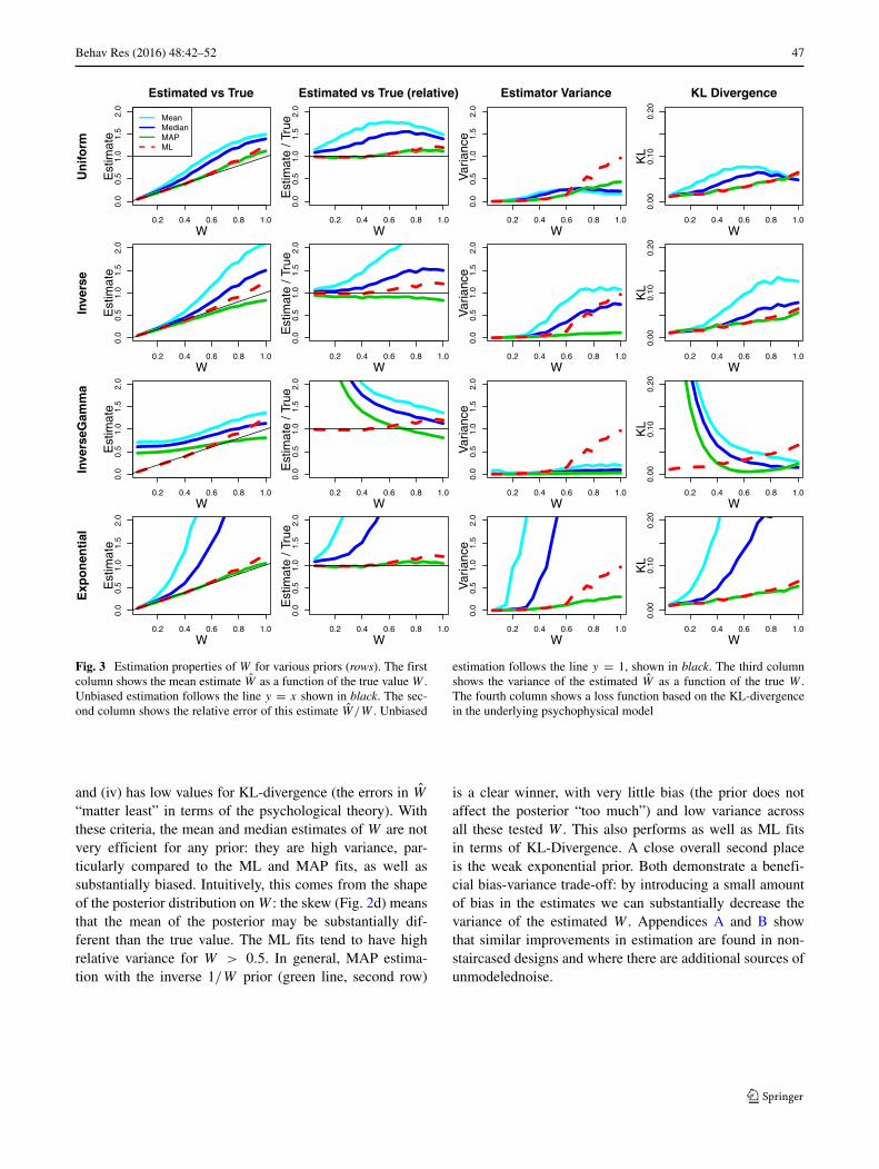
Figure 3 shows estimation of W for several priors andpoint estimate summaries of the posterior, across four dif-ferent measures of an estimate’s quality. Each subplot showsthe true W on the x-axis. The first column shows on themean estimated W for each W , across 1000 simulated sub-jects, using the 2-up-1-down setup used in Fig. 2a. Recoveryof the true W here would correspond to all points lying onthe line y = x. The second column shows the relative esti-mation, W/W at each value of W , providing a measure ofrelative bias. The third column shows the variance in theestimate of W , V ar[W | W ]. Lower values correspondto more efficient estimators of W , meaning that they moreoften have W close to W . The fourth column shows the dif-ference between the estimate and the true value accordingto an information-theoretic loss function. Assuming that aperson’s representation of a number n is Normal(n,Wn),we may capture the effective quality of an estimate W

for the underlying psychological theory by looking at the“distance” between the true distribution Normal(n,Wn)

and the estimated distribution Normal(n, Wn). One natu-ral quantification of the distance between distributions is theKL-divergence (Cover & Thomas, 2006). The fourth columnshows the KL-divergence5 (higher is worse), quantifyingin an information-theoretic sense, how much an estimatedW matters in terms of the psychological model thought tounderlie Weber ratios.

The rows in this figure correspond to four different setsof priors P(W). The first row is a uniform prior P(W) ∝ 1on the intervalW ∈ [0, 3]. Because this prior does not affectthe value of the posterior in this range, it has that P(W |D) = P(D | W), meaning that estimation is essentiallythe same as in ML fitting of Eq. 1. However, unlike (1), theBayesian setup still allows computation of the variability inthe estimated W , as well as posterior means (light blue),and medians (dark blue), in addition to MAPs (green). Forcomparison, each plot also shows the maximum likelihoodfit (1) in red.6

5The KL-divergence goes to infinity as W goes to zero, and some W

are estimated very close to zero. To robustly handle this issue for verylow W , means with 5 % tails trimmed are plotted in the figure.6These are generally identical to MAP, except that the uniform priorrestricts to [0, 3], leading to decreased variance for high W .

The second row shows an inverse prior P(W) ∝1/W . This prior would be the Jeffreys’ prior for esti-mation of a normal standard deviation,7 to which W isclosely related, although the inverse prior is not a Jeffreys’prior for the current likelihood. The inverse prior stronglyprefers low W .

The third row shows another standard prior, an inverse-Gamma prior. This prior is often a convenient one foruse in Bayesian estimation of standard deviations becauseit is conjugate to the normal, meaning that the poste-rior is of the same form as the prior, allowing efficientinference strategies and analytical computation. The showninverse-Gamma uses a shape parameter α = 1 and scaleβ = 1, yielding a peak in the prior at 0.5. The shapeof the inverse-Gamma used here corresponds to somestrong expectations that W is neither too small nor toolarge, but approximately in the right range. Because ofthis, this prior pulls smaller W higher, and higher W

lower, as shown by the second column plot with esti-mates above the line for low W and below the line forhigh W .

The fourth row shows an exponential prior P(W) =λe−λW for λ = 0.1, a value chosen by informal experi-mentation. This corresponds to substantial expectations thatW is small, with pull downwards instead of upwards forsmall W .

From Fig. 3 we are able to read off the most efficientscheme for estimating W under a range of possible consid-erations. For instance, we may seek a prior that gives rise toa posterior with the lowest mean or median KL-Divergence,meaning the row for which the light and dark blue lines,respectively, are lowest in the fourth column. Or, we maycommit to a uniform prior (first row) and ask whetherposterior means, medians, or MAPs provide the best sum-mary of the posterior under each of these measures (likely,MAP). Much more globally, however, we can look acrossthis figure and try to determine which estimation scheme—which prior (column) and posterior summary (line type)—together provide the best overall estimate. In general, weshould seek a scheme that (i) falls along the line (y = x) inthe first column (low bias), (ii) falls along the line y = 1in the second (low relative error), (iii) has the minimumvalue for a range of W in the third column (low variance),

7In that setting, the Jeffreys’ prior is the unique prior that is invariantto transformations (Jaynes, 2003), meaning it does not depend on howwe have formalized (parameterized) (1). In this sense, it “builds in”very little.

Behav Res (2016) 48:42–52 47

0.2 0.4 0.6 0.8 1.0

0.0

0.5

1.0

1.5

2.0

W

Est

imat

e

Un

iform

Estimated vs True

MeanMedianMAPML

0.2 0.4 0.6 0.8 1.0

0.0

0.5

1.0

1.5

2.0

W

Est

imat

e / T

rue

Estimated vs True (relative)

0.2 0.4 0.6 0.8 1.0

0.0

0.5

1.0

1.5

2.0

W

Var

ianc

e

Estimator Variance

0.2 0.4 0.6 0.8 1.0

0.00

0.10

0.20

W

KL

KL Divergence

0.2 0.4 0.6 0.8 1.0

0.0

0.5

1.0

1.5

2.0

W

Est

imat

e

Inve

rse

0.2 0.4 0.6 0.8 1.0

0.0

0.5

1.0

1.5

2.0

W

Est

imat

e / T

rue

0.2 0.4 0.6 0.8 1.0

0.0

0.5

1.0

1.5

2.0

W

Var

ianc

e

0.2 0.4 0.6 0.8 1.0

0.00

0.10

0.20

W

KL

0.2 0.4 0.6 0.8 1.0

0.0

0.5

1.0

1.5

2.0

W

Est

imat

e

Inve

rseG

amm

a

0.2 0.4 0.6 0.8 1.0

0.0

0.5

1.0

1.5

2.0

W

Est

imat

e / T

rue

0.2 0.4 0.6 0.8 1.0

0.0

0.5

1.0

1.5

2.0

W

Var

ianc

e

0.2 0.4 0.6 0.8 1.0

0.00

0.10

0.20

W

KL

0.2 0.4 0.6 0.8 1.0

0.0

0.5

1.0

1.5

2.0

W

Est

imat

e

Exp

on

enti

al

0.2 0.4 0.6 0.8 1.0

0.0

0.5

1.0

1.5

2.0

W

Est

imat

e / T

rue

0.2 0.4 0.6 0.8 1.0

0.0

0.5

1.0

1.5

2.0

W

Var

ianc

e

0.2 0.4 0.6 0.8 1.0

0.00

0.10

0.20

WK

L

Fig. 3 Estimation properties of W for various priors (rows). The firstcolumn shows the mean estimate W as a function of the true value W .Unbiased estimation follows the line y = x shown in black. The sec-ond column shows the relative error of this estimate W/W . Unbiased

estimation follows the line y = 1, shown in black. The third columnshows the variance of the estimated W as a function of the true W .The fourth column shows a loss function based on the KL-divergencein the underlying psychophysical model

and (iv) has low values for KL-divergence (the errors in W

“matter least” in terms of the psychological theory). Withthese criteria, the mean and median estimates of W are notvery efficient for any prior: they are high variance, par-ticularly compared to the ML and MAP fits, as well assubstantially biased. Intuitively, this comes from the shapeof the posterior distribution on W : the skew (Fig. 2d) meansthat the mean of the posterior may be substantially dif-ferent than the true value. The ML fits tend to have highrelative variance for W > 0.5. In general, MAP estima-tion with the inverse 1/W prior (green line, second row)

is a clear winner, with very little bias (the prior does notaffect the posterior “too much”) and low variance acrossall these tested W . This also performs as well as ML fitsin terms of KL-Divergence. A close overall second placeis the weak exponential prior. Both demonstrate a benefi-cial bias-variance trade-off: by introducing a small amountof bias in the estimates we can substantially decrease thevariance of the estimated W . Appendices A and B showthat similar improvements in estimation are found in non-staircased designs and where there are additional sources ofunmodelednoise.

48 Behav Res (2016) 48:42–52

The success of the MAP estimator over the mean mayhave more general consequences for Bayesian data analysisin situations like these where the likelihood is relatively flat(e.g., Fig. 2c). Here, the flatness of the likelihood leads tostill a broad posterior (Fig. 2d). This is what leads posteriormean estimates of W to be much less useful than posteriorMAP estimates.

It is important to point out that the present analysishas assumed each subject’s W is estimated independentlyfrom any others. This assumption is a simplification thataccords with standard ML fitting. Even better estimationcould likely be developed using a hierarchical model inwhich the group distribution of W is estimated for a num-ber of subjects, and those subject estimates are informed bythe group distribution. This approach, for instance, leads tomuch more powerful and sensible results in the domain ofmixed-effect regression (Gelman & Hill, 2007). It is beyondthe scope of the current paper to develop such a model, buthierarchical approaches will likely prove beneficial in manydomains, particularly where distinct group mean W s mustbe compared.

Power and heteroskedasticity in estimating W

We next show that improved estimates of W lead toimproved power in looking for correlates of W , a fact thatmay have consequences for studies that examine factorsthat do and—especially—do not correlate with approximatenumber acuity. A closely related issue to statistical power isthe impact of the inherent variability in our estimation ofW .In different situations, ignoring the property that higher W

are estimated higher noise can lead to either reduced power(type I errors) or anticonservativity (type II errors) (Hayes& Cai, 2007).

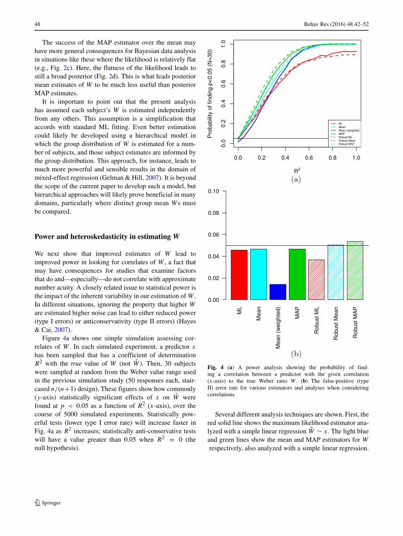
Figure 4a shows one simple simulation assessing cor-relates of W . In each simulated experiment, a predictor x

has been sampled that has a coefficient of determinationR2 with the true value of W (not W ). Then, 30 subjectswere sampled at random from the Weber value range usedin the previous simulation study (50 responses each, stair-cased n/(n+1) design). These figures show how commonly(y-axis) statistically significant effects of x on W werefound at p < 0.05 as a function of R2 (x-axis), over thecourse of 5000 simulated experiments. Statistically pow-erful tests (lower type I error rate) will increase faster inFig. 4a as R2 increases; statistically anti-conservative testswill have a value greater than 0.05 when R2 = 0 (thenull hypothesis).

Fig. 4 (a) A power analysis showing the probability of find-ing a correlation between a predictor with the given correlation(x-axis) to the true Weber ratio W . (b) The false-positive (typeII) error rate for various estimators and analyses when consideringcorrelations

Several different analysis techniques are shown. First, thered solid line shows the maximum likelihood estimator ana-lyzed with a simple linear regression W ∼ x. The light blueand green lines show the mean and MAP estimators for W

respectively, also analyzed with a simple linear regression.

Behav Res (2016) 48:42–52 49

The dark blue line corresponds to a weighted regressionwhere the points have been weighted by their reliability.8

The dotted lines correspond to use of heteroskedasticity-consistent estimators, via the sandwich package in R(Zeileis, 2004). This technique, developed in the economet-ric literature, allows computation of standard errors and p

values in a way that is robust to violations of homoscedas-ticity.

This figure makes it clear first that the ML estimatortypically used is underpowered relative to mean or MAPestimators. This is most apparent for R2s above 0.3 orso, for which the MAP estimators have a much higherprobability of detecting an effect than the ML estimators.This has important consequences for null results, or com-parisons between groups where one shows a significantdifference in W and another does not, particularly whensuch comparison are (incorrectly) not analyzed as inter-actions (Nieuwenhuis et al., 2011). The increased powerfor non-ML estimations seen in Fig. 4a indicates thatsuch estimators should be strongly preferred by researchersand reviewers.

The value for R2 = 0 (left end of the plot) corre-sponds to the null hypothesis of no relationship. For clarity,the value of the lines have been replotted in Fig 4b. Barsabove the line 0.05 would reflect statistical anticonserva-tivity, where the method has a greater than 5 % chance offinding an effect when the null (R2 = 0) is true. This figureshows that these methods essentially do not increase thetype-II error rates with a possible very minor anticonserva-tivity for robust regressions with the MAP estimate.9 Useof the weighted regression is particularly conservative. Ingeneral, the heteroskedasticity found in estimating W is notlikely to cause problems when un-modeled in this simplecorrelational analysis.

8 There is some subtlety in correctly determining these weights. Forthis plot, the posterior variance was determined through MCMC sam-pling. The optimal weighting in a regression (i.e., the weighting whichleads to the unbiased, minimal variance estimator) weights points pro-portional to the inverse variance at each point. However, in R, thisvariance must include the residual variance, not solely the measure-ment error on W . Therefore, the regression was run in two stages: first,a model was run using the inverse variance as weights in R. Then, theresidual error was computed and added back into the estimation erroron W .9Error bars are not shown in this graph since they are very small as aresult of the number of simulated studies run.

Conclusions

This paper has examined estimation of W in the contextof a number of common considerations. Simulations herehave shown that MAP estimation with a 1/W prior allowsefficient estimation across a range of W (Fig. 3) and con-sidering a variety of important features of good estimation.This scheme introduces a small bias on W that helps to cor-rect the large uncertainty about W that occurs for highervalues. Its use leads to statistical tests that are more pow-erful than the standard maximum likelihood fits given byEq. 1. When used in simple correlational analyses, many ofthe standard analysis techniques do not introduce increasedtype-II error rates, despite the heteroskedasticity inherent inestimating W .

Instructions for estimation The recommended 1/W prioris extremely easy to use, including only a − logW termin addition to the log likelihood that is typically fit. Ifsubjects were shown pairs of numbers (ai, bi) and ri isa binary variable indicating whether they responded cor-rectly (ri = 1) or incorrectly (ri = 0), we can fit W tomaximize

− logW +∑

i

log

⎛⎜⎝ri · �

⎡⎢⎣ |ai − bi |

W ·√

a2i + b2i

⎤⎥⎦

+(1 − ri) ·⎛⎜⎝1 − �

⎡⎢⎣ |ai − bi |

W ·√

a2i + b2i

⎤⎥⎦

⎞⎟⎠

⎞⎟⎠ . (2)

In R (Core Team, 2013), we can estimate W via

where ai, bi and ri are vectors of ai , bi , and ri , respec-tively. Note that the use of MAP estimation here (ratherthan ML) amounts to simply inclusion of the −log(W)

term in each. The ease and clear advantages of thismethod should lead to its adoption in research on theapproximate number system and related psychophysicaldomains.

50 Behav Res (2016) 48:42–52

Appendix A: Estimation in a non-staircased design

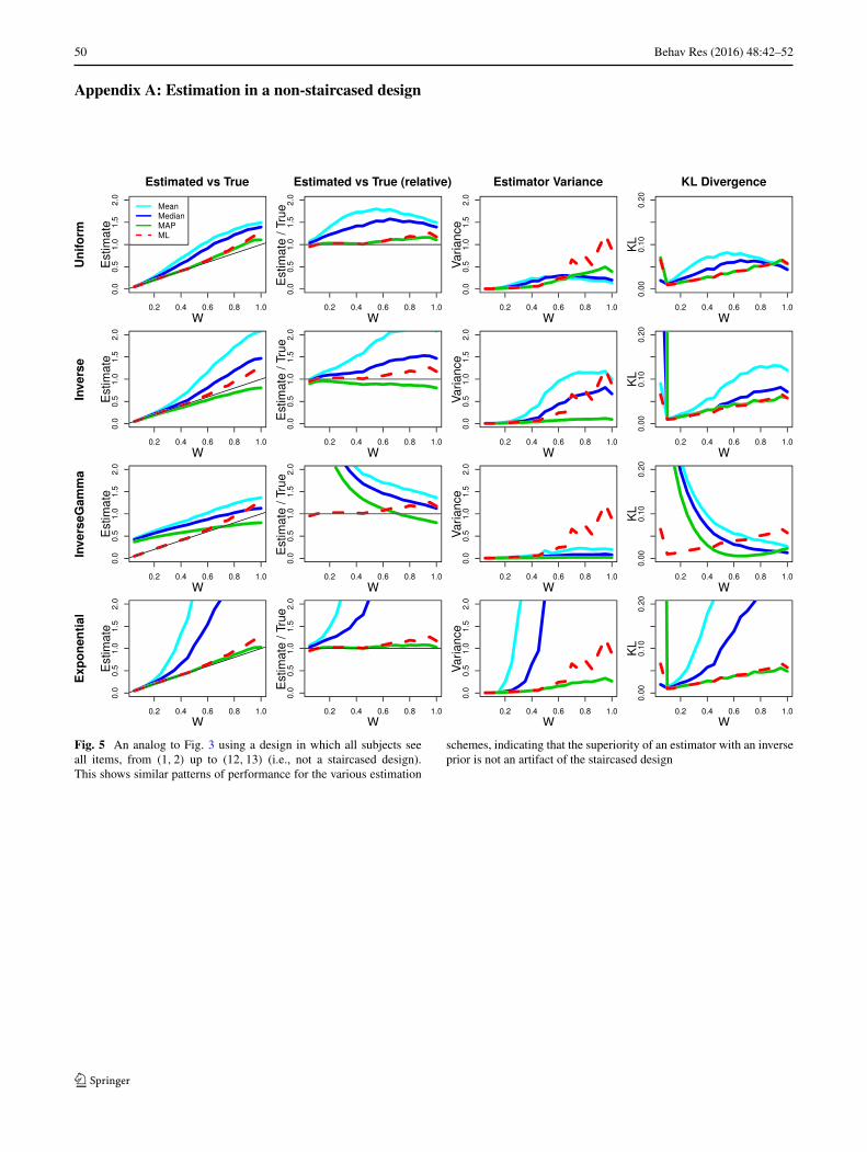
Fig. 5 An analog to Fig. 3 using a design in which all subjects seeall items, from (1, 2) up to (12, 13) (i.e., not a staircased design).This shows similar patterns of performance for the various estimation

schemes, indicating that the superiority of an estimator with an inverseprior is not an artifact of the staircased design

Behav Res (2016) 48:42–52 51

Appendix B: Estimation with unmodeled noise

Fig. 6 An analog to Fig. 3 in the situation where subjects make mis-takes 10 % of the time, independent of the displayed stimuli (forinstance, through inattention). This demonstrates that the efficientperformance of the inverse prior holds even when the fit model is

somewhat misspecified in that it neglects the extra noise. Note that inthis case, the estimators tend to over-estimate W since the additionalnoise leads them to conclude that W is worse (higher) than it truly is.Note that the ML fit performs particularly poorly in this situation

52 Behav Res (2016) 48:42–52

References

Armagan, A., Dunson, D.B., & Lee, J. (2013). Generalized doublePareto shrinkage. Statistica Sinica, 23(1), 119.

Bhattacharya, A., Pati, D., Pillai, N.S., & Dunson, D.B. (2012).Bayesian shrinkage. arXiv:1212.6088

Bonny, J.W., & Lourenco, S.F. (2013). The approximate number sys-tem and its relation to early math achievement: evidence fromthe preschool years. Journal of Experimental Child Psychology,114(3), 375–388.

Cover, T., & Thomas, J. (2006). Elements of information theory.Hoboken: Wiley.

Dehaene, S. (1997). The number sense: how the mind creates mathe-matics. USA: Oxford University Press.

Dehaene, S., Izard, V., Spelke, E., & Pica, P. (2008). Log or linear?Distinct intuitions of the number scale in Western and Amazonianindigene cultures. Science, 320(5880), 1217–1220.

Fechner, G. (1860). Elemente der psychophysik. Leipzig: Breitkopf &Hartel.

Feldman, J. (2013). Tuning your priors to the world. Topics in Cogni-tive Science, 5(1), 13–34.

Frank, M.C., Fedorenko, E., & Gibson, E. (2008). Language as a cog-nitive technology: English speakers match like Pirah when youdon’t let them count. In Proceedings of the 30th annual meeting ofthe Cognitive Science Society.

Gallistel, C., & Gelman, R. (1992). Preverbal and verbal counting andcomputation. Cognition, 44, 43–74.

Gelman, A., & Hill, J. (2007). Data analysis using regression andmultilevel/hierarchical models. Cambridge: Cambridge UniversityPress.

Gibbon, J. (1977). Scalar expectancy theory andWeber’s law in animaltiming. Psychological Review, 84(3), 279.

Gilmore, C., Attridge, N., & Inglis, M. (2011). Measuring the approx-imate number system. The Quarterly Journal of ExperimentalPsychology, 64(11), 2099–2109.

Halberda, J., & Feigenson, L. (2008). Developmental change in theacuity of the “number sense”: the approximate number system in3-, 4-, 5-, and 6-year-olds and adults. Developmental Psychology,44(5), 1457.

Halberda, J., Ly, R., Wilmer, J., Naiman, D., & Germine, L. (2012).Number sense across the lifespan as revealed by a massiveinternet-based sample. Proceedings of the National Academy ofSciences, 109(28), 11116–11120.

Halberda, J., Mazzocco, M., & Feigenson, L. (2008). Individualdifferences in non-verbal number acuity correlate with mathsachievement. Nature, 455(7213), 665–668.

Hans, C. (2011). Elastic net regression modeling with the orthantnormal prior. Journal of the American Statistical Association,106(496), 1383–1393.

Hayes, A.F., & Cai, L. (2007). Using heteroskedasticity-consistentstandard error estimators in OLS regression: an introductionand software implementation. Behavior Research Methods, 39(4),709–722.

Jaynes, E. (2003). Probability theory: The logic of science: CambridgeUniversity Press.

Kruschke, J. (2010a). Bayesian data analysis. Wiley InterdisciplinaryReviews: Cognitive Science, 1(5), 658–676.

Kruschke, J. (2010b). Doing Bayesian data analysis: a tutorial with Rand BUGS. Brain, 1(5), 658–676.

Kruschke, J. (2010c). What to believe: Bayesian methods for dataanalysis. Trends in Cognitive Sciences, 14(7), 293–300.

Lee, M., & Sarnecka, B. (2010). A model of knower-level behavior innumber concept development. Cognitive Science, 34(1), 51–67.

Lee, M., & Sarnecka, B.W. (2011). Number-knower levels in youngchildren: insights from Bayesian modeling. Cognition, 120(3),391–402.

Masin, S., Zudini, V., & Antonelli, M. (2009). Early alternative deriva-tions of Fechner’s law. Journal of the History of the BehavioralSciences, 45(1), 56–65.

Meck, W.H., & Church, R.M. (1983). A mode control model of count-ing and timing processes. Journal of Experimental Psychology:Animal Behavior Processes, 9(3), 320.

Mussolin, C., Nys, J., & Leybaert, J. (2012). Relationships betweenapproximate number system acuity and early symbolic numberabilities. Trends in Neuroscience and Education, 1(1), 21–31.

Nieder, A., & Dehaene, S. (2009). Representation of number in thebrain. Annual Review of Neuroscience, 32, 185–208.

Nieder, A., Freedman, D., & Miller, E. (2002). Representation of thequantity of visual items in the primate prefrontal cortex. Science,297(5587), 1708–1711.

Nieder, A., & Merten, K. (2007). A labeled-line code for small andlarge numerosities in the monkey prefrontal cortex. Journal ofNeuroscience, 27(22), 5986–5993.

Nieder, A., & Miller, E. (2004). Analog numerical representationsin rhesus monkeys: evidence for parallel processing. Journal ofCognitive Neuroscience, 16(5), 889–901.

Nieuwenhuis, S., Forstmann, B.U., & Wagenmakers, E.-J.(2011). Erroneous analyses of interactions in neuroscience:A problem of significance. Nature Neuroscience, 14(9), 1105–1107.

Park, T., & Casella, G. (2008). The Bayesian lasso. Journal of theAmerican Statistical Association, 103(482), 681–686.

Pati, D., Bhattacharya, A., Pillai, N. . S., Dunson, D., & et al.(2014). Posterior contraction in sparse Bayesian factor modelsfor massive covariance matrices. The Annals of Statistics, 42(3), 1102–1130.

Pica, P., Lemer, C., Izard, V., & Dehaene, S. (2004). Exact andapproximate arithmetic in an Amazonian indigene group. Science,306(5695), 499.

Portugal, R., & Svaiter, B. (2011). Weber–Fechner law and the opti-mality of the logarithmic scale. Minds and Machines, 21(1), 73–81.

Core Team, R. (2013). R: A language and environment for statisticalcomputing [Manuel de logiciel]. Vienna.

Sun, J., Wang, G., Goyal, V., & Varshney, L. (2012). A frame-work for Bayesian optimality of psychophysical laws. Journal ofMathematical Psychology.

Tibshirani, R. (1996). Regression shrinkage and selection via the lasso.Journal of the Royal Statistical Society, 267–288.

Whalen, J., Gallistel, C., & Gelman, R. (1999). Nonverbal counting inhumans: the psychophysics of number representation. Psycholog-ical Science, 10(2), 130–137.

Zeileis, A. (2004). Econometric computing with HC and HAC covari-ance matrix estimators.