Efficient Operation of Natural Gas Transmission Systems: A Network

Efficient Operation of Natural Gas Transmission Systems:

A Network-Based Heuristic for Cyclic Structures

Roger Z. Rıos-Mercado1

Graduate Program in Systems Engineering

Universidad Autonoma de Nuevo León

AP 111 – F, Cd. Universitaria

San Nicolas de los Garza, NL 66450, México

E-mail: [email protected]

Seongbae Kim

Institute of Information Technology, Inc.

2203 Timberloch Place, Suite 100

The Woodlands, TX 77380, USA


E. Andrew Boyd

PROS Revenue Management

3100 Main Street, Suite 900

Houston, TX 77002, USA


July 2003

1Corresponding author

Abstract

Gas transmission network problems differ from traditional network flow problems in some funda-

mental aspects. First, in addition to the flow variables for each arc, which in this case represent mass

flow rates, a pressure variable is defined at every node. Second, besides the mass balance constraints,

there exist two other types of constraints: (i) a nonlinear equality constraint on each pipe, which rep-

resents the relationship between the pressure drop and the flow; and (ii) a nonlinear non-convex set

which represents the feasible operating limits for pressure and flow within each compressor station. The

objective function is given by a nonlinear function of flow rates and pressures. In the real world, these

type of instances are very large both in terms of the number of decision variables and the number of

constraints, and very complex due to the presence of non-linearity and non-convexity in both the set of

feasible solutions and the objective function.

In this paper we propose a heuristic solution procedure for fuel cost minimization on gas transmis-

sion systems with a cyclic network topology, that is, networks with at least one cycle containing two

or more compressor station arcs. Our heuristic solution methodology is based on a two-stage iterative

procedure. In a particular iteration, at a first stage, gas flow variables are fixed and optimal pressure

variables are found via dynamic programming. At a second stage, pressure variables are fixed and an

attempt is made to find a set of flow variables that improve the objective function by exploiting the

underlying network structure. Empirical evidence supports the effectiviness of the proposed procedure.

Keywords: natural gas, pipeline optimization, transmission networks, heuristic, dynamic programming

1 Introduction

As natural gas pipeline systems have grown larger and more complex, the importance of optimum

operation and planning of these facilities has increased. The investment costs and operation expenses of

pipeline networks are so large that even small improvements in system utilization can involve substantial

amounts of money.

The natural gas industry services include producing, moving, and selling gas. Our main interest in

this study is focused on the transportation of gas through a pipeline network. Moving gas is divided

into two classes: transmission and distribution. Transmission of gas means moving a large volume of

gas at high pressures over long distances from a gas source to distribution centers. In contrast, gas

distribution is the process of routing gas to individual customers. For both transmission and distribution

networks, the gas flows through various devices including pipes, regulators, valves, and compressors.

In a transmission network, gas pressure is reduced due to friction with the pipe wall as the gas travels

through the pipe. Some of this pressure is added back at compressor stations, which raises the pressure

of the gas passing through them.

In a gas transmission network, the overall operating cost of the system is highly dependent upon the

operating cost of the compressor stations in a network. A compressor station’s operating cost, however,

is generally measured by the fuel consumed at the compressor station. According to Luongo, Gilmour,

and Schroeder [12], the operating cost of running the compressor stations represents between 25% and

50% of the total company’s operating budget. Hence, the objective for a transmission network is to

minimize the total fuel consumption of the compressor stations while satisfying specified delivery flow

rates and minimum pressure requirements at the delivery terminals.

Depending on how the gas flow changes with respect to time, we distinguish between systems in

steady state and transient state. A system is said to be in steady state when the values characterizing the

flow of gas in the system are independent of time. In this case, the system constraints, particularly the

ones describing the gas flow through the pipes, can be described using algebraic non-linear equations.

In contrast, transient analysis requires the use of partial differential equations to describe such relation-

ships. This makes the problem considerably harder to solve from the optimization perspective. In fact,

optimization of transient models is one of the most challenging areas of opportunity for future research.

In the case of transient optimization, variables of the system, such as pressures and flows, are functions

of time. In this work, we focus on steady-state gas transmission network problems with the objective of

minimizing the operational costs.

Gas transmission network problems differ from traditional network flow problems in some funda-

mental aspects. First, in addition to the flow variables for each arc, which in this case represent mass

flow rates, a pressure variable is defined at every node. Second, besides the mass balance constraints,

there exist two other types of constraints: (i) a nonlinear equality constraint on each pipe, which rep-

resents the relationship between the pressure drop and the flow; and (ii) a nonlinear non-convex set

1

which represents the feasible operating limits for pressure and flow within each compressor station. The

objective function is given by a nonlinear function of flow rates and pressures.

The problem is very difficult due to the presence of a non-convex objective function and non-convex

feasible region. Optimization algorithms (most of them based on dynamic programming) for non-cyclic

gas network topologies are in a relatively well developed stage. However, effective algorithms for cyclic

topologies are practically non-existent. So our work focuses on addressing gas transmission problems

on cyclic topologies. A cyclic topology is a network with at least one cycle containing two or more

compressor station arcs.

In this paper we propose a heuristic solution procedure for fuel cost minimization on gas trans-

mission systems with a cyclic network topology. Our heuristic solution methodology is based on a

two-stage iterative procedure. In a particular iteration, at a first stage, gas flow variables are fixed and

optimal pressure variables are found via dynamic programming. At a second stage, the pressure vari-

ables are fixed and an attempt is made to find a set of flow variables that improve the objective function

by exploiting the underlying network structure. Empirical evidence supports the effectiviness of this

proposed procedure.

The organization of this paper is as follows. In Section 2 we introduce the gas transmission network

problem and present the mathematical model. Section 3 presents a survey of previous related work. In

Section 4, we present the network formulation of the gas transmission system and discuss the network

decomposition. In Section 5, we describe the proposed algorithm. Implementation, numerical examples

and computational experiments are reported in Section 6. This is followed by our conclusions and

directions for future research in Section 7.

2 Problem Definition

A gas transmission network is composed of pipelines, junction nodes, including supply and delivery

nodes, and compressor stations. The existence of compressor stations in the network is one of the key

characteristics of a gas transmission network. The transmission segment operates systems of pipes and

compressors and attempts to move large quantities of gas over long distances. When traveling through

the pipes, the gas pressure is reduced by friction with the pipe walls. Some of this pressure is added

back at the compressor stations.

Compressor stations in a transmission network are complex entities typically involving a number

of compressor units arranged in parallel or in serial at one location. The operating cost of the gas

transmission network is usually ruled by the operating cost of the compressor stations. Therefore,

representing compressor stations within a network configuration is quite an important issue and the way

of representing them varies according to the solution methodology. We now present the model we use

for this problem and discuss the most important assumptions.

2

2.1 Model for Steady-State Problem

Let � � �� be a directed network defined by a set� of � nodes, a set� of � pipes, and

a set� of � compressor stations. Note that the set of arcs� in � is defined as� � � ��, with

�� . The decision variables are�� , the mass flow rate at arc�� and�, the gas pressure

at node� � � . At each node� � � , there is a known parameter� called the net flow through that

node. Clearly,� � � (� � �) implies node� is a source (delivery) node, whereas� � � means node

� is just a transhipment node. In addition, pressure limits�� and�� are given at every node. For each

pipe�� the pipe resistance ��, which is computed from the pipe physical properties, is assumed to be

known.

Note also that for each arc�� there are three associated variables:�� , � and �. In

particular, in a compressor station arc,� and� are called suction and discharge pressures, respectively.

The goal of the problem is to minimize the total fuel consumption used by the stations while satis-

fying specified delivery requirements throughout the system. We assume that there is no transportation

cost associated with ordinary pipes. The cost function is only defined at each compressor station, which

is given by a function�� described below.

The mathematical formulation of the gas transmission network problem (GTN) is given by

(GTN) minimize�

��

�� (1a)

subject to�

��

��

��

�� (1b)

��

�� (1c)

� � �� (1d)

�� (1e)

where�� is the feasible operating domain of compressor station�� and�� is the fuel

consumed at station�� .

Flow balance conservation is given by Equation (1b). Constraint (1c) represents the dynamics of

the pipe flow under isothermal and steady-state assumptions. The compressor station constraints (1e)

are not expressed explicitly here. It suffices to know that the feasible set�� is a non-convex set. The

details can be found in Wu et al. [28].

For measuring fuel consumption, we use a function� which is given by

��

��

��

�

��

��

where the adiabatic efficiency�� is assumed constant and is fixed at its maximum value. A more detailed

study on the nature of both the compressor station domain and the fuel consumption function is given

in [28].

3

The problem is very difficult due to the non-convex nature of both the objective function and the

feasible region. Furthermore, the feasible domain�� of the compressor station is not represented in

algebraic form, but as a result of curve fitting methods based on empirical data for the compressor units

used. Also, the type of underlying network topology becomes a crucial issue. That is, depending on the

underlying network configuration, the problem can be more difficult to solve. We will discuss this issue

in more detail in Section 4.

3 Literature Review

Dynamic programming (DP) has been by far the most popular technique for solving many classes of

natural gas pipeline networks since the late 1960s. One of the main reasons is that, in a DP framework,

it is relatively easy to satisfy the pipeline constraints and to handle the non-convexity of the feasible

domain. Other techniques such as mathematical programming and hierarchical control methods have

been applied as well with modest degrees of success. Mathematical programming is usually used for

cyclic systems. Hierarchical control techniques can be more effective when the model of the compressor

station is fairly complicated. In the following sections we present an overview of the most relevant work

done on the solution methodologies used for steady state gas transmission networks.

3.1 Mathematical Programming Approaches

As we have seen in Section 2, problem GTN has a non-convex feasible region, and a non-convex

objective function. In fact, it has been reported by Wu et al. [28] that this objective function typically

has many local optima. These problem features make it very difficult to solve using classical techniques

from mathematical programming. Several researchers have tried to apply mathematical programming

techniques, but their approaches are based on inaccurate or oversimplified models of the compressor

stations. Next we review the most significant works related with mathematical programming, which has

been rather limited.

Pratt and Wilson [19] propose a successive mixed integer linear programming method. Their al-

gorithm solves the nonlinear optimization problem iteratively by linearizing the pressure drop-flow

equations (1c). Integer variables are included in the formulation for compressor unit selection, and

the problem is solved using branch and bound. Percell and Ryan [18] propose an algorithm using a gen-

eralized reduced gradient method for minimizing the fuel consumption problem for a gas transmission

network. We reemphasize the difficulties in handling the nonlinear equality constraints and the complex

nature of the compressor stations in the gas transmission network as the key factors in the relatively

poor success of mathematical programming approaches.

4

3.2 Hierarchical Control Approaches

Difficulty in solving a gas transmission network problem in an integrated way calls for other tech-

niques, such as hierarchical structure in the solution process, which in turn demands an efficient method

for decomposing of the problem. In a hierarchical control approach (Singh [22]), the overall network

is decomposed into two levels: (i) the network state level and (ii) the compressor station level. The

compressor station problem is the lowest level and the network state problem is the highest level. The

local optimization of the compressor stations at the lowest level is the firm basis for an optimization

procedure for the global minimization of total cost. Optimization of the compressor station subproblem

has been studied previously by Osiadacz [13], Percell and Van Reet [17], and Wu, Boyd, and Scott [27].

Larson and Wismer [11] propose a hierarchical control approach for a transient operation of a gun-

barrel pipeline system. Osiadacz and Bell [15] suggest a simplified algorithm for the optimization of

the transient gas transmission network, which is based on a hierarchical control approach. The hierar-

chical control approach for transient models can be found in Anglard and David [2], Osiadacz [14], and

Osiadacz and Swierczewski [16]. Some degree of success has been reported from these approaches as

far as optimizing the compressor station subproblem. However, these approaches have limitations in

globally optimizing the minimum cost. As mentioned in Carter, Schroeder, and Harbick [6], numerical

simulation of the behavior of the gas transmission network is quite widespread, and with a successful

compressor station optimizer, these simulations are quite accurate. However, little work has been done

or even attempted in optimizing the gas transmission network. After the introduction of the hierarchical

control approach, in which detailed compressor station optimization is attached as a lower level sub-

problem, several approaches have focused on the optimization of the higher level problem, the network

state problem.

3.3 Dynamic Programming Approaches

Dynamic programming (DP) (Dreyfus and Law [8]) was first used for a steady state gas transmission

system in Wong and Larson [24, 25]. The authors apply DP to the gunbarrel and diverging branch tree

systems to solve the network state problem. The gunbarrel system, which is basically a single-path

topology, posseses an appropriate serial structure so it can be solved via DP. For the diverging branch

problem, the overall problem is decomposed into a sequence of several one-dimensional DP problems,

each of which deals with a single branch.

There are, however, some limitations to the DP method described by Wong and Larson. First, its

application is limited only to tree networks. Second, the method assumes that there is only a single

compressor unit installed within each compressor station. In addition, the feasible domain of the com-

pressor station is oversimplified in order to make an easier solution process. A successful commercial

optimizer for tree-structured gas transmission networks using DP was developed by Zimmer [29], and

Lall and Percell [10].

5

When applying DP, the underlying network configuration of the given problem can enhance the

solution process. Note that for these non-cyclic systems, the DP formulation is one-dimensional and

can be easily applied because it has been shown [21] that the flow variables can be uniquely determined

beforehand and thus eliminated from the problem, so we only deal with the pressure variables. That

is, in a tree network, once both supply and delivery flow rates are given, the steady state flows can be

uniquely determined. This nice property does not hold for a cyclic system. The existence of cycles

breaks the serial structure, so the flow variables must be explicitly handled, which makes the underlying

DP multidimensional.

The DP approach for cyclic systems has been limited. There were some efforts in applying DP on

the nonsequential structure for applications in chemical engineering problems. Two of the earliest works

include Wilde [23] and Aris, Nemhauser, and Wilde [3]. Both groups treated cycles via “cuts”, i.e., they

cut one end of a cycle in the system and treat the resulting system using DP for tree structures. More

general issues of the nonsequential DP can be found in Bertele and Brioschi [4].

Although several researchers over the years have addressed branched systems in the gas transmission

problem, cyclic systems were not addressed until Luongo, Gilmour, and Schroeder [12]. In their study,

the authors apply DP with the assumption that the flow rates through pipes and at the compressor stations

are fixed. After solving the DP problem with prefixed flow rates, they use a direct search method with

multiple restarts on different flow settings. Thus their approach is a hybrid of DP and either brute-force

enumeration or simulated annealing, depending on problem size. Recently Carter [5] proposed a DP

approach on more general structures with flow rates being fixed. A more detailed description of DP

approaches to gas transmission networks can be found in R´ıos-Mercado [20].

The principal obstacle to date using DP is that its application is limited in practice to simple struc-

tures. Otherwise, the computational effort becomes too large to be practical. This leads to an interesting

question of how to find the optimal setting of the flow variables and how to modify the current flow

setting to obtain a better objective value. This study focuses on these issues.

4 Natural Gas Network Decomposition

In our solution procedure, we first decompose the original graph into several subgraphs (not con-

taining compressor stations), and we further contract each subgraph, yielding a reduced network. It

turns out that the network configuration for each subgraph is not crucial, while the network configura-

tion of the reduced network is critical. In this section we will see how the underlying network topology

becomes a key issue, and plays a very important role in developing solution procedures for this problem.

6

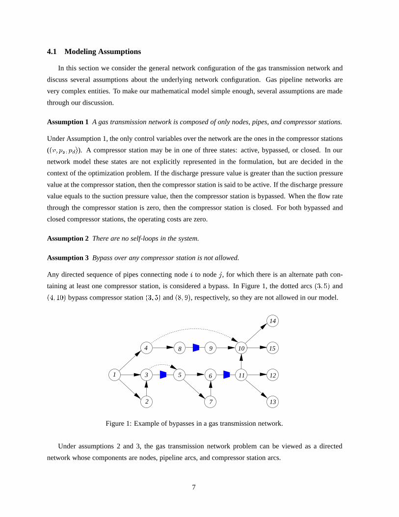
4.1 Modeling Assumptions

In this section we consider the general network configuration of the gas transmission network and

discuss several assumptions about the underlying network configuration. Gas pipeline networks are

very complex entities. To make our mathematical model simple enough, several assumptions are made

through our discussion.

Assumption 1 A gas transmission network is composed of only nodes, pipes, and compressor stations.

Under Assumption 1, the only control variables over the network are the ones in the compressor stations

(�� ). A compressor station may be in one of three states: active, bypassed, or closed. In our

network model these states are not explicitly represented in the formulation, but are decided in the

context of the optimization problem. If the discharge pressure value is greater than the suction pressure

value at the compressor station, then the compressor station is said to be active. If the discharge pressure

value equals to the suction pressure value, then the compressor station is bypassed. When the flow rate

through the compressor station is zero, then the compressor station is closed. For both bypassed and

closed compressor stations, the operating costs are zero.

Assumption 2 There are no self-loops in the system.

Assumption 3 Bypass over any compressor station is not allowed.

Any directed sequence of pipes connecting node� to node�, for which there is an alternate path con-

taining at least one compressor station, is considered a bypass. In Figure 1, the dotted arcs�� and

�� bypass compressor station�� and�� , respectively, so they are not allowed in our model.

1

4

3

2

5 6

7

8 9 10

11 12

13

14

15

Figure 1: Example of bypasses in a gas transmission network.

Under assumptions 2 and 3, the gas transmission network problem can be viewed as a directed

network whose components are nodes, pipeline arcs, and compressor station arcs.

7

Assumption 4 At each node � � � of �, the net inflow � is assumed to be known with certainty.

Moreover, at each delivery node, minimum requirement of the pressure is assumed to be known.

Assumption 5 A gas transmission network can have multiple source nodes from which gas enters the

system. We assume, however, that there is only one source node (super source), which regulates the

input pressure value of the whole system.

By assumption 5, we have only one reference pressure with which our solution procedure works.

The purpose and the effect of these assumptions will be explained in detail in a later section. There are

other assumptions on the configuration of the gas transmission network, and they will be discussed in

the relevant sections.

4.2 Decomposition

Now consider the gas transmission network� � �� , with � nodes,� pipes, and� compres-

sor stations, and its mathematical model GTN defined in (1). Let�� be the�� node-pipe incidence

matrix,�� be the�� node-compressor station incidence matrix, and� � �� . The equality

constraint set of the problem GTN can be represented in a vector form by��

��

(2)

where��

and�� is the vector of�� , in which�� .

Since we assume that there is no bypass, if we delete every compressor station from the entire

system, then we have disconnected subgraphs, each one of which being composed only of pipes and

nodes. Figure 2 shows an example of the subgraphs created by deleting compressor stations.

Each node or pipe of the� belongs to exactly one subgraph. It follows that the subgraphs of�

determine a unique partition of its nodes and pipes. Assume that there are� subgraphs. Let��

�� , be the subgraph defined by a set of nodes,��, and a set of pipes,��. We assume

�� has�� nodes and�� pipes. Note that the nodes in� can be renumbered in such a way that its

node-pipe incidence matrix takes the block diagonal form

��

��

��

.. .

��

� � � (3)

where�� is the node-pipe incidence matrix for��, � � �� .

Let �� be the vector of mass flow rates through the pipes of��, and�� be the pressure vector for

each node of��, i.e.,

��

8

1

4

3

2

5 6

7

8

9

10

11 12

13

(a) Network�

1

4

3

2

5 6

7

8

9

10

11 12

131 2

3

4

(b) Subgraphs�� and��

Figure 2: Example of the subgraphs after removal of compressor arcs.

Let �� be the vector of net inflow at nodes located in subgraph��, that is,�� . Since

� � �� and� � �� , flow balance equations of system (2) become

�� (4)

Then, by using (3), equation (4) can be rewritten as��

��

. . .

��

� �

��

��...

��

� �

��

��

...

��

� ��

��

��...

��

� � �

where��is the rearranged node-station incidence matrix corresponding to�� . That is,

we decompose the set of flow balance equation constraints to each subgraph�� by

��

Since the sets�� of pipes in�� are disjoint, the nonlinear pressure drop constraint set

9

in (2) can be naturally decomposed as

��

�� (5)

where�� is the vector of�� ’s, � � ��, and�� is the vector of��’s, �� , in which

�� . Therefore system (2) can be decomposed for each subgraph as

��

� � ��

��

��

� � �� (6)

Since�� is the node-pipe incidence matrix for the subgraph��, we have (by Proposition 3 in Kim [9])

��

� ��

where�� is the cycle matrix of�� with respect to the spanning tree�� of ��. If we multiply �� on

both sides of (5), we have

��

Hence for each�� , we have the following system

��

� � ��

��

��

��

(7)

The advantage of system (7) over (6) is that if the mass flow rates through the compressor stations

� are known, then the flow variables,��, can be solved separately from the�� pressure variables. That

is, the first two equations in (7) can be used for solving�� if � is fixed. The system of equations for

solving�� for the�-th subnetwork�� becomes��

�� (8)

where�� . System (8) is not of full rank, since rank(��) = �� . Let �� be any

�� submatrix of��. The matrix�� could be any submatrix created by deleting an arbitrary

row from��. Using this full row rank matrix��, we have the following square system��

��

�� (9)

Since �� and�� have�� and�� independent rows, respectively, and there are��

unknown flow variables, the above system is a square system and yields a unique solution. Formal

10

proof of the uniqueness and existence of the solution of the above system (9) can be found in R´ıos-

Mercado et al. [21]. If the configuration of�� is a tree, then no cycle matrix is defined, and we have

only �� , which is trivial to solve. If�� has cycles, a method such as the modified Newton

method can be used to solve the nonlinear system (9).

Decomposing the given network into subgraphs gives us insight into the structure and motivation for

the development of a solution procedure. That is, once we fix the flow rates� at the compressor stations,

the rest of the flow variables are calculated at each subgraph by solving system (9). Then we are left

with the pressure variables� as unknown variables, and with pressure drop equations�� ,

where�� is the known flow vector for��. We need to address two issues: (i) how to solve the rest of

the problem which contains only pressure variables, and (ii) how to modify the flow rates through the

compressor stations. The first issue will be handled by dynamic programming. To answer the second

question, we further consider the network configuration of the entire system, which is the purpose of the

following two subsections.

4.3 The Associated Reduced Network

As we have seen in the previous section, once the flow variables� through the compressor stations

are fixed, then at each subgraph�� , regardless of its configuration, the flow variables

through the pipes are uniquely determined. Hence, we focus on analyzing how the compressors partici-

pate in the entire network structure, rather than analyzing the individual subgraphs.

For this purpose, we introduce the concept of areduced network. Let�� be the reduced

network of� � �� , where�� are the set of nodes and the set of arcs of��. Each node of��

corresponds to exactly one subgraph of�. It follows that the subgraphs of a graph determine a unique

partition of its nodes. Suppose we contract all those arcs, i.e., pipes, which lies in each subgraph. Then

the resulting contraction network has the appearance of the network in Figure 3 which is the reduced

network�� of the example network� in Figure 2(a).

1

4

3

2

5 6

7

8

9

10

11 12

131 2

3

4

Figure 3: Example of the reduced network��.

11

Note that each node of the reduced network�� is identified with a subgraph�� of �. The set of

arcs� of �� is the same as�, the set of compressor stations of�. That is, an arc in�� corresponds to

a compressor station in�. Note that the reduced network�� is a connected directed network with no

self-loops. Hence, it could have various configurations, which we divide into three classes: a gunbarrel

system, a tree structured system, and a cyclic system. Throughout the following chapters, when we

mention the network configuration of a gas transmission network, we mean the configuration of the

reduced network��.

In the reduced network��, since we contract a whole subgraph into a node, the configuration of

each subgraph does not affect the configuration of a reduced network. For example, in Figure 3, even

though the original network example has cycles, its reduced network is acyclic, and thus is considered a

tree structure. Similarly, in Figure 4 below, the reduced networks of Figure 4(a) and 4(b) are the same,

and they both are gunbarrel systems, even though the network in Figure 4 (b) has a cycle in subgraphs

�� , and��.

1 2 3 4 5

(a) Gunbarrel system with 5 compressor stations.

1 2 3 4 5=>

=>

=>

=>

=>

=>=>

Subnetwork 1 Subnetwork 2 Subnetwork 3

(b) Gunbarrel system with a subgraph between compressor stations.

Figure 4: Example of a gunbarrel system.

If the reduced network�� is a gunbarrel or a tree system (both of them non-cyclic systems), then

the flow rates through the arcs in� of ��, which correspond to the flow rates of each compressor station

in �, are uniquely determined. If the reduced network�� has a loop in it, then optimal� values have to

be determined in the context of the underlying minimization problem. In our solution procedure, even

though�� has cycles, we will start with a feasible value for�, and once� is fixed, we have� independent

nonlinear square systems (9), each of which corresponds to a subnetwork�� of �. By

solving system (9) for all subgraphs�� , we have a full profile of flow variables for the

whole network with respect to the fixed flows of the compressor stations. The remaining problem is

now to determine the pressure variables. In the following section, we consider this problem and discuss

12

a solution procedure.

4.4 Handling the Subproblem

In the previous section, we see that once the flow values of the compressor stations are fixed, we can

determine all other flow variables by solving system (9) for each subgraph independently. This in effect

eliminates the flow variables from the whole formulation, leaving only pressure variables as unknowns.

That is, for each subnetwork�� , we have

��

� � �� (10)

where�� is the vector of known pipe flows��, �� . Using the original notation, we have the

following optimization problem with only pressures involved as unknown variables:

minimize�

��

�� (11a)

subject to ��

�� (11b)

� � �� (11c)

�� (11d)

where�� are fixed flow variables through compressor station�� and through pipe��

�, respectively.

Consider equation (10) above. Since each�� is connected, if any pressure variable, say��

��, is known, then all other pressure variables defined at the other nodes in�� are just calculated

using (10). Moreover, between any two nodes�� in ��, if there exists a direct path� �� from

node� to node�, then� (�) can be written as a function of� (�). Using these two observations,

we can further reduce the problem at each subgraph. That is, we include the nonlinear relationships

between the reference nodes, such as suction, discharge, source and delivery nodes of��, and eliminate

other nonlinear equations from the problem model. Hence we simplify the problem so that the reduced

problem only contains the pressure variables of the reference nodes of each subgraph�� .

At each subgraph��, gas flow enters�� through either discharge nodes or supply nodes, i.e., gas

sources. Similarly, some gas flow comes out of�� through either suction nodes or delivery nodes. Let

� �� ,� ��

� ,� �� , and� ��

� be the set of discharge, suction, source, and delivery nodes in��, respectively,

and let� ��

� �� and� ��

� � � ��

� be the set ofinput nodes of �� and the set ofoutput

nodes of ��, respectively.

Let � and � be a discharge and a suction node of��, respectively, i.e.,� � ��

� .

Let � �� be a direct path from� to �. Note that nodes�� are from two different compressor

stations connected with subgraph��. A path, � ��, is represented by a sequence of pipes, i.e.,

�� , where�� . For each pipe in the path� ��, a pressure

13

drop equation (11b) is defined. Hence, we have��

��

� � ��

��

��

�

...

��

��

(12)

Adding the above equations yields

��

��

�� (13)

Thus equation (13) replaces equations (12) in the model. Likewise, between any two nodes� and�,

where� � � �� and� � � ��

� , if there exist a path� ��, we can obtain a nonlinear relationship such

as equation (13), and include it in the reduced formulation.

Based on the same logic, we can also convert the pressure bounds of node� � �� into the bounds of

the other pressure variable� � � � � ��

�� . For example, consider the minimum pressure requirement

constraint� � �� for the delivery node� in ��, and let� �� be a path from the discharge

node� � � �� to node� � ��

� . We can eliminate� from the problem formulation, and include a new

pressure bound for� . That is, we have

� ��

��

��

��

In general, the bounding inequality�� of any node� � �� of �� is replaced by the pressure

bounds of the variable�� or � � � ��

� with

��

��

� �

��

��

��

��

��

(14)

��

��

� �

��

��

��

��

��

(15)

The above procedure is motivated by the following. First, the reduced problem contains only pres-

sure variables at node� � ��

� � � � �� , and hence the problem size is reduced. Second, the

reduced problem can be converted into the sequential decision structure, which enables us to efficiently

apply dynamic programming. If we let��

�� , then the reduced problem,

denoted as��, can be formulated as follows.

14

Minimize�

��

�� (16a)

subject to ��

��

�� (16b)

max �� min ��

� � � � �� (16c)

max �� min ��

� � � � �� (16d)

�� (16e)

where�� and�� are defined in equations (14)-(15).

The degree of the sequential decision structure of this problem varies depending on the nature of

the subgraph. That is, if every�� has a single input node� � �� and a single output

node� � � �� , then the reduced problem of� has an appropriate sequential decision structure. Any

gunbarrel system has such structure for which DP is well defined. However, if the subgraph has multiple

suction nodes or has multiple discharge nodes, then the reduced problem�� has a nonsequential

structure representing diverging or converging branches, respectively.

There are some limitations in applying DP for some complex configurations of the subgraph, and

we assume the following.

Assumption 6 Each subgraph can have either multiple discharge nodes with one suction node or have

multiple suction nodes with one discharge node, but cannot have multiple discharge nodes and multiple

suction nodes at the same time.

The above restriction is made for purpose of modeling via DP. Under the above assumption, we have

the following cases related to the configuration of�� . That is,

Case 1 �� has a single node � � � �� and a single node � � ��

� .

Case 2 �� has a single node � � � �� and multiple nodes � � ��

� .

Case 3 �� has multiple nodes � � � �� and a single node � � ��

� .

In a gunbarrel network, every subgraph�� has the configuration stated in Case 1, and hence the se-

quential decision structure is maintained throughout the network. However, in the tree and the cyclic

structures, we have a combination of��’s having the various configurations from case 1 to case 3.

5 Description of Heuristic

Our solution procedure is based on a two-stage iterative procedure. In a particular iteration, at the

first stage, gas flow variables are fixed and optimal pressure variables are found via DP. At the second

15

stage, the pressure variables are fixed and an attempt is made to find a set of flow variables that improve

the objective function by exploiting the underlying network structure. Figure 5 shows an overview of

the proposed procedure.

5.1 Dynamic Programming for the Reduced Problem

In the previous section, we reduced the problem into a form which had only pressure variables de-

fined at the input or output nodes of��. Depending on the configuration of��, the problem has a

sequential decision structure or a nonsequential structure. DP can be applied directly to the sequential

decision structure, such as a gunbarrel transmission system. For the nonsequential structure, nonsequen-

tial DP is applied.

So given DP is a fairly well studied technique and has been described widely our focus here is in

elaborating in how we modify the flows. The details of the DP implementation can be found in the work

of Carter [5] and in Chapter 5 of Kim’s dissertation [9]. The main point here is that we do know how to

solve effectively for pressures when flows are known or fixed.

Start

Form a reduced network G’

Does G’ have a cycle?

Set up initial flow v’ forcompressor stations

Solve for flow variables

in each subgraph

Apply DP to find optimalpressure values

Is there a negativecycle in G’(v’)?

Modify current flow v’

Apply DP to find optimalpressure values

Solve for flow variables

in each subgraph

Find flow for compressorstations

StopNo

Yes

No

Yes

Figure 5: Overview of the solution procedure.

16

5.2 The Flow Modification Heuristic

Let �� be an initial feasible solution to (1). As we have seen in Section 4, once the flow

rates through the compressor station�� are given, the other flow variables defined at each pipe� are

calculated for each subgraph. Now with given flow variables�� and��, the problem can be simplified

into the reduced problem��. Let�� be the solution of the reduced problem�

��.

For a tree structured gas transmission network, since the flow variables�� are uniquely determined,

no flow modification step is needed. However, for a cyclic structure, one may attempt to obtain a better

objective function value by modifying the current flow setting��. For this purpose, we make use of

the residual network and negative cycle concepts ([1]), which are used in network theory for finding

augmenting paths or proving optimality. Let�� represent the residual network corresponding to the

flow �� of the original network�.

The following two fundamental theorems, which we state here without proof (can be found in [1]),

relate residual networks to negative cycles.

Theorem 1 (Augmenting Cycle Theorem): Let � and �� be any two feasible solutions of a network flow

problem. Then � equals �� plus the flow on a cycle in ��. Furthermore, the cost of � equals the

cost of �� plus the cost of flow on the augmenting cycle.

Theorem 2 (Negative Cycle Optimality Condition): A feasible solution �� of the minimum cost flow

problem is an optimal solution if and only if the residual network �� contains no negative cost

directed cycles.

Both theorems assume that the incremental cost of the flow is constant. From Theorem 1, we know

that augmenting some amount of flow though a cycle does not violate the flow conservation. Thus the

new flow is also feasible with respect to network flow constraints. Moreover, by the second part of

Theorem 1, if we have a negative cycle, then augmenting some amount of flow through the negative

cycle will yield a reduced total cost. By Theorem 2, if there exists a negative cycle with regard to the

current feasible flow, then the current flow value is not optimal.

Using these two theorems, we want to develop a scheme to modify the current flow rates�� to

the new flow rates�� which will yield a better objective value. To do this, we first create the residual

network�� of the reduced network�� with respect to the current flow variable vector��. Figure 6

shows an example of a reduced network and its residual network.

Note that a self-cycle which includes both a forward arc�� and a backward arc�� of the

compressor station�� , is not considered a cycle. That is, either the forward or the backward arc of

the compressor station�� should be included in the cycle, but not both. For example, in Figure 6,

self-cycles� � � and� � � � �, are not considered as cycles. Note also that the starting node

of the cycle is not important. In Figure 6, there exist two cycles, the (clockwise) cycle� � � �,

17

i

j

ki

j

k−c ik

−c ij

c ij

c ik

c jk

−c jk

Figure 6: A reduced network and its residual network.

and the (counterclockwise) cycle� � � �. We denote the cycle in the residual network by , and

denote the set of the compressor stations in a cycle by�� .

In our heuristic flow modification step, the costs of the residual network are approximated by the

derivatives of the objective function� with respect to the flow on each compressor station. Then,

!��

��

�

��

��

where� and� are the current solution values delivered by DP with fixed flow variables, and��

as defined in Chapter 2. This cost!�� is assigned to each forward arc of the residual network

and!�� is assigned to each backward arc. The cycle cost"� , the total cost of the cycle in a residual

network, is defined by

"� ��

��

Æ�� !��

whereÆ�� equals� if arc �� is contained in cycle and is a forward arc of��, � if arc

�� and is a backward arc of��, and� otherwise. If"� is negative, then we call a negative

(cost) cycle and denote it as �.

Modification of the flow is done by augmenting flow through a negative cycle �. That is, if there

exists a negative cost cycle �, then we augment positive flow through �, and hence update the

current flow setting. This flow modification step can be represented by

�� # � Æ� �� (18)

where# � � is the positive amount of flow which will be added through the cycle, andÆ� �� is the

vector ofÆ�� ’s, a vector representing the negative cycle �. The flow modification step can be

viewed as a descent nonlinear programming algorithm in which we try to find a direction (a vector of

flow modification) such that by moving# units in this direction, the objective function decreases. In

our heuristic procedure, a negative cycle vectorÆ� �� corresponds to the search direction. The value

# is bounded below by zero and above by#�, which can be obtained by considering the complex

inequality constraint set�� , �� . If #� � �, then the algorithm stops. Otherwise, we set

# � $#� � �, where� � $ � �. The purpose of multiplying by a small parameter$ is explained in

the following subsection.

18

For the newly obtained flow setting��, we need to find pressure variables, which requires us

make use of DP again with the updated flow��. If DP with �� has no feasible solution, or no

improvement to the objective value has been achieved, we reduce the size of# by setting# � %#,

where� � % � �, and apply DP until we get a better result. The algorithm is summarized below.

Step 1: Find an initial feasible solution�� , set (iteration counter)� �, $�� $ � ��, and

%�� % � ��.

Step 2: Construct the residual network��, and find a negative cycle � with negative cost"�� .

Step 3: If�"�� &, where& is a small number, stop. Otherwise, go to Step 4.

Step 4: Set# � $#�. If # � �, stop. Otherwise,

(a) Modify the current flow�� by �� # � Æ� ��.

(b) Calculate pressure values using DP with modified flow��.

If DP yields an infeasible solution, or�� , then set# � %#, with � � % � �,

and go to 4(a). Otherwise,�� and go to Step 2.

To prevent cycling, Step 4(b) is executed a maximum of L times, where L is a user-specified parameter.

5.3 Choice of Step Size

To determine the value of the step size# defined in 18, we need to consider the feasible domain

�� for each compressor station�� within a loop. As mentioned in the previous chapter,

the inequality constraints set�� is not given in algebraic form, but is defined as a result of the curve

fitting methods based on empirical data for compressor units. Consider for instance a compressor station

�� with four parallel compressor units. Figure 7 shows the profiles of the feasible domain

with a fixed suction pressure value.

A

vv v

A A’ ’’

’ ’’0

(a) Example of upper

bounds.

BB’ B ’’

vv v’ ’’0

(b) Example of lower

bounds.

Figure 7: Profiles of the feasible region with suction pressure� fixed.

19

Assume that the triple values��

�� of the current solution�� are located at points' or( in

Figure 7. For either cases, with the assumption that�� and�� are fixed at the current feasible point,

� can vary from�� to ��. The values�� and�� can be obtained in a straightforward manner from the

equations defining the compressor stations. The technical details can be found in [9].

For each compressor station in the loop, i.e.,�� , we can get�� and�� , and the step size

# should be decided within the bounds

� � # � #� � min

��

��

�� Æ��

��

�� Æ��

��

where#� is the upper bound of the step size#, and�� is the current flow setting at the compressor

station�� .

i

j

k

..

.

’ "vij

vik

vjk

vikvik

vij vij vjk vjko o

o

"

"’

’

Figure 8: Choice of step size#.

For instance, consider the example shown in Figure 8. Here, we assume that there is a negative

cycle, whose direction is clockwise. Then the maximum step size#� is determined by

#� � min ��

��

��

��

��

Similarly, for the counter-clockwise negative cycle,#� will be

#� � min ��

��

��

��

��

20

Now, the step size is set to# � $#�, where� � $ � �. This choice attempts to keeping feasibility

and stems from the fact that taking# � #� causes the new solution to tend to fall outside the feasible

region as the corresponding pressure values may have changed accordingly. Large values of$ leads to

larger improvements of the objective function, but increases the possibility of infeasibility. In contrast,

small values of$ may keep the updated flow within the bounds, but the value of improvement in the

objective may be rather small.

6 Empirical Evaluation

6.1 Numerical Examples

In this section we provide an extensive computational evaluation of the proposed solution procedure.

For that purpose we have generated problem instances based on network topology examples we have

discussed previously, but using real world data for compressor stations. These data was gathered from

SSI (Scientific Software Intercomp, Inc.), a Houston-based vendor specializing in gas operations. For

the network topologies, we have built structures similar to the ones found in industry. The values of all

data and parameters used in this experimental part can be found in [9].

Example 1: A Tree Structured System. Consider the following instance (depicted in Figure 9) with 64

nodes, 56 pipes, and 16 compressor stations.

1

2345678

9

10

B23 B22

B21

B13 B12 B11

D

D2

D1

S1

2

3

4

5

6

7 8 9

10

11 12 13

14 15

16 17

19

18

20 21 22

23 24

25

26 27

28

29

30

31 32 33 34 35

36 37

38

39 40 41 42 43 44 45

46

47

48

49 50

51

52 53 54

55 56 57 58

59

60 61 62 63 64

Figure 9: Network of Example 1.

21

7G

G1

2G

3G

4G

5G6G

G15

G16

G17

8G

9G 10G 11G

G12 G13

G14

Figure 10: Reduced network�� of Example 1.

Table 1: DP solution.

Compressor Station Suction pressure Discharge pressure �� Objective

1 508.16470 508.16470 50.0 0.00000

2 509.72955 509.72955 90.0 79.86951

3 514.96478 514.96478 180.0 262.60706

4 523.63025 523.63025 200.0 1070.30823

5 553.16473 553.16473 200.0 1139.41699

6 565.62067 565.76611 250.0 1225.92798

7 503.36340 585.91382 150.0 13622.09473

8 540.74146 540.74146 220.0 13625.22949

9 599.35669 599.35669 300.0 13694.63379

10 629.71375 663.49652 300.0 21685.33984

B11 504.73297 505.73398 70.0 269.78931

B12 510.74597 510.74597 70.0 336.68485

B13 515.37427 515.37427 70.0 446.73724

B21 573.41547 573.41547 70.0 0.00000

B22 574.86243 574.86243 70.0 0.00000

B23 580.44147 580.44147 40.0 0.00000

22

The associated reduced network�� (shown in Figure 10) is a tree with 17 nodes, each of which

corresponds to a subgraph, and 16 arcs, each of which corresponding to a compressor station. Using the

decomposition technique explained in Section 4, at each subgraph we can calculate the flow variables

beforehand by solving system (9).

We now apply our nonserial implementation of DP to solve the problem and obtain the profiles of

pressure values at the compressor stations. Table 1 shows the results when the system input pressure at

the super source node 1 is 700 psia and using 10 grid points at ecah stage of the DP.

Using different number of grid points yields different quality of solutions. Theoretically, we can

obtain a finer solution by increasing the number of grid points used, but at a cost of higher computational

time. For this example, we have explored using a different number of grid points in our dynamic

programming solution process. Table 2 summarizes the quality of the solutions using four different

numbers of grid points. We can observe that the computational time doubles when the number of grid

points doubles, and the solution converges as the number of grid points increases.

Table 2: Results of DP for different grid sizes.

Number of Objective value CPU time

grid points (Total fuel cost) (second)

5 22916.9961 2.730

10 21685.3398 5.030

20 20508.3281 10.010

40 20404.4238 21.830

In this example, since the reduced network is a tree structure, flow rates at the compressor station

are uniquely determined, and thus the flow modification step is not required. This example shows how

to handle insignificant loops in subgraphs and demonstrates the network decomposition scheme of the

solution methodology. In the next two examples, we consider cyclic structures.

Example 2: A Single-Cycle System. The second example is a simple cycle network with 6 compressor

stations and 9 pipeline arcs (see Figure 11). This example can be considered as one of the simplest

forms of the loop structure. The associated reduced network is shown in Figure 12(a).

As discussed before, by initializing the compressor flow rates the pipeline flow rates can be easily

determined (see Table 3). Table 4 shows the solution when DP is applied to solve for the pressure values.

We have assumed that the system input of pressure� at the super source node) is �� psia.

23

S D1

D2

CMP1

CMP2 CMP3

CMP4

CMP5

CMP6

PS1

P12

P14

P23

P35

P45

P46

P5D

P6D

Figure 11: Network of Example 2.

(a) Reduced network�� (b) Residual network��

Figure 12: Reduced and corresponding residual network for Example 2.

Table 3: Flow rates on each pipe.

Pipe �� Pipe ��

PS1 350.0 P45 150.0

P12 100.0 P46 100.0

P14 250.0 P5D 250.0

P23 100.0 P6D 100.0

P35 100.0

24

Table 4: DP iteration 1.

Station Suction pressure Discharge pressure �� Fuel cost

CMP1 566.0268 689.3578 350.0 34728.6914

CMP2 674.1254 674.1254 100.0 0.0000

CMP3 655.9074 655.9074 100.0 0.0000

CMP4 561.3552 631.0216 250.0 15418.7940

CMP5 586.2333 626.7272 250.0 8275.7842

CMP6 608.6840 608.6840 100.0 0.0000

Total Cost 58423.2695



1 566.0268 676.2758 350.0000 31668.7832

2 655.5665 655.5665 115.2395 0.0000

3 630.5466 630.5466 115.2395 0.0000

4 562.2967 621.6626 234.7605 12376.5967

5 585.2015 626.7272 250.0000 8480.5098

6 598.9761 598.9761 100.0000 0.0000




1 566.0268 700.0000 350.0000 37288.7109

2 674.7831 674.7831 129.1978 0.0000

3 644.1168 644.1168 129.1978 0.0000

4 604.2491 611.1767 220.8022 4362.0278

5 581.5298 626.7272 250.0000 9227.1436

6 588.0858 588.0858 100.0000 0.0000


25

Based on the solution given in Table 4, we can construct the residual network on��. Figure 12 show

the reduced network�� of the problem and its residual network�� with respect to the current flow

setting��. A (clockwise) negative cycle with negative cost"� � �� is found in Figure 12(b),

and the step size# was calculated as��. Now we augment flow# through the negative cycle, with

parameters$ and% set to 0.9 and 0.5, respectively. At iteration 4, the algorithm stops because a negative

cycle is not found, i.e.,"� � �� for both clockwise and counter-clockwise cycle . Tables 5 through 7

show the solution of each iteration.

Table 7: Iteration 4.


1 566.0268 700.0000 350.0000 37288.7109

2 669.7152 669.7152 141.3252 0.0000

3 632.5530 632.5530 141.3252 0.0000

4 615.1898 615.1898 208.6749 0.0000

5 583.6664 626.7272 250.0000 8789.2715

6 592.2554 592.2554 100.0000 0.0000


Example 3: A Multiple-Cycle System. Now let us consider the example shown in Figure 13. This

instance contains multiple cycles and branches. Moreover, some of the cycles are dependent on each

other.

CMPL12 CMPL11

CMPL2

=>

CMP5

CMP6CMP9

CMPL41CMPL42

CMP8

CMPL3

CMP7CMP10=>

CMP4 CMP3 CMP2

CMPB

CMP1

=>

S

D1

D

Figure 13: A complex system with multiple loops and branches.

Table 8 shows the DP solution of the given problem with different initial flow settings. We assumed

that the input pressure value at the super source node S is 600 psia. The solution shown in Table 8 is

checked for feasibility. Based on the current solution, we found 4 negative cycles ��

�� , and � ,

each of which corresponds to a counter-clockwise cycle with��

�

= CMP4,CMP3,CMPL22,CMPL21�,

a clockwise cycle with��

�

= CMPL2,CMP4,CMP5�, a counter-clockwise cycle with��

�

=

CMP8,CMPL3�, and a counter-clockwise cycle with��

�

= CMPL41,CMPL42,CMP8�, respec-

26

Table 8: DP solution of Example 3 at iteration 1.


CMP1 592.14349 592.14349 250.000000 0.00000

CMP2 598.64215 598.64215 250.000000 0.00000

CMP3 616.95190 616.95190 300.000000 0.00000

CMP4 599.94464 617.86743 100.000000 3587.70825

CMP5 600.79651 600.79651 200.000000 0.00000

CMP6 576.27094 607.03632 400.000000 11016.26074

CMP7 599.70898 599.70898 400.000000 0.00000

CMP8 558.29919 603.43390 150.000000 6217.34277

CMP9 561.43622 561.43622 400.000000 0.00000

CMP10 581.77887 581.77887 400.000000 0.00000

CMPL11 599.27130 599.27130 100.000000 0.00000

CMPL12 600.12408 600.12408 100.000000 0.00000

CMPL2 602.76453 621.47272 200.000000 7178.70117

CMPL3 560.14026 601.18829 100.000000 4086.03784

CMPL41 579.52564 601.62470 150.000000 6597.18750

CMPL42 559.81580 581.82019 150.000000 3329.72974

CMPB 614.98547 614.98547 150.000000 0.00000


tively. The negative cycle costs are"��

�

� ��, "��

�

� ��, "��

�

� ��, and"��

�

� ��.

The most negative cycle is �� , and the corresponding step size# is calculated to be��. Next

we augment flow by�� units through negative cycle �� . Table 9 presents the solutions in the

successive iterations for the given problem.

Table 9: Successive solutions for example 3.

Iteration Total Fuel Cost Most Negative cycle cost Step size

1 42012.9698 -15.3703 4.3029

2 41110.9727 -14.1674 4.0354

3 40816.2773 -13.9453 3.7908

4 38750.9844 -4.0386 0.3330

27

After 4 iterations, we stop with the solution given in Table 10, because the step size is considered

too small to continue. The percentile improvement of fuel cost in this example is almost 8%, and the

computational time is 42.75 seconds, when 5 grid points are used at each stage of the DP.

Table 10: Final DP solution.


CMP1 565.336609 565.336609 250.000000 0.000000

CMP2 572.139832 572.139832 250.000000 0.000000

CMP3 614.253479 614.253479 287.870941 0.000000

CMP4 568.800598 614.963623 87.870964 8402.583984

CMP5 569.494385 569.494385 200.000000 0.000000

CMP6 576.073364 576.073364 400.000000 0.000000

CMP7 599.519104 599.519104 400.000000 0.000000

CMP8 558.299194 603.245239 150.000000 6191.366699

CMP9 561.436218 561.436218 400.000000 0.000000

CMP10 581.778870 581.778870 400.000000 0.000000

CMPL11 567.470337 572.967346 112.129036 1494.207642

CMPL12 568.602295 568.602295 112.129036 0.000000

CMPL2 571.570251 618.794006 200.000000 8723.612305

CMPL3 560.140259 600.998962 100.000000 4068.000732

CMPL41 579.525635 601.435425 150.000000 6541.483887

CMPL42 559.815796 581.820190 150.000000 3329.729736

CMPB 612.278381 612.278381 150.000000 0.000000

Total Cost 38750.984375

6.2 Benchmark Results

Because of the lack of test problems in gas pipeline literature, another goal of this work is to provide

some benchmark test results which may be used for benchmarking other methods.

The algorithm, as described previously, consists of about 15,000 lines of C code. Numerical exper-

iments on 12 instances based on three different cyclic topologies were run on a SGI Power Challenge L

running IRIX 6.2. Even though our solution methodology can handle gunbarrel and tree structures, our

computational experiments are done for the cyclic structure, which is the main focus of our study. The

three topologies used for our computational experiments are (A) a single cycle instance with six com-

pressor stations (Figure 11), (B) a multi-cyclic structure with 3 cycles, 3 branches, and 21 compressor

stations (Figure 14), and (C) a multi-cyclic structure with 4 cycles, 1 branch, and 17 compressor stations

(Figure 13).

28

=>CMP6

CMP9 CMP7CMP10=>

CMP4

CMP3 CMP2 CMP1S DCMP8

CMPL33 CMPL32 CMPL31

CMPB3=>

CMPB22 CMPB21

CMPL12 CMPL11

CMPB1=>

D1

D2=>

D3

CMP5

CMPL22 CMPL21

Figure 14: An example with multiple loops and multiple branches.

We have applied our solution methodology with different initial flow settings to each of these three

network topologies. Table 11 shows the results of the experiments for these problems. An 0.0% implies

the algorithm terminates at the very first iteration. The cost improvement obtained by applying our

solution methodology ranges from 0.00% to 41.77%. According to [26], even a 1% savings on gas

transshipment cost may be worth in the order of 48.6 million dollars.

Table 11: Solution benchmarks.

Problem Initial CPU time % Improvement

instance flow settings (seconds) from Initial Solution

flow setting 1 2.64 24.88

A flow setting 2 4.57 21.13



B flow setting 2 6.20 0.00



C flow setting 2 42.75 3.34


Next, we discuss finding an initial feasible solution. Like most optimization algorithms, our algo-

rithm starts from a feasible point. Getting a feasible solution for the complex network topology is quite a

difficult task. Using our solution methodology, we can obtain constructive information that can be used

to find a feasible solution of the given problem. The current flow setting of the network satisfies the flow

balance equations. We don’t know yet whether this setting is feasible or not. The maximum capacity

of the flow through the compressor station depends on the number of compressor units connected in

parallel. Our implementation can be used for detecting infeasibility, that is, if the current flow setting

yields an infeasible solution. The algorithm also gives us information on how much the current flow can

29

be augmented or reduced to meet the capacity of the specific compressor station.

It is noted that for instance A, in the neighborhood of a possible local optimal point, the solution of

the proposed algorithm seems to converge. Table 12 shows the results using different starting points.

Here,�� and�� represent the initial starting point and the final solution of the flow rate at pipe�� ,

respectively.

Table 12: Solution from different starting points for instance A.

Flow setting Final Fuel Cost ��

1 47054.2813 50.0 132.3961

2 47014.1445 100.0 132.5264

3 47007.2152 120.0 132.9225

As a final remark, we have found that the two algorithmic parameters$ and% play a role in the

heuristic’s performance. As explained in Section 5, the greater the value of$, the higher probability the

iteration will move out of the feasible region. On the other hand, a larger value of$ may yield a faster

convergence. Parameter% is needed if the new solution is not feasible, or if we have not obtained an

better solution. During our preliminary experiments, we found that$ ranging between�� and��,

and% around�� yields the best results.

7 Closing Remarks

In this study we have addressed the problem of minimizing the fuel consumption of compressor

stations in a steady-state gas transmission network. We have modeled this problem as a non-linear non-

convex network flow problem, and derived a heuristic solution methodology. We have classified the

network topologies as non-cyclic and cyclic structures and have highlighted how this type is related to

the solution techniques’ success. In particular, a cyclic topology is considerable harder to solve because

flow rate variables must be handled explicitly, thus making traditional DP approaches not suitable.

This motivated what constitutes the main scientific contriobution of this work, which is the deriva-

tion and implementation of a network-based heuristic that aims at providing good-quality solutions for

cyclic topologies. To the best of our knowledge, there is no previous work that addresses handling both

flow and pressure variables simultaneously. The solution procedure is an iterative process. First flow

variables are fixed by flow modification, then DP is used to find an associated set of pressure variables.

The flow modification step exploits the underlying network properties.

Our computational experimentation showed the effectiviness of the proposed approach, even in

non-cyclic structures. The average cost reduction obtained from our solution methodology ranges from

30

3.34% to 41.77% (in the instances tested), which amounts to a great savings to the gas industry.

During our experiments, the distribution of the running time among the various types of operations in

the algorithm was studied. It showed that most of time (about 95%) is spent on solving DP. These results

highlight the importance of having an efficient procedure for solving DP. Our dynamic programming

implementation can be improved by using time efficient interpolation techniques and perhaps parallel

programming.

In this study, we consider minimizing fuel consumption at compressor stations for the steady-state

model of gas transmission networks. In the operating perspective, there could be other objective func-

tions of interest such as finding the maximal throughput. Currently the feasible domain of the compres-

sor station is not represented algebraically. If we could represent the domain algebraically, it may be

possible to develop a mathematical model in which a global optimum can be found. Finally models that

consider transient gas networks are a new research area and an important future research direction.

Another line of work is to consider a decision variable that would tell us how many compressor

units to operate within each compressor station. This leads to a mixed-integer nonlinear program. In

fact, this line is now being pursued, and some preliminary results can be found in Cobos-Zaleta and

Rıos-Mercado [7].

Acknowledgments: We also would like to thank Dr. Richard Carter, from Stoner Associates, for pro-

viding very valuable input while developing this work. This research has been supported by grants

from the National Science Foundtaion (grant DMI–9622106), the Texas Higher Education Coordinating

Board (grant ARP/ATP 999903–122), the Mexican National Council for Science and Technology (grant

CONACYT J33187–A), and Universidad Autónoma de Nuevo León (grants PAICYT CA555–01 and

CA763–02).

References

[1] R. K. Ahuja, T. L. Magnanti, and J. B. Orlin.Network Flows: Theory, Algorithms, and Applica-

tions. Prentice-Hall, Englewood Cliffs, 1993.

[2] P. Anglard and P. David. Hierarchical steady state optimization of very large gas pipelines. In

Proceedings of the 20th PSIG Annual Meeting, Toronto, October 1988.

[3] R. Aris, G. L. Nemhauser, and D. J. Wilde. Optimization of multistage cyclic and branching

systems by serial procedures.A.L.Ch.E. Journal, 10(6):913–919, 1964.

[4] U. Bertele and F. Brioschi.Nonserial Dynamic Programming. Academic Press, New York, 1972.

[5] R. G. Carter. Pipeline optimization: Dynamic programming after 30 years. InProceedings of the

30th PSIG Annual Meeting, Denver, October 1998.

31

[6] R. G. Carter, D. W. Schroeder, and T. D. Harbick. Some causes and effects of discontinuities in

modeling and optimizing gas transmission networks. InProceedings of the 25th PSIG Annual

Meeting, Pittsburgh, October 1993.

[7] D. Cobos-Zaleta and R. Z. R´ıos-Mercado. A MINLP model for minimizing fuel consumption

on natural gas pipeline networks. InProceedings of the XI Latin-Ibero-American Conference on

Operations Research, Concepción, Chile, October 2002.

[8] S. E. Dreyfus and A. M. Law.The Art and Theory of Dynamic Programming. Academic Press,

Orlando, 1977.

[9] S. Kim. Minimum-Cost Fuel Consumption on Natural Gas Transmission Network Problem. Doc-

toral dissertation, Texas A&M University, College Station, December 1999.

[10] H. S. Lall and P. B. Percell. A dynamic programming based gas pipeline optimizer. In A. Bensous-

san and J. L. Lions, editors,Analysis and Optimization of Systems, volume 144 ofLecture Notes

in Control and Information Sciences, pages 123–132, Berlin, 1990. Springer-Verlag.

[11] R. E. Larson and D. A. Wismer. Hierarchical control of transient flow in natural gas pipeline net-

works. InProceedings of the IFAC Symposium on Distributed Parameter Systems, Banff, Alberta,

Canada, 1971.

[12] C. A. Luongo, B. J. Gilmour, and D. W. Schroeder. Optimization in natural gas transmission

networks: A tool to improve operational efficiency. Presented at the 3rd SIAM Conference on

Optimization, Boston, April 1989.

[13] A. J. Osiadacz. Nonlinear programming applied to the optimum control of a gas compressor

station.International Journal for Numerical Methods in Engineering, 15(9):1287–1301, 1980.

[14] A. J. Osiadacz. Dynamic optimization of high pressure gas networks using hierarchical systems

theory. InProceedings of the 26th PSIG Annual Meeting, San Diego, October 1994.

[15] A. J. Osiadacz and D. J. Bell. A simplified algorithm for optimization of large-scale gas networks.

Optimal Control Applications & Methods, 7:95–104, 1986.

[16] A. J. Osiadacz and S. Swierczewski. Optimal control of gas transportation systems. InProceedings

of the 3rd IEEE Conference on Control Applications, pages 795–796, August 1994.

[17] P. B. Percell and J. D. Van Reet. A compressor station optimizer for planning gas pipeline opera-

tion. In Proceedings of the 21st PSIG Annual Meeting, El Paso, October 1989.

[18] P. B. Percell and M. J. Ryan. Steady-state optimization of gas pipeline network operation. In

Proceedings of the 19th PSIG Annual Meeting, Tulsa, October 1987.

32

[19] K. F. Pratt and J. G. Wilson. Optimisation of the operation of gas transmission systems.Transac-

tions of the Institute of Measurement and Control, 6(5):261–269, 1984.

[20] R. Z. Rıos-Mercado. Natural gas pipeline optimization. In P. M. Pardalos and M. G. C. Resende,

editors,Handbook of Applied Optimization, chapter 18.8.3, pages 813–825. Oxford University

Press, New York, 2002.

[21] R. Z. Rıos-Mercado, S. Wu, L. R. Scott, and E. A. Boyd. A reduction technique for natural gas

transmission network optimization problems.Annals of Operations Research, 117(1–4):217–234,

2002.

[22] M. G. Singh.Dynamical Hierarchical Control. North-Holland, Amsterdam, 1980.

[23] D. J. Wilde. Strategies for Optimizing Macrosystems.Chemical Engineering Progress, 61(3):86–

93, 1965.

[24] P. J. Wong and R. E. Larson. Optimization of natural-gas pipeline systems via dynamic program-

ming. IEEE Transactions on Automatic Control, AC–13(5):475–481, 1968.

[25] P. J. Wong and R. E. Larson. Optimization of tree-structured natural-gas transmission networks.

Journal of Mathematical Analysis and Applications, 24(3):613–626, 1968.

[26] S. Wu. Steady-State Simulation and Fuel Cost Minimization of Gas Pipeline Networks. Doctoral

dissertation, University of Houston, Houston, August 1998.

[27] S. Wu, E. A. Boyd, and L. R. Scott. Minimizing fuel consumption at gas compressor stations. In

J. J.-W. Chen and A. Mital, editors,Advances in Industrial Engineering Applications and Practice

I, pages 972–977, Cincinnati, Ohio, 1996. International Journal of Industrial Engineering.

[28] S. Wu, R. Z. R´ıos-Mercado, E. A. Boyd, and L. R. Scott. Model relaxations for the fuel cost

minimization of steady-state gas pipeline networks.Mathematical and Computer Modelling, 31(2–

3):197–220, 2000.

[29] H. I. Zimmer. Calculating optimum pipeline operations. Presented at the AGA Transmission

Conference, 1975.

33

Documents

Efficient Operation of Natural Gas Transmission Systems: A Network