Embed Size (px)
Citation preview
Eindhoven University of Technology
MASTER
Composite computed torque control of the xy table with an elastic motor transmission
theoretical analysis, simulations and experiments
Brevoord, G.
Award date:1992
DisclaimerThis document contains a student thesis (bachelor's or master's), as authored by a student at Eindhoven University of Technology. Studenttheses are made available in the TU/e repository upon obtaining the required degree. The grade received is not published on the documentas presented in the repository. The required complexity or quality of research of student theses may vary by program, and the requiredminimum study period may vary in duration.
General rightsCopyright and moral rights for the publications made accessible in the public portal are retained by the authors and/or other copyright ownersand it is a condition of accessing publications that users recognise and abide by the legal requirements associated with these rights.
• Users may download and print one copy of any publication from the public portal for the purpose of private study or research. • You may not further distribute the material or use it for any profit-making activity or commercial gain
Take down policyIf you believe that this document breaches copyright please contact us providing details, and we will remove access to the work immediatelyand investigate your claim.
Download date: 12. May. 2018
part 1
COMPOSITE COMPUTED TORQUE CONTROL OF THE X Y TABLE WITH AN ELASTIC MOTOR TRANSMISSION
theoretical analysis, simulations and experiments
by: Gert Brevoord
Professor: prof. dr. ir. J.J. Kok Coach: ir. I.M.M. Lammerts
WFW, Control and identification of Mechanical systems Department of Mechanical Engineering, Eindhoven University of Technology.
Report no.: 92.054
Conclusions and recommendations ~
Recommendations
To continue the research in future the following aspects can be investigated.
1) Application of the C CTC strategy to other systems
The properties of the C C ï C law that I have found during this research are related to the xy table. The question is: how will the properties of the C CTC strategy be if the control strategy is used for the controlling of other systems. In future, the C CTC law has to be used for controlling other systems. The elasticity of those systems has to play a (very) important role. Then it is possible to make more general conclusions.
2) Implementation of an adaptation algorithm if system parameters are partially unknown.
One of the big disadvantages of the control strategy is that we have to know all the system parameters. In practice this can cause problems. In future, it will be nice if an adaptation algorithm is implemented in the C CTC strategy. In practice this implementation can also lead to a reduction of the tracking - and velocity errors. Note: Ricky Doelman (student of the WSYY control group) is designing this mentioned adaptation algorithm for a flexible TR robot.
3) Comparison with other control strategies
During the research I have compared the results of the C CTC law with the general CTC law. It can be useful to make a comparison with other control strategies.
4) Improvement of some global investigated aspects:
- observer algorithm - output control - designing of a routine to chose the control - and observer parameters
44
Abstract ~~
ABSTRACT
This report gives a summary of the final state of my research. The research deals with the controlling of manipulators with flexible transmissions between the actuators and the stiff links. Ivonne Lammerts, member of the WFW group, has developed a control law for this kind of manipulators. Tnis control law deais with tracking the desired trajectory as weIi as controi of the elastic vibrations. The control law is composed out of two Computed Torque Control routines, and is called the Composite Computed Torque Control strategy (C CTC strategy). The goal of my research is to test the C CI'C strategy and to apply the control strategy in a practical situation. The flexible xy table, which is situated in the WFW lab, will be used as the test apparatus. The xy table has 3 degrees of freedom (ql, cp2, cp3) and 2 control inputs. The flexibility can be desrcribed by cpl-cp3. I have split up the research into two parts. At the first part of the research I focus my attention to get a picture of the properties of the C CTC strategy. I have designed a control law based on the C CI'C strategy for controlling a (simplificated) model of the xy table. The goal of applying the designed C CTC law is to track the desired trajectories cpld and cp2d and to control the flexibility cpi-cp3. This control law is a state control routine. By executing theoretical analysis and simulations with theoretical and practical situations ( a situation where unmoddeled dynamics, wrong estimated parameters, measure noise, etc. plays an important role) I have formed a picture of the properties of the C CI'C controller. For theoretical situations it appears that the stability is guaranteed, and that the simulation results are good. For a practical situation it appears that the simulation results are satisfactory and that the robustness of the controller is reasonable. There will be a considerable chance that the C CTC controller will be applicable in practice. At the second part of the research I focus my attention to the specific controlling of the experimental xy table. Now, we have to account for the limitations of the system. During this part of the research I have solved problems as: the redesigning of the C CTC law and the implementation of this control law in the control system, the handling of the measurements (observer design), the designing of a simulator to test designed control laws and the total organisation of executing experiments. I have designed a set of programs with which it is possible to execute simulations and experiments. During the execution of simulations and experiments I have determined a suitable control system configuration and I have determined suitable control and observer parameters for different situations. Futher I have investigated the robustness of the control system, and I have made a comparison between the control results of the C CTC controller and a CTC controller. It appears that the designed C CI'C controller answers to our desirements. The system behaviour stays stable and the tracking and velocity errors converge to zero (to small values). The robustness of the system is reasonable and the control results of the C CI'C controller are better than the control results of the considered CI'C controller.

Abstract
The final goal of applying a C CTC controller is that the end-effector will track a desired path. The end-effector of the xy table is fixed by (pi, (p2 and (p3. So, with the designed C CTC state control routine it is not possible to track a desired end-effector path. To achieve this, the C CTC state control routine has to be changed in an output control routine. During the last part of the research I have designed such an output control routine. The control results of the by trial and error designed C CTC output control routine are reasonable.

Contents
CONTENTS
1. Introduction 1
2. The Composite Computed Torque Control strategy - A manipulator with elastic motor transmissions - Dynamic model of the flexible robot - Composite computed torque control
3. Controlling the xy table with a composite computed Torque control law
- The xy table - The CCTClaw - Stability of the closed loop system - The research
4, Properties of the C CFC strategy - Theoretical situation - Simulations - Simulation results theoretical situation - Practical situation - Simulation results of some practical situations
5. Applying of the C C ï C controller to the xy table - The total system - Implementation of the C CTC controller - The research - The simultation - and experimental results
6. Controlling of the end-effector - Output control - Simulations and experiments
7. Conclusions and recommendations - Conclusions - Recommendations
6
6 8 9 12
13 13 13 14 19 21
25 25 26 28 28
36 36 38
43 43 44
Appendices part 2
Notation
á,&,à, .. .. .. a,a,a,
NOTATION
scalars vector matrix
transposition inversion element of matrix A on row i, column j
argument of function f between round brackets
first order time derivative of a,a and a, second order time derivative of a,a and a,
Introduction
1. INTRODUCTION
Today industrial robots are used for various purposes. Because of hardware limitations in on-line applications, until now, robot control has been studied extensively under the assumption that the actuator transmissions are stiff and that the links can be modelled as rigid bodies. Therefore, most of today’s robots have a very stiff construction in order to avoid deformations and vibrations. For higher operating speeds, industrial robots should be light-weight constructions to reduce the driving force/torque requirements and to enable the robot arm to respond faster. However a lightweight manipulator may have flexibility in the link structure and elasticity in the transmissions between the actuators and links. For most manipulators, elasticity of the motor transmissions has a greater significance for the design of the controller than the deformation of the flexible links. A well known approach to improve the behaviour of manipulators is the computed torque control method. In its original version this control method appears to be applicable only to rigid manipulators. If flexibility plays an important role, it often results in an instable system behaviour. Therefore, the control system must deal with control of the elastic vibrations as well as trajectory tracking. However, it is not possible to find a control input for a flexible manipulator which will accomplish perfect tracking ~f any desired trajectory in space while totally damping the undesired elastic deflections. It is more realistic to search for a control strategy achieving both a reasonable trajectory tracking and a certain stabilization of acceptable vibrations. Ivonne Lammerts, member of the WFW-group, has developed such a control strategy. This control strategy is an extended version of the familiar Computed Torque Control technique for rigid manipulators, and is called the Composite Computed Torque Control strategy (C C ï C strategy). Ivonne Lammerts has proved, for a theoretical situation, that this control strategy will be applicable to systems with one or more flexible transmissions. The question is now: how will the C CTC strategy function in reality. During my research I have to answer this question. This report gives the final state of my research. In this report I will show the C CTC strategy and 1 will show the C CTC law which P have designed for controlling the xy table with a flexible transmission (the test-apparatus of the research). Further I will show and discuss how the C CTC law is implemented in the control system of the xy table. By showing and discussing theoretical analysis, simulation results and experimental results I will give an extensive review of the properties of the C CTC controller. At the end I will give some recommendations to continue the research in the future
1

The composite computed torque control strategy
2. THE COMPOSITE COMPUTED TORQUE CONTROL STRATEGY
A manipulator with elastic motor transmissions
We consider manipulators that can be modelled as an open chain of n rigid links inter- connected bij joints with one degree of freedom per joint. One end of the chain is fixed to the ground and the other end has to follow a specified trajectory in space. Since each joint allows one relative motion of the connected link, n generalized coordinates are necessary and sufficient to describe the kinematics of the links. These coordinates are the components of a vector % E E”’ The desired path of g, in time is
Each joint has its own actuator and its own transmission between the actuator and the driven link. The motor torques (used in a generalized sense, i.e. denoting both torques and forces) acting on the transmissions are the robot control inputs. In this report, we consider the case in which some or all transmissions are elastically deformable. Then, for each elastic deformation it is necessary to introduce an extra coordinate to desribe the rotation of the rotor of the motor. These extra coordinates are the components of a vector g,,, E &Y with e s n. For the sequel it is advantageous to regroup the coordinates g, of the links in two vectors 9, E We and 9, E: W, where 9, and 9, contain the coordinates of the direct driven links (i.e. by the stiff transmission), respectively the coordinates of the elastically driven links (i.e. driven by the elastic transmissions). See fig 2.1.
denoted by a d = qtd(t).
Fig 2.1 Elastically driven links - direct driven links.
2
The composite computed torque control strategy
This completes the introduction of the total vector of generalized coordinates 9 E We.
I
P-
The components of the vector E defined by
charaterize the deformations of the elastic motor transmissions. Hence, if these transmissions are modelled as massless linear springs, the elastic torques being the components of a vector 2, E E are related to E by
z = KE -e
where K E ]BL"*" is the positive definite diagonal stiffness matrix.
Dynamic model of the flexible robot
Using a Langrangian approach, the dynamic model of the manipulator can be written as:
where:
9=[e4,9,IT M = positive definite inertia matrix. C& = is a vector with torques due to te Coriolis and centrifugal effects.
- n = is the vector with torques due to friction. g = is the vedor with torques due to gravity. Mu - = is the vector with the inputs.
= is the vector with elastic-transmission torques.
3
The composite computed torque control strategy
The model can be given in a detailed form by:
m s S +mJ e + m g m +c,Q +CA + c d m +n -m +g m +K@ m -g) = ge (2.7)
Composite computed torque control
The first problem in controlling a rigid-link manipulator with elastic motor transmissions, is that only the desired link coordinates ad= $d(t) can be determined directly from the known desired gripper path, while there is no indication for a certain desired trajectory of of zJt) or gJt) (note: z-= K(a-gJ. To obtain a smooth robot performance in space, we define a reference trajectory %= dt) for the link variables, which will converge to &d after progression in time. Further, the idea is to formulate a 'reference manifold' s i t ) ( or Q~)) on which the controller tries to keep the elastic-transmissions torques zJt), instead of trying to supress them totally.
The second problem is that there are more degrees of freedom than control inputs. The goal of the composite controller developed in this chapter is to track the reference trajectory of the links, while stabilizing the elastic vibrations around the specified reference manifold.
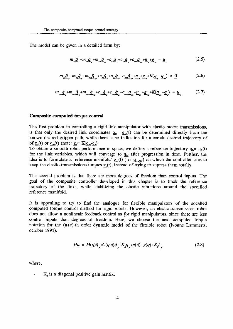
It is appealing to try to find the analogue for flexible manipulators of the socalled computed torque control method for rigid robots. However, an elastic-transmission robot does not allow a nonlineair feedback control as for rigid manipulators, since there are less control inputs than degrees of freedom. Here, we choose the next computed torque notation for the (n+e)-th order dynamic model of the flexible robot (Ivonne Lammerts, October 1991).
where,
- K, is a diagona! positive gain matrix.
4

The composite computed torque control strategy
- e is a chosen reference trajectory of all system variables; in this case, the vector - s= & is a sliding service for 9 according to Asada and Slotine (1986).
- e= a-g is the total error. %= e-9 is the total reference error.
- %= g+& Vtrt,; exto)= e(to). - -
Note, that we do h o w the desired trajectory of the link Variables, ad(t) and its time derivatives, but we haven’t any indication of how to determine a certaindesired trajectory qmd(t) for the elastic motor rotor variables, unless we make use of above computed torque expression in splitting it up again in a partitioned form according to the equations 2.5, 2.6 and 2.7:
u -e sr er mr sr er
= m A + m A + m A +CA +CA + ~ ~ m r + ~ m + ~ m + K @ m r - ~ e ) +K e (2.11)
where K, K, and á, are diagonal, positive definite gain matrices.
With equation (2.10) it is possible to find a reference trajectory for %(t), L ( t ) and L ( t ) . Now it is possible to determine the inputs us(t) and ue(t) with (2.9) and (2.11).
One part of the controller deals with the tracking of a desired trajectory. This part of the controller is in fact a CTC controller. This CTC controller is described by (2.9) and (2.11). The question is: how can we find a reference trajectory of q, +. 9,. The second part of the controller deals with the controlling of elastic vibrations. With (2.10) and q, it is possible to calculate a reference manifold ze,= K(qm-qe,). The second part of the controller stabilizes the elastic vibrations around the specified reference manifold. This part of the controller is in fact also a CTC controller. So, to control a system with flexible transmissions we use a control law which is composed out of two CTC laws. This is the reason why the control law is called the Composite Computed Torque Control law.
5
Controlling the xy table with a C CTC law
3. CONTROLLING THE X Y TABLE WITH A COMPOSITE COMPUTED TORQUE CONTROL LAW
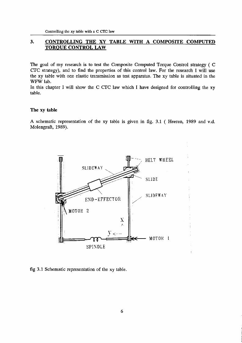
The goal of my research is to test the Composite Computed Torque Control strategy ( C CTC strategy), and to find the properties of this control law. For the research I will use the xy table with one elastic transmission as test apparatus. The xy table is situated in the W e lab. In this chapter I will show the C CTC law which I have designed for controlling the xy table.
The xy table
A schematic representation of the xy table is given in fig. 3.1 ( Heeren, 1989 and v.d. Molengraft, 1989).
-, BELT WHEEL
. . SPINDLE
fig 3.1 Schematic representation of the xy table.

Controlling the xy table with a C C ï C law
For control design we have to choose a suitable model of the xy table. I choose the next model ( v.d. Molengraft, 1989).
fig 3.2 model of the xy table
See appendix A for a more detailed description of the xy table.
The dynamic model of the xy table can be written as:
MïS+CcrLs>S+K~+r~cs> - = Hg
If M,C and & are partitioned in accordance to the partitioning of g, the dynamic model can be given in detailed form (see also appendix A).
7
Controlling the xy table with a C CTC law
The C CTC law
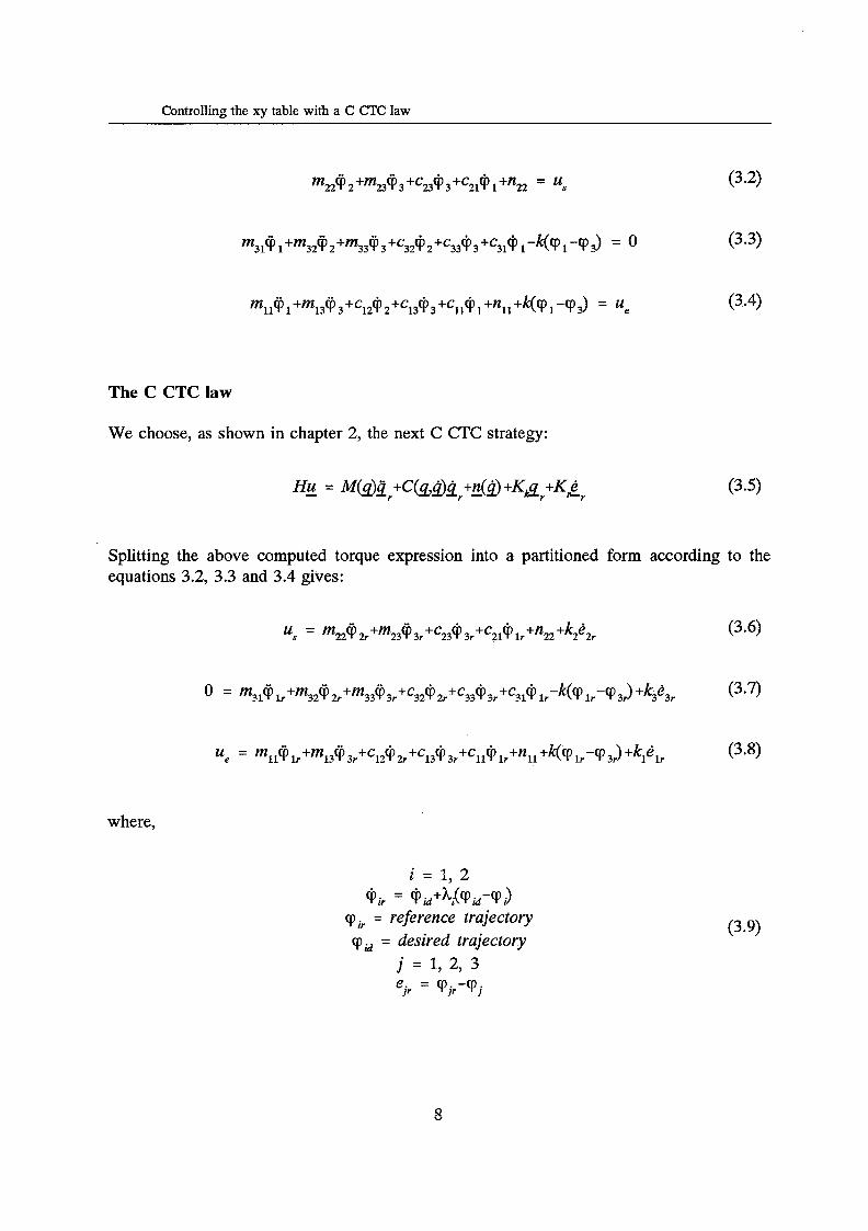
We choose, as shown in chapter 2, the next C CTC strategy:
Splitting the above computed torque expression into a partitioned form according to the equations 3.2, 3.3 and 3.4 gives:
where,
i = 1 , 2 C p v = @pid+hi(cppid-cpi)
cp ir = reference trajectory c p a = desired trajectory
j = 1, 2, 3 e . = cp . -cp
1' I' i
(3.9)
Controlling the xy table with a C CïC law
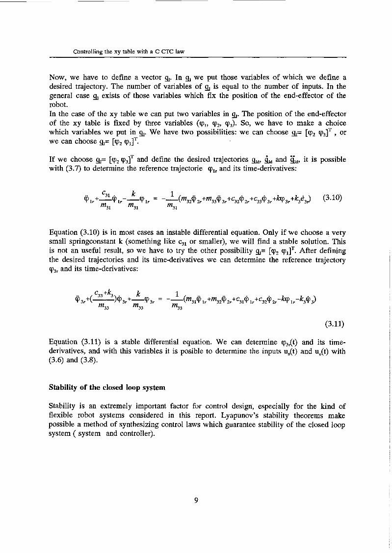
Now, we have to define a vector g,. In g, we put those variables of which we define a desired trajectory. The number of variables of g, is equal to the number of inputs. In the general case % exists of those variables which fix the position of the end-effector of the robot. In the case of the xy table we can put two variables in g,. The position of the end-effector of the xy table is fixed by three variables (qp,, q),, qpJ. So, we have to make a choice which variables we put in g,. We have two possibilities: we can choose g,= [cp2 cp3IT , or we can choose g,= [cp2 cpllT.
If we choose g,= [r.p2cp3]T and define the desired trajectories sd, i d and &, it is possible with (3.7) to determine the reference trajectorie cplr and its time-derivatives:
Equation (3.10) is in most cases an instable differential equation. Only if we choose a very small springconstant k (something like ~ 3 1 or smaller), we will find a stable solution. This is not an usehl result, so we have to try the other possibility g,= [qp, vilT. After defining the desired trajectories and its time-derivatives we can determine the reference trajectory cp3r and its time-derivatives:
(3.11)
Equation (3.11) is a stable differential equation. We can determine cp3Xt) and its time- derivatives, and with this variables it is posible to determine the inputs us(t) and u,(t) with (3.6) and (3.8).
Stability of the closed loop system
Stability is an extremely important factor for control design, especially for the kind of flexible robot systems considered in this report. Lyapunov's stability theorems make possible a method of synthesizing control laws which guarantee stability of the closed loop system ( system and controller).
9
Controlling the xy table with a C CTC law
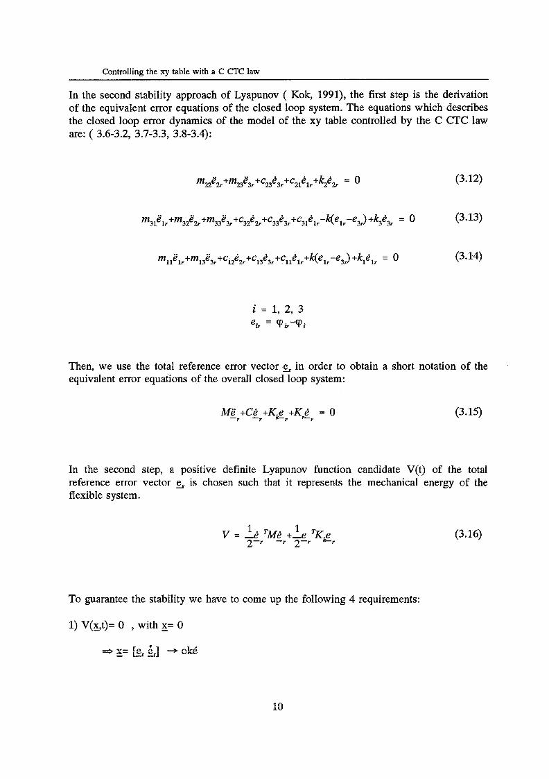
In the second stability approach of Lyapunov ( Kok, 1991), the first step is the derivation of the equivalent error equations of the closed loop system. The equations which describes the closed loop error dynamics of the model of the xy table controlled by the C CïC law are: ( 3.6-3.2, 3.7-3.3, 3.8-3.4):
m22ë2r+m23ë3r +cue3r+c21elr+k2è2r = 0
mllëlr+m13ë3r+~12e2r+~13e3r+~11~lr+k(~lr-~3$ +kidlr = 0
/3 I - \ (3.1L)
(3.13)
(3.14)
i = 1, 2, 3 e, = rp,-rpi
Then, we use the total reference error vector e, in order to obtain a short notation of the equivalent error equations of the overall closed loop system:
Më +Ce +Kgr+KC = O (3.15) -r -r +r
In the second step, a positive definite Lyapunov function candidate V(t) of the total reference error vector e, is chosen such that it represents the mechanical energy of the flexible system.
V = -e 1 'Me +-e 1 'Kg, 2-r -r 2-r (3.16)
To guarantee the stability we have to come up the following 4 requirements:
1) V(st)= O , with g= O
=9 - x= h&] + oké

Controlling the xy table with a C CTC law
2) V(E7t)r 4lxll => The inertia matrix M is positive definite and I(k is not negative definite. 4 oké
3) V(st)= continuous and differentiable.
4 oké
4) V(5t) c o
=> With (3.16) we can find:
1 V = e 'Më +,e 'Ah2 +e 'Kk e -r -r 2 - r -r -r -r
With (3.15) can be given by:
(3.17)
(3.18)
I have defined the matrix C (see appendix A) such that the matrix [MM-C] is skew-symmetric, i.e.:
[&-Cl 1 = -[-M-C]' 1 2 2
(3.19)
. As a consequence, we can make use of the property of skew-symmetry of [%M-C] in that:
xT[-i@-C]X 1 = O , for any arbritrary - 2
(3.20)
Controlling the xy table with a C CTC law
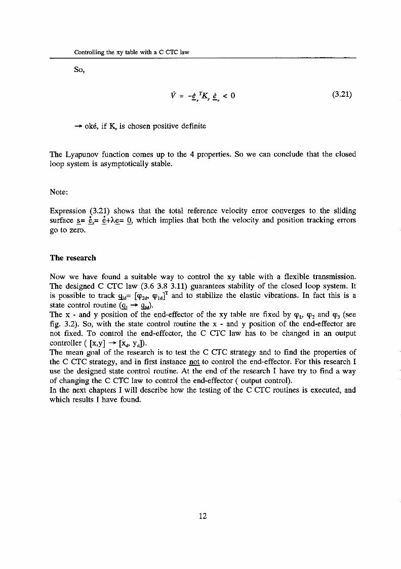
so,
Y = -e 'Kr e < O -r -r
(3.21)
+ oké, if it4 is ~hosen positive definite
The Lyapunov function comes up to the 4 properties. So we can conclude that the closed loop system is asymptotically stable.
Note:
Expression (3.21) shows that the total reference velocity error converges to the sliding surface E= &= - - ;+he= 0, which implies that both the velocity and position tracking errors go to zero.
The research
Now we have found a suitable way to control the xy table with a Bexible transmission. The designed C CTC law (3.6 3.8 3.11) guarantees stability of the closed loop system. It is possible to track a d = [vu, v i d l T and to stabilize the elastic vibrations. In fact this is a state control routine @1 + $2. The x - and y position of the end-effector of the xy table are fixed by cpl, cp2 and ip3 (see fig. 3.2). So, with the state control routine the x - and y position of the end-effector are not fixed. To control the end-effector, the C CTC law has to be changed in an output controller ( [x,y] + [xd, yd]). The mean goal of the research is to test the C CTC strategy and to find the properties of the C CTC strategy, and in first instance not to control the end-effector. For this research P use the designed state control routine. At the end of the research I have try to find a way of changing the C CTC law to control the end-effector ( output control). In the next chapters I will describe how the testing of the C CTC routines is executed, and which results I have found.
12
Properties of the C CTC strategy
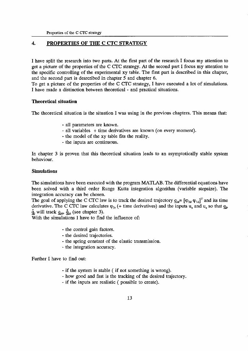
4. PROPERTIES OF THE C CTC STRATEGY
I have split the research into two parts. At the first part of the research I focus my attention to get a picture of the properties of the C CTC strategy. At the second part I focus my attention to the specific controlling of the experimental xy table. The first part is described in this chapter, and the second part is desrcribed in chapter 5 and chapter 6. To get a picture of the properties of the C C ï C strategy, I have executed a lot of simulations. I have made a distinction between theoretical - and practical situations.
Theore tical situation
The theoretical situation is the situation I was using in the previous chapters. This means that:
- all parameters are known. - all variables + time derivatives are known (on every moment). - the model of the xy table fits the reality. - the inputs are continuous.
In chapter 3 is proven that this theoretical situation leads to an asymptotically stable system behaviour.
Simulations
The simulations have been executed with the program MATLAB. The differential equations have been solved with a third order Runge Kutta integration algorithm (variable stepsize). The integration accuracy can be chosen. The goal of applying the C CTC law is to track the desired trajectory [cpzd (pidlT and its time derivative. The C CTC law calculates q~~~ (+ time derivatives) and the inputs u, and u, so that $,
With the simulations I have to find the influence of: will track qld, &d (see chapter 3).
- the control gain factors. - the desired trajectories. - the spring constant of the elastic transmission. - the integration accuracy.
Further I have to find out:
- if the system is stable ( if not something is wrong). - how good and fast is the tracking of the desired trajectory. - if the inputs are realistic ( possible to create).
13
Properties of the C CTC strategy
Simulation results theoretical situations
In this paragraph I will show and discuss the most important simulation results.
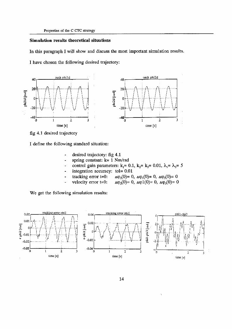
I have chosen the following desired trajectory:
CI - '3 1 ii
.- 3. 3 - Y
il. Y
= - c. c
O 1 2 3
time [s] time [s]
fig 4.1 desired trajectory
I define the following standard situation:
- desired trajectory: fig 4.1 - - - integration accuracy: tol= 0.01 - tracking error t=O: ~cp,(O)= O, ~cp,(O)= O, acp,(O)= O - velocity error t=O: ~cp,(O)= O, ~cpl(O)= O, ~ c p ~ ( O ) = O
spring constant: k= 1 Nm/rad control gain parameters: k,= 0.1, k2= k3= 0.01, hl= &= 5
We get the following simulation results:
tracking error phi2 0.02 1 0.04 r tracking error phi1 phi i-ohi3 1
-0.03 O 1 2 3
time [s]
-0.04 ' 1 O 1 2 3
time [SI
I
0 1 I 3 time [s]
14
Properties of the C CTC strategy
input< 30- trackine error duhi2
. . . . . ....
-20 7 O 1 2 3 O 1 2 3 o 1 - 3
time [SI time [s] time [s] ~
dphi3-dphi3r 0.6 i I
phi3 and phi3r
-40 ' 1 -0.4 ' I 0 1 2 3 O 1 2 3
time [s] time [SI
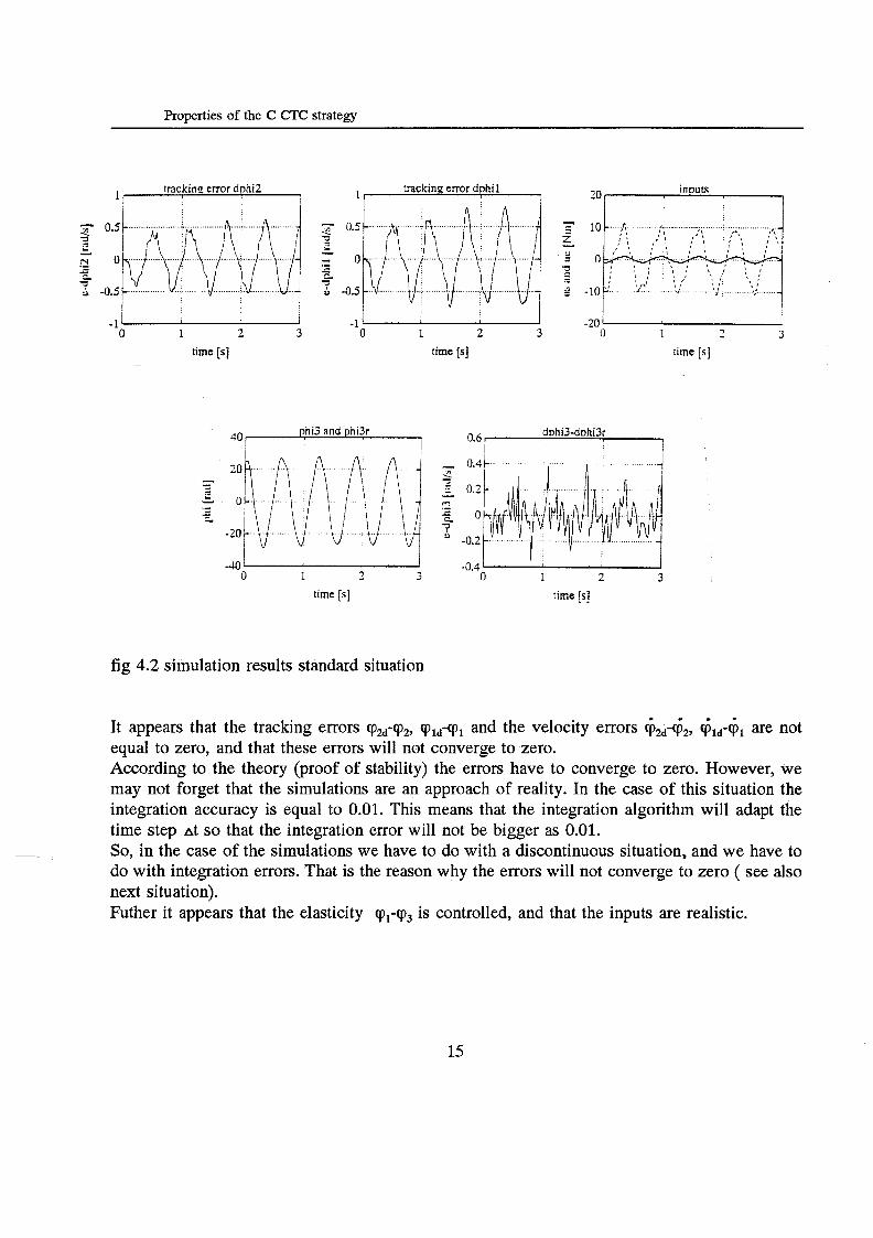
fig 4.2 simulation results standard situation
It appears that the tracking errors cpZd-cpZ, cpld-91 and the velocity errors &d-&, (P ld-61 are not equal to zero, and that these errors will not converge to zero. According to the theory (proof of stability) the errors have to converge to zero. However, we may not forget that the simulations are an approach of reality. In the case of this situation the integration accuracy is equal to 0.01. This means that the integration algorithm will adapt the time step At so that the integration error will not be bigger as 0.01. So, in the case of the simulations we have to do with a discontinuous situation, and we have to do with integration errors. That is the reason why the errors will not converge to zero ( see also next situation). Futher it appears that the elasticity cpi-cp3 is controlled, and that the inputs are realistic.
15
Properties of the C CTC strategy
20 5 5,
IO-.. ?;.. 'L I.. ; .._,..............,. . a t ~ , /', :';-
, I I I I $ , ' % : :
5; . . .... ..,~. . .............:..~ ......... 1.1 .......,
; , I 3 , I
,~ I < * > I < f s 8
' I % . . . . . . . . . . . 0 -* : : ' ............... I < ~ , , L ( <.: , I . i '. ; .; ....................... ~ ..................._
- I ( ) 2 -
Now I will change one or some aspects of the presented standard situation. I will consider the influence of the changed aspects.
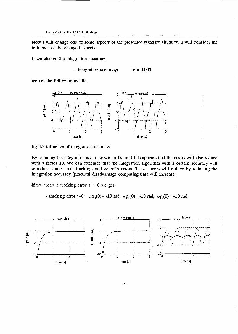
If we change the integration accuracy:
- integration accuracy: tol= 0.001
we get the following results:
- -70
- xlO-3 tr. error phi2 , xlO-3 tr. error phil - 1
time [SI time [s]
fig 4.3 influence of integration accuracy
By reducing the integration accuracy with a factor 10 its appears that the errors will also reduce with a factor 10. We can conclude that the integration algorithm with a certain accuracy will introduce some small tracking- and velocity errors. These errors will reduce by reducing the integration accuracy (practical disadvantage computing time will increase).
If we create a tracking error at t=O we get:
- tracking error t=O: ~ c p , ( O ) = -10 rad, ~rp,(O)= -10 rad, A C ~ ~ ( O ) = -10 rad
16
Properties of the C CTC strategy
Li
......................... ..............
s 1 -20 .....................................
-30 O 1 3 O 1 2 3
time Is] time [SI
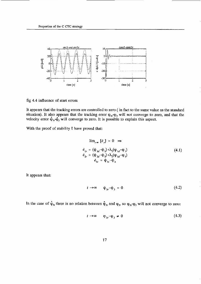
fig 4.4 influence of start errors
It appears that the tracking errors are controlled to zero ( in fact to the same value as the standard situation). It also appears that the tracking error cp3;cp3 will not converge to zero, and that the velocity error G3;(j3 will converge to zero. It is possible to explain this aspect.
With the p ~ ~ f of stability I have proved that:
lim, [er] = O -
It appears that:
In the case of $3r there is no relation between 63r and cp3, so ~ p ~ ~ - c p , will not converge to zero:
t + m ~ p 3 r - ~ p 3 * 0 (4.3)
17
Properties of the C CTC strategy
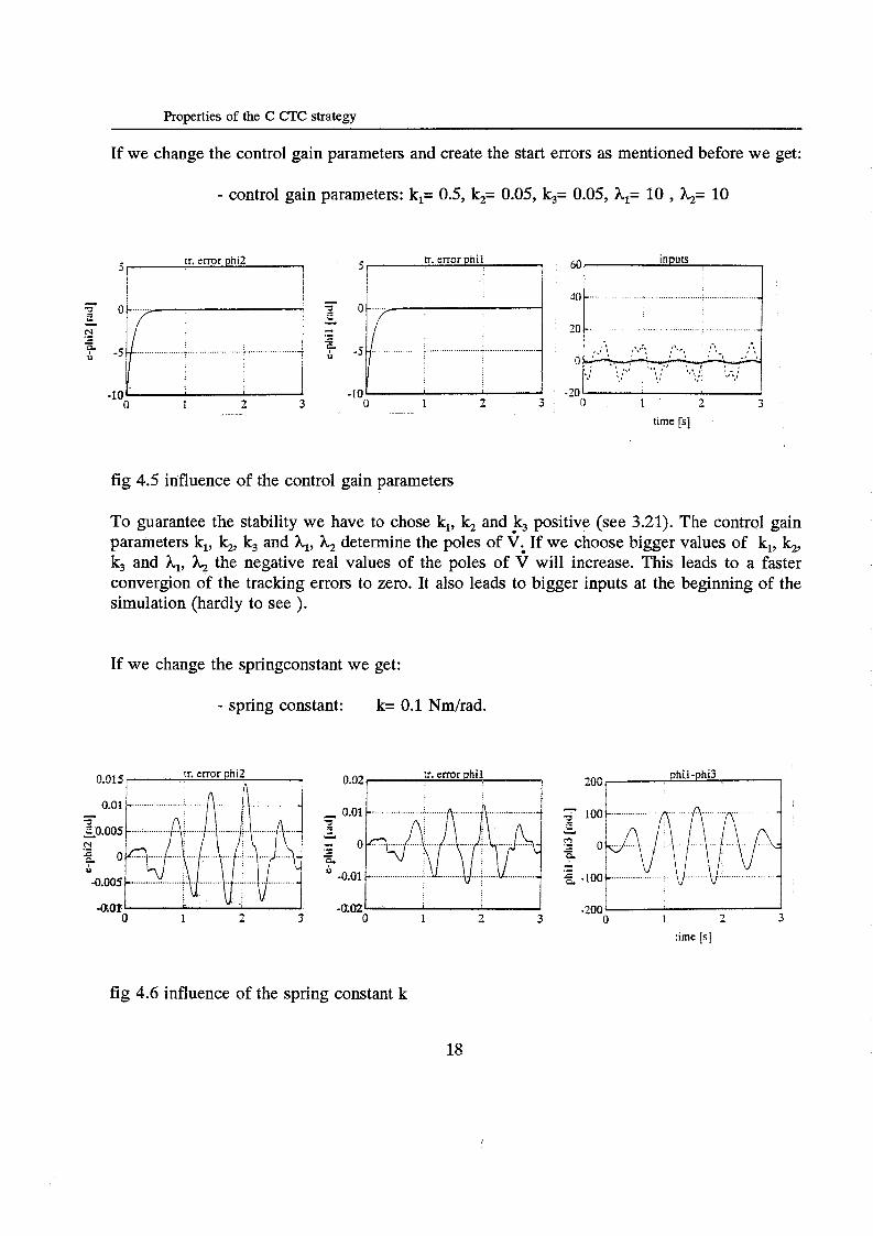
If we change the control gain parameters and create the start errors as mentioned before we get:
- control gain parameters: k,= 0.5, k,= 0.05, k3= 0.05, A,= 10 , &= 10
7 tr. error Phil 5 tr. error phi2 5
N
a .- - : j -5 0~~~ f -//-j
-10 O 1 2 3 o 1 2 3 o 1 2 3
~
-IO
time p]
fig 4.5 influence of the control gain parameters
To guarantee the stability we have to chose k,, k, andk, positive (see 3.21). The control gain parameters k,, k,, k, and A,, h, determine the poles of V. If we choose bigger values of k,, k,, k3 and A,, A, the negative real values of the poles of ? will increase. This leads to a faster convergion of the tracking errors to zero. It also leads to bigger inputs at the beginning of the simulation (hardly to see ).
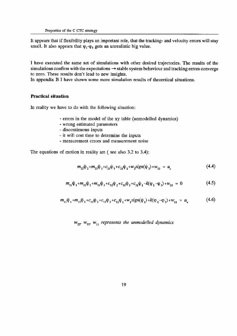
If we change the springconstant we get:
- spring constant: k= 0.1 Nm/rad.
tr. error phi2 0.015 I tr. error phi1 0.02
O 1 2 3
phil-phi3 200
I 3
-200' O 1 7
time [s]
fig 4.6 influence of the spring constant k
18
Properties of the C CTC strategy
It appears that if flexibility plays an important role, that the tracking- and velocity errors will stay small. It also appears that cpl-cp3 gets an unrealistic big value.
I have executed the same set of simulations with other desired trajectories. The results of the simulations confirm with the expectations -., stable system behaviour and tracking errors converge to zero. These results don't iead to new insights. In appendix B I have shown some more simulation results of theoretical situations.
Practical situation
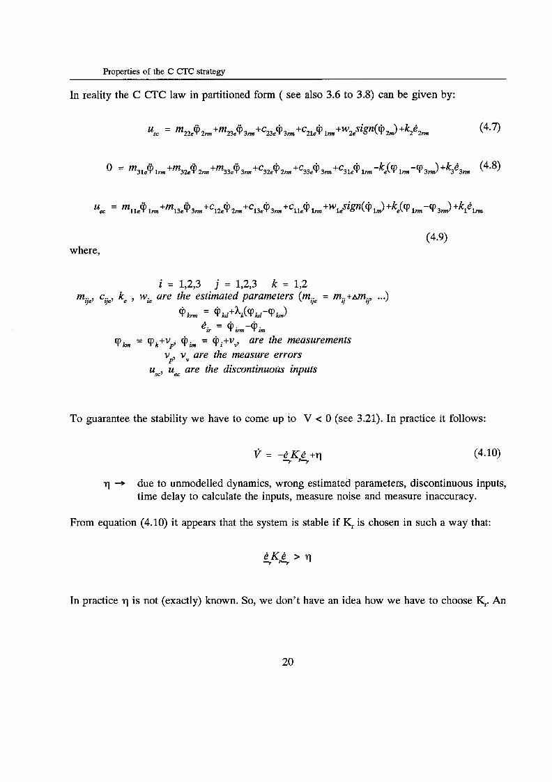
In reality we have to do with the following situation:
- errors in the model of the xy table (unmodelled dynamics) - wrong estimated parameters - discontinuous inputs - it will cost time to determine the inputs - measurement errors and measurement noise
The equations of motion in reality are ( see also 3.2 to 3.4):
w227 w339 wll represents the unmodelled dynamics
19
Properties of the C CTC strategy
In reality the C CïC law in partitioned form ( see also 3.6 to 3.8) can be given by:
(4.9) where,
i = 1,2,3 j = 1,2,3 k = 1,2 mie, cie, I&, , wk are the estimated parameters (mie = m..+m. ...)
11 YY
@,, = @kd+'k(T,-(Pd
e, = +. urn -q - im qb = 'Pk+vp, @h = Cpi+vG are the measurements
vp7 vy are the measure errors u,,, u,, are the discontinuous inputs
To guarantee the stability we have to come up to V e O (see 3.21). In practice it follows:
Y = - d K è +q -r r-r
(4.10)
q + due to unmodelled dynamics, wrong estimated parameters, discontinuous inputs, time delay to calculate the inputs, measure noise and measure inaccuracy.
From equation (4.10) it appears that the system is stable if M, is chosen in such a way that:
In practice q is not (exactly) known. So, we don't have an idea how we have to choose &. An
20
Properties of the C CTC strategy
other problem is that in practice we can’t choose y too big because of the fact that the inputs u, and u, will grow to unrealistic values (in practice the inputs are bounded).
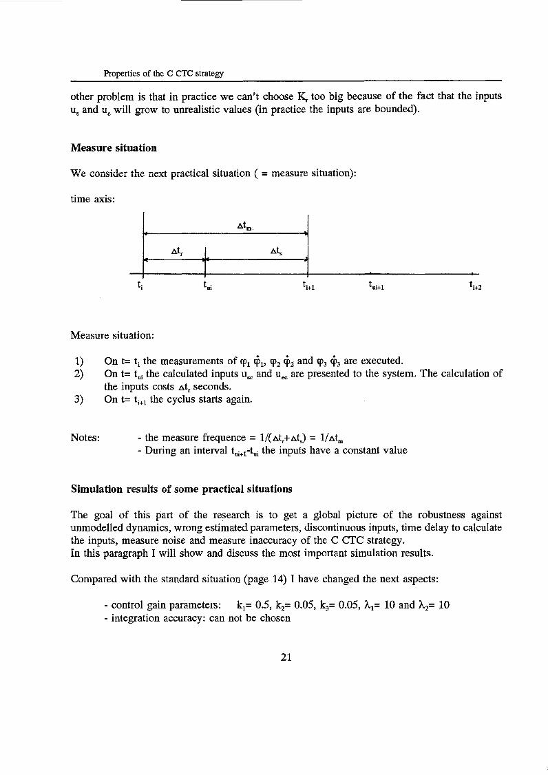
Measure situation
We consider the next practica! situation ( = measure sitriation):
time axis:
Measure situation:
1) 2)
3)
On t= ti the measurements of rp, Ce,, (p2 G2 and ip3 G3 are executed. On t= t, the calculated inputs u, and u, are presented to the system. The calculation of the inputs costs Atr seconds. On t= ti+, the cyclus starts again.
Notes: - the measure frequence = l/(Atr+atJ = l/at, - During an interval tui+& the inputs have a constant value
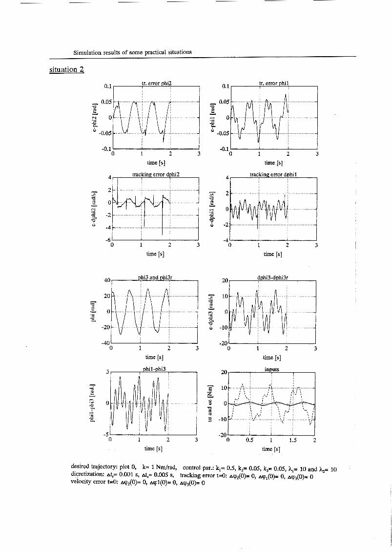
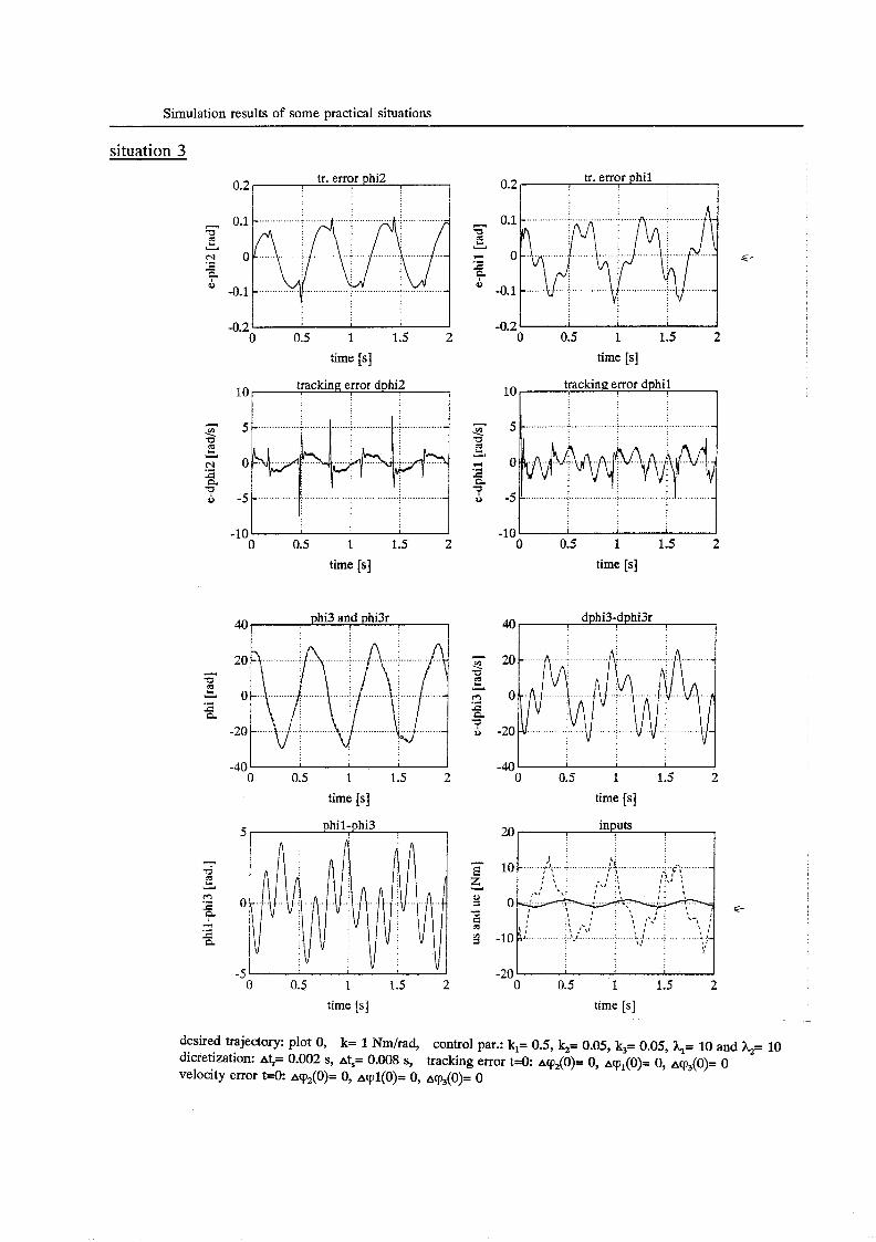
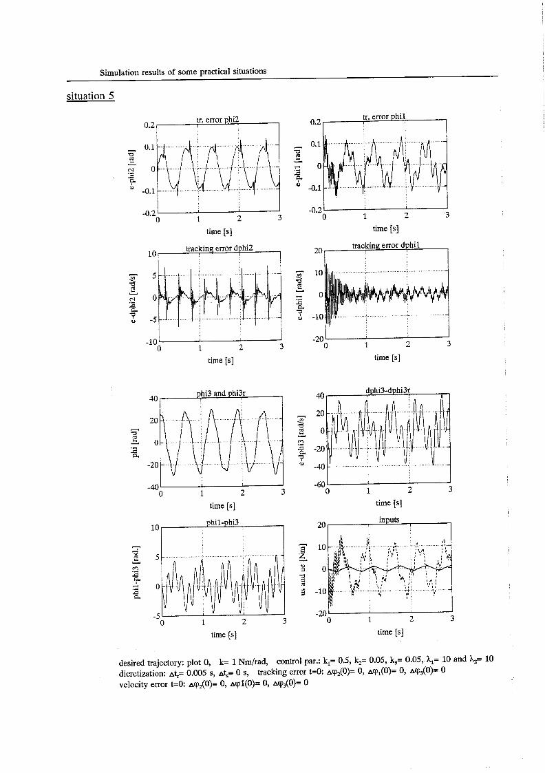
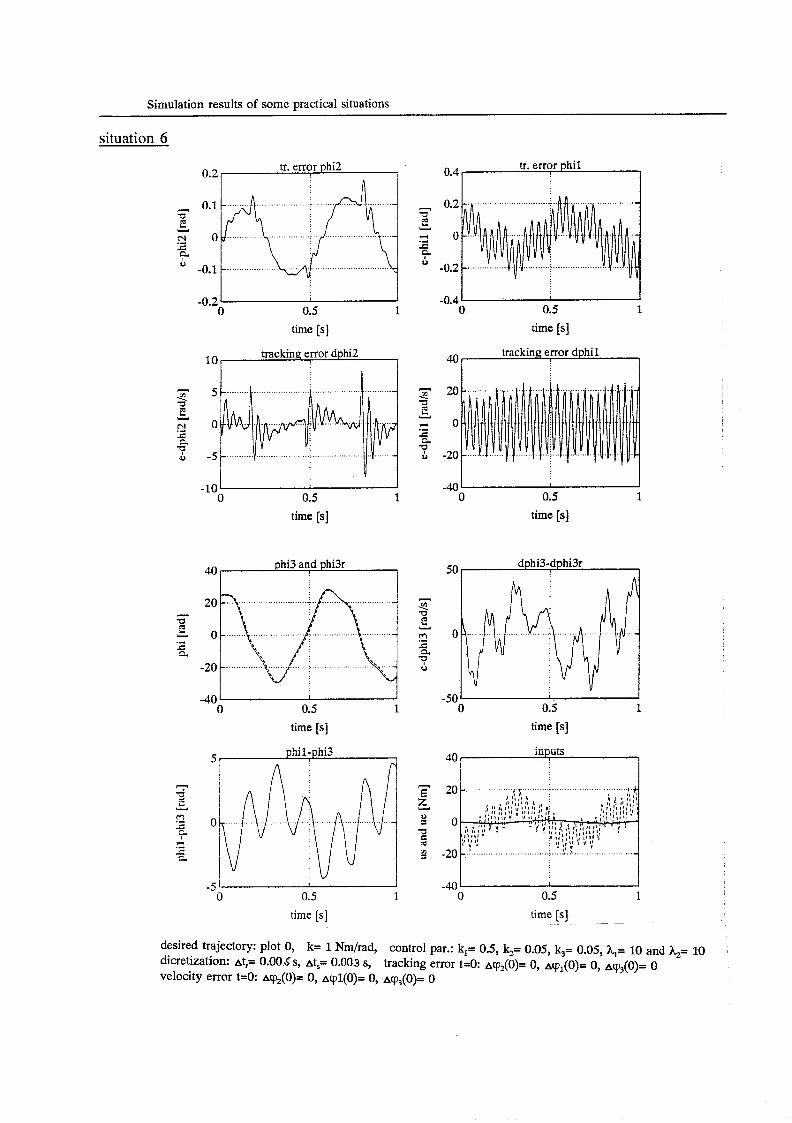
§imps!sptiunn results of some practical situations
The goal of this part of the research is to get a global picture of the robustness against unmodelled dynamics, wrong estimated parameters, discontinuous inputs, time delay to calculate the inputs, measure noise and measure inaccuracy of the C C ï C strategy. In this paragraph I will show and discuss the most important simulation results.
Compared with the standard situation (page 14) I have changed the next aspects:
- control gain parameters: - integration accuracy: can not be chosen
k,= 0.5, k2= 0.05, k3= 0.05, hl= 10 and h2= 10
21
Properties of the C CTC strategy
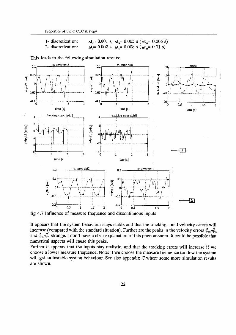
1- discretization: Atr= 0.001 S, Ats= 0.005 S (Atm= 0.006 S)
2- discretization: Att,= 0.002 s, AtSZ 0.008 s (At,= 0.01 s)
This leads to the following simulation results:
.................... e 10 ........ I'. ..................... l ................... * .....
- 0
............
.- .- c
-0.1 ' 1 O 1 2 3
time [s]
O 1 2 3 time [SI
-20 u 1 2 3 o 0.5 1 1.5 2
-0.1 - O
time {SI trackhe emr duhil 4 , I
time [s]
tr. error hi2 0.2
0 1 i- .................... .'._.._.
-0.2 o 0.5 1 1.5 2 o 0.5 I 1.5 2
fig 4.7 Influence of measure frequence and discontinuous inputs
It appears that the system behaviour stays stable and that the tracking -
time [SI
and velocity errors will increase (compared with the standard situation). Further are the peaks in the velocity errors &-& and strange. I don't have a clear explanation of this phenomenom. It could be possible that numerical aspects will cause this peaks. Further it appears that the inputs stay realistic, and that the tracking errors will increase if we choose a lower measure frequence. Note: if we choose the measure frequence too low the system will get an instable system behaviour. See also appendix C where some more simulation results are shown.
22
Properties of the C CTC strategy
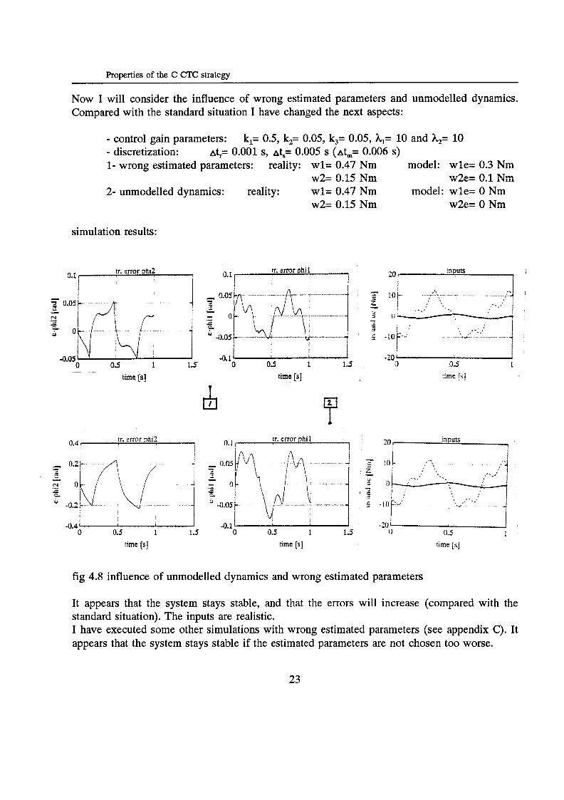
Now I will consider the influence of wrong estimated parameters and unmodelled dynamics. Compared with the standard situation I have changed the next aspects:
- control gain parameters:
1- wrong estimated parameters: reality: wl= 0.47 Nm model: wle= 0.3 Nm w2e= 0.1 Nm
2- unmodelled dynamics: reality: wl= 0.47 Nm model: wle= O Nm w2e= O Nm
k,= 0.5, k2= 0.05, k,= 0.05, hl= 10 and A,= 10 - discretization: At,= 0.001 S , Att,= 0.005 S (Atm= 0.006 s)
w2= 0.15 Nm
w2= 0.15 Nm
simulation results:
tr. error phi2 0.1 r I I
tr. error Phil 0.1 r i 20, ?
0 0.5 1 15 o . 0 5 15 ~~
time [SI time [s]
n - , ,- , I .
\ ,. * - -10 F..:. .. . ... ..~.. . . . ..... .... .
inputs 1 0.4 1 1 20 f tr. error phi1 0.1, [r. error phi2
I
I i - 0.21
.- - 9
-0.2 ’
-0.4 O 0.5 1 1.5
! 1 0.5 1
time [s] time [SI time [b]
fig 4.8 influence of unmodelled dynamics and wrong estimated parameters
It appears that the system stays stable, and that the errors will increase (compared with the standard situation). The inputs are realistic. I have executed some other simulations with wrong estimated parameters (see appendix C). It appears that the system stays stable if the estimated parameters are not chosen too worse.
23
Properties of the C C ï C strategy
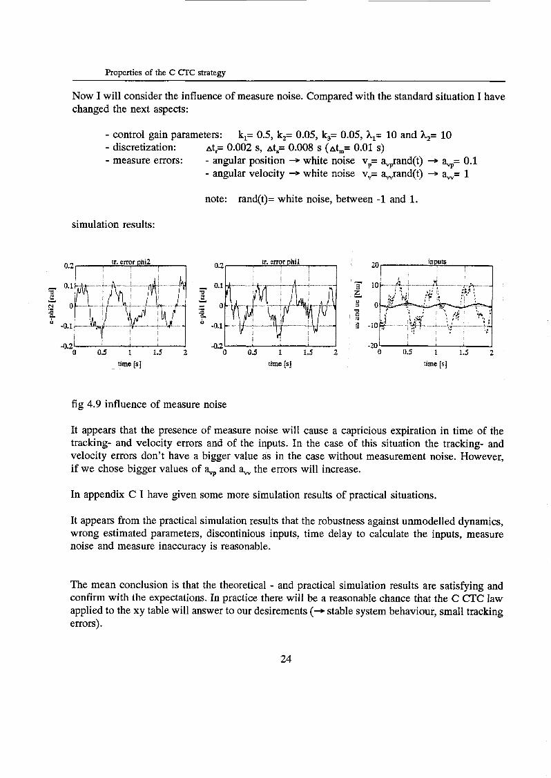
Now I will consider the influence of measure noise. Compared with the standard situation I have changed the next aspects:
- control gain parameters:
- measure errors:
k,= 0.5, k2= 0.05, k3= 0.05, hl= 10 and &= 10
- angular position + white noise vp= %rand(t) + a+ 0.1 - angular velocity + white noise vv= uand( t )
- discretization: Atr= 0.002 S , Ats= 0.008 s (Atm= 0.01 S )
%= 1
note: rand(t)= white noise, between -1 and 1.
simulation results:
o 0.5 1 1.5 2 O O 5 1 1.5 2 o 0.5 1 1.5 2 time [SI time [SI time is]
fig 4.9 influence of measure noise
It appears that the presence of measure noise will cause a capricious expiration in time of the tracking- and velocity errors and of the inputs. In the case of this situation the tracking- and velocity errors don't have a bigger value as in the case without measurement noise. However, if we chose bigger values of and a, the errors will increase.
In appendix C I have given some more simulation results of practical situations.
It appears from the practical simulation results that the robustness against unmodelled dynamics, wrong estimated parameters, discontinious inputs, time delay to calculate the inputs, measure noise and measure inaccuracy is reasonable.
The mean conclusion is that the theoretical - and practical simulation results are satisfying and confirm with the expectations. In practice there will be a reasonable chance that the C CTC law applied to the xy table will answer to our desirements (+ stable system behaviour, small tracking errors).
24

Applying of the C CTC controller to the xy table
5. APPLYING OF THE CTC CONTROLLER TO THE XY TABLE
Now that we have a good picture of the properties of the controlled system we can focus our attention to the specific controlling of the xy table. This is the second part of the research.
The total system
In chapter 3 and appendix A I have shown a schematic representation of the xy table. In this paragraph I will give some more details of the measure- and control system of the xy table (see fig 5.1).
im
! i][- !
S L I D E W A Y , - BELT WHEEL /’
k&& M O T O R 1
fig 5.1 Schematic representation of the total system.
25
Applying of the C CTC controller to the xy table
The designed control routine has been put in the computer. The inputs of the control routine are the measurements of the angular positions (pi, cp2 and cp3. The outputs are the by the control routine calculated small electrical currents. Before the currents are presented to the motors they are amplified. Depending on these electrical currents the motors deliver certain torques. These torques are the inputs of the system (us and uJ. For the total organisation of executing experiments I have the avaliability of the new software designed by Jos Banens ( member of the WFW group). This software is written in "C". The big advantage of using this software is that it is build up in standard routines and that the programs can communicate with Matlab programs.
The total system has its limitations. The most important ones are:
-
- Inaccuracy of the amplifier. - -
The calculated inputs are clipped (are bounded) on a certain positive and negative value. This to protect the amplifier and the motors.
The elasticity of the xy table is restricted. It appears that max Icpi-cp3 I = I 3 rad. The computing time. It will cost time to calculate the inputs. The computing time may not be too big (see chapter 4). Inaccuracy of the measurements. The measurements of the angular position do have a certain inaccuracy. Curved axis (y direction) of the "y table.
-
-
Implementation of the C CTC controller
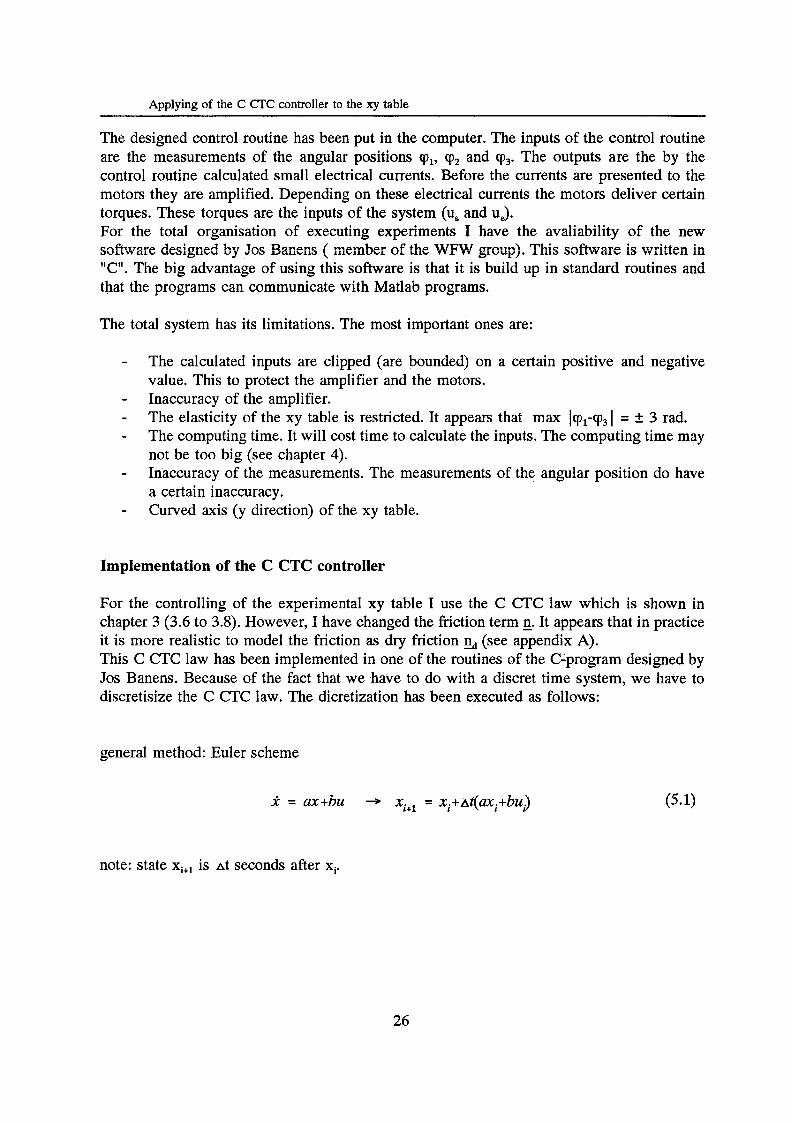
For the controlling of the experimental xy table I use the C C ï C law which is shown in chapter 3 (3.6 to 3.8). However, I have changed the friction term n. It appears that in practice it is more realistic to model the friction as dry friction This C CTC law has been implemented in one of the routines of the C-program designed by Jos Banens. Because of the fact that we have to do with a discret time system, we have to discretisize the C CTC law. The dicretization has been executed as follows:
(see appendix A).
general method: Euler scheme
X = a+bü + xi+i = xi+at(axi+bu;)
note: state xi+l is At seconds after xi.
26

Applying of the C CïC controller to the xy table
The reference trajectories:
(3, 3ri+1 = (3, 3ri +A@ 3ri
For the calculation of the reference trajectories and the inputs, we need:
1. 2. 3. 4.
desired trajectories cpld, cp2d (can be chosen) estimated system parameters (see appendix A) control gain parameters (can be chosen) the angular position and angular velocities (cpl, cp2, cp3, &, G2 and G3)
The first two points needs no further discussion. The third point about the control gain parameters needs a short explanation. As shown in chapter 3 (proof of stability) and chapter 4 the control gain parameters do partitial fix the poles o f ? (see 4.10):
If the poles of V have negative real values, the system is stable. Because of the fact that y is not known we have to find suitable control gain parameters by executing simulations and experiments.
27
Applying of the C CTC controller to the xy table
Note: the control gain parameters can't be chosen too big, because of the fact that the inputs are clipped on certain values. This clipping of the inputs can lead to undesired system behaviour. The fourth point deals with the handling of the measurements. As already written, the angular positions cpl , cp2 and cp3 are measured. Out of these measurements and out of the (partial) known system behaviour we have to estimate the angular velocities &, G2 and (p3. In other terms, we have to design an observer algorithm for the reconstruction of the angular velocities. In appendix D I have designed such an algorithm.
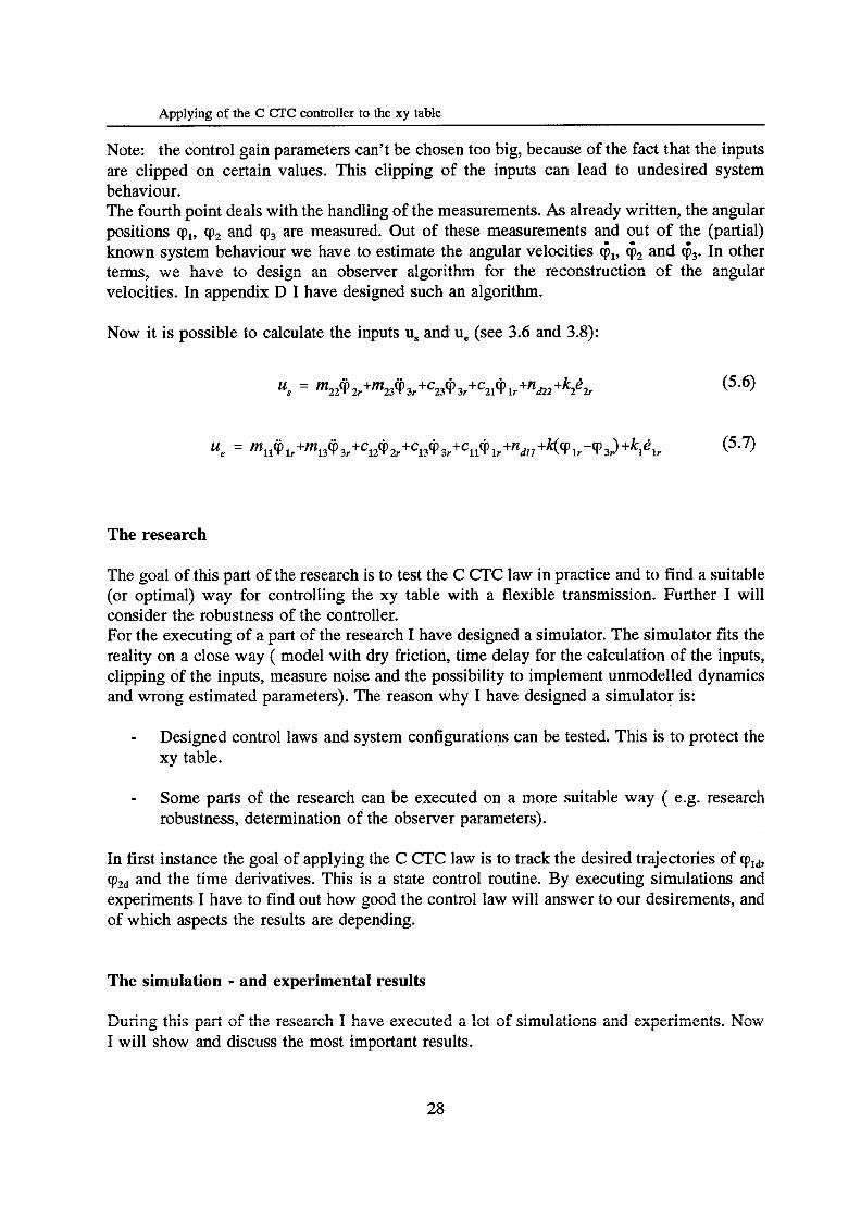
Now it is possible to calculate the inputs u, and u, (see 3.6 and 3.8):
The research
The goal of this part of the research is to test the C CTC law in practice and to find a suitable (or optimal) way for controlling the xy table with a flexible transmission. Further I will consider the robustness of the controller. For the executing of a part of the research I have designed a simulator. The simulator fits the reality on a close way ( model with dry friction, time delay for the calculation of the inputs, clipping of the inputs, measure noise and the possibility to implement unmodelled dynamics and wrong estimated parameters). The reason why I have designed a simulator is:
- Designed control laws and system configurations can be tested. This is to protect the xy table.
- Some parts of the research can be executed on a more suitable way ( e.g. research robustness, determination of the observer parameters).
In first instance the goal of applying the C CTC law is to track the desired trajectories of cpId, cp2d and the time derivatives. This is a state control routine. By executing simulations and experiments I have to find out how good the control law will answer to our desirements, and of which aspects the results are depending.
The simulation - and experimental results
During this part of the research I have executed a lot of simulations and experiments. Now I will show and discuss the most important results.
28
Applying of the C CTC controller to the xy table
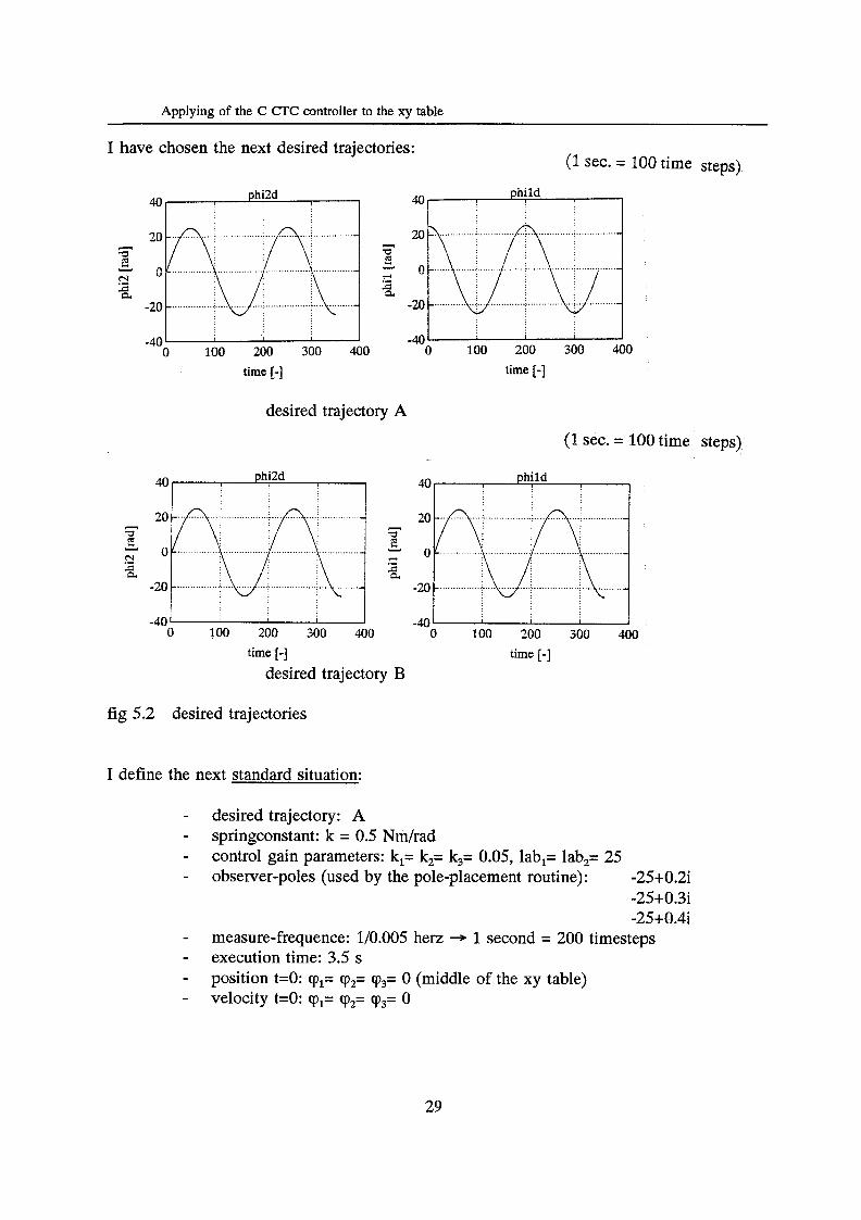
I have chosen the next desired trajectories:
ü
O 100 200 300 400 O 100 200 300 400 time [-3 time [-I
-40
desired trajectory A
(1 sec. = 100 time steps)
phild 40 phi2d 40
a
, -40 -40 I
O 100 200 300 400 O 100 200 300 400 time [-] time [-I
desired trajectory B
fig 5.2 desired trajectories
i define the next standard situation:
desired trajectory: A springconstant: k = 0.5 Nm/rad control gain parameters: k,= k2= k3= 0.05, lab,= lab,= 25 observer-poles (used by the pole-placement routine) : -25+0.21
-25+0.3i -25+0.4i
measure-frequence: l/0.005 herz + 1 second = 200 timesteps execution time: 3.5 s position t=O: (pi= cp2= cp3= O (middle of the xy table) velocity t=O: cpl= cp2= cp3= O
29

Applying of the C CTC controller to the xy table
200
-
- - -
The simulation results are:
;: ; :
-4 -20
-6 -30 O 200 400 600 800
time [-I time [-I
400 100 -
: :, y 200 -
.- m O -
F -200 -
- 2 u
c c. -
-50 -400
tr. error dphi2 100 I
y:/, , , I .c a 0 -50
-100 O 200 400 600 800
time [-I time [-]
-4 ‘ 1 O 200 400 600 800
time [-I
inputs 4000
-4000 ‘ O 200 400 600 800
time [-I
fig 5.3 simulation results standard situation
It appears that the simulation results are good. The system stays stable and the tracking - and velocity errors converge to zero (to small values). At the first part of the simulation the controller has to control the start errors to zero. This leads to big control actions. It appears that the by the control routine calculated inputs u, and u, are clipped. In this case the dipping of the inputs doesn’t lead to undesired system behaviour.
30
Applying of the C CTC controller to the xy table
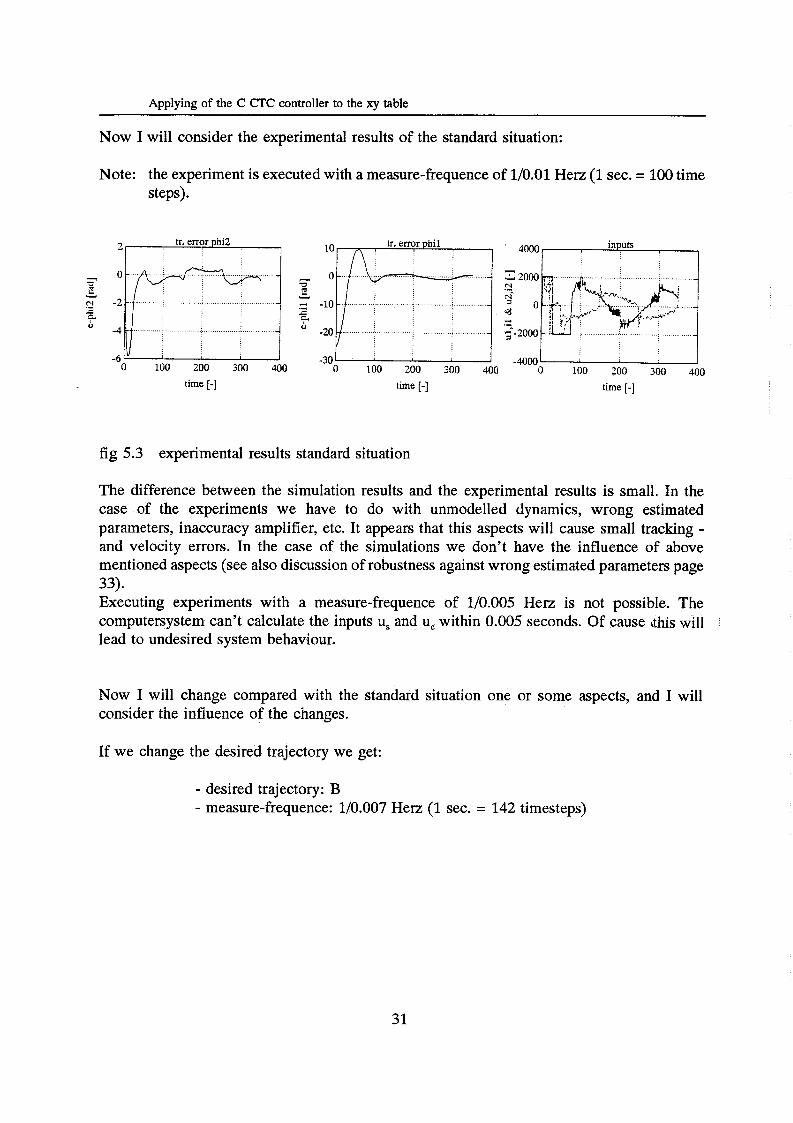
Now I will consider the experimental results of the standard situation:
Note: the experiment is executed with a measure-frequence of 1/0.01 Herz (1 sec. = 100 time steps).
tr- error phi2 tr. exo: phi1 2
E
D- y -4
Y
.c
-20
-6 -30 O 100 200 300 400 o 100 200 300 4oa O 100 200 300 400
time [-I time [-] time [-I
fig 5.3 experimental results standard situation
The difference between the simulation results and the experimental results is small. In the case ~f the experiments we have to do with unmodelled dynamics, wrong estimated parameters, inaccuracy amplifier, etc. It appears that this aspects will cause small tracking - and velocity errors. In the case of the simulations we don’t have the influence of above mentioned aspects (see also discussion of robustness against wrong estimated parameters page
Executing experiments with a measure-frequence of 1/0.005 Herz is not possible. The computersystem can’t calculate the inputs u, and u, within 0.005 seconds. Of cause ithis will lead to undesired system behaviour.
33).
Now I will change compared with the standard situation one or some aspects, and I will consider the influence of the changes.
If we change the desired trajectory we get:
- desired trajectory: B - measure-frequence: 1/0.007 Hen (1 sec. = 142 timesteps)
31
Applying of the C CTC controller to the xy table
1
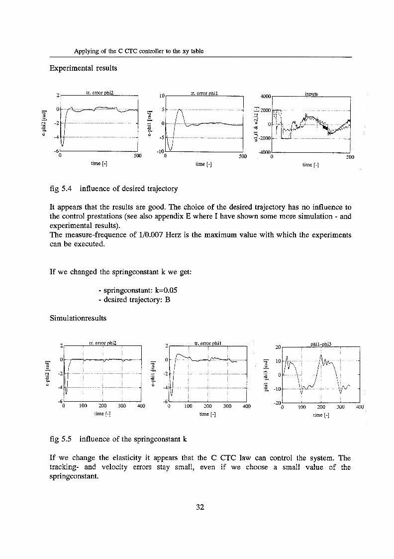
Experimental results
2 20
- - O - O L! u - - 5 - 2 - - - - - -
y -4 - ? -4. - I
ir -6 -6 -20
tr. error phi2 2
0 ...........................................
-2 l m ..........................................
i w ................................................................ -4
-6 I O 500
time [-I time [-I
inputs 4000
-4000 O 500
time [-I
fig 5.4 influence of desired trajectory
It appears that the results are good. The choice of the desired trajectory has no influence to the control prestations (see also appendix E where I have shown some more simulation - and experimental results). The measure-frequence of 1/0.007 Herz is the maximum value with which the experiments can be executed.
If we changed the springconstant k we get:
- springconstant: k=0.05 - desired trajectory: B
Simulationresults
fig 5.5 influence of the springconstant k
If we change the elasticity it appears that the C CTC law can control the system. The tracking- and velocity e ~ ~ c r s stzy smzll, even if we choose a small vahe of the springconstant.
Applying of the C CïC controller to the xy table
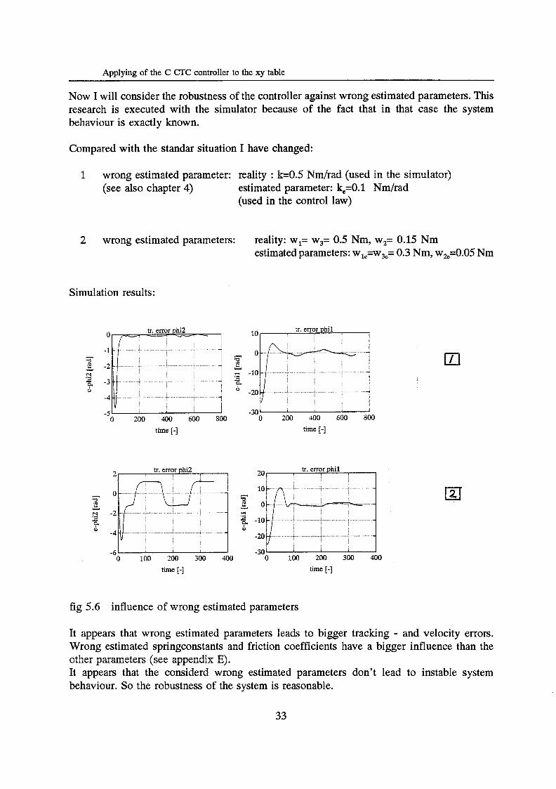
Now I will consider the robustness of the controller against wrong estimated parameters. This research is executed with the simulator because of the fact that in that case the system behaviour is exactly known.
-
-
-4 'v -
-6
Compared with the standar situation I have changed:
1. wrong estimated parameter: reality : k=Q.5 Nm/rad (used in the simulator) (see also chapter 4) estimated parameter: k,=O.l Nm/rad
(used in the control law)
2 wrong estimated parameters: reality: wl= w3= 0.5 Nm, w2= 0.15 Nm estimated parameters: 0.3 Nm, w,=0.05 Nm
Simulation results:
-4w i -5 1 I
O 200 400 600 800 time [-I
7 a
e
Y
2 N
O a
1
Y - .- s -10
-20
-30 O 200 400 600 800
time [-I
tr. error phi1 20 1 5 + -10 1~~ ~
o -20
-30 O 100 200 300 400
time [-I
fig 5.6 influence of wrong estimated parameters
121
It appears that wrong estimated parameters leads to bigger tracking - and velocity errors. Wrong estimated springconstants and friction coefficients have a bigger influence than the other parameters (see appe~dix 8). It appears that the considerd wrong estimated Parameters don't lead to instable system behaviour. So the robustness of the system is reasonable.
33

Applying of the C CTC controller to the xy table
To get an idea of the control prestations, I have made a comparison between the control prestations of a C CTC controller and a CTC controller. Till now the controlling of robots (with or without flexibilities) is in much cases executed by the CTC control strategy. To design a CTC controller the elasticity of the system is neglected. So, the starting point of designing a CTC controller to control the flexible xy table is a model of the xy table without flexibilities. The model of the xy table with a stiff transmission is (see v.d. Molengraft):
7- -2 -
-4 "'
-6
-
-
rn2Cp2+nd2 = us mlipi+nrul = ue
This model is used to design the CTC controller:
li, = m2@ 2 r + ~ d 2 2
u, = ml@ lr+nrull +klei,, (5.9)
I have used above CFC law t~ control the flexible xy table. The simulationresults are:
- desired trajectory A - measure frequence UO.01 H e n += 1 sec. = 100 timesteps - control gain parameters: k,= k2= 0.05, hl= h2= 25
û e Y
cl! c
û E Y
time [-] time [-1
fig 5.7 simulation results CTC controller
If we make a comparison between the control prestations of the C CTC controller (see standard situôtion) and the CFC controller, it appeôrs that the control prestations of the C CTC controller are (much) better. The flexibility of the system plays an important ïole, but
34

Applying of the C CTC controller to the xy table
it appears that this flexibility doesn’t lead to an instable system behaviour (see also appendix
Note: For a system with flexible transmissions controlled by the general CTC law it is not possible to guarantee the stability.
E>.
The mean conclusion of this part of the research is that the C CFC law answers to our desirements. The tracking - and velocity errors converge in all considered cases to zero (to small values). The speed of controlling is reasonable. Further it appers that the robustness of the control system is reasonable, and that the control prestations of the C CTC controller are better than the control prestations of the CTC controller.
35
Controlling of the end-effector
6. CONTROLLING THE END-EFFECTOR
The mean reason of controlling the xy table is that the end-effector will track a certain desired path. To achieve this, the designed C CI'C control routine has to be changed fkom a state control routine (a + g,J to an output control routine ( [x,y] - [xd,yd] ), see also page 12. During this part of the research I have try to find a suitable way to change the C CTC state control routine in a C CI'C output control routine. In this chapter I will show and discuss how the C @TC routine is changed, and I will show and discuss some simulation - and experimental results.
Note: this part of the research has to be considered as trial and error research.
Output control
In order to get reasonable tracking of the desired end-effector path, I have try to find a routine to generate the desired trajectories qza and (Pld on-line. For the on-line generation of the desired trajectories (pa and the obliqueness of the slideway of the xy table (= ~ p i - ( ~ 3 ) is considered. This obliqueness is discounted in the on-line generation. The desired trajectories (pzd and cpld are generated in such a way that the end-effector will track a certain desired path [xd,Yd], no matter how big the value of the obliqueness (~pi'(~3).
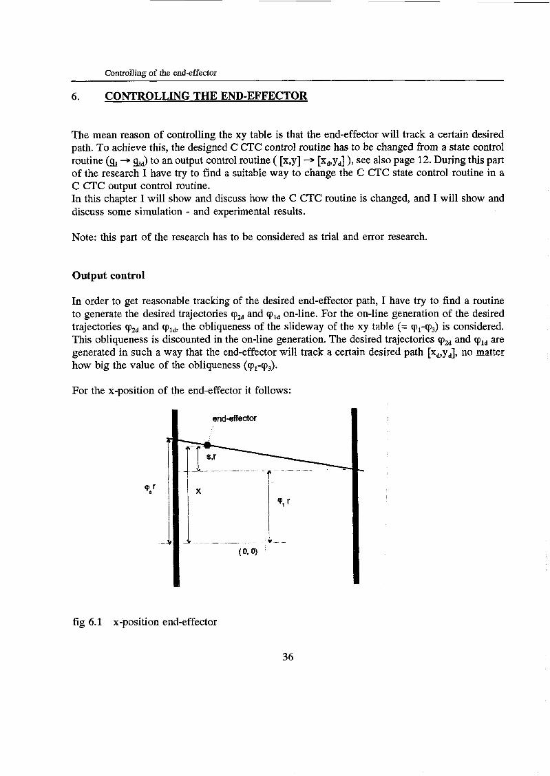
For the x-position of the end-effector it follows:
end-effector
X
I 1
fig 6.1 x-position end-effector
36
Controlling of the end-effector
x = cpPr+sxr (6.1)
See appendix F for s,
The desired path in x-direction of the end-effector is xI. With equatie:: (6.1) it is possible to define an on-line generation routine of the desired trajectory of vi:
On point of time t the routine generates the value of the desired trajectory cpld belonging to point of time t+At. So, on every discret timestep the routine generates the next value of cpld’
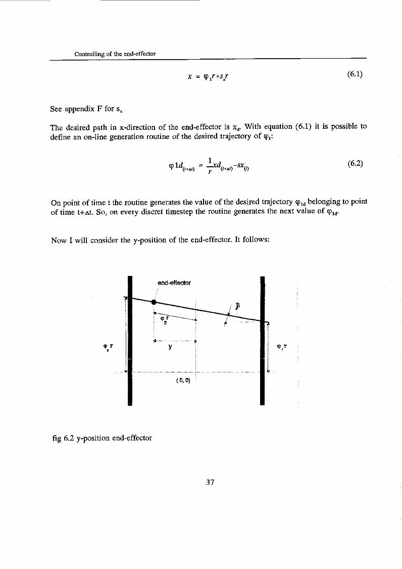
Now I will consider the y-position of the end-effector. It follows:
I end-eff ector I
c----j Y I
fig 6.2 y-position end-effector
37
Controlling of the end-effector
(6.3) y = cp,rcosp
Equation (8.3) can be written in the following form (see appendix F):
Y = cp,r-sy
The desired trajectorie of cp, can be defined as:
Now we have defined an output control routine which is based on the C C ï C strategy. This routine generates with (6.2) and (6.5) on-line the desired trajectories (Pzd and cp1d .
Simulations and experiments
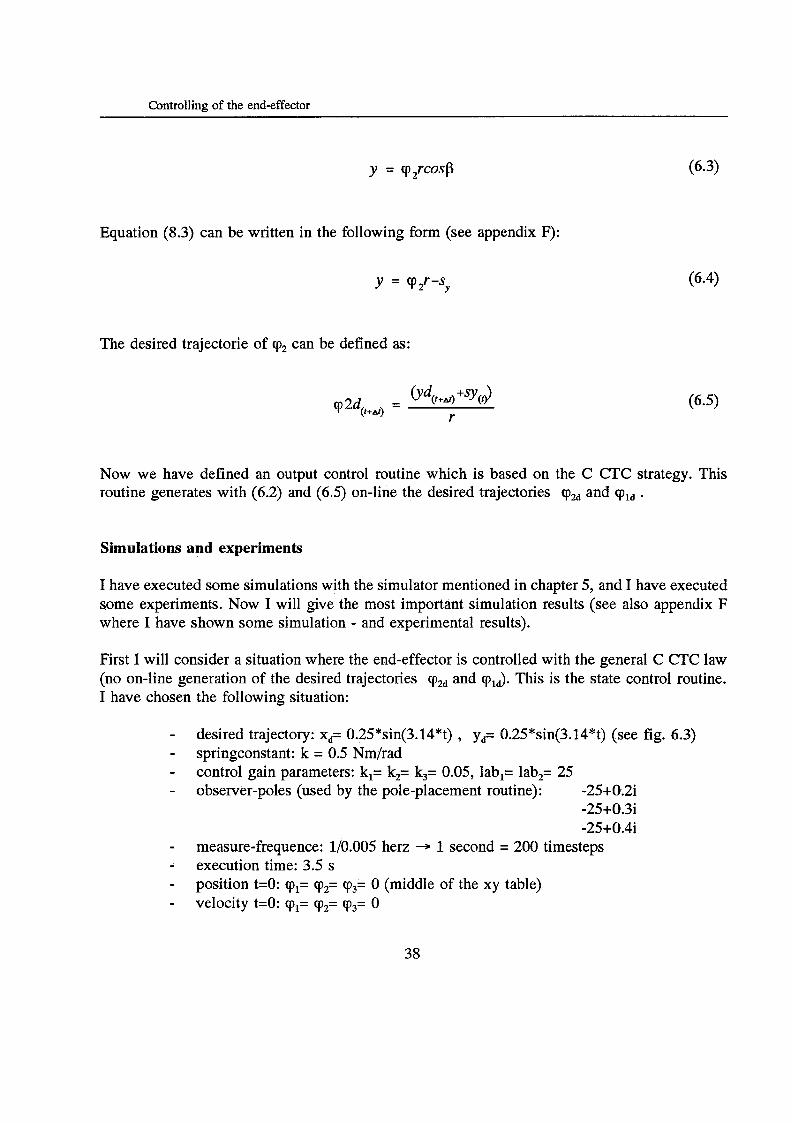
I have executed some simulations with the simulator mentioned in chapter 5, and I have executed some experiments. Now I will give the most important simulation results (see also appendix F where I have shown some simulation - and experimental results).
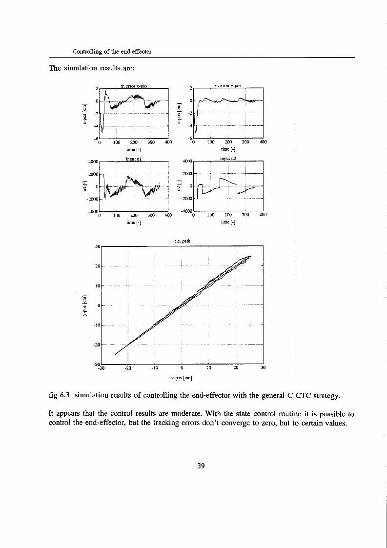
First I will consider a situation where the end-effector is controlled with the general C CTC law (no on-line generation of the desired trajectories (P2d and cp,& This is the state control routine. I have chosen the following situation:
desired trajectory: xd= 0.25*sin(3.14*t) , yd’ 0.25*sin(3.14*t) (see fig. 6.3) springconstant: k = 0.5 Nm/rad control gain parameters: k,= k,= k3= 0.05, lab,= lab,= 25 observer-poles (used by the pole-placement routine): -25+0.21
-25+0.31 -25+0.4i
measure-frequence: l/0.005 herz + 1 second = 200 timesteps execution time: 3.5 s position t=O: cpl= cp2= cp3= O (middle of the xy table) velocity t=O: epi= cp2= cp3= O
38
Controlling of the endeffector
The simulation results are:
tr. error x-pos 1
-6 I I o 100 200 300 400 time [-]
tr.error - s
-2 ~~
-4L -6 O 100 200 300 400
time [-I in utu2
~~~ -2000 O 100 200 300 400
4000
2000
- 0
-2000
-“O 100 200 300 400
- Y
-4000
time [-] time [-I
e.e. oath
fig 6.3 simulation results of controlling the end-effector with the general C CTC strategy.
It appears that the control results are moderate. With the state control routine it is possible to control the end-effector, but the tracking errors don’t converge to zero, but to certain values.
39
Controlling of the endeffector
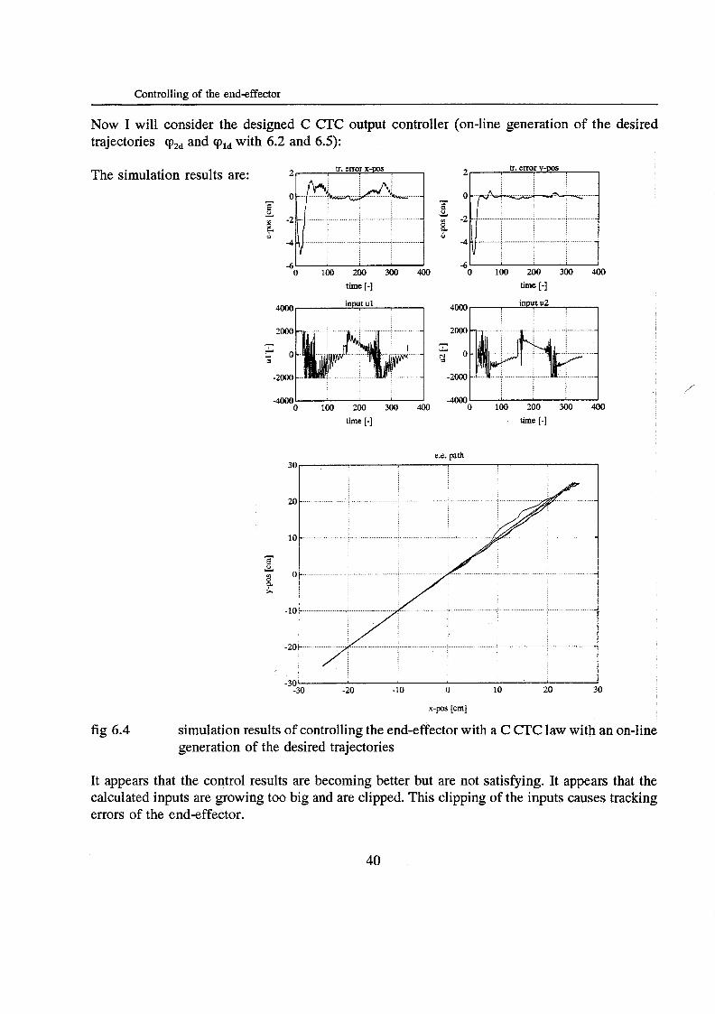
Now I will consider the designed C CTC output controller (on-line generation of the desired trajectories cpZd and cpid with 6.2 and 6.5):
The simulation results are:
o 100 200 300 400 o 100 200 300 400 time [-] time [-]
o 100 200 300 400 o 100 200 300 400 time [-] time [-I
e.e. path
x
fig 6.4
x-pos [cm]
simulation results of controlling the end-effector with a C CTC law with an on-line generation of the desired trajectories
/
It appears that the control results are becoming better but are not satisfying. It appears that the calculated inputs are growing too big and are clipped. This clipping of the inputs causes tracking errors of the end-effector.
48
Controlling of the end-effector
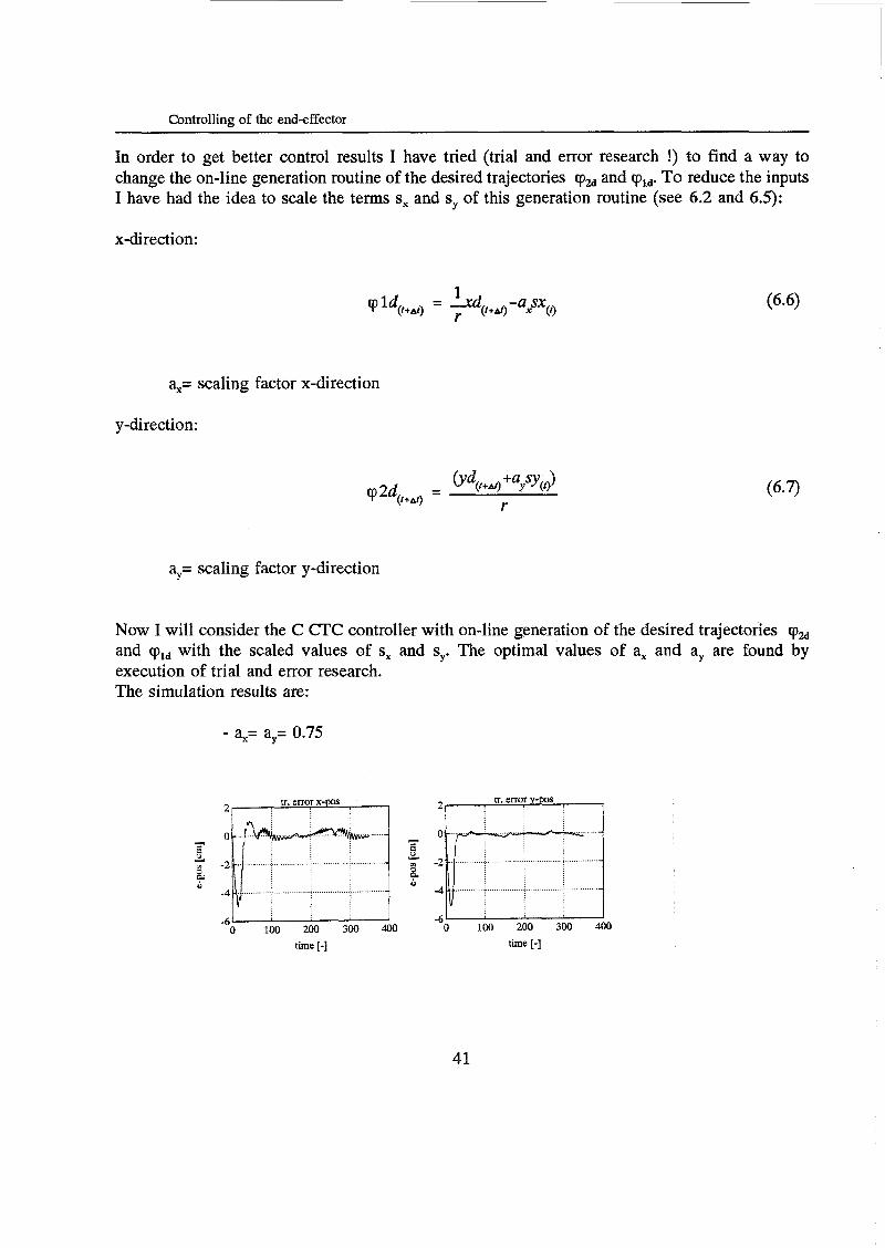
In order to get better control results I have tried (trial and error research !) to find a way to change the on-line generation routine of the desired trajectories and vid. To reduce the inputs I have had the idea to scale the terms s, and sy of this generation routine (see 6.2 and 6.5):
x-direction:
ax= scaling factor x-direction
y -direction:
ay= scaling factor y-direction
Now I will consider the C CTC controller with on-line generation of the desired trajectories cpZd and cpid with the scaled values of s, and sy. The optimal values of a, and ay are found by execution of trial and error research. The simulation results are:
- a,= ay= 0.75
tr. error Y-POS 2, I 2, I tr. error x-pos
time [-3 time [-I
41

Controlling of the endeffector I 1 . .._ . ._ . . . ~ ........._.__ ~ ......... _._,.._...__.......
fig 6.5
I -30 -20 -10 O LO ZO 30
“pos [cml
-301
simulation results of controlling the end-effector with a C CïC law with an on-line generation of the desired trajectories. Now s, and sy are scaled.
It appears that this on-line generation routine leads to the best control results.
The mean conclusion of this part of the research is that the by trial and error research designed output control routine leads to reasonable control results. In order to get better results this part of the research has to be executed on a more fundamental way.
42

Conclusions and recommendations
7. CONCLUSIONS AND RECOMMENDATIONS
Conlusions
For the controlling of the xy table with one flexible transmission it is possible to design a control law iwk_Lch is based on the C CTC strategy. The goal of applying this C CTC Controller is to track the desired trajectory qld= [qad 9p1JT and its time derivative. This is a state control routine.
It can be proved that applying of the C CTC law to control the flexible xy table leads to a stable system behaviour.
The simulation results which are related with the theoretical situation confirm with the expectations, and give a good picture of the properties of the C CTC controller.
From the simulations it appears that there will be a reasonable change that the C CTC controller applied in a practical situation will answer to our desirements ( robust system behaviour, small tracking errors).
The implementation of the C CTC law and an observer algorithm (for the reconstruction of the angular velocities) in the control system of the xy table is succeeded.
For the testing of designed control laws or system configurations and for the execution of a part of the research I have designed a simulator. The simulator fits the reality on a close way.
The new software designed by Jos Banens meant for the total organisation of executing experiments and simulations, is easy and pleasant to use.
The experimental results and accessory simulation results answers to our desirements. The tracking - and velocity errors converge to zero (to small values). The control speed is reasonable. Further it appears that the robustness of the control system is reasonable and that the control results are better that the control results of the general CTC law.
For the controlling of the end-effector I have designed (by trial and error) a C CTC output control routine. This routine generates on-line the desired trajectories of qi and cp2 . The results of this control method are reasonable.
43
part 2
COMPOSITE COMPUTED TORQUE CONTROL OF THE xi! TABLE WITH AN ELASTIC MOTOR TRANSMISSION
theoretical analysis, simulations and experiments
by: Gen Brevoord
Professor: prof. dr. ir. J.J. Kok Coach: ir. I.M.M. Lammerts
WFW, Control and identification of Mechanical systems Department of Mechanical Engineering, Eindhoven University of Technology.
Report no.: 92.054
Appendices
APPENDICES:
A:
B:
C:
D:
E:
F:
G:
The model of the xy table
Simulation results of some theoretical situations of the first part of the research.
Simulation results of some practical situations of the first part of the research.
Observer algorithm
Simulation - and experimental results of the second part of the research
Output control
References

The model of the xy table
APPENDIX A: THE MODEL OF THE X Y TABLE
In this appendix I will give a detailed desricption of the model of the xy table ( see v.d. Molengraft, 1989).
The model of the xy table:
r
J2 w2 4 X I
fig a l model of the xy table
The equations of motion of the xy table can be written as:
(Al.l)
A.1
The model of the xy table
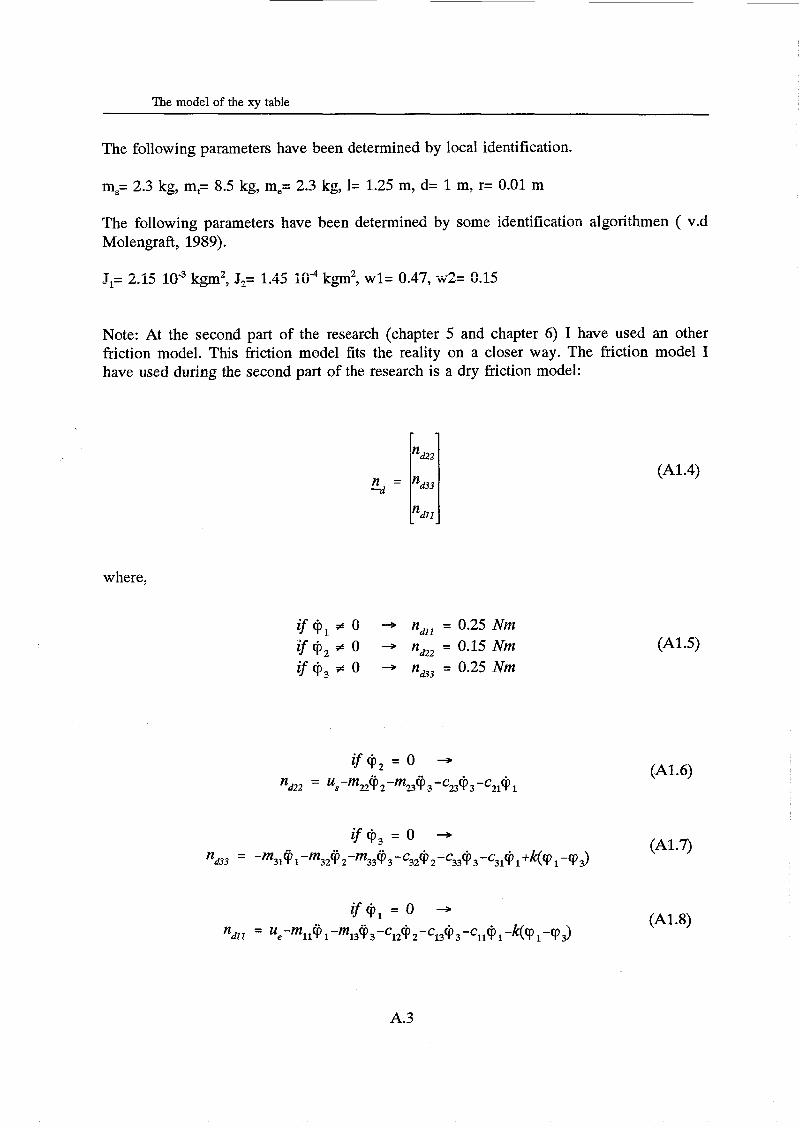
The following parameters have been determined by local identification.
m,= 2.3 kg, mt= 8.5 kg, me= 2.3 kg, 1= 1.25 m, d= 1 m, r= 0.01 m
The following parameters have been determined by some idemtification algorithmen ( v.d Molengraft, 1989).
I,= 2.15 kgm2, J2= 1.45 íG4 k p 2 , wl- 0.47, w2= 0.15
Note: At the second part of the research (chapter 5 and chapter 6) I have used an other friction model. This friction model fits the reality on a closer way. The friction model I have used during the second part of the research is a dry friction model:
where,
i f@, # O -* Itdll = 0.25 Nm if@, # O + nd22 = 0.15 Nm if@, # O -* Itd3 = 0.25 Arm
(A1.4)
(A1.5)
(A1.6)
(A1.8)
A.3
B: Simulation results of some theoretical situations of the first part of the research
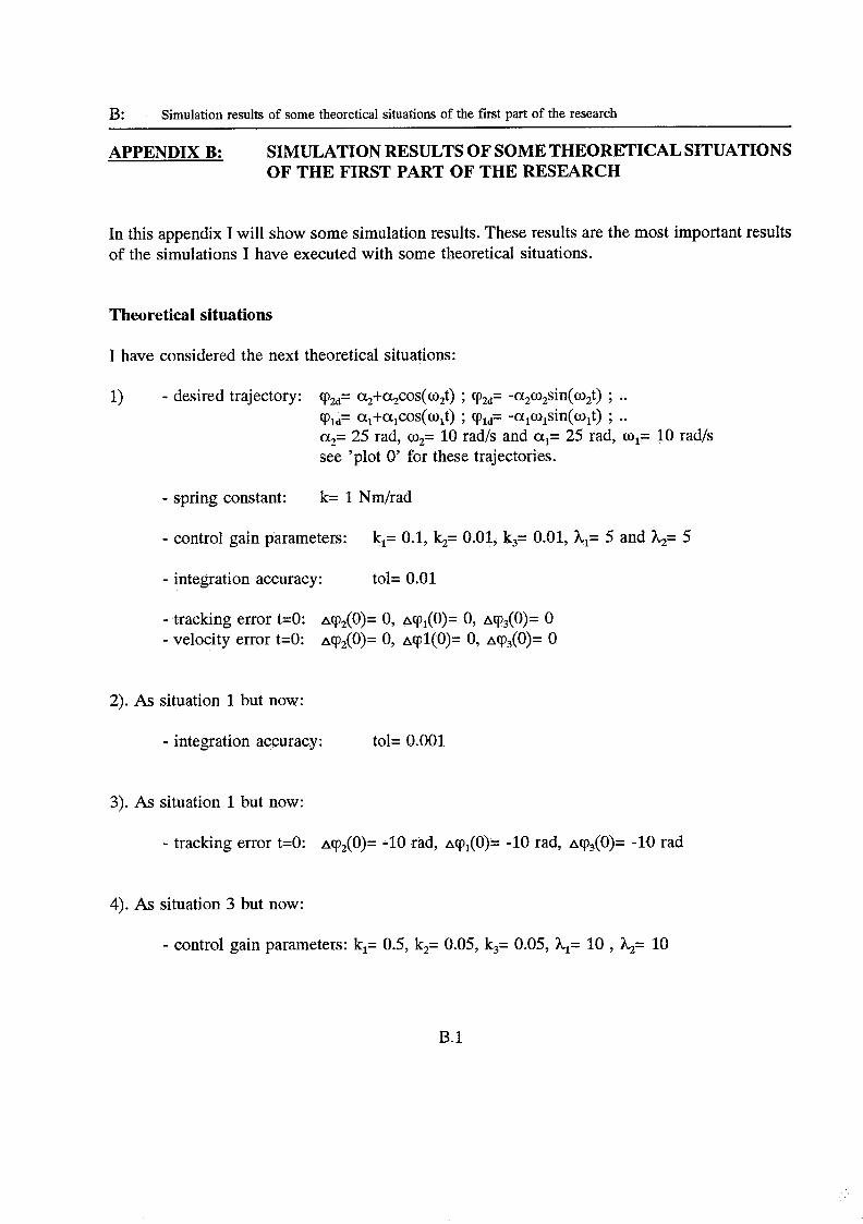
APPENDIX B: SIMULATION RESULTS OF SOME THEORETICAL SITUATIONS OF THE FIRST PART OF THE RESEARCH
In this appendix I will show some simulation results, These results are the most important results of the simulations I have executed with some theoretical situations.
Theoretical situations
I have considered the next theoretical situations:
1) - desired trajectory: T2d= c~~+a~cos (w~t ) ; 02d= -a2m2sin(w2t) ; .. qld= al+cL1cos(wlt) ; cpld= -alm,sin(wlt) ; .. q= 25 rad, co2= 10 radls and al= 25 rad, m1= 10 rad/s see ’plot O’ for these trajectories.
- spring constant: k= 1 Nm/rad
- control gain parameters: k,= 0.1, k2= 0.01, k3= 0.01, h,= 5 and A,= 5
- integration accuracy: tol= 0.01
- tracking error t=O: A(P~(O)= O, ~cp,(O)= O, ~ c p ~ ( O ) = O - velocity error t=O: arp2(0)= O, ~ r p l ( O ) = O, ~ c p ~ ( O ) = O
2). As situation 1 but now:
- integration accuracy: tol= 0.001
3). As situation 1 but now:
- tracking error t=O: ~cp,(O)= -10 rad, ~cp,(O)= -10 rad, ~ c p ~ ( O ) = -10 rad
4). As situation 3 but now:
- control gain parameters: k,= 0.5, k2= 0.05, k3= 0.05, hl= 10 , &= 10
B. 1
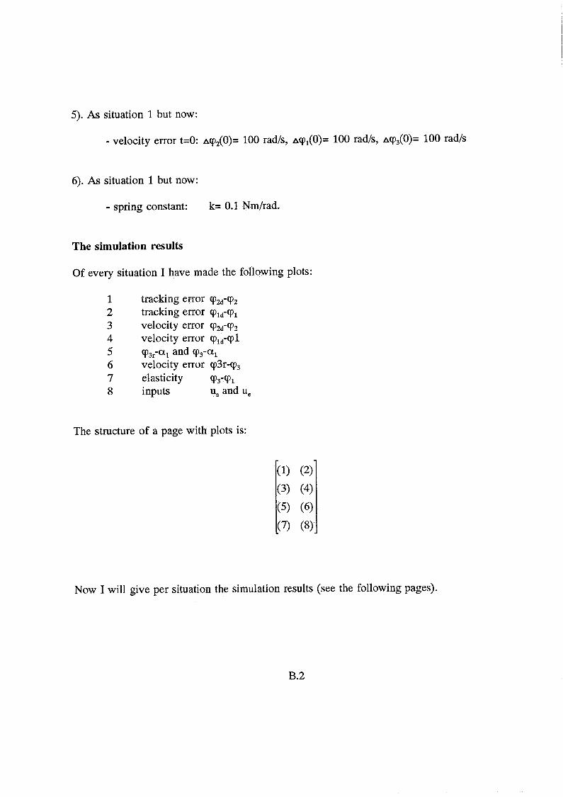
5). As situation 1 but now:
- velocity error t=O: A(P*(O)= 100 rad/s, ~cp,(O)= 100 rad/s, acp3(0)= 100 rad/s
6). &As situation 1 but now:
- spring constant: k= 0.1 Nm/rad.
The simulation results
Of every situation I have made the following plots:
1 tracking error cpzd-cp,
2 tracking error cpld-ql
3 velocity error cpzd-cp,
4 velocity enor qid-q1
6 velocity error cp3r-cp3
8 inputs u, and u,
5 cp3r-% and 9 3 %
7 elasticity V3-9 1
The structure of a page with plots is:
Now I will give per situation the simulation results (see the following pages).
B.2

Simulation results of some theoretical situations
Desired trajectorie: plot O
I
- -5 E I Y
.- N c a
time [s] time [SI I
400
- 200 r 3,
O 3, * -200
ï Y
.- r I
I
-400 O 1 2 3 O 1 2 3
time[s] I

Simulation results of some theoretical situations
situation 1
20
- 10 ___._.,'$ ........... ........................... i ................... A- , < I ;; I - * i ; -\ , , I . , 1 '
, ( * : , , I : I , I , , a # ( I ' < ' 1 0- I < , I I j < I , . I : '
I ' , I L I , ' , , ; : : ; ' $ ; , I
, I : ::
*, ... I < , < , I E 5
2 , I cc
z ............ rn - 10 2.. ..... ,:!?y ......:.... :;. >;.;...........i; .
I -
trackine error phi2 0.02
v
N .- =y -3.91 o
.....................
O I 2 3 -0.03
time [SI tracking error dphi2
1
tracking error phi1 0.04
0
. . . . . . . . . . . . .
O 1 2 3
time [SI tracking error dphil
-0.04
I
1 O 1 2 3 -1 '
time [s]
I O 1 2 3
time [SI -1 '
desired trajectory: plot O, k= 1 Nm/rad, integration accuracy: tol= 0.01, tracking error t=O: acpZ(O)= O, ~cp , (O)= O, acp,(O)= 0 velocity error t=O: ~ c p ~ ( O ) = O, ~ c p l ( O ) = O, ~cp , (O)= O
control par.: k,= 0.1, k,= 0.01, k,= 0.01, Al= 5 and &= 5
Simulation results of some theoretical situations
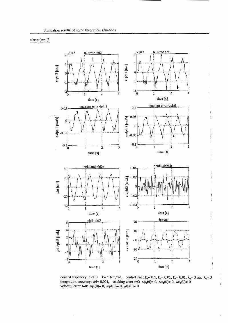
situation 2
xlO-3 tr. error phi2 I I
1 c
-2 .- N O L, Y
c : -1
-2 1 2 3 O time [s]
0.05
O i- - c\1 c .- a -0.05
O 1 2 3 -0.1
time [s]
phi3 and phi3r 40 1
1 I 3 -40 i
O 1 2
time [s]
phil-phi3
i
time fs]
time [s]
o. 1 tracking error dphil
1
2 3 -0.1 L O 1
time [SI
dphi3-dphi3r 0.04
0.02 3 i- u z o Y -0.02
c c
I O 1 2 3 -0.04'
time [s]
inputs 20
I
O 1 2 3 -20'
time [s]
desired trajectory: plot O, k= 1 Nm/rad, integration accuracy: tol= O.OOI, tracking error t=O ~ c p , ( O ) = O, ~cp , (O)= O, ~cp , (O)= O velocity error too: ~ c p , ( O ) = 0, ~cpí(û)= O, A~,(O)= O
control par.: k,= 0.1, k,= 0.01, k3= 0.01, hl= 5 and &= 5
Simulation results of some theoretical situations
- .. . . .i. ....................... ............... ._
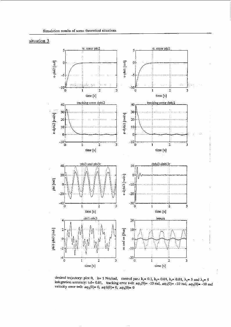
situation 3
0 -20
5 tr. error hi2
.- Y N c ü L. :.'i .- Y s 4 i: 0
-5 -5
-10 -10 O 1 2 3 O 1 2 3
time [SI time [SI
............... j. ............... ....i ...............
1
L; Y
R
N c c .-
2
I O - . . ; >.... 2 <... . . . . . . . . . . . . . . . . . . . . . . . . . . . . . I ._ ....... ........... - I > ) ; ; ,,?, ;e', , #I ',\ ; ',
- 4 2
- 2
i u 4
c 2
-1 o O 1 2 3
time [SI -101 I
O 1 2 3 time [SI
time [SI ~~
time [SI
desired trajectory: plot O, k= 1 Nm/rad, control par.: kl= 0.1, k2= 0.01, k3= 0.01, hl= 5 and &= 5 integration accuracy: tol= 0.01, tracking error t=O ~cp , (O)= -10 rad, ~ c p , ( O ) = -10 rad, ~ c p , ( O ) = -10 rad velocity error t=O ~ c p , ( O ) = O, ~ r p l ( O ) = O, ~ c p ~ ( O ) = O
Simulation results of some theoretical situations
5
-
1
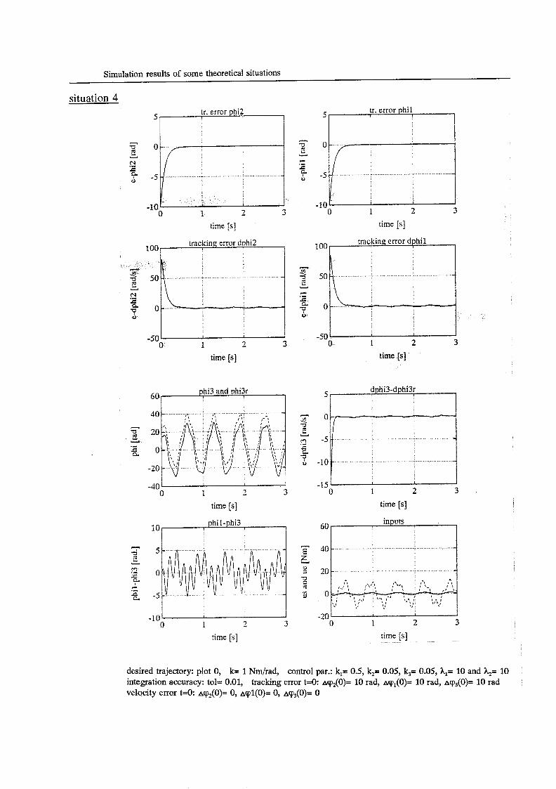
situation 4
5
o
-5 -.
c - -
-10
-15
-
I I
I 7 n L-
60
40 ................ ~ ...................... f ......................
20 _. ............................ ..:
# I ,.; ,.,'T, I'.., p<- , I s : ; , I , , l \ . . . . . . . . 0- , , ',., I t - ,
,. , t \ , 1 I I ,I'
'.' :: I>
t I 3 -xu
O 1 2 time [SI
tracking error dphi2 1001 1
I I 3 -50
O 1 2 time [s]
phi3 and phi3r 60 1
I 3
-40 O 1 2
time [SI Dhi I-ohi3 i 0 -1
- 5 f z
2 O
3 3
n -5 3
3 -10
O 1 2 time [SI
time [SI
-30 ' I o 1 2 3
time [SI ~
desired trajectory: plot O, k= 1 Nm/rad, integration accuracy: tol= 0.01, tracking error t=O ~cp,(O)= 10 rad, ~cp,(O)= 10 rad, AT@)= 10 rad velocity error t=O ACP,(O)= O, ~rp í (O)= O, ~cp,(O)= O
control par.: kl= 0.5, k2= 0.05, k3= 0.05, hl= 10 and %= 10
Simulation results of some theoretical situations
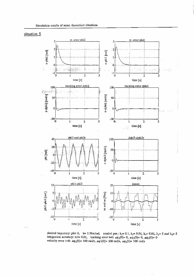
situation 5 3 , tr. error phi2
2 ..................................................
2
?-
.- Y z k : N 1 .................. .......................................... 1 c
e, o ........... 5--1
-1 - O 1 2 3
time [SI
-50 O L 2 3
time [SI
O 1 2 3 time [SI
tracking error dphil 100, I
time [SI
phi3 and phi3r 40 1 1 O0
0
50 e 20
O 7% Y
rn c .-
a = o -20 u
-40 I O 1 2 3
time [SI phii-pni3 10
-50 ' I O 1 2 3
time [SI inputs 20 i
-20 ' f I I O 1 2 3
time Es]
10 O 1 2 3
time [s]
desired trajectory: plot O, integration accuracy: tol= 0.01, tracking error t=O: ~cp,(O)= O, ~cp~(o)= O, ACP,(~)= 0 velocity error t=O: ~cp,(O)= 100 rad/s, ~ r p l ( O ) = 100 rad/% ~rp,(O)= 100 rad/s
k= 1 Nm/rad, control par.: k,= 0.1, k,= 0.01, k3= 0.01, hl= 5 and &= 5
Simulation results of some theoretical situations
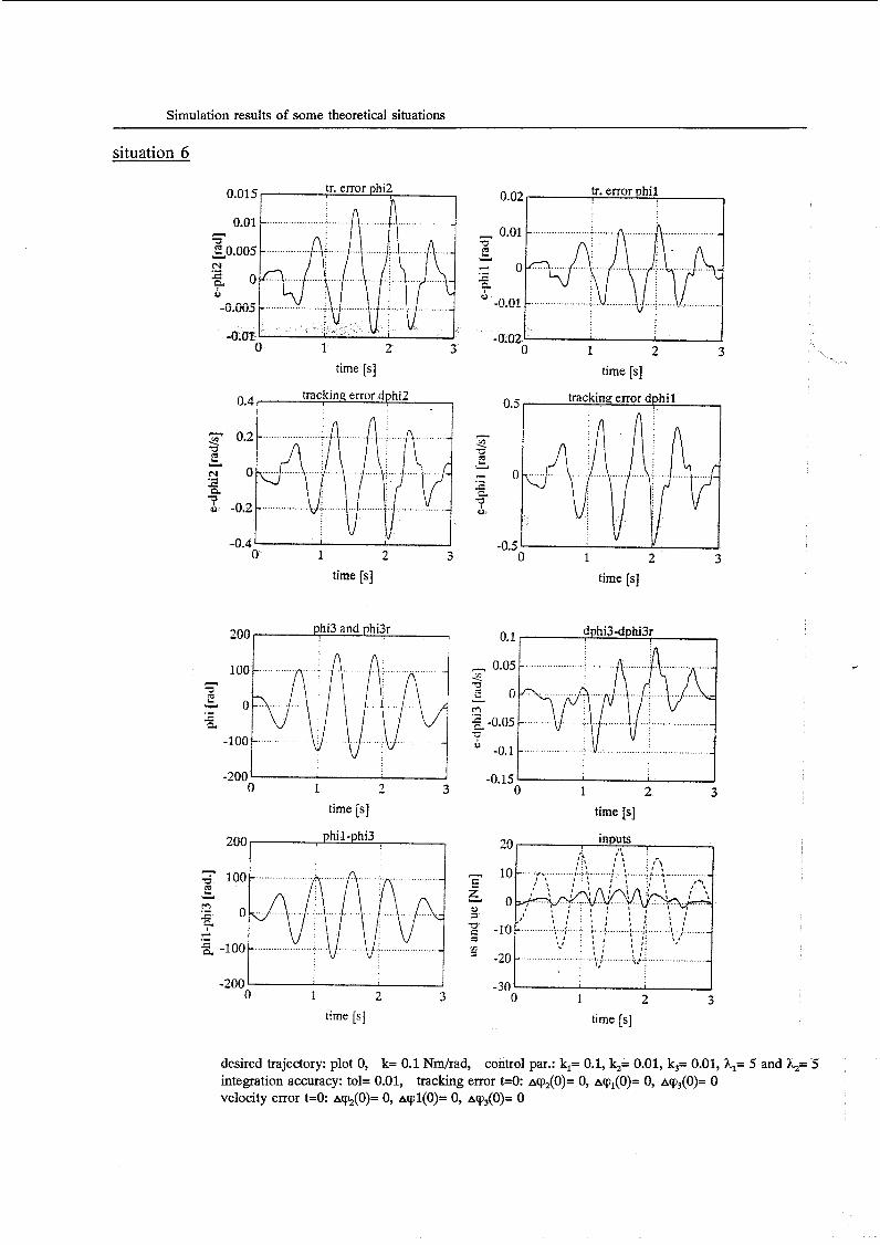
situation 6
tr. error phi2 0.015 1 n 1
O 1 2 3
tr. error phi1 0.02 f 1
-0.02 O 1 2 3
time [SI time [SI trackine: error dphil
0.4 I I 0.5 I I
tracking error dphi2
- 4 0.2 T ii Y
O - o - c - c I Q -0.2 o
-0.4 -0.5 1 2 3 O 1 2 3 O
time [SI time [SI
dphi3-dphi3r o. 1
- 0.05 -
-
-0.15 O 1 2 3
time [SI time [s]
200
3 100
c o $"
a -100
m m iLi u
.-
4 .-
-200 3 3 o 1 2 3 O 1
time [SI time [SI
desired trajectory: plot O, integration accuracy: tol= 0.01, tracking error t=O: ~ c p , ( O ) = O, ~cp,(O)= O, ~rp,(O)= O velocity error t=O: ~cp,(O)= O, ~ c p l ( O ) = O, ~cp,(O)= O
k= 0.1 Nm/rad, control par.: kl= 0.1, k,= 0.01, k,= 0.01, hl= 5 and &,= 5

c: Simulation results of some practical situations of the first part of the research
APPENDIX C: SIMULATION RESULTS OF SOME PRACTICAL SITUATIONS OF THE FIRST PART OF THE RESEARCH
In this appendix I will show and discuss some simulation results. These results are the most important results of the simulations I have executed with some practical situations.
Practical situations
I have considered the next practical situations:
1) - desired trajectory: qZd= q+cr,cos(m,t), ... qld= a1+a1cos(6q), ... cx2= 25 rad, m2= 1 rad/§ and a,= 25 rad, ml= 1 radls
- spring constant:
- control gain parameters:
k= 1 Nm/rad
k,= 0.5, k2= 0.05, k3= 0.05, hl= 10 and A,= 10
- integration accuracy: can not be chosen
- discretization: Atr= 0.001 S , Att,= 0.005 S (Atm= 0.006 S )
- particularies: none ( no start errors, no wrong parameter estimations, no unmodelled dynamics, etc.)
2) As situation 1 but now:
- m2= 10 rad/s, ml= 10 radh.
3) As situation 2 but now:
- discretization: At,= 0.002 S , Att,= 0.008 s (Atm= 0.01 s)
4) As situation 2 but now:
- discretization: At,= 0.005 S , Att,= 0.005 S (Atm= 0.01 S )
c. 1
c: Simulation results of some practical situations of the first part of the research
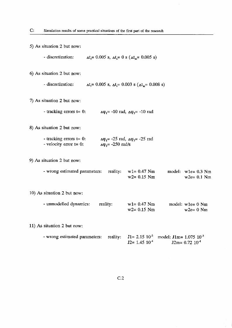
5) As situation 2 but now:
- discretization: Att,= 0.005 S, Att,= 0 S (At,= 0.005 S )
6) As situation 2 but now:
- discretization: Att,= 0.005 S, Ats= 0.003 S (At,= 0.008 S)
7) As situation 2 but now:
- tracking errors t= O: A(P~= -10 rad, A(P~= -10 rad
8) As situation 2 but now:
- tracking errors t= O: - velocity error t= O:
AT;= -25 rad, ~ p ~ = -25 rad hcp2= -250 rad/s
9) As situation 2 but now:
- wrong estimated parameters: reality: w l= 0.47 Nm model: wle= 0.3 Nm w2e= 0.1 Nm w2= 0.15 Nm
10) As situation 2 but now:
- unmodelled dynamics: reality: w l= 0.47 Nm model: wle= O Nm w2e= O Nm w2= 0.15 Nm
11) As situation 2 but now:
- wrong estimated parameters: reality: J1= 2.15 lo5 model: Jlm= 1.075 10” J2= 1.45 lo4 J2m= 0.72 lo4
c: Simulation results of some practical situations of the first part of the research
12) As situation 2 but now:
- unmodelled dynamics: reality: k= 1 Nmhad model: ke= 0.7 Nm/rad
13) As situation 2 but now:
- unmodelled dynamics: of situation 9:11 and 12.
14) As situation 3 but now:
- spring constant: k= 0.1 Nm/rad
15) As situation 3 but now:
- measure errors: - angular position + white noise vp= %rand(t) + %= 0.1 - angular velocity white noise v,= wand(t) + %= 1
note: rand(t)= white noise, between -1 and 1.
Simulation results
I have made the same plots of every situation as of the theoretical situation ( see appendix B). The structure of a page with plots is the same as given in apendix B. Now I will give per situation the simulation results (see the following pages).
c .3
Simulation results of some practical situations
0 -
-0.2
-0.4
-0.6
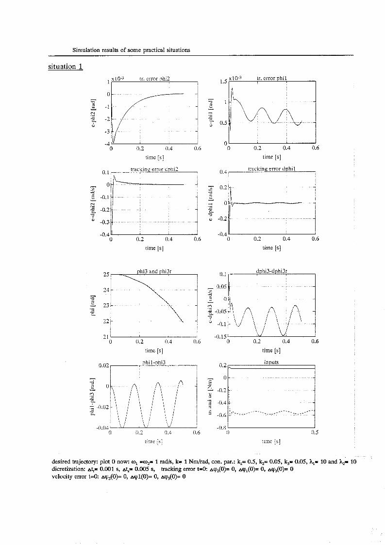
situation 1
. . . . . . . . . . -
. .. .- t
t. ::-------- -
. . . . . . - _ - - - - - - _ _ - _ - - - _ _ -.___-- _- - -_
x10-3 tr. error phi2 l i I
- 3 ï u .- c - c
7
O 0.2 0.4 0. 6
time [SI trackint! error dphi2 0.1 1 1
time [s]
trackin,g error dph i l 0.4
0.2 -
-0.2 -
-0.4
-
o 0.2 0.4 0.6
i -0.4 " I o 0.2 0.4 0.6
time [s] time [SI
phi3 and phi3r 25
24 1 23 c 21 ' J
0 0.2 0.4 0.6
dphi3-dphi3r 0. 1
time [SI time [SI innuts û.2 b-1
-03 ' J o 0.5 time [SI
desired trajectory: plot O now: o1 =o2= 1 rad/s, k= 1 Nm/rad, con. par.: kl= 0.5, k,= 0.05, k3= 0.05, &= 10 and &= 10 dicretization: A$= 0.001 s, at,= 0.005 s, tracking error t=O: acp,(O)= O, acp,(O)= O, acp,(O)= O velocity error t=O ~cp,(O)= O, ~ c p l ( O ) = O, ~ c p , ( O ) = O
Simulation results of some practical situations
situation 2
tr. error phi2 o. 1 1 tr. error phi1 o. 1
0.05 .....................
.....................
..... ..................... -0.05 -0.05 .....................
-0.1 I O 1 2 3
time [SI tracking error dphi2 4 , , I
............... ...:. ................................
I I
-6l I O 1 2 3
time [s]
phi3 and phi3r 40
20 - 3
Y o .- c a -20
-40 - O 1 2 3
time [SI 5 , ohil-phi3
1
O 1 2 3 time [SI
m .-
-0.1 - O 1 2 3
time [SI
.....................
O 1 2 3 time [s]
.................
P)
3 E .13
a
9
-20 - O 1 2 3
time [s]
time [SI
desired trajectory: plot O, k= 1 Nm/rad, control par.: kl= 0.5, k,= 0.05, k3= 0.05, hl= 10 and &= 10 dicretization: at,= 0.001 s, at,= 0.005 s, tracking error t=O: acpz(0)= O, acp,(O)= O, acp,(O)= O velocity error t=O: acpZ(O)= O, ~ c p l ( O ) = O, ~cp,(O)= O
Simulation results of some practical situations
situation 3 tr. error phi2 0.2
-0.2 O 0.5 1 1.5 2
time [SI tracking error dphi2 10
time [SI tracking error dphil 10, 1
U
-10 O 0.5 1 1.5 2
time [SI
phi3 and phi3r 40
-10 i I I
O 0.5 1 1.5 2 time [s]
dphi3-dphi3r 40,
-40' 1 O 0.5 1 1.5 2
time Is]
-40 O 0.5 1 1.5 2
time [ s ]
O 0.5 1 1.5 2 time [ s ]
-20 I 3 I I O 0.5 1 1.5 2
time [s]
desired trajectory: plot O, k= 1 Nm/rad, control par.: k,= 0.5, k2= 0.05, k3= 0.05, hl= 10 and &= 10 dicretization: at,= 0.002 s, at,= O.OO8 s, tracking error t=O: acp,(O)= O, AC~,(O)= O, arp3(0)= O velocity error t=O ~cp,(O)= O, ~ c p l ( O ) = O, a~p,(O)= O

Simulation results of some practical situations
50
Y -
c i 3 I
i l -40 -50 - '
situation 4
tr. error phi3 0.3
- 0.1
.- N O
- 3 i L
c
-0.2 -0.4 0 0.2 0.4 0. 6 o 0.2 0. 4 0.6
time [SI time [SI
-10 trackinc error ciplii2 10
0.4 0. 6 O 0.2 0.4 0.6
.- N O
-10 0 0.2
time [SI time [SI
desired trajectory: plot O, k= 1 Nm/rad, control par.: kl= 0.5, k,= 0.05, k3= 0.05, hl= 10 and %= Iû dicretization: at,= 0.005 s, at,= 0.005 s, tracking error t=O: acp,(O)= O, acp,(O)= O, acp3(0)= O velocity error t=O: ~ c p , ( O ) = O, ~ c p í ( O ) = O, ~ c p , ( O ) = O
Simulation results of some practical situations
situation 5
tr. error phi2 0.2 tr. error phi1
0.2
I
2 3 -0.2 ' O 1
time [SI tracking error dphi2
i
I 1
2 3 -0.2 ' O 1
time [SI tracking error dphil 20 1
I O 1 2 3
time [SI -10'
phi3 and phi3r 40 r 1
20 3 v o .- c a
-20
O 1 2 3 -40
time [SI
P)
u O 1 2 3
time [SI -20
O 1 2 3 -60
time [SI
10
n 3 Y E 5 (cl
c .- I i 1 0 c a
O 1 2 3 -5
time [SI time [SI
desired trajectory: plot O, k= 1 Nm/rad, control par.: k,= 0.5, k,= 0.05, k,= 0.05, hl= 10 and &= 10 dicretization: at,= 0.05 s, at,= 0 s, tracking error t=O: ~cp, (O)= O, arp,(O)= O, ~cp,(O)= O velocity error t=ík ~cp,(o)= o, acpí(û)= O, ~ c p , ( O ) = O
Simulation results of some Dractia1 situations
5 40
- 20 E 7 m F
z Y o 3, 3 -20
-5 -40
L Y
.- 2 0 ;I d .- c a
situation 6
tr. error phi2 0.2 I I
_ <.......,..... ~~ .......... .- ...... - ................ ~ ....,. I a , $ : i, : : : I : > , , I 1 I:( ( 1 I ,;.:::::::;:'
- .:.. . ..... . . . . .. . . .... . .......... ;. .d. ... ... ..: .... " .......... -
, r i & : ~ ,, ; ; : : : : ' ( I 4 :
I , ,,,,, y : : : : : :: ': . I :<%,,#" Y , I > ~ I ' c *
1 , 1 1 * 1 1, I I IO * v * 1 :;, t I * :; :; :: J . . c t ;
-0.2' I O 0.5 1
time [SI tracking error dphi2 10, i
tr. error phi1 0.4 1
-0.4 I I O 0.5 1
time [SI tracking error dphil 40, 1
20 E 4 0
c1 s
F -20
Y
.- c p.
-10' I O 0.5 1
time [SI O 0.5 1
time [SI
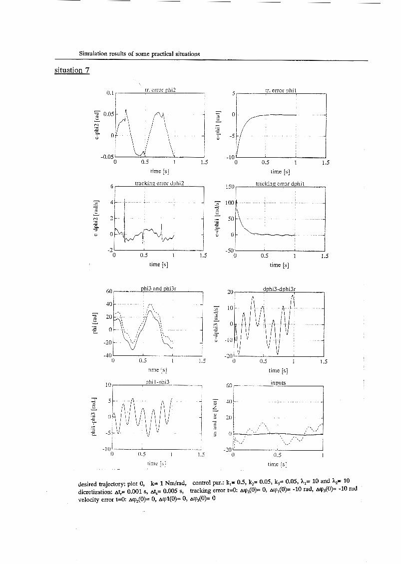
Simulation results of some practical situations
i
situation 7
-
-
-
!
-40 ' I 0 0.5 1 I .5
time [SI phi 1-phi3
- 1 0 ' o 0.5 1 1.5
tinir [b]
-30 1' I o 0.5 1
linie [s]
desired trajectory: plot O, k= 1 Nm/rad, control par.: kl= 0.5, k,= 0.05, k3= 0.05, hl= 10 and &= 10 dicretization: A<= 0.001 s, at,= 0.005 s, tracking error t=O: acp,(O)= o, A ~ ~ ( O ) = -10 rad, acp,(O)= -10 rad velocity error t=O: ~cp, (O)= O, ~ c p l ( O ) = O, acp3(0)= O
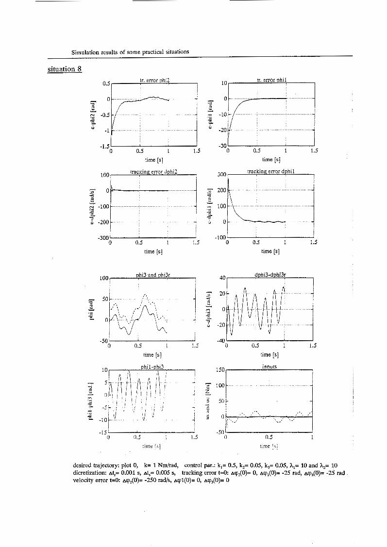
Simulation results of some practical situations
10-
-
-
-
situation 8
1 O0
c( c O E 3 e CI -100- Y
.- - c c 5 -200-
-300
tr. error phi2 0.5
-
-
-
-0.5
-1.5 O 0.5 1 1.5
-1.5' 1 O 0.5 1 1.5
ohil-nhi3
l i
-15: 0 0.5 I 1.5
-501 1 0 0.5 1
desired trajectory: plot O, dicretization: At,= 0.ûûí s, At,= û.ûû5 s, velocity error t=O: ~ c p , ( O ) = -250 rad/s, ~ c p l ( O ) = O, acp,(O)= O
k= 1 Nm/rad, control par.: kl= 0.5, k,= 0.05, k,= 0.05, hl= 10 and &= 10 tracking error t=û: AcpZ(0)= 0, Acpl(0)= -25 rad, Acp,(O)= -25 rad
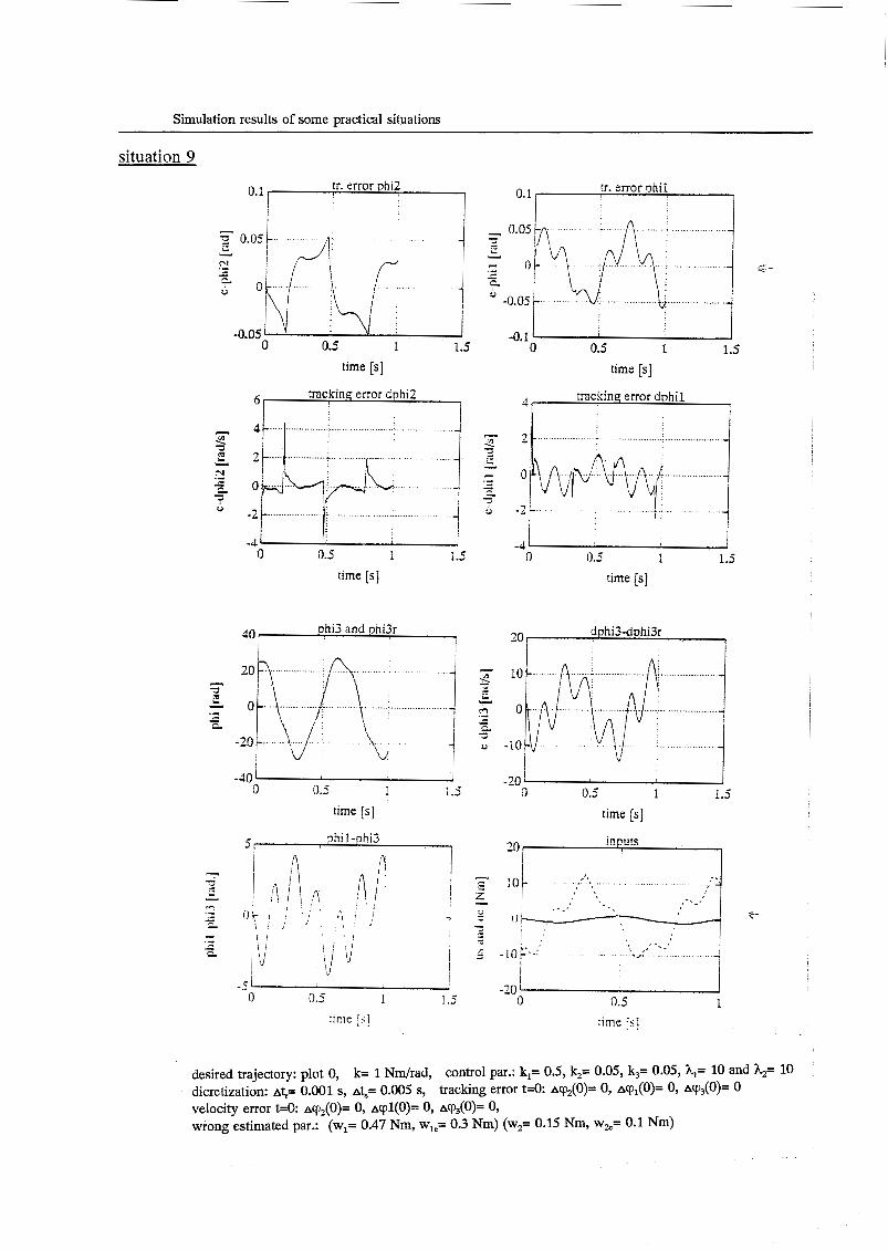
Simulation results of some practical situations
situation 9
-0.05 O 0.5 1 1.5
time [SI tncking error dphi2
1
O 0.5 1 1.5
time [s]
J
o. 1
0.05
o
-0.05
-0.1 O 0.5 1 1.5
time [s]
tricking error dphi l 4,
o+JLPvvy .i -2 -
-4. n 0.5 1 1.5
time [SI 0 0.5 1 1.5
time [SI
G
desired trajectory: plot O, k= 1 Nm/rad, control par.: k,= 0.5, k,= 0.05, Ir,= 0.05, hl= 10 and &= 10 dicretization: aq= 0.001 s, at,= 0.005 s, tracking error t=O. acp,(O)= O, acp,(O)= O, acp,(O)= O velocity erroï t=0: ~qp, (O)= O, ~qpl(O)= O, ~cp, (O)= O, wrong estimated par.: (wl= 0.47 Nm, wie= 0.3 Nm) (wz= 0.15 Nm, wk= 0.1 Nm)
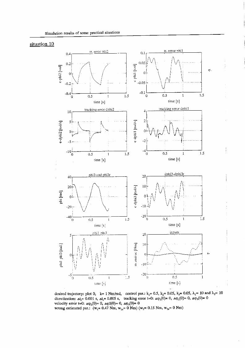
Simulation results of some practical situations
situation 10
F-
ir. error phi? 0.4
N c .- zc
0.5 1 1.5 O 0.5 1 1.5 -0.4 O
time [SI time [s]
tracking error dphi2 4- tracking error dphi l
3 -2 -
-4 - 0.5 1 1.5 o 0.5 1 1.5 -10
O time [SI time [s]
I 20 5 , I
I.
, % ..! I \
I \ I \
I \
10 - .. ' I -I
3 e.*
d i Y
4 2 0- </ - c - -
5% ,.*-._, ! c -10 c..,' . _, -
-?O i
F
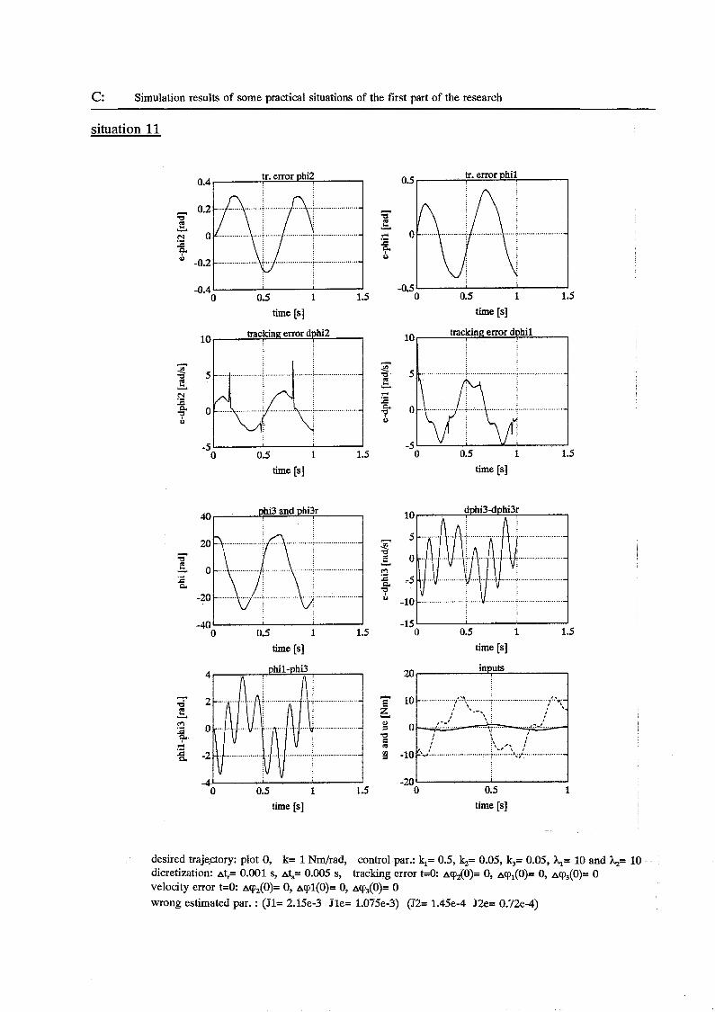
c: Simulation results of some practical situations of the first part of the research
20
- 10 E I . 9 ........... ..............................
;-i, i , *i,- I *--. i
\ : & 5 :
y -10 :km-! ..........
..................... 2 0 _ . _ . . I !.:::..u U
.....- 9
-20
situation 11
0.4
0.2 a" 2 .- N O ..................... Y
c
-0.2
-0.4 O 0.5 1 1.5 O 0.5 1 1.5 time [SI time [SI
O 0.5 1 1.5 O 0.5 1 1.5 time [SI time [SI
time [SI
.....................
-15 O 0.5 1 1.5
time [SI
desired traje-ctory: plot O, k= 1 Nm/rad, dicretization: Atr= 0.001 s, at,= 0.005 s, tracking error t d : acp2(0)= O, ~cp,(O)= O, AQ(O)= O velocity error t=O: ~cp,(O)= O, ~ r p l ( O ) = O, ~ c p , ( O ) = O wrong estimated par. : (J1= 2.i5e-3 Jle= 1.075e-3) (J2= 1.45e-4 J2e= 0.72e-4)
control par.: k,= 0.5, k,= 0.05, k,= 0.05, A,= 10 and &= 10

c: Simulation results of some practical situations of the first part of the research
situation 12 tr. error phi2 o. 1
J O 0.5 1 1.5
time [SI tracking error dphi2
-0.1 '
6
i 4 .................... ..................... t l .............................................
.................... ....................... .....................
O G.5 1 i .5 O G.5 1 i .5
-0.2 1 I O 0.5 1 1.5
time [SI
.....................
U 0.5 1.5 time [SI time [SI
phi3 and phi3r
..................... ..................... -
...................
O 0.5 1 1.5 O 0.5 1 1.5 time [s] time [SI
O 0.5 1 1.5 O 0.5 1 time [SI time [SI
desired trajectory: plot O, dicretization: At,= O.Oo1 s, At,= O.OOS s, velocity error t=O: ~ c p , ( O ) = O, ~ c p í ( O ) = O, ~ c p ~ ( O ) = O wrong estimated par. : k= 1 Nm/rad &= 0.7 Nm/rad
k= 1 Nm/rad, control par.: k,= 0.5, k,= 0.05, k3= 0.05, Al= 10 and %= 10 tracking error t=O: ~cp , (O)= O, ~ c p , ( O ) = O, ~ c p ~ ( O ) = O
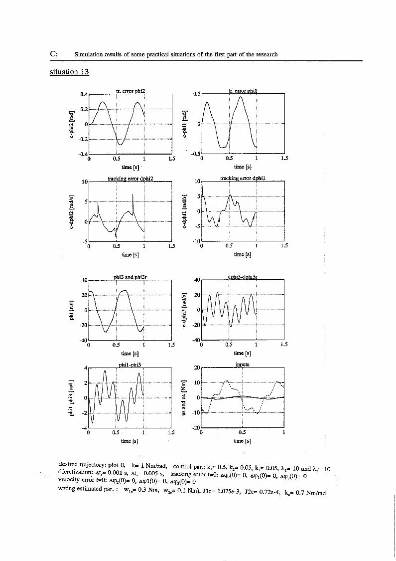
c: Simulation results of some practical situations of the first part of the research
20
- 10 _........ E ..... ............................ ^ .. ,*.y- , .
....... _- , : 3 :
t
z 2 0- _..., !:.:.:.,.* ,.+& U c
situation 13
CJ y -10
-20
.....................
O 0.5 1 1.5 O 0.5 1 1.5 time [SI time [SI
>..( ................................... : \\
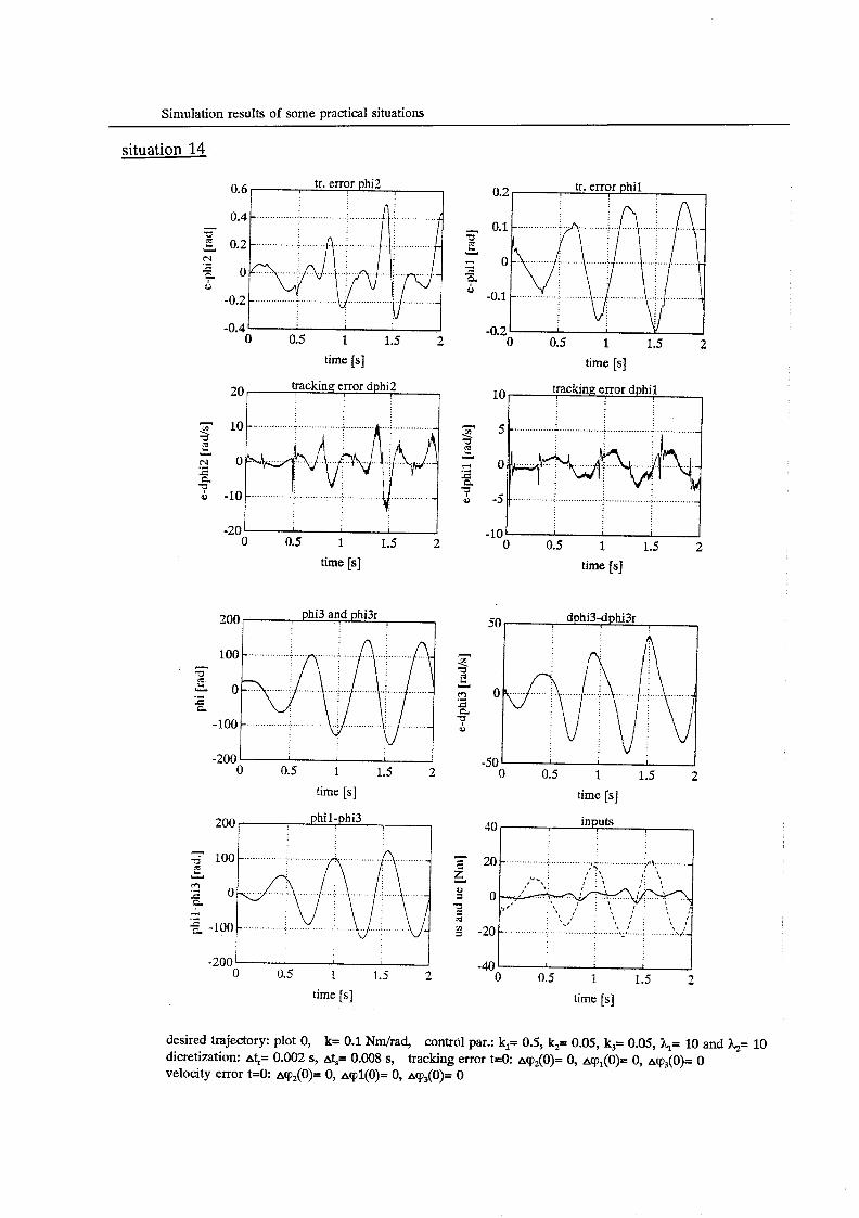
Simulation results of some practical situations
20
-20
-40
situation 14
-. ............. i ............... '._ ................ .ii$... ........ .- ,5, I %
I . , I : , , I
: ', , . , : I
I < , : I <..
I \ . I <:
..., . . . . . . I - ....,......... I j .............
: , I < I L I \ I < I : < I
..... .!. I _
. > . \ , : I 0- : \ , , : , 1 . 8 I' I ! . L I .,
.I - ............................. : ........ :,;; .... 'i.
tr. error phi2 0.6 f I tr. error phi1 0.2 r
...............
...............
-n i ............ ............... ".*
-0.2 O 0.5 1 1.5 2
time [SI
-0.4 I 1 O 0.5 1 1.5 2
time [SI trackine error dphi2 20 i
tracking error dphil 10 1
3
-20 - O 0.5 1 1.5 2
time [SI
phi3 and phi3r 200
-200 - O 0.5 1 1.5 2
time [SI phil-phi3
I
.-
-200 A O 0.5 1 1.5 2
time [s]
c
- P E 3
u m c c,
o
.-
P
3
E
a z u 3
9 .n
-10 - O 0.5 1 1.5 2
time [SI
50 dphi3-dphi3r
-so I I
O 0.5 1 1.5 2 time [SI
desired trajectory: plot O, dicretization: aq= 0.002 s, at,= O.ûû8 s, tracking error t=O: acp,(O)= O, acp,(O)= O, arp,(O)= O velocity error t=O ~cp,(O)= O, ~ c p l ( O ) = O, acp3(0)= O
k= 0.1 Nm/rad, control par.: k,= 0.5, k,= 0.05, k3= 0.05, Al= 10 and &= 10
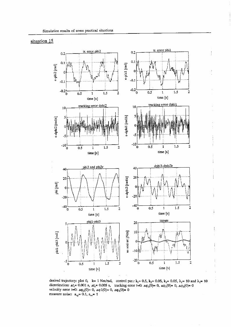
Simulation results of some practical situations
situation 15
..............
- .- r( 0
........ ...........
2 O 0.5 1 1.5 2 -0.2 0.5 1 1.5 O
time [SI time [s]
10 10
5 - e e t! 2 u
c a
3 5 -
o Y .- * o
0 -5
.- N O c
0 -5 a
I I
I , 2 O 0.5 1 1.5 2 -10
O 0.5 1 1.5 -10
time [s] time [SI
time [SI time [s]
time [SI time [SI
desired trajectory: plot O, k= 1 Nm/rad, control par.: kl= 0.5, k2= 0.05, k3= 0.05, hl= 10 and &= 10 dicretization: at;= 0.001 s, at,= 0.005 s, tracking error t=û: ~cp,(O)= O, ~cp,(O)= O, ~ c p @ ) = 0 velocity error t=O: A C ~ ~ ( O ) = 0, ~pl(O)= O, ~ c p , ( O ) = O measure noise: ay= 0.1, aw= 1
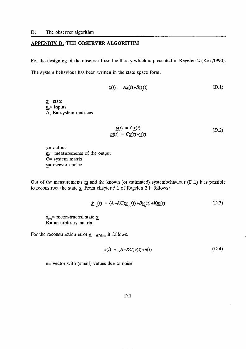
D: The observer algorithm
APPENDIX D: THE OBSERVER ALGORITHM
For the designing of the observer I use the theory which is presented in Regelen 2 (Kok,1990).
The system behaviour has been written in the state space form:
X( t ) - = Ax(t)+Bu - ($1 (D.1) s
- x= state %= inputs A, B= system matrices
y= output E= measureme ts f the output C= system matrix y= measure noise
Out of the measurements to reconstruct the state 5. From chapter 5.1 of Regelen 2 it follows:
and the known (or estimated) systembehaviour (D.l) it is possible
X -rec (t) = (A -KC')X -rec (t) +Bu s (t) +Km(t) - (D.3)
xm= reconstructed state 5 K= an arbitrary matrix
For the reconstruction error e= 5 - ~ it follows:
- e( t) = (A -KC)e( t) +E( t)
- n= vector with (small) values due to noise
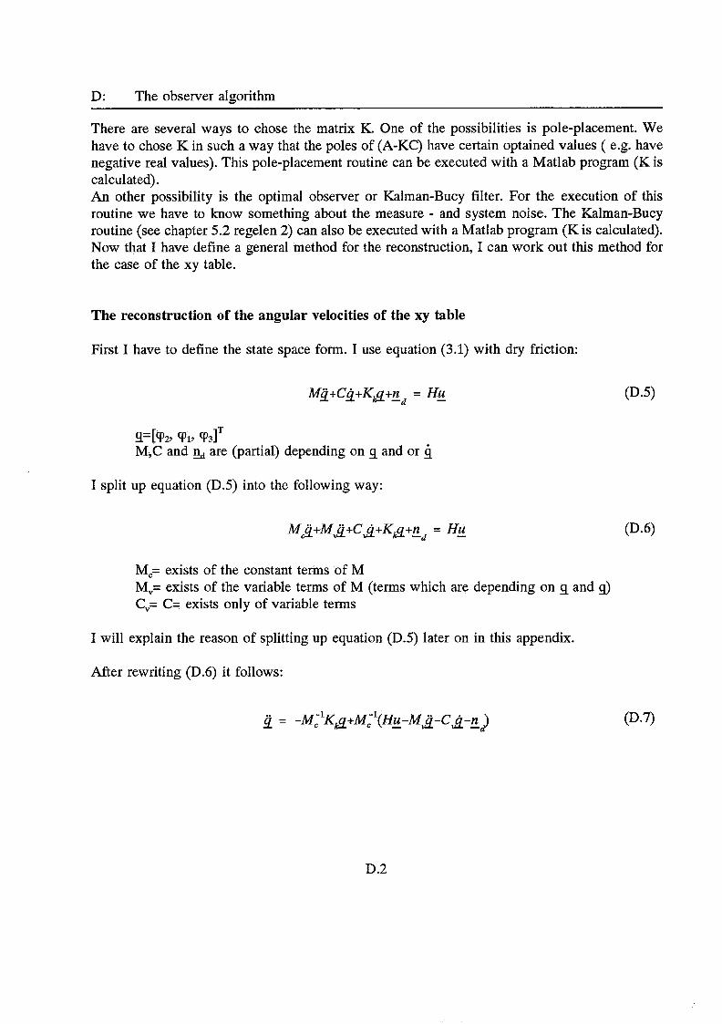
D: The observer algorithm
There are several ways to chose the matrix K. One of the possibilities is pole-placement. We have to chose K in such a way that the poles of (A-KC) have certain optained values ( e.g. have negative real values). This pole-placement routine can be executed with a Matlab program (K is calculated). An other possibility is the optimal observer or Kalman-Bucy filter. For the execution of this routine we have to know something about the measure - and system noise. The Kalman-Bucy routine (see chapter 5.2 regelen 2) can alsi be executed with a Matlab program (R is calculated): Now that I have define a genera! method for the reconstruction, I can work out this method for the case of the xy table.
The reconstruction of the angular velocities of the xy table
First I have to define the state space form. I use equation (3.1) with dry friction:
g'[(PD q 1 7 %IT M7C and n, are (partial) depending on g and or 4
I split up equation (D.5) into the following way:
M,= exists of the constant terms of M M,= exists of the variable terms of M (terms which are depending on 9 and s> Cv= C= exists only of variable terms
I will explain the reason of splitting up equation (D.5) later on in this appendix.
After rewriting (D.6) it follows:
D .2
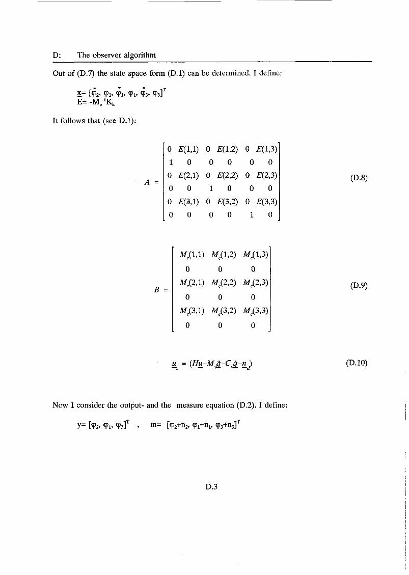
D: The observer algorithm
A =
Out of (D.7) the state space form (D.l) can be determined. I define:
r
O E(1,l) O E(1,2) O E(1,3)
1 0 O 0 O 0
O E(2,l) O E(2,2) O E(2,3)
O 0 1 0 O 0
O E(3,l) O E(3,2) O E(3,3) L 0 0 O 0 1 0
It follows that (see D.1):
(D.lO)
Now I consider the output- and the measure equation (D.2). I define:
Y= CCP2, Vi, %IT 7 m= [V2+n2, CPi+ni, %+n31T
D.3
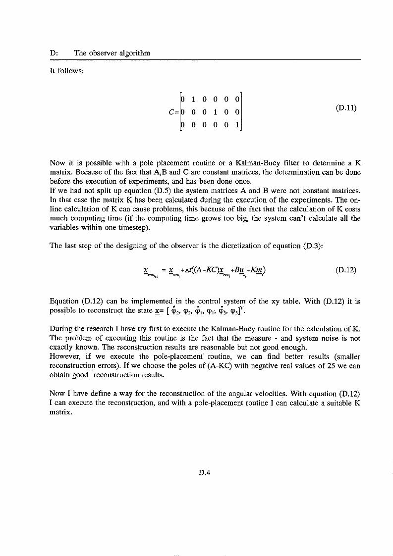
D: The observer algorithm
c=o
It follows:
- 0 1 0 0 0 0
o o 1 o o - 0 0 9 0 0 1 ,
(D.ll)
Now it is possible with a pole placement routine or a Kalman-Bucy filter to determine a K matrix. Because of the fact that A,B and C are constant matrices, the determination can be done before the execution of experiments, and has been done once. If we had not split up equation (D.5) the system matrices A and B were not constant matrices. In that case the matrix K has been calculated during the execution of the experiments. The on- line calculation of K can cause problems, this because of the fact that the calculation of K costs much computing time (if the computing time grows too big, the system can’t calculate all the variables within one timestep).
The last step of the designing of the observer is the dicretization of equation (D.3):
(D.12)
Equation (D.12) can be implemented in the control system of the xy table. With (D.12) it is possible to reconstruct the state &= [ 6 2 7 (p2, GI, cpl, (P3, cp3] T .
During the research I have try first to execute the Kalman-Bucy routine for the calculation of K. The problem of executing this routine is the fact that the measure - and system noise is not exactly known. The reconstruction results are reasonable but not good enough. However, if we execute the pole-placement routine, we can find better results (smaller reconstruction errors). If we choose the poles of (A-KC) with negative real values of 25 we can obtain good reconstruction results.
Now I have define a way for the reconstruction of the angular velocities. With equation (D.12) I can execute the reconstruction, and with a pole-placement routine I can calculate a suitable K matrix.
D.4

E: Simulation - and experimental results of the second part of the research
APPENDIX E: SIMULATION - AND EXPERIMENTAL RESULTS OF THE SECOND PART OF THE RESEARCH
In this appendix I will show some simulation - and experimental results of the second part of the research (see chapter 5).
Situations
I have considered the next desired trajectories:
c> - cp2d= win(m2t) ; 9),<= am2cos(m2t) ; .. min(o,t) ; (Pld= amlcos(mlt) ; .. -
The reference trajectories are showed on page ES - E.7 (1 sec. = 100 timesteps)
I have considered the next situations:
simulation desired trajectory: A, a= 25 rad co= 3.14 rad/s springconstant: k = 0.5 Nm/rad control gain parameters: k,= k2= k3= 0.05, lab,= lab,= 25 observer-poles (used by the pole-placement routine): -25+0.2i
-25+0.3i -25+0.4i
measure frequence: 1/0.01 Herz ( 1 sec. = 100 timesteps) execution time: 2 s position t=O: cpl= ip2= 'p3= O (middle of the xy table) velocity t=O: vi= 'p2= cp3= O particularies: none
E. 1
E: Simulation - and experimental results of the second part of the research
2) As situation 1 but now:
- experiment - execution time: 3.5 s
3) As situation 2 but now:
- - observer-poles: -50+0.2i, -50+0.3i, -50+0.4i -
control gain parameters k,= k2= k3= 0.05, lab,= 50, lab,= 25
measure frequency: V0.007 Herz (1 sec. = 142 timesteps)
4) As situation 2) but now:
- - measure frequency: 1/0.007 Herz (1 sec. = 142 timesteps)
trajectory A, a= 25 rad co= 1.57 rad/§
5) As situation 1) but now:
- trajectory B, a= 25 rad o)= 3.14 rad/s - execution time: 3.5 s
6) As situation 5) but now:
- experiment
7) As situation 1) but now:
- - execution time: 3.5 s
trajectory C, ct= 25 rad o),= 3.14 rad/s, 02= 1.57 rad/s
8) As situation 7) but now:
- experiment - - observer-poles: -50+0.2i, -50+0.3i, -50+0.4i -
control gain parameters k,= k,= k3= 0.05, lab,= 50, lab,= 25
measure frequency: U0.007 Herz ( 1 sec. = 142 timesteps)
E.2
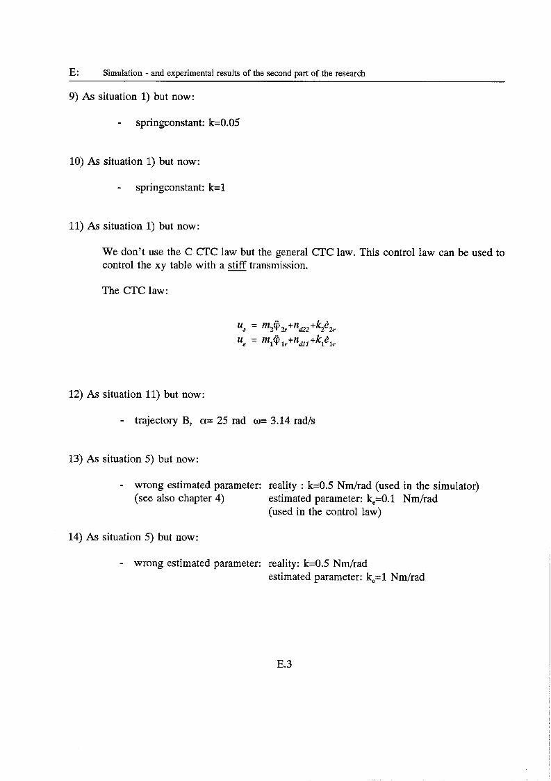
E: Simulation - and experimental results of the second part of the research
9) As situation 1) but now:
- springconstant: k=0.05
10) As situation 1) but now:
- springconstant: k=l
11) As situation 1) but now:
We don’t use the C CTC law but the general CTC law. This control law can be used to control the xy table with a st i f f transmission.
The CTC law:
12) As situation 11) but now:
- trajectory B, a= 25 rad ct)= 3.14 rad/s
13) As situation 5) but now:
- wrong estimated parameter: reality : k=0.5 Nm/rad (used in the simulator) (see also chapter 4) estimated parameter: k,=O.l Nm/rad
(used in the control law)
14) As situation 5) but now:
- wrong estimated parameter: reality: k=OS Nm/rad estimated parameter: k,=l Nm/rad
E.3

E: Simulation - and experimental results of the second part of the research
15) As situation 5) but now:
- wrong estimated parameters:
16) As situation 5) but now:
- wrong estimated parameters:
17) As situation 5) but now:
- wrong estimated parameters:
18) As situation 5) but now:
wrong estimated parameters:
Simulation results
reality: wl= w3= 0.25 Nm, w2= 0.15 Nm estimated parameters: wie= w ~ ~ = 0.1 Nm, wZe= 0.05 Nm
reality: wl= w3= 0.25 Nm, w2= 0.15 Nm estimated parameters: wie= wfe= 0.5 Nm, wze= 0.3 Nm
reality: J,= 2.15 10” kgm’, J,= 1.45 est. par.: Jle= 3 10” kgm’, J,,= 2 lo4 kgm’
kgm’
reality: ms= 2.3 kg, m:= 8.5 kg, me= 2.3 kg est. par.: mse= 3kg, mk= 10 kg, m,= 3 kg
I have made the same plots of every situation as of the theoretical situation (see appendix B). The structure of a page with plots is the same as given in appendix B. Now I will give per situation the simulation results ( see following pages).
E.4
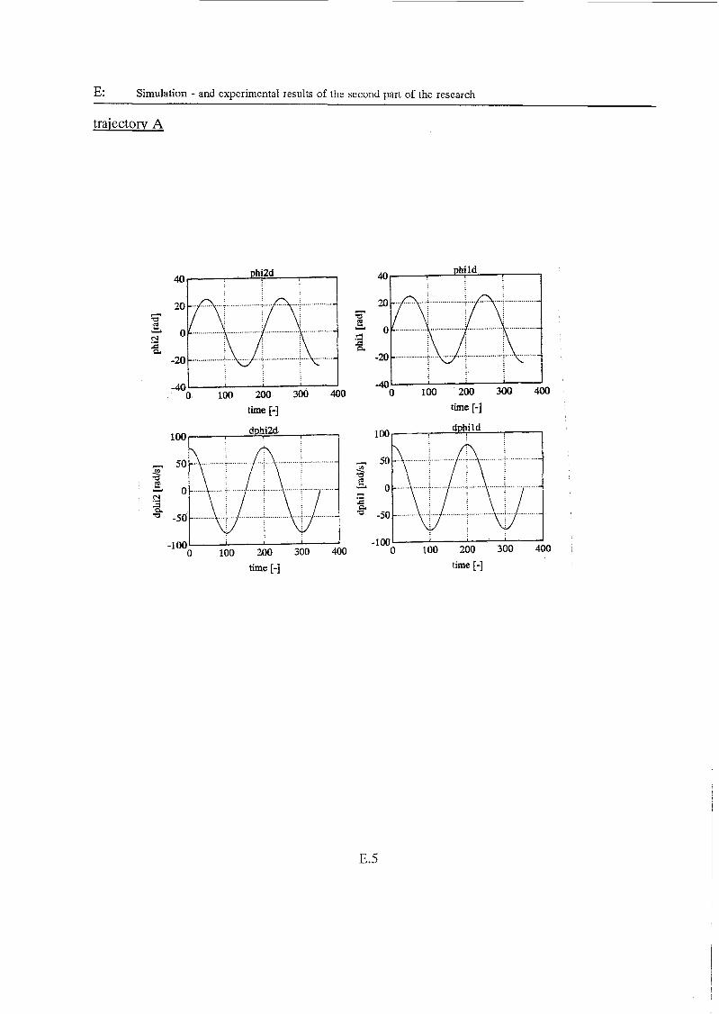
E: Simulation - and experimental results of the second part of the research
trajectory A
-100‘ I o 100 200 300 400 time [-I
o 100 200 300 400 time I-]
o 100 200 300 400 time [-]
o 100 200 300 400 time [-I
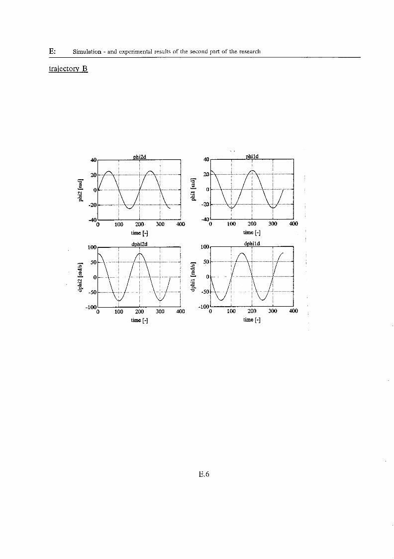
E: Simulation - and experimental results of the second part of the research
trajectory B
o 100 200 300 400 o 100 200 300 400 time E-] time [-J
O 100 200 300 400 o 100 200 300 400 time [-] time [-I
E. 6
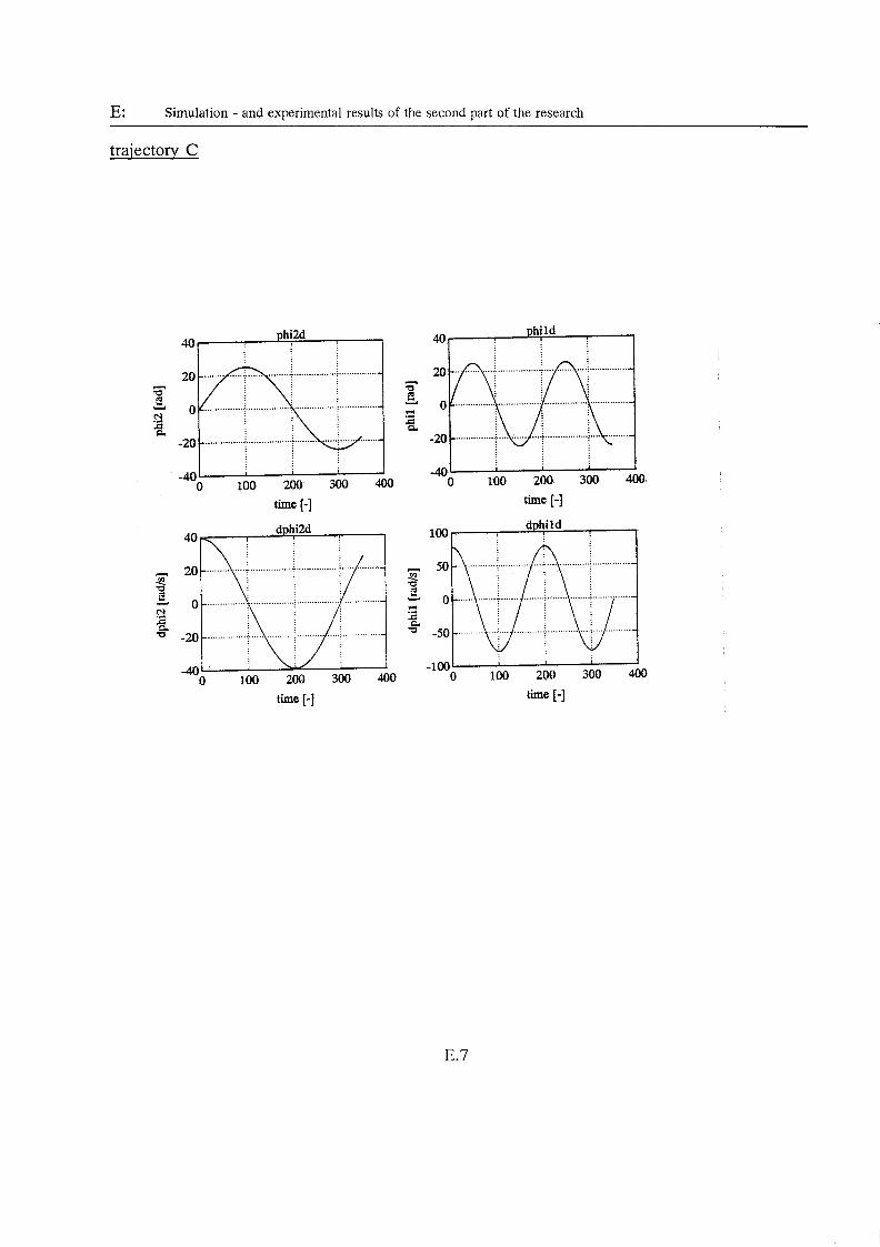
E: Simulation - and experimental results of the second part of the research
trajectory C
phi2d 40
z e Y
.-(
E a .-
-40‘ I o 100 200 300 400
time [-I dphi2d 40 1
20 ......... ___.i ................ :: ................. .............. I/, ; E ............... \ ................. ................. p ..............
100 200 300 400 time [-I
o 100 200 300 400 time [-I
.loo - o 100 200 300 400 time [-I
E.7
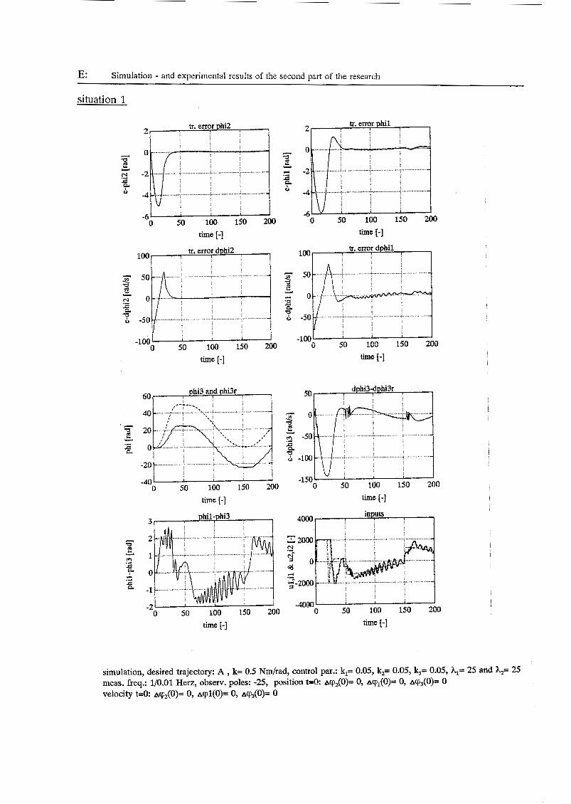
E: Simulation - and experimental results of the second part of the research
...._..........<i ............................... -
................. i.... ............ :; ............... -
situation 1
tr. error phi2 2
time [-I tr. error dohi2 1001 1
-100- O 50 100 150 200 time [-I
phi3 and phi3r 60 --*-__
I . . : I : . .
, : . . 40 .......................... A . . ...... ............................
50 100 150 200 -40
O time E-]
phil-phi3 i
time [-I
rl c a z
w
time [-I
-100' i
V 50 100 I50 200 time [-I
O 50 100 150 200 time [-I inputs
4000
I 50 100 150 200
-4000l O
time [-I
simulation, desired trajectory: A , k= 0.5 Nm/rad, control par.: k,= 0.05, kz= 0.05, k,= 0.05, h,= 25 and &L= 25 meas. freq.: 1/0.01 Herz, observ. poles: -25, position t=O ~cp, (O)= O, ~ c p ~ ( O ) = O, A%(O)= O velocity t=O: ~cp~(û)= O, ~ c p l ( O ) = O, ~cp , (O)= O

E: Simulation - and experimental results of the second part of the research
situation 2
o 100 200 300 400 time [-I
z e c e Y
+
0
tr. error hi1 5
0 ........... ...............
-5 ................ .................................
v i
-10 o 100 200 300 400 time [-]
tr. error dphi2 100
-50 .................. ! ............... ................. ! ........... a
I
O 100 200 300 400 O 100 200 300 400 -100
time [-] time [-I
O 100 200 300 400 O 100 200 300 400 time E-] time [-]
O 100 200 300 400 O 100 200 300 400 time [-I time [-J
experiment, desired trajectory: A , k= 0.5 Nm/rad, control par.: k,= 0.05, k,= 0.05, k3= 0.05, &= 25 and &= 25 meas. freq.: 1/0.01 Herz, observ. poles: -25, position t=O: ~cp, (O)= O, ~ c p , ( O ) = O, acp3(0)= O velocity t=O ACP,(O)= O, ~ c p l ( O ) = O, ~ c p , ( O ) = O

E: Simulation - and experimental results of the second part of the research
Y
N a -50 a .-
7 -100 ...................................................................... -
_. ................................................................... -
-100
dphi3dphi3r 400 phi3 and phi3r 200
150 ........................................................ ~~~
- : '* 100 ........ ....................................................
500 -600
500 O time [-I time [-I
-50 O
.......................
................................. ........................
O 500 O 500 time (-1 time [-I
experiment, desired trajectory: A , k= 0.5 Nmhad, control par.: k,= 0.05, k,= 0.05, k3= 0.05, hl= 50 and b= 25 meas. freq.: 1/0.007 Herz, observ. poles: -50, position t=O: ~cp, (O)= O, ~rp,(O)= O, ~ c p , ( O ) = O velocity t=O ~cp,(û)= O, ~ c p l ( O ) = O, ~ c p , ( O ) = O

E: Simulation - and experimental results of the second part of the research
situation 4
tr. error phi2 1
0 ............................................................
-1 ...................................................................
-2
-3
I F .................................................................... 1 H 1
O 500 time [-I
tr. error dphi2 so I 1
-100 O 500
time [-]
phi3 and phi3r 40 1
c a
-40 ' I O 500
time [-I phi 1-phi3 1.5
f I
-1 - O 500
time [-I
2 tr. error phi1 I
O 500 time {-I
tr. error dphil 50
............................. .k-
....................................... -
-100 + o 500
time [-I
50 dphi34phi3r I
U f! u -50 .- E a
-150' I O SO0
time [-I
7 2000 I
-2000' I O 500
time [-I
experiment, desired traj: A with w=1.57, k= 0.5 Nm/rad, control par.: kl= 0.05, k2= 0.05, k3= 0.05, hl= 25 and &= 25 meas. freq.: 1/0.007 Herz, observ. poles: -25, position t=& acp,(O)= o, acp,(O)= o, AT,(o)= 0 velocity t=& ~cp,(û)= 0, ~ r p l ( O ) = O, acp3(û)= O

E: Simulation - and experimental results of the second part of the research
................................... 1 .............
...... _ ................. ..................
-100
situation 5
û Ì? Y
(v
E .- 2
tr. error phi1 20 I
O 200 400 600 800 O 200 400 600 800 time [-] time [-I
600 800 O 200 400 600 800 time [-3 time [-]
simulation, desired trajectory: B , k= 0.5 Nm/rad, control par.: k,= 0.05, k2= 0.05, k3= 0.05, meas. freq.: 1/0.005 Herz, observ. poles: -25, position t=O ~cp,(O)= O, acp,(O)= O, acp3(Q)= 0 velocity t=O: AV@)= O, ~ ' p l ( O ) = O, ~ c p , ( O ) = O
25 and %= 25
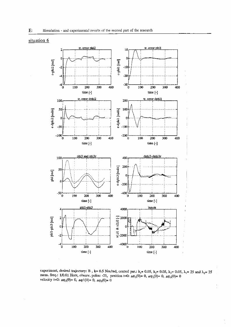
E: Simulation - and experimental results of the second part of the research
a F -50
situation 6
................................... ; ................... I
tr. error phi2 2 1
I , : > , : I , : I I :
I , : 5 ,
....................... : .................. :
O 100 200 300 400 time [-]
tr. error dphi2 100 1
time 1-1
phi3 and phi3r 100, i
time 1-1 phil-phi3 4 1
O 100 200 300 400 time [-I
-30 I O 100 200 300 400
time [-3 tr. error dphil 200, 1
O 100 200 300 400 time [-I
dphi3-dphi3r 400 1
time [-I inputs 4Ooo
z 2000 N Ni = o 4 * .- 2-2000
-4000 ' I o loo 200 300 400 time [-I
experiment, desired trajectory: B , k= 0.5 Nm/rad, control par.: k,= 0.05, k,= 0.05, k,= 0.05, hl= 25 and &= 25 meas. freq.: 1/0.01 Herz, observ. poles: -25, position t=O: ~cp, (O)= O, ~ c p , ( O ) = O, ~cp,(O)= O velocity t=O: ~cp, (O)= O, ~ r p l ( O ) = O, ~ c p , ( O ) = O
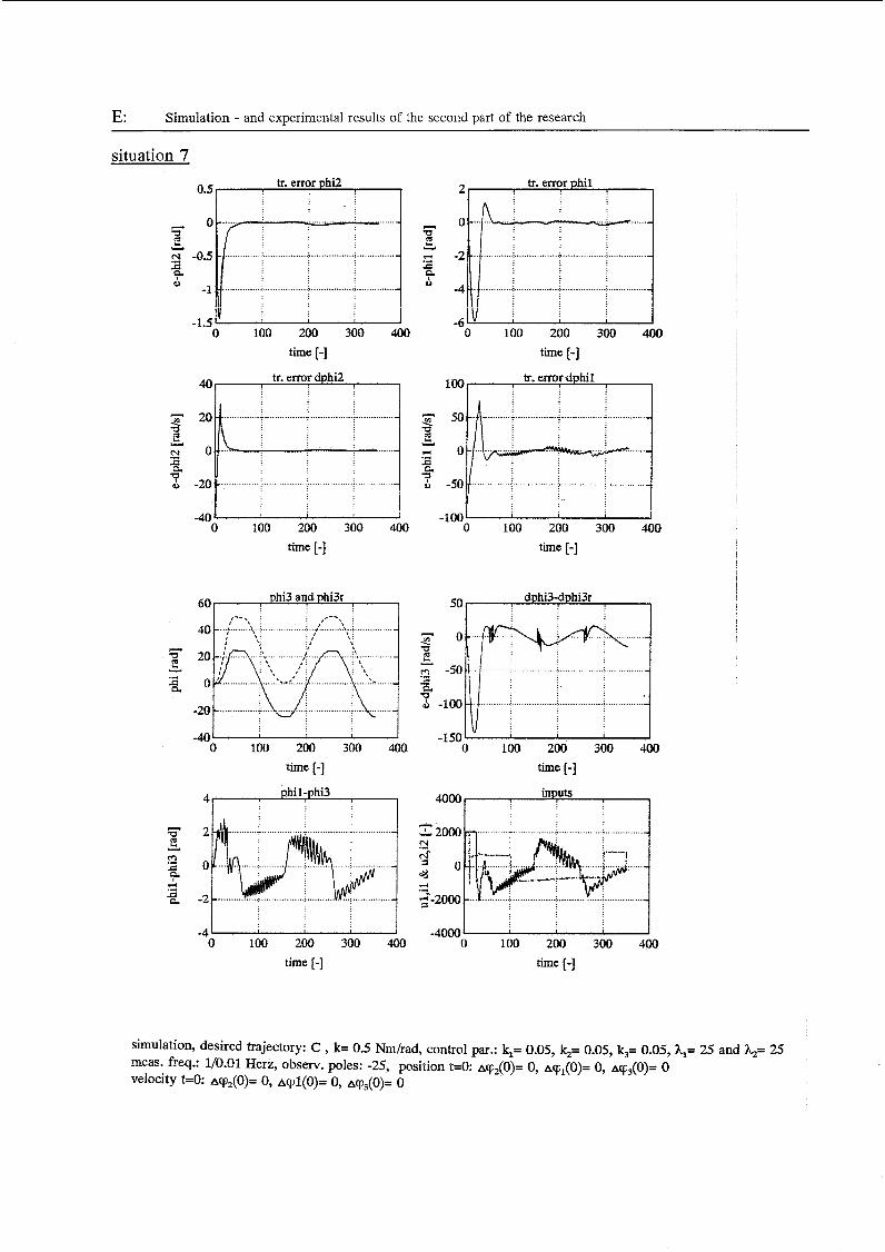
E: Simulation - and experimental results of the second part of the research
...... -
~~
situation 7 tr. error phi2 0.5 r I
time [-I time [-I tr. error dphil 100 tr. error dphil 40 I
time [-] time 1-3
phi3 and phi3r I
-40 I O 100 200 300 400
time [-I time [-]
I - -40000 200 300 400
-41 O 100 200 300 400
time (-1 time [-I
simulation, desired trajectory: C , k= 0.5 Nm/rad, control par.: k,= 0.05, k,= 0.05, k3= 0.05, LI= 25 and &= 25 meas. freq.: 1/0.01 Herz, observ. poles: -25, position t=O AT,(O)= O, ~ c p , ( O ) = O, acp,(O)= 0 velocity t=O ~rp,(O)= O, ~ c p l ( O ) = O, ~ c p , ( O ) = O
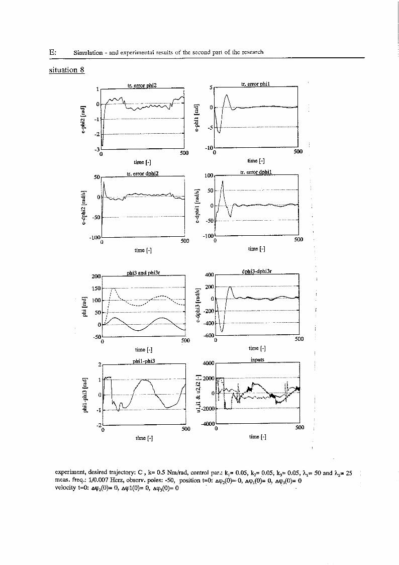
E: Simulation - and experimental results of the second part of the research
. . . . . . . . . . . . . . . . . . . -8
.......................................... -
situation 8
tr. error phi2 1,
0 ...............................................................
~ -1 ................................................................... 2
8 . u
.... - E l r n ...................................................................
i .? -2 [ IJ I
I
500 -3 '
O
F ì2 Y
r(
c .d a a i
I
500 -10
O
dphi3-dphi3r 200 phi3 and phi3r 400
150 ................................................................ -
500 -600 -
500 O time (-1 time [-I
-50 O
500 O 500 O time [-I time [-I
experiment, desired trajectory: C , k= 0.5 Nm/rad, control par.: kl= 0.05, k2= 0.05, k3= 0.05, hl= 50 a d &= 25 meas. freq.: 1/0.007 Herz, observ. poles: -50, position t=O: ~cp, (O)= O, ~ c p , ( O ) = O, acp,(O)= O velocity t=O: ~rp,(O)= O, ~ c p l ( O ) = O, ~cp , (O)= O
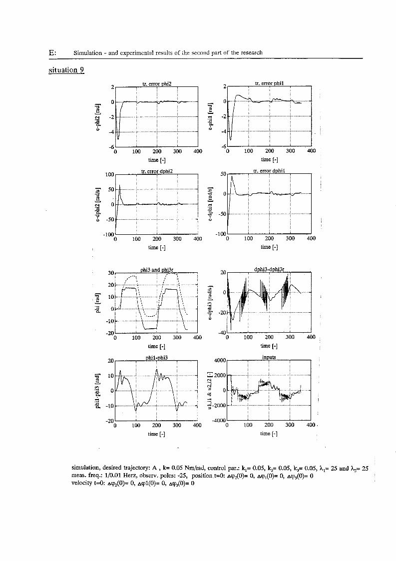
E: Simulation - and experimental results of the second part of the research
I "
situation 9
-;-2000 a -.I ............. ;.. . . . . . . . . . . .<<...I .................. ,
-1001 I O 100 200 300 400
time [-I
û i! Y .- c a
phi3 and phi3r 4 ,- - : I 4, : ' :< : I :>
,<-.- 30
20 : , 3 ;
......... .:.. ...... ....: ....,... ......... ;! ,. ........... -
-20 O 100 200 300 400
5- ;3 Y
tr. error phi1
O 100 200 300 400 time [-I
- e E Y
m c c. .-
time [-I
20
O
-20
I O 100 200 300 400
simulation, desired trajectory: A , k= 0.05 Nm/rad, control gar.: k,= 0.05, k2= 0.05, k3= 0.05, hl= 25 and &= 25 meas. freq.: 1/0.01 Herz, observ. poles: -25, position t=O: AqP2(0)= o, Aqp,(O)= o, AT@)= 0 velocity t=O: ~cp , (O)= O, ~ c p í ( O ) = O, acp,(O)= O

E: Simulation - and experimental results of the second part of the research
situation 10
O 100 200 300 400 O 100 200 300 400 time [-I time [-I
-1001 -100 - O 100 200 300 400 o 100 200 300 40'
time [-I time [-I
-40 - O 100 200 300 400
time [-]
phil-phi3 3
2 t .......................................................... . .
-2 - O 100 200 300 400
time [-I
dphi3-dphi3r 1
-200 I I 0 100 200 300 400
time I-] inputs 4000
......................
-4000 I I O 100 200 300 400
time [-I
simulation, desired trajectory: A , k= 1 Nm/rad, control par.: k,= 0.05, k,= 0.05, k,= 0.05, hl= 25 and &= 25 meas. freq.: 1/0.01 Herz, observ. poles: -25, position t=O: ~ c p , ( O ) = O, acpI(O)= O, ~ c p , ( O ) = O velocity t=O: AC@)= o, ~ c p l ( O ) = O, a(p3(O)= O
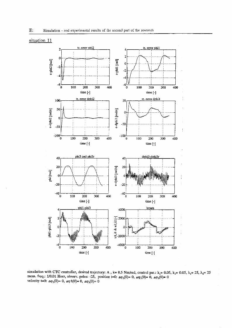
E: Simulation - and experimental results of the second part of the research
-50
situation 11
._ ............... ; ............... + ...................... ..........._
O 100 200 300 400 o 100 200 300 400 time [-I time [-I
tr. error dphi2 1001 1
- 50 ............. ............. ...; .......................... e 2
3 2
z Y
U
ri
a
Y
.- c a -50 ............................ ............ . _
-100- - O 100 200 300 400
time [-I time [-I
O 100 200 300 400 O 100 200 300 400 time [-I time [-I
-4 ' I
O 100 200 300 400 O 100 200 300 400 time E-] time [-I
simulation with CTC controller, desired trajectory: A , k= 0.5 Nmhad, control par.: k,= 0.05, k2= 0.05, hl= 25, &= 25 meas. freq.: 1/0.01 Herz, observ. poles: -25, position t=O ~cp,(O)= O, ~ c p , ( O ) = O, AT@)= 0 velocity t=O: ~cp,(O)= O, ~ c p î ( O ) = O, ACP,(O)= O

.I c a X -50
~
O 100 200 300 400 O 100 200 300 400 ~
time [-1 time [-3
I O 100 200 300 400
-4 L O 100 200 300 400
time [-I time [-I
__.__.__.~ ___.........._.__ _.._ ._.__....__._ i
simulation with CTC controller, desired trajectory: B , k= 0.5 Nm/rad, control par.: k,= 0.05, k2= O.O§, A,= 25, &= 25 meas. freq.: 1/0.01 Herz, observ. poles: -25, position t = o acp,(O)= O, ~cp,(O)= O, ~cp,(O)= O velocity t=O: ACP,(O)= O, ~ c p l ( O ) = O, ~cp,(O)= O
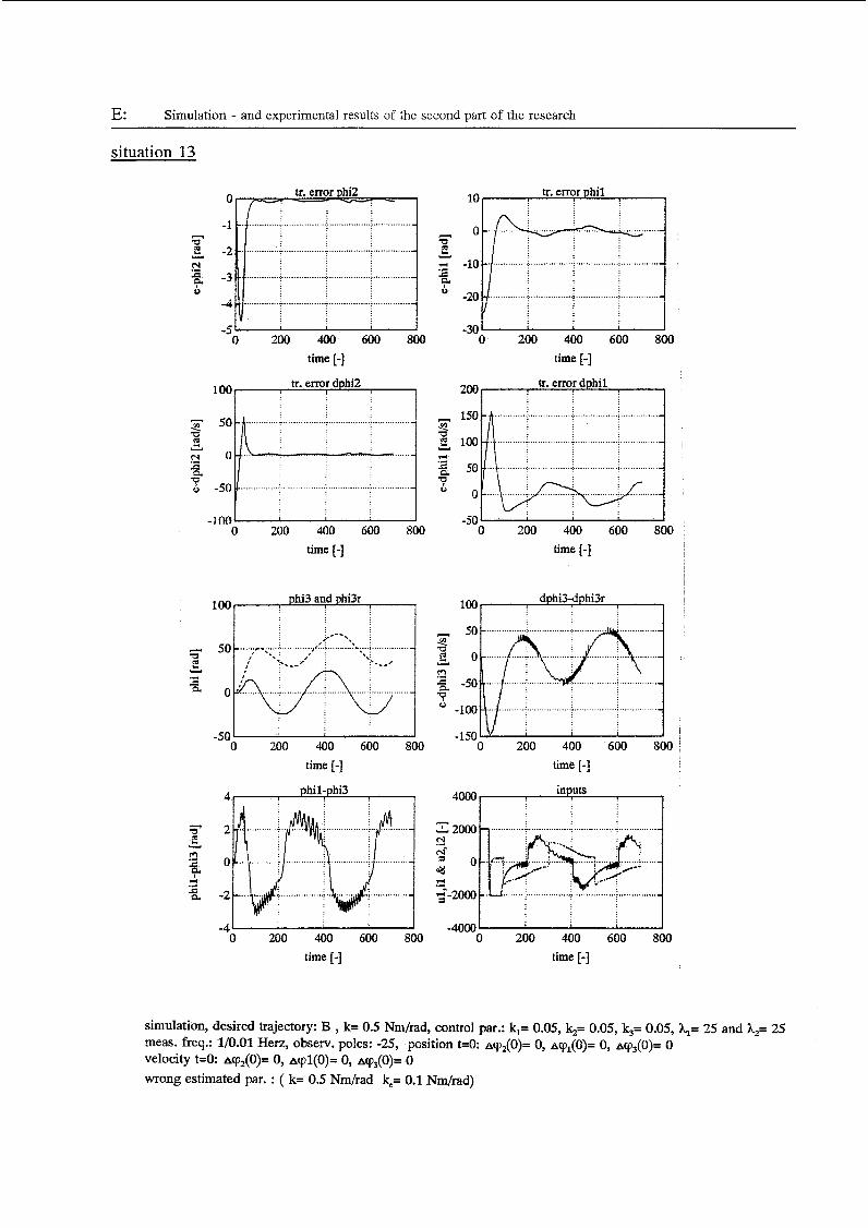
E: Simulation - and experimental results of the second part of the research
situation 13
û E -2 .............i. ................ ................. ...............
.......... ...............
10
O û E r( -10
-20
Y
.- c a 0
1 -30 O 200 400 600 800
time [-I tr. error dphi2 100
a ì
tr. error phi1 1
200 400 600 800 time [-3
-100' -50 ' I O 200 400 600 800 O 200 400 600 800
time 1-1 time [-3
dphi34phi3r I 100 phi3 and phi3r 100 I
O 200 400 600 800 time [-I time [-3
O 200 400 600 800 O 200 400 600 800 time [-I time [-I
simulation, desired trajectory: B , k= 0.5 Nm/rad, control par.: k,= 0.05, k2= 0.05, k3= 0.05, A,= 25 and &= 25 meas. freq.: 1/0.01 Herz, observ. poles: -25, position t=O: ~cp, (O)= O, acp,(O)= O, acp,(O)= O velocity t=O acp2(û)= O, ~ c p l ( O ) = O, acp,(O)= O wrong estimated par. : ( k= 0.5 Nm/rad &= 0.1 Nm/rad)
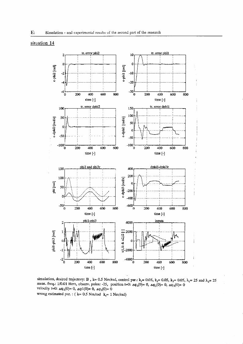
E: Simulation - and experimental results of the second part of the research
situation 14
ü O[. IjTl ......
ì2 N -2 ............... j_ ................ ................. i ...............
F
Y
.-
4 -41 ................................ : ................................. c
I " I
10
O z ì2 + -10 3 9
-20
Y
8
- O 200 400 600 800
time [-3 tr. error dphi2 100
o 200 400 600 800 time [-I
phi3 and phi3r 150
.................................................
..... ...........................
.....
-50' I O 200 400 600 800
time [-]
phil-phi3 1
b Y
m .- c o F
a -1 r(
c .-
-2' I O 200 400 600 800
time [-I
-30 O 200 400 600 800
time [-]
tr. error dphil 150 I i
time [-I
dphi3dphi3r 400 I
O 200 400 600 800 time [-I inputs 4000 1
-4000 O 200 400 600 800
time [-I
simulation, desired trajectory: B , k= 0.5 Nm/rad, control par.: k,= 0.05, k2= 0.05, k,= 0.05, hl= 25 and &.= 25 meas. freq.: 1/0.01 Herz, observ. poles: -25, position t=O: Acp2(0)= o, Acpi(o)= o, AV@)= 0 velocity t=& ~cp,(O)= O, ~ c p i ( O ) = O, acp,(O)= O wrong estimated par. : ( k= 0.5 Nm/rad k,= 1 Nm/rad)
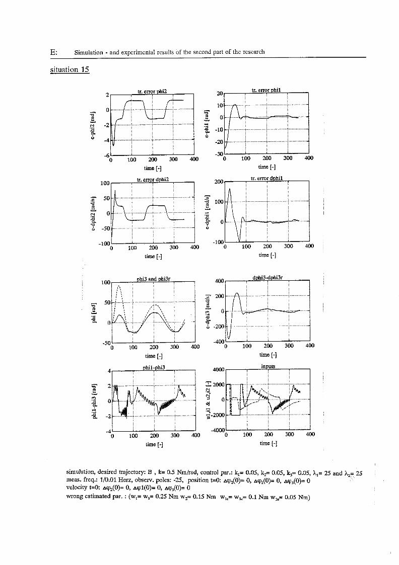
E: Simulation - and experimental results of the second part of the research
situation 15
0 .............................. .;, ............................... -
o 100 200 300 400 o 100 200 300 400 time [-] time [-I
tr. error dphil I
tr. error dphi2 100r
-1001 I
o 100 200 300 400 o 100 200 300 400 time [-I time [-I
phi3 and phi3r 100 ;I, i
-501 1 O 100 200 300 400
time [-I time [-I
o 100 200 300 400 time [-] time [-I
simulation, desired trajectory: B , k= 0.5 Nm/rad, control par.: kl= 0.05, k2= 0.05, k,= 0.05, hl= 25 and b= 25 meas. freq.: 1/0.01 Herz, observ. poles: -25, position t=O ~ c p , ( O ) = O, ~ c p , ( O ) = O, ~cp , (O)= O velocity t=& ~cp,(o)= 0, ~ c p î ( O ) = O, ~ c p , ( O ) = O wrong estimated par. : (wl= w,= 0.25 Nm w2= 0.15 Nm wlc= w%= 0.1 Nm wZ= 0.05 Nm)

E: Simulation - and experimental results of the second part of the research
situation 16 tr. error phi2 4 , 1
o 100 200 300 400 time [-] time [-I
O 100 200 300 400 o 100 200 300 400 time [-] time [-]
7 s z Y
a
phi3 and phik 100 I I
-50 I O 100 200 300 400
400, dphi3-dphi3r
o 100 200 300 400 time E-] time [-I
4000
z 2000 N .- $ 0 4 r( .- 5-2000
-4000 o 100 200 300 400 O 100 200 300 400 time [-I time [-I
simulation, desired trajectory: B , k= 0.5 Nm/rad, control par.: kl= 0.05, k2= 0.05, k3= 0.05, hl= 25 and &= 25 meas. freq.: 1/0.01 Herz, observ. poles: -25, position t=O: ~ c p ~ ( O ) = O, ~ c p , ( O ) = O, ~ c p , ( O ) = O velocity t=& AC@)= O, ~cpl(O)= O, ~cp,(O)= O wrong estimated par. : (wi= w3= 0.25 Nm w2= 0.15 Nm wlc= wse= 0.5 Nm wk= 0.3 Nm)

E: Simulation - and exDerimenta1 results of the second part of the research
situation 17 tr. error phi2
...... - G E c? Y
-4 .............. ....................... ! ............... -
-6
E
?
o 100 200 300 400 o 100 200 300 400 time [-I time [-]
100 - tr. error dphi2
......
a ................ ...... ...........i ..................
tr. error dphi2 100
-100- o 100 200 300 400 time [-I time (-1
phi3 and phi3r 1óO I-* : , I . I k - , I : , I
$ 8 : ................. 50 -; ..... ....... : .................. : ..............._
-50 O 100 200 300 400
dphi3dphi3r 400
o 100 200 300 400 time [-] time [-I
,
I
,
o 100 200 300 400 o 100 200 300 400 time [-I time (-1
simulation, desired trajectory: B , k= 0.5 Nm/rad, control par.: k,= 0.05, k2= 0.05, k,= 0.05, &= 25 and &.= 25 rneas. freq.: 1/0.01 Herz, observ. poles: -25, position t=O: ~cp,(O)= O, ~ c p , ( O ) = O, acp,(O)= O velocity t=O: acpZ(O)= O, ~ c p l ( O ) = O, acp,(O)= Ca wrong estimated par. : (J1= 2.15e-3, J,= 1.45e-4 J1,= 3e-3 Ja= Ze-4)
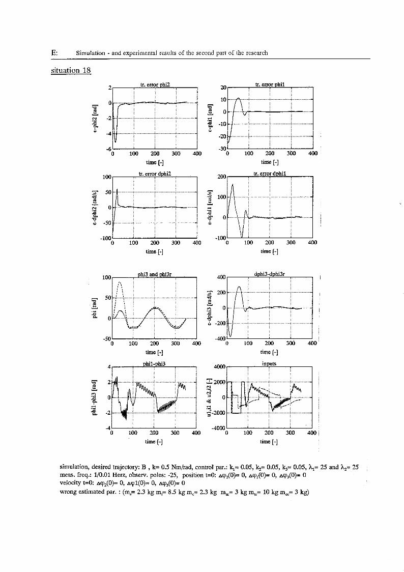
E: Simulation - and experimental results of the second part of the research
situation 18
T 6 Y .- E p.
Y
m E .- I. z a
o 100 200 300 400 time [-]
-100' 1 o 100 200 300 4oQ
time [-I
o 100 200 300 400 time [-I
tr. error dphil 1
time [-3
phi3 and phi3r
-200
-400
..._ ...........,.i .........,........ i ................. ~
J o 100 200 300 400'
-50 o 100 200 300 400
time [-I phil-phi3 4, I
-4 ' I O 100 200 300 400
time [-I
dphi3-dphi3r 400, 1
time [-I
-4000 I I o 100 200 300 400 time [-I
simulation, desired trajectory: B , k= 0.5 Nm/rad, control par.: k,= 0.05, k,= 0.05, k,= 0.05, &= 25 and &= 25 meas. freq.: 1/0.01 Herz, observ. poles: -25, position t=O: ~ c p , ( O ) = O, ~ c p , ( O ) = O, aq,(O)= O velocity t=O: ~ c p , ( O ) = O, ~ c p l ( O ) = O, ~cp,(O)= O wrong estimated par. : (ms= 2.3 kg mt= 8.5 kg me= 2.3 kg msc= 3 kg mte= 10 kg me= 3 kg)
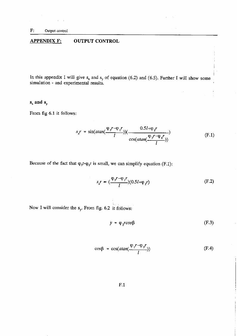
F: Output control
APPENDIX F OUTPUT CONTROL
I Iii this appeiidiri I =ill give s, and sy of equation (ó.2j and (6.5) Further I wiii snow some , simUl2ttiûii - aiid eripeniiieiiíal mulis.
s, and s,
From fig 6.1 it follows:
Q.51+cp2r
>> cp 3r-cp I>( cp3r-cp sxr = sin(atan(
1 cos( atan(
I
Because of the fact that cp3r-cplr is small, we can simplify equation (F.1):
Now I will consider the s,,. From fig. 6.2 it follows:
y = cp2rcosp
>> cp 1Y-T fr E
cosp = cos(atun(
F. a
F: Output control
Because of the fact that cp3r-cp,r is small, we can simplify equation (F.4):
This leads to:
In the on-line generation routine of qld and cp2d (6.2, 6.5 and 6.6 and 6.7 ) I have used s, and sy of equation (F.2) and (F.6). We have to derivate s, and s, twice (to calculate ?d, ?d and fd, ?,J. If we had use F.1 anf F.3 we, get long terms, ~~ this ~- Iead to pmblems during t&i~e~~it t ioi of experiments ( computing time can grow too big).
- i ~~~
Simulationresults
I have considered the next situations:
simulation desired trajectory: xd= asin(cr>t) Yd= min(ot) a= 25 rad co= 3.14 rad/s springconstant: k = 0.5 Nm/rad control gain parameters: k,= k,= k3= 0.05, lab,= lab,= 25 observer-poles (used by the pole-placement routine): -25+0.2i
-25+0.3i -25+0.4i
measure frequency: 0.01 s execution time: 3.5 s position t=O: (pi= cp2= cp3= O (middle of the xy table) velocity t=O: 'pi= cp,= cp3= O particularies: no on-line generation of (P1d and (P2d
Note: This is the same situation as situation 1 of appendix E.
F.2
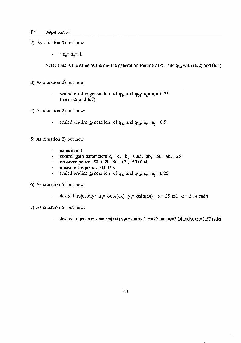
F: Output control
2) As situation 1) but now:
- : ax= ay= 1
Note: This is the same as the on-line generation routine of T1d and T,d with (6.2) and (6.5)
3) As situation 2) but now:
- scaled on-line generation of and T2d: ax= ay= 0.75 ( see 6.6 and 6.7)
4) As situation 2) but now:
- scaled on-line generation of T1d and T2d: ax= ay= 0.5
5) As situation 2) but now:
- experiment - - observer-poles: -50+0.2i, -50+0.3i, -50+0.4i - measure frequency: 0.007 s -
control gain parameters k,= k2= k3= 0.05, lab,= 50, lab,= 25
scaled on-line generation of cpld and vu: ax= ay= 0.25
6) As situation 5) but now:
- desired trajectory: xd= acos(ot) yd= crsin(ot) , a= 25 rad o= 3.14 rad/s
7) As situation 6) but now:
- desired trajectory: xd=acos(o&) yd=asin(02t), a=25 rad 01=3.14 rad/s, m2=î.57 rad/s
F.3
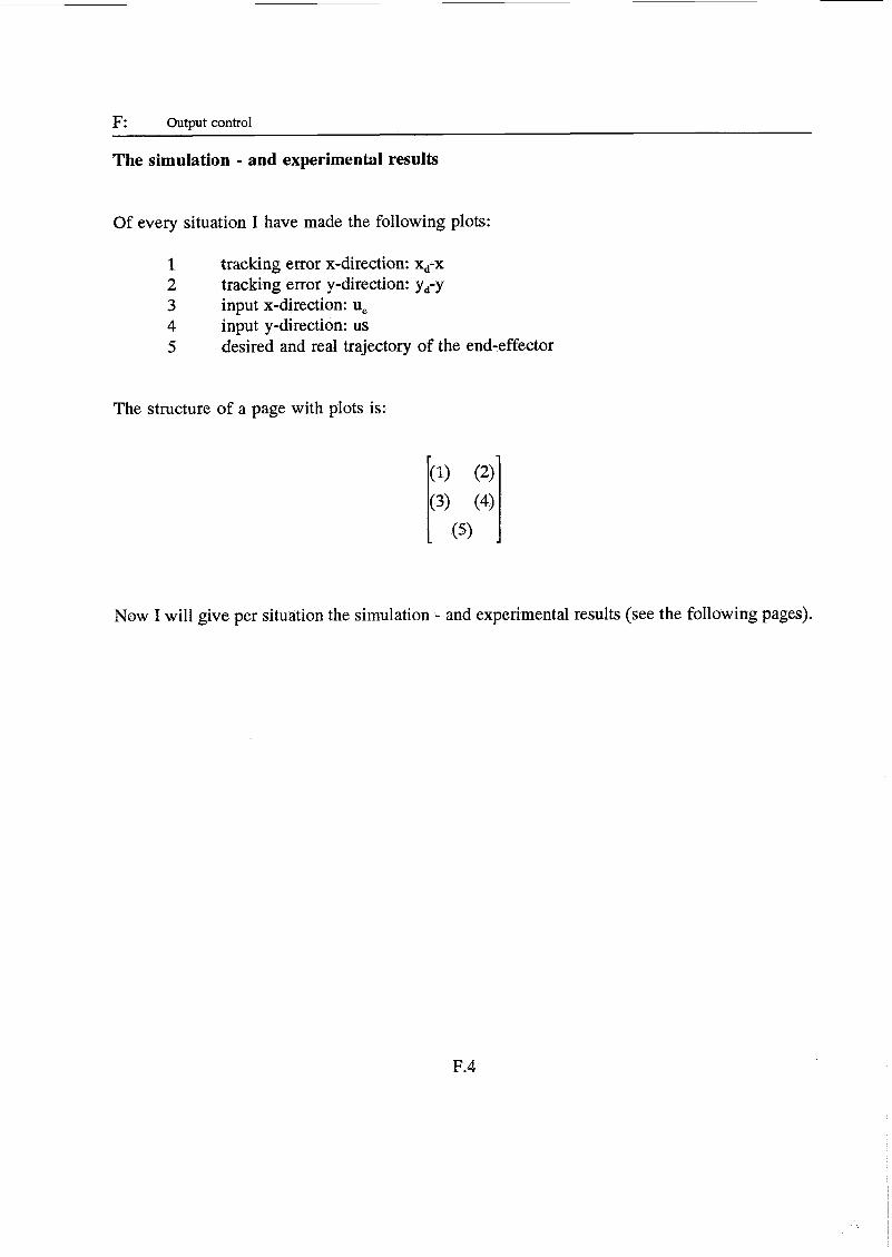
F: Output control
The simulation - and experimental results
Of every situation I have made the following plots:
1 tracking error x-direction: x,-x 2 tracking error y-direction: y,-y 3 input x-direction: u, 4 input y-direction: us 5 desired and real trajectory of the end-effector
The structure of a page with plots is:
Now I will give per situation the simulation - and experimental results (see the following pages).
F.4

F: Results of the controlling of the erid-effector of the xy table
situation 1
- o o u
- Y
&
-6 I o loo 200 300 400
time [-I time [-I
O 100 200 300 400 time [-I time [-]
e.e. path
x-pos [cm]
simulation, desired trajectory: xd= 25sin(3.14t) yd= 25sin(3.14t), k= 0.5 Nm/rad, control par.: kl= 0.05, k,= 0.05, k3= 0.05, hl= 25 and &= 25 meas. freq.: 1/0.01 Herz, observ. poles: -25, position t=O: ~cp,(o)= o, aV,(O)= o, AT,(O)= 0 velocity t=& ~cp,(O)= O, ~cpl(O)= O, ~cp,(O)= O, ax= ay= O
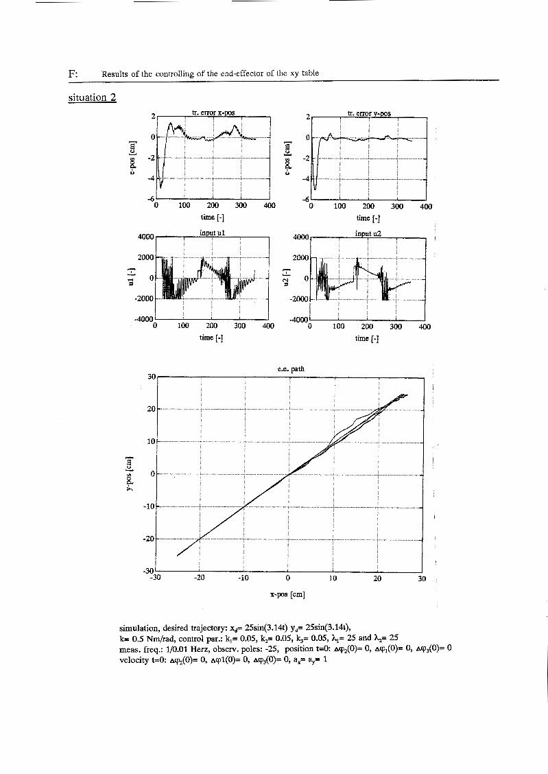
F: Results of the controlling of the end-effector of the xy table
situation 2
- E o Y
E e,
tr. error x-pos 1
o 100 200 300 400
tr. error y-pos 2
o 100 200 300 400 time [-I input u2 4000 I
time [-I input u1
- -40000 100 200 300 400
time [-I
30 I
20 I E o
0 ........................
& x : I -10 .........................
-20 ........................ i /
-4000 - o 100 200 300 400 time [-I
e.e. path
-30 I I -io O 10 20 30 -30 -20
simulation, desired trajectory: x,= 25sin(3.14t) y,,= 25sin(3.14t), k= 0.5 Nm/rad, control par.: k,= 0.05, k,= 0.05, k3= 0.05, Al= 25 and &= 25 meas. freq.: 1/0.01 Herz, observ. poles: -25, position t=O ~cp,(O)= O, acp,(O)= O, acp,(O)= O velocity t=O: ~cp,(O)= O, ~cpl(O)= O, acp3(0)= O, ax= a,,= 1
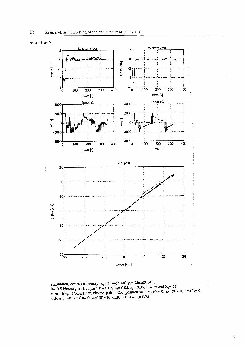
F: Results of the controlling of the end-effector of the xy table
situation 3 tr. error x-pos 2, i
- o Y
0 B
-6' I
O 100 200 300 400 time [-I
____..______._._____. -
.._. <............ > ...,............. $ ...............-
-6 ' o 100 200 300 400 time [-I
-40000 100 200 300 400 O 100 200 300 400 time [-I time [-I
e.e. path
8, x
x-pos [cm]
simulation, desired trajectory: xd= ~Ssin(3.14t) Yd= 25sin(3.14t), k= 0.5 Nm/rad, control gar.: k,= 0.05, k2= 0.05, k3= 0.05, hl= 25 and &= 25 meas. freq.: 1/0.01 Herz, obsew. poles: -25, position t=O: ~cp~(o)= o, ~%(o)= o, A d o ) = 0 velocity t=O: ~cp,(o)= O, ~rpl(O)= O, ~ip, (O)= O, a,= ay= 0.75
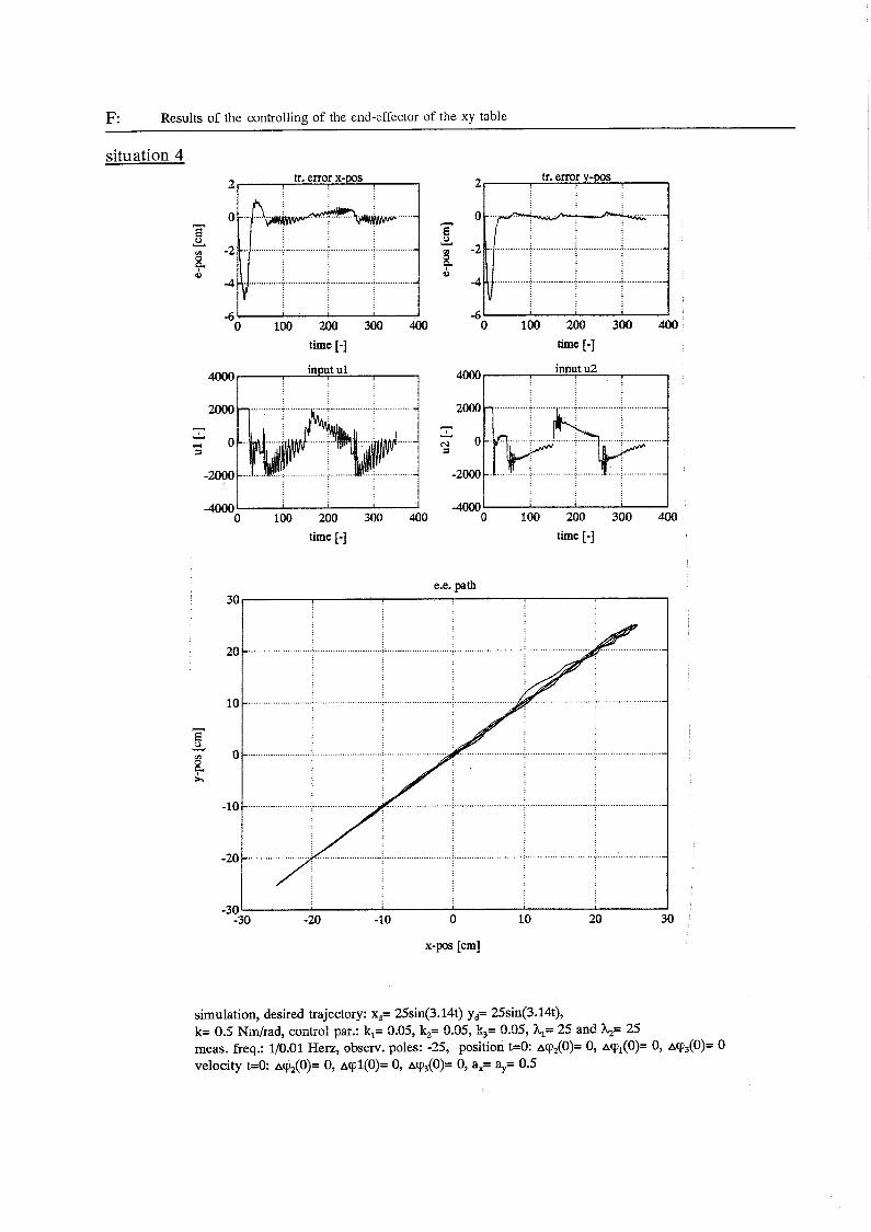
F: Results of the controlling of the end-effector of the xy table
situation 4 tr. error y-pos
I 2 tr. error x-pos 2 , I ..- -
.................. Y o 8
..........<.+.................i ...............-
j ...............- ................ e,
o 100 200 300 400 -6 o 100 200 300 400
time [-I time [-]
o 100 200 300 400 O 100 200 300 400 time [-I time [-I
e.e. path
simulation, desired trajectory: x,= 25sin(3.14t) yd= 25sin(3.14t), k= 0.5 Nm/rad, control par.: kl= 0.05, k2= 0.05, k,= 0.05, hl= 25 and &= 25 meas. freq.: 1/0.01 Herz, observ. poles: -25, position t=O: A ~ , ( O ) = O, ~ q p , ( O ) = O, ~rp,(O)= O velocity t=O: ~ c p , ( O ) = O, ~ c p l ( Q ) = O, ~ c p , ( O ) = O, a,= ay= 0.5
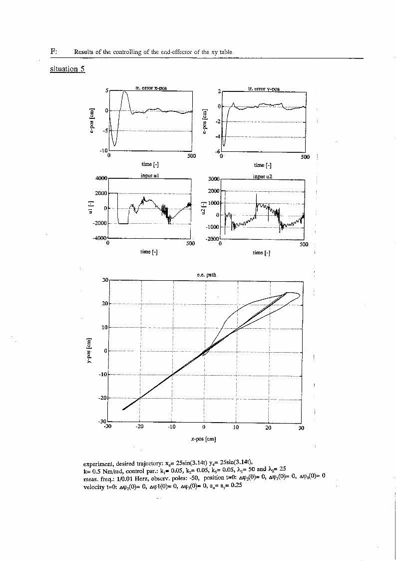
F: Results of the controlling of the end-effector of the xy table
- 0 E
I V I -10-
O 500
tr. error y-pos 2 1
8
-6 I I O 500
time [-I time [-I input u2 input u1
1 3000 4Ooo
...........................
I - 2 m - O 500 O 500
time [-I time [-]
e.e. uath
experiment, desired trajectory: xd= Zsin(3.14t) Yd= 25sin(3.14t), k= 0.5 Nm/rad, control par.: k,= 0.05, k,= 0.05, k,= 0.05, hl= 50 and &= 25 meas. freq.: 1/0.01 Herz, observ. poles: -50, position t=O acpZ(o)= o, A%(O)= 0, AT@)= 0 velocity t=O ~cp, (O)= O, ~cpl(O)= O, ~ c p , ( O ) = O, ax= ay= 0.25
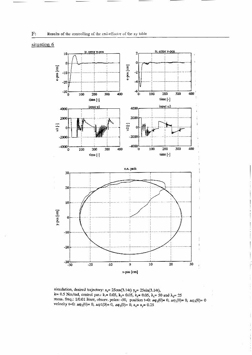
F: Results of the controlling of the end-effector of the xy table
situation 6
- E o
- Y
E o Y
u 8 0 8 -61 I 1
-30; 100 *00 3x0 400 o 100 200 300 400 time [-I time [-]
input u2 input u1 4000 4000
2000
F l 0 a
-2000
- Y
-4000 I -4000 ' J o 100 200 300 400 O 100 200 300 400 time [-] time [-I
x-pos [cm]
simulation, desired trajectory: xd= 25cos(3.14t) yd= 25sin(3.14t), k= 0.5 Nm/rad, control par.: k,= 0.05, k,= 0.05, k,= 0.05, hl= 50 and &= 25 meas. freq.: 1/0.01 Herz, observ. poles: -50, position t=O: ~ c p , ( O ) = O, ~ c p , ( O ) = O, acp,(O)= 0 velocity t=O: ~cp , (O)= O, ~cpl(O)= O, ~ c p , ( O ) = O, a,= ay= 0.25
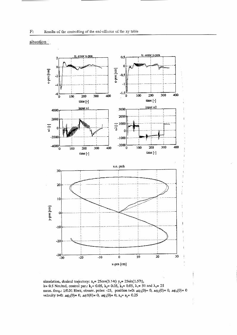
F: Results of the controlling of the end-effector of the xy table
situation, ,
- Y E3 - u 8
o Y
8 -.
o 100 200 300 400
time [-] time [-]
4Ooo
2000
* o
-2000
- Y
-40000 100 200 300 400 o 100 200 300 400 I'
time [-1 time [-]
e.e. path
.......... - -20 - ..........
-30 -20 -10 O 10 20 30
x-pos [cm]
-30
simulation, desired trajectory: xd= 25cos(3.14t) yd= 25sin( 1.57t), k= 0.5 Nm/rad, control par.: k,= 0.05, k2= 0.05, k,= 0.05, Al= 50 and &= 25 meas. freq.: 1/0.01 Herz, observ. poles: -25, position t=O: ~cp,(O)= O, acp1(O)= O, ~ c p ~ ( O ) = O velocity t=O: ~cp,(O)= O, ~ c p l ( O ) = O, ~ c p ~ ( O ) = O, ax= ay= 0.25
G. References
APPENDIX G: REFERENCES
Asada, H. and J. J. E. Slotine (1986) Robot analysis and control John Wiley Sons, New York
Oopov, V, M. (1969) Hyperstability of control systems Springer, New York
Slotine, J. J. E. and S . Hong (1987) Two-time scale sliding control of manipulators with flexible joints American Control Reference, pp. 805-810
Lammerts, I. M. M. (1991) Adaptive composite computed torque control of robots with elastic motor transmis- sions Aat,icle, Eindhoven University of Technology
Molengraft, M. J. 6. van de (1990) Identification of non-linear mechanical systems ISBN 90-9003596-6, Eindhoven University of Technology
Heeren, T. A. G. (1989) On control of manipulators ISBN 90-9002789-0, Eindhoven University of Technology
Kok, J. J. (1990) Regelen 2, Regelen 3, Regelen 4 Lecture notes, Eindhoven University of Technology
Kammer, R (1987) Numerieke methoden voor technici ISBN 90 6674 801 X
G. l.

![수치해석 (Numerical Analysis] · 2019. 8. 29. · 법 칙 (rule) 자연 ... xyy 2 xxxxy 6543 2 xyxyxyxyxy xy xy xy xy xy yxyyxyyxyy 65432 22 3 23 4 24 5623456 ... 근한 결과를](https://img.pdfslide.net/doc/110x75/6094b2bc38b4a6116148a9c8/-numerical-analysis-2019-8-29-e-rule-xyy-2.jpg)