Eindhoven University of Technology

MASTER

Investigation on the integration of a cross polarization interference canceller (XPIC)into a Nokia specific digital radio system

Driesen, B.

Award date:2001

DisclaimerThis document contains a student thesis (bachelor's or master's), as authored by a student at Eindhoven University of Technology. Studenttheses are made available in the TU/e repository upon obtaining the required degree. The grade received is not published on the documentas presented in the repository. The required complexity or quality of research of student theses may vary by program, and the requiredminimum study period may vary in duration.

General rightsCopyright and moral rights for the publications made accessible in the public portal are retained by the authors and/or other copyright ownersand it is a condition of accessing publications that users recognise and abide by the legal requirements associated with these rights.

• Users may download and print one copy of any publication from the public portal for the purpose of private study or research. • You may not further distribute the material or use it for any profit-making activity or commercial gain

Take down policyIf you believe that this document breaches copyright please contact us providing details, and we will remove access to the work immediatelyand investigate your claim.

Download date: 02. Jun. 2018

TECHNISCHE UNIVERSITEIT EINDHOVEN

FACULTEIT ELEKTROTECHNIEK

LEERSTOEL Signal Processing Systems

Investigation on the Integration ofa cross Polarization InterferenceCanceller (XPIC) into a Nokiaspecific Digital Radio System

B. Driesen

SPS 06-01

Verslag van een afstudeerproject verricht binnen deleerstoel Signal Processing Systems, oJ.v.prof.dr.ir. J.W.M. Bergmans en dr.ir. D. Gaschlerin de periode november 2000 - augustus 2001

Eindhoven, augustus 2001

De faculteit Elektrotechniek van de Technische Universiteit Eindhoven aanvaardt geenaansprakelijkheid voor de inhoud van dit verslag.

Investigation on the Integration of a Cross PolarizationInterference Canceller (XPIC) into a Nokia specific

Digital Radio System

by Bas Driesen

Preface

The compilation of this report is the result of my master thesis at the Department ofElectrical Engineering at the Eindhoven University of Technology. The empiricalresearch was done at and sponsored by Nokia Networks in DUsseldorf Germany. DuringNovember 15t 2000 to August 21 5t 2001 I have been working with the Radio Architectureand Integration Team of the System Competence Area. They have been great colleaguesand with some of them I spent some enjoyable moments after working-hours. Team,thanks for the nice atmosphere and for your support.

I would like to thank my supervisor, Prof. Dr. Ir. J.W.M. Bergmans of the SignalProcessing Systems Group in Eindhoven, for his useful critics and his cooperation. Iwould also like to thank my supervisor at Nokia, Dr. Ir. D. Gaschler of the RadioArchitecture and Integration Team, for the fruitful discussions and for being a greatsource of inspiration. I am grateful to the both of them for proofreading my manuscript,which enabled me to make it magnitudes better.

FUl1hermore I would like to thank my family for all their love, SUpp0l1 andencouragement. Finally I would like to express my gratitude to my dear girlfriend, for herpatience and understanding, especially in times when thoughts about the thesis controlledthe weekends.

Bas DriesenDUsseldorf, August 10th 2001

3

Abstract

Bandwidth efficiency of digital radio systems can be increased when the horizontal andvertical polarization of the antenna are used. All kind of factors can influence the degreeof orthogonality between the polarization directions, resulting in interference in eachdirection. To preserve receiver operation it is necessary to consider techniques that cancelthis interference. A Cross Polarization Interference Canceller (XPIC) is able to achievejust this.

Integrating an XPIC into an eXIstmg radio architecture involves dealing with manyproblems. This report deals with the interaction between XPIC, Automatic Gain Control(AGC), Adaptive Transversal Equalizer (ATE) and Phase Estimator (PE) under differentchannel assumptions. Additionally, timing differences between horizontally andvertically polarized receiver and frequency variations in the oscillators of the transmittersand receivers are studied.

Still, some remaining matters should be subjected to future research. Especially theinfluence of interference on the slow (non-decision aided) loops and the pilot detectionmodule should be investigated.

5

Table of Contents:

1. Introduction 9

2. Short Haul Digital Line-of-sight Radio Relay Systems 11

2.1 Nokia specific digital radio system 12

3. Fundamentals of adaptive filter theory 15

3.1 Wiener filters 153.2 Method of Steepest Decent 183.3 The Least-Mean-Square Algorithm 19

4. Cross Polarization Interference Canceller 23

4.1 Definitions 244.2 Functionality of the XPIC 244.3 XPIC Filter Structure 27

5. Simulations 31

5.1 XPIC Specific Simulations 315.1.1 System Considerations 315.1.2 Positioning the Decision Aided AGC 34

5.1.2.1 Problem Sketch 345.1.2.2 Simulation Outline 355.1.2.3 Simulation Results 355.1.2.4 Interpretation of the Simulation Results 41

5.1.3 Timing Sensitivity of the XPIC 415.1.3.1 Problem Sketch 415.1.3.2 Simulation Outline 425.1.3.3 Simulation Results 425.1.3.4 Interpretation of the Simulation Results 45

5.1.4 Frequency Offsets between the Oscillators of the Radio 465.1.4.1 Problem Sketch 465.1.4.2 Simulation Outline 475.1.4.3 Simulation Results 475.1.4.4 Interpretation of the Simulation Results 52

5.1.5 Phase Shifts in the Channel Paths 525.1.5.1 Problem Sketch 525.1.5.2 Simulation Outline 565.1.5.3 Simulation Results 575.1.5.4 Interpretation of the Simulation Results 59

5.2 System Performance Simulations 605.2.1 System Considerations 605.2.2 Flat Channel System Measurements 635.2.3 Multipath Channel System Measurements 63

6. Conclusions 65

7

7. Recommendations 67

8. List of Abbreviations 69

9. References 71

Appendix A: Timing Sensitivity Simulation Results 73

Appendix 8: Simulation Environment.. 77

8

1. Introduction

The increasing demand in voice and high-speed data traffic tends to provoke a saturationof the spectrum in digital radio systems, furthennore events such as spectral pricing aremore and more cornmon. These are two reasons for implementing systems with higherspectral efficiency. Efficient bandwidth utilization can be obtained by using high-levelmodulation techniques. Nowadays multilevel Quadrature Amplitude Modulation (QAM)and Trellis Coded Modulation (TCM) schemes are widely used.

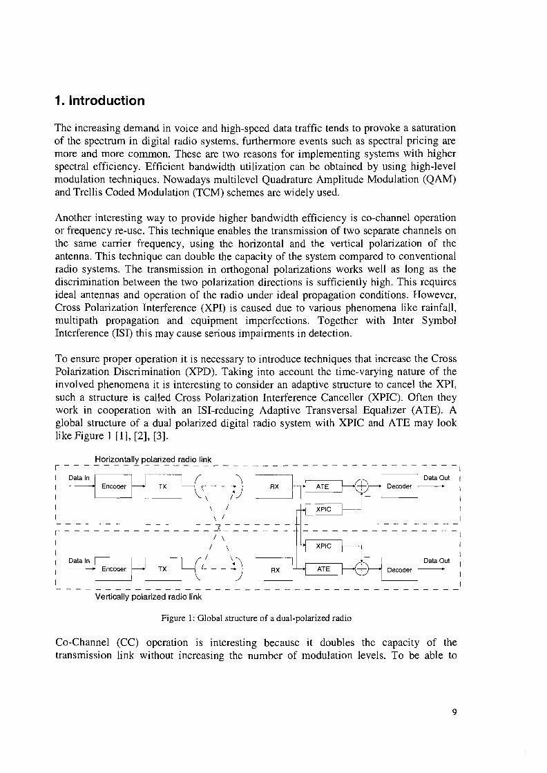
Another interesting way to provide higher bandwidth efficiency is co-channel operationor frequency re-use. This technique enables the transmission of two separate channels onthe same carrier frequency, using the horizontal and the vertical polarization of theantenna. This technique can double the capacity of the system compared to conventionalradio systems. The transmission in orthogonal polarizations works well as long as thediscrimination between the two polarization directions is sufficiently high. This requiresideal antennas and operation of the radio under ideal propagation conditions. However,Cross Polarization Interference (XPI) is caused due to various phenomena like rainfall,multipath propagation and equipment imperfections. Together with Inter SymbolInterference (lSI) this may cause serious impainnents in detection.

To ensure proper operation it is necessary to introduce techniques that increase the CrossPolarization Discrimination (XPD). Taking into account the time-varying nature of theinvolved phenomena it is interesting to consider an adaptive structure to cancel the XPI,such a structure is called Cross Polarization Interference Canceller (XPIC). Often theywork in cooperation with an lSI-reducing Adaptive Transversal Equalizer (ATE). Aglobal structure of a dual polarized digital radio system with XPIC and ATE may looklike Figure 1 [1], [2], [3].

Horizontally polarized radio link,----------------------------------------1

I ~ H 'K )---c:J Data Out II -l Encoder I TX \" - - -: RX \

I \ / I

I \ / I

I \ / I

~~~~~~~~~~~~~~~~~~~~~~~~/ \

I /

:~ H K/ \.I I Encoder TX L - - -

I

Vertically polarized radio link

Figure 1: Global structure of a dual-polarized radio

Co-Channel (CC) operation is interesting because it doubles the capacity of thetransmission link without increasing the number of modulation levels. To be able to

9

achieve comparable performance (bit enol' rate) for co-channel systems as for singlepolarized radio systems an XPIC needs to be introduced in the receiver.

The XPIC is a well-known subject in literature, with lot of discussions devoted to it.Especially upgrading the available single polarized radio to a dual polarized radio hasbeen a major issue. The main reason for this is that the product can be sold as a singlepolarized radio system when less capacity is needed and as a dual polarized radio systemwhen more capacity is needed. Allowing the customer to buy a single polarized radiosystem first and maybe upgrading it to a dual polarized radio system in the future.Operation of a dual polarized radio system comprises of two interconnected radios, thismeans that the single polarized radio system needs to be compatible with the dualpolarized radio system. Just like other manufacturers Nokia is interested in upgrading itsradio system. However there are of course some differences between the Nokia radiosystem and the radio systems described in the literature.

In this study the integration of an XPIC into a Nokia specific digital radio system isinvestigated. Interactions between XPIC, Automatic Gain Control (AGC), PhaseEstimator (PE) as well as the ATE are studied. Furthermore the XPIC's performance andthe system's performance are measured under different channel conditions and equipmentimperfections.

First the Nokia specific digital radio system is explained in Chapter 2. After that somefundamentals of adaptive filter theory are recalled in Chapter 3, necessary for a deeperunderstanding of the XPIC. Then Chapter 4 elaborates on the XPIC and a basicsimulation model is derived. Chapter 5 treats the studied aspects as mentioned in theformer paragraph on the basis of simulations, verified by theoretical analyses.Additionally, it provides an overview of the corresponding findings in the literature.Finally Chapter 6 and Chapter 7 give the conclusions and the recommendations of thisstudy.

10

2. Short Haul Digital Line-of-sight Radio Relay Systems

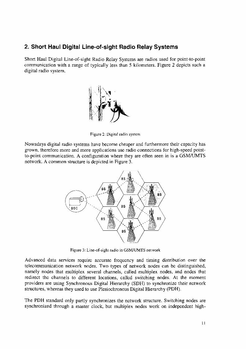
Short Haul Digital Line-of-sight Radio Relay Systems are radios used for point-to-pointcommunication with a range of typically less than 5 kilometers. Figure 2 depicts such adigital radio system.

Figure 2: Digital radio system

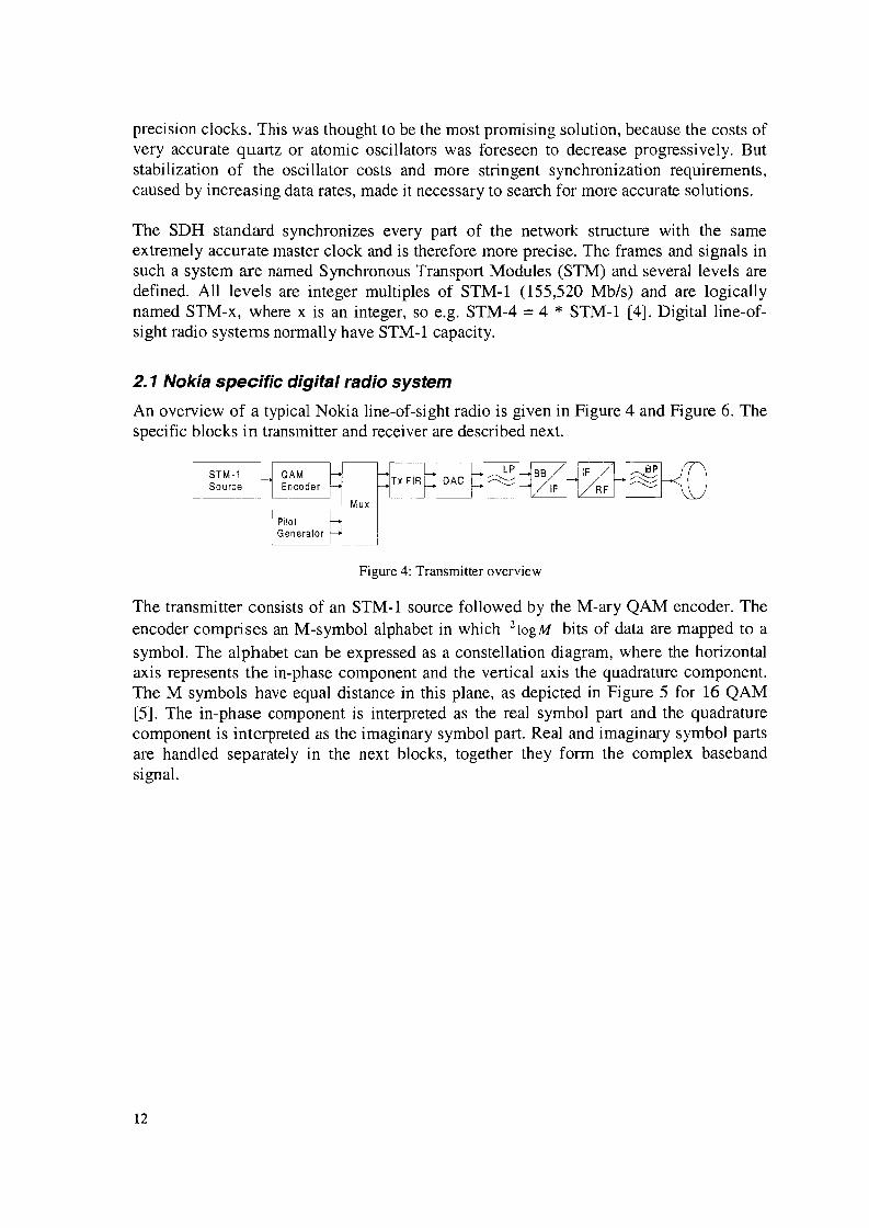
Nowadays digital radio systems have become cheaper and furthermore their capacity hasgrown, therefore more and more applications use radio connections for high-speed point­to-point communication. A configuration where they are often seen in is a GSM/UMTSnetwork. A common structure is depicted in Figure 3.

Figure 3: Line-of-sight radio in GSMlUMTS network

Advanced data services require accurate frequency and timing distribution over thetelecommunication network nodes. Two types of network nodes can be distinguished,namely nodes that multiplex several channels, called multiplex nodes, and nodes thatredirect the channels to different locations, called switching nodes. At the momentproviders are using Synchronous Digital Hierarchy (SDH) to synchronize their networkstructures, whereas they used to use Plesiochronous Digital Hierarchy (PDH).

The PDH standard only partly synchronizes the network structure. Switching nodes aresynchronized through a master clock, but multiplex nodes work on independent high-

11

precision clocks. This was thought to be the most promising solution, because the costs ofvery accurate quartz or atomic oscillators was foreseen to decrease progressively. Butstabilization of the oscillator costs and more stringent synchronization requirements,caused by increasing data rates, made it necessary to search for more accurate solutions.

The SDH standard synchronizes every part of the network structure with the sameextremely accurate master clock and is therefore more precise. The frames and signals insuch a system are named Synchronous Transport Modules (STM) and several levels aredefined. All levels are integer multiples of STM-1 (155,520 Mb/s) and are logicallynamed STM-x, where x is an integer, so e.g. STM-4 =4 * STM-1 [4]. Digital line-of­sight radio systems normally have STM-1 capacity.

2.1 Nokia specific digital radio system

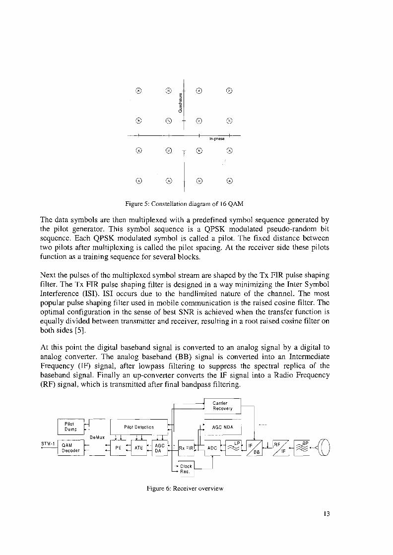
An overview of a typical Nokia line-of-sight radio is given in Figure 4 and Figure 6. Thespecific blocks in transmitter and receiver are described next.

~PBB ~FBP

TxFIR DAC ~ ~IF RF

Figure 4: Transmitter overview

The transmitter consists of an STM-1 source followed by the M-ary QAM encoder. Theencoder comprises an M-symbol alphabet in which 2 10gM bits of data are mapped to a

symbol. The alphabet can be expressed as a constellation diagram, where the horizontalaxis represents the in-phase component and the vertical axis the quadrature component.The M symbols have equal distance in this plane, as depicted in Figure 5 for 16 QAM[5]. The in-phase component is interpreted as the real symbol part and the quadraturecomponent is interpreted as the imaginary symbol part. Real and imaginary symbol partsare handled separately in the next blocks, together they form the complex basebandsignal.

12

0 0I

0

~r0

lii~:00

0 8 (') 0

In-phase

0 @ 0 0

o o o o

Figure 5: Constellation diagram of 16 QAM

The data symbols are then multiplexed with a predefined symbol sequence generated bythe pilot generator. This symbol sequence is a QPSK modulated pseudo-random bitsequence. Each QPSK modulated symbol is called a pilot. The fixed distance betweentwo pilots after multiplexing is called the pilot spacing. At the receiver side these pilotsfunction as a training sequence for several blocks.

Next the pulses of the multiplexed symbol stream are shaped by the Tx FIR pulse shapingfilter. The Tx FIR pulse shaping filter is designed in a way minimizing the Inter SymbolInterference (lSI). lSI occurs due to the bandlimited nature of the channel. The mostpopular pulse shaping filter used in mobile communication is the raised cosine filter. Theoptimal configuration in the sense of best SNR is achieved when the transfer function isequally divided between transmitter and receiver, resulting in a root raised cosine filter onboth sides [5].

At this point the digital baseband signal is converted to an analog signal by a digital toanalog converter. The analog baseband (BB) signal is converted into an IntermediateFrequency (IF) signal, after lowpass filtering to suppress the spectral replica of thebaseband signal. Finally an up-converter converts the IF signal into a Radio Frequency(RF) signal, which is transmitted after final bandpass filtering.

Figure 6: Receiver overview

13

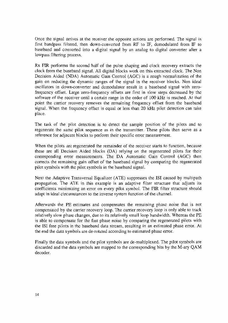
Once the signal anives at the receiver the opposite actions are performed. The signal isfirst bandpass filtered, then down-converted from RF to IF, demodulated from IF tobaseband and converted into a digital signal by an analog to digital converter after alowpass filtering process.

Rx FIR performs the second half of the pulse shaping and clock recovery extracts theclock from the baseband signal. All digital blocks work on this extracted clock. The NonDecision Aided (NDA) Automatic Gain Control (AGC) is a rough normalization of thegain on reducing the dynamic ranges of the signal in the receiver blocks. Non idealoscillators in down-converter and demodulator result in a baseband signal with zero­frequency offset. Large zero-frequency offsets are first in slow steps decreased by thesoftware of the receiver until a certain range in the order of 100 kHz is reached. At thatpoint the camer recovery removes the remaining frequency offset from the basebandsignal. When the frequency offset is equal or less than 20 kHz pilot detection can takeplace.

The task of the pilot detection is to detect the sample positIon of the pilots and toregenerate the same pilot sequence as in the transmitter. These pilots then serve as areference for adjacent blocks to perform their specific error measurement.

When the pilots are regenerated the remainder of the receiver starts to function, becausethese are all Decision Aided blocks (DA) relying on the regenerated pilots for theircorresponding error measurements. The DA Automatic Gain Control (AGC) thencorrects the remaining gain offset of the baseband signal by comparing the regeneratedpilot symbols with the pilot symbols in the baseband signal.

Next the Adapti ve Transversal Equalizer (ATE) suppresses the lSI caused by multipathpropagation. The ATE in this example is an adaptive filter structure that adjusts itscoefficients minimizing an error on every pilot symbol. The FIR filter structure shouldadapt in ideal circumstances to the inverse system function of the channel.

Afterwards the PE estimates and compensates the remaining phase noise that is notcompensated by the carrier recovery loop. The carrier recovery loop is only able to trackrelatively slow phase changes, due to its relatively small loop bandwidth. Whereas the PEis able to compensate for the fast phase noise by comparing the regenerated pilots withthe lSI free pilots in the baseband data stream, resulting in an estimated phase error. Atthe end the data symbols are de-rotated according to estimated phase error.

Finally the data symbols and the pilot symbols are de-multiplexed. The pilot symbols arediscarded and the data symbols are mapped to the corresponding bits by the M-ary QAMdecoder.

14

3. Fundamentals of adaptive filter theory

This Chapter recalls some well-known concepts from the Wiener filter theory and leadsto Least Mean Square (LMS) algorithm used by the XPIC.

3. 1 Wiener filters

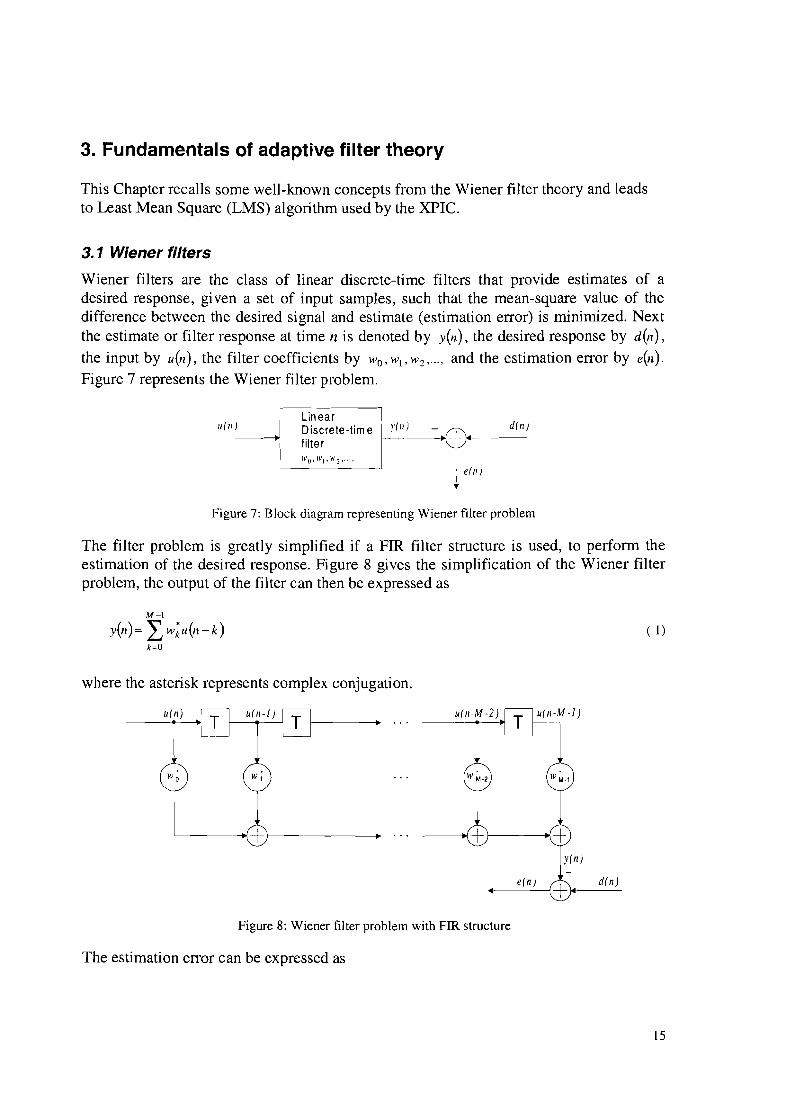
Wiener filters are the class of linear discrete-time filters that provide estimates of adesired response, given a set of input samples, such that the mean-square value of thedifference between the desired signal and estimate (estimation error) is minimized. Nextthe estimate or filter response at time n is denoted by y(n) , the desired response by d01),the input by u(n), the filter coefficients by Wo, WI' Wz , ... , and the estimation error by e0t).Figure 7 represents the Wiener filter problem.

U(II)Lin ea rDiscrete-time y(n) d(n)filte r I-------.{+~---

"'0> WI' ""2.···'

I e(n)...

Figure 7: Block diagram representing Wiener filter problem

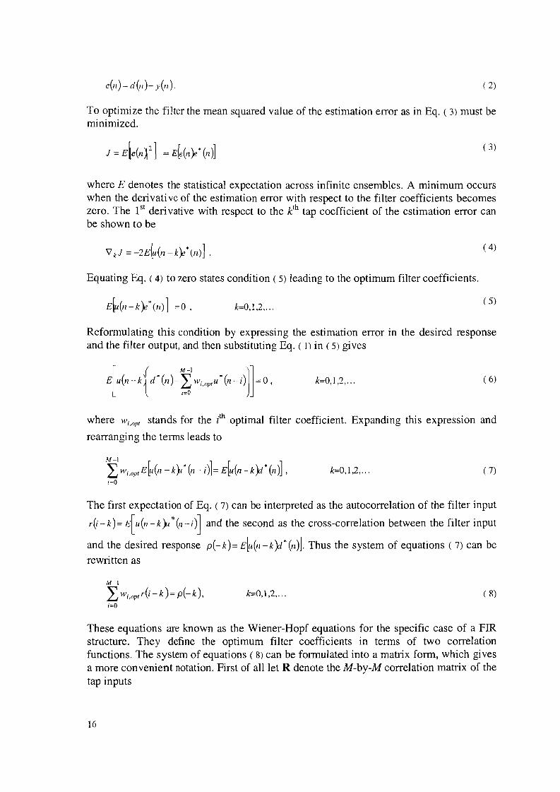
The filter problem is greatly simplified if a FIR filter structure is used, to perform theestimation of the desired response. Figure 8 gives the simplification of the Wiener filterproblem, the output of the filter can then be expressed as

M-I

y(n)== L w;u0t-k)k=O

where the asterisk represents complex conjugation.

urn)

'-----------.l+f----------_

Figure 8: Wiener filter problem with FIR structure

The estimation error can be expressed as

din)

( 1)

15

e(n)== d(II)- y(n). ( 2)

To optimize the filter the mean squared value of the estimation error as in Eq. ( 3) must beminimized.

( 3)

where E denotes the statistical expectation across infinite ensembles. A minimum occurswhen the derivative of the estimation error with respect to the filter coefficients becomeszero. The 1st derivative with respect to the kth tap coefficient of the estimation error canbe shown to be

Equating Eq. (4) to zero states condition (5) leading to the optimum filter coefficients.

( 4)

k==O,1,2, ...( 5)

Reformulating this condition by expressing the estimation error in the desired responseand the filter output, and then substituting Eq. ( 1) in ( 5) gives

k==0,1,2, ... ( 6)

where W i •opt stands for the i th optimal filter coefficient. Expanding this expression and

rearranging the tenns leads to

M-l

L wi-opt e[U(1I - k~ •(II - i )]== E[u(n - k)d' (II)] ,;=0

k=O,1,2, ... ( 7)

The first expectation of Eq. ( 7) can be interpreted as the autocorrelation of the filter input

r(i-k)==E[lt(lI-k~*01-i)J and the second as the cross-correlation between the filter input

and the desired response p(-k)= E~l(ll-k)d·(Il)J.Thus the system of equations ( 7) can berewritten as

M-l

L wi,optr(i - k)= p(-k),;=0

k=O,1,2, ... ( 8)

These equations are known as the Wiener-Ropf equations for the specific case of a FIRstructure. They define the optimum filter coefficients in terms of two correlationfunctions. The system of equations ( 8) can be formulated into a matrix form, which givesa more convenient notation. First of all let R denote the M-by-M correlation matrix of thetap inputs

16

1'(0) r(l) r(M -1)I' * (1) 1'(0) r(M -2)

R = E[U(npH (n)]=( 9)

1'* (M -1) ,.. (M -2) r(O)

where u(n)denotes the M-by-l tap-input vector, defined as

( 10)

the superscript T stands for the transposition operation and the superscript H stands forthe Hennitian adjoint or the conjugated transposed. Second let p denote the M-by-lcross-correlation vector between the tap-inputs and the desired response

( 11)

Now the Wiener-Hopf equations can be rewritten in the compact matrix notation fonn:

RW apt =e,

where w opt denotes the M-by-l optimum tap-weight vector defined as

W opt = [wopt,o, wopt,1 , .. " wopt,M-1 f .

( 12)

( 13)

Premultiplying both sides with the inverse of the autocorrelation matrix R"l assuming thatthe autocorrelation matrix R is nonsingular will lead to the solution to the Wiener-Hopfequations

R - 1Wapt = e· ( 14)

For the computation of the optimum tap-weights the autocorrelation matrix R and thecross-correlation vector p must be known. Solving the Wiener-Hopf equations directlyrequires a lot of computational power and presents therefore serious difficulties,especially when the filter consist of a large number of tap weights and when the inputdata rate is high. In the next subchapter the method of steepest decent is described; analternative procedure for computing the optimal filter coefficients in a recursive fashion.That is calculating the tap-weights starting from an initial value and improving ititeratively. Eventually the values will converge to the Wiener-Hopf solution [6].

When studying a filter problem it is useful to have a simple expression for the minimumof the mean squared error. Inserting the optimum tap-weights into Eg. ( 1) results in anoptimal filter output

17

( 15)

When the linear discrete-time filter in Figure 8 operates In optimum condition theestimation error takes on the following form

( 16)

The minimum mean squared error is then defined by

Substituting Eq. ( 16) into Eq. ( 17) and using Eq. ( 15) and Eq. ( 14) leads to

J 2 H R-1min =(J'd-Q Q.

( 17)

( 18)

This definition shows the minimum mean squared error in terms of the variance of thedesired response (J'~, the autocon'elation matrix R and the cross-correlation vector p [6].

3.2 Method of Steepest Decent

The method of steepest decent is an optimization technique that is based on gradientadaptation. The gradient derived in the previous chapter can be written in the followingmatrix notation

VJ(n) = -2Q + 2Rw(n)

where VJ(n) is the M-by-l gradient vector defined by

and in which w(n) is the instantaneous tap-weight vector at time 11 defined by

( 19)

( 20)

( 21)

It can be shown that the mean squared estimation error J of Eq. ( 3) is a squared functionof the tap-weights. The mean squared estimation error can therefore be seen as a multi­dimensional parabolic-shaped surface with respect to the tap-weights. A property of aparabola is that its gradient always points away from its minimum. The method ofsteepest decent uses this information in a recursive way. Adding a small fraction of thenegative error gradient to the old tap-weight vector forms a new tap-weight vector.Proceeding in an iterative way will finally result into the optimal filter coefficients.Accordingly the updated value of the tap-weight vector at time 11 +1, the tap-weightvector at time 11 and the mean squared error gradient vector at time 11 form the recursiverelation

18

w(n +1)= w(n)+ ~ j.L[- VJ(n)]2 ( 22)

where 1.L is called the step-size parameter and is a positive real-valued constant. The factorYz is used merely to cancel the factor 2 in the error gradient. Now substituting Eq. ( 19) in( 22) gives the final form of the update algorithm [6]

11=0,1,2, ... ( 23)

3.3 The Least-Mean-Square Algorithm

The Least-Mean-Square (LMS) algorithm differs form the method of steepest decent, itdoes not compute the actual mean squared error gradient vector, but it calculates aninstantaneous estimate of this vector. The big advantage is that this does not require anyprior knowledge about the correlation matrix R of the tap inputs and the cross-correlationvector p of the tap inputs and the desired response. However the drawback of thisalgorithm is that the tap-weights approach the Wiener solution, but will never exactlyreach it. In general there will be always a random motion around the minimum of theestimation error surface, causing a misadjustment. This means the final value of themean-squared error J consist of the minimum mean squared error JlIlin plus an excessmean squared error Jex, due to the instantaneous estimate of the gradient vector. When theexpectation operation in the gradient vector of Eq. ( 4) is left out, it will result in theinstantaneous estimate of the gradient vector

VJ(Il) =-2u(Il)d' (Il)+ 2u(ll:UH(Il)w(Il) ( 24)

where " indicates an estimate. Using this gradient estimate in the steepest decentalgorithm described in Eq. ( 22) rises a new recursive relation for updating the filtercoefficients:

( 25)

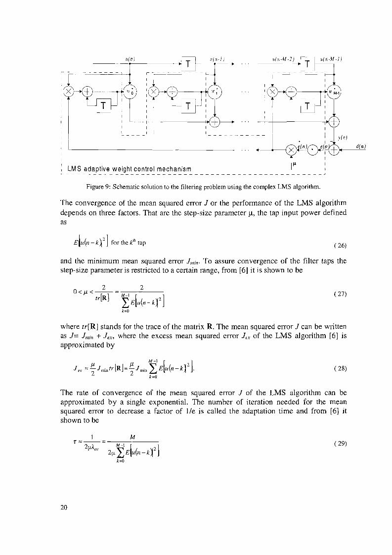
The LMS filter algorithm involves two processes, namely a filtering process thatcomputes the filter output and an adaptive process that automatically adjusts the tapweights. The last one is called the adaptive weight-control mechanism. Figure 9 shows aschematic solution to the filtering problem making use of the complex LMS algorithm[6].

19

din)

-. ...ul 11- J)

, - - - - - - - - - - L--

I I II

_______U...II1_) --11LL

LMS adaptive weight control mechanism_________________________________________________ J

: :I ---t+i+I:T I Ie-- I-_-_-_-_-_'_I I - - - - - - - - - .-.-_--.J---tl~__{ X

Figure 9: Schematic solution to the filtering problem using the complex LMS algorithm.

The convergence of the mean squared error 1 or the performance of the LMS algorithmdepends on three factors. That are the step-size parameter j!, the tap input power definedas

( 26)

and the minimum mean squared error lllli/!. To assure convergence of the filter taps thestep-size parameter is restricted to a certain range, from [6] it is shown to be

2 20<j.1.<--=------

tr[R] YEiu(n-q2]k=O

( 27)

where tr[R] stands for the trace of the matrix R. The mean squared error 1 can be writtenas l= lmill + lex, where the excess mean squared error lex of the LMS algorithm [6] isapproximated by

( 28)

The rate of convergence of the mean squared error 1 of the LMS algorithm can beapproximated by a single exponential. The number of iteration needed for the meansquared error to decrease a factor of lie is called the adaptation time and from [6] itshown to be

1 Mr ""--= --.,.------

2fJ)'av ~l f ( ,/2]2f-l..LiE~u n-k-1

k=O

( 29)

20

where fl is the step-size parameter and Aav IS the average of the eigenvalues of thecorrelation matrix R.

21

4. Cross Polarization Interference Canceller

The capacity of radio systems can be doubled when operating in co-channel mode. Thistechnique enables the transmission of two separate channels on the same carrierfrequency, using the horizontal and the vertical polarization of the antenna. Thetransmission in orthogonal polarizations works well as long as the discriminationbetween the two polarization directions is sufficiently high. This demands operation ofthe radio under near-ideal propagation conditions. However, Cross-PolarizationInterference (XPI) is caused due to various phenomena like rainfall, multipathpropagation and equipment imperfections. To ensure operation it is necessary tointroduce techniques that increase the Cross-Polarization Discrimination (XPD),especially when high-level modulation schemes are in use. This is accomplished with anadaptive filter that is able to take into account the time-varying nature of the involvedphenomena. Such a structure is called Cross Polarization Interference Canceller (XPIC).

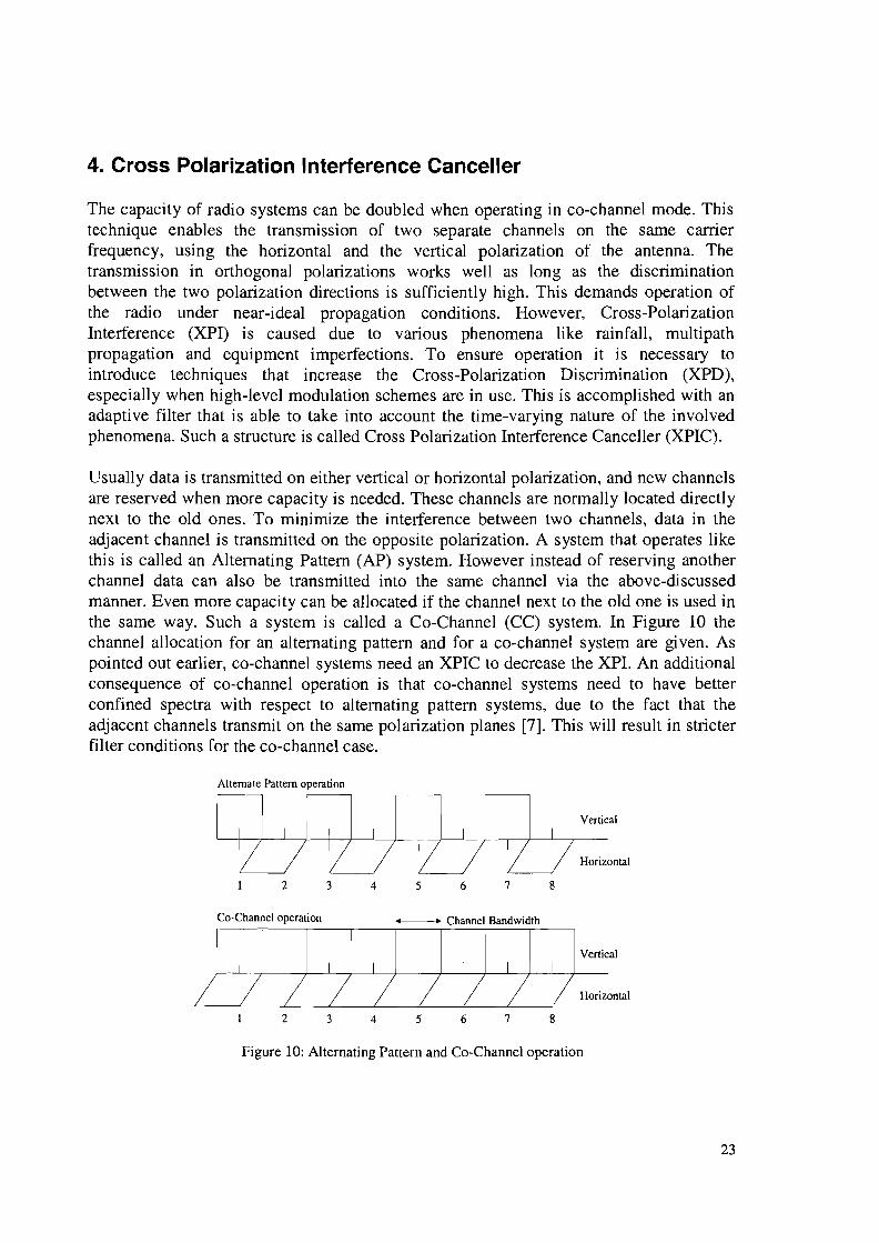
Usually data is transmitted on either vertical or horizontal polarization, and new channelsare reserved when more capacity is needed. These channels are normally located directlynext to the old ones. To minimize the interference between two channels, data in theadjacent channel is transmitted on the opposite polarization. A system that operates likethis is called an Alternating Pattern (AP) system. However instead of reserving anotherchannel data can also be transmitted into the same channel via the above-discussedmanner. Even more capacity can be allocated if the channel next to the old one is used inthe same way. Such a system is called a Co-Channel (CC) system. In Figure 10 thechannel allocation for an alternating pattern and for a co-channel system are given. Aspointed out earlier, co-channel systems need an XPIC to decrease the XPI. An additionalconsequence of co-channel operation is that co-channel systems need to have betterconfined spectra with respect to alternating pattern systems, due to the fact that theadjacent channels transmit on the same polarization planes [7]. This will result in stricterfilter conditions for the co-channel case.

Alternate Pattern operation

Vertical

Horizontal

2 3 4 5 6 7 8

65432

Co-Channel operation __ Channel Bandwidth

fttllH ~:ml7 8

Figure 10: Alternating Pattern and Co-Channel operation

23

4. 1 Definitions

The XPI and the XPD are two important parameters related to the XPIC, their definitionsare given by:

XPI = 20log II

EIffiII [dB]

EYH

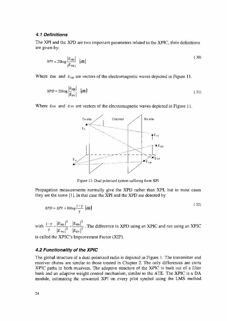
Where EHH and E YH are vectors of the electromagnetic waves depicted in Figure 11.

Where EHH and E HV are vectors of the electromagnetic waves depicted in Figure 11.

( 30)

( 31)

Tx-site

Evr<:::~---~::::::

Channel

........_----...

Rx-site

Figure 11: Dual polarized system suffering form XPI

Propagation measurements normally give the XPD rather than XPI, but in most casesthey are the same [1]. In that case the XPI and the XPD are denoted by

XPD = XPI = lOlog l-y [dB]Y

( 32)

with 1- y = IEHH I: = [EHH I: .The difference in XPD using an XPIC and not using an XPICy IEYH I IEHv l-

is called the XPIC's Improvement Factor (XIF).

4.2 Functionality of the XPIC

The global structure of a dual-polarized radio is depicted in Figure 1. The transmitter andreceiver chains are similar to those treated in Chapter 2. The only differences are extraXPIC paths in both receivers. The adaptive structure of the XPIC is built out of a filterbank and an adaptive weight control mechanism, similar to the ATE. The XPIC is aDAmodule, estimating the unwanted XPI on every pilot symbol using the LMS method

24

described in Chapter 3. It correlates the differently polarized signals in the receiver. Anessential detail then is the uniqueness of horizontal and vertical sources. Although thesources may be identical when instead of a QAM scheme a TCM scheme is used. Aprerequisite then is the use of different scramblers for each polarization [8].

Furthermore from the literature [9] it is shown that when the filter lengths of the XPICand ATE are equal, the XPIC can be placed preceding the ATE, can be placed parallel tothe ATE or the ATE can be placed preceding the XPIC. When the filters have differentspans it is a disadvantage to place the longer filter in front of the shorter one, since it cancause far echoes due to their individual tap weighting [9]. The shorter filter is than notable to exercise control over the extra taps of the longer filter. Because of a less complexcircuitry the parallel variant is chosen.

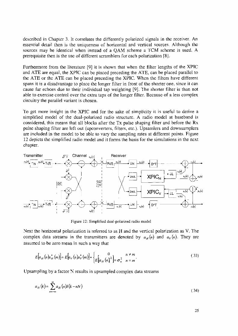
To get more insight in the XPIC and for the sake of simplicity it is useful to derive asimplified model of the dual-polarized radio structure. A radio model at baseband isconsidered, this means that all blocks after the Tx pulse shaping filter and before the Rxpulse shaping filter are left out (upconverters, filters, etc.). Upsamlers and downsamplersare included in the model to be able to vary the sampling rates at different points. Figure12 depicts the simplified radio model and it forms the basis for the simulations in the nextchapter.

III

I

I

'ciDi

IT/N '1--1II

I :

~Figure 12: Simplified dual-polarized radio model

1-----41+ ,,,(II

I-----~+ zvH

Next the horizontal polarization is referred to as H and the vertical polarization as V. Thecomplex data streams in the transmitters are denoted by aH 01) and av(n). They areassumed to be zero mean in such a way that

n:Fm

n=m

( 33)

Upsampling by a factor N results in upsampled complex data streams

~

aH(k)= ~>H (n)5(k -nN)( 34)

25

~

ay(k)= Lay (n)5(k-IIN).n=-oo

The overall transfer function of the pulse shaping filters and the channel Q(e jQNT') can bedenoted in matrix form as

( 35)

where Tx (e jQNT') and RJe jQNT

') are the time-discrete root raised cosine frequency

responses ~N(ejQNT') of the pulse shaping filter, with T=T / N. The matrix C(Q)

represents the dually polarized propagation channel, in which C HH (n) and Cw (n) are the

co-polar responses and cYH (n) and cHY (n) are the unwanted cross-polar responses. Thesignal after the receiver's pulse shaping filter can be written as

II H(k) = L [a H01)q HH (k - IIN)+ ay (II )qYH (k - liN)J+ vH(k)n

n

( 36)

where qij (k) is the inverse time-discrete Fourier transform of the ith/lh element of the

overall transfer function Q(e jQNT'). v H (k) and V y (k) are two independent noise processes,

generated by filtering and sampling the two independent noise processes " H (t) and lI y (t)at the receiver [3]. When the channel is assumed to be flat and if only the depolarizationeffects are considered, Eq. ( 36) can be rewritten after downsampling with a factor N as

It H(kN) = It H(/1) =Jl- yaH (/1)+ f(ay (/1)+VH(/1)

ltv (kN) = ltv (11)= hay (/1)+f(a H(11)+V y (/1).

( 37)

The amount of XPI in the horizontal and vertical polarization is as[;umed to be equal,where the parameter y is a measure for the XPD.

If the input signals of the XPICs are also downsampled with a factor N (L=l), then thehorizontal baseband signal in Eq. ( 37) serves as input for the XPIC in the vertical radiolink and the vertical baseband signal in Eq. ( 37) serves as input for the XPIC in thehorizontal radio link. For now the AGCs and PEs are left out. The ATEs are redundantbecause the channel does not suffer from any multipath fading at this point. Both ATEsare replaced by a delay of D symbols, enabling the center tap of the XPIC's filter bank tobe configured.

The outputs of the XPICs must compensate the unwanted XPI signals. When an XPICfilter length of M is chosen, the outputs can be written in a similar form as Eq. ( 15)

26

yv (n)= wZv (n).IH (n). ( 38)

In which WVH (n)and W HV (n) are the M-by-l instantaneous tap-weight vectors ofrespectively the horizontal XPIC and the vertical XPIC at time n defined by Eq. ( 21), andUv (n) and UH (n) are the M-by-l tap-input vectors of respectively the horizontal XPIC andthe vertical XPIC at time n defined by Eq. ( 10). These outputs are then subtracted fromthe delayed baseband signals to form the corrected signals

ZH (n) = uH(11- D)- W ~H (n).Iv (11)

Zv (n) = Uv (n - D)- W Zv (n).I H(n).

( 39)

Subtracting the regenerated pilot signals from the corrected signals gives the estimationerror in the horizontal and vertical branches:

eH (11)= ZH (n)- PH (11)= ZH (11)-a H(n-D)

ev (n) = Zv (n)- Pv (n) = Zv Vl)- av (n - D).

They can be expressed in a similar fonTI as treated in Chapter 3, that is

eHVI) =UH(n - D)- aHVl- D)- YH(n) = d HVI)- YH(11)

ev Vl)= Uv VI- D)-av VI-D)- Yv (n)= dv (n)- Yv VI)

where d H (n) and dv(n) represent the desired responses for the XPICs.

( 40)

( 41)

4.3 XPIC Filter Structure

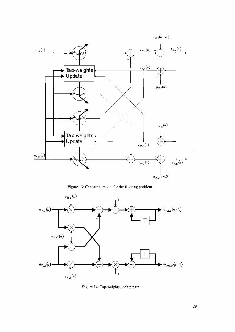
The algorithm behind the adaptive XPIC structure is the complex LMS algorithm.However the realization of this algorithm is a bit different than presented in Chapter 3.Instead of having single complex signals, the signals consist of two parts: a real partnamed the in-phase component and an imaginary part named quadrature component. Thisleads to the following notation for the data and tap-weights for the horizontal receiverbranch

Tap-input vector: Uv (n)= Uv,/ (n)+ jUV,Q(n) ( 42)

Regenerated pilots: PH (n)= PH'! (n)+ jPH,Q (11) ( 43)

Tap-weight vector: WVH (n)= WVH,l (n)+ jWvH,Q (n) ( 44)

Transversal filter output: YHVI) = YH,l VI) + jyH,Q (n) ( 45)

Corrected signal: ZH (n)= ZH,lVI)+ jZH,Q(n) ( 46)

Estimation error: eH (n) =eH,/ (n)+ jeH,Q (n) ( 47)

27

where I and Q stand for the in-phase and quadrature component respectively. Using thesedefinitions in the expressions of: the filter output Eq. ( 38), the estimation error Eq. ( 2),

the update relation Eq. (25) and the corrected signal Eq. ( 39) gives:

Filter output (in-phase): () ~ T (\. () ~ T (\. ()YH,I n = WVH,I npV,l n -WVH.Q npV.Q n

Filter output (quadrature): () ~ T (\. () ~ T (\. ()YH.Q n =WVH,I npv,Q n +wQ npV,I n

Corrected signal (in-phase): ZH,I (n) = uH,I (n - D)- YH,I (n)

Corrected signal (quadrature): ZH ,Q &1)= u H.Q (n - D)- YH.Q (n)

Estimation error (in-phase): eH,I &1) = ZH,I (n)- PH,I (n)

Estimation error (quadrature): ell.Q (n) = ZH.Q &1)- PH.Q &1)

( 48)

( 49)

( 50)

( 51)

( 52)

( 53)

Update relation (in-phase): ~ ( 1) ~ () r (\. () (\. ()] (54)WVH,I Il+ =W VH .1 n +f1LeH,I Ilpv,l n -eH.Q npv.Q II

Update relation (quadrature): ~ (1) ~ () r (\. () (\. ()] (55)WVH,Q n+ =WVH,Q n +f1LeH,I npv.Q II +eH.Q npv./ II

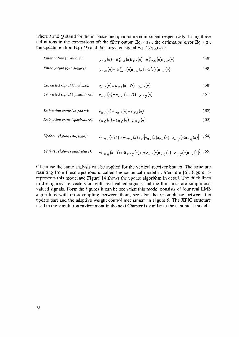
Of course the same analysis can be applied for the vertical receiver branch. The structureresulting from these equations is called the canonical model in literature [6]. Figure 13represents this model and Figure 14 shows the update algorithm in detail. The thick linesin the figures are vectors or multi real valued signals and the thin lines are simple realvalued signals. Form the figures it can be seen that this model consists of four real LMSalgorithms with cross coupling between them, see also the resemblance between theupdate part and the adaptive weight control mechanism in Figure 9. The XPIC structureused in the simulation environment in the next Chapter is similar to the canonical model.

28

"V.l (n)!f-------~+ f------~

eH.Jn)Ta p-weights 14--------+-~-_______ir--+----+I Update

/Ta p-weightst---...... Update 14---------1----+------) +'14--------,

eH.Q(n)

J)-----------.{+ - +j----+--

YH.Q(n) ZH.Q(n)

Figure 13: Canonical model for the filtering problem.

Figure 14: Tap-weights update part

29

5. Simulations

In the following Chapter a Synopsis tool named CoCentric System Studio is used forsimulation purposes. CoCentric System Studio is a system-level design suite consisting oftools, methodologies, and libraries that enables the design and simulation of systems-on­a-chip. System Studio provides several types of model implementations. The Data FlowGraph (DFG) is most suitable for creating the XPIC environment. A dataflow model is amodel in which the instances it contains communicate by means of FIFO (first in, firstout) queues of data travelling on the nets. The model schematic is graphically representedas a block diagram in which the modules can be ordered hierarchically. System Studioalready contains a wide selection of standard modules that can be instantiated into thedesign. This prevents writing all building blocks manually and therefore allows fastoperation. The XPIC's simulation environment represents a dual polarized basebandradio that is built out of mainly standard modules.

The simulations carried out can be distinguished into two categories. The first categoryholds simulations that focus primarily on the XPIC and are called XPIC specificsimulations. The second category holds simulations that focus on the whole system andare called system performance simulations. Furthermore all simulations are devoted tothe horizontal receiver chain only, since the same results can be obtained for the verticalreceiver chain.

The XPIC specific simulations highlight four specific factors that influence the XPIC'sperformance. First of all the position of the decision aided AGC in the receiver branch isconsidered. Secondly time delays between the signal in the horizontal receiver branchand the vertical receiver branch are considered. Thirdly frequency offsets at differentlocations in the radio are considered and finally the influence of phase shifts in thechannel branches on the performance of the XPIC is investigated.

The system performance simulations compare the performance of the system with andwithout XPIC in two different channel sii:uations. The first channel does not suffer frommulti-path fading and the second one does.

5.1 XPIC Specific Simulations

The measurements in this section are primarily related to the performance of the XPICunder different equipment assumptions and channel conditions.

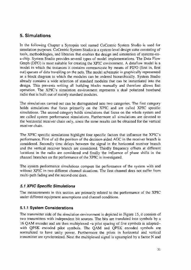
5.1.1 System Considerations

The transmitter side of the simulation environment is depicted in Figure 15, it consists oftwo transmitters with independent bit sources. The bits are translated into symbols by a16 QAM encoder and are then multiplexed -a pilot spacing of five symbols is adopted­with QPSK encoded pilot symbols. The QAM and QPSK encoded symbols arenormalized to have unity power. Furthermore the pilots in horizontal and verticaltransmitter are synchronized. Next the multiplexed signal is upsampled by a factor Nand

31

modified by a root-raised cosine pulse shaping filter before leaving the transmitter. Theroot-raised cosine filter has a rolloff factor of 0.34 and a cutoff frequency that isnormalized to the sample frequency of O.S/N. Additionally the transmitter feeds the barepilot sequences as a reference to the receiver. Consequently there will be no need for pilotdetection in the receiver.

Data In (Bits) . "011010

Pilots In (Bits) .. ·001101

Data In (Bits) ···110100

Pilots In (Bits) ... 100101

(AIr,

Figure 15: Transmitter structure

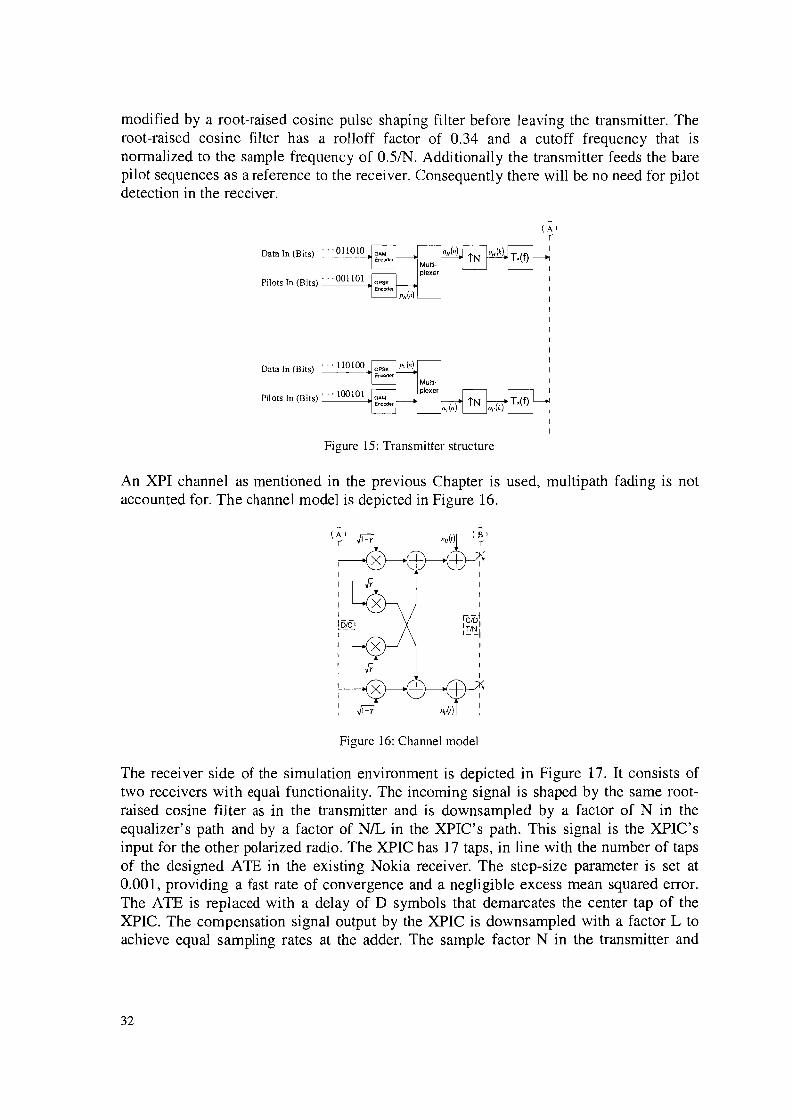
An XPI channel as mentioned in the previous Chapter is used, multipath fading is notaccounted for. The channel model is depicted in Figure 16.

(A I

r

,,,1,

IciDj

'TIN'1--1II

I

I

Figure 16: Channel model

The receiver side of the simulation environment is depicted in Figure 17. It consists oftwo receivers with equal functionality. The incoming signal is shaped by the same root­raised cosine filter as in the transmitter and is downsampled by a factor of N in theequalizer's path and by a factor of NIL in the XPIC's path. This signal is the XPIC'sinput for the other polarized radio. The XPIC has 17 taps, in line with the number of tapsof the designed ATE in the existing Nokia receiver. The step-size parameter is set at0.001, providing a fast rate of convergence and a negligible excess mean squared error.The ATE is replaced with a delay of D symbols that demarcates the center tap of theXPIC. The compensation signal output by the XPIC is downsampled with a factor L toachieve equal sampling rates at the adder. The sample factor N in the transmitter and

32

receiver is set to 4 to be able to insert fractional delays of 14 symbol into the model. In theexisting Nokia radio this upsampling is done to simplify the analog filter conditions.

Data au t (Bits)... 100101

1---- Data Out (Bits)

f-------o{+ ",(n)

-(B1

r

i

Figure 17: Receiver structure

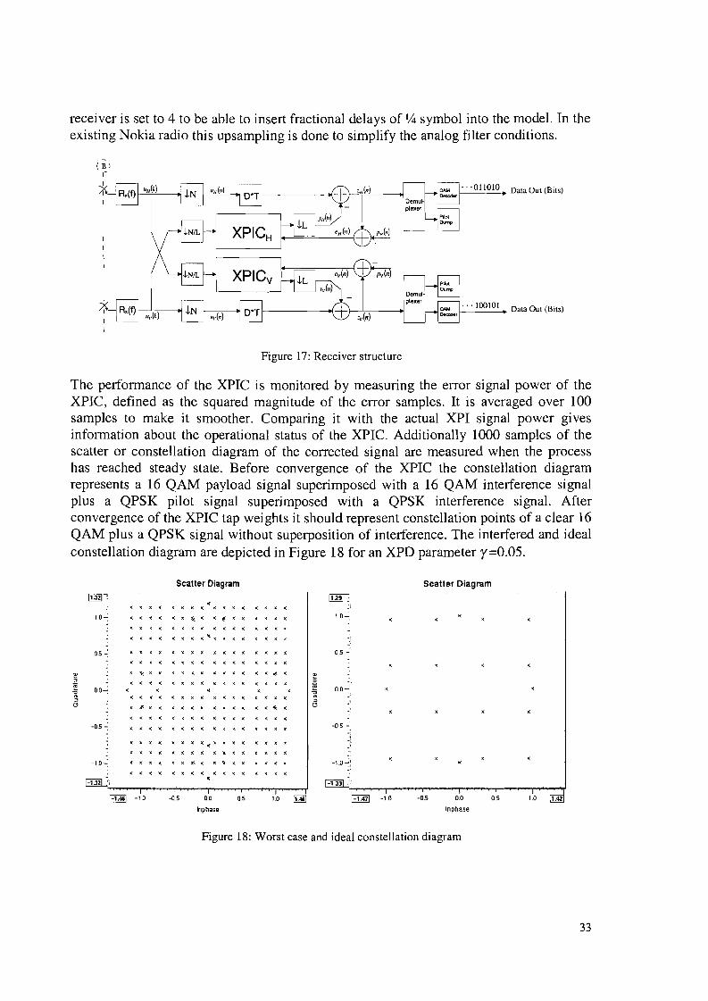
The performance of the XPIC is monitored by measuring the error signal power of theXPIC, defined as the squared magnitude of the error samples. It is averaged over 100samples to make it smoother. Comparing it with the actual XPI signal power givesinformation about the operational status of the XPIC. Additionally 1000 samples of thescatter or constellation diagram of the corrected signal are measured when the processhas reached steady state. Before convergence of the XPIC the constellation diagramrepresents a 16 QAM payload signal superimposed with a 16 QAM interference signalplus a QPSK pilot signal superimposed with a QPSK interference signal. Afterconvergence of the XPIC tap weights it should represent constellation points of a clear 16QAM plus a QPSK signal without superposition of interference. The interfered and idealconstellation diagram are depicted in Figure 18 for an XPD parameter r=0.05.

Scatter Diagram

0.5 ~

1.0 1.420.50.0

Inphas.

-0.5-1.47 -1.0

-0.5 ~.

-\.0-:'.,

10"':

Scatter Diagram

< < < < < <<

< < < < < , <<< < < < < < " < < ~ < < < < < <

< < < < < <, < < < < < < < . < < , < < .

< < < < < < < < < < < < < < . <, < < < < < < < < < < < < < < <,

'", , < , < , < < < ,

'",

< < < < < < < < < < < < < < , << < < <

< < < < , < , < , < , < < < , <, '" , < , < < < , '" << < < < < < < < < < < < < < < ,< < < • < < < < < < < < < < • ,< , , < < < < < < '

, < < < < < ,< < < , < < < < < x < < < . < <, < < < , l; < < '" < ,< < < < < < < < < , < < < < < <

<

-1.46 -lD -0.5 0.0 0.5 10 1.46

Inphas.

10"':

0.0"':

05 ~.

-0.5 ~

-10-':

Figure 18: Worst case and ideal constellation diagram

33

5.1.2 Positioning the Decision Aided AGe

5.1.2.1 Problem Sketch

Parts of the receiver and especially the ATE and the XPIC are decision aided blocks. Thismeans that their operation depends upon the regenerated pilots. This poses high demandson the pilot detection. Loss of pilot synchronization is not tolerated. Varying delays in thereceiver are therefore not allowed. Hence it is highly preferable to have an equalizer filterstructure with a fixed center tap. Fixing the center tap means setting one tap weight to afixed value, nonnally one. The result is that this kind of equalizer is not able tocompensate the small remaining attenuation or amplification effects after the NDA AGe.However an important attribute is that the pilots inside the received data stream shouldhave the same magnitude as the reference pilots. Otherwise a gain error will beintroduced upon calculating the error signal for the XPIC and ATE. Consequently a DAAGC that is able to correct the gain of the received pilots accompanies the ATE. TheAGC compares the magnitude of the received pilots with the magnitude of the referencepilots. After multiplication with a loop constant K the resulting signal is integrated. Thisintegrated signal is subtracted from one, ending up in a gain correction for the receivedsignal. The structure of the AGC is depicted in Figure 19.

X r--~-------

_ m(n)

Figure 19: AGe structure

The relation between in- and output is given by

OUf(n)•

where WAGe (/1) stands for the real AGC coefficient at time 11. In the following simulationsthe real AGC coefficient is set to its optimum value. This optimum value can easily becomputed because the used channel only suffers from a constant attenuation and it doesnot model any fading conditions. The question that arises now is; is there an optimalposition for this AGe?

From a previous study [2] it is known that the XPIC is unable to converge to its optimalcoefficients, due to the fact that the input of the XPIC is contaminated with interferencefrom the other branch. However this study only deals with the operation of the XPIC onitself, based on one simple channel assumption.

34

5.1.2.2 Simulation OutlineFour different receiver structures are considered under a noiseless channel (n(t)=O) andan XPD of FO.05:

1. A receiver structure without AGe.2. A receiver structure with AGC positioned in front of the XPIC, depicted in Figure 20

by <D.3. A receiver structure with AGC positioned parallel to the XPIC, depicted in Figure 20

by@.4. A receiver structure with AGC positioned behind the XPIC. depicted in Figure 20 by

a:>.

In Figure 20 the ATE is represented by the delay D and the AGCs are represented by theparameters W AGC,H and W AGC,v • The delay D is set to D=9 and the downsample factor L isset to L=1.

Data Out (Bits)., ·100101

f---- Data Out (Bits)

ltAGCH

'1/&')Demulplexer

'1/&1)

+-ev(n) +-

",(n)

WAGGV

WAGCH

WAGCV

WAGC1J

"AGCV

AI

I

I

-(B 1

r

~

Figure 20: Different positions for the AGe in the receiver structure

5.1.2.3 Simulation Results

The simulation results of the first situation are depicted in Figure 21. The dotted errorsignal power curve represents the error measured before the XPIC and the solid errorsignal power curve represents the error measured after the XPIC. The error signal powerdecreases to the steady state value of approximately 0.0056. This gain error is caused bythe fact that the reference pilots and the pilots into the data stream do not have the samemagnitude.

35

Scatter Diagram Error Signal Power before and alter XPIC

[[fu] .

0.05-, rV"'V"'V'~M'M"'\""""''';'\''¥''·:'''''''''J.."...v,.I\;\'''<J''!'r''w!tW'''\,'

50004000200a 3QOO

Number of Pilot SymbOls

0.04 -

1,0 1.34a.5

•

aa

Inphase

-0.5-1.34

-os .:.'

Figure 21: Simulation results for situation one

Theoretical analysis results in the same steady state gain error. Calculating the varianceof desired XPIC's response (Eq. (41)) leads to

( 57)

wherea; denotes the variance of the white noise process V H (11). Computing the 17-by-17autocorrelation matrix and the 17-by-1 cross-correlation vector gives

( 58)

( 59)

where I stands for the 17-by-17 identity matrix. The absence of noise results in a;:= 0

and taking into account that QPSK (amplitude 1) encoded pilots are used results ina; := 1. Now substituting Eq. (57), Eq. (58) and Eq. (59) in Eq. ( 18) leads to

( 60)

With the XPD parameter y=0.05 this results in the value 0.0056 for the minimum meansquared error, which is equal to the simulated steady state value of the error signal power.

The simulation results for case two are shown in Figure 22. The error signal powerdecreases to the steady state value of approximately 0.0026. In this case both AGCs have

the same gain W AGC,H := W AGC,V = 1/~. The recei ved pilots and the reference pilots are

at that point equal in size. Afterwards however the output of the XPIC is added to this

36

signal. This output signal YH (11) of the XPIC will contain a small portion of the

transmitted horizontal signal, due to the fact that the input signal U v (11) to the XPIC

contains interference from horizontal path. This interference is now responsible for theintroduced gain error.

004 -'

Error Signal Power before and after XPIC

~.

o.os~ r""~·~\)q."'fJ.)J\':~rl""~~~Wv\J;tJ'\.:,.f"~·rl~·;"''''..,~'''~\~\~l'~'r:/

1000 2000 3000 4000 5000

Number of Pilot Symbols

0.01 ~

~ 003 -'"-

~Vi0 0.02W

1.32

»

•

Scatter Diagram

l.1Hl :

10'-:,

" • lit ..:

0.5 -':

'" •:;~ 0,0--: to."

"::>0 • C'

-0.5 -=

-10--' • .. • ..1-1.341 :

-1.33 -0.5 0.0 0.5

Inphase

Figure 22: Simulation results for case two

Also in this case the steady state gain error obtained via theoretical analysis matches thesimulation. The horizontal and vertical baseband signals are given by

( 61)

Computation of the variance of the desired XPIC's response, the autocorrelation matrixand the cross-colTelation vector result in

2 Y 0 1 2a d= --a~+--al-y n l-y v

( 62)

37

With (JJ=0 and (J; =1 this leads to the following minimum mean squared error

y2J rnin =--

l-y

( 63)

( 64)

( 65)

Substituting the XPD parameter y value in this equation gives a minimum mean squarederror of 0.0026, indeed corresponding to the simulated steady state gain error.

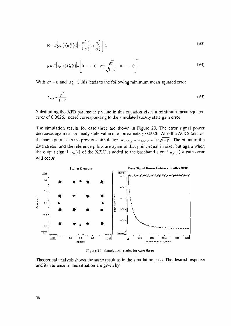
The simulation results for case three are shown in Figure 23. The error signal powerdecreases again to the steady state value of approximately 0.0026. Also the AGCs take on

the same gain as in the previous simulation W AGC,H = W AGC,V = 1/~ . The pilots in the

data stream and the reference pilots are again at that point equal in size, but again whenthe output signal YH (/1) of the XPIC is added to the baseband signal uH (/1) a gain errorwill occur.

Scatter Diagram

l!SI ~

1.0~

", It ..,

05 ~

'"~

"16 0.0-':· •~:>0 • .' •

-05 -'

-1.0-': *' .. .. .,1-1.341 :

-1.33 -0.5 0.0 0.5

Inphase

•It

•1.32

Error Signal Power before and after XPIC

~.

0.05 ~ '1''~,.·~·rtII\)(Jl\.~'\,:tiV~,.,'.J~~~'I~'\':'\''~rl~·l401>..,~\~\.~''~''~!

004 -'

1000 2000 3000 4000 5000

Number or Pilo! Symbols

Figure 23: Simulation results for case three

Theoretical analysis shows the same result as in the simulation case. The desired responseand its variance in this situation are given by

38

1d(n)= r;-::u H(n-D)-aH(Il-D)v 1-y

cr ~= _Y-cr; +_I_ cr ; .l-y l-y

Computation of the autocorrelation matrix and the cross-correlation vector results in

( 66)

( 67)

( 68)

( 69)

Again with cr; =0 and cr; =1 this leads to the following minimum mean squared error

y2J rnin =--

l-y( 70)

Notice that the minimum mean squared error has the same form as in the previoussimulation. When the value of the XPD parameter y is substituted in Eq. ( 70) this willagain lead to a minimum mean squared error of 0.0026. Also in this case the calculatedvalue corresponds to the simulated one.

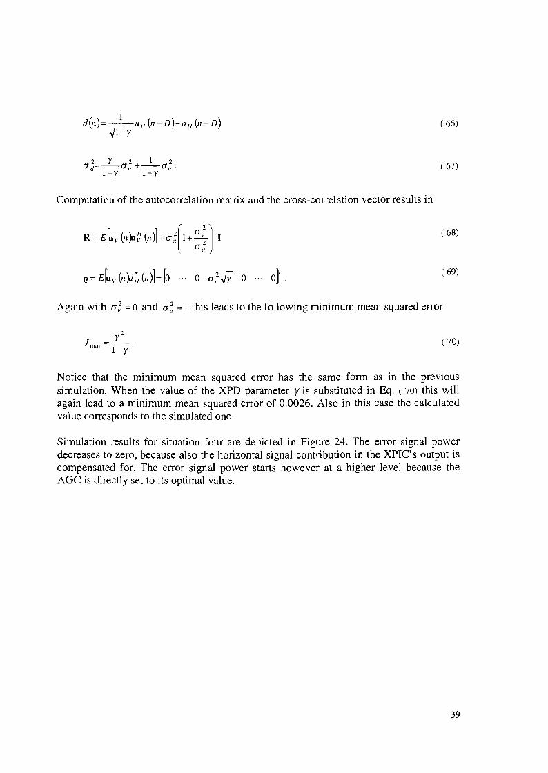
Simulation results for situation four are depicted in Figure 24. The error signal powerdecreases to zero, because also the horizontal signal contribution in the XPIC's output iscompensated for. The error signal power starts however at a higher level because theAGC is directly set to its optimal value.

39

Scatter Diagram Error Signal Power before and after XPIC

lIN' lilliJ :O.O5~ ~\"~h.·\;;.t,.It.y.\v.,\j'\{<'l~'iiI'\;,,,.r\irrr',,t/,,)~·~,,V~·/if,~'Ij~;'I""'~j.W.~1i1tr.,,~~'p:

I D- • • • •004 ....:

0.5 ..:;

• • • • ~"-

OD- • • tu;0

• • • II .n-05 ~

0.01 ~

-1.0- • • • • •0.00.....:

RA2J : 1-0.0031 :

-1.45 -1.0 -05 0.0 05 10 1.4. 1000 2000 3000 4000 5000

Inphase Number 01 Pilol Symbols

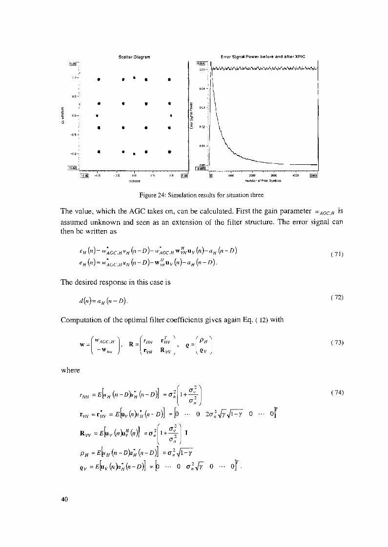
Figure 24: Simulation results for situation three

The value, which the AGC takes on, can be calculated. First the gain parameter WACC.H is

assumed unknown and seen as an extension of the filter structure. The error signal canthen be written as

e H (11)= W:CC,HIIH (11- D)-W:CC,HW~HUV (1I)-aH (11- D)

eH (11)= W:CC,HUH (11- D)-W~tUV (11)-a H (Il- D).

The desired response in this case is

Computation of the optimal filter coefficients gives again Eq. ( 12) with

( 71)

( 72)

W =( ~ACC.H ),l W tot

( 73)

where

'HH "E~H V. ~Dp~ (n~ D)] "";[J<~ JrVH =r~v = E~v(Il~~(n-D)] =[0 ... 0 2a;.JYFY 0 ... orR w "E~vV.~~(n)] "";[J<}PH = E[UH (n - D~~ (n- D)] = a; ~l-Y

Qv =E~vVl}I~(n-D)] =~ ... 0 a;.JY 0 ... of.

40

( 74)

Finally applying this to Eq. ( 14) and taking a?; =a and a; =1 leads to the optimal AGCgain parameter

.J1=Y(1- 2y)W AGC,H = 1-4y(1-y)

( 75)

For this AGC gain parameter the minimum mean squared error Jmill=O and thuscorresponds to the simulation.

5.1.2.4 Interpretation of the Simulation ResultsA receiver structure without AGC will naturally cause a gain error in the error signal.Therefore an AGC should be implemented in the receiver structure. However whenlocated at the wrong position a small gain error will still remain. This gain error is theoutcome of the fact that the AGCs placed in front of the point where the contribution ofthe XPIC is added are not able to account for this contribution. The best position for theAGC from simulation point of view as well as from theoretical point of view is pointedout to be behind the XPIC.

However, equally good results can be achieved when the error signal for the AGC isderived behind the XPIC, but when the gain correction takes place in front of the XPIC orparallel to the XPIC. Though this will lead to a smaller loop bandwidth of the AGC,decreasing the tracking capability. However this decrease is small only depending on thecenter tap position of the ATE. Considering this it might be a good idea to place the gaincorrection in front of the XPIC and ATE, keeping the gain of their input signals at aconstant level.

5.1.3 Timing Sensitivity of the XPIC

5.1 .3.1 Problem SketchThe horizontal and vertical receiver links belong to two separate radios. This means thatthe input signals of the XPICs have to be fed from one radio to the other by means of acable connection. Such a cable connection will cause an unknown signal delay.Furthermore the two radio paths may differ, which can result in an additional delay.Consequently the received signal and the input of the XPIC are not synchronized. Thedelay most likely consists of a number of symbol delays plus a fractional delay. Thequestion now is; do these delays have any influence on the XPIC's performance?

Previous work [10] showed that baud spaced XPICs and ATEs need exactsynchronization of the time phase between horizontal and vertical path in order to

achieve the best cancellation performance. This synchronization is done by means of anElastic Storage (ES) in front of the XPIC's input. When fractionally spaced XPICs areused there will be no need for clock synchronization [11].

41

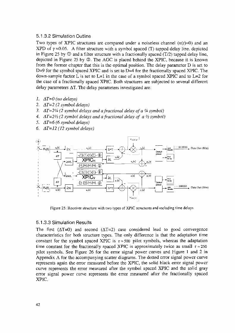
5.1.3.2 Simulation OutlineTwo types of XPIC structures are compared under a noiseless channel (n(t)=O) and anXPD of y =0.05. A filter structure with a symbol spaced (T) tapped delay line, depictedin Figure 25 by CD and a filter structure with a fractionally spaced (T/2) tapped delay line,depicted in Figure 25 by ell. The AGC is placed behind the XPIC, because it is knownfrom the fonner chapter that this is the optimal position. The delay parameter D is set toD=9 for the symbol spaced XPIC and is set to D=4 for the fractionally spaced XPIC. Thedown-sample factor L is set to L=l in the case of a symbol spaced XPIC and to L=2 forthe case of a fractionally spaced XPIC. Both structures are subjected to several differentdelay parameters ~T. The delay parameters investigated are:

1. ,1T=O (no delays)2. ,1T=2 (2 symbol delays)3. ,1T=21/4 (2 symbol delays and a fractional delay ofa lI4 symbol)4. ,1T=2Vz (2 symbol delays and a fractional delay of a Vz symbol)5. ,1T=6 (6 symbol delays)6. ,1T=12 (12 symbol delays)

-(B 1

rX

I

II

II

I

I

I

I

I

I

I

AIII

HAGC /{

I

ulI (,,)

-E:J-.E:I-El--0 CDXPICH

~@

-E:J-.E:I-El--0 CD+-p,(n)

XPICv e,-(n)

~~

",_in)

~1:WCV

~

Figure 25: Receiver structure with two types of XPIC structures and including time delays

5.1.3.3 Simulation Results

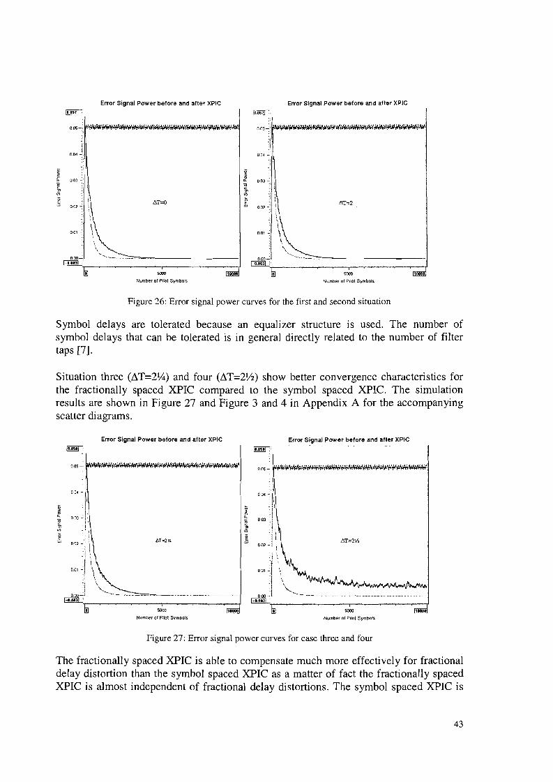
The first (i1T=O) and second (i1T=2) case considered lead to good convergencecharacteristics for both structure types. The only difference is that the adaptation timeconstant for the symbol spaced XPIC is r =:: 500 pilot symbols, whereas the adaptationtime constant for the fractionally spaced XPIC is approximately twice as small r =:: 250

pilot symbols. See Figure 26 for the error signal power curves and Figure 1 and 2 inAppendix A for the accompanying scatter diagrams. The dotted error signal power curverepresents again the error measured before the XPIC, the solid black error signal powercurve represents the error measured after the symbol spaced XPIC and the solid grayerror signal power curve represents the error measured after the fractionally spacedXPIC.

42

Error Signal Power before and after XPIC Error Signal Power before and aller XPIC

0.04 0.04

~a.. 003

~in

~a.. 0.03 .:.

~.;;

10000

L'>.T=2

5000

Number of Piiol Symbols

10000

6.T=O

SOOO

Number of Pilot Symbols

0.00-':'

1".'31 :,--~-~~-~....,..-~~-~-...,.--,J

~ 0.02

Figure 26: Error signal power curves for the first and second situation

Symbol delays are tolerated because an equalizer structure is used. The number ofsymbol delays that can be tolerated is in general directly related to the number of filtertaps [7].

Situation three (~T=21;4) and four (~T=2Y2) show better convergence characteristics forthe fractionally spaced XPIC compared to the symbol spaced XPIC. The simulationresults are shown in Figure 27 and Figure 3 and 4 in Appendix A for the accompanyingscatter diagrams.

Error Signal Power before and aller XPIC Error Signal Power before and aller XPIC

005- ~"~~WVfJ<l/lwv.\~w~~

I

." _==-_ _.- - .

0.0< C rJ,

:i'j

0.Dl ci

0.00-:;

1·....31'r -~~-~--..,......--~----...--r5000

Number of Pilot Symbol&

10000 500D

Number of Pilot Symbols

,....

Figure 27: Error signal power curves for case three and four

The fractionally spaced XPIC is able to compensate much more effectively for fractionaldelay distortion than the symbol spaced XPIC as a matter of fact the fractionally spacedXPIC is almost independent of fractional delay distortions. The symbol spaced XPIC is

43

still able to compensate for a fractional delay of 14 with almost no performance loss. Onlyfor the case of a fractional delay of 1;2 the performance is visibly degraded. The errorsignal power level decreases, but an error remains.

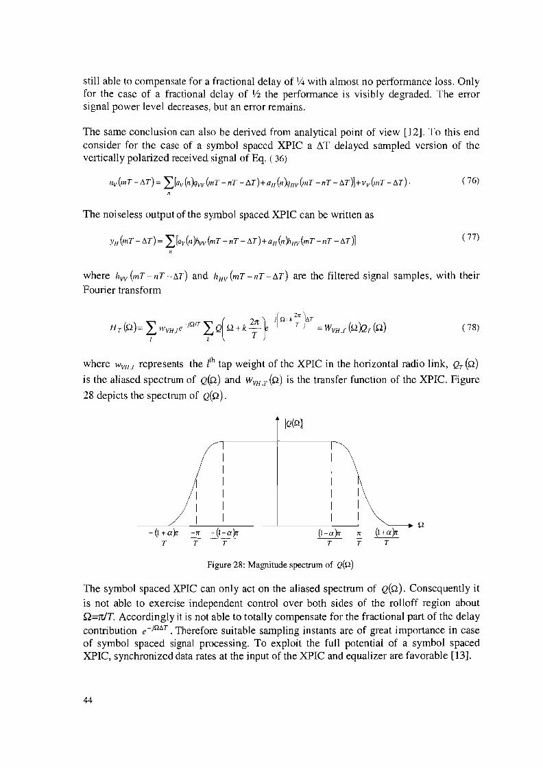
The same conclusion can also be derived from analytical point of view [12]. To this endconsider for the case of a symbol spaced XPIC a ~T delayed sampled version of thevertically polarized received signal of Eq. (36)

( 76)

The noiseless output of the symbol spaced XPIC can be written as

( 77)

where hw(mT-nT-I:lT) and hHV(mT-nT-t:..T) are the filtered signal samples, with theirFourier transform

( 78)

where WVH,l represents the zth tap weight of the XPIC in the horizontal radio link, QT(n)is the aliased spectrum of Q(n) and WVH ,T (n) is the transfer function of the XPIC. Figure

28 depicts the spectrum of Q(n).

I II II II II II I

_-----,-------L':--_'-----------;_-----,--__-----' ~_ __;__"_:_- Q

- (1 +a)ir -rr -(I-a)n- (I-a)n- rr (I+a)n-T T T T T T

Figure 28: Magnitude spectrum of Q(Q)

The symbol spaced XPIC can only act on the aliased spectrum of Q(n). Consequently itis not able to exercise independent control over both sides of the rolloff region aboutQ=mT. Accordingly it is not able to totally compensate for the fractional part of the delaycontribution e-jQ/:;T. Therefore suitable sampling instants are of great importance in caseof symbol spaced signal processing. To exploit the full potential of a symbol spacedXPIC, synchronized data rates at the input of the XPIC and equalizer are favorable [13].

44

On the other hand for the case of a fractionally spaced XPIC with spacings of T' thefiltered signal spectrum is given by

( 79)

When T'<T/(l+a) QT'(n) is not aliased. Therefore the fractionally spaced XPIC is able to

compensate for the delay contribution e-jQl!.T, because of the fact that only the k=O termis of concern. Then after the filter operation the output is re-sampled at symbol rate.

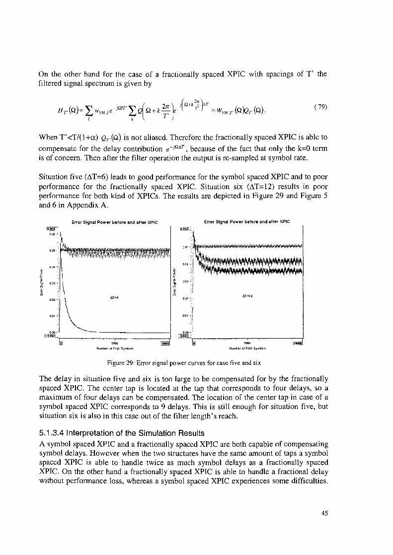
Situation five (~.T=6) leads to good performance for the symbol spaced XPIC and to poorperformance for the fractionally spaced XPIC. Situation six (~T=12) results in poorperformance for both kind of XPICs. The results are depicted in Figure 29 and Figure 5and 6 in Appendix A.

0.00"':1

ITOW :.-r-~--~-"""",-~---""--r

~0-

~ 0.03-on

Error Signal Power before and after XPIC

500J

Number or PUol Symbols

10000

Error Signal Power before and after XPIC

5000

Number of Pilot Symbols

t ....

Figure 29: Error signal power curves for case five and six

The delay in situation five and six is too large to be compensated for by the fractionallyspaced XPIC. The center tap is located at the tap that corresponds to four delays, so amaximum of four delays can be compensated. The location of the center tap in case of asymbol spaced XPIC corresponds to 9 delays. This is still enough for situation five, butsituation six is also in this case out of the filter length's reach.

5.1.3.4 Interpretation of the Simulation ResultsA symbol spaced XPIC and a fractionally spaced XPIC are both capable of compensatingsymbol delays. However when the two structures have the same amount of taps a symbolspaced XPIC is able to handle twice as much symbol delays as a fractionally spacedXPIC. On the other hand a fractionally spaced XPIC is able to handle a fractional delaywithout performance loss, whereas a symbol spaced XPIC experiences some difficulties.

45

Though when a symbol spaced XPIC is combined with a Elastic Storage (ES) it willperform equally well, due to the capability of an ES to synchronize data streams [14]. Ofcourse for this purpose an extra module has to be inserted resulting in a more complexschematic. Concluding it can be said that the results are similar to those in the literature.

Finally a remark should be made: It is known that fractionally spaced adaptive filterstructures can lead to long term instability, while it is not able to adapt to frequenciesoutside the rolloff region, due to the fact that the input spectrum is zero for thosefrequencies. Deeper investigation of the fractionally spaced XPIC should clarify this.Several possible algorithms are presented in the literature to overcome this problem. Thesimple tap-leakage algorithm [15] and the more complicated algorithm presented byUyematsu and Sakaniwa [16] are two examples.

5.1.4 Frequency Offsets between the Oscillators of the Radio

5.1.4.1 Problem SketchThe dual polarized radio link consists of two transmitters and two receivers. Eachtransmitter consists of a modulator that converts the signal from baseband to IF and anup-converter that raises the frequency to RF. Each receiver consists of a down-converterthat lowers the frequency to IF and a demodulator that converts the IF signal into abaseband signal. Every conversion operation at transmitter or receiver involves a localoscillator. Yet it is impossible to design local oscillators that have identical frequencybehavior. For this reason frequency offsets occur between the signals in the horizontaland the vertical radio link at transmitter as well as receiver side. These frequency offsetscan be eliminated when the local oscillators of the up- and down-converters and the localoscillators of the modulator and demodulator are synchronized. The question that arises;do these frequency offsets degrade the performance of the XPIC?

Previous studies [9], [11], [14] state that a critical issue is system synchronization,suggesting synchronization of the local oscillators at the receiver side. Withsynchronization of the RF/IF down-converters and IF/BB demodulators the interferingand compensating signal have the same zero-frequency offset. This means that the XPICdoes not have to compensate any frequency difference. An advantage of this concept isthe independence of the XPIC operation from the lock in state of the carrier recoveryloop [9]. The signal exchange takes place at IF, which means that extra demodulators,AID converters, ND AGCs, etc. are needed. Apart form the signal exchange connectionthe horizontally and vertically polarized receiver only need one more interconnection, tosynchronize the local oscillators of the down-converters.

Other studies [8], [10], [17], [18] suggest synchronization of the modulators and up­converters. This ensures identical center frequencies of both transmitted spectra. Zero­frequency offset between the received horizontally and vertically polarized signal is metby the individual carrier recovery loops in the receiver [8], [18]. The exchange of datacan then be done after AID conversion at baseband, which will save extra AID convertersand demodulators for the XPIC branches.

46

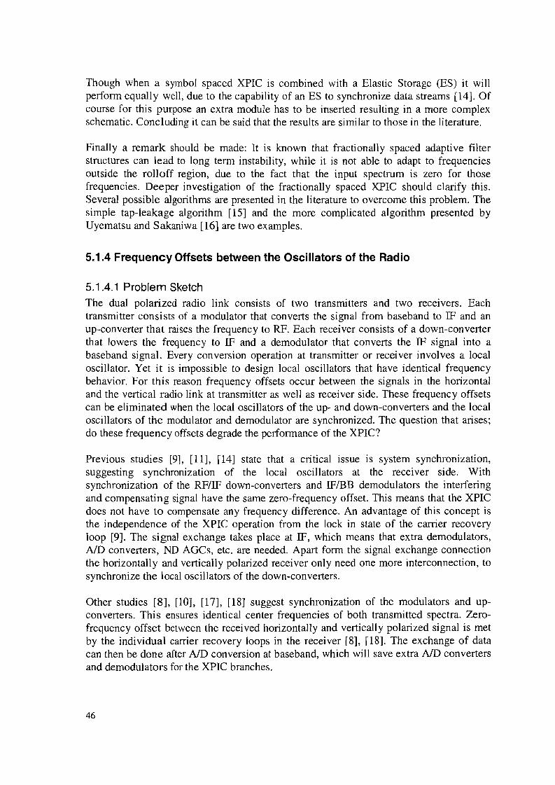
5.1 .4.2 Simulation OutlineFour different situations concerning frequency offsets are considered for a noiselesschannel (n(t)=O) and an XPD of y=O.05. The receiver is implemented with a fractionallyspaced XPIC resulting in a delay of D=4 and a downsample factor of L=2.

1. A situation with no frequency offsets in the dual polarized radio is evaluated, which isachieved by sharing or synchronizing the oscillators in the horizontally and verticallypolarized radio links. A big disadvantage is the mutual connections between the Hand V transmitters and receivers.

2. A situation with a frequency offset of 200 kHz at transmitter side is considered. Sucha frequency offset is typical for radios that operate in the 18 GHz range according tothe ETSI specifications [19]. Thus only the oscillators at the receiver side are sharedor synchronized. The frequency offset is indicated by 11fT and is included in thevertical path, depicted in Figure 30 by 0.

3. A situation with a frequency offset of 20 kHz at receiver side is considered. This is atypical value because of the fact that the decision aided modules are becoming activewith a residual zero-frequency offset of 20 kHz. Now only the oscillators at thetransmitter side are shared or synchronized, resulting in identical carrierfrequencies. The frequency offset is indicated by I1fR and is included in the verticalpath, depicted in Figure 30 by @.

4. A situation with a frequency offset of 200 kHz between the transmitters and afrequency offset of 20kHz between the receivers is observed. The frequency offset atthe transmitter side is indicated by 11fT and the frequency offset at the receiver side is

indicated by I1fR' both are included in the vertical path, depicted in Figure 30 by (1).

(A l

rI

I

I

II

I

I

LD.!.~I

I

c=-----, II

I

I

Figure 30: Frequency offsets at transmitter and receiver sides

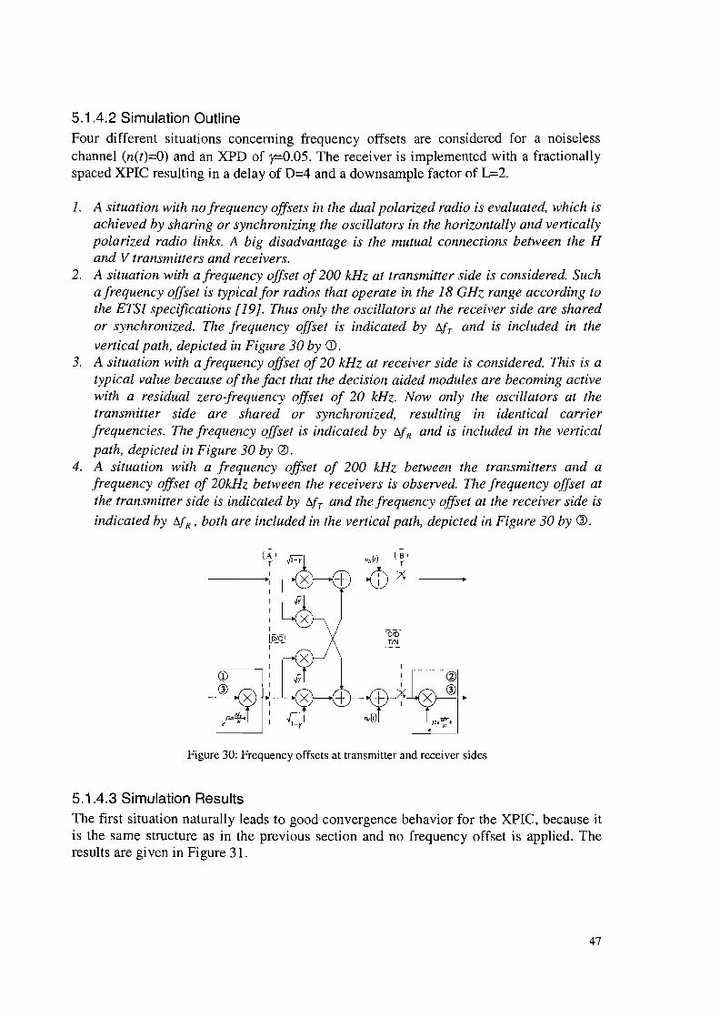
5.1.4.3 Simulation ResultsThe first situation naturally leads to good convergence behavior for the XPIC, because itis the same structure as in the previous section and no frequency offset is applied. Theresults are given in Figure 31.

47

5000

Number of Pilot Symbols

Error Signal Power before and alter XPIC

10,0551 :

0'05~. r.rl).\"'i~b'\io-..lWt~.>I"\l-~Jl\I.,'\lIW\il\lo\O,,"iW\4\Io~~

II0,04 ~: I

J0,03 ..:. I

: I\

002 ~J !

'" -' \\ ...

...~~._.__._~_ ••••~ • __m • __._._••" _

10 1.290500

Inphase

Scatter Diagram

-0.5-1.29

10-:

0.5 ~

0.0"':'

-05 ....:

-1.0-":'

Figure 31: Simulation results for situation one

The results for situation two are depicted in Figure 32. In this case there exists afrequency offset between horizontally and vertically polarized signal in the transmitter.This frequency offset is not visible between the XPIC's error signal and the XPIC's inputsignal, since they originate from the same polarized radio. A frequency offset only existsbetween the horizontally polarized signal parts and the vertically polarized signal parts.However all signals will suffer a frequency offset compared to the zero frequency whenthe demodulator is not able to convert the IF signal to a zero-frequency baseband signal.But this frequency offset is the same for all the signals because the demodulators areshared or synchronized. In time domain a frequency offset is a rotation of the phase.When interference and XPIC input signal have the same rotation velocity this will nothave an effect on the performance.

Scatter Diagram Error Signal Power before and alter XPIC

1.0": 0.05-:

::1:j

O~ -I:

-1.0-:

-1.58 -1.0 -0.5 00

Inphase

05 10 1.58 5000

Number of Pilot SymbOls

10000

Figure 32: Simulation results for situation two

48

This situation enforces no restrictions on the oscillators at the transmitter side and signalexchange is made at IF level, thus only an interconnection between the down-convertersin the receiver should be made [11], [13], [14].

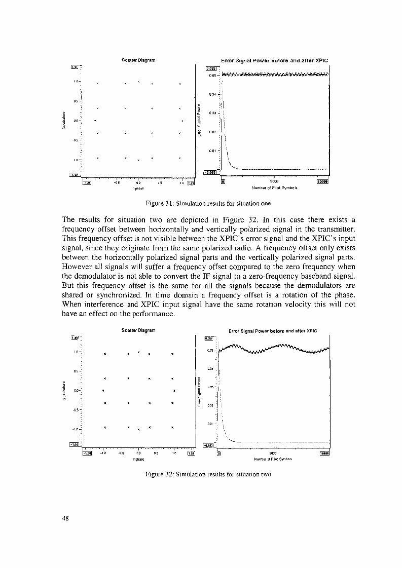
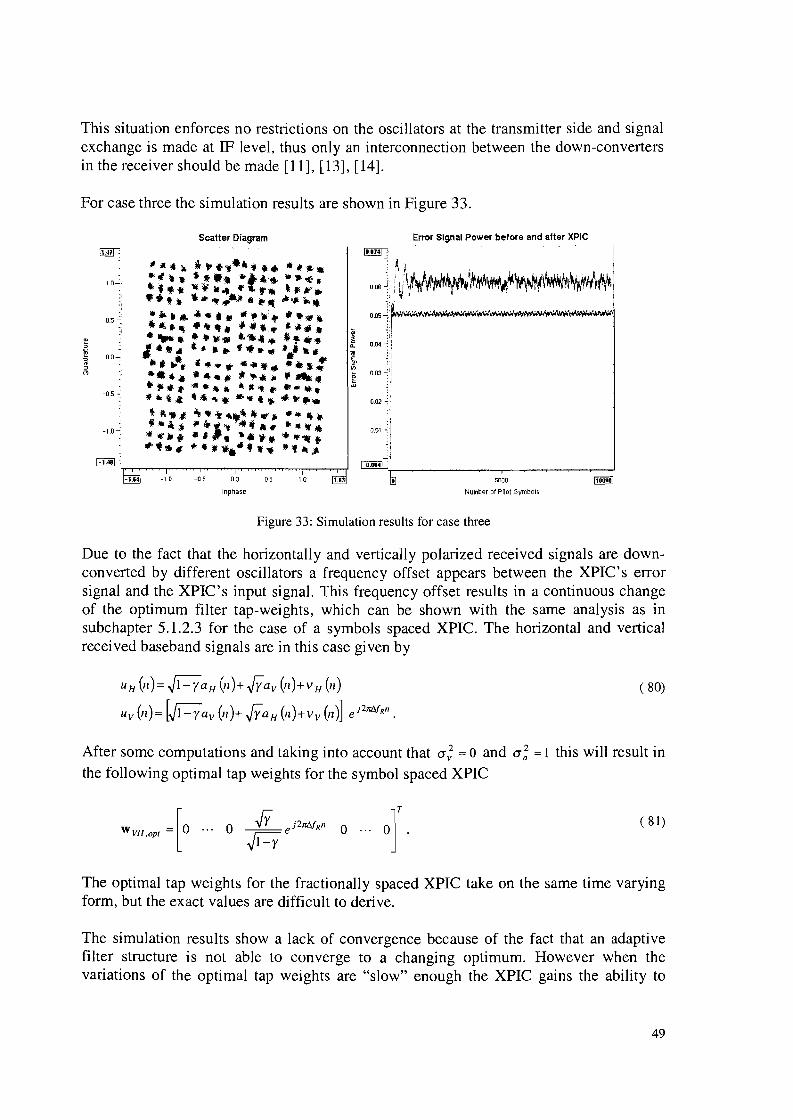
For case three the simulation results are shown in Figure 33.

Scatter Diagram Error Signal Power before and alter XPIC

001 ~i-,-,~ I

--,i1-•.••0' :....-~~_....-~_,----_~ __--,-......--,'

-1.&4 -10 -0.5 0.0 0.5

Inphase

10 1.63 SOOO

Number of Pilot Symbols'.000

Figure 33: Simulation results for case three

Due to the fact that the horizontally and vertically polarized received signals are down­converted by different oscillators a frequency offset appears between the XPIC's errorsignal and the XPIC's input signal. This frequency offset results in a continuous changeof the optimum filter tap-weights, which can be shown with the same analysis as insubchapter 5.1.2.3 for the case of a symbols spaced XPIC. The horizontal and verticalreceived baseband signals are in this case given by

UH 01)= ~1-yaH (11)+ .jYav 01)+vH(II)

Uv (11)= [~I-yav (1I)+.jYaH (II)+V V (II)] ej21r1J.f R

Il •

( 80)

After some computations and taking into account that a; = 0 and a; = 1 this will result inthe following optimal tap weights for the symbol spaced XPIC

( 81)

The optimal tap weights for the fractionally spaced XPIC take on the same time varyingform, but the exact values are difficult to derive.

The simulation results show a lack of convergence because of the fact that an adaptivefilter structure is not able to converge to a changing optimum. However when thevariations of the optimal tap weights are "slow" enough the XPIC gains the ability to

49

track those variations to some extent. To what degree depends on the value for the step­size parameter ~. An algorithm with a larger step-size parameter is able to track fastervariations than a algorithm with smaller step-size parameter, but as a consequence abigger excess mean squared error of the tap weights (see Eq. ( 28)) in the case of J min * 0

must be permitted. However the step-size parameter cannot be chosen arbitrary. When itis chosen too large the adaptive filter becomes unstable. The range, which the step-sizeparameter is allowed to take on, has been given in Chapter 3. For this case this results in

0< J.l < 0.117 ( 82)

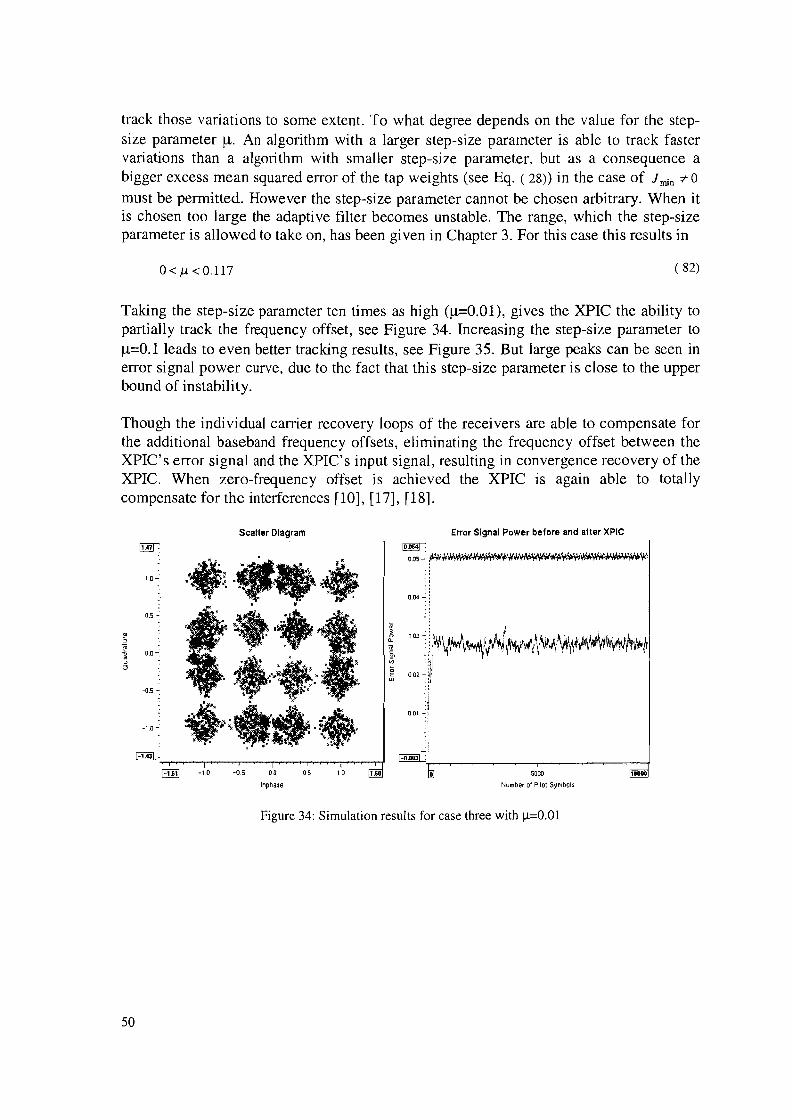
Taking the step-size parameter ten times as high (J..IF0.OI), gives the XPIC the ability topartially track the frequency offset, see Figure 34. Increasing the step-size parameter to~=O.1 leads to even better tracking results, see Figure 35. But large peaks can be seen inerror signal power curve, due to the fact that this step-size parameter is close to the upperbound of instability.

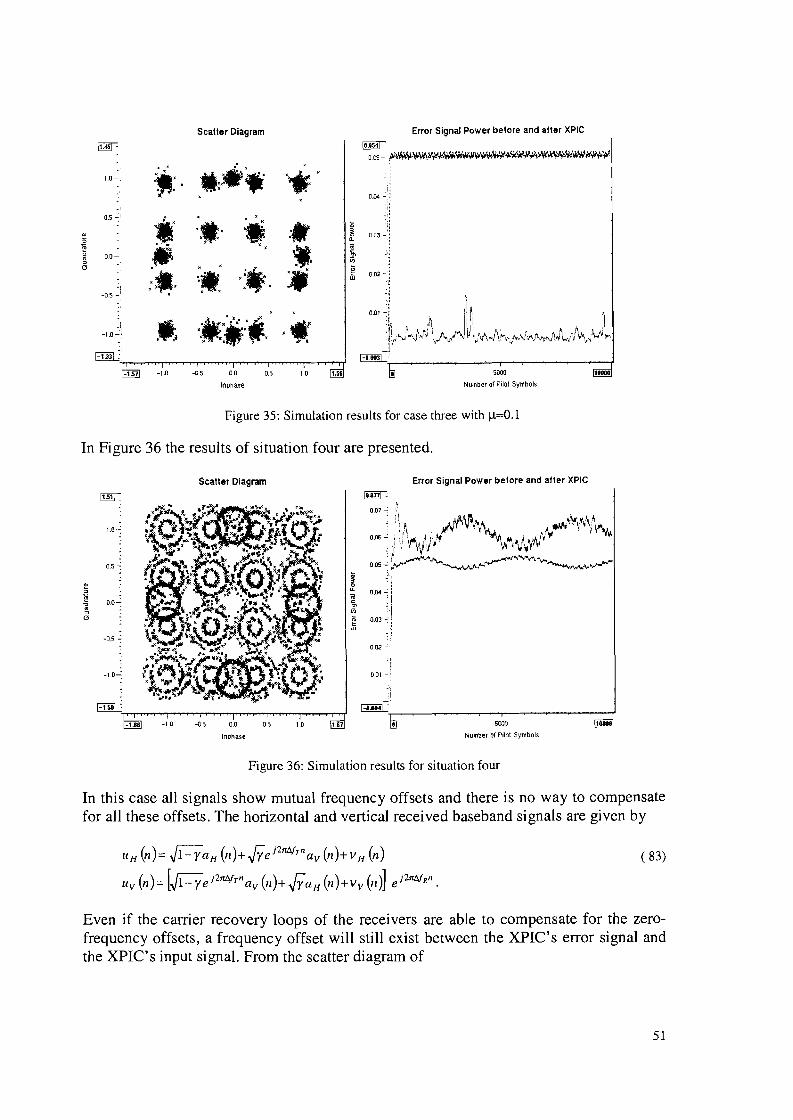
Though the individual carrier recovery loops of the receivers are able to compensate forthe additional baseband frequency offsets, eliminating the frequency offset between theXPIC's error signal and the XPIC's input signal, resulting in convergence recovery of theXPIC. When zero-frequency offset is achieved the XPIC is again able to totallycompensate for the interferences [10], [17], [18].

Scafler Diagram Error Signal Power before and after XPIC

[lliJ .0.05 -. fWWwW~.fIv/.j,W.·1>W~Vtv.WVlV/'iI';'W.WVMWV/~V.V."'W

0.04 ..:. :

~ .: . I .'i 0 03 ~i,~\)i~IIttt~~~'~JJ~J\~vrt.lr\V'~J1AJf\\(~!/#f1WrrJi\rl#fl~Vi ~g 002 ~~Iw .:,

:J001 ~:

-1.61 -1.0 -{)s 00 0.5

Inphas.

10 1.60 5000

Number of Pilot Symbols

1.080

Figure 34: Simulation results for case three with ~=0.01

50

Scatter Diagram Error Signal Power before and after XPIC

._,, ,,

0.04 ..:.~~

:~1,~ ,

0.03 -:

0.02 ~i.'-~ ,.

0.01 -i ":1\ il'l [i, [\·r'llo:,,,,,I, \' , .~.~r"!. I',", \01\. [J<jY \ i ... _~ '\r If r~ ;11,)." •.,1 l~""I\.~J1f'.,r;. "'''t>.Ji",} \ ,hflr~ ~[\,.(~.,....~1 '.[' \i v'" V" " \1 '> , '" ~ ~{n"" "'''. '" '1"- ....~. ',rr

1-0.0031 .~.-_~- ---r--"-- - __--,l

,:' ,1i:*_'I'••:_, ~-,

0.0-

1.0-.

-0.5 -'

-151 -1.0 -05 0.0 0.5

Inphase

1.0 1.56 5000

Number of Pilot Symbols

ooסס1

Figure 35: Simulation results for case three with J.l=O.l

In Figure 36 the results of situation four are presented.

Scalier Diagram Error Signal Power before and after XPIC

0.01 -;

-1.66 -1.0 -05 0.0 05

Inphase

1.0 1.61 5000

Number of Pilot Symbols

100ee

Figure 36: Simulation results for situation four

In this case all signals show mutual frequency offsets and there is no way to compensatefor all these offsets. The horizontal and vertical received baseband signals are given by

UH (11):= J1-yaH (11)+f(ej21r4frnav (n)+v H(n)

Uv (n):= [J1-yeJ2m~hnav (n)+f(aH (n)+vv (11)] e j21r1'.fRn.

( 83)

Even if the carrier recovery loops of the receivers are able to compensate for the zero­frequency offsets, a frequency offset will still exist between the XPIC's error signal andthe XPIC's input signal. From the scatter diagram of

51

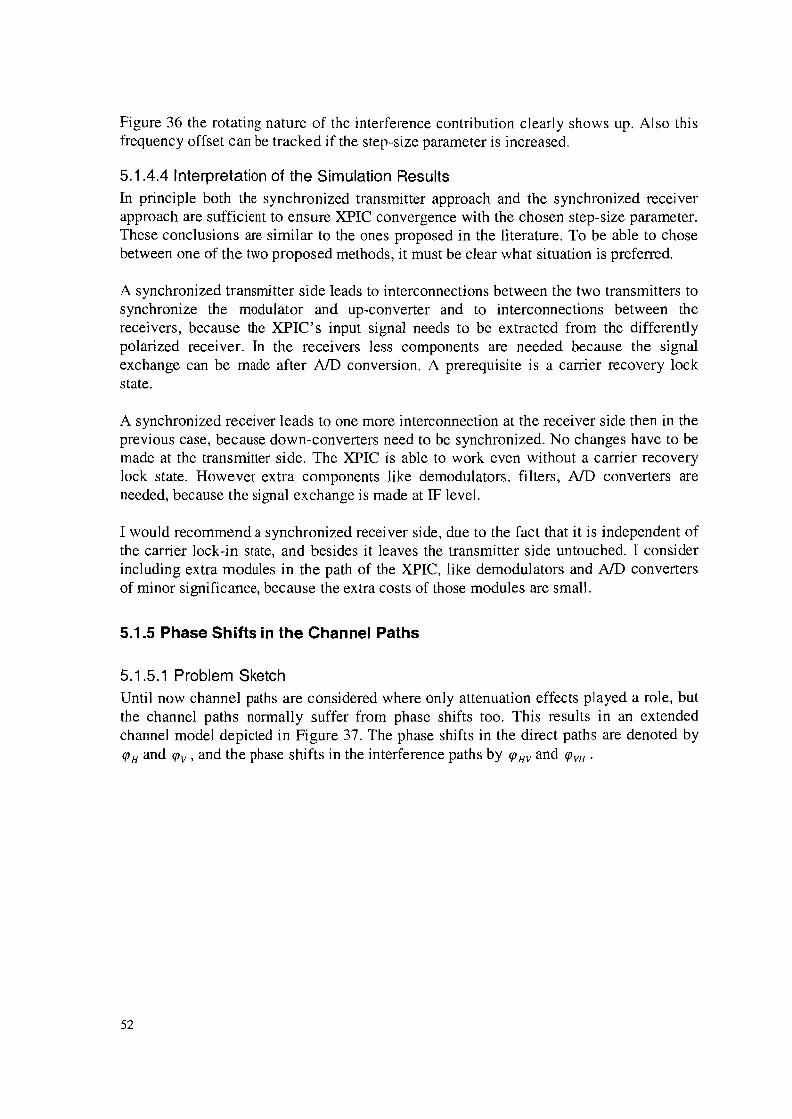
Figure 36 the rotating nature of the interference contribution clearly shows up. Also thisfrequency offset can be tracked if the step-size parameter is increased.

5.1.4.4 Interpretation of the Simulation ResultsIn principle both the synchronized transmitter approach and the synchronized receiverapproach are sufficient to ensure XPIC convergence with the chosen step-size parameter.These conclusions are similar to the ones proposed in the literature. To be able to chosebetween one of the two proposed methods, it must be clear what situation is preferred.

A synchronized transmitter side leads to interconnections between the two transmitters tosynchronize the modulator and up-converter and to interconnections between thereceivers, because the XPIC's input signal needs to be extracted from the differentlypolarized receiver. In the receivers less components are needed because the signalexchange can be made after AID conversion. A prerequisite is a carrier recovery lockstate.

A synchronized receiver leads to one more interconnection at the receiver side then in theprevious case, because down-converters need to be synchronized. No changes have to bemade at the transmitter side. The XPIC is able to work even without a carrier recoverylock state. However extra components like demodulators, filters, AID converters areneeded, because the signal exchange is made at IF level.

I would recommend a synchronized receiver side, due to the fact that it is independent ofthe carrier lock-in state, and besides it leaves the transmitter side untouched. I considerincluding extra modules in the path of the XPIC, like demodulators and AID convertersof minor significance, because the extra costs of those modules are small.

5.1.5 Phase Shifts in the Channel Paths

5.1.5.1 Problem SketchUntil now channel paths are considered where only attenuation effects played a role, butthe channel paths normally suffer from phase shifts too. This results in an extendedchannel model depicted in Figure 37. The phase shifts in the direct paths are denoted byqJ Hand qJv , and the phase shifts in the interference paths by qJ HV and qJVH •

52

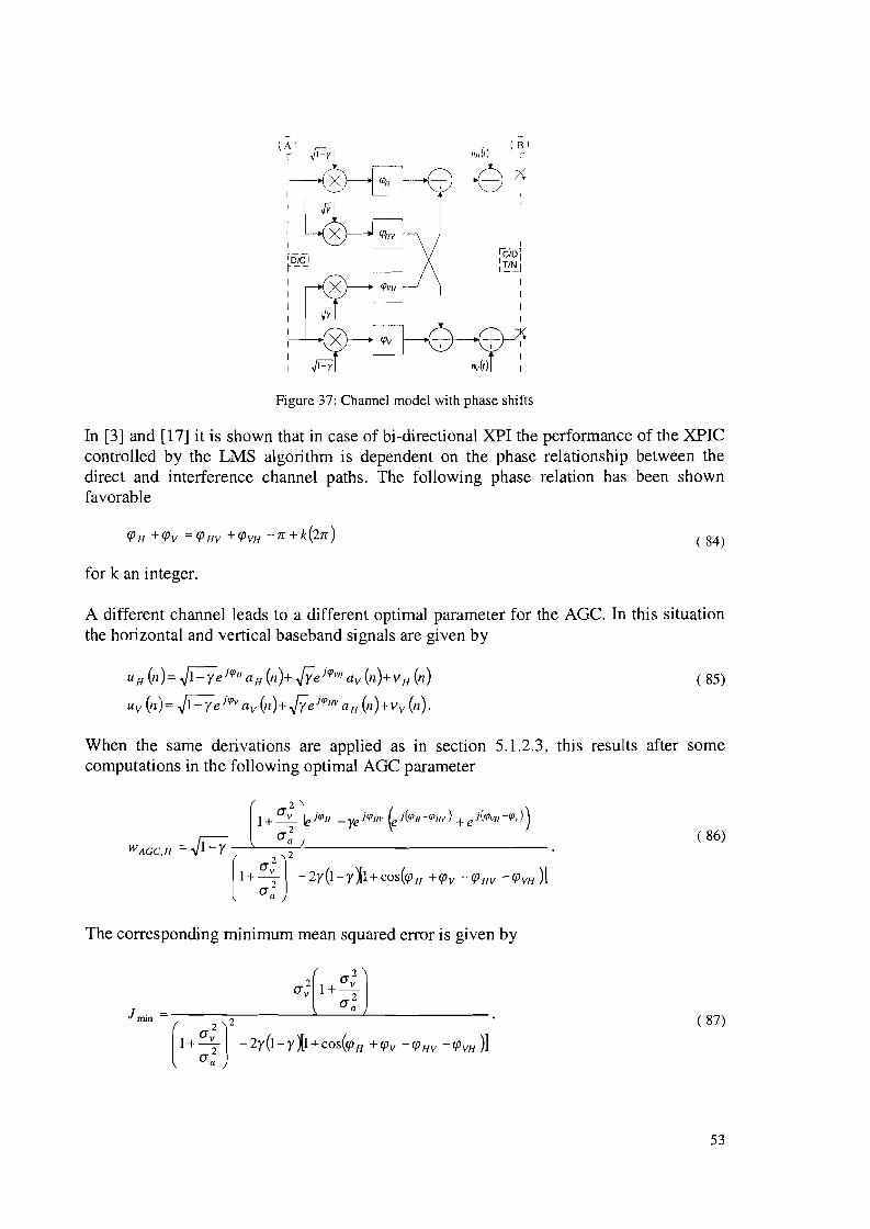
I

I[

II

IreiD]l!!~l

II

II

Figure 37: Channel model with phase shifts

In [3] and [17] it is shown that in case of bi-directional XPI the performance of the XPICcontrolled by the LMS algorithm is dependent on the phase relationship between thedirect and interference channel paths. The following phase relation has been shownfavorable

( 84)

for k an integer.

A different channel leads to a different optimal parameter for the AGe. In this situationthe horizontal and vertical baseband signals are given by

UIi (n)= ~l-y ejl{JII a Ii (11)+ f(e jlfJvlI ay (/1)+ VIi (/1)

Uy (n)= ~ejlfJv a y01)+f(e jlfJllv aH (/1)+V y(/1).

( 85)

When the same derivations are applied as in section 5.1.2.3, this results after somecomputations in the following optimal AGC parameter

1+ a; jlfJlI _yejlfJllv (ej(IfJII-IfJJI\') + ej(IfJVII-IfJ,.))

a 2

W AGe,1i =~ _-"--__~...L--------------

[1+ :~) -2Y(I-rXl+oo,(~" +~, -~'" -~"')]

The corresponding minimum mean squared error is given by

J min = 2

[I +:n -2y(l-y:iJ HO'(~" +~, -~'" -~,,,)]

( 86)

( 87)

53

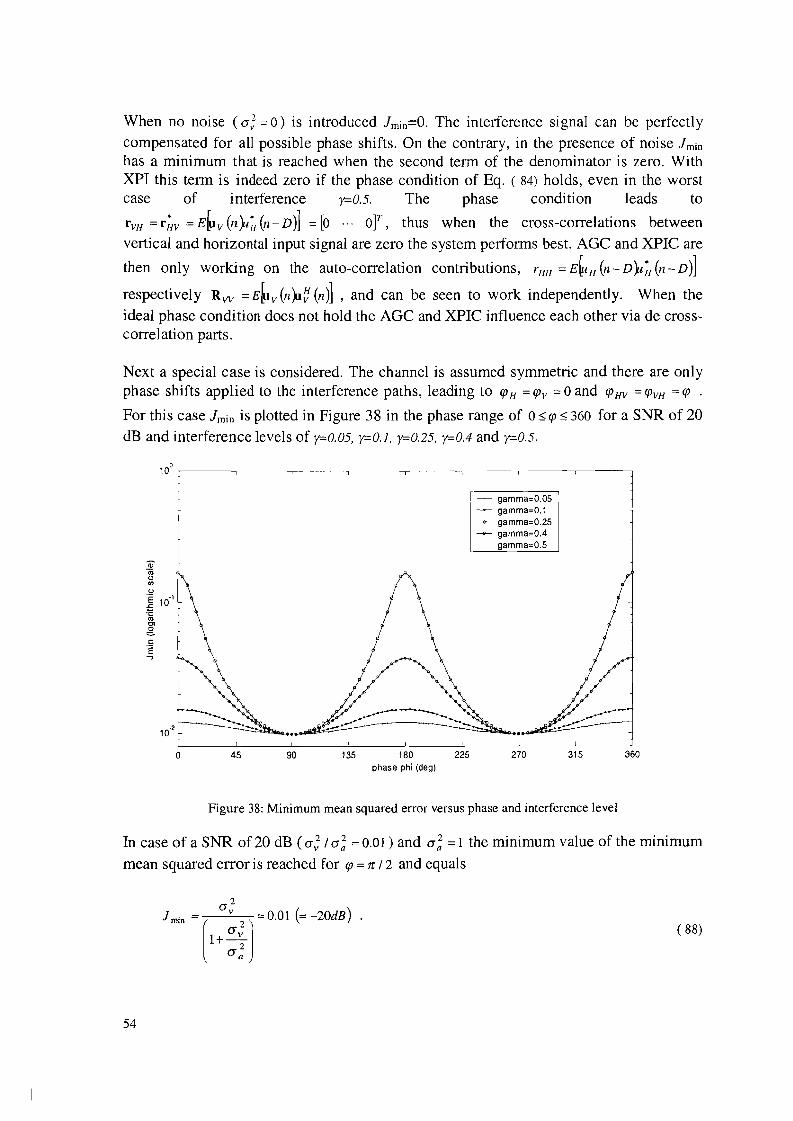
When no noise (0'; =0) is introduced lrnin=O. The inteIference signal can be peIfectlycompensated for all possible phase shifts. On the contrary, in the presence of noise lrnin

has a minimum that is reached when the second term of the denominator is zero. WithXPI this term is indeed zero if the phase condition of Eq. ( 84) holds, even in the worstcase of inteIference y=O.5. The phase condition leads to

rVH =r~v =E~v(ll}t~(n-D)] =[0 ... oy, thus when the cross-correlations betweenvertical and horizontal input signal are zero the system peIforms best. AGC and XPIC are

then only working on the auto-correlation contributions, rHH =E[uH(n-D}t~(n-D)]

respectively R w =E~v(n:Uf(n)] , and can be seen to work independently. When theideal phase condition does not hold the AGC and XPIC influence each other via de cross­correlation parts.

Next a special case is considered. The channel is assumed symmetric and there are onlyphase shifts applied to the inteIference paths, leading to qJ H= qJv = 0 and qJ HV = qJVH = qJ .

For this case lrnin is plotted in Figure 38 in the phase range of 0::5: qJ::5: 360 for a SNR of 20dB and interference levels of y=O.05, y=O.l, y=O.25, y=O.4 and y=O.5.

o10 C-f---~--~---~----~-----.----~----.--

I - gamma~0.05- gamma~0.1

-- gamma=0.25-- gamma=O.4

gamma=0.5

l

o 45 90 135 180 225phase phi (deg)

270 315 360

Figure 38: Minimum mean squared error versus phase and interference level

In case of a SNR of 20 dB ( 0'; /0'; =0.01 ) and 0'; =1 the minimum value of the minimum

mean squared error is reached for qJ = IT / 2 and equals

( 88)

54

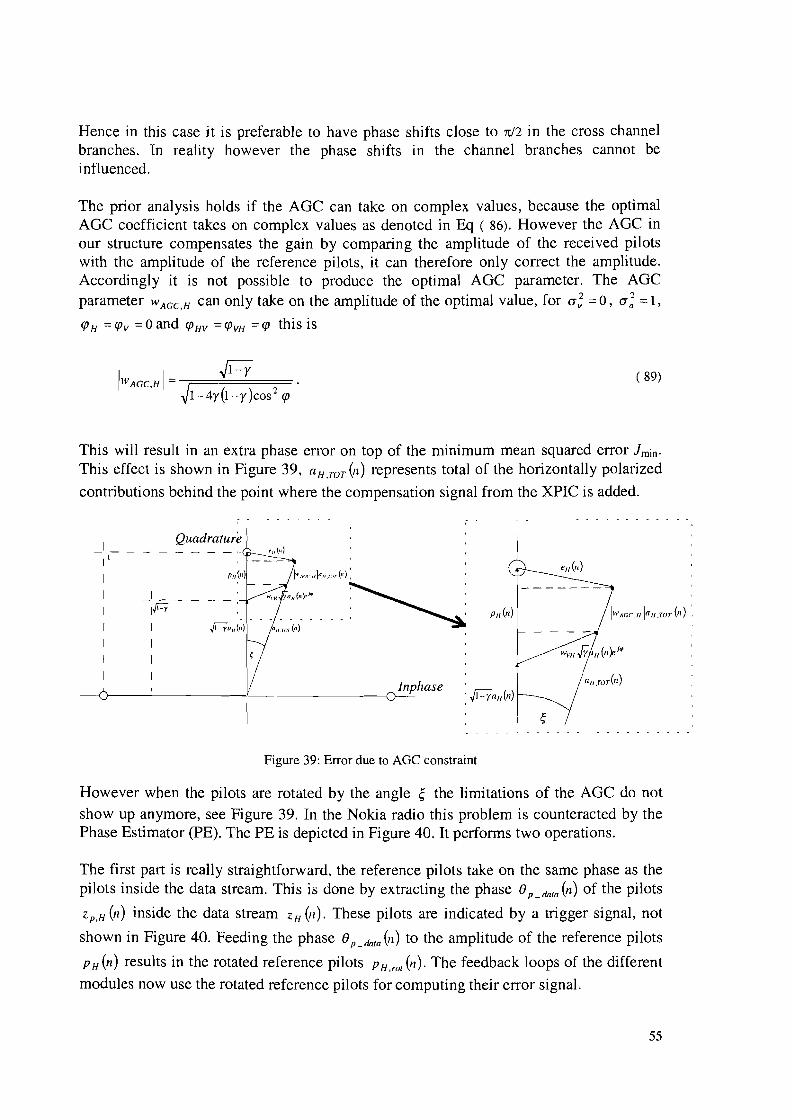
Hence in this case it is preferable to have phase shifts close to n/2 in the cross channelbranches. In reality however the phase shifts in the channel branches cannot beinfluenced.

The prior analysis holds if the AGC can take on complex values, because the optimalAGC coefficient takes on complex values as denoted in Eq ( 86). However the AGC inour structure compensates the gain by comparing the amplitude of the received pilotswith the amplitude of the reference pilots, it can therefore only correct the amplitude.Accordingly it is not possible to produce the optimal AGC parameter. The AGCparameter WAGC,H can only take on the amplitude of the optimal value, for a; =0, a; =1,

qJH =qJv =Oand qJHV =qJVH =qJ this is

I~1-y

W AGC H I = ---,==========. ~1-4Y(I-y)cos2 qJ

( 89)

This will result in an extra phase error on top of the minimum mean squared error imino

This effect is shown in Figure 39, aH,TOT0z) represents total of the horizontally polarized

contributions behind the point where the compensation signal from the XPIC is added.

Quadrature

Inphase-D---~-----I---------~o---'- :ha,,(n)

Figure 39: Error due to AGe constraint

However when the pilots are rotated by the angle ~ the limitations of the AGC do not

show up anymore, see Figure 39. In the Nokia radio this problem is counteracted by thePhase Estimator (PE). The PE is depicted in Figure 40. It performs two operations.

The first part is really straightforward, the reference pilots take on the same phase as thepilots inside the data stream. This is done by extracting the phase 8 p_da/a (n) of the pilots

Z p,H (n) inside the data stream Z H (n). These pilots are indicated by a trigger signal, not

shown in Figure 40. Feeding the phase 8 p _ dat( 01) to the amplitude of the reference pilots

PH(n) results in the rotated reference pilots PH,rot(n). The feedback loops of the different

modules now use the rotated reference pilots for computing their error signal.

55

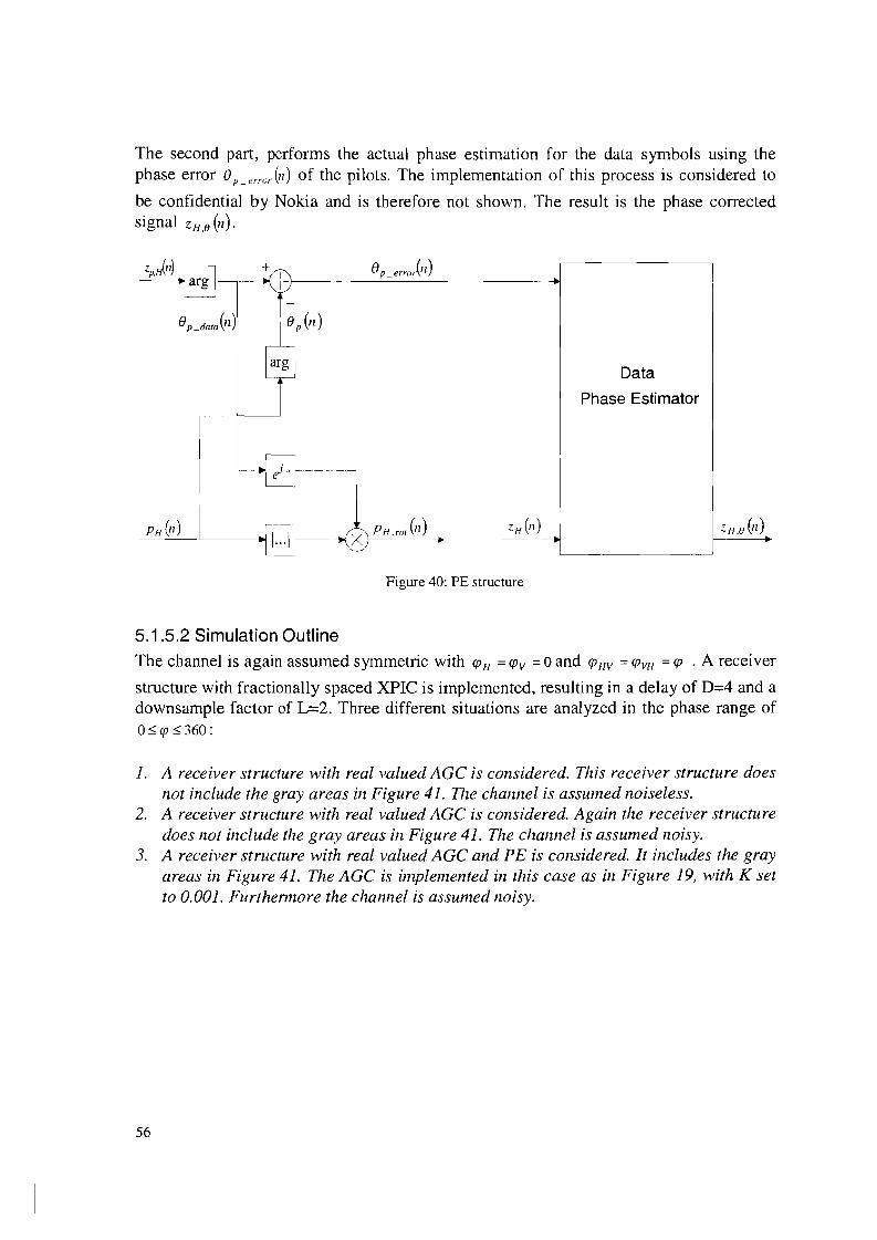
The second part, performs the actual phase estimation for the data symbols using thephase error 8p_error(n) of the pilots. The implementation of this process is considered to

be confidential by Nokia and is therefore not shown. The result is the phase correctedsignal ZH,8 (n).

8p _ errorVl)

Data

Phase Estimator

I~ X PH,rot(n) •---~~JJ -

I

ZH ~,-----I J'H' (n).

Figure 40: PE structure

5.1.5.2 Simulation Outline

The channel is again assumed symmetric with ({JH = ({Jv = 0 and ({JHV = ({JVH = ({J • A receiver

structure with fractionally spaced XPIC is implemented, resulting in a delay of D=4 and adownsample factor of L=:2. Three different situations are analyzed in the phase range ofO~({J ~360:

1. A receiver structure with real valued AGC is considered. This receiver structure doesnot include the gray areas in Figure 41. The channel is assumed noiseless.

2. A receiver structure with real valued AGC is considered. Again the receiver structuredoes not include the gray areas in Figure 41. The channel is assumed noisy.

3. A receiver structure with real valued AGC and PE is considered. It includes the grayareas in Figure 41. The AGC is implemented in this case as in Figure 19, with K setto 0.001. Furthennore the channel is assumed noisy.

56

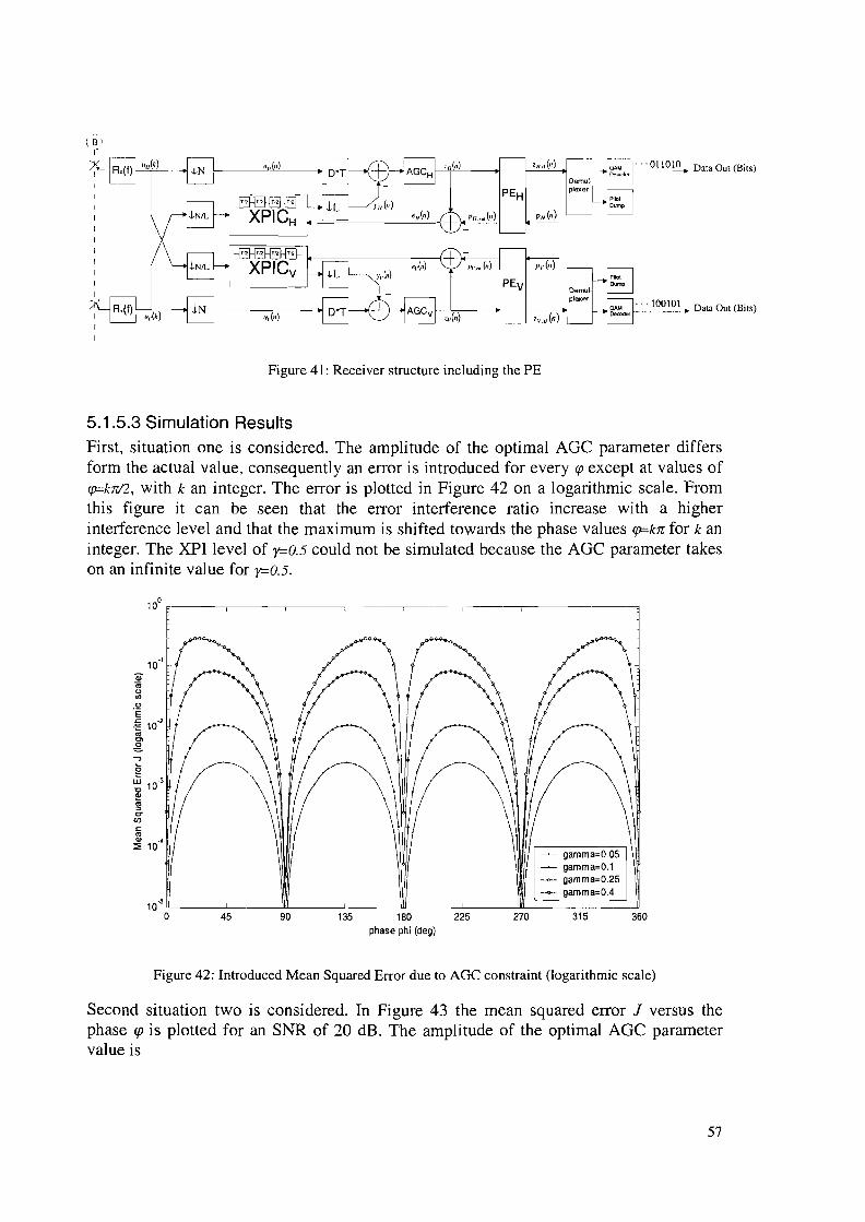
-(B I

r:x

I

II

II

II

I

I

AI

I

I

Figure 41: Receiver structure including the PE

5.1.5.3 Simulation ResultsFirst, situation one is considered. The amplitude of the optimal AGC parameter differsform the actual value, consequently an error is introduced for every qJ except at values ofqFk7rl2, with k an integer. The error is plotted in Figure 42 on a logarithmic scale. Fromthis figure it can be seen that the error interference ratio increase with a higherinterference level and that the maximum is shifted towards the phase values qFkn for k aninteger. The XPI level of y=O.5 could not be simulated because the AGC parameter takeson an infinite value for r=O.5.

360315270135 180 225phase phi (deg)

9045

- gamma=0.05- gamma=O.l- gamma=0.25~ gamma=O.4

10.5 L __--"--- ~ _'_____JlL _"_ L'=~:=L==~

o

Figure 42: Introduced Mean Squared Error due to AGe constraint (logarithmic scale)

Second situation two is considered. In Figure 43 the mean squared error J versus thephase qJ is plotted for an SNR of 20 dB. The amplitude of the optimal AGC parametervalue is

57

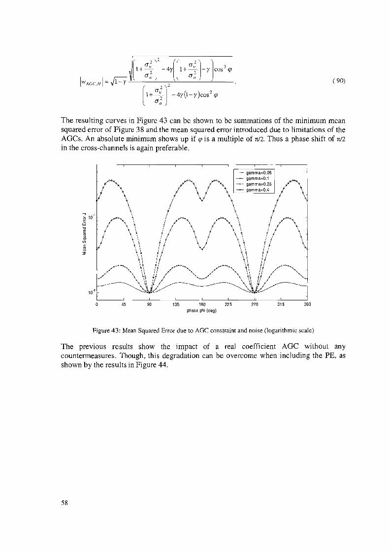
( 90)

The resulting curves in Figure 43 can be shown to be summations of the minimum meansquared error of Figure 38 and the mean squared error introduced due to limitations of theAGCs. An absolute minimum shows up if qJ is a multiple of nl2. Thus a phase shift of nl2

in the cross-channels is again preferable.

- gamma=0.05- gamma=0.1- gamma=0.25- gamma=O.4

...., -1g10W'0l!!'"=>c:T

U)

<:::

'"Q)

:<

o 45 90 135 180 225phase phi (deg)

270 315 360

Figure 43: Mean Squared Error due to AGe constraint and noise (logarithmic scale)

The previous results show the impact of a real coefficient AGC without anycountermeasures. Though, this degradation can be overcome when including the PE, asshown by the results in Figure 44.

58

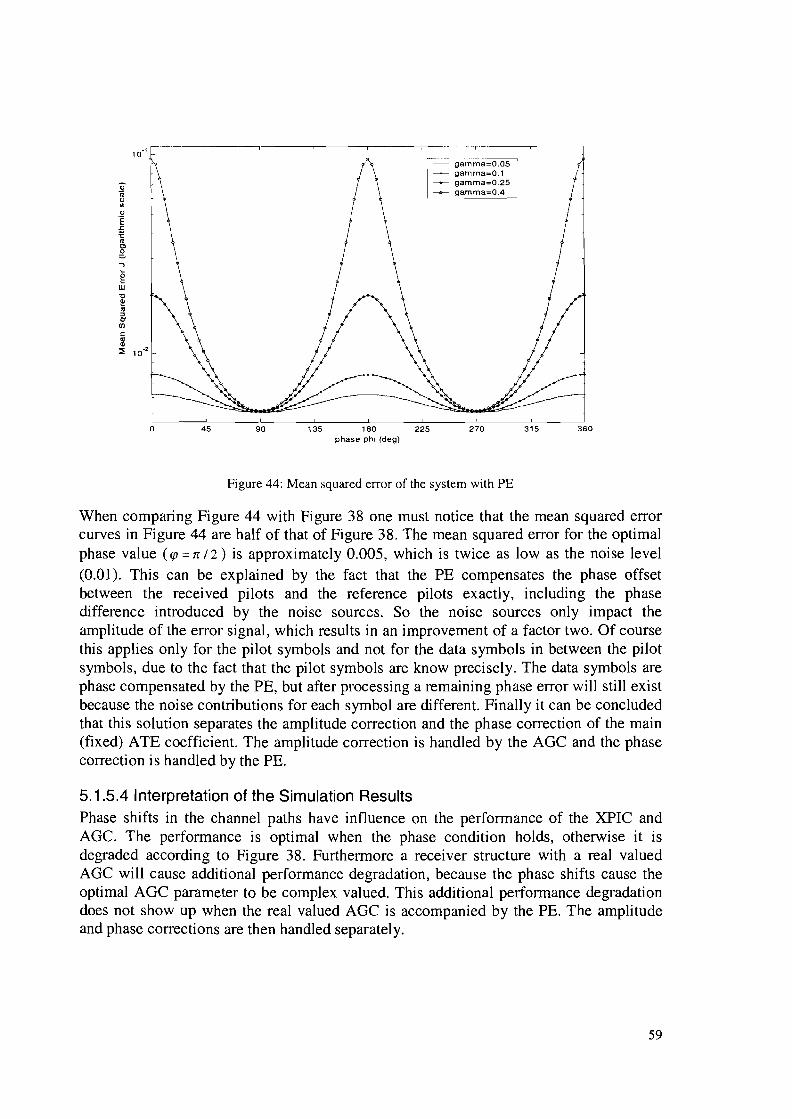
0;­n;".."·E-=.~Clg...,gW"tl~

'":JC­enc:'"<ll

:::!: 10.2

o 45 90 135 160 225phase phi (deg)

- gamma=0.05- gamma=O.1- gamma=O.25___ gamma=O.4

270 315 360

Figure 44: Mean squared error of the system with PE

When comparing Figure 44 with Figure 38 one must notice that the mean squared errorcurves in Figure 44 are half of that of Figure 38. The mean squared error for the optimalphase value (qJ =n /2) is approximately 0.005, which is twice as low as the noise level(0.01). This can be explained by the fact that the PE compensates the phase offsetbetween the received pilots and the reference pilots exactly, including the phasedifference introduced by the noise sources. So the noise sources only impact theamplitude of the error signal, which results in an improvement of a factor two. Of coursethis applies only for the pilot symbols and not for the data symbols in between the pilotsymbols, due to the fact that the pilot symbols are know precisely. The data symbols arephase compensated by the PE, but after processing a remaining phase error will still existbecause the noise contributions for each symbol are different. Finally it can be concludedthat this solution separates the amplitude correction and the phase correction of the main(fixed) ATE coefficient. The amplitude correction is handled by the AGC and the phasecorrection is handled by the PE.

5.1.5.4 Interpretation of the Simulation ResultsPhase shifts in the channel paths have influence on the performance of the XPIC andAGe. The performance is optimal when the phase condition holds, otherwise it isdegraded according to Figure 38. Furthermore a receiver structure with a real valuedAGC will cause additional performance degradation, because the phase shifts cause theoptimal AGC parameter to be complex valued. This additional performance degradationdoes not show up when the real valued AGC is accompanied by the PE. The amplitudeand phase corrections are then handled separately.

59

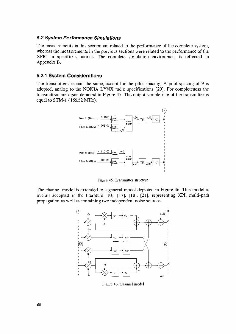
5.2 System Performance Simulations

The measurements in this section are related to the performance of the complete system,whereas the measurements in the previous sections were related to the performance of theXPIC in specific situations. The complete simulation environment is reflected inAppendix B.

5.2.1 System Considerations

The transmitters remain the same, except for the pilot spacing. A pilot spacing of 9 isadopted, analog to the NOKIA LYNX radio specifications [20]. For completeness thetransmitters are again depicted in Figure 45. The output sample rate of the transmitter isequal to STM-l (155.52 MHz).

Data In (Bits) ... 011010

Pilots In (Bits) .. ·001101

Data In (Bits) ···110100

Pilots In (Bits) ... 100101

(AIrI

Figure 45: Transmitter structure

The channel model is extended to a general model depicted in Figure 46. This model isoverall accepted in the literature [10], [17], [18], [21], representing XPI, multi-pathpropagation as well as containing two independent noise sources.

(AIr

I

I

I

I

I

I

'c1D~

:~~II

I

I

I

Figure 46: Channel model

60

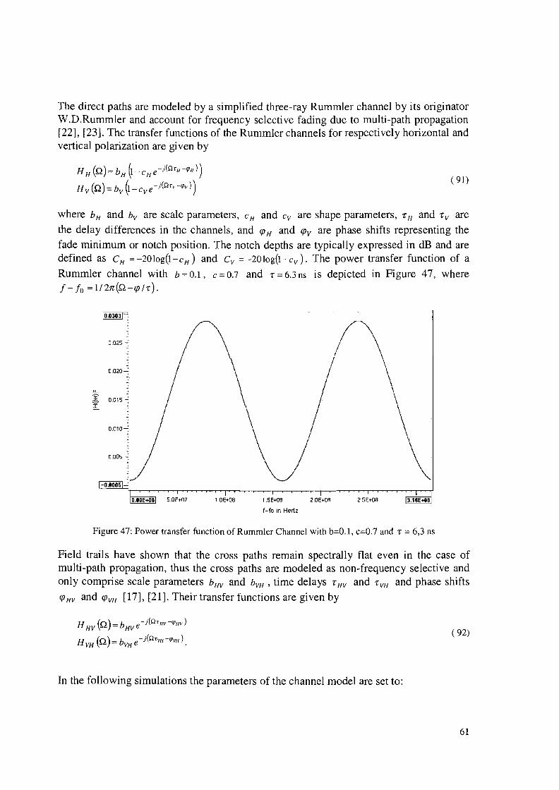
( 91)

The direct paths are modeled by a simplified three-ray RummIer channel by its originatorW.D.Rummler and account for frequency selective fading due to multi-path propagation[22], [23]. The transfer functions of the RummIer channels for respectively horizontal andvertical polarization are given by

H H (Q) = bH (1-cHe-j(~hl/-'PfI))

H v (Q) = bv (1- Cv e - j(QTV-'Pv ) )

where bH and bv are scale parameters, CH and Cv are shape parameters, 7: H and 7:v are

the delay differences in the channels, and qJ Hand qJv are phase shifts representing thefade minimum or notch position. The notch depths are typically expressed in dB and aredefined as C H =-20Iog(1-cH) and Cv =-20Iog(1-cv). The power transfer function of a

RummIer channel with b=O.1, c=O.7 and r=6.3ns is depicted in Figure 47, wheref- fo =l!2n(Q-qJl7:).

0.025 --:

0.020-:

0.010'--:

0.005 ..:

O.OOE+80 5.0E+07 1.0E+08 1.5E+OB

f-fo in Hertz

2.0E+OB 2.5E+08 3.16E-tll8

Figure 47: Power transfer function of Rummier Channel with b=O.l, c=O.7 and r = 6,3 ns

Field trails have shown that the cross paths remain spectrally flat even in the case ofmulti-path propagation, thus the cross paths are modeled as non-frequency selective andonly comprise scale parameters bHV and bVH ' time delays 7: HV and r VH and phase shiftsqJ HV and qJVH [17], [21]. Their transfer functions are given by

H (n)-b e-j(QTl/v-'Pl/v)HV - HV

H (n) - b e - j(QTVI/ -'PVI/ )VH - VH .

In the following simulations the parameters of the channel model are set to:

( 92)

61

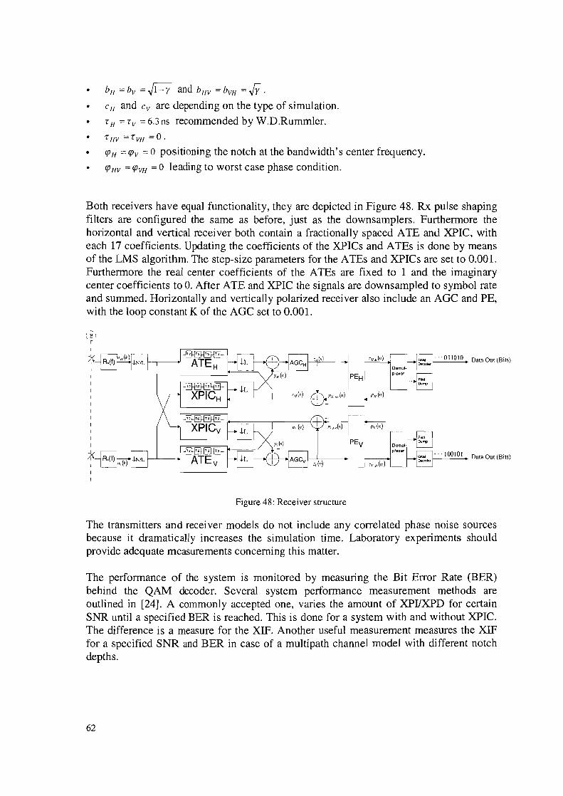
bH = bv = hand bHV = bVH = JY.cHand Cv are depending on the type of simulation.T H =Tv =6.3ns recommended byW.D.Rummler.T HV =TVH = o.({J H =({Jv =0 positioning the notch at the bandwidth's center frequency.

({J HV =({JVH =0 leading to worst case phase condition.

Both receivers have equal functionality, they are depicted in Figure 48. Rx pulse shapingfilters are configured the same as before, just as the downsamplers. Furthermore thehorizontal and vertical receiver both contain a fractionally spaced ATE and XPIC, witheach 17 coefficients. Updating the coefficients of the XPICs and ATEs is done by meansof the LMS algorithm. The step-size parameters for the ATEs and XPICs are set to 0.001.Furthermore the real center coefficients of the ATEs are fixed to 1 and the imaginarycenter coefficients to O. After ATE and XPIC the signals are downsampled to symbol rateand summed. Horizontally and vertically polarized receiver also include an AGC and PE,with the loop constant K of the AGC set to 0.001.

(BIr

+~~PEV

I--=-=::'=-' Data Out (Bits)

.-,-~ Data Out (Bits)

Figure 48: Receiver structure

The transmitters and receiver models do not include any correlated phase noise sourcesbecause it dramatically increases the simulation time. Laboratory experiments shouldprovide adequate measurements concerning this matter.

The performance of the system is monitored by measuring the Bit Error Rate (BER)behind the QAM decoder. Several system performance measurement methods areoutlined in [24]. A commonly accepted one, varies the amount of XPI/XPD for certainSNR until a specified BER is reached. This is done for a system with and without XPIC.The difference is a measure for the XIF. Another useful measurement measures the XIFfor a specified SNR and BER in case of a multipath channel model with different notchdepths.

62

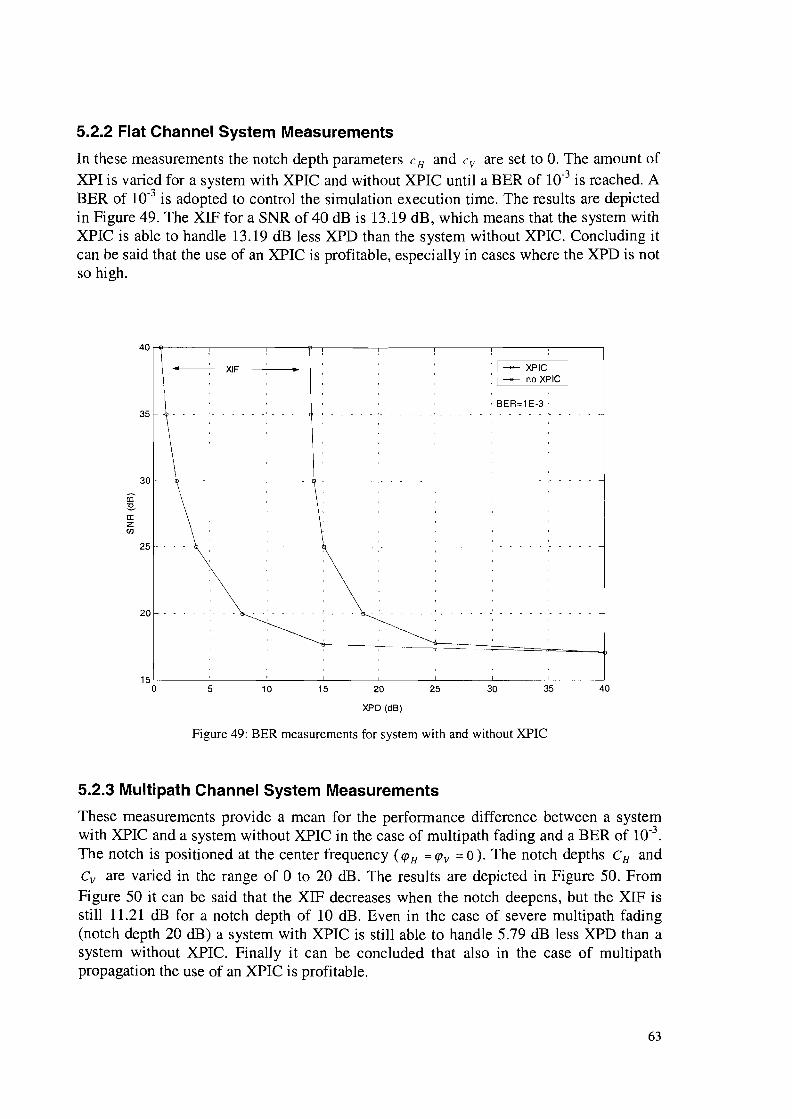
5.2.2 Flat Channel System Measurements

In these measurements the notch depth parameters cHand C v are set to O. The amount ofXPI is varied for a system with XPIC and without XPIC until a BER of 10-3 is reached. ABER of 10-3 is adopted to control the simulation execution time. The results are depictedin Figure 49. The XIF for a SNR of 40 dB is 13.19 dB, which means that the system withXPIC is able to handle 13.19 dB less XPD than the system without XPIC. Concluding itcan be said that the use of an XPIC is profitable, especially in cases where the XPD is notso high.

co~

a:z(f)

..

35

30

25 .

20 ...

XIF • I-e- XPIC I: -e- no XPIC

, BER=1 E-3 '

, ,. . - - - - - - - - - - - - - - -

5 10 15 20

XPD (dB)

25 30 35 40

Figure 49: BER measurements for system with and without XPIC

5.2.3 Multipath Channel System Measurements

These measurements provide a mean for the performance difference between a systemwith XPIC and a system without XPIC in the case of multipath fading and a BER of 10-3

.

The notch is positioned at the center frequency (qJ H =qJv =0). The notch depths CHandCv are varied in the range of 0 to 20 dB. The results are depicted in Figure 50. FromFigure 50 it can be said that the XIF decreases when the notch deepens, but the XIF isstill 11.21 dB for a notch depth of 10 dB. Even in the case of severe multipath fading(notch depth 20 dB) a system with XPIC is still able to handle 5.79 dB less XPD than asystem without XPIC. Finally it can be concluded that also in the case of multipathpropagation the use of an XPIC is profitable.

63

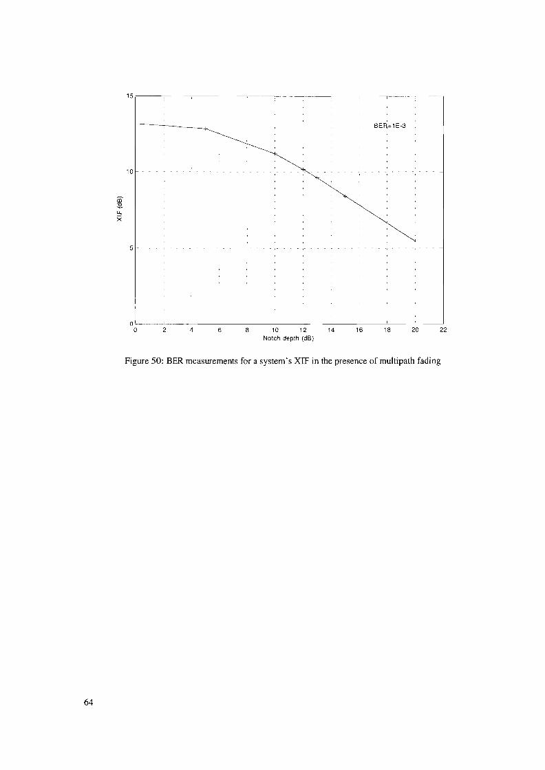
15 ~~~.---~-.-~~-,~---,-----,, ,

BER=1E-3

--

10

iii'~

l.L.

X

5

222018161410 12Notch depth (dB)

86

Io,-'~~---'~~--'---~--'-~~--'-~~---'~~~'---~~-'---~~---'-~~--'-~~---'--~-o 2 4

Figure 50: BER measurements for a system' s XIF in the presence of multipath fading

64

6. Conclusions

In this report several problems relating to the integration of an XPIC into an existingNokia radio architecture have been studied. Results are derived on a simulation basis,supported with theoretical analyses. Detailed description is given of the transmitter,channel, and receiver structures and in specific the functionality of the XPIC and therelated units is treated intensively.

First of all several XPIC and AGC combinations are considered. The best position for theAGC from a simulation point of view as well as from a theoretical point of view is foundto be behind the XPIC. The other AGC locations lead to residual gain errors. Howeverequally well results can be achieved when the AGe's gain correction takes place at eachof the considered positions, if only the error signal of the AGC is derived behind theXPIC. However, this will lead to a smaller loop bandwidth of the AGC, decreasing thetracking capability.

Secondly, the performance of a symbol spaced XPIC is compared to the performance of afractionally spaced XPIC under several types of signal delays. A symbol spaced XIPCand a fractionally spaced XPIC are shown to be both capable of compensating symboldelays. A symbol spaced XPIC is able to handle twice as much symbol delay as afractionally spaced XPIC when both structures have the same amount of taps. On theother hand a fractionally spaced XPIC is able to handle fractional delays withoutperformance loss, whereas a symbol spaced XPIC experiences some difficulties. Thoughwhen a symbol spaced XPIC is combined with a Elastic Storage (ES) it will performequally good, due to the capability of an ES to synchronize data streams. Of course thiscreates the need for an extra module, resulting in a more complex schematic.

Thirdly, the dependency of synchronized transmitters and receivers on the operation ofthe XPIC is considered. It has been pointed out that synchronization of only thetransmitters or the receivers is sufficient to ensure XPIC convergence. A choice betweenonF" of the two possibilities depends on the preferred situation.

A synchronized transmitter side leads to interconnections between the two transmitters, tosynchronize the modulator and up-converter as well as to interconnections between thereceivers, to derive the input of the XPIC. In the receivers less components are neededbecause the signal exchange can be made after the ND converter. A prerequisite is acarrier recovery lock state.

A synchronized receiver leads to interconnections at the receiver side, because down­converters need to be synchronized and the input of the XPIC must be derived, but nointerconnections have to be made at the transmitter side. The XPIC is able to work evenwithout a carrier recovery lock state. However extra components like demodulators,filters, ND converters are needed, because the signal exchange is made at IF level.

65

Fourthly, the influence of phase shifts in the channel paths on the performance of theXPIC is considered. It has been shown that phase shifts in the channel paths influence theperformance of the XPIC and AGC. The performance was shown to be optimal when thephases of the main channel paths and the cross channel paths differ 180 degrees.Furthermore a receiver structure with a real valued AGC will cause additionalperformance degradation, because the phase shifts cause the optimal AGC parameter tobe complex valued. This additional performance degradation does not show up when thereal valued AGC is accompanied by a PE. The amplitude and phase corrections are thenhandled separately.

Finally the integration of an XPIC in a Nokia specific radio system is shown to beprofitable. The performance of the system increases when a channel suffers from XPI,also in the case of multipath propagation.

66

7. Recommendations

I would recommend a receiver structure implemented with a fractionally spaced XPICconsisting of the same number of taps as the ATE. Furthermore I would recommend asynchronized receiver side, due to the fact that it is independent of the carrier lock-instate, and besides it leaves the transmitter side untouched. I consider including extramodules in the path of the XPIC, like demodulators and AID converters of minorsignificance, because the extra costs of those modules are small. I would also recommendto place the AGC behind or at least derive the error signal of the AGC from behind thepoint where the signal from the XPIC is added.

Most probably the XPI contribution will interfere with the slow carrier recovery loop andthe timing recovery loop, therefore the optimal solution might be adding the XPI cancelcontribution of the XPIC in front of the feedback of the slow carrier recovery loop andthe timing recovery loop. This would be behind the receiver's pulse shaping filter. Theeffect of XPI on the functioning of the slow carrier loop and the timing recovery loopshould be made clear and will therefore need to be subjected to investigation in thefuture.

The XPIC depends on the pilot detection block in the receiver, meaning that the XPICdoes not work when the pilots are not detected. This might make it necessary to introduceblind adaptation techniques until the pilots are detected. The dependency of the pilotdetection lock-in state on XPI should be investigated. Investigations at Nokia revealedthe need for these techniques for the ATE. The algorithm used for the blind adaptation inthe ATE is the Godard algorithm or also called the Constant Modulus Algorithm (CMA).

Finally it is good to say that it is known that fractionally spaced adaptive filter structureslike the one presented for the XPIC can lead to tap wandering, increasing the tapcoefficients and maybe causing a register overflow. Deeper investigation of thefractionally spaced XPIC should clarify this and suitable solutions should be presented.Possible solutions for this problem could be the simple tap-leakage algorithm or the morecomplicated algorithm presented by Uyematsu and Sakaniwa.

67

8. List of Abbreviations

AIDADCAGCAPATE

BBBER

CMACC

DADACDFG

ESETSI

FIFOFIR

GSM

lSIIF

LMS

NDA

PDHPE

QAMQPSK

RF

SDHSNRSTM

Analog / DigitalAnalog Digital ConverterAutomatic Gain ControlAlternating PatternAdaptive Transversal Equalizer

BaseBandBit Error Rate

Constant Modulus AlgorithmCo-Channel

Decision AidedDigital Analog ConverterData Flow Graph

Elastic StorageEuropean Telecommunications Standard Institute

First In First OutFinite Impulse Response

Global System for Mobile communication

Inter Symbol InterferenceIntermediate Frequency

Least Mean Square

Non Decision Aided

Plesiochronous Digital HierarchyPhase Estimator

Quadrature Amplitude ModulationQuadrature Phase Shift Keying

Radio Frequency

Synchronous Digital HierarchySignal to Noise RatioSynchronous Transport Module

69

TCM

UMTS

XIFXPDXPIXPIC

70

Trellis Coded Modulation

Universal Mobile Telecommunication System

XPIC Improvement FactorCross Polarization DiscriminationCross Polarization InterferenceCross Polarization Interference Canceller

9. References

[1] I. Henne and P. Thorvaldsen, "Planning of line-of-sight radio relay systems", NeraTelecommunications, Bergen, September 1999, p.99.

[2] LR.A. Bahamonde, J.M.T. Romano and J.C.M. Mota, "On the adaptive filtering forcross-polarization interference canceler", IEEE International TelecommunicationsSymposium 1990, p.317-21.

[3] L. Scarabosio, "Influence of the phase relationship between direct path andinterference path on XPIC performance", IEEE Globecom 1995, Communication forglobal harmony, Vol. 3, p.2017-21.

[4] S. Bregni, "A historical perspective on telecommunications networksynchronization", IEEE Communications Magazine, June 1998, Vol. 36, no. 6, p.158-66.

[5] T.S. Rappaport, "Wireless communications principles and practice", Prentice Hall,New Jersey, 1996, p.270.

[6] S. Haykin, "Adaptive filter theory", Prentice-Hall, New Jersey, 1996.

[7] K. Vogel and K.J. Friederichs, "The benefit of cross-polar co-channel operation indigital radio networks", IEE Proceedings 4th ECRR 1993, Edinburgh, UK, p.167-74.

[8] G. Sebald, G. Filiberti, R. Schmidmaier and S. Bianchi, "A STM-l XPIC-modem for28/30 MHz cochannel applications", IEE Proceedings. 5th ECRR 1996, Bologna, Italy,p.265-71.

[9] B. Lankl, A. Nist, J.A. Nossek and G. Sebald, "Fully digital ATDE's and XPIC's fora STM-l cochannel radio system family", IEEE World prosperity throughcommunications ICC, 1989, Boston, Vol. 2, p.l013-19.

[10] B. Lankl and G. Sebald, "Optimization of XPIC-performance", IEEE Globecom1990, Communications: Connecting the Future, Vol. 2, p.1196-202.

[11] R. Schmidmaier, G. Sebald, K.J. Friederichs, R. Macchi and M. Traverna, "A newcochannel radio system for 28/30 Mhz frequency spacing based on narrow-Band RFbranching concept", IEE Proceedings 5th ECRR 1996, Bologna, Italy, p. 232-37

[12] R.D. Gitlin and S.B. Weinstein, "Fractionally-spaced equalization: an improveddigital transversal equalizer", The Bell System Technical Journal, Vol. 60, No.2,February 1981, p.275-96.

71

[13] R. Schmidmaier, S. Bianchi and E. de Man, "A new single chip QAM-modem forSDH and ATM systems", IEE Proceedings i h ECRR 2000, Dresden, Germany, p. 115­22.

[14] P. Balducci, M. Bolla, L. Rossi and A. Spalvieri, "A new 32 QAM modem fordoubling transmission capacity in 40 MHz channelling plans", IEEE Globecom 1992,Communication for global users, Vol. 3, p.1840-5.

[15] R.D. Gitlin, HC. Meadors and S.B. Weinstein, "The tap-leakage algorithm: Analgorithm for the stable operation of a digitally implemented, fractionally spaced adaptiveequalizer", The Bell System Technical Journal, Vol. 61, No.8, October 1982, p.1817-39.

[16] T. Uyematsu and K. Sakaniwa, "A new tap-adjustment algorithm: an algorithm forthe stable operation of a digitally implemented, fractionally spaced adaptive equalizer",IEEE Globecom 1985, p.1420-3.

[17] M. Biester, E. Douverne, U. Htilsen, K. Ruthemann and W. Zimmer, "Hardwarerealization of an XPIC system/measurement method and results", IEE Proceedings 4th

ECRR 1993, Edinburgh, UK, p.255-60.

[18] K.W. Suh, C.Y. Park, G.Y. Hur and D.Y. Lee, "A powerful 13-tap ATDE and XPICimplemented on one chip for co-channel digital radio systems", IEEE NationalTelesystems Conference 1994, p.201-6.

[19] ETSI DTRffM0401O: High capacity DRRS carrying SDH signals (lxSTM-1) infrequency bands with about 30 MHz channel spacing and using dual polarized (CCDP)operation.

[20] D. Gaschler et al. , "Lynx1b Specification 2.01b", Nokia Networks, DUsseldorf,August 2000.

[21] B. Lankl, J.A. Nossek and G. Sebald, "Cross-polarization interference cancellationin the presence of delay effects", IEEE Communications, ICC 1988, Digital Technology- Spanning the universe, Vol. 3, p. 1355-61.

[22] W.D. RummIer, "A new selective fading model: application to propagation data",The Bell System Technical Journal, Vol. 58, No.5, May-June 1979, p.158-66.

[23] W.D. RummIer, "A multipath channel model for line-of-sight digital radio systems",Bell Telephone Laboratories, Holmdel, New Jersey, USA, IEEE ICC 1978, p.47.5/l-4.

[24] IEC 835-2-11: Method of measurement for digital microwave radio transmissionsystems. -Part 2: Measurements on terrestrial radio relay systems. -Section 11: Cross­polar interference canceller.

72

Appendix A: Timing Sensitivity Simulation Results

10"':

0.5 -:

0.0-:

-0.5 -

-10-

Scatter Diagram of Symbol Spaced XPIC

1.0-:

0.5 c:

-0.5 ..:

-\.0-:

Scatter Diagram of Fractional Spaced XPIC

-1.45 -1.0 -0.5 00

Inphase

05 10 1.44 -1.45 -10 -05 0.0

Inphase

05 10 1.45

Figure 51: Scatter diagrams for situation 1 (t1T=O)

1.0-:

05 ~

0.0.....:

-{l.S ~

-1.O~

Scatter Diagram of Symbol Spaced XPIC

10-:

0.5 -:

-0.5 .:

-1.0-:

Scatter Diagram of Fractional Spaced XPIC

-1.45 -10 -0.5 00

Inphase

05 1.0 1.44 -VII -1.0 -05 00

Inphase

05 10 1.44

Figure 52: Scatter diagrams for situation 2 (t1T=2)

73

~...

1.0--:

0.5 ~

0.0....:.

-0.5 -'

-1.0--

Scatter Diagram

1.0--:

0.5 .,:'

00--:,

-o.5~

-1.0 --: ~

Scaller Diagram Fractional Spaced XPIC

-1.46 -10 -0.5 00

Inphase

05 '0 1.44 -1.45 -10 -0.5 00

lnphase

05 1.0 1.45

Figure 53: Scatter diagrams for situation 3 (.6.T=2%)

Scatter Diagram Scatter Diagram

~ ~

10"":

~ •~ ~ ~.10-

.. : )<

0.5 - . 0.5 -'~

m ~. .~ ~ ~!m.. ~~

! 00- ~ O.o~

CJ

~:6

¥. ...~ ",, .~ .-0.5-' -as -

.~ M.. ., • '~'$-10-: • -:;& -10-J< "E:II

8}i2l : mn--1.46 -, 0 -05 00 05 1.0 1.45 -1.45 -, 0 -0.5 00 05 '0 1.43

lnphase Inphase

Figure 54: Scatter diagrams for situation 4 (.6.T=2Y2)

74

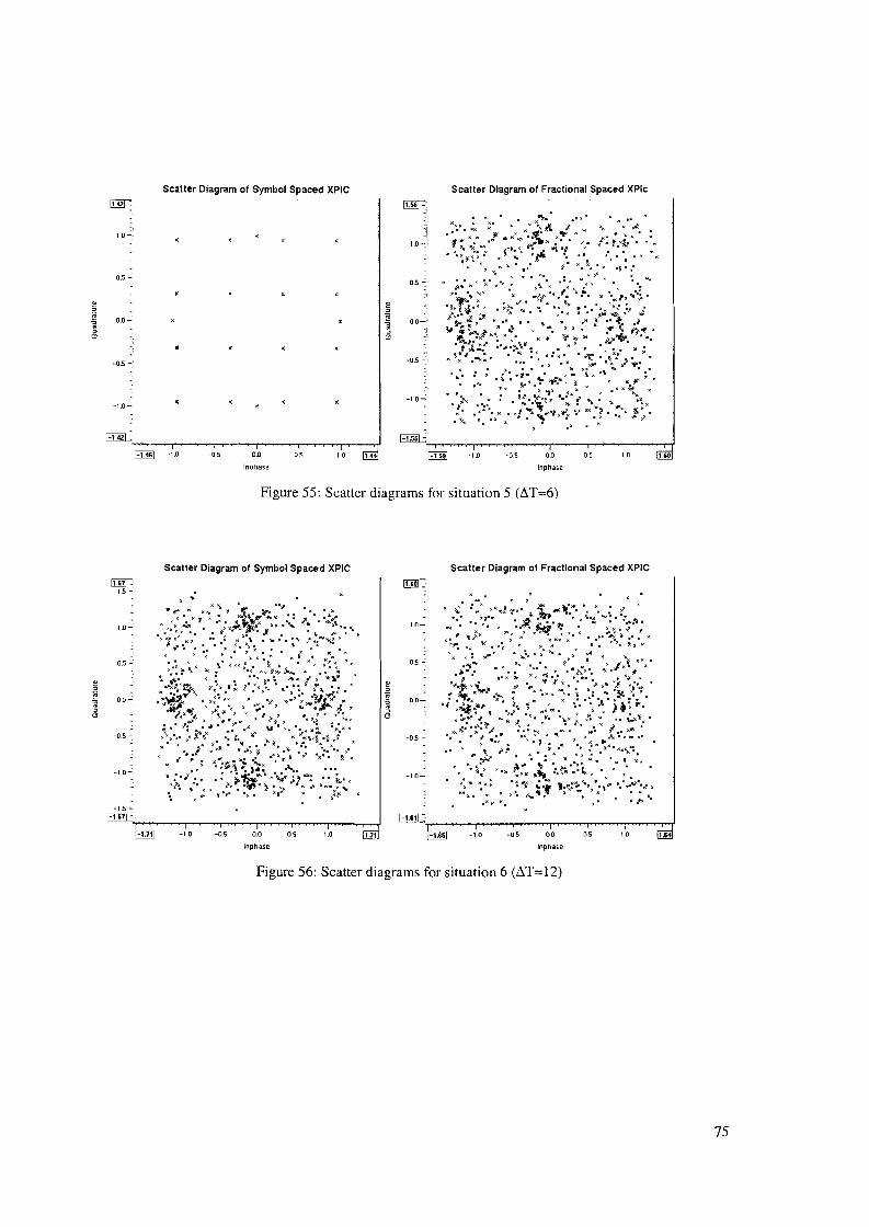
1o~

-0,5 -:'

-1.0-

Scatter Diagram of Symbol Spaced XPIC Scalier Diagram of Fractional Spaced XPlc

-1.46 -1.0 -05 0.0

Inphase

0.5 10 1,44 -1.59 -1.0 -0.5 0.0

lnphase

05 1.0 1.60

Figure 55: Scatter diagrams for situation 5 (~T=6)

Scatter Diagram of Symbol Spaced XPIC[ill'

1.5 ..:

1.0....:

0.5 ~

0.0....:

-10"":

-1.5 -

I'TI1J -,',.~"""'~~"""~-""'~~""'~~""'~~"""r"""~~,....,..,J

Scatter Diagram of Fractional Spaced XPIC

-1.11 -10 -05 0.0

Inphase

05 1.0 1.11 -1.65 -1.0 -05 00

Inphase

05 10 ,..,

Figure 56: Scatter diagrams for situation 6 (~T=12)

75

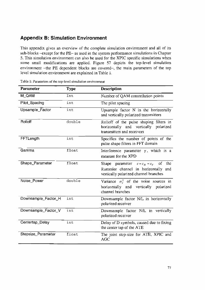
Appendix B: Simulation Environment

This appendix gives an overview of the complete simulation environment and all of itssub-blocks -except for the PE- as used in the system performance simulations in Chapter5. This simulation environment can also be used for the XPIC specific simulations whensome small modifications are applied. Figure 57 depicts the top-level simulationenvironment -the PE dependent blocks are covered-, the main parameters of the toplevel simulation environment are explained in Table 1.

Table 1: Parameters of the top-level simulation environment

Parameter Type

M_QAM Int

Pilot_Spacing int

Upsample_Factor int

Rolloff double

FFTLength int

Gamma float

Shape_Parameter float

Centertap_Delay in t

Stepsize_Parameter f 1 oa t

Description

Number of QAM constellation points

The pilot spacing

Upsample factor N in the horizontallyand vertically polarized transmitters

Rolloff of the pulse shaping filters inhorizontally and vertically polarizedtransmitters and receivers

Specifies the number of points of thepulse shape filters in FFT domain

Interference parameter r, which is ameasure for the XPD

Shape parameter c =C H =Cv of theRummIer channel in horizontally andvertically polarized channel branches

Variance a; of the noise sources inhorizontally and vertically polarizedchannel branches

Downsample factor NIL in horizontallypolarized receiver

Downsample factor NIL in verticallypolarized receiver

Delay of D symbols, caused due to fixingthe center tap of the ATE

The joint step-size for ATE, XPIC andAGC

77

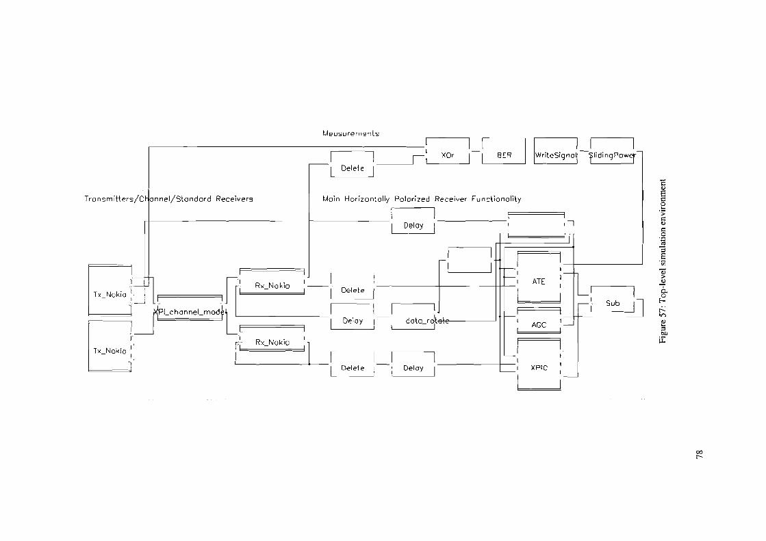
Delele

Meosurements

~---------;::::::::::~--I I l~__~II,---_x_o_r_---,I-~

I'I

XPIC

Delay

Delay

Moin HDrizontolly Polarized Receiver Functionolity

I iF======i I IIx NOKlo : I Jr[,=:=R=x=_=N=o=k=io=d ~~------+-------\--++- ATE I

~~~I ~PI_Ch<Jnnel_modt~ L I I : ~~~_W-~S=Ub=dJ~~ . L I I Delay I doto_roll.~~-------' AGe

I I Rx_Nakio I

Ix NOKiQ I: ['1=.======"1-1

I Delele

TronsmiHers/c onnel/Stondord Receivers

00r--

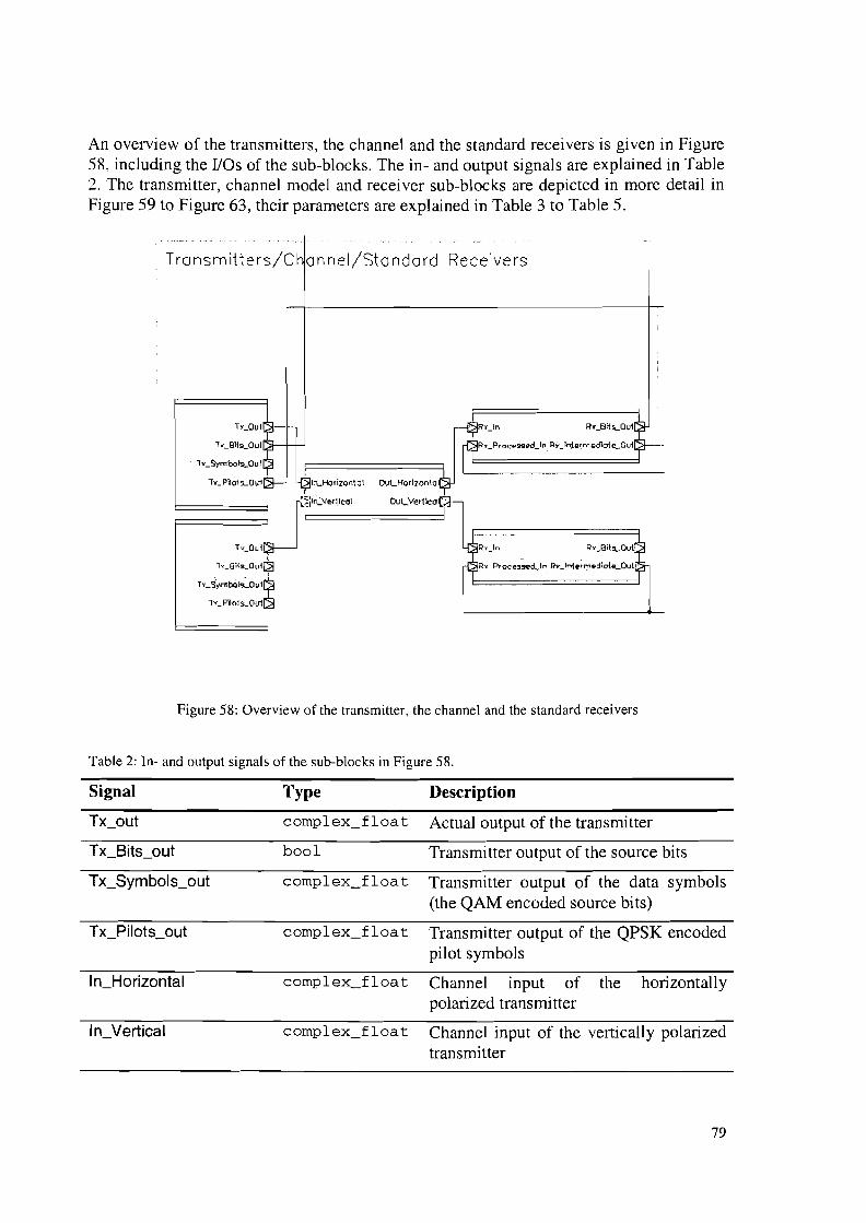
An overview of the transmitters, the channel and the standard receivers is given in Figure58, including the IIOs of the sub-blocks. The in- and output signals are explained in Table2. The transmitter, channel model and receiver sub-blocks are depicted in more detail inFigure 59 to Figure 63, their parameters are explained in Table 3 to Table 5.

Transm iUers/Cha nnel/Sto nda rd Receivers

h_Symbols....Oui

,y_Pilo1,,-Ou1 In.-Horizontol

4~RYJn RY_8fh....Oul~

r~Rv_ProCe39E'(:t..ln Jh"_lnte~rnEodio{'LOui~

Figure 58: Overview of the transmitter, the channel and the standard receivers

Table 2: 1n- and output signals of the sub-blocks in Figure 58.

Signal Type

Tx_out complex_float

Tx_Bits_out bool

Tx_Symbols_out complex_float

Tx_Pilots_out complex_float

In_Horizontal complex_float

In_Vertical complex_float

Description

Actual output of the transmitter

Transmitter output of the source bits

Transmitter output of the data symbols(the QAM encoded source bits)

Transmitter output of the QPSK encodedpilot symbols

Channel input of the horizontallypolarized transmitter

Channel input of the vertically polarizedtransmitter

79

Out_Horizontal

OueVertical

complex_float Channel output for the horizontallypolarized receiver

comp 1ex_fl oa t Channel output for the verticallypolarized receiver

complex_float Receiver input

complex_float Receiver output of the pulse shaped anddownsampled signal

complex_float Receiver input of the processed signal byATE, XPIC, AGC and PE

bool Receiver output of the bits (the QAMdecoded processed signal)

Figure 59: Transmitter architecture

Table 3: Parameters of the transmitter

Parameter

Delay

Upsample_Factor

Cutoff

Rolloff

80

Type

int

int

int

int

double

double

Description

Number of QAM constellation points

The pilot spacing

Delay that enables the horizontally andvertically polarized transmitter to workasynchronious

Upsample factor N in the horizontallyand vertically polarized transmitters

Cutoff frequency of the pulse shapingfilter (normalized to the sample rate)

Rolloff of the pulse shaping filters inhorizontally and vertically polarizedtransmitters and receivers

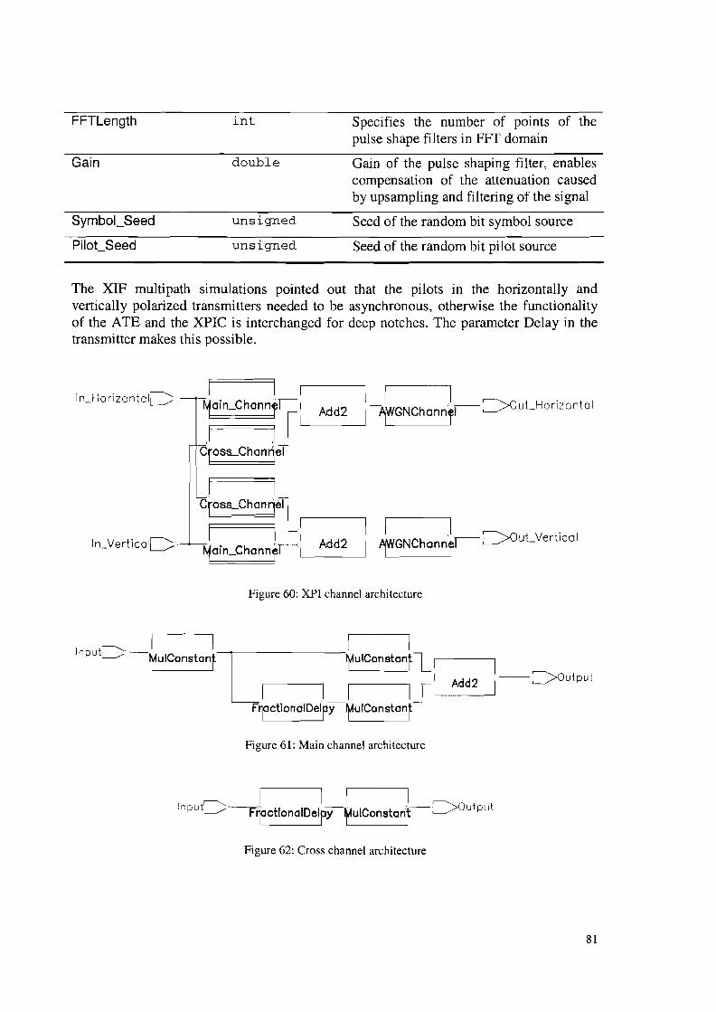
FFTLength

Gain

Symbol_Seed

int

double

unsigned

unsigned

Specifies the number of points of thepulse shape filters in FFf domain

Gain of the pulse shaping filter, enablescompensation of the attenuation causedby upsampling and filtering of the signal

Seed of the random bit symbol source

Seed of the random bit pilot source

The XIF multipath simulations pointed out that the pilots in the horizontally andvertically polarized transmitters needed to be asynchronous, otherwise the functionalityof the ATE and the XPIC is interchanged for deep notches. The parameter Delay in thetransmitter makes this possible.

I 1'---1--1 1~Oin_Chonn1-JI-: Add2 -.AjWGNChannr-'-=>OuLHorizontal

I JCross-Chonn~'

I 1

Cross-chonnrll

II L.r-:-A-d-d2-----,11-...lGNChonn~r-- DOuLVedko I~oin_Chonn1-1-·,---1 I J

Figure 60: XPI channel architecture

InputC._1 I~ .I I~uICon.lanl L, 1_t'Con~on:}I'-- _A_d_d2-----': --=.>Ouiput

F~oetionolDelFY ~uIConston}

Figure 61: Main channel architecture

~ .11 I I ~InputL/··--r'PctlonaIDelpY~Ulconstonr-~Output

Figure 62: Cross channel architecture

81

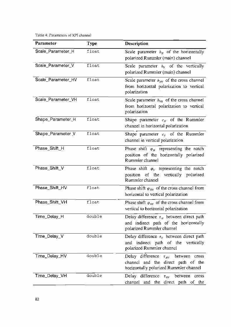
Table 4: Parameters ofXPI channel

Parameter

82

Type

float

float

float

float

float

float

float

float

float

float

double

double

double

double

Description

Scale parameter bH of the horizontallypolarized RummIer (main) channel

Scale parameter bv of the verticallypolarized RummIer (main) channel

Scale parameter bHV of the cross channel

from horizontal polarization to verticalpolarization

Scale parameter bVH of the cross channel

from horizontal polarization to verticalpolarization

Shape parameter C H of the RummIerchannel in horizontal polarization

Shape parameter Cv of the RummIerchannel in vertical polarization

Phase shift <fJ H representing the notch

position of the horizontally polarizedRummIer channel

Phase shift <fJv representing the notch

position of the vertically polarizedRummIer channel

Phase shift <fJ HV of the cross channel fromhorizontal to vertical polarization

Phase shift <fJVH of the cross channel fromvertical to horizontal polarization

Delay difference T H between direct path

and indirect path of the horizontallypolarized RummIer channel

Delay difference Tv between direct path

and indirect path of the verticallypolarized RummIer channel

Delay difference T HV between crosschannel and the direct path of thehorizontally polarized RummIer channel

Delay difference T VH between cross

channel and the direct path of the

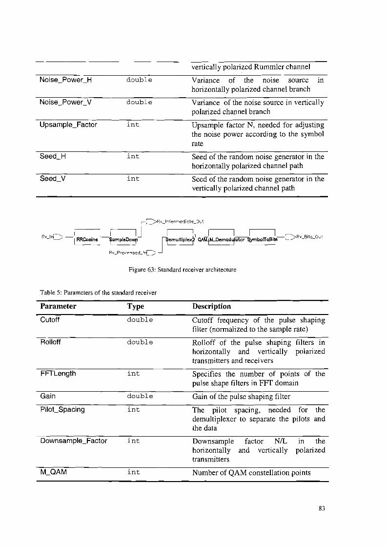
Upsample_Factor

double

double

int

int

int

vertically polarized RummIer channel

Variance of the noise source inhorizontally polarized channel branch

Variance of the noise source in verticallypolarized channel branch

Upsample factor N, needed for adjustingthe noise power according to the symbolrate

Seed of the random noise generator in thehorizontally polarized channel path

Seed of the random noise generator in thevertically polarized channel path

rJRx_lniermediale_Oul

R I~I'--- I I_I iJ I. IL.---,l I I .I_=>RX 8ils Quix_ ''L-/ -I RRCosine I, ~arnpleDowr J~ernu't'P'4 QAMernadjotor ~bolTa8ltr --

Rx_Processed_'C

Figure 63: Standard receiver architecture

Table 5: Parameters of the standard receiver

Parameter

Cutoff

Rolloff

FFTLength

Gain

PiloCSpacing

Downsample_Factor

Type

double

double

int

double

int

int

int

Description

Cutoff frequency of the pulse shapingfilter (normalized to the sample rate)

Rolloff of the pulse shaping filters inhorizontally and vertically polarizedtransmitters and receivers

Specifies the number of points of thepulse shape filters in FFT domain

Gain of the pulse shaping filter

The pilot spacing, needed for thedemultiplexer to separate the pilots andthe data

Downsample factor NIL in thehorizontally and vertically polarizedtransmitters

Number of QAM constellation points

83

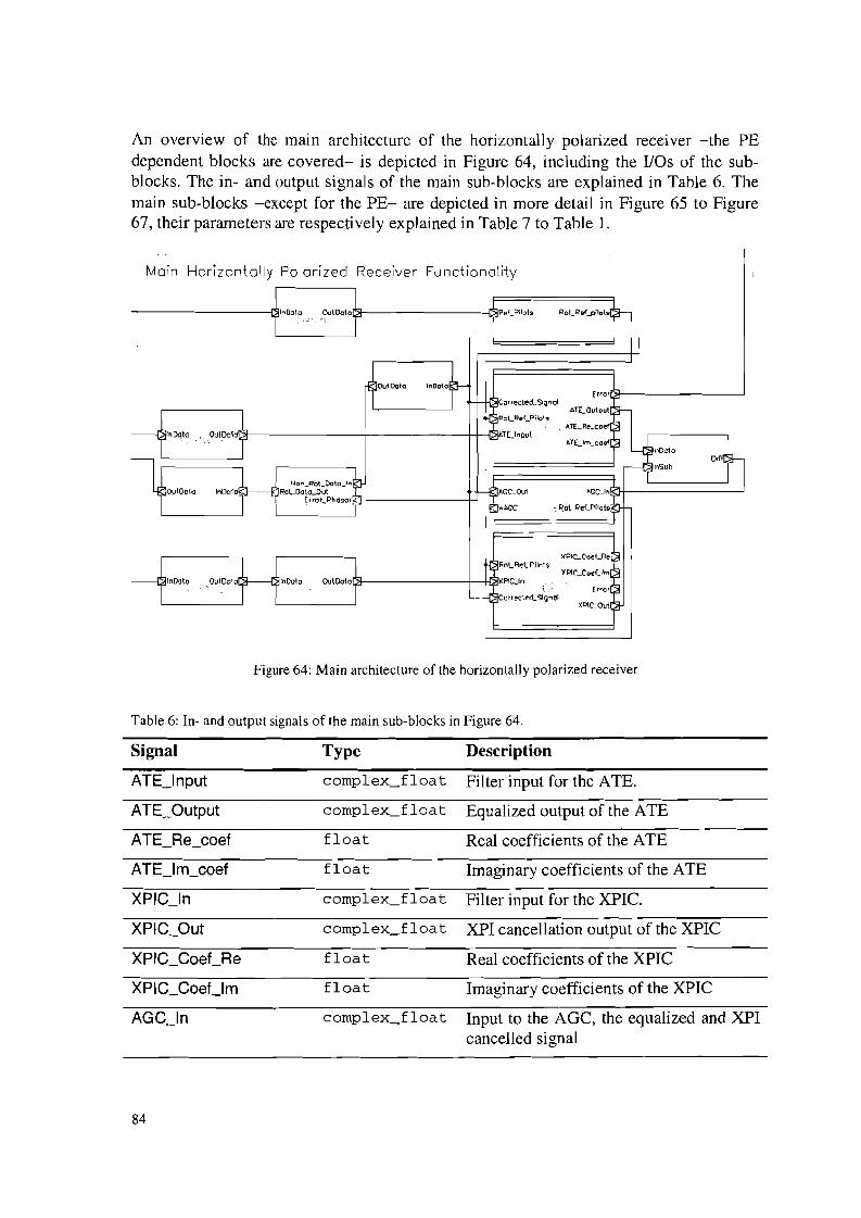
An overview of the main architecture of the horizontally polarized receiver -the PEdependent blocks are covered- is depicted in Figure 64, including the 1I0s of the sub­blocks. The in- and output signals of the main sub-blocks are explained in Table 6. Themain sub-blocks -except for the PE- are depicted in more detail in Figure 65 to Figure67, their parameters are respectively explained in Table 7 to Table 1.

Main Horizontally Polarized Receiver Functionality

f"~· ~,~,+ $Re!_PUOI9 ROI_R..._pnoI9~

I I II

~~OutDoto I"Oo{o~~ ErrQrH~COlrected_Signo'

ATE..Cutput

rt~~..tt F;lOLF;l~'-PilolrATE_Re_coef

--j~noata, . OUID.I. ATUnDutA1L,",_C'oef

~~OUID.l0Olf~nrl ~lnSubWI Non Rot Do\o I,:~ HAGC-OulInOo!ol RoLOoi"a..Cut- AGC-In

T [rror_Phcr~r*.. I! wM;C " ~cL~t!CPilots PiI' I

}('PIC..,CoeeCRe ~

tJ RoLR~f_Pllots

¥P1C'_CoeC'm ~--j~rnDoto .0uloolol~ InD01a OutOoto }{Plc...ln

Err(lr ~~ t1 Co,recte-d_S1qnol

XPIC_Ou! ~

Figure 64: Main architecture of the horizontally polarized receiver

Table 6: In- and output signals of the main sub-blocks in Figure 64.

Signal Type Description

ATE_Input complex_float Filter input for the ATE.

ATE_Output complex_float Equalized output of the ATE

ATE_Re_coef float Real coefficients of the ATE

ATE_lm_coef float Imaginary coefficients of the ATE

XPIC_ln complex_float Filter input for the XPIC.

XPIC_Out complex_float XPI cancellation output of the XPIC

XPIC_CoeCRe float Real coefficients of the XPIC

XPIC_CoeClm float Imaginary coefficients of the XPIC

AGC_ln complex_float Input to the AGC, the equalized and XPIcancelled signal

84

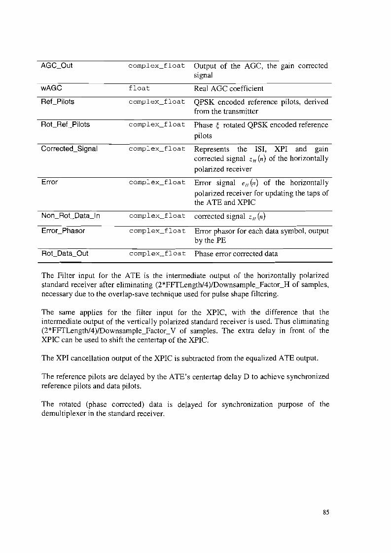
wAGC

ReCPilots

Corrected_Signal

Error

RoCData_Out

complex_float Output of the AGC, the gam correctedsignal

float Real AGC coefficient

complex_float QPSK encoded reference pilots, derivedfrom the transmitter

complex_float Phase ~ rotated QPSK encoded reference

pilots

complex_float Represents the lSI, XPI and gaincorrected signal ZH (n) of the horizontallypolarized receiver

complex_float Error signal eH 01) of the horizontallypolarized receiver for updating the taps ofthe ATE and XPIC

complex_float corrected signal ZH 01)

complex_float Error phasor for each data symbol, outputby the PE

complex_float Phase error corrected data

The Filter input for the ATE is the intermediate output of the horizontally polarizedstandard receiver after eliminating (2*FFTLength/4)/Downsample_FactocH of samples,necessary due to the overlap-save technique used for pulse shape filtering.

The same applies for the filter input for the XPIC, with the difference that theintermediate output of the vertically polarized standard receiver is used. Thus eliminating(2*FFTLength/4)/Downsample_FactocV of samples. The extra delay in front of theXPIC can be used to shift the centertap of the XPIC.

The XPI cancellation output of the XPIC is subtracted from the equalized ATE output.

The reference pilots are delayed by the ATE's centertap delay D to achieve synchronizedreference pilots and data pilots.

The rotated (phase corrected) data is delayed for synchronization purpose of thedemultiplexer in the standard receiver.

85

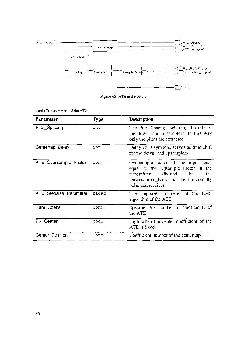
ATUnputC ------ §ATE_Output-----1 ATE_ReJoef

~r I Irl~_E_q_u_ol_iz_er~___________ ATE_1m_coer

I Constant I

I I I I I I I_"got Ref PilotsI Delay I ISampleUp I ~ampleDOW~-L--_S_Ub_---.J:--.·.. Cor~ect~d_Signal

'---------------JError

Figure 65: ATE architecture

Table 7: Parameters of the ATE

Parameter Type

Pilot_Spacing in t

Centertap_Delay int

ATE_Oversample_Factor long

ATE_Stepsize_Parameter float

Num_Coeffs long

Fix_Center bool

CentecPosition long

86

Description

The Pilot Spacing, selecting the rate ofthe down- and upsamplers. In this wayonly the pilots are extracted

Delay of D symbols, serves as time shiftfor the down- and upsamplers

Oversample factor of the input data,equal to the Upsample_Factor in thetransmitter divided by theDownsample_Factor in the horizontallypolarized receiver

The step-size parameter of the LMSalgori thm of the ATE

Specifies the number of coefficients ofthe ATE

High when the center coefficient of theATE is fixed

Coefficient number of the center tap

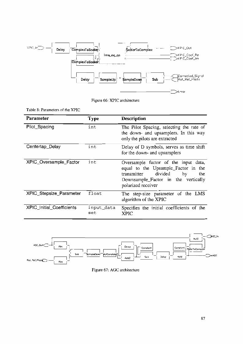
XPIC I r----- I I_I IILI Is-I I ~XPIC 0 \- nl-...---' -L-I_D_e_laY-----'1 CorPleXToSc~ktt::I~larToComgl~ex-;-----~ - u

I ,II]; Ims...e<f_qc :-----'======='---------ES~~:g=g~:;=~~

Sub

=>Error

Figure 66: XPIC architecture

Table 8: Parameters of the XPIC

Parameter

PiloCSpacing

Centertap_Delay

XPIC_Oversample_Factor

XPIC_Stepsize_Parameter

XPI C_I nitial_Coefficients

Type

int

int

int

float

input_dataset

Description

The Pilot Spacing, selecting the rate ofthe down- and upsamplers. In this wayonly the pilots are extracted

Delay of D symbols, serves as time shiftfor the down- and upsamplers

Oversample factor of the input data,equal to the Upsample_Factor in thetransmitter divided by theDownsample_Factor in the verticallypolarized receiver

The step-size parameter of the LMSalgorithm of the XPIC

Specifies the initial coefficients of theXPIC

Figure 67: AGC architecture

87

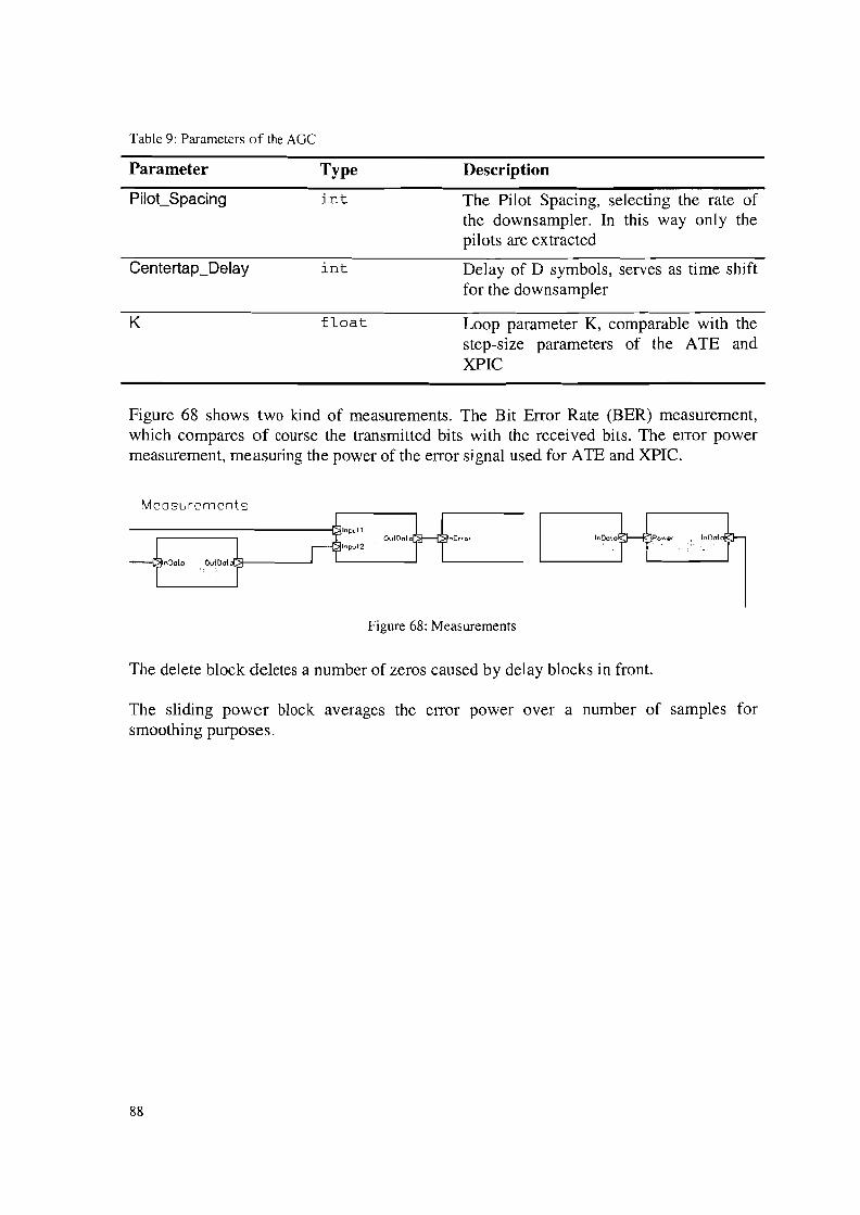
Table 9: Parameters of the AGe

Parameter

PiloCSpacing

Centertap_Delay

K

Type

int

int

float

Description

The Pilot Spacing, selecting the rate ofthe downsampler. In this way only thepilots are extracted

Delay of D symbols, serves as time shiftfor the downsampler

Loop parameter K, comparable with thestep-size parameters of the ATE andXPIC

Figure 68 shows two kind of measurements. The Bit Error Rate (BER) measurement,which compares of course the transmitted bits with the received bits. The error powermeasurement, measuring the power of the error signal used for ATE and XPIC.

Measurements

Input 1

H 3JnErr o l

~1"put2OutOoto

~---t~lnOolo OutDo\o

InDo{o

Figure 68: Measurements

The delete block deletes a number of zeros caused by delay blocks in front.

The sliding power block averages the error power over a number of samples forsmoothing purposes.

88