Eindhoven University of Technology

MASTER

Warranty repairs

production planning and order acceptance

van Kesteren, S.W.J.

Award date:2008

DisclaimerThis document contains a student thesis (bachelor's or master's), as authored by a student at Eindhoven University of Technology. Studenttheses are made available in the TU/e repository upon obtaining the required degree. The grade received is not published on the documentas presented in the repository. The required complexity or quality of research of student theses may vary by program, and the requiredminimum study period may vary in duration.

General rightsCopyright and moral rights for the publications made accessible in the public portal are retained by the authors and/or other copyright ownersand it is a condition of accessing publications that users recognise and abide by the legal requirements associated with these rights.

• Users may download and print one copy of any publication from the public portal for the purpose of private study or research. • You may not further distribute the material or use it for any profit-making activity or commercial gain

Take down policyIf you believe that this document breaches copyright please contact us providing details, and we will remove access to the work immediatelyand investigate your claim.

Download date: 18. Jul. 2018

Eindhoven, August 2008

Warranty repairs:

Production planning andOrder acceptance

bySebastiaan WJ. van Kesteren

BSc Industrial Engineering and Management Science - TV/e 2005Student identity number 0532781

in partial fulfilment of the requirements for the degree of

Master of Sciencein Operations Management and Logistics

Supervisors:Dr.ir. AJ.D. Lambert, TV/e, AWdr.ir. S.D.P. Flapper, TV/e, OPAC

TUE. Department Technology Management.Series Master Theses Operations Management and Logistics

ARW20080ML

Subject headings: production planning, warranty repairs, order acceptance

2

Preface

My Master Thesis project is finished. It has been a very educational experience, not only withrespect to theory, but even more so with respect to the more practical side of such a large project. It, attimes, has been very enjoyable and at other times, a little frustrating. Overall I look back at a wellspent time period, which could have never turned out this way without the assistance, guidance andhelp of others.

First I would like to thank my supervisors at RICOLEC B.V. for letting me conduct thisproject at their company and supporting me during the project. I would like to thank Mr. Voorbergenfor his comments, ideas and input in the project and his support during the day-to-day work. Mr.Hoornweg is also due thanks for his critical comments and suggestions. Lastly I would like to thankthe repairmen for answering all questions and Mr. Kalff for providing with the as much of thenecessary information as possible.

Secondly lowe thanks to my supervisors at the TV/e. My fist supervisor, Mr. Lambert,deserves credit for his support, ideas and comments both with regard to the content as well as the formof this report. Next to this I would like to thank my second supervisor, Mr. Flapper, for taking his timereading my reports and his valuable comments.

Lastly I would like to thank my family and friends for supporting me and listening to my, notalways cheerful, monologues on the project. Special thanks in this regard are due to my girlfriend whodeserves praise for her patience and the provision of the necessary distraction when it was mostneeded.

3

SUrTlmary

In recent years we have seen an increase in both the number of consumer electronic productsper household and the diversity in these products and a decrease in the price of these products. On theother hand the responsibilities of producers for their products have been enlarged in most majoreconomies as for instance the E.U. Together with lengthening periods of warranty coverage offeredfor marketing reasons this has led to increasing numbers of warranty claims and corresponding returnsof products.

Companies differ in the manner they have chosen to handle this situation. Some companies,to avoid the large uncertainty with respect to returns, have outsourced the lucrative repair ofexpensive products and reimburse the purchasing price or a similar product for all cheaper products.However other companies, among which the company at which this case study was done, have chosento keep the repair in their own hands. This leads to a complicated control situation of the returnedproducts due to the diversity and unpredictability of the flow of products that might or might not beworthwhile to repair. On the other hand companies by doing this, beside the possible economicattractiveness, are enabled to get insight in the quality of their products and use the gatheredknowledge in the development of new products and product support features and prevent fraud withthe returns.

Each claim can be settled by multiple means, either by repairing the specific product, bydistributing a new product or by reimbursing the submitter financially. However a claim has to besettled within a specific period, if not the only open option is to financially reimburse the claim.

This leaves the possibility to select the most lucrative part of the products for repair availableto utilize the available capacity for repair, leaving other products unrepaired. However then nothing isknown, with respect to quality, on the products not repaired. To obtain some knowledge theseproducts can be tested. Also the repair of products is complicated due to the necessity of spare partsfor repairs which might not be available. To obtain these parts cannibalization of other products canbe applied.

Processing the stream of warranty claims therefore requires more then just the decision whatto repair. In this report we have looked at all decisions in the process, being whether to repair aproduct, whether to test it, whether to cannibalize it and whether to settle the claim by replacement ofthe product or financial reimbursement. The decisions were looked at in different detail.

For the decision whether to repair four different redesigns were made focusing on thequestions how to select the right products for repair and the right amount of products. Analysisrevealed the type of failures, capacity utilization and throughput times for repair. These results andinformation available on the returns from a pre-sale test on a product type were taken as a base for theredesigns. The dilemma with respect to production control consisted of achieving high utilizationrates without repairing products too late.

First the present production control system was formalized and extensions were consideredwith respect to order acceptance and stock keeping. The order acceptance undertaken when productsarrive, thus the determination what to repair, was linked explicitly to the capacity available to repairproducts by means of the Work In Process. This redesign was extended with priority rules in whichsome customers receive priority depending on the number of days available for their repair. Thisbased on differences in the maximum throughput time allowed for the different submitters.

This link was extended with a hard upper boundary in the second redesign, in line withCONWIP production control theory (Hopp and Spearman, 2000).

The third redesign modifies the order acceptance function into a two phase decision systemwith little costs for the second final decision on what to repair which is taken when a repairman takesthe product. In this system the first decision to repair is, when workload exceeds a limit, reevaluatedto come to a final decision to repair or not.

4

Finally the fourth redesign considers individual product stock keeping instead of the batchesused in the first redesigns. This redesign was not fully developed, but only conceptually discussed.

The first three redesigns were compared by means of simulation varying among others thenumber of returns, their value and the number of days allowed for processing. The fourth redesignwas compared to the other redesigns based on achievable upper limits.

Results indicate that under current constraints all redesigns can lead to close to optimalperformance; because constraints with respect to the maximum throughput times are not stringent, thedilemma can therefore easily be solved by stocking products in the Work In Process. Decreasing themaximum throughput time for products, both redesign 2 and 3 outperform redesign 1, both with andwithout priority rules, because these redesigns prevent products from being repaired too late. Thepriority rule does improve results for redesign 1 compared to the situation without priority rules,however the results attained by redesign 2 and 3 are still higher in these situations. Under theconsidered practical relevant circumstances no significant difference was observed between redesign2 and 3. However, considering extreme variations on both the supply and demand side redesign 3 isexpected to be more robust against those changes. This is also evident in simulations with one daymaximum throughput time, in which redesign 3 outperforms redesign 2. The performance of redesign3 in terms of the maximal attainable value declines slightly with decreasing capacity but remainsabove 89% of the upper limit on the attainable value. Because of the high performance of this, and theother redesigns, and the necessary handling of products, it is concluded that stock keeping of productsindividually and an associated picking of products as proposed in redesign 4 is not expected to lead tolarge increases in performance.

With respect to literature these results indicate that extending the order acceptance decisioninto a two phase decision procedures with little to no cost for the second decision will only lead tobetter results when capacity is highly utilized and throughput times are stringent. This is in line withconclusions drawn on other extensions of the order acceptance function (Ten Kate, 1994) (Wester etai, 1992). Also the possible use of a maximum inventory level for the Work In Process in situationswith varying product value is shown to yield better results than the same policy without a maximuminventory level. However in order to back and generalize these conclusions the impact of a hard upperboundary for the Work In Process on performance first needs to be tested under different arrivaldistributions and different cost functions for late repairs as well as different costs, in time and money,for the second decision.

With respect to the decision whether to test a product when it is not repaired a procedure wasdeveloped to obtain insight in the failure behavior of not to be repaired products. The proceduredetermines the correct number of tests on not repaired products for a given precision interval andconfidence level. It is shown that this number, when confidence levels of 85% and a precisionintervals widths of 0,20 are used, will be around 20 to 30 products. To achieve fast results the firstarriving products should be tested. However this limits the statistical value of the tests due to the biasthat might be present in this not random sample of the total returns.

Cannibalization is used extensively by RICOLEC. However an extensive policy to determinewhich products should be cannibalized is not developed. This because the requirements with respectto data are large and costly to gather, whilst the revenues of a comprehensive system are small sinceinvestments in spare parts is small. It is therefore not economically attractive for RICOLEC todevelop such a system. A very simple rule governing the decision whether to stock a product forcannibalization was developed. This rule can serve as a simple heuristic to decide which products tostock for cannibalization.

Finally for the decision whether to replace a product or reimburse the submitter financially asimple heuristic was developed based on the costs for replacement and reimbursement. However thisheuristic does not take into account the preferences of submitters, nor the physical possibility toreplace a product, both of which are leading in the final decision and will therefore not be of practicaluse to RICOLEC.

5

Table of ContentsPreface 3

Summary 4

Table of Contents 6

1. Introduction 9

1.1. Warranty returns in the consumer electronics industry 9

1.2. Company description 10

1.3. Report structure 10

2. Research & problem definition 11

2.1. The problem as perceived by RICOLEC 11

2.2. The research framework 11

2.3. Preliminary analysis: The return process described 12

2.4. Preliminary analysis: decision options 14

2.5. Detailed problem description & research questions 16

2.6. Relationship to the academic literature 18

3. Literature study 19

3.1. Warranties 19

3.2. Product failure & failure classification 20

3.3. Warranty returns, product quality & failure 20

3.4. IRIS-classification warranty sampling 22

3.5 Order acceptance & scheduling 23

3.6. Cannibalization & inventory management of spare parts 26

3.7. Conclusion 27

4. Detailed analysis of the current situation 28

4.1. Magnitude and composition of the warranty return flow 28

4.2. Division over the settlement/processing options 30

4.3. Capacity, tasks & performance 32

4.4. Product group failure behavior 35

4.5. Spare part inventory management. 38

4.6. Conclusion 38

5. Outline Redesign 40

6. Repair or not? Redesign 1: repair selection & throughput time control .42

6.1. Redesign 1: Rationale 42

6.2. Redesign 1: Throughput time regulation 42

6.3. Redesign 1: What to repair?: Profitability of repair.. .44

6.4. Redesign 1: Synthesis 45

6.5. Redesign Ib: Priority rules 45

6.6. Redesign 1: Practical implications 46

7. Repair or not?, Redesign 2: Maximum WIP level extension 48

6

7.1. Redesign 2: Rationale 48

7.2. Redesign 2: WIPleve1 control with WIPcap 48

7.3. Redesign 2: Practical implications 48

8. Repair or not?, Redesign 3: Final decision at the repairman .49

8.1. Redesign 3: Rationale 49

8.2. Redesign 3: WIP control mechanism 49

8.3. Redesign 3: practical implications 50

9. Repair or not?, Redesign 4: Individual product scheduling 52

9.1. Redesign 4: Rationale 52

9.2. WIP processing: Individual product access & priority 52

9.3. Redesign 4: practical implications 54

10. Testing products 55

10.1. Why testing products 55

10.2. How many products to test. 55

10.3. Capacity needed for testing 56

11. Cannibalize & replace/reimburse 57

11.1. Stock to cannibalize or sell second hand? 57

11.2. Replace or reimburse? 58

12. Simulation of the repair process 59

12.1. Parameters of interest 59

12.2. Constant parameters 61

12.3. Performance measures 61

12.4. Simulation engine and created models 62

12.5. Model validation 62

12.6. Simulation settings 62

13. Design 1 to 3: results & conclusion 64

13.1. Maximal performance: an upper boundary 64

13.2. Redesign 1 64

13.3. Redesign 2 68

13.4. Redesign 3 69

13.5. Redesign 1 to 3: A conclusion 70

14. Redesign 1 to 3: results for 1 day maximum throughput time 72

14.1. Simulation settings & performance evaluation 72

14.2. Results for redesign 1 to 3 72

15. Decreasing capacity: redesign 3, results 74

15.1. Capacity: the influence of a decrease in capacity 74

16. Design 4: results 75

16.1. Redesign 4: expected benefits 75

17. Recommendations 77

7

17.1. Insight in the failure of not repaired products 77

17.2 Processing of warranty retums 77

18. Conclusion on the contribution to academic literature 79

18.1. Contribution to the academic literature 79

References 80

Appendix 83

8

1. Introduction

The topic of this project is the processing of warranty returns at a trading company inconsumer electronics. Here we will shortly address the developments with respect to warranty returnsin this specific industry and the different ways of handling these returns in the industry. After this wewill give a description of the company at which this project was carried out. Lastly we will discuss thestructure of the report.

1.1. Warranty returns in the consumer electronics industry

1. 1. 1. Warranty: Increasing numbersTraditionally consumer electronics are accompanied with a warranty with which producers

take responsibility for the functioning of the product in the first years after purchase. During morerecent years the warranty period also has become a marketing instrument in that warranty periods arelengthened to persuade customers into buying a product. Also governments, for instance the EuropeanUnion, have accepted legislation which places more responsibility for the functioning of a product onthe producer/importer (eg. EU (2002)). Warranty on consumer electronics generally demands theproducer to supply the consumer with a new functioning product or give him his money back.

On the other hand, in the last decades the number of electronic devices per consumer has risensteeply (Widmer et at, 2005). Numerous new products and product types have been developed atincreasing speed and others have become more affordable due to advances in technology. Thesedevelopments have also made consumer electronic devices more complex incorporating more andmore functionality in one product (Brombacher et at, 2005).

These developments have given rise to a large increase in the number of products governedby warranty in the field and, although it is widely assumed that the reliability of products hasincreased over the years, to a large number of warranty claims filed.

1. 1.2. Warranty return repair: decreasing profitability, increasing complexityIn the past, consumer electronics could be regarded like capital goods in industry, highly

valuable, and were repaired if physically possible. However the repair of consumer electronics is notthat obvious anymore. The increase in complexity of products and the diversification of products hasmade it harder to find the failure in a product, since the number of possible failures has increased, andcorrect it. The decrease in price has made the repair less profitable. Besides this the increasing speedwith which new product types are developed and the relatively small, and unpredictable, number ofreturns per product type, which mostly require slightly different repairs, have increased the skillneeded for the repair of products and consequently the labor costs.

On the other hand the increase in complexity has made it more difficult for users to use aproduct. This has led to an increase in warranty claims for products that are not actually defect, butthe consumer does not know how to use the product.

1. 1.3. Warranty returns: reverse logisticsThe developments discussed above have created a large flow of consumer electronic devices

back to producers, a flow of which the size and composition is largely unknown and hard to predict.This flow is handled differently by different producers. Some producers have at the moment chosen tooutsource the repair of the products still economically profitable to repair to specialized repaircompanies and to reimburse the purchasing price for other products. This option saves companiesfrom the duties of performing repairs and all the uncertainty related to the flow of returns. On theother hands it also makes it more difficult to prevent fraud in repairs, filter out easily repairableproducts, consumer faults and it complicates the analysis of the quality of products based on thereceived warranty returns.

Other companies, as the company at which this project is done, have chosen to repair productsthemselves in order to have control over their products and their claims. However this choice requires

9

these companies to process these products and it obliges them to choose which products are repairedand for which either a replacement or a financial reimbursement needs to be made.

1.2. Company descriptionThe used brand names are made-up and mask the real brand names.The company at which this project was conducted, RICOLEC B.V., is now a trading

company employing 25 people. However the company started as a retail shop in music records andelectronics, which formed the foundation of what the company has become today. Over the years,RICOLEC has evolved from a retail business to wholesaler and on to an import company in theelectronic consumer goods branch with a growing turnover that measured around €20 million in 2006.

From the 70's onwards RICOLEC has imported electronic consumer goods from Japan,Korea, Taiwan and China. Over time the sold product assortment has evolved into a large product andbrand portfolio, with brands that stand strongly in the market, and are being sold through well-knownchannels. Next to the sale of other brands through RICOLEC BV, the company represents thefollowing brand names on an exclusive basis:

-CED-CEA-CEB-CEC- CEE (part of the assortment)

The product portfolio of RICOLEC today includes a wide range of products in varioussegments and prices, including LCD-televisions, car-audio, micro-systems, DVD-players, portableDVD-players with LCD-screen, telephones and clock radios among others. Under the CEE brand,RICOLEC sells Digital Enhanced Cordless Telecommunications (DECT) telephones, which is apartially digital alternative for traditional cordless telephone handsets. These products are sold via theusual end-user distribution channels for the industry, being shops, department stores and internet­shops.

RICOLEC B.V. not only sells the products, but is also responsible for the quality and aftersales service of the products. Therefore all products returned by end-users and other parties in theBenelux are the responsibility of RICOLEC. The products send back because of perceived defectsneed to be examined and the source needs to be compensated by either a working product orreimbursement, the costs associated with this for the sender of the product and RICOLEC aredependent on the warrantees accompanying the product. All the returned products, around 20000products of over 150 product types yearly, with the exception of DECT phones, are processed byRICOLEC. To be able to do so RICOLEC employs 4 repairmen and 2 administrative employees.

1.3. Report structureThis report is structured as follows. In chapter 2 the problem is formulated based on a process

description and the solution methodology is explained. Also the relation to the academic literature isshortly discussed. Chapter 3 discusses the relevant literature for this project. In chapter 4 an analysisof the current state of affairs is given. Chapters 5 to 11 discuss the constructed redesigns for differentparts of the process. Chapter 12 then discusses the settings for a simulation of various redesigns. Theresults of this simulation, complemented with other insights are discussed in chapter 13 to 16. Finally,chapter 17 gives handles the resulting recommendations for RICOLEC and chapter 18 discuss thecontribution to academic literature.

10

2. Research & problem definition

RICOLEC is not satisfied with the current way returns are processed and feels that thedecision rules governing the process can be improved. The motives of RICOLEC to modify theprocess are discussed in the first section. Then we will specify the approach followed in this report tosolve the problems perceived by RICOLEC. Thirdly we will discuss the return process. After this thesituation is structured by means of a preliminary analysis of the processing options for the returns, thecorresponding decision points and controls regulating the decisions. With the help of the results ofthis analysis we will define the problem more specifically and specify several research questions.Lastly we will place this research in the context of the academic world and we will discuss its relationto literature.

2.1. The problem as perceived by RICOLECRICOLEC has three motives to change the current situation. The first is that the current

situation is unable to provide insight into the failure behavior of a lot of products. This because a lotof products, around 10000 products yearly, when submitted under warranty, are not examined becausethey are not repaired. This insight is desired by RICOLEC to confront the suppliers of bad-performingproducts and to be able to construct contracts with suppliers that include warranty cost sharing.

The second motive is the fact that RICOLEC has no structured insight in the profitability ofrepair or stocking for cannibalization for the different products and therefore does not know whetherthey are using the available capacity and inventory in an optimal way. In other words they do notknow whether they are repairing the right products and whether they are doing this in the right way.

A third motive, related to the second motive, is that in the current situation the throughputtime of the submitted products is not explicitly controlled and there is no insight in the throughputtime distribution of products considered for repair. This insight is important since more and morecustomers demand their products to be repaired within a specified time period. If a product is notrepaired within the period RICOLEC is obliged to reimburse the submitter financially.

2.2. The research frameworkThe research is conducted according to the logic of the regulative cycle, displayed in figure

2.1. The cycle passes through the phases: problem definition, analysis and diagnosis, plan of action,intervention and evaluation (Van Aken et ai. 2007). The problem definition is distillated out of theproblem mess, which describes the current affairs at an organization. The problem definition drivesthe project, but can also be dynamic since further research can alter the understanding of the situation.This project takes the design perspective and tries to solve the problem by designing a solution. VanAken et ai. (2007) developed a general model for a design process, which is followed during thisproject. The model distinguishes multiple steps that lead to a design: problem analysis, developingspecifications, sketching, outline design and detailing. These steps are performed in a sequentialmanner and controlled by process management within the project. The model is depicted in figure 2.2.

11

evaluation problem definition

analysis anddiagnosis

plan ofaction

Fig. 2.1. The regulative cycle (Van Aken et ai, 2007)

pcrcciycd~nd rlvalidated '-,In~ed

Fig. 2.2: A general model for the design process (Van Aken et ai, 2007)

2.3. Preliminary analysis: The return process describedAnnually RICOLEC receives over 20000 returns. All these returns are processed by

RICOLEC following the same procedure. The one exception on the above scenario is the processingof DECT telephones. These returns, when due to warranty, are always reimbursed and the phones aresent back to the factory. RICOLEC is then reimbursed by the supplier.

In the process three different parts can be discerned. The first includes the take-in andadministrative booking-in of the product. This ends with the decision whether a product is within orout of warranty and the decision whether a product should be repaired or not. The other two parts aredependent on whether the product is within warranty or out of warranty. If the product is to berepaired and within warranty it enters the repair process. If a product is out of warranty it is alsoprocessed by the repairmen. If the product is not to be repaired and within warranty the product at themoment is not further processed but simply either sold secondhand or put in stock for cannibalization.Testing on not repaired products is currently not undertaken. Below we will discuss the different partsin detail.

2.3.1. The take-in processEveryday returns arrive at RICOLEC. These returns are handled by the return-department

which consists of one full-time and one part-time employee. The returns are delivered by differentlogistic service providers and arrive in batches. It is unknown beforehand how many returns willarrive on a day. Each return should be accompanied by a description of the product failure, the receiptof purchase and the proof of warranty. Each batch is also accompanied by a list which states thecontents of the batch. The employees check the content list and the individual return documentationon availability and correctness. To do so they have to take the return out of the batch. After this theinformation on the return is entered into the administrative system. This includes:

• Customer information of the submitting company/person: name, address etc.

12

• Product information: date of purchase, date of arrival at RICOLEC, the brand, product type,product group, information on accompanying accessories, information on the physical state ofthe product e.g. when a product is damaged and information on the inclusion of purchasingand warranty receipts;

• Complaint/problem information: a textual description of the problem perceived by the user.This information is then printed and attached to the submitted product.

Based on this information the decision is taken whether a product is covered by warranty andwhether to repair a product or not. The coverage by warranty is decided upon based on the warranteeconditions and the time in use. The decision criteria used for the decision to repair are based on theproduct type and error type observed. The products that need to be repaired are put in carts. When acart is full or at the end of the day, a tag is attached to the cart stating the arrival date of the contentsof the cart; all products in one cart have the same arrival date and the cart is moved to the repairdepartment inventory. The carts are used to save on transport time to and from the inventory and tokeep the stock organized. The returns that are within warrantee and are not repaired are collected on apallet or put apart for the spare parts stock. If the pallet is full it is transported to the secondhandinventory. The warranty claim accompanying a product is settled by financial reimbursement or areplacement product when a product is not repaired. This decision is taken directly. Products that arenot covered within warranty are sent to the repair department for examination.

2.3.2. The repair process for warranty returnsThe carts with products to be repaired are stored in the inventory. A cart is taken by the

repairmen to their workshop and their all jobs in the cart are handled after which the processedproducts are transported to the processed returns inventory, again in carts. The products are repairedaccording to arrival date with on a first come first served basis. However some, unclear, priority is inplace for more important customers. The repair department is staffed by 4 employees. Two fulltimeemployees and one part-time employee fully dedicated to the repair of products and one fulltimeemployee that repairs products but is also in charge of the product support via the website andtelephone and therefore only has limited time to repair products. Some specialization is in place;however this is very flexible and not transparent.

The repair of a product consists of several distinct steps. First a repairman takes a product outof the cart and places it on his desk. Then the product is taken out of its package. After this therepairman looks up the repair in the system with the help of the attached information. Then thephysical repair takes place. The repair can be successful or unsuccessful. If the repair is successful therepairman enters the corresponding IRIS-codes indicating the location of the failure, the defect typeand the repair action taken and a textual description stating the actions taken into the administrativesystem and the repair report is printed. Then the product is packed in such a way that it can be sendback and placed in the outgoing cart. Lastly the repair report is attached to the repaired product. Theuse of parts is not registered. If a product is cannibalized to obtain parts this is usually done during therepair of the product to be repaired or at times when little work is in stock.

If a repair is unsuccessful the product is replaced or the customer is reimbursed along thesame criteria used for not to be repaired products. The left over product is either stocked forcannibalization if it contains usable parts which are low in stock, or reserved for secondhand sale. Thereplacement of the product is entered into the administrative system and the repair report is printed,the outgoing product is packed and placed in the cart and the repair report is attached to the product.

2.3.3. The process for returns out of warrantyAll received products that are not covered within warranty are further processed by the repair

department. When a product out of warranty arrives it is inspected to determine the possibility andcosts of repair. Then a proposal stating the costs of repair or the costs of replacement is made. Thisproposal is given to the submitter of the product. If a submitter accepts the proposal the product iseither repaired or a new product is distributed along the same route as a within warranty repair travels.Repairs are assumed to be always successful with out of warranty returns, this because only when arepairman is very sure he can successfully repair the product a proposal for repair is made. If asubmitter declines the proposal the product is sent back to the product owner since it is their property.

13

2.4. Preliminary analysis: decision optionsIn the previous paragraph the process which processes the returns is described. Here we will

look at the options available in this process for a submitted product, either covered in warranty or not.Incoming products are accompanied with a warranty claim or are out of warranty returns.

Therefore we can discern two entities: the submitted product and the submitted claim. These entitiescan be processed together or separately. If a product is not covered under warranty only the productremains. The product is then repaired for a fee. Here we will first define the options open toRICOLEC to settle an incoming warranty claim. After this the processing options for the failedproduct accompanying the claim and other submitted products will be defined. Thirdly we willdiscuss the constraints faced by RICOLEC in this process. Lastly we will discuss the decision pointsand the rules currently governing the decisions. We again notice that for the testing of products notconsidered for repair no procedures are in place. At the moment this is simply not done and thereforeno analysis concerning the testing of products can be made.

2.4.1. Warranty claim settlement optionsA warranty claim originates at the end-user who has experienced a problem with his product

and is entitled, because of warrantees, to a functioning product. The claim is always accompaniedwith the defect product. For all the justified claims, the warranty can be fulfilled in three ways:

1. By repair of the submitted product and redistribution of the repaired product2. By redistribution of a new product to the customer3. By disbursing the money for the product to the customer

The cost associated with all options is borne by RICOLEC B.V. If a claim is not justified under theguarantees applicable to the product no obligations exist towards the customer.

2.4.2. Product processing optionsThe possible courses of actions for each returned product accompanying a claim are multiple.

For each product five processing options are possible:1. Repair the product with the aim to send it back into the field either to its owner or to a selling

point. The repair is performed on the submitted product. It is not acceptable to send adifferent repaired product of the same type to the submitter.

2. Disassemble the product to obtain spare parts which can be used in the repair of similarproducts

3. Sale of the product to a second-hand broker who sells the product in foreign markets4. Restocking of the product with the intention of making a new sale5. The received product can be send to the supplier of the product to RICOLEC

The last two options are not expected to happen regularly. Next to that the options only apply to veryspecific products. With regard to the fourth option, it is only possible to restock for a new sale if aproduct is in perfect condition and not technically outdated, which will rarely be the case for awarranty return. The fifth option is applicable to product series with chronic faults. RICOLEC cansend these products back and claim financial reimbursement. This happens only rarely and needs to beseen as a high-level management decision. Besides as stated, RICOLEC does not have mechanisms inplace to detect these faults easily. Because of these peculiarities we will not focus on these courses ofaction in the determination of the optimal course of action for a specific product. If a warranty claimis not justified the defect product is send back to the customer. The costs made by receiving theseproducts and sending them back as well as the capacity of the collection department needed areneglected in this report.

We should also distinguish returns out ofwarranty. The repair of these returns, whenrepaired, is paid by the consumer. These repairs, when undertaken, are always successful.

2.4.3. Process constraintsThe process has a few constraints posed by the customers, the suppliers and the system of

RICOLEC. These are listed here.Most customers oblige RICOLEC to settle the warranty claim within 10 working days. Some

companies, responsible for the majority of the returns demand a refund when the claim is not settled

14

within 10 days. This refund equals the price RICOLEC needs to pay when it does not repair a product.Therefore RICOLEC aims for a throughput time of the process of 10 working days. It is expected thatthis figure needs to be lowered in the future.

RICOLEC has a storage facility for spare parts. This facility is used to store both new spareparts and products to be cannibalized; the precise capacity is unknown and not taken into account inthe project. The storage facility which stores secondhand products has ample capacity.

RICOLEC does not actively keep track of its stock of newly bought parts and to becannibalized products stock. No use is made of stockkeeping costs and the obsolescence risk of thespare parts is not explicitly taken into account when ordering new spare parts. RICOLEC also getssome spare parts for free from their suppliers, however the type and amount of parts is not under thecontrol of RICOLEC.

RICOLEC faces a limited capacity for repair. Two fulltime repairmen and two parttimerepairmen cannot repair all submitted products. RICOLEC does not see opportunities to extendcapacity temporarily in view of high workload because repair is highly specialized task which cannotbe performed by temporarily hired workers without thorough on the job learning. RICOLEC expectsthat in the long term no workers will be hired or fired, the present capacity is therefore consideredfixed at the current level.

Repair is not a perfect action. The outcome of the repair process is insecure; a product mightnot be repairable. This becomes clear during the repair process.

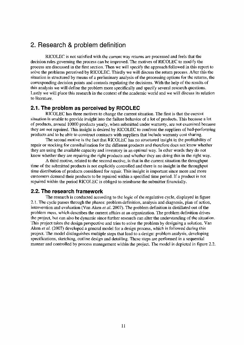
2.4.4. Decision points and rulesIn the return process multiple decisions need to be made with respect to the claim and the

submitted product. Figure 2.3 on the following page gives a claim and product flow diagramindicating the decision points, their order and structure. This diagram is only applicable to justifiedwarranty claims.

The model displays the flow of a claim and product through the process using an adaptationof the Petri-net modeling language (Jensen and Rozenberg, 1991). This language is highly appropriateto display the structure of processes. In the process depicted in the flow diagram three decision pointscan be discerned. The first is the decision whether to repair or not, this decision is taken for the claimand the product together. This decision is taken when the product is accepted as being covered underwarranty. If a product is not repaired, or when repair fails, the processing of the claim and the productneed to be done individually. Therefore, if this is the case, two more decisions need to be taken. Thefirst decision is how to settle the claim, either by replacing the failed product for a new one or byreimbursing the customer his money. The second decision deals with the product, should thesubmitted product be resold to a secondhand salesman or should it be cannibalized for useful spareparts. These two decisions are independent and always a consequence of the first decision and therepair process.

The decisions currently taken in the return process are governed by rules indicating whenwhich option is chosen. The decision rules in use are:

• Repair or not?: The decision is based on product type, ego a certain model of television. Ingeneral the products with the higher sales prices are repaired. However products that arereported as death on arrival (DOA), which means that they have never functioned and didnot function from the first attempt of use, are never repaired.

• Replace or reimburse?: Generally reimbursement is the used option. Only if the submitterhas specifically stated he wants a replacement product one is given. If a product is notcomplete when submitted (eg. a audio set is submitted without speakers) the submitted partof the product is replaced when possible. Else the claim is reimbursed upon receipt of theremaining parts of the product. If a repair fails the decision is taken based on the samecriteria.

• Stock or sell?: Products that are not repaired are sold. However DOA products of producttypes that are normally repaired are stocked for parts if the repairmen consider a largerinventory of spare parts necessary. Products that are repaired but the repair failed are alsoconsidered for cannibalization. In this case the decision whether more stock is necessary istaken by the repairman based on his opinion.

15

As can be seen, no rules are in place for the testing of products that are not considered for repair,therefore this decision is also not incorporated in figure 2.3.

y~s SUCCl!sfuJ· repair? yes

Fig. 2.3: Warranty return/product flow model

2.5. Detailed problem description & research questionsNow the possible courses of action for returned products and claimes are defined we can

specify the problem in more detail than the motives discussed in paragraph 2.1. Here we will firstformulate the problem in more detail and examine the costs and revenues associated with the differentcourses of action. We will conclude with the research questions coming forth out of the problem.

2.5. 1. Processing options: costs and benefitsThe challenge in this project is to redesign a set of decision rules that improve the

performance of the warranty return process, i.e. in terms of the realized reimbursement value ofrepaired products, on the one hand and to obtain more insights in the failure behavior of not repairedreturned products. In other words the decision what to do with a submitted claim and product shouldbe extended to include testing and improved.

The best warranty and product processing option for each product is determined by the costsand revenues associated with the first three possible options for processing of the product and the costand revenues of the options for settlement of the warranty claim for each claim. The costs of settling awarranty claim are either the costs of repair and redistribution of the product in case of repair, theprice of the replacement product and its distribution costs in case of replacement or the sales price ofthe original product in case of financial reimbursement. In case of unsuccessful repair the cost are thecosts of repair plus either the costs of replacement or reimbursement. The administration costsassociated with the processing of products are not considered, since they have to be made for allproducts and do not differ between products. Therefore it is assumed they do not influence the optimalcourse of action for a product.

The costs of the product processing options are based on multiple cost drivers. The costcomponents that can be discerned for each of the three product processing options are listed below.The costs of repair are determined by three components:

• The time needed by a repairman for repair of the product. This time is dependent on:o The type of product

16

o Type of erroro Product specific circumstances

• Costs of spare parts. These costs are dependent on:o The type of producto The type of erroro Supply situation (in stock/cannibalization)

• Overhead costs (building, equipment, etc.)The costs of cannibalization of a product are dependent on:

• The time needed by a repairman for cannibalization of the product. This time isdependent on:

o The type of producto Type of parto Product specific circumstances

• Costs of disposal of the remainder of the product. These costs depend on:o The type of product

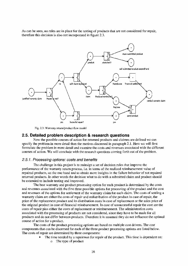
• Overhead costs (building, equipment, etc.)Only overhead costs are associated with the third option of the sale of the products to a foreign marketreseller. The revenues of this option consist of the price paid by the secondhand salesman.

The possible warranty settlement and product processing combinations and the associatedcosts and revenues are shown schematically in figure 2.4. The overhead costs are left out of thepicture, because they can be considered as sunk costs, since they cannot be influenced in this project.

Spare parts cost(cannibalizationl

new)

Transportationcosts (delivery)

Costs replacementproduct

Transportationcosts (delivery)

Costs:

Reimbursement fee

Costs:

Disposal costremainder

Costs:

No specificprocessing costs

Revenues:

Price paid bysecond hand broker

Fig. 2.4: Warranty settlement and product processing combinations cost structure

2.5.2. Research question(s)Taking the motives of RICOLEC and the preliminary analysis of the process, the decision

options and the associated costs into account we can formulate two main research questions for thisproject. The first is solely based on the first motive of RICOLEC since, as stated in the analysis, notesting of not repaired products is currently conducted.

How can RICOLEC obtain insight in the failure ofits products in the field by testing productsreceived in the warranty return flow?

17

The second research question incorporates the second and third motive of RICOLEC and addressesthe performance of the return process as described in paragraph 2.3. The question focuses on theallocation of products received under warranty over the different options open to the product and theclaim and aims to minimize the costs associated with processing the returns.

How should the submitted warranty claims and products flow be allocated to the differentsettlement/processing combinations in order to process the claims and products more cost-effectively?

To answer this question one has to take into account all the constraints that this process faces. If wetranslate this research question to the different decisions that need to be taken in the return process wecan formulate questions that can be addressed per needed decision.

To repair or not?:How to select the right amount ofproducts for repair?How to select the right type ofproducts for repair?

Subject to constraints with respect to throughput time and the fixed and limited capacity of therepairmen.

Replace or reimburse?:How to determine when a claim should be settled by replacement or reimbursement?

Cannibalize or sell?:How to select the right type ofproduct for cannibalization?How to select the right amount ofproducts for cannibalization?

Subject to constraints with respect to the fixed and limited capacity of the repairmen.

The questions, especially cannibalization and repair, are related due to the shared capacity ofrepairmen available for both actions.

2.6. Relationship to the academic literatureThe decision whether to repair or not needs to be made for every claim. In literature this is

termed order acceptance. In the models described in literature the accepting of an order hasconsequences. The order once accepted should be processed within the time allowed for itsprocessing. This is regulated by the scheduling function that determines when which order isprocessed. The order acceptance and scheduling function are therefore related and often discussedtogether in literature.

However, the situation observed at RICOLEC where a repair is useless once it is notperformed within the maximum throughput time causing a situation with immediate lost sales in caseof late delivery on the one hand, but on the other hand the decision whether or not to repair can alsobe changed after it is first taken, is different from the models discussed in literature as we will show inchapter 3.

Therefore, the situation discussed here, in which after an order is initially accepted it can stillbe decided not to repair the order after all and where costs associated with late repair equal the cost ofthe other processing options available to RICOLEC, namely reimbursement costs, is relevant to studyin view of the academic literature.

18

3. Literature study

From the problem definition a few areas of interest can be distilled. Here we will review therelevant literature on these areas in order to form a theoretical base upon which to focus in theanalysis of the current situation and more specifically in the design of a solution to the stated problem.

A number op topics is discussed. First we will shortly discuss warranties. After this a briefreview is given of the product failure related literature and the classification systems in the electronicsindustry. Thirdly warranty returns and their usefulness in improving product quality will be discussed.Fourthly we will discuss warranty return sampling. Fifthly we will focus on the repair department anddiscuss order acceptance, sequencing and throughput time regulation. The search method and termsused for this section can be found in Appendix 3. Sixthly, cannibalization and its uses andapplications are treated. Finally a conclusion is given.

3.1. WarrantiesWhen a justified warranty claim for a product is made by a customer a producer has the

obligation to equip the customer with a functioning product or reimburse the customer financially.The producer generally has, besides financial reimbursement, two possibilities to satisfy this request,he can either repair the send in product or redistribute a new product to the customer (Murthy et ai,2004). However it depends on the warranties in place how this process is arranged specifically.Important variables in the warranty are (Murthy and Blischke, 2005):

• Dimensionality of the warranty: A warranty is based on a number of variables. Normally timeis included, but use related variables like mileage can be included as well leading to amultidimensional warranty.

• Renewing or non-renewing warranty: If a warranty is renewing the warranty period ismeasured from the time of replacement. If a warranty is non-renewing it is measured from thetime of first purchase

• Free replacement I Pro-rata I rebate warranty: A free replacement warranty supplies thecustomer with a replacement for free, while a pro-rata or rebate warranty obliges the supplierto supply either a (partial) monetary refund (rebate) or a replacement at discounted costs (pro­rata) to the customer.

With these variables numerous combinations can be made, leading to the many different types ofwarranty that exist. The options are further extended by options like exemption clauses, that exemptcertain parts (partially) from warranty, and cumulative warranties that cover groups of items (Murthyand Blischke, 2005).

Another variable, not explicitly warranty related, although it might be defined in the warranty,is the type of product distributed to the customer. If a replacement is given, this can be a new productor a repaired product. A new product has a failure distribution similar to a new bought product. This isnot certain for a repaired product. In literature two types of repair can be distinguished, both at oneend of a spectrum. On the one end is repair leading to an as good as new product. On the other end isrepair leading to a product just as good as the failed one, except without the failure. These productsdiffer with respect to their failure rate. The first has the failure rate distribution of a new product, thesecond the distribution of a product already used for some time. The decision whether to replace orrepair therefore is dependent on the quality of repair. For heuristics and optimal proceduresdetermining time intervals for repair and replacement see Jack and Van der Duyn Schouten (2000),Jack and Murthy (2001) or Murthy (1996).

Besides the legal obligations present to satisfy justified warranty claims, a number of reasonscan be present for a company to take back the products or parts of products on which the warranty isclaimed. Flapper (2005) distinguishes ten reasons which vary from the prevention of fraud to thefiling of claims at the company's suppliers.

19

3.2. Product failure & failure classification

3.2. 1. Product failureEvery product can break down. The possibility of breakdown however is different for

different products. In general, the variables determining the chance of failure include the quality of theproduct influenced by product specifications and production statistics, the time a product is in use andthe way a user uses the product (Brombacher et at, 2(05). However in the field the only easilyobservable characteristic is the time a product is in use. Neither the desires of the customer nor thestatistical variation in a product due to production are readily available. Therefore we will focus onthe failure behavior of products with respect to its lifetime.The chance a product fails at a specific point in time is defined as the failure rate. Traditionallyproducts were stated to have a high chance on failure early in their life followed by a low chanceduring their normal life and an increasing chance when old age was reached. The first high is causedby so called infant mortality, the second high chance by fatigue and wear-out. This results in thewidely used bathtub curve shape indicating the chance a product fails, see ego (Wang et at, 2002).

With regard to electronics research showed that several branches of electronics industryfollow a curve known as the roller coaster curve (Lu et at, 2000). This curve is displayed in Figure3.1.

random failures

hnmedlate failure

delayed observation I reporting

t

Sub-population, rapid wear-out I

increased 0 r increasing sttess

Systematic lNear"out IIncreasing stress

Time ..Fig 3.1 The roller coaster curve (Lu et aI, 2000): Failure rate over time

Compared to the bathtub curve one phase is added, phase 2. This phase is caused by the combinationof users that use the product extremely intensive, more intensive than anticipated, and weak productsas a result of variation in production. This combination leads to rapid wear-out, however this onlyhappens in a subpopulation of the total group (Lu et at, 2000). These failures are important forwarranty, since they often occur within the warranty period.

3.3. Warranty returns, product quality & failure

3.3. 1. Field feedback & product qualityProduct quality is determined by a variety of factors. Next to product design, user

expectations and material quality among others playa role. For manufacturers to improve on theirquality levels the weaknesses in current product user combinations need to be known. Differentsources are available in the field for this information (Petkova, 2003). One of these sources iscomprised of the failed products send return.

Petkova (2003) distinguishes two types of information, engineering information and statisticalinformation. The former includes the information necessary to find the cause of a problem, thus is

20

vital for product quality improvement. The latter includes the frequency of returns and furtherstatistical information involving product returns. This information is useless for product qualityimprovement without engineering information, however in combination with engineering informationit gives a detailed image of the quality of a population of products and can greatly help to identify themost profitable quality improvements.

Petkova (2003) concludes that field feedback is usually too late to facilitate qualityimprovement of products and that it is hardly possible to improve this because of the time delaysinherent in the matter. Nonetheless engineering information can be of use in the design of subsequentproduct types, especially if standard designs are used as is the case in the mass-production consumerelectronics industry (Petkova, 2003).

An example of a classification method for engineering information is the IRIS code used bythe majority of service centers in the brown and white goods. Petkova (2003) states that the IRIS codeinformation is not useful to find the underlying cause of a reliability problem. This because it is notdetailed enough, because it only describes the symptom and its diagnosis, and because the interactionbetween the product and its surroundings is not considered. Lastly she states that the indicatedlocation of the failure has not necessarily caused the problem. Nonetheless the system has itsadvantages in its ease of use and its wide applicability and usage. Besides, the system does assist infinding the final failure mechanism on a part or module level which can serve as a starting point forfurther examination by the manufacturer. Also the argument of not considering the interactionbetween the product and its surroundings becomes irrelevant when multiple products are examinedper product type since probabilities that failure comes from extreme usage for all returns is very smalland can be defined as bad product design. Therefore we will give an explanation of its origin, basisand functioning.

3.3.2. The IRIS classificationIn the mid '80s SONY was the first electronics manufacturer that made factories responsible

for the quality of their products and therefore also must bear the warranty costs of those repairs. Thisresulted in a need for information on the performance of products on the market. This need wasfulfilled by after-sale service organizations. However the communication between service/repairorganizations and the producers was faced by difficulties like geographical differences, language andthe fact that most repair was done by external companies (authorised servicers and dealers). Thereforea standardized Repair Description Language was developed by SONY (IRIS30urse, presentation ofEICTA).

This language now serves as the basis for the International Repair Information System,abbreviated IRIS. This language is used in Europe and Japan for the coding of failures and repairs ofbrown goods. An effect of the standardization is the codes presence in most repair administrationsoftware (IRIS_course, presentation of EICTA).

The IRIS code consists of 6 different parts and codes the symptoms, diagnosis, defect andrepair. Next to that it indicates the type and number of spare parts used during the repair. An exampleof an IRIS coding strip is shown in figure 3.2, with this figure we will explain the different parts ofthe code.

21

Part Pas -NoPart-No

_•.••111

•Fig. 3.2: An IRIS classification strip (How Iris Works, presentation of the EIeTA)

The parts are represented by the different colors used in the figure (IRIS_course, presentation ofEICTA) :

• Condition code: This part is filled in by the customer and describes the conditions underwhich the failure takes place. When it is hot or humid. Conditions should be noticeable by a"ordinary" customer

• Extended condition code: The condition code can be extended to include at which part of themachine and during which functional performance the defect is observed. For instancewatching DVD's the lower left comer does not work. This is done by a customer

• Symptom code: Here the symptoms of the defect are described by the customer. For instanceno sound, or no vision. In some countries two symptom codes are entered, next to thecustomer, a technician also describes the symptoms here

• Part number, quantity and position: This is manufacturer dependent and gives the preciselocation, number and type of parts malfunctioning and repaired/replaced. Sometimes even theplace on the part (for module structures, or printed circuit boards for instance) can beindicated

• Defect code: Here the technician specifies the defect he has found. This can relate to themalfunctioning part. However the defect can also be of a software nature or no defect can befound at all

• Repair code: The technician indicates what he has done to fix the defect. If the defect wasfixed he adds a flag. It can be that he performs multiple repairs for one defect, then the onethat fixed the problem is flagged. Also repair codes like software upgrading or return withoutrepair are possible here.

All input on the sheet is coded to prevent language problems. For every type of machine codes existthat correspond with the type of condition, symptoms, defects and repair possibilities. The tables withthese codes and corresponding meaning are available in all European languages; an example of a tableused at RICOLEC is displayed in Appendix 3.2.

The advantages of IRIS accrue to all parties involved. The servicer/repair company canhandle their repairs more professionally, accurately and faster because of the structured data input.The manufacturer gets structured, insightful data on problems and therefore can address theseproblems more easily in new generations of products (IRIS_course presentation of EICTA).

3.4. IRIS-cIassification warranty samplingSince testing all products is very time consuming, we will shortly address the option of

sampling to obtain information on the failure of products. IRIS-codes only classify a failure. They donot give a hierarchy. Therefore one cannot speak of a mean IRIS-code. However, some failures occurmore frequently than others, and this information is of interest in countering failures, as expressed in

22

the previous section. A way to obtain infonnation on the frequencies of occurrence is by sampling andregistering the obtained IRIS-codes.

The sampling of nominal data is based on the representativeness of elements in a populationfor that population. A good sample is accurate, which means unbiased, and precise, which means thatthe error in the sample is sufficiently large to draw conclusions. Since a sample relies on part of thepopulation it is never completely sure the resulting estimate is the true value, the precision determinesthe interval for the estimate and the degree of confidence one can have that the real value is in theinterval (Cooper and Schindler, 2003).

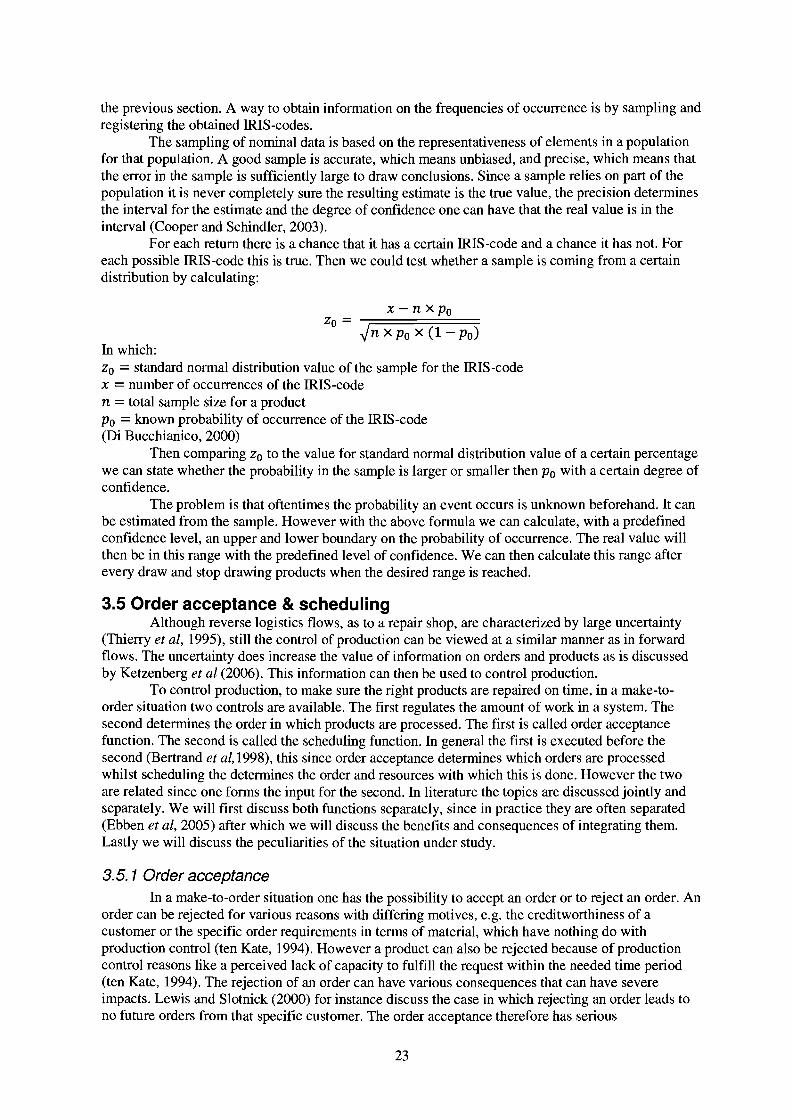
For each return there is a chance that it has a certain IRIS-code and a chance it has not. Foreach possible IRIS-code this is true. Then we could test whether a sample is coming from a certaindistribution by calculating:

x - n x PoZo = --;::::.===:::=:==::::::::.In x Po x (1 - Po)

In which:Zo = standard nonnal distribution value of the sample for the IRIS-codex = number of occurrences of the IRIS-coden = total sample size for a productPo = known probability of occurrence of the IRIS-code(Di Bucchianico, 2000)

Then comparing Zo to the value for standard normal distribution value of a certain percentagewe can state whether the probability in the sample is larger or smaller then Po with a certain degree ofconfidence.

The problem is that oftentimes the probability an event occurs is unknown beforehand. It canbe estimated from the sample. However with the above fonnula we can calculate, with a predefinedconfidence level, an upper and lower boundary on the probability of occurrence. The real value willthen be in this range with the predefined level of confidence. We can then calculate this range afterevery draw and stop drawing products when the desired range is reached.

3.5 Order acceptance & schedulingAlthough reverse logistics flows, as to a repair shop, are characterized by large uncertainty

(Thierry et ai, 1995), still the control of production can be viewed at a similar manner as in forwardflows. The uncertainty does increase the value of infonnation on orders and products as is discussedby Ketzenberg et ai (2006). This infonnation can then be used to control production.

To control production, to make sure the right products are repaired on time, in a make-to­order situation two controls are available. The first regulates the amount of work in a system. Thesecond determines the order in which products are processed. The first is called order acceptancefunction. The second is called the scheduling function. In general the first is executed before thesecond (Bertrand et ai, 1998), this since order acceptance determines which orders are processedwhilst scheduling the detennines the order and resources with which this is done. However the twoare related since one fonns the input for the second. In literature the topics are discussed jointly andseparately. We will first discuss both functions separately, since in practice they are often separated(Ebben et ai, 2005) after which we will discuss the benefits and consequences of integrating them.Lastly we will discuss the peculiarities of the situation under study.

3.5.1 Order acceptanceIn a make-to-order situation one has the possibility to accept an order or to reject an order. An

order can be rejected for various reasons with differing motives, e.g. the creditworthiness of acustomer or the specific order requirements in terms of material, which have nothing do withproduction control (ten Kate, 1994). However a product can also be rejected because of productioncontrol reasons like a perceived lack of capacity to fulfill the request within the needed time period(ten Kate, 1994). The rejection of an order can have various consequences that can have severeimpacts. Lewis and Slotnick (2000) for instance discuss the case in which rejecting an order leads tono future orders from that specific customer. The order acceptance therefore has serious

23

consequences. Accepting too many orders leads to overload and an increasing number of late products(Ebben et at, 2005), whilst accepting too few orders leads to low utilization rates and less profit.

In our scenario the costs related to the rejection of an order are equal to the costs of latecompletion of an order, no extra costs are incurred. We do have limited capacity and too many orders.Therefore the production control motive to reject orders is apparent. We should then decide whatshould form the basis for the decision to accept or reject an order. Either the profitability of the ordersor the available capacity can be leading in this decision.

Two general ways can be discerned to control the flow of work through a production process.The first is based on demand, which consist of orders, and in its purest form pushes work into theprocess without looking at the status of the process. Therefore production systems under this type ofcontrol rules are called push systems. The second way is based on the available capacity in thesystem. Orders are accepted if capacity is available. These rules pull work into the system if capacityis free, hence the name pull systems (Hopp and Spearman, 2000).Research has indicated that in situations where both push and pull systems can be applied pullsystems are favorable. This because pull systems have a lower Work In Process (WIP) for the samelevel of throughput and therefore lower cycle and throughput times for the same throughput rates.Also a pull system is more robust to errors in WIP than push systems are for errors in release rate(Hopp and Spearman, 2000). In practice of course hybrid systems using both push and pullmechanisms exist and the distinction is not this sharp. For a discussion on the merits andshortcomings of both push and pull systems we refer to Zijm (2000).

The focus should then be on capacity oriented order acceptance. Kingsman (2000) describesinput and output control for one machine, first come first served processing and fixed due dates. Ifthe queue plus the input exceed a certain value the due dates can be exceeded, this relation holdsregardless of the control method used. This can be prevented by reducing input by rejecting orders,input control, or increasing capacity, output control (Kingsman, 2000). This method of throughputtime regulation through input control can also be found in a specific Pull system called CONWIPcontrol (Hopp and Spearman, 2000). In this system WIP is controlled by specifying a upper boundaryon the WIP in the system. If this boundary is reached no new products are admitted into the system.This ensures no WIP explosion and thereby controls throughput times. The problem of setting thelimit on WIP, known as the WIPcap, and controlling the WIP is referred to in literature as card settingand controlling (Framinan et at, 2003). Card setting refers to the setting of a WIPcap level based oncertain operating measures whilst card controlling refers to the updating of the WIPcap level based onchanges in certain variables such as demand, processing times or capacity. Card setting is widelydiscussed in literature, but no clear rules have been formulated and the decision generally involves atrade off between desired service level, the percentage of products delivered on time, and the WIPlevel (Framinan et at, 2003). A method used is based on Little's law where the desired throughput andcycle time lead to a WIPcap level (Huang et at. 1998). Card controlling is not widely discussed inliterature. An extensive review of the literature card controlling and the (dis)advantages of controllingover card setting can be found in Framinan et at (2006).

The CONWIP approach, regulating WIP below a certain level which is never exceeded, hasshown to perform well in various situations all involving equal products (e.g. Roderick et at, 1993).However, its performance when multiple products of different importance need to be processed is, toour knowledge, never examined. In this situation the rejection of some orders is more severe than forothers; however the CONWIP system does not discriminate between these orders and thus lesslucrative orders can be processed instead of lucrative ones (Van Ooijen and Bertrand, 2003). It isexpected that the more often the WIPcap is reached the more severe this problem becomes.

3.5.2 SchedulingAfter acceptance, accepted orders should be scheduled to make sure the products are

processed in an order that maximizes the profit obtained. In literature numerous different schedulingalgorithms can be found with different focuses. Some minimize the total lateness, which is thedeviation from the Due Date either early or late, of orders, whilst others focus on the minimization oftardiness (e.g. (Abdul Razaq et aI, 1990) (Yang et aI, 2004)). In our situation, the number and value of

24

the tardy jobs is the relevant criterion. Therefore we will discuss its minimization in a little moredetail.

3.5.2.1 Minimization of the number of tardy jobs

A job is tardy when it is finished after its Due-Date. For some jobs this is worse then for otherjobs, since jobs can have different importance. Therefore the tardiness of jobs needs to be weightedwhen it is minimized. The minimization of the number of tardy jobs on one machine, when all releasedates are equal and processing times are deterministic and known can be achieved with the algorithmof Hodgson (Moore, 1968) which is computed as follows:

1. Rank all products on Due-Date, starting with the earliest2. If no or just one order is late this is the optimal sequence. If not determine the first late order

in the sequence3. Now find the order with the largest processing time in front of the first late order and place it

at the back of the queue.4. Repeat step 2 without considering orders that were placed in the back of the queue.

Lawler (1994) shows this algorithm can be applied when processing times and weights areagreeable, meaning smaller products with smaller processing times have larger weights. Also branch­and-bound methods have been developed for the situation where all products are released on the sameday (Potts and Wassenhove, 1988) as well as Lagragean relaxation based heuristics for the situationwith equal weight but different release and due dates (Dauzere-Peres, 1995).

Heuristics for non-agreeable varying weights and different release and due-dates, the moregeneral case, have been developed using Lagragean relaxation (Sevaux and Dauzere-Peres, 2003)(M'Hallah and Bulfin, 2007) and Genetic Algorithms (Sevaux and Dauzere-Peres, 2003). Howeverthe obtained results for upper and lower bounds, especially when the number of jobs is larger then100, lead the authors to conclude that the heuristics performance is not guaranteed to be high,especially for weighted cases. Besides this the computational time to solve the heuristics and exactsolutions is large, with all discussed heuristics, except M'Hallah and Bulfin's heuristic, requiringmore than one hour computing time in numerous cases (M'Hallah and Bulfin, 2007).

A requirement for the implementations discussed above is that products are individuallyaccessible for sequencing and that processing times are deterministic. In case of non-deterministicprocessing times the solution can still be used, however their performance in terms of optimalitymight be influenced. If products are stocked in batches none of the discussed algorithms andheuristics can be implemented as such and the situation is severely complicated when the batches donot consist of products of the same importance.

We can however sequence batches on other characteristics which are equal to all products inthe batch. In our case this is the entry date and the maximum throughput time of the products in abatch, thus the Due Date of the products in the batch.

3.5.2.2 Due-Date Scheduling

Due Date (DD) scheduling entails that products that need to be finished on an earlier datehave priority over products with a later due date and are processed earlier (Bertrand et al, 1988). In acase in which all products have equal desired throughput times no difference exists between DD andFCFS scheduling. However if some products have other desired throughput times than others DDscheduling will lead to very different results than FCFS. The performance of the DD rule compared tothe FCFS rule is highly dependent on the variation in desired throughput times. The DD rule, andother delivery oriented rules, primarily influences the spread of the throughput time attained. They donot influence the mean throughput time. Bertrand et al (1998) show that the spread in throughput timefor the DD rule is nearly halve the spread of the FCFS rule at given production circumstances.

3.5.3. Joint order acceptance and schedulingSince the two control mechanisms are interrelated it might be wise to take scheduling into

account when deciding on order acceptance. However this complicates the decision. Ebben et al(2005) make the distinction between order acceptance policies and order acceptance algorithms. A

25

policy does not require computations upon the entering of each new product, the decision is based onthe state of the system as in the order acceptance literature discussed above. An algorithm does needcalculations, for instance to calculate a schedule that incorporates the newly accepted product, whichmay require extensive computing time. In a policy the order acceptance and scheduling are largelyuncoupled, whilst in an algorithm they can be closely interrelated.

Ten Kate (1994) examined the influence of integrating the two in an algorithm compared tothe hierarchical approach in which order acceptance is performed first and found that in general thereis little difference between the two. Only with short lead times and high utilization the integratedapproach outperforms the hierarchical approach. Wester et al (1992) arrive at a similar conclusion, intheir evaluation of an integrated algorithm and two hierarchical policies. Only if set-up times are largeand due-dates are strict the algorithm outperforms the policies.

Nonetheless several contributions have been made to the integration of the two functions, seee.g. Rom and Slotnick (2008) for an overview. However most ofthese contributions assume knownarrivals and deterministic processing times. Besides the dominant optimization criterion is tardinessand not the number of tardy products.

3.5.4. Order acceptance, scheduling: peculiarities of the situation under studyAll the discussed literature assumes that when an order is accepted, it also needs to be

processed. The possibility of alternative options to fulfill the order and in this way regulate productionis not taken into account, probably because this option is not considered feasible. In situation understudy this however is feasible. After an order is accepted, it can still be decided not to repair theproduct after all.

Depending on the way this order is then processed, still by repairmen or by other employees,we could say we can either influence processing time at higher processing costs or outsource theorder. Both these options are discussed for related situations in literature.

Lee and Sung (2008) discuss the scheduling problem with outsourcing allowed. They assumea fixed cost per order for outsourcing and a maximal budget for outsourcing and then develop twoheuristics to minimize the maximum lateness and total tardiness. In the heuristics they first determinethe set of jobs that needs to be outsourced after which they sequence the other jobs. If products arestored in batches however the proposed heuristics become infeasible since products can then not beoutsourced individually.

Chen et al (1997) discuss the discrete regulation of processing times. They conclude that ifthe goal is to minimize the number of tardy jobs the problem is NP-hard in line with the schedulingliterature discussed above. However they do state an optimal solution exists and give a fewcharacteristics that the optimal sequence needs to satisfy.

Concluding, looking at the model described by Kingsman (2000) in this project besides theinput level also the amount of work in the queue can be regulated by not repairing products if toomany products are in the queue at the repair department. If all products would be equal this optionwould not add anything to the order acceptance function, however if products are not equallyprofitable this permits the preference of more rewarding orders over less rewarding orders when achoice needs to be made in view of the possible late repair of orders.

3.6. Cannibalization & inventory management of spare partsCannibalization is defined by Thierry et al. (1995) as the recovery of a limited set of reusable

parts from products or components. Cannibalization involves the selective disassembly of products tofind the reusable parts. The remainder of the product can be processed in different ways.

Cannibalization can be used as a method to obtain spare parts needed for the repair of failedproducts (Thierry et al. 1995). The spare part inventory management system however will beincreasingly complicated by the addition of cannibalization. An overview of the literature on sparepart management in general can be found in Kennedy et al (2002). Spare part management systemsinvolving cannibalization are not discussed in literature. However models involving cannibalization ina remanufacturing situation are discussed, e.g. Van der Laan et al (1996).

Vander Laan et al (1996) discuss the extension of normal stockkeeping policies with optionsto obtain parts from cannibalization and disposal opportunities for these parts. For the extended

26

policies exact expressions for the costs are derived. From the paper it becomes evident that policiesusing cannibalization as well as the new purchase of parts are more complex that single sourceinventory systems. If one adds the increased complexity of spare parts inventory management system,it is easy to imagine the complexity of a spare parts inventory management system sourced bycannibalization and new part purchase. The amount of information necessary to develop and maintainsuch a system is very large and includes the demand for spare parts, the arrival pattern of returns andinformation on the quality of returns among others.

3.7. ConclusionThe relation of this project to the academic world will be in the field of production control of

a make-to-order company. We will focus on the order acceptance function and discuss the differencesbetween the situation in which all products that are accepted need to be processed in the same mannerand the situation in which the processing can be regulated on two levels, with zero profit for the fastlevel, based on the amount of orders accepted. Both systems are regulated by a Work in Process(WIP) based order acceptance policy. Besides this we will examine the performance of a CONWIPlike production control system for variable profitability products. Lastly we will discuss the possibleimprovements attainable by individual stock keeping of orders instead of in batches as forms the basefor the systems discussed above.

27

4. Detailed analysis of the current situation

Under the current decision rules the different settlement/processing combinations defined anddiscussed in Chapter 2 are used to a different extent. The repairmen as a consequence are performingcertain types of repairs on certain types of products and some parts are purchased whilst others areobtained through cannibalization.

First we will examine the magnitude and composition of the warranty return stream and wewill examine the time interval between purchase by the user and the filing of the warrantee claim.

Secondly we will look at how the flow is divided over the different claim settlement optionsand analyze the decision rules used to obtain this division. Here also the processing of Death onArrival (DOA) failures is discussed.

Thirdly we will zoom in on the repair department, for which we will examine what tasks therepair department is performing and examine its total capacity. After this we will further analyze thetasks performed and the average time needed to perform them. Also the throughput times of the repairdepartment will be analyzed.

Fourthly we will examine the failure behavior of the different product groups. An analysiswill be made of the occurring failures and the corresponding repair actions.

Fifthly we will shortly discuss the inventory management of spare parts before we give asynthesis indicating the opportunities for improvement of the present situation.

For the analysis the figures on the returns received in 2006 will be used. These figures,according to RICOLEC, give an accurate representation on the division of products over the differentprocessing options, although the importance of the different groups has changed since 2006. Themagnitude of the return flow in 2005 to 2007 is also known, in the discussion on the magnitude of thewarranty return flow these figures are used in the analysis.

4.1. Magnitude and composition of the warranty return flowRICOLEC has received between 18000 and 25000 warranty returns yearly for the last 3 years.

There is no clear increasing or decreasing trend in the number of warranty returns. These returns aredistributed evenly over the year, although some seasonality can be discerned from 2005 onwards.Peaks in the returns are observed from January to March and in August. The number of returns eachmonth for 2005 to 2007 and the average seasonality factors for the different months are displayed inAppendix 4.1.1. This factor was determined by dividing the number of returns received in each 4week period by that year's average for 4 weeks leading to a normalized index.

The distribution of returns in a week is not uniform. Tuesdays and Thursdays each accountfor about 25% of the returns whilst the other 3 days account for equal percentages of about 17%. Thisis because two large logistic service suppliers deliver returns twice weekly, on Tuesdays andThursdays. When both effects, the seasonal and the day effect, are deleted from the returns bydividing the received returns by the multiple of both effects, the return flow in 2005 to 2007 can beassumed to be normal distributed with a varying mean for the years but a similar standard deviation,as is shown in Appendix 4.1.2. The distribution characteristics, especially the P-value scores, indicatethat the returns can be assumed to come from a normal distribution.

RICOLEC is responsible for and receives the returns from the Benelux. RICOLEC normallyoffers one year warranty on their products, although CEB products are offered with two yearswarranty and CED products with three years.

The product portfolio of RICOLEC is large. It covers multiple brands and different productgroups (e.g. home cinema, LCD television etc). Next to that products are renewed quite fast in theconsumer electronics branch, whilst warrantees generally cover a longer period. This combinationleads to a very diverse product type composition of the warranty return flow. In 2006 for instanceover 300 different product types were submitted within warranty, at the moment this number isestimated to be around 200.

Within RICOLEC product types are classified within groups based on their functionality andthe used techniques, e.g. LCD-televisions and CRT-televisions are two different groups. RICOLECdistinguishes 17 product groups. Table 4.1. lists these product groups with a description of their

28

functionality and the used techniques. The table also lists VCR players. However VCR players are notsold anymore and are also not covered under warranty anymore, but are still repaired on customerdemand because of customer service considerations. Some product groups are being phased out (KTVand MP3 players) whilst others (LCDtv and LCDIDVD combo) are getting increasingly important.All product groups consist of multiple product types. The percentage of the total sold products whichis returned under warranty, the warranty return rate (WRR), varies between product groups but evenmore between product types as can be seen in appendix 4.1.3. Within one group WRRs of 1 to 15percent are observed, the failure behavior, in numbers, is thus strongly product type specific. Thedifferent product groups have different average WRRs, and RICOLEC uses different percentages ofWRR to judge the performance of products. The percentages are based on the estimated quality of theproduct. The division of the returns over the different product groups is depicted in Appendix 4.1.4.

Product aroup DescriptionHome cinema Home cinema systems with DVD and surround sound equipment

KTV CRT color televisions

LCD LC0 color televisions

Combo Icd/DVD LCD color televisions with an integrated DVD playerCombo

TV/video/DVD CRT color televisions with an inteQrated DVD or VCR player

Port.DVD Portable DVD-players with a small LCD screen

DVD-player ReQular DVD players without sound functionality

Video VCR players (not for sale anymore)

Audio set ReQular Audio sets with a tuner and CD player

Port. radio/cd Portable audio sets with a tuner and CD player

Discman Portable CD players with headphones

Alarm clock Alarm clock indicating time and with radio functionality

Radio Normal Radios

Car stereo Car stereo systems with radio and CD player

Telephone DECT-telephones

PMR Personal messaging radios (walkie-talkies)

MP3 player Portable MP3 players

Other devices like speaker standards, earphones and other small devicesTable 4.1: Product groups for warranty returns at RICOLEC

The overall average time between customer purchase and the filing of the warrantee claim is160 days, which is about six months. However we need to split this figure according to the warrantyperiod given to the customer. In Appendix 4.1.5 a histogram in which the period between customerpurchase and warrantee is depicted for products with one year warrantee (N=5939 products). Theseclaims are averagely filed after 156 days which is about 5 months and only a very small decline inclaims can be found during the warranty period. Appendix 4.1.5. displays a histogram for productswith two years of warrantee (N=95 1 products). Here we see a clear decreasing pattern over thewarranty period. These returns can be modeled by an exponential distribution with a mean of 158days. For products with 3 years of warranty only limited numbers, 30 products, have been sold andsales only commenced in 2006. Therefore the relationship between purchase and warranty can not beanalyzed representatively at the moment. It is surprising that the average time between purchase andclaim filing is nearly equal for one and two year warranty periods offered. This implicates thatoffering larger warranty periods does not lead to equally larger costs associated with warrantees.

29

4.2. Division over the settlement/processing options

4.2. 1. OverviewThe return stream can be divided into warranty and non-warranty returns. For the warranty

returns three claim settlement options are available to RICOLEC, namely repair, replace andreimburse. For the non-warranty returns either a repair or replace proposal is made or nothing is doneat all. We will look at the distribution of the total number of returns over these options. Also theproduct group mix is examined for all the options. Lastly a conclusion will be drawn on the allocationrules used to determine what settlement option should be used.

4.2.2. Repairs not related to claimsOf all the returns received in 2006 only 5% was not covered under warranty. This percentage

fluctuated from 4,0% to 6,3% monthly. The product mix of these returns can be found in Appendix4.2.1 86,7% of the products were sent to the repair department for inspection and a repair/replaceproposal.

It is unclear whether a proposal either for repair or for replacement is made to the submitter,since this cannot be seen out of the IRIScodes. However out of the registered IRIScodes it can beconcluded that of all the inspected products 50,5% is repaired, 12,0% is replaced and in 33,7% of thecases the proposal is declined. Finally 3,3% of the products is sent back without repair because thesubmitter fails to accept or decline the proposal.

4.2.3. Warranty returnsThe division of the returns under warranty over the product groups can be found in Appendix

4.2.2 Of the 21000 returns received in 2006 95% was covered in warranty.

4.2.3.1. Repairs

Of the warranty covered products 35 to 40% were sent to the repair department for repair, thisfigure can not be determined exactly because of inconsistencies, e.g. typing errors, or a lack of clarityamong repairmen on the meaning of the codes, in the repair administration process. The bothestimates are based on different definitions of what constitutes a repair, with the higher estimateincluding dubious entries that could have been the results from the inconsistencies. Variationsbetween months, when using the 40% estimate, were between 36% and 48%. Figure 4.3 displays thedivision in product groups of the warrantee covered repairs.

30

• portable LCD-DVD player

• audio-setIII home-cinema

• KTV DVDlvideo combiDKTV

• DVD-player• MP3-playero portable Radio-CD player

• LCD-tv.VCR.discman

• LCD-tv DVDlvideo combi

• telephoneo radio

• unknown• alarmclock• other

Fig. 4.3. The division of the repaired warrantee returns in product groups

4.2.3.2. Product replacement and reimbursement

60 to 65% of the warrantee returns were not repaired. Of these claims 75% was settled byfinancial reimbursement and approximately 15% was settled by replacement of the product, thesettlement options chosen for the other 10% is unclear. The division over the product groups can befound in Appendix 4.2.3

4.2.4. Allocation rulesThe allocation rule used to identify whether a product is a warranty return or not is

straightforward. It depends on whether the warrantee period has expired and whether the product wasused in a normal manner by the customer, although this is very hard to verify. The allocation rulesthat determine how to process warranty claims on the other hand are not so straightforward. Here wemake the distinction between repair and the other two options. The allocation rules used to determinewhether a product should be replaced or reimbursed could not be explicitly derived from the availableinformation on the processing of products. In practice this decision is taken based on specificcustomer preferences and/or the inventory situation of new products for the specific product typesince a product must be available in order to be able to replace it. Often it is difficult to replace aproduct because only newer versions of the product are available. These versions are seldom acceptedby the submitting companies. This leaves only the option of financial reimbursement open to satisfythe warranty claim.

The decision whether to repair a product at a first glance seems to be taken on a productgroup level. Some product groups are considered for repair more often than others. The productgroups most often sent to the repair are Home cinema (92,5% of the arrivals), LCD (92,1 %) andportable DVD (91,1 %). Other product groups often sent to the repair department include KTV,Combo TV/videoIDVD, audio-sets, VCR, DVD-player and combo LCDIDVD. For the other productgroups repair is undertaken on less than 30% of the returns. The full results per product group can befound in Appendix 4.2.4. A closer look reveals that the decision whether to repair a product or notseems to be taken on product type level. In the KTV and audio-sets categories for example, some

31

product types are repaired very frequently whilst other types are not repaired at all. The results foreach product groups' product types can be found in Appendix 4.2.4

Because of the existence of Death on Arrivals (DOA), which are never sent to the repairdepartment, the percentages sent to the repair department of most product types generally consideredfor repair do not equal 100%. As noted in the second chapter, the processing of products classified asDOA is different from 'normal' return processing. These are not repaired, even though other failuresof the same product type are repaired. Also the processing options for DOA' s are more diverse. Theycan be cannibalized, sold secondhand or repaired with the intention of making a new sale. This lastoption, according to the repairmen, is currently never used. The quantity and manner of processing ofDOAs cannot be analyzed from the available figures.

4.3. Capacity, tasks & performanceThe tasks in the return processing are performed by two departments. The arrival and the

handling of not-repaired (warranty)returns is undertaken by the collection department. The repair ofproducts, whether under warranty or not, is done by the repair department. This department alsocannibalizes products to obtain spare parts. Here we will first shortly examine the tasks andperformance, in terms of throughput time, of the collection department. After this we will examine thecapacity, tasks and performance of the repair department.

4.3.1. The collection departmentThe collection department is generally staffed by one person except on Tuesdays and

Thursdays, when two persons are employed. This because more returns arrive on these days. At thecollection department ample capacity is present to register all claims arriving on a day the same day.The take in process was already sufficiently described in section 1.2.1. of this report.

The further processing consists mostly of administrative tasks, the exception being when areplacement product needs to be taken from stock, wrapped and made ready for transport. The preciseprocess and its parts is not part of our research and therefore will not further be examined. Howeverwe will take a short look at the throughput times of the products completely handled by the collectiondepartment, to examine whether these products are processed within the maximum throughput timesstated by RICOLEC's customers. The throughput time for these claims is small. In general theseclaims are processed immediately or shortly after arrival. This because it is an administrative, not timeconsuming, task consisting of booking the product in and ensuring financial reimbursement for thesubmitter. However it can be that because of incomplete products send in with the claim or otherdifficulties this time is severely lengthened. Overall 50% of the claims is handled by the collectiondepartment within 4 days and 91 % is handled within 14 days, thus within 10 working days. The delayis mostly caused by the incorrect filing of customers.

4.3.2. The repair departmentThe repair department does not have ample capacity to repair all (warranty)products. Besides

this the department has some other tasks to perform as well. Here we will first look at the tasksexecuted by the repair department. Then the available capacity and its division over the tasks areexamined. Lastly we will look at the performance of the repair department in terms of throughputtime.

4.3.2.2. The tasks

The tasks performed by the repair department are:1. The repair of products under warranty2. The inspection and repair of products out of warranty3. The cannibalization of products to obtain spare parts

We will briefly explain the steps and their durations in each of these tasks.

4.3.2.3. Repair under warranty

As described in the first chapter the repair of products under warrantee consists of severalsteps. These steps are: getting the product from the container, unwrapping the product, look up the

32

product in the database, inspect and repair the product, wrap the product, finish product administrationand put the product back in the container. In this process the inspection and repair step is dominantfrom a time perspective. The time needed for the other steps is very limited. All the other stepstogether take an average of 3 to 4 minutes. This time is fairly constant.

The repair and inspection step can be further subdivided. First a product is connected, then thecomplaint is checked. Depending on the complaint and whether it is detected further actions are taken.Most of the times an attempt at repair is made. This attempt involves opening the product, repairing orreplacing the broken parts and closing the product again. After this it is checked whether the defect issolved. The connecting and checking of the complaint takes about I to 3 minutes and the checkwhether the defect is solved takes I to 5 minutes. Products for which the complaint is not found arenot opened, but their functions or specifications are tested. The time needed to open and close theproduct is highly variable among product types and constitutes a major part of the total repair time.The time needed for the repair of the defect is highly variable among product groups and dependenton the size of the products. In larger products (LCDtv, DVD-players etc.) it is easier to find thefailing components than in small products (Portable LCD-DVD players) where all the components arefitted in very closely and it is often necessary to remove working parts to get to the failing parts whichis very time consuming. If an attempt is taking about 30 minutes and still no end is in sight the attemptis ended and the claim is settled by different means. The product is either stocked for cannibalization(50%) or sold secondhand (50%). Only very rarely a product is disposed of. All in all it is estimatedthat 30 minutes per product is a very rough but useful estimate. The specific time needed to solve aspecific repair on a specific product will be examined in section 4.4.

4.3.2.4. Repair out of warranty

When a product out of warranty arrives at the repair department first a proposal needs to bemade for repair or replacement of the product. During the inspection to make the repair or replaceproposal the section of failure and the defect are classified, the time needed for this is estimated by therepairmen to be only 2 or 3 minutes, because the products are most of time well known by therepairmen. Whether the repair is actually undertaken depends on the acceptance of the repairproposal. If the repair is undertaken it goes along the same lines as the repair of products underwarranty and on average these repairs will take roughly 30 minutes as well. As was explained earlierthese repairs are always successful.

4.3.2.5. Cannibalization for parts

Due to the extensive and rapidly changing mix of products sold by RICaLEC the list of partsincorporated in these products is very large. On the other hand the demand for parts is unknownbeforehand since the failure behavior of a product is unknown. Therefore RICOLEC does not stockall these parts abundantly. The spare part inventory management and the use of cannibalized parts arefurther discussed in section 4.5.

To obtain spare parts that are not in stock cannibalization of products is used. Thecannibalization is performed during the repair of a product if the necessary part is not on stock, or inquieter times between repairs.

Cannibalization involves the removal of useful parts out of a nonfunctioning, not-repairable(or at least not by RICOLEC) product. Products considered for this are labeled so by RICOLEC.Cannibalization of a product costs roughly 15 minutes per product and can yield multiple parts, butmost of the time only one part is useful. It can be assumed that all cannibalized parts are eventuallyused in the repair of a product. The remainder of the cannibalized product is disposed of at no extracost.

4.3.2.1. Capacity & utilization

As stated in the second chapter, two fulltime and two part-time repairmen are available for therepair of submitted products. Together, in 2006, all the repairmen worked for about 600 days which isequivalent to 4800 hours. This is the net amount of worked days, vacation and sickness leaves arealready subtracted. It is unknown how these hours were spread over the year, which is assumed tohave 250 working days. There are no possibilities for overtime and it is impossible to acquire new

33

workers on a temporary basis due to the technical nature and specialization level of the repairs, so thecapacity is fixed on the stated level. Leaves are generally known about 1 to 2 weeks ahead, but aregenerally not coordinated among workers. A leave request is usually granted.

Everyday, according to the repairmen, a total of on average 2 hours a day is needed forlogistical operations involving batches of repaired goods. Subtracting this 2 hours a day leaves 4300hours to perform the tasks assigned to the repair department.

In 2006 35 to 40% of the returns under warranty were repaired. This corresponds withbetween 7000 and 8000 repairs. Of all the returns not under warranty 50,5% was repaired. This resultsin about 500 repairs not under warranty. These two repair tasks together require, based on the roughestimate of 30 minutes per repair needed according to the repairmen, between 3750 and 4250 hours ofrepair department capacity. Cannibalization of parts is not registered. The repairmen estimate that for2007 40% of the used parts were acquired through cannibalization. For 2006 they were not able torecollect the situation to provide such an estimate. On the other hand it is unknown how often partswere used in the repair of products, because this is not registered in the system. The repairmenestimate that in 2007 about 3000 parts were used. This excludes small parts like diodes or transistors;however these parts are never cannibalized. Extrapolating the estimates to 2006 roughly 300 hourswas used to cannibalize products in 2006.

Comparing the available capacity (4300 hours), with the estimated needed capacity (between4050 and 4550 hours) the conclusion is that the available hours are utilized fully.

4.3.2.6. Performance: throughput timesFor cannibalization of products for parts and repairs of products not covered under warranty

performed by the repair department no performance or throughput times could be measured. Forcannibalization no adequate performance measure is present and data is lacking. For repairs outside ofwarranty throughput times include the time between making a proposal and acceptance of theproposal. This time is customer dependent, highly variable, some customers reply within one dayothers never reply at all, and, on average, larger then the 10 day maximum allowed for repairs coveredunder warranty.

The throughput time of repairs under warranty could be extracted from the data. In theanalysis the cases with a throughput time larger than 50 days were assumed to be the result of eitheradministrative errors or other uncontrollable peculiarities and were therefore deleted. The overallaverage throughput time is 10,73 days with 87,9% of the products repaired within 14 days whichequals 10 working days .. However the throughput time does vary strongly throughout the year. Figure4.5 displays the mean throughput times in the different months. There seems to be no direct relationbetween the arrivals and the processing time. The number of to be repaired warranty returns eachmonth is displayed in appendix 4.3.2

34

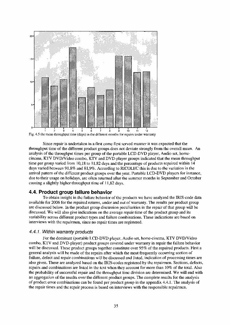
20

15

10

1 2 3 4 5 6 7 8 9 10 11 12

Fig. 4.5 the mean throughput time (days) in the different months for repairs under warranty

Since repair is undertaken in a first come first served manner it was expected that thethroughput time of the different product groups does not deviate strongly from the overall mean. Ananalysis of the throughput times per group of the portable LCD-DVD player, Audio set, home­cinema, KTV DVDNideo combo, KTV and DVD-player groups indicated that the mean throughputtime per group varied from 10,18 to 11,82 days and the percentage of products repaired within 14days varied between 91,8% and 81,9%. According to RICOLEC this is due to the variation in thearrival pattern of the different product groups over the year. Portable LCD-DVD players for instance,due to their usage on holidays, are often returned after the summer months in September and Octobercausing a slightly higher throughput time of 11,82 days.

4.4. Product group failure behaviorTo obtain insight in the failure behavior of the products we have analyzed the IRIS-code data

available for 2006 for the repaired returns, under and out of warranty. The results per product groupare discussed below. In the product group discussion peculiarities in the repair of that group will bediscussed. We will also give indications on the average repair time of the product group and itsvariability across different product types and failure combinations. These indications are based oninterviews with the repairmen, since no repair times are registered.

4.4. 1. Within warranty productsFor the dominant (portable LCD-DVD player, Audio set, home-cinema, KTV DVDNideo

combo, KTV and DVD-player) product groups covered under warranty in repair the failure behaviorwill be discussed. These product groups together constitute over 95% of the repaired products. First ageneral analysis will be made of the repairs after which the most frequently occurring section offailure, defect and repair combinations will be discussed and listed, indication of processing times arealso given. These are analyzed based on the IRIS-codes registered by the repairmen. Sections, defects,repairs and combinations are listed in the text when they account for more than 10% of the total. Alsothe probability of successful repair and the throughput time division are determined. We will end withan aggregation of the results over the different product groups. The complete results for the analysisof product error combinations can be found per product group in the appendix 4.4.1. The analysis ofthe repair times and the repair process is based on interviews with the responsible repairmen.

35

4.4.1.1. Portable LCD-DVD player

The dominant sections are the disk-drive mechanism (32,7%), the system control section(29,2%), the power supply unit (13,7%) and the information display section (11,3%). The observeddefects are predominantly general (indicating that the failure cannot be adequately described by onecode) (17,5%) or caused by failure of an electric component or module (52,3%). The dominant repairsundertaken are replacement of the failing part (56,1%) and the control of functions (15,2%). The mostfrequent combination of options is a failing disk drive caused by a failure of an electric componentwhich therefore is replaced (23,8%). Of all repairs undertaken on portable LCD-DVD players 98,4%was successful.

On average the repair of a portable LCD-DVD player costs about 25 minutes. This time ishighly variable between product types, repairmen estimate that for different types between 15 and 40minutes is needed, because of differences in the time needed to open the product, and fault types,because of the amount of parts collected on a small surface.

4.4.1.2. Audio set

The dominant sections are again the disk-drive mechanism, the system control section and thepower supply unit with 38,9 15,0 and 12,8% respectively. The defects classifications are failure of anelectric component (36,7%), general (24,8%) and no fault found (15,7%). The dominant solutions arereplacement (56,1%) and the control of functions (11,9%) or specifications (10,9%). The mostfrequently occurring combinations is a failing disk drive caused by a failure of an electric componentwhich therefore is replaced (16,4%). The success rate ofrepair on audio sets is 95,3%.

The time needed for the repair of an audio set is 30 minutes on average. This time is nothighly dependent on the type of failure and its repair. It is however highly variable, between 15 and45 minutes, among product types due to differences in the time needed to open and close the set.

4.4.1.3. Home cinema

The disk-drive mechanism is the most frequent failing section with 41,7% followed by thesystem control section (16,5%), general failures (12,1 %) and analog audio processing (11,6%). Themost frequently observed defects are defects of electrical components or modules (39,2%), no faultfound (27,0%) and general (17,5%). Replacement of product parts (52,6%) and the testing offunctions (20,1 %) and specifications (16,3%) are the dominant repairs. Again a failing disk drivecaused by a failure of an electric component which therefore is replaced (23,7%) is the most observedcombination. The success rate is 97,8%.

The average repair time of a home cinema set is roughly 30 minutes. This time is highlyvariable among different failure types, varying between 15 and 40 minutes. There is only minorvariation among product types.

4.4.1.4. KTV DVDlVideo combo

The dominant failure sections are the disk-drive mechanism (47,7%), the power supply unit(16,5%) and general (11,5%). The failures are a failing electrical component (47,5%) and no faultfound (29,1 %). The dominant repairs undertaken are replacement (52%) and the testing of functions(22,1%) and specifications (14,5%). The dominant combinations are a failing disk-drive mechanism(25,5%) or power supply unit (12,5%) which are caused by failing electrical components which arereplaced. The success rate for repair is 98,2%.

On average the repair of a KTV DVDNideo combo takes about 35 minutes. There is not a lotof variation among failure types or among product types. However there is a strong learning curvepresent for failures in the television section due to the technical nature of conventional KTVs and thedifficulty of finding the part that caused the failure on the first products. Finding this part becomeseasier with experience.

4.4.1.5. KTV

The most failing sections are the power supply unit (38,9%), the system control section(16,3%) and general failures (13,0%). The dominant defects observed are a defect electricalcomponent or module (42,8%), general defects (16,7%) and no fault found (15,4%). The undertaken

36

repairs are component replacement (54,1 %) and testing on functions (12,7%). The dominantcombination is a failing power supply unit because of defect electrical components which aretherefore replaced (23,6%). 96,4% of the repairs are successful.

The average repair of a KTV takes roughly 35 minutes. Not a lot of variation is presentamong product types or failure types. However, like for KTV DVDNideo combinations a stronglearning curve is present between subsequent repairs.

4.4.1.6. DVD-player

Four sections account for more than 10% ofthe failures each. These are the disk-drivemechanism (26,3%), the system control section (24,9%), the power supply unit (18,2%) and theremote control (11,5%). The most observed defects are a failed electrical component (36,0%), no faultfound (21,1 %) and general failures (20,9%). The most frequently undertaken repair actions includereplace ofthe component (53,3%) and testing on specifications (15,7%) or functions (13,7%). Themost observed combinations are a failing power supply unit (12,4%) or disk drive mechanism(10,3%) both because of failure of an electrical component which is then replaced. 96,4% of therepairs are successful.

The repair of a DVD-player takes about 20 minutes. There is not a lot of variation betweenproduct types or failure types.

4.4.1.7. An aggregation

As can be seen, most failures occur in just a few sections. This is not product groupdependent. The disk drive mechanism, if a product has one, is very vulnerable. Looking at otherproduct groups that are repaired this observation is confirmed. For VCRs the major section of failureis the tape-drive mechanism (84,1 %). According to the repairmen the moving character of therespective sections makes them vulnerable. Overall the disk-drive and tape-drive mechanism togetheraccount for 33,7% of the failures. Other sections frequently causing problems are the system controlsection (19,4%) and the power supply unit (14,8%), although general failures also occur regularly(10,9%). The overall ranking for defects is also in line with the above results. 30,6% is caused by afailing electrical component or module, 29,5% has a general cause and in 19,3% of the cases no faultis found. The undertaken repair actions are the replacement of a component (52,6%) and the controlof functions (18,5%) and specifications (10,5%). There is only one overall combination accountingfor more than 10%, this combination is, not surprisingly, the failing disk-drive mechanism because offailure of an electrical component which is replaced (12,2%).

The overall success rate of repairs is 96,9%, however it must be noted that the repairmen,based on their experience with the repairs, state this rate to be lower. This because they sometimesswap a failed repaired product with a product from cannibalization stock, this is not registered in thefigures and therefore seen as a successful repair while it is not.

4.4.1.8. Within warranty products: sales value distribution

Not every product that is returned is equally expensive and thus the costs for replacement orreimbursement or not equal for all returned products. This makes repair more profitable for someproducts than others. Here we have examined how the sales value of the repairs is distributed over thedifferent months in the year.

To obtain the distribution of the profitability of repair we would need the sales prices of allreturned products in 2006. This information was not available. Therefore the sales price distributionwas estimated based on the prices of several product types of each product group. The product typeswere drawn from the returned product types in 2006 and were checked on their representativeness forthe product group with respect to the sales prices with RICOLEC. With these prices average prices foreach product group were constructed. The returned products covered under warranty were classifiedin four and six levels based on the sales price information available. The distribution of the levels inpercentages of the total returns varies only slightly in the different months of the year. If four levels inthe sales price were distinguished the maximum spread in percentage of the total returns within onelevel was 13,2%. If six levels were used this number increased to 15,1 %.

37

4.3.2. Products outside warranty coverageHere we will discuss the frequently occurring failure sections and defects. The dominant

sections are similar to the repairs within warranty. The disk-drive mechanism (29,2%), the powersupply unit (20,7%) and general (17,9%). The observed defects do differ slightly from the defects inwarranty returns. The most frequently observed defect is still a failure of an electrical component ormodule (30,2%) and general defects are also frequents (18,3%). However wear out of a componentcausing low performance (20,8%) and mechanical breakages (13,9%) constitute important defects aswell.

The products that are repaired are repaired mostly by the replacement of worn out or failedparts (87,8%).The full results for the failure repair combinations of products out of warranty coverage processed bythe repair department can be found in Appendix 4.4.2.

4.5. Spare part inventory managementAs stated earlier, no registration of spare parts used is in place. In the past registration was

performed for sometime, but it was discontinued because of the constant errors made in theregistration. Still we can provide some estimates on the spare parts usage and the value of the spareparts. In 2006 for roughly €60000,- was purchased in parts, this includes all modules and parts of non­negligible value so also for instance remote controls that are sold separately. This excludes bulk partsas transistors or diodes, but their value is very small and can be neglected. These parts are notconsidered further in this project. In the IRIS-classification it can not be seen which part is used if areplacement is done. Therefore we will use estimates provided by the repairmen based on theirexperience during repair. They are also responsible for the inventory of parts, although they do notorder the parts, and therefore they have knowledge on which parts are in stock and used.

The repairmen estimate that about 70% of the components used are laser units. For 2006 anestimate of 2000 used laser units is made. In general about 10 to 15 types of laser units are used in therepair of products, these are only rarely interchangeable. The other component used frequently is asoftware-board (20%), which is a printed circuit board. There are numerous types of these boards,RICOLEC uses more than 20 types in their repairs, but not for all devices boards are available atRICOLEC. Lastly power supply units are used, but far less frequent (5%), often the power supply unitis incorporated on the software-board.

The repairmen estimate that they currently get 40% of their spare parts throughcannibalization of other products. However they are not able to give a funded estimate for 2006,because they are not able to recall how often they cannibalized products then. Sadly it was notpossible to determine whether a product was put in stock for cannibalization or in stock forsecondhand sale when it was decided that the product was not repaired. Therefore we do not knowwhat was put in stock for cannibalization directly. On the other hand we also do not know whatproducts were put in stock for cannibalization by the repairmen when a repair fails. Totally we can notgive any estimate on the cannibalization inventory, or its use in 2006.

Lastly an estimate can be given of the out-of-stock probabilities of spare parts. This figureindicates the percentage of times a repair can not be performed because no spare parts are available,neither in normal nor in cannibalization stock. This percentage is estimated by the repairmen to liebetween 2 and 5% of the total number of repairs. This includes only the repairs that normally areperformed.

4.6. ConclusionCurrently, most products are repaired within 10 days and in general the more expensive

products are repaired with high success rates. With a goal of the repair of a maximum total sales valueof the products within the maximum throughput time of 10 days it must be concluded that the overallfunctioning at the moment is not bad. However no guidelines are present nor followed. Thefunctioning is based solely on the experience of the repairmen, leaving multiple opportunities toimprove upon the performance besides the possibility to introduce decision rules in order to structurethe repair process. In the redesigns of the process in the subsequent chapters we will focus onforming decision rules that guarantee a high value of products repaired within the maximum

38

throughput time taking into account different possible supply situations, in terms of numbers ofreturns and the value of returns, RICOLEC can be facing in the future. With these rules it is tried toovercome the following shortcomings evident from this analysis

1. The selection of products for repair, thus which products to repair. Currently the time neededfor the different repairs is not incorporated in the decision whether to repair or not, which maylead to suboptimal allocation of repair time, since cheap but fast repaired products canpossibly be more profitable to repair than expensive but time consuming products. At themoment it is thus not clear whether the right products, from the viewpoint of money saved onreimbursements, are repaired. Also the information on the ease of repair which is gatheredduring the first product test before a product is included in the assortment is not used in therepair planning process, while this information can be of use in the planning of repairs.

2. The control of throughput time of the products sent to the repair department. Throughput timecurrently is not explicitly controlled nor considered when products are sent for repair,therefore the amount of products repaired late, although not high at the moment, can changedrastically under changing circumstances. This needs to be controlled in the redesigns.

3. In the current process no distinction is made between the returns on the maximum throughputtime whilst this differs between returns. For most returns, 70%, the failure to settle the claimwithin 10 days renders the repair of the product useless since it has to be monetarilyreimbursed anyway. For the other 30% no such strict number of days is present although athroughput time of 10 days is aimed for by RICOLEC, RICOLEC expects that whenthroughput times exceed 15 days these customers demand financial reimbursement.

4. With respect to the inventory management of spare parts the conclusion is that no realmanagement exists. However the money spent on spare parts is only a very limited amountand the results are, in the form of out of stock probabilities, acceptable. No guidelines todecide what products to stock for cannibalization are present.

5. Also the replace or reimburse decision motives are not insightful and this decision is largelymade to achieve customer satisfaction. However the cost associated with the decision optionsare not registered, nor taken into account.

6. Lastly no insight is gained in the failure behavior of product types that are not considered forrepair. The insight obtained in products that are repaired is not reported in a structuredmanner. Because of this the suppliers of RICOLEC cannot be informed about or heldresponsible for (poor) product performance.

The first three conclusions deal with the decision what to repair and what not to repair. The fourthconclusion deals with the decision what to cannibalize. The fifth conclusion focuses on the decisionwhether to reimburse or replace a product. Finally the last decision reveals the lack of insight in thequality of products that are not repaired.

Chapter 5 gives an overview of the different redesigns, which are then explained in moredetail in the Chapters 6 to 11.

39

5. Outline Redesign

The different redesigns try to overcome the shortcomings explained in the conclusion of thepreceding chapter. To do so the process, as displayed in chapter 2, is modified. The new model isdisplayed in figure 5.1. The test transition was added to the model, as indicated in the ellipse in thefigure. This indicates the possibility that a product is tested when it is not repaired to gain informationon the failure of the product.

The redesigns made for the problem can be divided into different parts, each covering anaspect of the process and each focusing on one of the decisions necessary in the process. We will, inthe redesigns discuss the decision whether to repair, the decision whether to test, to cannibalize andhow to settle the claim. We will explain the different parts in detail, explaining the reasoning behindthe proposed decision rules, in the subsequent chapters. In these chapters the research questions posedin Chapter 2 are implicitly answered.

In the model we assume that the decision involving repair is always taken before the otherdecisions as indicated in the flow model depicted in figure 5.1. With this the implicit assumption ismade that it is always more valuable to repair a product then to cannibalize it. This might not be thecase when the parts that can be used from a defect product are together more valuable than therepaired product. However it is expected that is will only very rarely be the case because everyproduct, when cannibalized, delivers only one and sometimes two parts. Also this assumptionimplicates that repair is found more important than testing a product. However if a product is repairedit is automatically tested. If a product is not repaired after all, the decision to test can still be taken.This sequencing of the decisions on the other hand greatly simplifies the problem and makes it easierto design implementable solutions.

The different parts of the redesign will be discussed in the subsequent chapters. Chapters 6 to9 will focus on the decision whether to repair or not, and present different redesigns focusing ondecision procedures that improve upon the present situation. With these redesigns an answer is givento the research questions on what and how much to repair. The shortcomings discussed in the firstthree conclusions discussed in section 4.6 are incorporated in the redesigns.

Currently the decision whether to repair a product is taken at intake. If the decision is to repairthen an attempt at repair is always undertaken. This creates a dilemma. On the one hand we have tomake sure products are repaired before they are due so we have to limit the amount of products sent tothe repair department, thus controlling throughput times. On the other hand we do want the repairmento be busy all the time, so we have to make sure there are always products to repair present at therepair department. To do so we have to make sure a lot of products are sent to the repair department,which contrasts the earlier requirement. In the current situation the throughput times are regulated bymeans of measures based on the number of days the eldest product is in inventory and products areprimarily in order of arrival although occasionally this order is not followed, why and on what base isunclear and not registered. Also the selection of products for repair is improved in the redesigns. Alast characteristic of the current situation is that products are placed in carts and cannot easily beaccessed individually when in stock, therefore decisions what to repair are taken on a cartlbatch basis.These characteristics will be looked into in the design of a solution. However, in all redesignscapacity is assumed to be given and limited. Limitations of capacity, which can occur from, forinstance, voluntary leave of employees or retirement, are only briefly considered when discussing theperformance of the different redesigns. Totally 4 different redesigns are considered. They arediscussed in order of increasing complexity, e.g. their deviation from current practice.

In Chapter 6, the first redesign takes the current situation and extends it by including productbased workload regulation, however without a fixed maximum capacity of the WIP, and a refinedbase for the selection of repairs. An extension of this redesign with priority rules, Redesign lb, is alsodiscussed. Redesign2, discussed in chapter 7 extends the first with a WIPcap, that makes sure no morethen a certain number of products is accepted, thus the WIP has a fixed maximum. This preventsproducts from being repaired too late. Redesign 3, discussed in chapter 8, differs from the previousredesign because it includes the possibility that products, after a first decision to repair, are notrepaired after all and the claims are financially reimbursed. Lastly chapter 9 will discuss the fourth

40

redesign in which products are accessed and scheduled individually at the beginning of each dayinstead of in batches upon arrival. The redesigns partly build on each other. For each redesign only thefeatures in which it deviates from the previous redesigns are discussed.

Finally Chapter 10 will focus on the test decision incorporating the sixth conclusion of section4.6 and answering the research question how to obtain insight in the failure of not-repaired products.Chapter 11 will discuss the cannibalization and replacement/reimbursement decisions, incorporatingthe fourth and fifth conclusion of the previous section and providing answers to the research questionsassociated with these decisions.

Chapter 12 discusses the settings of a simulation used to compare the first three redesigns forthe decision whether to repair a product or not. The results, together with analytical analysis will beused to judge which of the redesigns is best under which situations. This is discussed in chapters 13 to16.

Fig 5.l.: Redesigned flow model

41

6. Repair or not? Redesign 1: repair selection & throughput timecontrol

Currently the decision to repair or not is taken at intake. If decided to repair an attempt isalways undertaken. The sequence in which repair is undertaken is first come first served (FCFS),although some unclear priority rule is sometimes applied.

6.1. Redesign 1: RationaleThe current situation is the result of numerous years of experience. The decision procedures

used were not designed explicitly but are the result of a lot of small, unstructured, steps. Although thein the current situation already over 80% of the, usually more expensive, products is repaired on time,as was indicated in section 4.6, still the selection and control mechanisms used can be improved uponwithout changing the structure of the process. This redesign looks at the used mechanisms and tries toimprove and formalize them. For three mechanisms alterations are suggested. First for the regulationof the throughput time, second the selection of returns sent to the repair department. Lastly, inredesign 1b for the sequencing of returns in the Work In Process (WIP). The differences between thecurrent situation and the redesign are explained in the separate paragraphs. We will conclude with asynthesis of the different changes which completes the redesign and a discussion of the practicalchanges needed to implement this redesign.

6.2. Redesign 1: Throughput time regulation

6.2.1. Current: due date based WIP controlThe amount of work in process is regulated by the repairmen. If they observe that the

throughput time of the products to be repaired is increasing to beyond a number of days, around 13days, they tell intake to send less products to the repair department. If, on the other hand they observethat the throughput time of the product in the WIP is only a few days, around 3 days, they tell intaketo send more products. Which products are sent is detennined based on the value of a product,expressed in the cost price, which is calculated by adding RICOLECs costs to the purchasing price. Ifmore products are needed, in periods with fewer returns, some cheaper products are also sent and iffewer products are needed, in periods with more returns, only more expensive products are sent.

This method of regulation does not take into account the number of products in the inventory,only the number of days products have been in the inventory by looking at the entry date labelsattached to the carts by the collection department. Because the number of products per day varies thiscan lead to errors since the throughput time is determined by the amount of products in inventory andthe available capacity, not by the number of days the earliest received product is in inventory.Therefore we propose to control WIP based on the amount of products in the WIP and capacity.

6.2.2. Redesign 1: Product & capacity based WIP controlSince all work that is sent to the repairmen needs to be repaired because once the decision to

repair is made it cannot be changed we can only directly control the average throughput time bycontrolling the amount of work in the queue, thus the amount of work sent to the repairmen. In thisredesign a CONWIP like strategy is chosen, however no strict maximum is set for the queue length,also named WIP.

The throughput time of a product consists of two main elements. The processing time, whichis the time necessary for repair, and waiting time, which is the time the product is in the queue. Theprocessing time is generally very small compared to the waiting time. The waiting time consists oftwo main components; the time until the product presently under repair is processed, which is theremaining service time, and the total processing time of all products in front of the product in thequeue. However, since on average 2 to 3 repairmen are working and the average repair time is around30 minutes the remaining service time averages about 5 minutes and thus is very small compared tothe time needed to process all products in the queue, since in the queue multiple days of work arewaiting normally.

42

We do not know the total processing time of the waiting products since their processing timesare variable. We only know the mean processing time, which deviates between product groups anderror types, but overall equals 30 minutes. Based on the information on the processing time acquiredthrough the interviews with the repairmen we assume the repair times of a random product to benormally distributed with mean, IIp =30 minutes, and standard deviation, ap=5 min (assumed basedon the information on the spread in repair times given by the repairmen), and that processing times ofproducts are independent from each other.The average minutes work in process in the queue now becomes:

IiMWIP = n * lip (6.1)And the standard deviation becomes, in minutes:

aMWIP = Vn * a p (6.2)With:n =number of products in the WIP, excluding products under repairMWIP =minutes work in process

Capacity consists of the personnel, repairmen, available to repair products. Howeverrepairmen do not only repair products. They also need time to transport products and control batches;this is assumed, based on the interviews with the repairmen, to be a fixed 2 hours per day in total.Next to that they also need time to cannibalize products to obtain parts. Capacity to repair andcannibalize then is defined as:

CAPrep,x = Cf.f,'f k ij ) - 2 x x (6.3)

Where:CAPrep,x =capacity for repair and cannibalization at the repair department in the next x working days(hours)i =days, from 1 to xx =maximum throughput time of products set by RICOLEC, in daysj =repair men, from 1 to 4kij =number of hours repair capacity per worker per day

The second factor, 2 x x, displays the hours needed for transport and control of batches in x days,these need to be subtracted from the capacity.

Cannibalization for parts is mostly performed during the repair of a product. If a repairmansees the needed part is unavailable he takes a product stocked for cannibalization and gets the partfrom that product, after this he continues with the repair of the to be repaired product. This time is notincluded in the repair time per product. Whether cannibalization is needed is not known in advance.Cannibalization is performed in about 40% of the cases where a part is required, which is in about40% of the repairs. Therefore cannibalization is needed in 16% of the cases. Cannibalization,according to the repairmen, requires 15 minutes per attempt. We have to subtract this capacity fromthe total capacity available for repair, since both tasks are executed by the same personnel. Includingthis, the probability that on a newly arriving product repair is started within x days then becomes,under FCFS service discipline:

P(MWIP < (CAPrep,x - 0,16 x n x 15))With:CAPrep,x =the capacity for repair of warranty products in the coming x days

(6.4)

RICOLEC aims for a throughput time of 10 days for all products. In order to be 95% sure anewly arriving product is repaired within 10 days the WIP should be kept under the level of:

n x IIp + Z(O,95) x vn x ap = CAPrep,10 - 0,16 x n x 15With:Z(O,95) =Standard normal distribution value for 0,95

43

(6.5)

Now, if the WIP level for some reason rises above n chances are larger than 5% that not all productsare repaired within 10 days. The WIP level number includes warranty and out of warranty products.

The number of out of warranty repairs is not controlled in this research; still capacity isneeded for these returns. Therefore in the WIP level room has to be made for out of warrantyproducts. The amount of room can be determined from the analysis in chapter 4. We can relate thenumber of out of warranty repairs generated in 2006, according to the repairmen no large changeshave taken place since 2006 and are not expected in the future, to the total number of returns andassess the needed capacity for out of warranty returns.

As followed from the analysis in chapter 4. Out of warranty returns accounted for 4 to 6,3%of the returns in the different months. The percentage of non-warranty returns repaired is 50,5%. Thisfigure was quite robust over the year. Times needed for inspection are very small and can beneglected. The capacity needed for repairs not covered under warranty is dependent on the totalnumber of returns. On average 5% * 50,5% = 2,5% of the total returns each week need to be repairedas out of warranty returns. In the different years on average between 300 and 400 returns arrive perweek. We reserve capacity for 2,5% of 400, thus 10 products per week, as out of warranty returns.Therefore the WIP level of warranty returns needs to be kept under n-l0 products.

6.3. Redesign 1: What to repair?: Profitability of repairIf capacity was unlimited and free it should be best to repair every product submitted under

warranty if the transportation and part costs are neglected. However capacity is neither unlimited norfree. We can only repair part of the returns, but not all returns are equally interesting to repair.Therefore we need to establish a measure for the attractiveness of repairs. Now this is measured basedon the cost price of a product and does not include other factors influencing the attractiveness ofrepair like, the time needed for repair and the spare part costs.

A new measure was developed. This measure is based on the costs and benefits of repair. Forproducts within warranty the benefits of repair for RICOLEC are the avoided costs of replacement orreimbursement. The costs of repairing a product are a function of the spare parts used, the cost fortransportation of the repaired product back to its submitter and the time necessary for repair. Theattractiveness of repair depends on the repair time necessary since time is a scarce resource. Thereforethe attractiveness of repair is expressed per unit of repair time. Mathematically the attractiveness ofthe repair of a specific failure type on a specific product type per unit of repair time can be defined as:

A .. - MineCreim,iCrepl,;)-Css,ij-Ctr,ki

lJ - tr,ij(6.6)

With:i = index indicating product typej = index indicating error typek = index indicating type of transport needed for a product from RICaLEC to the customerAj = attractiveness of repair of a specific error on a specific product type per unit timetr,ij= average time necessary for the repair of a specific error type on a specific product typeCreim,i = cost for reimbursement for a specific product typeCrepl,j = cost for replacement for a specific product typeCss,ij = cost for spare parts for the repair of a specific error type on a specific product typeCtr.k.i = cost of transportation of the product to the end user after repair for a specific product typetransported by a specific type of transport.

The different variables are not all known at the moment due to data limitations. But all caneither be gathered or measured by RICOLEC without great effort or cost. The time needed for repairof the product is unknown beforehand but can be estimated during the testing of the product which isdone before a product is put on the market. This testing is done by an experienced technician. Duringthe test he opens and closes the product and examines the structure of the components. Since the timeneeded for repair is predominantly determined by the time needed for opening and closing the productand the structure of components, he can estimate fairly accurately the time needed to perform a repairof a certain error. This is then done on product type error type combination level and therefore

44

eliminates the variability between product types and/or error types. During the first repairs, ifundertaken, the estimated time can be corrected.

The measure does not incorporate the probability that cannibalization is used nor theprobability that repair fails. This because no product or product type specific information is present onthese issues and using overall averages would not discriminate between results.

To be able to compute the profitability of repair level the error type needs to be known whenthe product arrives. The error type needs to be extracted from the complaint description given by thesubmitter. However, submitters do not always provide information and thus the type is not alwaysknown beforehand. If the error type is unknown the weighted average spare part costs and weightedaverage repair time for a product type can be used so the measure is still usable.

6.4. Redesign 1: SynthesisWhen the WIP level on which it is 95% certain all products are repaired on time is known we

can regulate the WIP level by influencing what is sent to the repair department for repair the WIPlevel around which the WIP is regulated is termed the WIP control level. Control can be done bysetting the profitability of repair level at intake. Then if the WIP level is higher or lower than thecontrol level the profitability of repair level at intake can be changed. However, due to the uncertaintyin the arriving of products, the effect of a change in this level cannot be predicted beforehand. Weonly know that in general, if we raise the level fewer returns will be admitted and if we decrease thelevel more returns will be admitted. We have to observe the effect of the change and after observation,if necessary, adjust the level once more. The observation period has to be set. Since the returns are notdistributed evenly over the week we propose to set the observation period on once a week toincorporate the variations in effect in the different days. Due to the unknown effect of theinterventions the WIP level will vary a lot on the high and low side of the control level. Therefore,when the WIP level is controlled around the limit discussed above, a lot of products will not berepaired within the required times, rendering the repair useless, and the overall value of the within­time repairs will be low. By setting a lower WIP as control level the amount of products repaired latecan be controlled.

By setting a lower control level the WIP, with the variation in arrivals, can be kept under themaximum level during the year, thus preventing products from being repaired too late. The downsideof a lower WIP level is that the probability that repairmen are out of work increases and thus fewerrepairs will be performed. Exactly what the influence is of lowering the level will be determined inthe simulation.

6.5. Redesign 1b: Priority rulesCurrently RICOLEC aims for a throughput time of 10 days for all products. However this

target is not equally important for all products. If a product is not repaired within a certain amount ofdays the repair becomes useless in that still financial reimbursement needs to be paid to the submitter.For 70% of the products this period is 10 working days, whilst for 30% it equals 15 working days,although it is expected that the percentage of products requiring a throughput time of 10 days willincrease in the future. The maximum throughput time is set by the submitter of the product and doesnot differ between products from the same submitter. This implicates that when a certain product isnot repaired within 10 days it can better be a product that should be finished within 15 days since thenthe late repair does not lead to reimbursement costs. To influence this possibility priority can be givento certain products. To be able to do so batches of products should hold only either priority or non­priority products. Because priority products arrive with different logistic service providers than nonpriority products, this is easily arranged by the collection department.

Currently some priority at times is given to the 70% of products that need to be finishedwithin 10 days, but it is unclear on which basis and under which circumstances this is done. We willtherefore assess the influence of some priority rules. At RICOLEC, as explained, two groups ofproducts can be discerned. The first group needs to be repaired within 10 days. For the second groupthis maximum is 15 days. A level of priority should also be assigned to out of warranty products sincethey need to be processed by the same repairmen. RICOLEC treats these repairs the same as non­priority warranty repairs. A throughput time of 10 working days thus is desirable, but 15 days is the

45

maximum. Therefore it is logical to give out of warranty repairs the same priority as non-prioritywarranty products.

The goal of the priority rule is to make sure that the products that are not repaired within 10working days are of the second group, provided the repair takes place within 15 working days.However due to the batches in which products are placed we can, without altering the manner of stockkeeping, only assign priority to a batch of products. A batch contains products with the same intakedate and the same maximum throughput time, thus with the same priority. We can therefore onlyprioritize products based on their entry date and maximum throughput time.

The used rules give some priority to certain products over other products. When priority isgiven to priority products they can upon entering 'skip the queue' a number of places to get in front ofa number of non priority products. This increases the probability that they are repaired on time, but itdecreases the probability that the skipped, non priority products, are repaired within 10 days. Thissince, as was explained in chapter 3, the average throughput time over all products will remain equalregardless of how many days priority is given to certain products. Therefore the total WIP needs to becontrolled as well as was explained in 6.1.2. The effect of the priority rule in causing an increase inthe percentage of product on time depends on the WIP level upon entering of a product and thenumber of days priority given to a product. However a first, small step to achieve higher performanceon priority products can be obtained by a priority rule stating that priority products with a certainentry date are always repaired before non-priority products with the same entry date. Here thus apriority rule based on the entry date is used. This principle can be extended and priority can be variedin the number of days priority products get entry date priority over non-priority products. Forexample, priority products with an entry date of 20 April are repaired before non-priority productswith an entry date of 19 April if priority products receive] day priority over non-priority products. Inthe simulation 1 and 5 days of priority are tested. 5 days priority leads to the same sequence as earliestDue Date scheduling since the difference in maximum throughput times between priority and non­priority products is 5 days. Earliest Due Date scheduling minimizes the maximal Due Date expirationand forms a starting point for the minimization of the number of orders with Due Date expiration(Bertrand et aI, 1998) as was explained in chapter 3.

The effect of a priority rule is strongly dependent on the number of products receivingpriority. This number is dependent on the number of returns from specific customers which cannot becontrolled by RICOLEC. Therefore the effect of using a priority rule cannot be controlled byRICOLEC.

6.6. Redesign 1: Practical implicationsTo implement this redesign, both variants of it, no big structural, physical changes are needed.

The decisions are made at the same points in time as in the current situation and the decision optionsalso remain the same. The only changes made are in the basis for the decisions, thus in the dataneeded to make the decisions. We will discuss them in the order in which they were discussed above.

To regulate throughput time the amount of products in the WIP needs to be measuredperiodically. Also the link between the WIP level and the input level, as expressed in the profitabilityof repair, for the repair department has to be made explicit. Lastly a period to update the input levelbased on the WIP has to be set, preferably once a week.

To implement the selection of repairs based on the profitability information is needed on theexpected spare part and transport costs in addition to the cost price also the return needs to beaccompanied by a failure description from which the error type can be discerned. Lastly the timeneeded to repair the error is needed. All this information can be gathered from different sourcesincluding the sales department, the pre-market launch product test and the submitter. The sales price,that equals the cost for reimbursement, is known within RICOLEC, the repair time and spare partcosts can be estimated from the pre-market launch test. The transport cost are determined by themanner of submitting the product and thus known upon arrival. Lastly RICOLEC needs to demandthe accurate descriptions of the observed failures from their customers submitting the products, whichmight be difficult to realize. If a product is lacking a detailed failure description the average repairtime and spare part costs for that product can be used for the calculation of the profitability of repair.

To implement the sequencing procedures for the products in the WIP only the stock keepingof the carts in the inventory should be altered to make sure repairmen can take the right cart. It should

46

7. Repair or not?, Redesign 2: Maximum WIP level extension

7.1. Redesign 2: RationaleIn the first redesign the WIP level needs to be controlled on a level below the 95% certainty

WIP level at which timely repair is highly probable to prevent products from being too late. However,as stated, this may lead to fewer repairs. In order to increase the WIP level for control and limit therisk on useless repairs an upper limit on the WIP, a WIPcap, can be set as is done in CONWIPsystems. This limit serves as a maximum on the WIP level, no more products are admitted when themaximum is reached.

7.2. Redesign 2: WIPlevel control with WIPcapIf a WIPcap is installed this has the following consequences for the admission of the products.

If the WIPlevel is below the cap products are admitted as in the first scenario. If the limit is reachedno products are sent to the repair department anymore. This contrasts the first redesign whereproducts were admitted only based on profitability of repair which was set based on the WIP once aweek allowing the WIP level to rise above the maximum. Now the WIP level for control can be set atany level, thus higher levels as in the first redesign, since the WIP level can never exceed themaximum level at which the cap is set. In this way more repairs can be performed. However, there isa drawback to this redesign. When the cap is reached no more products, thus also no more verylucrative products, will be sent for repair but instead less lucrative, already admitted products arerepaired. This makes sure that, in hindsight, it is certain it would have been better to repair differentproducts. The consequence of this error is higher when the WIP limit is closer to the control level forthe WIP since then the cap will be reached more often.

The height of the cap can be set based on the probability that a newly arriving product isrepaired late when the limit is reached following:

n x IIp + Z(O,95) x,,;n X up = CAPrep,x - 0,16 x n x 15

We will use a probability of 95%.We will examine the effect of different WIPcontrollevels with the WIPcap in the simulation.

(7.1)

7.3. Redesign 2: Practical implicationsIn addition to the first redesign now the height of the WIPlevel should be monitored at the

intake of every new return, instead of once a week as in the first redesign, to examine when theWIPcap is reached. If the cap is reached it should be made sure no more products are sent for repairby the employees at intake.

48

8. Repair or not?, Redesign 3: Final decision at the repairmanIn this redesign the decision whether to repair a product can be altered after intake. At intake

a first decision is made and products are sent to the repair department. Then when a product is takenby a repairman, in contrast to the previous redesigns in which repair was always attempted on a sendproduct, the final decision is made whether the product is repaired or not. Products can only beaccessed in carts. The carts are processed in a first-come-first-served order.

8.1. Redesign 3: RationaleLooking at the first two redesigns, both discussed options to control the timely repair of

products have some drawbacks. These are mainly a consequence of the fact that the decision to repairhas to be taken at intake and repair has to be performed when the decision is made. If the finaldecision to repair a product is postponed until the moment a product is taken by a repairman we cananticipate on this. Then if a product is either already too long in the WIP or if a product has a lowprofitability of repair and its repair would prevent the timely repair of another product it can bedecided not to repair a product, so useless repairs can be avoided and it is controlled that the moreexpensive products are repaired. This decision is displayed to the repairmen when he looks up therepair in the system before repair. This redesign adds a control on the WIP to the first redesign. Belowwe will first discuss the WIP control mechanism in place in this redesign. Lastly the practicalimplications of the redesign are discussed.

8.2. Redesign 3: WIP control mechanismIn this redesign not all work in the queue has to be repaired. However if it does not have to be

repaired it still needs to be handled. A repairman has to take the product, look up whether it should berepaired and place the product on the right shelf if it should not be repaired. It is estimated, based onthe task description of a repair that this takes 5 minutes per product.

Because of the possibility to not repair a product even though it was sent to the repairdepartment we have an extra control for the throughput time. If too much work is in the queue or theproducts have exceeded their maximum throughput time, some products are not repaired and thequeue becomes shorter. The admittance of products to the repair department therefore becomes lessinfluential, since variations in the WIP caused by the arrival process (that are only known inhindsight) can be corrected by not repairing products. However this correction still costs time, makingthe first selection needed.

Throughput time is regulated by setting a profitability of repair level at intake and a level atthe repairmen. The level set at intake can be altered based on the WIP level. This level helps toregulate the admittance of products to the WIP. The level set at the repairmen also needs to be basedon the amount of products in the WIP but serves to control the time within which the admitted repairsare processed, thus the flow out the WIP. Of the work in the queue the profitability of repair is known.

The average waiting time of a product when admitted to the repair department becomes, withfirst come first serve service:

n x (( 1 - PR) x J1.np + PR x J1.p)

With:n =number of products in the queuePR = part of products in the queue that is repaired (0::; PR ::;1)J1.np = average processing time for not-repaired productsJ1.p = average processing time for a repair

(8.1)

In this formula n is influenced by the Aij set at the product intake whilst PR is determined by the Aij

set at the repairmen and the probability a product has waited longer than its throughput time in thequeue. By regulating both these levels we can control the waiting time and thus the throughput time ofthe repaired products.

49

8.2. 1. Profitability of repair at intakeThe profitability of repair at intake can be regulated around a control level for the WIP in the

same manner as in the first redesign. This manner minimizes the expected deviations in the WIP,provided the assumed value distribution is correct. Although the time needed for products thatexceeded their maximum stay is a lot shorter, 5 instead of 30 minutes on average, then in the previousredesign, still time is needed for the handling of a product. The amount of times this needs to be donelimits the amount of repairs that can be done. This amount is related to the WIPlevel used for controlas in redesign 1. In the simulation different levels for the control of the WIP are examined.

8.2.2. What to repair: profitability of repair at the repairmenTo control the throughput time of a product we can decide not to repair a product when the

product is taken by a repairman. There are two reasons to decide not to repair a product after all. Thefirst is that the product already has a throughput time larger then its maximum, rendering its repairuseless. The second is that repairing a product can prevent, due to the time restrictions, the repair ofanother, more profitable, product.

For the first reason the control is simple, since it only depends on the throughput time of theproduct. If it is larger then the set maximum throughput time no repair should be undertaken.

For the second reason the profitability of repair of all products in the WIP and the totalamount of products in the WIP is important. As long as the WIP level n < N no products should notbe repaired and thus Aij at the repairmen should be O. If n>N then this is different and an extraselection needs to be made at the repairman.

If all products need to be repaired WIP should be kept under a certain level as in Redesign 1and 2. This level can again be calculated by:

N x IIp + Z(O.95) x.,fN X up = CAPrep•x - 0,16 x N x 15 (8.2)

Then if the number of products in the queue is larger than N some products in the queue should not berepaired to make sure the last admitted product has a high, 95%, chance of finishing on time. It canbe that only late products should not be repaired. Therefore these need to be subtracted from the total.Then if more products should not be repaired, this number of products can be found by solving forPR:

(n - p) x (( 1 - PR) x Jlnp + PR x Jlp) = N x Jlp

With (in addition to above):n = number of products in the WIPp = number of late products in the WIP

(8.3)

Then knowing PR the number of products that should not be repaired but handled, h, from the WIPcan be calculated by (n - p) x (1- PR) = h. Now we can then select the profitability of repairsuch that h products in the WIP have a profitability lower than the selected level.

We assume that the standard deviation of the waiting time is equal to the standard deviation inredesign 1 and 2. This based on the fact that we will repair less products, which lowers the totalstandard deviation for the repaired products, but on the other hand we will not-repair more products,which adds to the standard deviation. Since both deviations are not known perfectly the effect on thetotal standard deviation can only be assumed. We assume the effect is zero.

8.3. Redesign 3: practical implicationsIn addition to the changes needed for the implementation of redesign 1 some extra changes

need to be made in practice.The addition of an extra decision with two options, repair or not, leads to a structural change

in the process. The needed calculations can partly be performed based on the information alsonecessary for the first redesign. In addition it is necessary to monitor the products and their waiting

50

times in the WlP, this needs to be monitored every time a product is added to or taken out of theWlP. The calculation of the waiting times can easily be done by subtracting the day of entry for thecurrent day for all products in the WlP. The calculations have to be done every time a new product istaken by a repairman.

Practically a repairman needs to have a place where not repaired products can be stored.Furthermore it needs to be specified how these products are further processed and by whom. Lastlythe repairmen and other involved personnel the new process should be explained so that they becomeconfident in working with it.

51

9. Repair or not?, Redesign 4: Individual product scheduling

9.1. Redesign 4: RationaleThis redesign extends the previous redesigns by adding the possibility to determine the

sequence of repair of products in the queue based on their individual characteristics instead of inbatches with the same priority level and due date. In addition this order can be chosen after it isknown which products have been sent for repair, this in contrast with the previous redesign where theorder was determined by the batches and determined when a product was sent to the repairdepartment.

In the previous redesigns a product is only not repaired if it either has a too low value or itswaiting time is too high. The waiting time is not based on the value of a product so it can be that veryexpensive products are not given sufficient priority and thus exceed their maximum waiting timewhilst cheap products do finish on time. Although the third redesign reduces this possibility, since itprovides for the possibility of not-repairing cheaper items to make sure more expensive products arerepaired it can still happen when the WIPlevel is large. This redesign prevents this from happening.

First the principle of individual product access and queue priority will be discussed. After thiswe will discuss the incorporation of individual access into redesigns land 3. In the second redesignWIP is always kept below the WIPcap rendering individual selection useless since all products can berepaired within the maximum throughput time. The discussed priority rule replaces the priority rulesdiscussed within redesign 1 earlier.

9.2. WIP processing: Individual product access & priorityIf we can select products to repair from the WIP based on their profitability of repair, we can

choose to repair more profitable products before less-profitable products since this is more profitable.We could simply pick the product with the highest profitability of repair from the queue each time arepair is picked. However then it could be that products that are in the WIP for only just one day arepicked before products already in the WIP for nine days. This might lead to suboptimal practices sincea lot of products are not repaired within 10 working days whilst others are repaired the first day.

This problem can be overcome if the optimal sequence of repair for all products in the WIP isknown so that the products that should be repaired next can be taken from stock. The optimalsequence however can be influenced by two parameters unknown beforehand. The first is that thesequence might be dependent on the products that will arrive within the time it takes to process theproduct scheduled for repair in the queue. However it is expected that this will only happen veryrarely because of the considerable WIP already present at the repair department at any time. Thereforethe probability that the optimal sequence for the period will change if the arrivals were knownbeforehand is very small and can be neglected. The second is that the time to process the scheduledproducts is unknown, whilst this time influences the time left for the other products and can thusinfluence their optimal sequence. It is not sure the products scheduled in a certain period are indeedrepaired in the period, since processing times are variable. To make sure the repairmen have enoughwork the number of products taken from stock should be larger then the periods work. Left overproducts after the period can be used in the calculation of the next sequence again.

Because products are handled individually the handling time, which is needed to take theproducts from stock and place them in the right places after processing, can be specified per product.However handling time is unknown and dependent on the manner of stock keeping. If products are alleasily accessible this figure will be low, if they are hard to reach it will be higher. In the first tworedesigns, for the handling of the batches a total of 2 hours per day is used. When on average 34repairs are carried out, which is the average number of repairs done in a day, this comes down to 3,5minutes of handling time per product. This redesign, it is expected, can therefore only improve uponthe previous redesigns if the handling times are lower or close to 3,5 minutes. Else the possiblebenefits obtained by repairing the right products are offset by the increase in handling time whichleads to the repair of fewer products, provided the repairmen take the products from stock.

52

The optimal sequence of repair of the WIP is then dependent on the due date of eachindividual product and the revenues, which is the costs of financial reimbursement, which are madewhen a product is not repaired on time. Due dates should be set based on the maximum throughputtime of a product.

The optimal schedule can then be found by adapting the algorithm of Hodgson-Mooredescribed in the third chapter to the current situation. The incorporation of the algorithm in redesign Iand redesign 3 is discussed below. It is uncertain an adaptation providing the optimal sequence for ourspecific problem situation can be made, as becomes evident from the discussion on this problem inchapter 3. In this report this will not be tried due to time limitations.

9.2. 1. Redesign 4a: Incorporation of individual scheduling in redesign 1In redesign I the value of the products that are not repaired on time is not controlled. By

introducing the individual scheduling this can be regulated and minimized.The Hodgson-Moore algorithm in its base form needs to be applied as follows:

1. All products need to be ranked according to their due date with the most recent due dates first.2. For every product the start time should be determined based on the average repair time

needed for the specific repair3. If the starttime plus processtime of a product is smaller then its due date for all products this

is the optimal sequence.4. If a product is late it should be examined whether the least lucrative product, based on

profitability of repair, with a larger processing time then the late product in the queue is lesslucrative than the late product.

5. If such a product is present it should be taken out of the queue and placed after the lateproduct.

6. Now repeat step 3 until all products are considered, products that are already placedbackwards are not considered.

This algorithm does not provide an optimal sequence in our situation since the assumptions,ego equal weights for products, discussed in chapter 3 are not met. However it is expected that anadaptation of this algorithm can be made that can be used as a heuristic to find close to optimalsequences for the situation under study.

The adapted algorithm should be used to calculate the optimal sequence once a day due to thetime consuming calculations that limit the use of calculation of the optimal sequence before eachrepair. Then the products that come first in the sequence are taken from stock. The repairmen onaverage repair the products scheduled for one day, and therefore should take a certain amount ofproducts from stock. However to prevent them, when they work faster, from being out of work, weshould take more products then the products scheduled for that day. Since we assumed the repairtimes for the products to be normal distributed with an overall mean of 30 minutes and a standarddeviation of 5 minutes, we can determine how large the probability is that a number of averageproducts is repaired in a day. To be 95 % sure that the repairmen will not finish all products takenfrom stock in one day we need to determine the number of products taken from stock. This can bedone by solving for the number of products:

n X 30 - Z(O,95) x..fii x 5 + n X th = CAPrep,l - 0,16 x n X 15

In which:n = the number of productsZ(O,95) = standard normal distribution value for 0,95

CAPrep,l = capacity the coming dayt h =time needed to take one product from stock

(9.1)

Then the first n products of the calculated sequence need to be taken from stock and be repaired inorder of the optimal sequence. If not all taken products are repaired the left over products do not have

53

to be placed back in stock, until it is certain they are not in the first n products of the optimal sequencethe next day. This to prevent the unnecessary handling of products.

9.2.3. Redesign 4b: Incorporation of individual scheduling in redesign 3In redesign 3 the processing of products beyond their due date is partly regulated by the level

at the repairmen. However this only functions if the WIP is kept within certain range of the limit. Toprevent lucrative products from being late when WIP is outside this range, individual access can be ofuse. The procedure to be developed should be applied analogous to the procedure discussed for thefirst redesign in 9.2.2. The only difference is that products that are late or of which the profitabilitylevel is to low are not repaired and their claims are settled by the collection department. Thepossibility that on time products are not repaired influences the number of products that need to betaken out of stock in the beginning of the day. Still n x 30 minutes should be taken from stock,however products that will be handled need to count for 5 minutes of work instead of their processingtime. It is known how many products will be handled, so the number of products taken from stock canbe adjusted to make sure n x 30 minutes of work for the repairmen are taken from stock. Anotheroption that can be looked into is to only take products from stock that need to be repaired. Productsthat need to be handled because they have exceeded their stay can then be handled by otheremployees, eg employees from the collection department. This creates more capacity for repair.

9.2.4. Comparison models and priority rulesAlthough the above stated modeling of priority among products is comprehensive and is

expected to lead to close to optimal results with respect to the selection of enough and the rightproducts for repair, it is questionable how much better it performs compared with the previousredesigns. The fourth redesign however cannot be simulated like the other three redesigns, since theredesign first needs to be developed. The expectation is that the decision procedures for this redesignin the form of a model can be developed and implemented however the development andimplementation is not done in this project due to time limitations. Now if the expected benefits arelarge, RICOLEC can choose to develop the model. We will assess the possible impact based on theupper boundaries on performance and the performance of the previous redesigns.

9.3. Redesign 4: practical implicationsTo implement this redesign in addition to the changes needed for the first/third redesign, the

manner of stock keeping at RICOLEC needs to be drastically changed. All products need to be madeaccessible individually. Then a placement system needs to be developed so it is known whereproducts are in stock so that they can be retrieved easily. The products have to be placed in the stockby the employees that take the products in and be retrieved by the repairmen or other personnel beforerepair.

Besides this it is necessary to continuously keep up to date information on the products instock, since this is necessary to calculate the optimal sequence.

One increase in risk inherent in the individual handling of products needs to be mentioned aswell. Individual product handling increases the risk of product damage since it is much easier to dropan individual product than a full cart.

54

1o. Testing products

10.1. Why testing productsIdeally you would have full knowledge on the performance of all the products you have sold,

since this knowledge can be useful in the development or purchase of new products Thus, if thisknowledge was obtainable at no costs, you would like to know what the failures on all incomingproducts were so that full knowledge on the failures can be reported to your supplier and used toprevent problems later. For products that are repaired registration of the error is 'free' because repair,which incorporates the actions taken during testing, is undertaken. However for products that are notrepaired this knowledge is not free since tests have to be performed to gain it, these tests are estimatedby the repairmen based on their knowledge of the products to take 15 minutes per product on average.However by sampling the returned products knowledge can be gathered on the failure behavior of theproduct types without testing all products. The more products are sampled, the more precise theobtained knowledge is.

RICOLEC wants to filter out the dominant failures for each series of each product type. Aseries constitutes an order of a certain product type at a supplier, a series accounts for between 100and 2000 products. RICOLEC expects the failures to be dependent on the series, since different seriesare manufactured on different times with possibly different quality, and therefore wants to test onseries level Upon return it is known to RICOLEC from which series a product is. The occuringfailures need to be classified during the testing of returned products.

The testing is done on IRIS code level. The section code and defect code should be combinedinto one result. The test thus leads to one classification for the failure section and defect code together.

10.2. How many products to testWhen 2 or more tests are performed, we can calculate boundaries for the probability that a

specific failure type, thus a specific combination of a section and defect code, occurs. The lowerboundary states that the probability is not lower then a certain figure and the upper boundary states itis not higher then a certain figure, both with some confidence. Therefore to set the boundaries aconfidence level, a, needs to be specified by RICOLEC. The lower boundary of the probability, Pmin,

is then calculated with:

(10.1)

With:Za = Standard normal distribution value for confidence level ax = number of occurrences of section-defect code combination in the tested productsn = total tests performed on specific product series up till nowPmin =minimal probability on the occurrence of a specific section-defect code combination for the

product series

The upper boundary, Pmax, is then calculated with:

(10.2)

With (in addition to above):Pmax = maximum probability on the occurrence of a specific section-defect code combination for theproduct series.

Since the tests are done on different products the tests are mutually independent, which is prerequisitefor using the normal distribution.

55

Now the more products are sampled, thus the larger n, the smaller the difference betweenPmax and Pmin becomes and thus the more precise the knowledge on the probability on a specificfailure type becomes. RICOLEC now has to specify a degree of precision expressed as an interval ofwidth Pmax - Pmin. This interval can be calculated after every test and the sampling can stop whenthe specified precision is reached. However to avoid for the possibility of endless testing because thedegree of precision is never reached, a maximum on the number of tests needs to specified as well.

To give an indication, using a confidence level of 85% and an interval width of 0,20 theinterval width is reached after 20 to 30 tests depending on the probability of occurrence of the failuretype.

Because it is desirable to have the information of the failures as quickly as possible the testsshould be performed on the first returns of the product despite the fact that this is not a randomsample, which is desired (Cooper and Schindler, 2003). This since some failures might beoverrepresented in the first returns, because they generally occur shortly after purchase (e.g. usershaving problems installing the product and sending it as failure because of this).

10.3. Capacity needed for testingIn order to get an idea of the amount of time needed for testing products each week we have

calculated a rough estimate of the number of tests needed each month. The estimation of the numberof tests should be done on a week-level. Unfortunately the necessary information was only availableon month level. An estimate of the number of tests required in each month was determined byfiltering out all product types the types for which less than ten returns, to account for overestimation,were received until the beginning of 2006. For these types the first twenty returns in 2006 weredetermined. This led to an indication of the number of tests that should have been done in 2006. Thisestimate was based on the number of twenty tests per product type, which is probably slightly lowerthen the number of tests needed per product series. Totally 934 tests (including during repair) shouldhave been needed, with a minimum of 56 and a maximum 141 tests per month. This figure probablyunderestimates the number of tests needed since it does not incorporate multiple series per producttype, whilst testing needs to occur on series level. Comparison of the number of tests needed in eachmonth and the total number of returns showed no constant relation. Therefore we cannot accuratelypredict the number of tests needed based on the number of returns received.

The time needed for inspection is determined by the depth of failure analysis desired byRICOLEC. The desire is to classify the failure section and the defect mode. The time needed for thisis a subset of the time needed for the repair of a product since it involves the same steps. The producthas to be connected and the complaint needs to be checked. Than, in most cases, the repair man needsto open the product to establish the failing component and the defect. Lastly he should close theproduct again. As stated, it is estimated that on average 15 minutes are needed to perform a test on aproduct.

Therefore, since only a limited number of products need to be tested, 934 out of 21000, withan average time per test of 15 minutes, the total time needed for testing lies around 234 hours peryear. This figure includes the tests done during repair on products that are repaired, butunderestimates the number of tests as indicated above. It therefore is not necessary to be able topredict the number of tests necessary each week. RICOLEC will have one employee perform the testsas part of his task description. This employee does not repair products.

56

11. Cannibalize &replace/reimburse

11.1. Stock to cannibalize or sell second hand?For all warranty products that are not repaired a decision has to be made whether the product

should be put on stock for cannibalization or sold second hand. The products for which this is neededcan be divided into two groups. The first group is the products that are not repaired because thereprofitability level is not high enough. The second group consists of the products that are not repairedbecause of product specific causes, with the dominant cause being that a product is a Death OnArrival (DOA), which are as stated in chapter 2 never repaired. The second group as a consequencepartly consists of products that have a high profitability of repair level.

For the products with a high profitability of repair level in the second group the chance that aproduct will be of use to obtain parts is high since similar products, with a high profitability of repair,are sent for repair to the department. Therefore this group of products should be stocked forcannibalization.

In the first group are a lot of product types that are never repaired by the repair department.These products are therefore of no use for parts and should always be sold second hand. Howeverintroducing a profitability of repair level upon acceptance as proposed in chapters 6 to 9, this levelwill fluctuate based on the WIP. Because of this fluctuating profitability of repair level used in thedifferent weeks there are products that are sent for repair in one week, but not in other weeks. Theseproducts, when not sent for repair should be kept for cannibalization. To be able to define theseproducts a lower limit on the profitability of repair used for cannibalization should be implemented.

As stated in chapter 3 (e.g. Van der Laan et aI, 1996 ; Inderfurth, 1997) a lot of specific data isneeded to design an optimal cannibalization policy. This data is not and will not be available atRICOLEC and therefore an exact determination of the optimal level is impossible. Besides, Inderfurth(1997) shows that in the case of large difference between procurement and cannibalization leadtimes,as is the case in the discussed situation, since new parts have to be bought from suppliers allover theworld, the control rules become even more difficult.

Now creating a policy with the available information a simple heuristic based on aprofitability of repair level, the same measure used to determine whether to repair a product, is made.We know that if the set profitability of repair level is too low, too much will be stocked and the stockneeds to be cleaned from unusable products more often and if the set level is too high, products withuseful parts are sold secondhand more often. The option chosen here is to set the level as a movingminimum based on the used profitability of repair levels in the last three months, equaling 13 weeks.Three months was chosen to include large variations in the profitability of repair level over time.Thus:

Acan,t =min(Aij,t_1 , Aij ,t-2, ... , Aj,t-l3)

In which:t =index indicating time in weeksAcan.t =the profitability of repair level used for stocking for cannibalization in week tAij. t =profitability of repair level (as specified in formula 6.6) used in week t

(11.1)

Practice will show whether this simple heuristic suffices and a right balance is found betweenstocking products and selling them second hand. It is of course quite simple to change the heuristic ortime periods used. A situation where the used profitability for repair decreases over time to the lowestlevels used for instance can cause valuable products to be sold secondhand.

We do not know the demand for parts from cannibalization, certainly not on the part specificlevel. Therefore we cannot calculate the inventory position of the cannibalization stock or judgeadequately whether the stock is full or not. We can not determine when products need to be deletedfrom the cannibalization stock because they are obsolete and can better be sold secondhand. Therepair men have to do this based on their expertise on a regular basis.

57

11.2. Replace or reimburse?The decision whether to settle a claim by replacement or by financial reimbursement involves

more than only financial motives. The non-financial motive for replacement is that a product isdistributed and the brands and products are more visible to the customer, which might have a positiveeffect on the reputation and might lead to higher brand recognition.

From a practical point of view replacement is more difficult than reimbursement.Replacement requires a product of the same type or a similar type also accepted by the customer to beavailable on stock. However most customers do not accept alternatives because the alternatives arenot known in their systems and RICOLEC does not keep stock of product types to serve asreplacement products. Concluding, it is often not possible to replace a product because of reasons outof our control and we can only give an indication of the ideal best situation. Lastly some customershave very specific preferences for replacement or reimbursement, which RICOLEC wants to fulfill.

In our model we will simply compare the cost related to replacement with the cost ofreimbursement, whichever is the lowest is the preferred option. We are aware of the discrepancy thatwill result here between model prescription and real world action, which means that the indicated bestoption might not be best considering non-financial motives or not realizable considering stockpositions and therefore the prescribed option by the model should/can not always be followed.

The cost for reimbursement simply consists of the price the customer has bought the productfor. The cost for replacement consists of the costprice of the newly distributed product and itsdistribution costs. In mathematical terms this yields:

Replace if: Crep1 < CreimReimburse if: Crepl > CreimWith: Crep1 =Cepr + C tr

Where:Cepr =cost price of the productCrep1 =replacement costs for the productCreim =reimbursement costs for the productCtr =transportation costs for the product

58

12. Simulation of the repair process

In this chapter we will simulate the repair process to evaluate the performance of theredesigns made in chapters 6 to 8. In the simulation we want to evaluate the performance of thedifferent redesigns. First we will simulate the first redesign, with and without the extension of thepriority rules. Both redesign 2 and 3 are extensions of the first redesign that provide for extra controlagainst useless repairs without lowering the WIPlevel for control. Therefore we will simulate theseredesigns for the scenarios where useless repairs can not be avoided, or when the first redesign is notattractive due to other reasons, the other two redesigns are tested. The evaluations are performed in asimulated repair context similar to the context at RICOLEC.

The simulation will be conducted in two stages. The first stage involves the simulation of thefirst redesign with and without the priority rule. In the second stage the other two redesigns will beevaluated.

In the simulations we will vary a number of parameters in our model. First we will definewhich parameters we will vary. After this the not-considered parameters and the performance criteriawill be discussed. Finally the simulation engine and simulation settings will be discussed, after whichall simulations will be carried out. The simulation results will be compared and discussed in theresults section in chapters 13 to 16.

12.1. Parameters of interestThe parameters that are varied are discussed below. The WIP level around which the number

of products is controlled was varied within this context. First for all three redesigns the influence ofthe WIP level used for control in the present situation is examined. Then to determine how variationsin settings and the control WIP level influence the performance of the first redesign differentscenarios were evaluated at different control WIP levels. The same WIP levels were then used toevaluate Redesign 2 and 3. These WIP levels were based on the results on the influence of the WIPlevel for control from the first simulations of redesign 1 and are 30, 40, 60, 80, 100 and 130 products.

12. 1. 1. The number of returns per yearIt is expected by RICOLEC that the distribution of the returns in a week and over the year

does not change in the coming years. However it is unknown how many returns will be submitted inthe future. This depends both on the quality of newly sold products and the amount of products sold.To see how the redesigns function when the overall number of returns decreases or increases, thenumber of returns per year is varied on three levels being 15000, 20000, and 30000 products per year.These figures are based on the return levels from 2005 to 2007. The variation in the distribution ofthe returns per day, not incorporating the variation caused by the yearly seasonal effects and theknown variation in the week due to logistic service provider delivery schedules, have been ratherconstant over the last years. In all years it is adequately represented by a normal distribution with astandard deviation of 30 products. The average of this distribution is then varied to create the differentlevels of 15000, 20000 and 30000 products. In the simulation the day and seasonal variations areincluded. The seasonality is approximated by periods of 4 weeks each having their own seasonalityfactor, being the average seasonality factor extracted from the returns in 2005 to 2007, as explained inchapter 4.

12. 1.2. The value distribution of the returnsAlthough it is expected by RICOLEC that the value distribution of the products remains

constant over time, still changes in its influence are examined because changes in the valuedistribution can have effects on the maximum value of products that are repaired and on theperformance of the redesigns.

The products can be divided into 5 groups based on the reimbursement price that needs to bepaid to the retailers when a product is not repaired. All groups constitute a different part of the totalproducts and consist of different product groups, although some overlap can be observed:

1. €O<Price < €25, 15% of the products. Product groups: discman, radio, alarmclock2. €25<Price<€50, 30 % of the products. Groups: DVD, Audiosets, Portable Radio/CD

59

amount of days and within the set throughput time maximum. This also shows the percentage ofproducts repaired within time and within the desired number of days. The second is the value of theproducts that are repaired.

12.4. Simulation engine and created modelsThe simulation models for the different redesigns and parameters were constructed in

CPNTools using Coloured Petri Net language. Coloured Petri Nets are an extension of ordinary PetriNets. Petri Nets are a widely used modeling tool that graphically depicts the structure of a model,which makes the model insightful. The Coloured Petri Nets language extends ordinary Petri Nets withthe ability to model time and information (Van der Aalst, 2003). The simulations were run inCPNTools which is a program supporting Coloured Petri Net modeling. The models for each redesigncan be found in Appendix 12 along with a short description of the symbols used.

To be clear, the models in Appendix 12 display the decision procedures used in the differentredesigns for the decision whether to repair or not. They only relate to the repair or not? decision asindicated in the redesigned flow model in figure 5.1. and not to any of the other decisions in thatfigure. They display the decision procedures underlying the repair or not? decision, and should not beconfused with the flow model in figure 5.1 nor taken for elaborations of this whole flow model.

12.5. Model validationThe created models were validated along two lines. Firstly the models were checked on

correctness, meaning that everyone case going in the model also came out as one case. This was donewith a state space analysis. To be able to conduct the state space analysis the models were slightlysimplified, however the results also hold for the used models. The results showed that the models aresound and that they therefore display the intended redesigns correctly from a decision structure pointof view, meaning that the model resembles the proposed course of action.

The created models were also checked on validity from an academic perspective, meaning theresults were checked for feasibility. To do so the maximum throughput time were varied between Iand 265 working days (1 year) to examine whether the total value of repaired products remainedbelow the maximal attainable value. This value is calculated and explained in section 13.1. Thesimulation results were feasible, the maximum value was never exceeded significantly and the resultsfor a throughput time of one day were significantly lower as for a throughput time of 265 workingdays as can be expected since short times leave no room for buffering uncertainty in the WIP.

12.6. Simulation settings

12.6. 1. Replications & simulation lengthFor the different redesigns and circumstances simulations were performed. For each set of

circumstances described above 10 replications were performed, each with independent arrivalprocesses. 10 was chosen to obtain accurate, fairly small confidence intervals which can then be usedto compare the value of the repairs. Therefore this number is well above the rule of thumb of 5replications advocated in Goossenaerts and Pels (2005). The time needed per simulation variesbetween redesigns and scenarios between 5 and 25 minutes. Each replication covered the simulationof the start up period plus one year for observation. In each replication one year was thus observed.This was done because this period includes all seasonal variation in the arrival process and theperformance of the redesigns can be judged appropriately since the variation in a year can influencethe redesigns performance.

12.6.2 Warm up & cool down periodsDue to the empty system in which the first product of a simulation run arrives, no WIP is in

the system, their performance deviates from the cases later in the run. The throughput time of thesefirst products will be low due to the absence of waiting time. To eliminate this effect a start up periodwas implemented during which no measurement is undertaken. During this start up period all casesare sent for repair, to create a WIP level close to the WIP control level. The start up period length isdetermined by the number of cases that arrive on average and the WIP level on which the redesign

62

should be controlled. The fewer cases arrive in a simulation setting, the longer the required start-upperiod, the lower the WIP level for control, the shorter the start-up period. In general the necessarystart up period varies between 2 and 4 weeks. To be sure no start-up effects are incorporated we usedstart-up periods 2 weeks longer than strictly needed, thus the used start-up periods varied between 4and 6 weeks. The monitors measuring the performance of the redesign were programmed to startmonitoring after the start-up period finished.

No cool down effect is observed in the repair department. This because the result of a productare mainly dependent on the throughput time of products in front of them and this in the end of asimulation run is similar to in the middle of a simulation run, therefore the monitors are not adjustedto incorporate a cool down period.

63

13. Design 1 to 3: results &conclusion

We will discuss the results from the simulation and calculations as follows. First we willcalculate upper levels for the attainable total value of repaired products for the different scenariostested in the simulation. After this we will discuss the results of the simulation of the first redesignand the influence of the priority rule in this redesign. Then the performance of redesign 2 and 3 willbe discussed separately after which we will form a conclusion on the functioning of these redesigns.Then in the subsequent chapters we will first discuss the performance of the redesigns under 1 daymaximum throughput times in chapter 14. Then the performance under a decreased capacity will bediscussed in chapter 15 and in chapter 16, lastly, we will discuss whether it can be beneficial toimplement the fourth redesign under different times needed for handling.

13.1. Maximal performance: an upper boundarySince capacity and the number, processing times and the value of the arrivals are known we

can, not taking into account the maximum throughput times of products, construct upper boundariesfor the different scenarios. This calculation resembles a situation in which all products arrive in thefirst day of the year and need to be handled by the first day of the next year. We can then extract themost lucrative product for repair from stock every time we pick one. If we then assume processingtimes to be constants on the mean level of the distribution we can calculate an upper boundary foreach scenario, by picking the most lucrative until the year is finished. The resulting upper boundariesare depicted in table 13.1. In the table the time needed for handling and out of warranty repairs issubtracted from the total capacity, this table can serve to evaluate the performances of the first threeredesigns.

15000 20000 30000

normal value distribution, normal processing times 1634430 2001487 2637870

high value distribution, normal processing times 2513820 3108870 4171671

low value distribution, normal processing times 1036685 1262660 1615420

normal value distribution, low processing times 1705242 2111312 2777808Table 13.1: Upper boundanes for the dIfferent scenanos wIth handling by repaIrmen, values III €

13.2. Redesign 1We will first discuss the performance of the first redesign. The results of the Redesign

without the priority rule and with the priority rule are discussed separately.In the first redesign the uncertainty in the arrivals is buffered in the WIP level around which

the WIP is controlled. Control is performed in hindsight, therefore variations above and below theWIP level occur. If these variations lead to a temporary WIP level of zero, the repairmen are out ofwork. If these variations lead to a temporarily too high WIP level the repairmen perform uselessrepairs. First the influence of the WIP control level for the situation with 20000 returns, a normalvalue distribution, normal processing times and a 10 day maximum throughput time was examined.The highest attained value is £1946540 at a WIPlevel of 100 products. The attained values with WIPlevels between 50 and 140 do not deviate significantly (90% level) from this level. At WIPlevelsabove 140 useless repairs limit the attained value, at levels below 50 repairmen are out of workfrequently which limits the total value. After this the performance of this WIP range was examined forthe other combinations, zero, one and five day priority, and the different maximum throughput timesfor control of the WIP on levels of 130, 100, 80, 60, 40 and 30.

We will focus on the total value of the products that were repaired within their maximumthroughput time and the highest WIPlevels above which this value decreases because of uselessrepairs. We will also examine for each scenario from below which WIPlevel the number of repairssignificantly decreases because repairmen are often out of work.

64

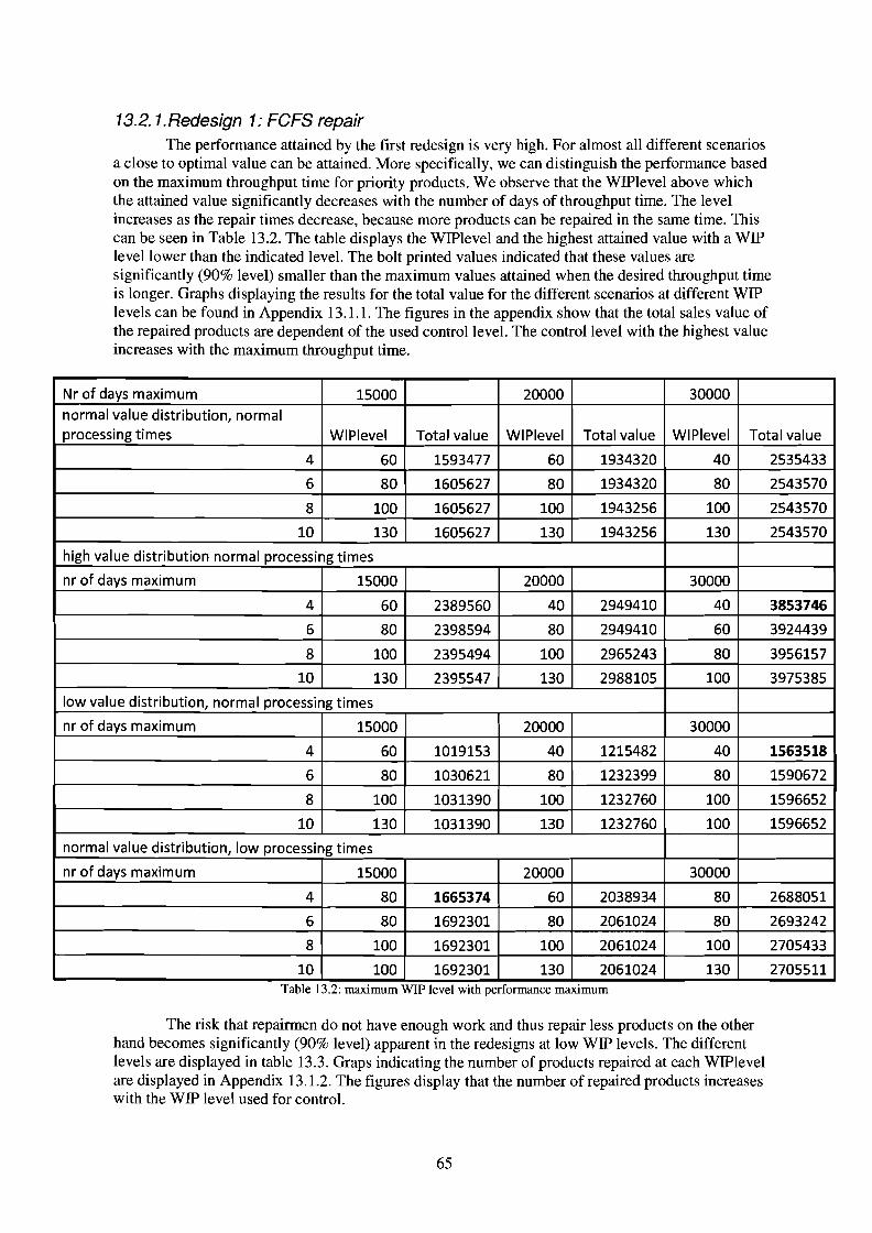
13.2. 1.Redesign 1: FCFS repairThe performance attained by the first redesign is very high. For almost all different scenarios

a close to optimal value can be attained. More specifically, we can distinguish the performance basedon the maximum throughput time for priority products. We observe that the WIPlevel above whichthe attained value significantly decreases with the number of days of throughput time. The levelincreases as the repair times decrease, because more products can be repaired in the same time. Thiscan be seen in Table 13.2. The table displays the WIPlevel and the highest attained value with a WIPlevel lower than the indicated level. The bolt printed values indicated that these values aresignificantly (90% level) smaller than the maximum values attained when the desired throughput timeis longer. Graphs displaying the results for the total value for the different scenarios at different WIPlevels can be found in Appendix 13.1.1. The figures in the appendix show that the total sales value ofthe repaired products are dependent of the used control level. The control level with the highest valueincreases with the maximum throughput time.

Nr of days maximum 15000 20000 30000normal value distribution, normalprocessing times WIPlevel Total value WIPlevel Total value WIPlevel Total value

4 60 1593477 60 1934320 40 2535433

6 80 1605627 80 1934320 80 2543570

8 100 1605627 100 1943256 100 2543570

10 130 1605627 130 1943256 130 2543570

high value distribution normal processing times

nr of days maximum 15000 20000 30000

4 60 2389560 40 2949410 40 3853746

6 80 2398594 80 2949410 60 3924439

8 100 2395494 100 2965243 80 3956157

10 130 2395547 130 2988105 100 3975385

low value distribution, normal processing times

nr of days maximum 15000 20000 30000

4 60 1019153 40 1215482 40 1563518

6 80 1030621 80 1232399 80 1590672

8 100 1031390 100 1232760 100 1596652

10 130 1031390 130 1232760 100 1596652

normal value distribution, low processing times

nr of days maximum 15000 20000 30000

4 80 1665374 60 2038934 80 2688051

6 80 1692301 80 2061024 80 2693242

8 100 1692301 100 2061024 100 2705433

10 100 1692301 130 2061024 130 2705511Table 13.2: maxImum WIP level WIth performance maXImum

The risk that repairmen do not have enough work and thus repair less products on the otherhand becomes significantly (90% level) apparent in the redesigns at low WIP levels. The differentlevels are displayed in table 13.3. Graps indicating the number of products repaired at each WIPlevelare displayed in Appendix 13.1.2. The figures display that the number of repaired products increaseswith the WIP level used for control.

65

Scenario\number of returns: 15000 20000 30000

Normal value distribution, normal processing times 60 40 40

High value distribution, normal processing times 30 40 30

Low value distribution, normal processing times 40 40 40

Normal value distribution, low processing times 60 40 40Table 13.3: WIPlevels from which on the number of repaIrs decreases

Combining the results from the two tables we can construct intervals for the WIP level forwhich the redesign attains its highest value. These are displayed in Table 13.4.

Nr of days maximum 15000 20000 30000

normal value distribution, normal processing WIPlevel WIPlevel WIPleveltimes interval interval interval

4 60 - 60 40 - 60 40 -40

6 60 - 80 40 - 80 40 -80

8 60 -100 40 -100 40 -100

10 60 - >130 40 - >130 40 - >130

high value distribution normal processing times

nr of days maximum 15000 20000 30000

4 30 - 60 40 -40 30 -40

6 30-80 40 - 80 30 - 60

8 30 -100 40 -100 30 - 80

10 30 - >130 40 - >130 30 -100

low value distribution, normal processing times

nr of days maximum 15000 20000 30000

4 40 -60 40-40 40-40

6 40 - 80 40 - 80 40 - 80

8 40 -100 40 -100 40 -100

10 40 - >130 40 - >130 40 -100

normal value distribution, low processing times

nr of days maximum 15000 20000 30000

4 60 -80 40 - 60 40 - 80

6 60 - 80 40 - 80 40 - 80

8 60 -100 40 -100 40 -100

10 60 -100 40 - >130 40 - >130Table 13.4: WIPlevelmtervaIs for the total value of repalfS

The intervals vary in size, with some having the same upper and lower limit. A complicatingfactor is that both the value distribution and the number of returns are unknown beforehand. Then tomake sure the highest possible value of repairs is attained the highest lower limit and lowest upperlimit from the above scenarios needs to be taken. This leads to the aggregate intervals for the differentmaximum throughput times displayed in Table 13.5. Now if the maximum throughput time is fourdays we cannot set a WIPlevel and be confident the maximum attainable value is reached.

66

Maximum throughput time WIPlevel interval

4 60 -40

6 60 - 60

8 60 - 80

10 60 -100Table 13.5. Aggregate WIPlevel Intervals

13.2.2. Redesign 1: Performance of redesign 1 with a priority ruleTo evaluate the perfonnance of the priority rule we will look at the percentage of products

repaired late and within the desired throughput time for all scenarios. If the percentage of productsrepaired late decreases the total value of the repairs increases. Appendix 13.1.3 shows tables for eachscenario indicating the different percentages of products late and within desired time when 70 and90% are priority products. As can be seen the effect of the priority rule varies, the percentage ofproducts repaired late decreases, causing a higher total value of the repairs in all situations whereproducts are repaired late on occasion. The increase in value is dependent on the probability thatproducts are repaired late without the priority rule. The dependency can be seen in Table 13.6, whichis an aggregation of the tables in Appendix 13.1.3. The table displays the average decrease in productsrepaired late caused by the priority rule for different intervals of late products.

Decrease in % late products:

No Priority 1 day 5 days

0-10% 1.1% 1.5%

11-20% 2.7% 4.5%

21-30% 2.1% 4.9%

>30% 1.5% 3.0%Table 13.6: Decrease In late products for 90% pnonty products

We see that the largest increases are observed for the 5 day priority rule. The effect is largestwhen between 11 and 30% of the products are repaired late without priority rule. When the total valueof repairs is already (close) to its highest level without priority, thus when only a small percentage ofproducts are late, the priority rule adds less value and when the probability becomes larger then 30%the effect decreases. The added value is dependent on the value distribution and number of returns peryear.

On the other hand the percentage of products repaired within the desired throughput timevaries from the situation with no priority rule. The effect is shown in Table 13.7.

Decrease in % within the desired throughput time

No priority 1day 5 days

91-100% 0.6% 5.1%

81- 90% 0.6% 0.6%

71-80% 0.2% -1.3%

<70% -0.1% -3.2%Table 13.7. Decrease In products repaIred withIn the desired maxImum for 90% pnonty products

Again we see the effect is stronger when 5 days priority is given. The effect is largest whenmore than 90% of the products are repaired on time, when the redesign without priority is functioningrather well. A positive effect is that when a low percentage «70% for 1 day, <80% for 5 days) of the

67

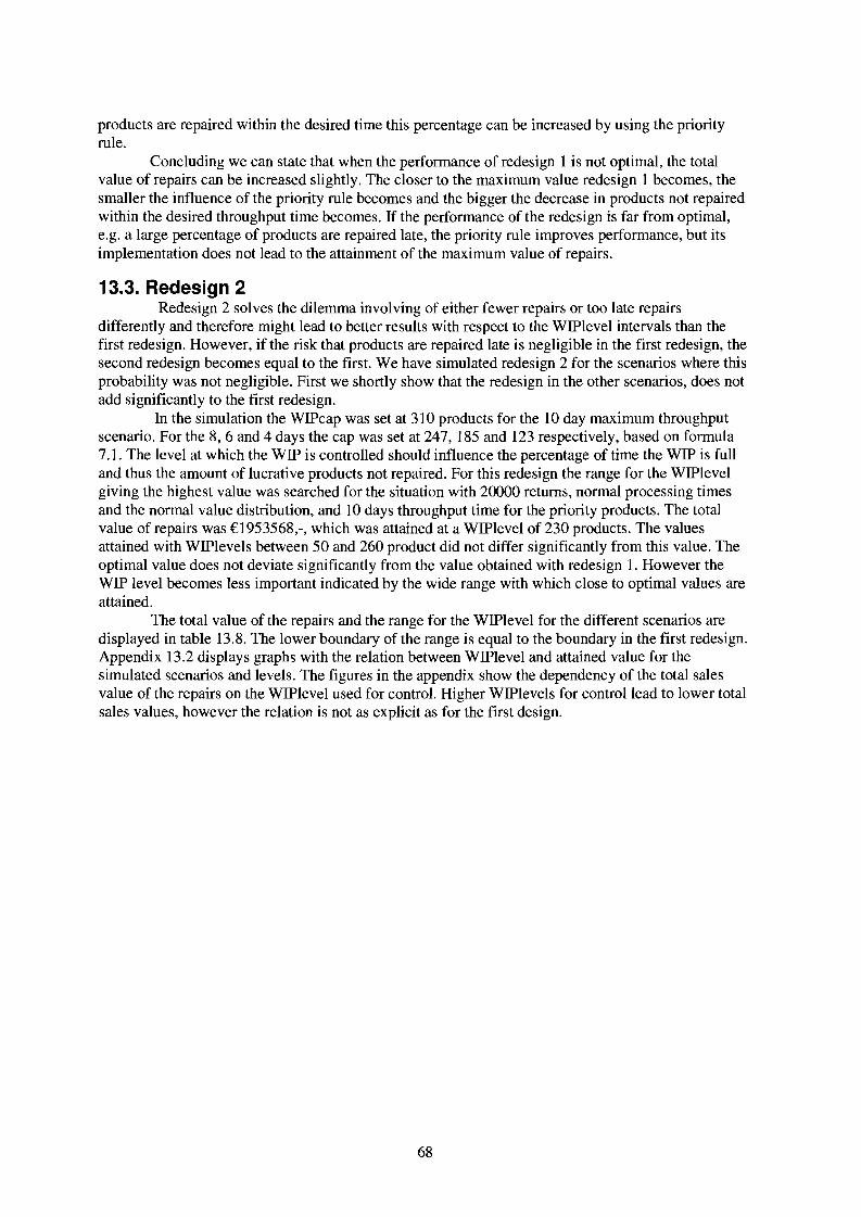
products are repaired within the desired time this percentage can be increased by using the priorityrule.

Concluding we can state that when the performance of redesign 1 is not optimal, the totalvalue of repairs can be increased slightly. The closer to the maximum value redesign I becomes, thesmaller the influence of the priority rule becomes and the bigger the decrease in products not repairedwithin the desired throughput time becomes. If the performance of the redesign is far from optimal,e.g. a large percentage of products are repaired late, the priority rule improves performance, but itsimplementation does not lead to the attainment of the maximum value of repairs.

13.3. Redesign 2Redesign 2 solves the dilemma involving of either fewer repairs or too late repairs

differently and therefore might lead to better results with respect to the WIPlevel intervals than thefirst redesign. However, if the risk that products are repaired late is negligible in the first redesign, thesecond redesign becomes equal to the first. We have simulated redesign 2 for the scenarios where thisprobability was not negligible. First we shortly show that the redesign in the other scenarios, does notadd significantly to the first redesign.

In the simulation the WIPcap was set at 310 products for the 10 day maximum throughputscenario. For the 8, 6 and 4 days the cap was set at 247, 185 and 123 respectively, based on formula7.1. The level at which the WIP is controlled should influence the percentage of time the WIP is fulland thus the amount of lucrative products not repaired. For this redesign the range for the WIPlevelgiving the highest value was searched for the situation with 20000 returns, normal processing timesand the normal value distribution, and 10 days throughput time for the priority products. The totalvalue of repairs was £1953568,-, which was attained at a WIPlevel of 230 products. The valuesattained with WIPlevels between 50 and 260 product did not differ significantly from this value. Theoptimal value does not deviate significantly from the value obtained with redesign 1. However theWIP level becomes less important indicated by the wide range with which close to optimal values areattained.

The total value of the repairs and the range for the WIPlevel for the different scenarios aredisplayed in table 13.8. The lower boundary of the range is equal to the boundary in the first redesign.Appendix 13.2 displays graphs with the relation between WIPlevel and attained value for thesimulated scenarios and levels. The figures in the appendix show the dependency of the total salesvalue of the repairs on the WIPlevel used for control. Higher WIPlevels for control lead to lower totalsales values, however the relation is not as explicit as for the first design.

68

Returns per year: 15000 20000 30000

Nr of days maximum WIPlevel Total value WIPlevel Total value WIPlevel Total value

normal value distribution, normal processing times

4 60 - 80 1592658 40 - 80 1937636 40 - 80 2540334

6 60 - >130 1588940 40 - >130 1947758 40 - >130 2542487

8 60 - >130 1582044 40 - >130 1943189 40 - >130 2548374

high value distribution normal processing times

4 30 - 80 2399574 40 - 80 2953155 30 - 80 3938075

6 30 -100 2404035 40 -100 2955323 30 -100 3954308

8 30 -100 2400719 40 -100 2970646 30 - >130 3921159

10 30 - >130 3939764

low value distribution, normal processing times

4 40 -100 1023202 40 -80 1232386 40 -80 1587945

6 40 - >130 1023745 40 - >130 1228581 40 - >130 1585701

8 40 - >130 1022599 40 - >100 1235332 40 - >130 1584351

10 40->130 1576205

normal value distribution, low processing times

4 60 - 80 1682207 40 - 80 2059737 40 - 80 2690026

6 60 -100 1676008 40 - >130 2049340 40 - >130 2704752

8 60 -100 1642817 40 - >130 2023734 40 - >130 2706194

10 60 - >130 1660148Table 13.8: Total value of repaIrs and WIPlevel mtervals for RedesIgn 2, values m €

The total values of repairs for most scenarios are not significantly lower or higher than for thefirst redesign. The WIPlevel intervals for which they are attained however are wider then for the firstredesign. Also, for the three scenarios in which significant lower values were attained in Redesign 1,this redesign performs significantly better. The upper boundary WIPlevels are above the WIPlevelsfrom below which the number of repairs decreases. Therefore the intervals with unknown arrivals andvalue distribution are all positive in size, as can be seen in table 13.9.

Maximum throughput time WIPlevel interval

4 60 - 80

6 60 -100

8 60 -100

10 60 - >130Table 13.9.: Aggregate WIPlevel intervals for redesIgn 2

13.4. Redesign 3The third redesign reduces the influence of products that are in the WIP too long. Next to that

it makes sure the right products are handled and repaired by an extra level of profitability at therepairmen. However when there is a negligible risk on products being in the WIP too long thisredesign is equal to the first redesign.

Table 13.10 displays the WIPlevel intervals and the attained maximum value for thesimulated scenarios. Again the lower limits are equal to the first redesign. Appendix 13.3 displays thegraphs indicating the relation between WIPlevel and the attained total value. Again the dependency ofthe total sales value on the WIPlevel for control is shown. In the figures the total sales value is largelyindependent from the WIPlevel within the examined range, only for a 4 day maximum throughputtime a significant decrease is observed with a WIPlevel of 130.

69

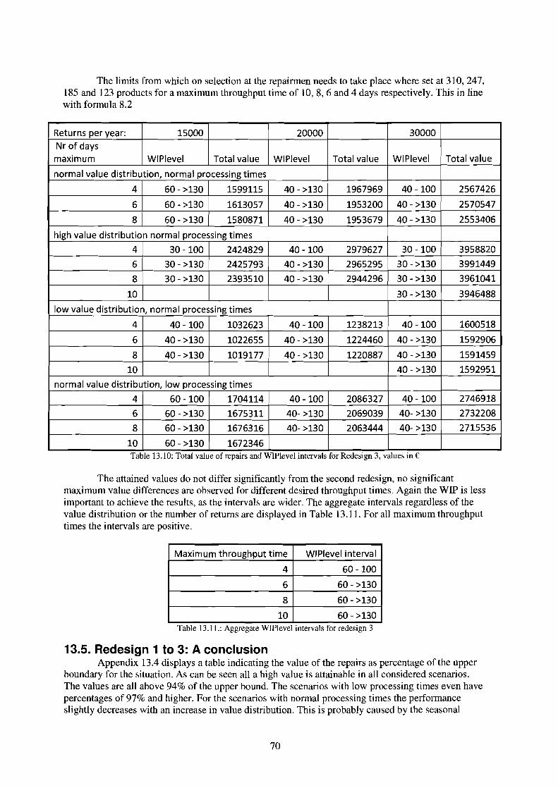
The limits from which on selection at the repairmen needs to take place where set at 310, 247,185 and 123 products for a maximum throughput time of 10, 8,6 and 4 days respectively. This in linewith formula 8.2

Returns per year: 15000 20000 30000Nr of daysmaximum WIPlevel Total value WIPlevel Total value WIPlevel Total value

normal value distribution, normal processing times

4 60 - >130 1599115 40 - >130 1967969 40 -100 2567426

6 60 - >130 1613057 40 - >130 1953200 40 - >130 2570547

8 60 - >130 1580871 40 - >130 1953679 40 - >130 2553406

high value distribution normal processing times

4 30 -100 2424829 40 -100 2979627 30 -100 3958820

6 30 - >130 2425793 40 - >130 2965295 30 - >130 3991449

8 30 - >130 2393510 40 - >130 2944296 30 - >130 3961041

10 30 - >130 3946488

low value distribution, normal processing times

4 40 -100 1032623 40 -100 1238213 40 -100 1600518

6 40 - >130 1022655 40 - >130 1224460 40 - >130 1592906

8 40 - >130 1019177 40 - >130 1220887 40 - >130 1591459

10 40 - >130 1592951

normal value distribution, low processing times

4 60 -100 1704114 40 -100 2086327 40 -100 2746918

6 60 - >130 1675311 40->130 2069039 40->130 2732208

8 60 - >130 1676316 40- >130 2063444 40- >130 2715536

10 60 - >130 1672346Table 13.10: Total value of repaIrs and WIPlevel Intervals for RedesIgn 3, values In €

The attained values do not differ significantly from the second redesign, no significantmaximum value differences are observed for different desired throughput times. Again the WIP is lessimportant to achieve the results, as the intervals are wider. The aggregate intervals regardless of thevalue distribution or the number of returns are displayed in Table 13.11. For all maximum throughputtimes the intervals are positive.

Maximum throughput time WIPlevel interval

4 60 -100

6 60 - >130

8 60 - >130

10 60 - >130Table 13.1 I.: Aggregate WIPlevel Intervals for redesIgn 3

13.5. Redesign 1 to 3: A conclusionAppendix 13.4 displays a table indicating the value of the repairs as percentage of the upper

boundary for the situation. As can be seen all a high value is attainable in all considered scenarios.The values are all above 94% of the upper bound. The scenarios with low processing times even havepercentages of 97% and higher. For the scenarios with normal processing times the performanceslightly decreases with an increase in value distribution. This is probably caused by the seasonal

70

effects and the resulting difference in value of the arrivals which is larger when more expensiveproducts arrive. This seasonality is also the reason that the upper bound is never reached.

The first redesign leads to very good results if the maximum throughput time is 10, 8 and 6days. The risk on useless repair can be controlled whilst the repairmen are not out of work regularly.However, at lower maximum throughput times this is not possible anymore. In these scenarios, whereproducts are repaired late, the priority rule can slightly decrease the probability on this and thusincrease the total value. However the effect of the priority rule is rather small. Besides, the increase intotal value can be accompanied by a decrease in the service for non-priority products. With andwithout priority rule the first redesign there are scenarios in which good results cannot be guaranteedby the first redesign.

The second and third redesigns do perform well in all considered scenarios. On attained valuewe cannot state one is better then the other. The third redesign however is less sensitive to WIPlevels,as can be seen at the wider WIPlevel intervals for this redesign.

When we consider variations outside the scope of the simulation there are differences in theperformance of the redesigns. The performance of the redesigns is now calculated for a given constantcapacity and a given distribution of the arrivals. However in practice it can be that employees get sickcausing less capacity for some days or weeks. On the other hand it can be that due to reasons outsidethe scope of the simulation, e.g. special events like the European Championship soccer, problems atthe delivering logistic service providers, the arrival of products is temporarily very high or very low.These extreme cases are handled differently in the redesigns.

For the first two redesigns sickness leaves can cause late repairs since all products in the WIPneed to be repaired and the temporary decrease in capacity makes sure this takes longer. In Redesign3 when a sickness leave occurs the WIPlevel at the repairmen can be increased to cope with thedecrease in capacity. This leads to more handling and thus slightly fewer repairs, however theserepairs are done on time.

An unexpected temporary large decrease in the arrivals will leave the repairmen out of work.The speed at which they are out of work is dependent on the WIPlevel used for control. The higherthis level is the longer the temporal decrease can be without affecting performance. The WIPcontrollevel can be set highest in Redesign 3, this redesign is therefore more robust against unexpectedtemporal large decreases in arrivals.

A temporary large increase in the number of arrivals on the other hand will in Redesign 1cause the WIP to rise and products to be repaired late. In Redesign 2 this is countered by the WIPcapleading to a better performance, however it is then not sure whether the right products are repaired. InRedesign 3 WIP would rise just as in Redesign 1, but then a raise of the level for repair at therepairmen would prevent products from being late. This would lead to an increase in handling, but themore lucrative products are repaired on time.

We can conclude that Redesign 3 is most robust against the large unexpected changes. Thisredesign also leads to good results in the simulation and therefore is the best of the first threeredesigns.

71

14. Redesign 1 to 3: results for 1 day maximum throughput time

Although, according to RICOLEC, four days is, in practice, the minimal maximumthroughput time for the repair of products, still it is interesting, from an academic point of view, to seehow the different models perform under even shorter maximum processing times. Therefore we haveshortly simulated all three designs for the situation in which the maximum throughput time is only]day. Thus products brought today need to be fixed tomorrow. Here we will first discuss the simulationsettings used, after which the results for the models will be compared.

14.1. Simulation settings &performance evaluationThe WIP control levels were adjusted, compared to the simulation in chapter 13. This because

the repairmen on average only repair 34 products a day, thus control levels higher then 34 can neverlead to high results. The redesigns were therefore simulated with control levels of 10 and 20 products.

In this simulation only the normal situation, with normal processing times and a normal valuedistribution was simulated. The priority rule in redesign 1 was not varied, all products were repairedfirst come first served. The percentage of priority products was also kept constant.

For redesign 2 and 3 the WIPcap and the WIPlimit were set on 30 products by solvingformulas 7.2 and 8.1 for 1 day capacity. The maximum attainable value for each of the redesigns isequal to the maximum value discussed in section 13.]. The performance of the redesigns will beevaluated based on the attained value of the repairs as a percentage of the maximum value.

14.2. Results for redesign 1 to 3Table 14.1 displays the results for the simulation of the different situations. It also displays

the percentage of the maximum attained by the different redesigns. As can be seen the third redesignperforms best in all circumstances. The differences between the first and third redesign are significantin all circumstances except 15000 returns and a control level of 10 products. As can be seensignificantly more products are repaired under redesign 2 and 3 than under redesign 1. Under thesimulated circumstances the WIPcap is reached often causing, in contrast to in redesign 1 no laterepairs and a higher total value of repairs, although only significant at a WIP control level of 20 with15000 and 20000 returns.

Under the third redesign significantly more repairs are completed on time than under the firstredesign and therefore this leads to significantly better results with respect to the total attained valuein all simulated circumstances. This is due to the extra selection decision at the repairmen. The thirdredesigns also attains higher values than the second redesign in all simulated circumstances, howeverthis is only significant at a WIP level of 10 products and for a WIP level of 20 products and 20000returns. The differences in total value attained between 10 and 20 products within one redesign showthat redesign three is less depended on the set WIP level then the other redesigns.

15000 20000 30000returns returns returns

Redesign WIPcontrollevel total value Percentage total value Percentage total value Percentage

1 10 1342752 82.2% 1691534.1 84.5% 2137485.9 81.0%

2 10 1343004.9 82.2% 1706191.4 85.2% 2159200.5 84.5%

3 10 1394856 85.3% 1776198.3 88.7% 2277166.4 86.3%

1 20 1419677.7 86.9% 1755359.1 87.7% 2245174.5 85.1%

2 20 1476369.4 90.3% 1804946.6 90.2% 2268877 86.0%

3 20 1478530.4 90.5% 1819730 90.9% 2288635.7 86.8%

Maximum value: 1634430 100.0% 2001487 100.0% 2637870 100.0%Table 14.1: Results under a maxImum throughput time of 1 day

72

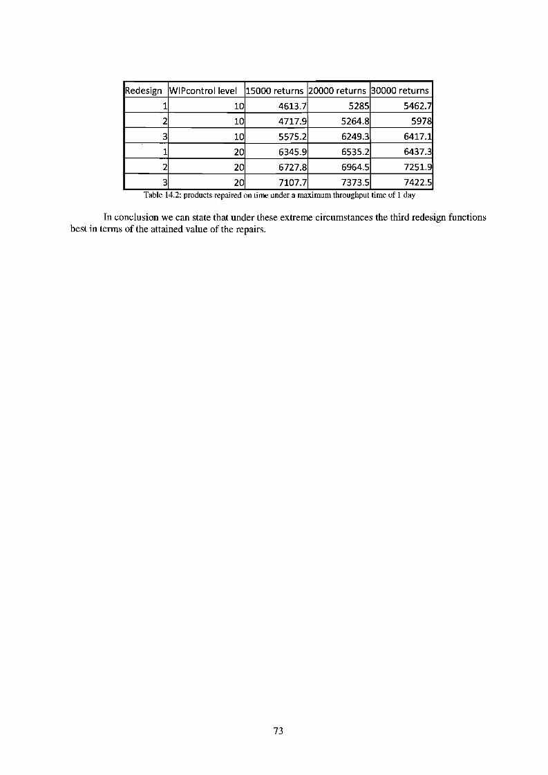
Redesign WIPcontrollevel 15000 returns 20000 returns 30000 retu rns

1 10 4613.7 5285 5462.7

2 10 4717.9 5264.8 5978

3 10 5575.2 6249.3 6417.1

1 20 6345.9 6535.2 6437.3

2 20 6727.8 6964.5 7251.9

3 20 7107.7 7373.5 7422.5Table 14.2: products repaued on time under a maXImum throughput time of 1 day

In conclusion we can state that under these extreme circumstances the third redesign functionsbest in tenus of the attained value of the repairs.

73

15. Decreasing capacity: redesign 3, results

15.1. Capacity: the influence of a decrease in capacityWe have shortly examined the effect of decreasing the capacity available for repair. Only a

decrease is examined since RICOLEC expects not to hire any new personnel when any of the presentrepairmen quits. This for the same reasons as it hires no new personnel on a temporary or fixed basis,being that the time needed to get acquainted with the repair work of the product assortment is verytime consuming and, according to RICOLEC, the labor costs of new workers together with thepossibility that new workers will leave the company quickly do not justify this learning period. Wehave examined three scenarios. All with a maximum throughput time of 4 days and normal processingtimes. This throughput time was chosen because the effect is expected to increase with a decrease inthroughput time since then WIP needs to be controlled on a lower level and 4 days is the lowestpractically possible, according to RICOLEC, throughput time. The effect of a capacity decrease wasmeasured for Redesign 3, since this redesigns leads to the best performance in the simulation. Thecapacity levels considered are 2, 1,5 and 1 fulltime repairmen. The WIPlimits for the redesign werebased on the considered capacity and calculated with formula 8.2. The upper bound on performancewith these capacity levels for the considered scenarios can be found in table 15.1 and was calculatedin the same manner as table 13.1.

Capacity (persons): 1 1.5 2Value distribution Returns per year Value (€) Value (€) Value (€)

normal value distribution 20000 1405006 1699670 1875280

high value distribution 30000 3200263 3560057 3859457

low value distribution 15000 701175 861600 975080Table 15.1.: Upper bounds on the total value of repmrs for dIfferent levels of capacIty

Table 15.2 depicts the maximal attainable value and its percentage of the upper bound percapacity level and simulated circumstances. Graphs displaying the value of repairs per WIPcontrollevel for the different scenarios can be found in Appendix 15. The graphs show that the total value isdependent upon the WIPlevel, a too high WIPlevel for control leads to a lower total value due to a lotof late repairs. A too low WIPlevel for control leads to a lower total value due to the repair of fewerproducts. This relation is most strongly shown in appendix figure 15.9.

Capacity(persons): 1 1.5 2

Value distribution Returns per year Value (€) % Value (€) % Value (€) %

normal value distribution 20000 1254584 89.3% 1560478 91.8% 1774845 94.6%

high value distribution 30000 2974907 93.0% 3369213 94.6% 3681917 95.4%

low value distribution 15000 626446.4 89.3% 803492.8 93.3% 928129.8 95.2%Table 15.2: Performance of RedesIgn 3 under dIfferent capacIty for repaIr

The performance of Redesign 3 goes down with decreasing capacity. This is due to the lowerWIPlevels for control that should be used to prevent excessive handling of repairs by the repairmenwhich carries the inherent risk that the repairmen are out of work as can be seen in the graphs inAppendix 15. However even if only one repairman is available and the maximum throughput time isonly 4 days still at least 89% of the total value can be repaired. It is expected that the percentage willincrease for longer maximum throughput times since then a higher WIPlevel for control can be used.

74

16. Design 4: results

16.1. Redesign 4: expected benefitsDue to the high performance attainable with the first three redesigns it is questionable

whether redesign 4, with individual product access would lead to large further improvements.In the fourth redesign no handling of the batches is needed anymore, but the individual

handling times for the products are unknown. The maximum attainable value of the repairs when nohandling is needed is depicted in table 16.1. In the table only the time needed for out of warrantyrepairs is subtracted from the total capacity.

Scenario/ returns per year 15000 20000 30000

normal value distribution, normal processing times 1647889 2009188 2664333

high value distribution, normal processing times 2531815 3135296 4174500

low value distribution, normal processing times 1047130 1276037 1635093

normal value distribution, low processing times 1712573 2130204 2794204Table 16.1: Upper boundaries for the different scenarios without handlmg by repairmen, values m €

If we compare the values from table 16.1 with the values attainable by redesign 1 to 3 from chapter13, we see it is in the ideal situation possible to increase the total value of repairs.

In practice, zero handling will be very difficult to realize. However even with zero handlingthe maximum will not be reached due to the fluctuations in arrivals in the year, which make itimpossible to always repair the most lucrative products, as was also seen for redesigns 1 to 3. Theneed of handling decreases the attainable benefits of this redesign. We have examined the upperbound on performance for different handling times. These are displayed in Appendix 16. The upperbounds are obtained by calculating the maximum with increases of the total repair time per product.This increase then resembles the handling time per product needed to take the product from stock.Then the most profitable products are considered for repair until the capacity available for one year isfilled. This does not take into account the maximum throughput times, making the calculations similarto the calculations underlying table 13.1.

Now to judge whether improvement can be made by Redesign 4, we subtracted the maximalattained values of Redesign 3, which are at least equally good than those of the other two redesigns.The potential improvement decreases with the handling time and for each scenario there is a handlingtime for which the upper bound on Redesign 4 is equal to the performance of redesign 3. Table 16.2displays this handling time, being 1, 3, 5, 7 or 9 minutes for the different scenarios.

75

Returns per year: 15000 20000 30000

Nr of days maximum minutes minutes minutes

normal value distribution, normal processing times

4 5 3 5

6 5 3 5

8 7 3 7

10 5 5 7

high value distribution normal processing times

4 7 7 5

6 7 7 5

8 9 9 5

10 9 7 5

low value distribution, normal processing times

4 3 5 3

6 3 5 3

8 3 5 3

10 3 5 3

normal value distribution, low processing times

4 1 3 3

6 3 3 3

8 3 3 3

10 3 3 3Table 16.2: Break even handhng Urnes m mmutes for RedesIgn 4

This analysis assumes no seasonal effects are apparent. Therefore in practice the handling times needto be smaller then suggested figures to obtain benefits from redesign 4. Overall an improvement,when the repairmen capacity is 2,5 men, is only likely when the handling time per product can bedecreased compared to the batch scenario. The individual access therefore does not lead to significanthigher performance, but a decrease in handling time can lead to an increase. However this decreasemight also be attained while still handling the products in batches.

The redesign might become appealing when the repair capacity decreases to I or 1,5repairman and the maximum throughput times decreases to 4 days, since then the third redesignperforms less good. The functioning of redesign 4 does not depend on capacity if the products notrepaired are taken out of the WIP and are handled by other employees than the repairmen. Then therepairmen can be kept working and no risk on late repairs is apparent. However this requires extracapacity of other employees.

76

17. ReCOn1mendationsThis report focuses on answering two different research questions as stated in section 2.5. We

will first discuss the recommendations for the first research question. After this the recommendationsfor the second research question will be discussed for each decision.

17.1. Insight in the failure of not repaired productsCurrently RICOLEC does not know what causes the failure on not repaired products.

However, as discussed in chapter 2 this information can be of use. Therefore the following researchquestion was formulated:

How can RICOLEC obtain insight in thefai/ure of its products in the field by testing productsreceived in the warranty return flow?

Now for RICOLEC to attain insight in the failures of product type series a number of returnedproducts need to be tested. In order to achieve considerable precision and confidence the number oftested products per series will be in the order of 20 to 30 products. The testing of the products with thecurrent size and quality of the assortment will probably require less than 300 hours of a tester on ayearly basis. In order to facilitate the testing of the right amount of products the procedure developedin this report can be implemented to obtain fast and relatively detailed insight in the failure behaviorof not repaired products based on IRIS codes. However, the testing procedure prescribes the testing ofthe first arriving returns. This to secure that the results of the tests are available rapidly. However thissample is not random and can therefore lead to biased results. This limits the statistical value of theprocedure. The effect of sampling the first products compared to a random sample could be examined.

Also RICOLEC should look into the use of the results from the tests. In the near futureprocedures should be developed that assist in the timely and adequately use of the results, both withrespect to communication to suppliers and improvements of product support. Also the test procedureresults can be used in the purchase of new product types.

17.2 Processing of warranty returnsRICOLEC at the moment is unsure that it is processing its warranty returns in the right way

and feels that this process can be improved upon, as stated in chapter 2. Therefore the followingresearch question was formulated:

How should the submitted warranty claims and products flow be allocated to the differentsettlement/processing combinations in order to process the claims and products more cost-effectively?

This research question can be subdivided in partial research question each involving one decision inthe process as it shown in figure 5.1. Therefore we will also address the recommendations for eachdecision separately

17.2. 1. Repair or not? what and how much to repairFour different redesigns were constructed. Of the first three redesigns the performance was

determined by simulation. This showed that in the current situation with 10 days throughput time allthree redesigns function equally well and with all redesigns close to optimal performance can beachieved. If the maximum throughput time is lowered to 4 days however, the second and thirdredesigns lead to better results than the first redesign. The performance of the first redesign in thissituation can be improved by including a priority rule. However the improvement does not lead to thesame high results as attained with redesign 2 and 3. Taking into account not simulated variations wehave to conclude that redesign 3 is the most robust redesign and will lead to equal or betterperformance than the first and second redesign in all relevant situations. The performance of thisredesign decreases slightly with a decrease in capacity; however it remains close to or above 90% ofthe upper boundary.

77

The fourth redesign will, with the current capacity, not lead to significant improvementsunless the handling time of products can be reduced to very low levels. Therefore the implementationof this redesign is not recommended. The redesign might become interesting if both the maximumthroughput time and capacity are severely lowered. However, the increase in performance will then belarger in percentage and smaller in value due to the lower maximum values.

We must note that the performance ofthe different redesigns was examined for a seasonalarrival pattern. However both the degree of seasonality and the variation in the arrivals were notvaried since RICOLEC does not expect these variables to change. Still, variation in these variablesmight influence the result.

Concluding we recommend the implementation of the third redesign in view of expectedfuture developments and robustness to unexpected variations. In the implementation the solution canbe refined to better include two variables for which assumptions needed to be made in the simulation.Firstly, the probability of a failing repair was not taken into account in the simulation and in theformula to determine the profitability of repair. The probability that cannibalization was needed wasnot differentiated to product type in both the simulation and the measure of profitability. Both thesevariables can be measured in the newly made information system that also includes the redesign andcan therefore be included in future refinements. Secondly, the repair times for the different productswere not known precisely and had to be estimated based on interviews with the repairmen. Therepairmen have demonstrated willingness to register their repair times and this can be included in thenewly constructed system. The resulting repair times can be used to update and refine the redesign.

For the future RICOLEC can look into two other things that might lead to improvements inthe processing of the returns. First, on a more conceptual basis, RICOLEC could look into thepossibility of like-for-like repair in which it is not necessary to return the exact same (repaired)product, to a customer but just one of the same product type. This would alter the production controlsituation, production to stock could be partially applied possibly limiting the effect of seasonality,however it would probably not make its control easier. Besides this, it is far from guaranteed betterresults could be attained. Secondly RICOLEC can reduce the returns, especially returns with notechnical failures, by better product support via e.g. brand websites and user-manuals.

17.2.2. Cannibalize or not?We conclude that it is not economically attractive for RICOLEC to invest in the optimization

of its stock keeping system to decide upon cannibalization. This due to the diversity in the used parts,the low quantities per part and the relatively low value of the parts together with the largerequirements with respect to needed information to construct an optimal policy to determine whichproducts to cannibalize. A simple policy was developed and to facilitate the decision making thispolicy can be implemented. However, this policy is limited with respect to the control of the stockingfor cannibalization of products and the stock keeping of the products to be cannibalized. In the futureRICOLEC could look into the incorporation of demand for cannibalized parts into the procedure toimprove upon the selection of products, at the moment this was not possible due to a lack of data withrespect to the use of cannibalized parts.

17.3.3. Replace or reimburse?The decision whether to replace a product for a new one or reimburse a submitter needs to

take into account various other considerations than purely financial ones. Besides this the physicalpossibility to replace a product is variable and unknown. Therefore we cannot conclude when whichoption should be chosen. If financial considerations are the sole concern then the proposed decisionstructure can be implemented. However, since non-financial motives are leading in this decision theproposed decision structure is only of little practical use. RICOLEC wishes to fulfill the wishes of theclaim submitter with respect to replacement or reimbursement from the viewpoint of customerservice. However these wishes are not known for all the customers. Therefore it might be interestingto see what the wishes of the submitters are with respect to this decision. Then RICOLEC can base itsdecisions better upon these wishes.

78

18. Conclusion on the contribution to academic literature

18.1. Contribution to the academic literatureWhen the maximum throughput times are large all redesigns can lead to high performance.

The different order acceptance policies do not lead to different results. However when throughputtimes or Due Dates become more stringent the more elaborated order acceptance policies of Redesign2 and Redesign 3 perform better than the simple order acceptance policy of Redesign 1. Translatingthis to Kingsman's (2000) model the control over both input and queue only adds to the performanceof a production system compared to only input control in case of stringent maximum throughputtimes, as is evident from the better performance of redesign 3 under short practical maximumthroughput times and maximum throughput times of 1 day. Stringent maximum throughput times aredefined as throughput times where no WIP level can be chosen that both controls the risk on latedelivery as well as a high occupancy rate.

These findings need to be placed into perspective. In this report the different order acceptancepolicies have been tested under numerous scenarios, however all with seasonality and a fixedvariation. Also the cost function was not varied. The order acceptance policies should be examined fordifferent arrival scenarios and cost functions (e.g. a cost function based on the tardiness of products)in order to generalize the insights.

Still, the conclusion is similar to the conclusions drawn by ten Kate (1994) and Wester et at(1992) that conclude the integration of scheduling and order acceptance only yields better results forstringent Due Dates. Although we do not consider scheduling we do extend the order acceptancefunction to account for the status of the system in more detail.

With respect to the performance of production control mechanisms with a WIPcap insituations with variable rewards it can be concluded that when the WIPcap is close to the WIP levelused for control the average value of repairs decreases because of the refusal to repair lucrativeproducts as was expected by Van Ooijen and Bertrand (2003). This effect decreases with thedifference between the WIPcontrollevel and the WIPcap.

Lastly it was shown that under large maximum throughput times close to optimalperformance can be achieved with batch stock keeping of products. Also when throughput timesbecome more stringent the results attainable with batch stock keeping are high, although only formore complex order acceptance policies. However with stringent throughput times and a smallcapacity it might be that individual product stock keeping and the larger opportunities with respect toscheduling lead to better performance than batch stock keeping. Simulation of the situation in whichproducts are individually accessible is needed to draw definite conclusion in this respect.

79

References

Abdul-Razaq, T.S. Potts, e.N. and Van Wassenhove, L.N. (1990), A survey of algorithms for thesingle machine total weighted tardiness scheduling problem, Discrete Applied Mathematics, 26, 235­253

Van Aken, J.E. Berends, H. and Van der Bij, H. (2007), Problem Solving in Organizations,Cambridge University Press, Cambrigde, United-Kingdom

Bertrand, J.W.M., Wortmann, J.C. and Wijngaard, J. (1988), Production-control and materialmanagement (in Dutch), Wolters-Noordhoff, Groningen, The Netherlands

Brombacher, A.e. (1999), Maturity index on reliability: covering nontechnicalaspects of IEC61508 reliability certification. Reliability Engineering and System Safety, 66, 109-120.

Brombacher, A.e. Sander, P.e. Sonnemans and P.I.M. Rouvroye, J.L. (2005)Managing product reliability in business processes 'under pressure', Reliability Engineering andSystem Safety, 88, 137-146

Chen, ZL Lu, Q. and Tang, G. (1997), Single machine scheduling with discretely controllableprocessing times, Operations Research Letters, 21, 69-76

Cooper, D.R. and Schindler, P.S. (2003), Business research methods, McGraw-Hill, New-York, USA

Dauzere-Peres, S. (1995), Minimizing late jobs in the general one machine scheduling problem,European Journal ofOperational Research, 81, 134-142

Di Bucchianico, A. (2000), Statistisch Compendium, Faculty of Mathematics and computertechnology, Eindhoven University of Technology, Eindhoven, the Netherlands (in Dutch)

Ebben, M.I.R. Hans, E.W. and aIde Weghuis, F.M. (2005), Workload based order acceptance in jobshop environments, OR Spectrum, 27, 107-122

EU (2002), Directive 2002/96IEC of the European parliament and of the council of 27 January 2003on waste electrical and electronic equipment (WEEE) - joint declaration of the European parliament,the council and the commission relating to article 9. Official Journal L037: 24-39

Flapper, S.D.P. (2005), On the value of warranty returns, Working paper, Eindhoven University ofTechnology, Eindhoven, The Netherlands

Framinan, J.M., Gonzalez, P. L. and Ruiz-Usano, R. (2003), The CONWIP production controlsystem: review and research issues, Production Planning & Control, 14,255 - 265

Framinan, J.M., Gonzalez, P.L. and Ruiz-Usano, R. (2006), Dynamic card controlling in a Conwipsystem, International Journal of Production Economics, 99, 102-116

Goossenaerts, J.B.M. and Pels, H.I. (2005). Methodology for the simulation ofoperational processes,Eindhoven University of Technology, Eindhoven, the Netherlands

Hopp, W. J. and Roof, M. L. (1998), Setting WIP levels with statistical throughput control (STC) inCONWIP production lines, International Journal ofProduction Research, 36, 867 - 882

Hopp, W.J. and Spearman, M.L. (2000), Factory Physics International edition, McGraw-Hill, New­York, USA

80

Huang, M., Wang, D. and Ip, W.H. (1998), Simulation study of CONWIP for a cold rolling plant,International Journal ofProduction Economics, 54, 257 - 266

Jack, N. and Murthy, D.N.P. (2001), A servicing strategy for items sold under warranty, Journal ofthe Operational Research Society, 52, 1284-1288

Jack, N. and Van der Duyn Schouten,F. (2000), Optimal repair/replace strategies for a warrantedproduct, International Journal ofProduction Economics, 67, 95-100

Jensen, K. and Rozenberg, G. (eds.) (1991), High level Petri nets: Theory and Application, SpringerVerlag, Berlin, Germany

Ten Kate, H.A. (1994), Towards a better understanding of order acceptance, International Journal ofProduction Economics, 37 , 139-152

Ketzenberg, M.E. Van der Laan, E. and Teunter, RH. (2006), Value of Information in Closed LoopSupply Chains, Production and Operations Management, 15, 393-406

Kennedy, W.J. Patterson, J.W. Fredendall, L.D. (2002), An overview of recent literature on spareparts inventories, International Journal Production Economics, 76, 201-215

Kingsman, B.G. (2000), Modelling input-output workload control for dynamiccapacity planning in production planning systems, International Journal ofProduction Economics,68,73-93

Van der Laan, E. Dekker, R Salomon, M. (1996), Product remanufacturing and disposal: Anumerical comparison of alternative control strategies, International Journal ofProductionEconomics, 45, 489 - 498

Lawler, E.L. (1994), Knapsack-like scheduling problems, the Moore-Hodgson algorithm and the'tower of sets' property, Mathematical Computer Modeling, 20, 91-106

Lee, LS. Sung, C.S. (2008), Minimizing due date related measures for a single machine schedulingproblem with outsourcing allowed, European Journal ofOperational Research, 186, 931-952

Lewis, H.P. and Slotnick S.A. (2002), Multi-period job selection: planning work loads to maximizeprofit, Computers & Operations Research, 29, 1081-1098

Lu, Y., Loh, H.T., Brombacher, A.c., and Den Ouden, E. (2000), Accelerated stress testing in a time­driven product development process, International Journal ofProduction Economics, 67, 17-26

M'Hallah, R. Bulfin, R.L. (2007) , Minimizing the weighted number of tardy jobs on a single machinewith release dates, European Journal ofOperational Research, 176, 727-744

Moore, J.M. (1968), A njob, one machine sequencing algorithm for minimizing the number oflatejobs, Management Science, 15, 102-109

Murthy, D.N.P. (1996), Chapter 24: Warranty Servicing, in: Product Warranty Handbook, Blischke,W.R. and Murthy, D.N.P. (eds.), Marcel Dekker, New York, USA

Murthy, D.N.P., and Blischke, W.R (2005), Warranty management and product manufacture,Springer-Verlag, London, United-Kingdom

81

Murthy, D.N.P., Solem, 0., and Roren, T. (2004), Product warranty logistics: Issues and challenges,European Journal ofOperational Research, 156, 110-126

Van Ooijen, H.P.G. and Bertrand, J.W.M. (2003), The impact of arrival rate control on the economicperformance of make-to-order firms with Work In Process (in)dependent order processing rates,Working paper, Eindhoven University of Technology, Eindhoven, the Netherlands

Petkova, V. (2003), An analysis of field feedback in consumer electronics industry, PhD thesis,Technical University Eindhoven, Eindhoven, The Netherlands

Potts, C.N. and Van Wassenhove, L.N. (1998), Algorithms for scheduling a single machine tominimize the weighted number of late jobs, Management Science, 34, 843-858

Roderick, L.M. Toland, J. and Rodriguez, F.P. (1994), A simulation study of CONWIP versus MRPat Westinghouse, Computers and Engineering, 26,237-242

Sevaux, M. and Dauzere-Peres, S. (2003) Genetic algorithms to minimize the weighted number of latejobs on a single machine, European Journal ofOperational Research, 151,296 - 306

Rom, W.O. and Slotnick, S.A. (2008) Order acceptance using genetic algorithms, Computers andOperations research, In Press

Silver, E.A., Pyke, D.F., and Peterson, R. (1998), Inventory Management and Production Planningand Scheduling, John Wiley and Sons, New York, United States

Thierry, M. Salomon, M., Van Nunen, J., and Van Wassenhove, L. (1995), Strategic issues in productrecovery management, California Management Review, 37, 114-136.

Wang, K.S. Hsu, F.S. and Liu, P.P. (2002), modeling the bathtub shape hazard rate function in termsof reliability, Reliability Engineering and Systems Safety, 75,397-406

Widmer, R. Oswald-Krapf, H. Sinha-Khetriwal, D. Schnellmann, M. Boni, H. (2005), GlobalPerspectives on E-waste, Environmental Impact Assessment Review 25, 436--458

Yang, B. Geunes, J. and O'Brien, W.J. (2004), A heuristic approach for minimizing weightedtardiness and overtime costs in single resource scheduling, Computers & Operations Research, 31,1273-1301

Zijm, W.H.M. (2000), Towards intelligent manufacturing planning and control systems, ORSpectrum, 22, 313-345

Presentations:

How IRIS Works, presentation of the EICTA

IRIS_course, presentation of the EICTA

82

Appendix

Table of contentsTable of contents 83

Appendix 3 84

Appendix 3.1: Search method & terms 84

Appendix 3.2: Example part of IRIS-code table as used by RICOLEC 85

Appendix 4 86

Appendix 4.1 Returnstream magnitude and division during the years 2005-2007 86

Appendix 4.2: Returns division returns in product groups in 2006 91

Appendix 4.3: Number of repaired warranty returns 109

Appendix 4.4: The failure behavior of to be repaired warranty returns 109

Appendix 12 124

Appendix 12.1. Design 1 125

Appendix 12.2: Design 2 129

Appendix 12.3: Design 3 131

Appendix 12.4: Declarations 137

Appendix 13 139

Appendix 13.1: Results for Design 1 139

Appendix 13.2. Results for Design 2 161

Appendix 13.3. Results for Design 3 167

Appendix 13.4: Result for design 1-3 174

Appendix 15: Results for varying capacity for design 3 175

Appendix 15.1: normal value distribution, normal processing times 175

Appendix 15.2: high value distribution, normal processing times 176

Appendix 15.3: low value distribution, normal processing times 178

Appendix 16: Results for Design 4 180

Appendix 16.1: Upper bounds for varying handling times 180

83

Appendix 3

Appendix 3.1 : Search method & termsTable 3.1 displays the terms used in searches for relevant literature with respect to production

control, order acceptance and scheduling. The searches were conducted using the Abi-Inform andScience Direct databases as indicated in the table. The terms were searched for in the citation, abstractand keywords. The reliance of an article was firstly judged on article title and secondly on abstract.Besides this potentially relevant articles cited in the found articles were explicitly searched for usingAbi-Inform, Science Direct, Jstor, Springerlink and Taylor and Francis databases.

Abi·Infonn: Science direct:Repair, Refund Repair, Refund

Repair, throughput time Repair, reimbursement

Repair, planning, replacement Repair, throughput time

Repair, reverse logistics Repair, planning, replacement

Repair, value-of-time Repair, scheduling

Remanufacturing, value-of-time Repair, reverse logistics

Remanufacturing, value-of-information Repair, value-of-time

Repair, value-of-time One machine scheduling, linear programming

Repair, value-of-information, " Order acceptance, scheduling

Remanufacture, value-of-information Order acceptance, 2-stage

Remanufacture, value-of-time Preliminary, order acceptance

Repair-planning Selection, order-acceptance

Reverse logistics, replace Make-to-order, order-acceptance

Reverse logistics, replacement Order acceptance, throughput time

Repair, warranty Job selection, throughput time

One machine scheduling, linear programming Job selection, sequencing

Reverse logistics, conwip Arrival rate control

Supply uncertainty, conwip Conwip

Make-to-order, conwip Workload regulation

Supply, conwip Order acceptance, Due date

Over supply, conwip WIP, tardiness

Single machine, conwip Late jobs, one machine

Work in process AND Production planning Order acceptance, late products

Batch, sequencing Order acceptance, outsourcing

Workload regulation Scheduling, outsourcing

Order selection Production planning, order acceptance

Scheduling, outsourcing Queue, termination control

Production planning, outsourcing

Production planning, order acceptanceTable 3.1: Search terms per Database

84

• _TIIM!IiUOf--221 Z~,tUQmvWBB

222 Z~FMQmvWGer

2~ lYMKHEKtR1l;GW~li224 Z~~ armt'otmer2m Z~_c:MVAlUiil

22fi Z~.~li'22l' Z~O$~T22fi ZWMOiElI7IN~Sf'2m z~~r~am'f'WBer

D\ ~~TV.wt&IrU~~

W;CJi1iI~armt'AlUiiT~~~

'il'9BfI:RJ.~flHM

~,tUQmvWGS

~FMQmvWBer

lEBtI Kail1E13(I"F~TlEBtI 'IliIFQDtWGSflEBtIliM= ONlVAlUiililEBtI B3ONlVAlUii1tlEBtICS.~1t

~~TVOmvWBS~9lI ~t(RQmvWBer

~Ql\lVotmS'iMagTAl,..E~

~Nf'FJ4i!CICDOIm'.er~ KESfOOlll D~ 1IDa;N f1'ELEFOOIII ffAOCVl_f!Cfi) BIIDCBl:tliaEFOOIII MVOJIDTIftTY GB

C<lJRER~~f

NE~.WJMiiEFMI,.T

~Fli'OB...EEMEli~TCF'iIiP.BI01jJ

Ie part of IRIS-code table as used by RICOLEC

1ft 1XE1 NE'IB1t2 IXElMEl8OP~QFD

1t3 1XElMEl80"~1tt4i IXf;T~Na ~T1U.I~1t15 D:E.rtilE1Bap'~

1tS IXElI'E.O'~O~1t:J' 'Ii8J{T m::BT&T()!'itE1t8 ~TI'i~l\tl1IEI ~TI'i~TlI\I'tNllR'l;;lNDW

1:1~ UB'fl:'.EDrGW~1::::::I::::::I 11B IINWIte,IlI(~aNtCFF

11C ~~ZE}U,ffi9ll13UMI):)m

11D IJlET~T'IlM:EJ,J.

I.........•...·..••.••.:; i.!I\.·~.=EMl.·..~unr~N3; a::w.KB.MJ!~MN

11f~ ~aAnur41'il;T~': 11K ...~TSfolRnIB~

tilt ~ FliQUEMET'l"ClDM

Figure 3.1: part ofIRIScode table as used by RICOLEC (in Dutch)

85

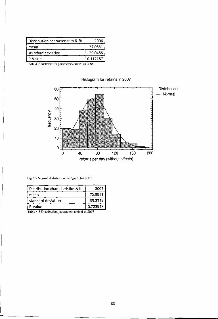
Distribution characteristics & fit 2006

mean 77.0531

standard deviation 29.0488

P-Value 0.112187Table 4.2 DlstnbutlOll parameters amval In 2006

Histogram for returns in 2007

60 Distribution- Normal

50

40>.0c0> 30::J0-0>~- 20

10

00 40 80 120 160 200

returns per day (without effects)

Fig 4.5 Normal distribution histogram for 2007

Distribution characteristics &fit 2007

mean 72.5991

standard deviation 35.3225

P-Value 0.723948Table 4.3 DlstnbutlOn parameters amvalm 2007

88

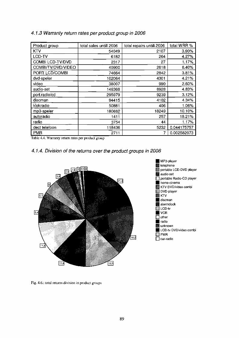
4. 1.3 Warranty return rates per product group in 2006

Product group total sales untill 2006 total repairs untill 2006 total WRR %KTV 54049 2107 3.90%LCD-TV 6182 264 4.27%COMBI LCD-TV/DVD 2317 27 1.17%COMBlfTV/DVDIVIDEO 40900 2618 6.40%PORT.LCD/COMBI 74664 2842 3.81%dvd-speler 102064 4301 4.21%video 38007 990 2.60%audio-set 146368 6928 4.83%port. radio/cd 295979 9239 3.12%discman 94415 4102 4.34%klokradio 50881 406 1.06%mp3-speler 180662 18249 10.10%autoradio 1411 257 18.21%radio 3754 44 1.17%dect telefoon 118436 5232 0.044175757PMR 2711 7 0.002582073

Table 4.4. Warranty return rates per product group

4. 1.4. Division of the returns over the product groups in 2006

• MP3-player• telephoneII portable LCD-DVD player

• audio-setII portable Radio-CD player

• home-cinemaII KTV DVDlvideo combiII DVD-player.KTV.discmanII alarmciockII LCD-tv.VCRII other

• radio• unknown• LCD-tv DVD/video combiIIPMRII car-radio

Fig. 4.6.: total returns division in product groups

89

4. 1.5. Time between purchase and failure

Histogram period after sale

o 100 200 300 400

Period after sale (days)500

Distribution- Exponential

Fig. 4.7. Period between purchase and warranty claim for 1 year warranty products

Histogram for period after sale

800

1)-c:~ 400

I

o 0.2 0.4 0.6 0.8

Period after sale (days)

Distribution- Exponential

1(X 1000.0)

Fig. 4.8 a histogram for the period between purchase and claim filing for 2 year warranty products

90

Appendix 4.2: Returns division returns in product groups in 2006

4.2. 1. Returns not related to warranty claims in 2006

• home-cinema• KTV DVD/video combi~ MP3-player

• portable LCD-DVD playero audio-set.KTV

• telephoneIII DVD-player

• portable Radio-CD player.discman

• unknownOVCR

• LCD-tvIII LCD-tv DVD/video combi

• alarmclock• car-radio

Figure 4.9: division in product groups of returns out of warranty

91

4.2.2. Warranty returns per productgroup in 2006

III MP3-playerIII telephoneI1J portable LCD-DVD playerIII portable Radio-CD playerEJ audio-setIII DVD-playerIII KTV DVDlvideo combiI1J home-cinemaIIIKTVIIIdiscmanIII alarmclockIIlI LCD-tvIII VCREJ otherIII radioIII LCD-tv DVD/video combiIII unknownI1J PMR

Fig. 4.10. Division of the warranty returns in product groups

4.2.3. Division in product groups of not repaired warranty returns in 2006

• MP3-player11IIII telephoneIII portable Radio-CD player• audio-seto DVD-player.discman

• alarmclockI!iiiI portable LCD-DVD playerIII K1V DVDlvideo combi

IIIKTViii home-cinemaiii radio

• earphoneOVCR

• portable speakersiii unknown

• LCD-tvIII walkmano LCD-tv DVD/video combi.PMRIII speaker holders

• adapter

Figure 4.11: division of not-repaired warranty products

92

4.2.4. Percentage of products covered under warranty repaired per product group &product type in 2006

The tables show the number and percentage of product groups/types processed by the repairdepartment and not processed by the repair department thus solely by the collection department.

These tables relate to the tables in Appendix 4.4. in that here the percentage of repairedproducts is shown. Appendix 4.4. then shows the failures, by means of IRrScode classification, of theproducts that were processed by the repair department.

Repair department Total

Productgroup Yes NoProductgr Alarmclock Count 1 389 390oup % within

productgroup ,3% 99,7% 100,0%

audio-set Count 1685 681 2366% withinproductgroup 71,2% 28,8% 100,0%

Discman Count 34 430 464% withinproductgroup 7,3% 92,7% 100,0%

DVD-player Count 445 548 993% withinproductgroup 44,8% 55,2% 100,0%

home-cinema Count 827 67 894% withinproductgroup 92,5% 7,5% 100,0%

KTV Count 615 99 714% withinproductgroup 86,1% 13,9% 100,0%

KTV DVD/video combi Count 777 166 943% withinproductgroup 82,4% 17,6% 100,0%

LCD-tv Count 176 15 191% withinproductgroup 92,1% 7,9% 100,0%

LCD-tv DVD/video combi Count 16 11 27% withinproductgroup 59,3% 40,7% 100,0%

MP3-player Count 379 3970 4349% withinproductgroup 8,7% 91,3% 100,0%

Other Count 1 93 94% withinproductgroup 1,1% 98,9% 100,0%

PMR Count 0 5 5% withinproductgroup ,0% 100,0% 100,0%

portable LCD-DVD player Count 2262 222 2484% withinproductgroup 91,1% 8,9% 100,0%

portable Radio-CD player Count 252 2134 2386% withinproductgroup 10,6% 89,4% 100,0%

Radio Count 4 65 69

93

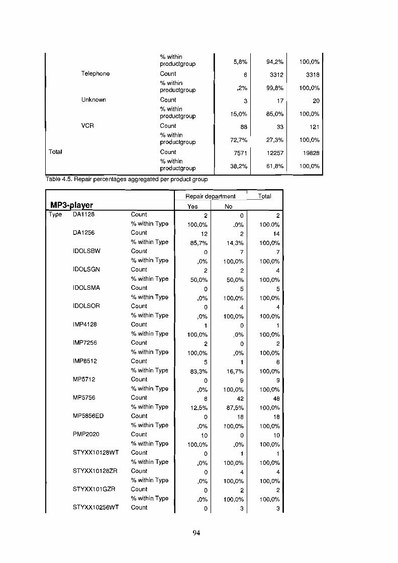
% within94,2% 100,0%productgroup 5,8%

Telephone Count 6 3312 3318% within

99,8% 100,0%productgroup ,2%

Unknown Count 3 17 20% within

85,0% 100,0%productgroup 15,0%

VCR Count 88 33 121% within

27,3% 100,0%productgroup 72,7%

Total Count 7571 12257 19828% within

61,8% 100,0%productgroup 38,2%

Table 4.5. Repair percentages aggregated per product group

Repair department Total

MP3-player Yes NoType DA1128 Count 2 0 2

% within Type 100,0% ,0% 100,0%DA1256 Count 12 2 14

% within Type 85,7% 14,3% 100,0%IDOLSBW Count 0 7 7

% within Type ,0% 100,0% 100,0%IDOLSGN Count 2 2 4

% within Type 50,0% 50,0% 100,0%IDOLSMA Count 0 5 5

% within Type ,0% 100,0% 100,0%IDOLSOR Count 0 4 4

% within Type ,0% 100,0% 100,0%IMP4128 Count 1 0 1

% within Type 100,0% ,0% 100,0%IMP7256 Count 2 0 2

% within Type 100,0% ,0% 100,0%IMP8512 Count 5 1 6

% within Type 83,3% 16,7% 100,0%MP5712 Count 0 9 9

% within Type ,0% 100,0% 100,0%MP5756 Count 6 42 48

% within Type 12,5% 87,5% 100,0%MP5856ED Count 0 18 18

% within Type ,0% 100,0% 100,0%PMP2020 Count 10 0 10

% within Type 100,0% ,0% 100,0%STYXX10128WT Count 0 1 1

% within Type ,0% 100,0% 100,0%STYXX10128ZR Count 0 4 4

% within Type ,0% 100,0% 100,0%STYXX1 01 GZR Count 0 2 2

% within Type ,0% 100,0% 100,0%STYXX10256WT Count 0 3 3

94

% within Type ,0% 100,0% 100,0%STYXX10256ZR Count 2 15 17

% within Type 11,8% 88,2% 100,0%STYXX10512 Count 3 7 10

% within Type 30,0% 70,0% 100,0%STYXX111GR Count ° 1 1

% within Type ,0% 100,0% 100,0%STYXX11256RWT Count ° 8 8

% within Type ,0% 100,0% 100,0%STYXX11512R Count 3 7 10

% within Type 30,0% 70,0% 100,0%STYXX12256ZT Count ° 2 2

% within Type ,0% 100,0% 100,0%STYXX12512ZT Count ° 1 1

% within Type ,0% 100,0% 100,0%STYXX15128ZW Count ° 1 1

% within Type ,0% 100,0% 100,0%STYXX16256WT Count ° 2 2

% within Type ,0% 100,0% 100,0%STYXX16512WT Count 1 9 10

% within Type 10,0% 90,0% 100,0%STYXX25512GN Count ° 3 3

% within Type ,0% 100,0% 100,0%STYXX25512RGN Count ° 3 3

% within Type ,0% 100,0% 100,0%STYXX25512RZT Count ° 3 3

% within Type ,0% 100,0% 100,0%STYXX30128ZR Count 10 1 11

% within Type 90,9% 9,1% 100,0%Total Count 59 163 222

% within Type 26,6% 73,4% 100,0%

Table 4.6.: repaIr percentage for MP3-players.

Repair department Total

Telephone Yes NoType 6131 Count ° 64 64

% within Type ,0% 100,0% 100,0%6132 Count ° 2 2

% within Type ,0% 100,0% 100,0%6141 Count ° 59 59

% within Type ,0% 100,0% 100,0%6142 Count ° 37 37

% within Type ,0% 100,0% 100,0%ME40501 Count 2 77 79

% within Type 2,5% 97,5% 100,0%ME40504 Count ° 1 1

% within Type ,0% 100,0% 100,0%ME40511 Count ° 37 37

% within Type ,0% 100,0% 100,0%ME40512 Count 1 70 71

% within Type 1,4% 98,6% 100,0%

95

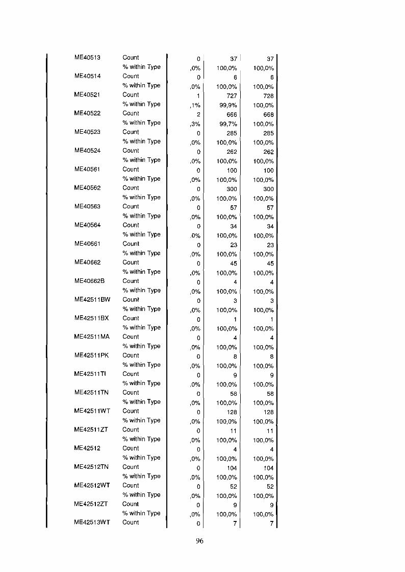
ME40513 Count ° 371 37% within Type ,0% 100,0% 100,0%

ME40514 Count ° 6 6% within Type ,0% 100,0% 100,0%

ME40521 Count 727 728% within Type ,1% 99,9% 100,0%

ME40522 Count 2 666 668% within Type ,3% 99,7% 100,0%

ME40523 Count ° 285 285% within Type ,0% 100,0% 100,0%

ME40524 Count ° 262 262% within Type ,0% 100,0% 100,0%

ME40561 Count ° 100 100% within Type ,0% 100,0% 100,0%

ME40562 Count ° 300 300% within Type ,0% 100,0% 100,0%

ME40563 Count ° 57 57% within Type ,0% 100,0% 100,0%

ME40564 Count ° 34 34% within Type ,0% 100,0% 100,0%

ME40661 Count ° 23 23% within Type ,0% 100,0% 100,0%

ME40662 Count ° 45 45% within Type ,0% 100,0% 100,0%

ME406628 Count ° 4 4% within Type ,0% 100,0% 100,0%

ME425118W Count ° 3 3% within Type ,0% 100,0% 100,0%

ME425118X Count ° 1 1% within Type ,0% 100,0% 100,0%

ME42511 MA Count ° 4 4% within Type ,0% 100,0% 100,0%

ME42511 PK Count ° 8 8% within Type ,0% 100,0% 100,0%

ME42511T1 Count ° 9 9% within Type ,0% 100,0% 100,0%

ME42511TN Count ° 58 58% within Type ,0% 100,0% 100,0%

ME42511WT Count ° 128 128% within Type ,0% 100,0% 100,0%

ME42511ZT Count ° 11 11% within Type ,0% 100,0% 100,0%

ME42512 Count ° 4 4% within Type ,0% 100,0% 100,0%

ME42512TN Count ° 104 104% within Type ,0% 100,0% 100,0%

ME42512WT Count ° 52 52% within Type ,0% 100,0% 100,0%

ME42512ZT Count ° 9 9% within Type ,0% 100,0% 100,0%

ME42513WT Count ° 7 7

96

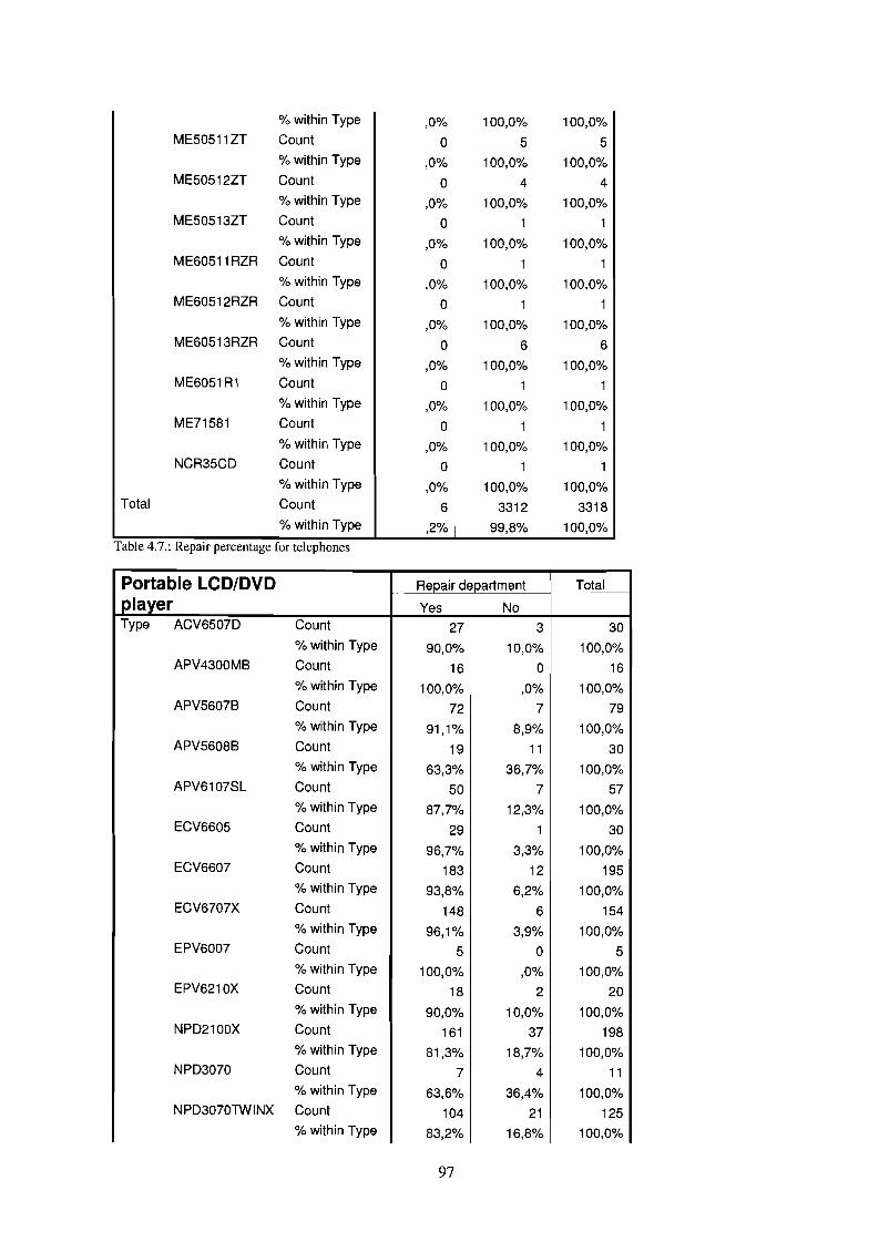
% within Type ,0% 100,0% 100,0%ME50511ZT Count ° 5 5

% within Type ,0% 100,0% 100,0%ME50512ZT Count ° 4 4

% within Type ,0% 100,0% 100,0%ME50513ZT Count ° 1 1

% within Type ,0% 100,0% 100,0%ME60511 RZR Count ° 1 1

% within Type ,0% 100,0% 100,0%ME60512RZR Count ° 1 1

% within Type ,0% 100,0% 100,0%ME60513RZR Count ° 6 6

% within Type ,0% 100,0% 100,0%ME6051 R1 Count ° 1 1

% within Type ,0% 100,0% 100,0%ME71581 Count ° 1 1

% within Type ,0% 100,0% 100,0%NCR35CD Count ° 1 1

% within Type ,0% 100,0% 100,0%Total Count 6 3312 3318

% within Type ,2% 99,8% 100,0%

Table 4.7.: Repalf percentage for telephones

Portable LCD/DVD Repair department Total

plaxer Yes NoType ACV6507D Count 27 3 30

% within Type 90,0% 10,0% 100,0%APV4300MB Count 16 ° 16

% within Type 100,0% ,0% 100,0%APV5607B Count 72 7 79

% within Type 91,1% 8,9% 100,0%APV5608B Count 19 11 30

% within Type 63,3% 36,7% 100,0%APV6107SL Count 50 7 57

% within Type 87,7% 12,3% 100,0%ECV6605 Count 29 1 30

% within Type 96,7% 3,3% 100,0%ECV6607 Count 183 12 195

% within Type 93,8% 6,2% 100,0%ECV6707X Count 148 6 154

% within Type 96,1% 3,9% 100,0%EPV6007 Count 5 ° 5

% within Type 100,0% ,0% 100,0%EPV621OX Count 18 2 20

% within Type 90,0% 10,0% 100,0%NPD2100X Count 161 37 198

% within Type 81,3% 18,7% 100,0%NPD3070 Count 7 4 11

% within Type 63,6% 36,4% 100,0%NPD3070lWINX Count 104 21 125

% within Type 83,2% 16,8% 100,0%

97

NPD4070X Count 155 27 182% within Type 85,2% 14,8% 100,0%

PVS1080 Count 17 6 23% within Type 73,9% 26,1% 100,0%

PVS123 Count 48 2 50% within Type 96,0% 4,0% 100,0%

PVS12621 Count 42 7 49% within Type 85,7% 14,3% 100,0%

PVS1370 Count 166 13 179% within Type 92,7% 7,3% 100,0%

PVS162W Count 25 0 25% within Type 100,0% ,0% 100,0%

PVS1950 Count 210 17 227% within Type 92,5% 7,5% 100,0%

PVS1950NA Count 139 7 146% within Type 95,2% 4,8% 100,0%

PVS1960 Count 11 0 11% within Type 100,0% ,00

/0 100,0%PVS1970 Count 83 4 87

% within Type 95,4% 4,6% 100,0%PVS1971 Count 368 13 381

% within Type 96,6% 3,4% 100,0%PVS6970 Count 159 15 174

% within Type 91,4% 8,6% 100,0%Total Count 2262 222 2484

% within Type 91,1% 8,9% 100,0%

Table 4.8.: Repair percentage for portable LCD players

Repair department TotalPortable Radio-CDplayer Yes NoType AJ4140 Count 0 281 281

% within Type ,0% 100,0% 100,0%AJC2500 Count 15 14 29

% within Type 51,7% 48,3% 100,0%AJC3200 Count 1 3 4

% within Type 25,0% 75,0% 100,0%AJC3200ZT Count 2 0 2

% within Type 100,0% ,0% 100,0%AJC3250 Count 5 63 68

% within Type 7,4% 92,6% 100,0%AJC3300 Count 7 21 28

% within Type 25,0% 75,0% 100,0%AJC3505 Count 89 103 192

% within Type 46,4% 53,6% 100,0%AJC6041W Count 55 63 118

% within Type 46,6% 53,4% 100,0%AJC6041WWMA Count 5 19 24

% within Type 20,8% 79,2% 100,0%

98

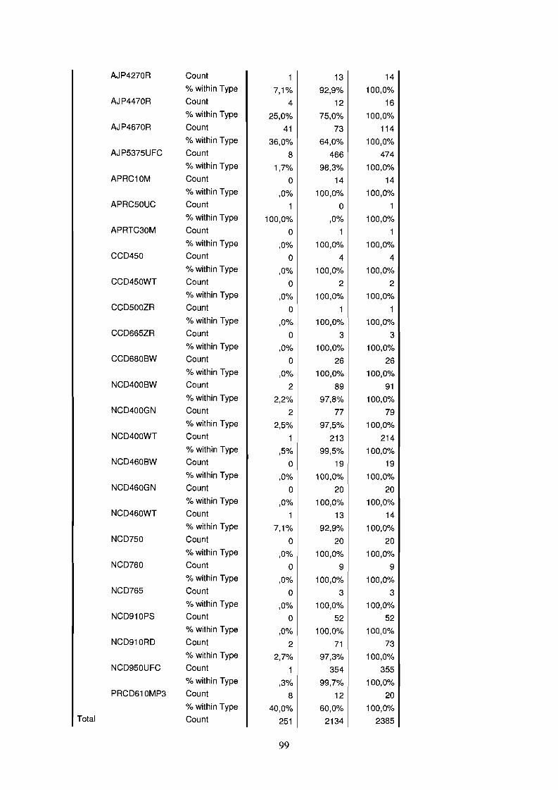
AJP4270R Count 13 14% within Type 7,1% 92,9% 100,0%

AJP4470R Count 4 12 16% within Type 25,0% 75,0% 100,0%

A.IP4670R Count 41 73 114% within Type 36,0% 64,0% 100,0%

AJP5375UFC Count 8 466 474% within Type 1,7% 98,3% 100,0%

APRC10M Count ° 14 14% within Type ,0% 100,0% 100,0%

APRC50UC Count °% within Type 100,0% ,0% 100,0%APRTC30M Count ° 1

% within Type ,0% 100,0% 100,0%CCD450 Count ° 4 4

% within Type ,0% 100,0% 100,0%CCD450WT Count ° 2 2

% within Type ,0% 100,0% 100,0%CCD500ZR Count ° 1

% within Type ,0% 100,0% 100,0%CCD665ZR Count ° 3 3

% within Type ,0% 100,0% 100,0%CCD680BW Count ° 26 26

% within Type ,0% 100,0% 100,0%NCD400BW Count 2 89 91

% within Type 2,2% 97,8% 100,0%NCD400GN Count 2 77 79

% within Type 2,5% 97,5% 100,0%NCD400WT Count 213 214

% within Type ,5% 99,5% 100,0%NCD460BW Count ° 19 19

% within Type ,0% 100,0% 100,0%NCD460GN Count ° 20 20

% within Type ,0% 100,0% 100,0%NCD460WT Count 13 14

% within Type 7,1% 92,9% 100,0%NCD750 Count ° 20 20

% within Type ,0% 100,0% 100,0%NCD760 Count ° 9 9

% within Type ,0% 100,0% 100,0%NCD765 Count ° 3 3

% within Type ,0% 100,0% 100,0%NCD910PS Count ° 52 52

% within Type ,0% 100,0% 100,0%NCD910RD Count 2 71 73

% within Type 2,7% 97,3% 100,0%NCD950UFC Count 354 355

% within Type ,3% 99,7% 100,0%PRCD610MP3 Count 8 12 20

% within Type 40,0% 60,0% 100,0%Total Count 251 2134 2385

99

% within Type 10,5% I

Table 4.9.: Repair percentage for portable radio-CD players

Repair department Total

Audio set Yes NoType AAV2080 Count 2 ° 2

% within Type 100,0% ,0% 100,0%AAV4720 Count 6 ° 6

% within Type 100,0% ,0% 100,0%AMP100 Count 1 ° 1

% within Type 100,0% ,0% 100,0%CDP280 Count 4 2 6

% within Type 66,7% 33,3% 100,0%CMA101 Count ° 1 1

% within Type ,0% 100,0% 100,0%CMA105 Count 2 4 6

% within Type 33,3% 66,7% 100,0%CMA110 Count 1 1 2

% within Type 50,0% 50,0% 100,0%EMRM003 Count 4 12 16

% within Type 25,0% 75,0% 100,0%EMRM015 Count 10 31 41

% within Type 24,4% 75,6% 100,0%ES2 Count ° 1 1

% within Type ,0% 100,0% 100,0%ES3 Count ° 44 44

% within Type ,0% 100,0% 100,0%MICR01500DSSW Count 16 5 21

% within Type 76,2% 23,8% 100,0%MICR0820CD Count 20 1 21

% within Type 95,2% 4,8% 100,0%MICR0820V Count 136 11 147

% within Type 92,5% 7,5% 100,0%MICR0830MP3 Count 83 12 95

% within Type 87,4% 12,6% 100,0%MICR0850D Count 14 1 15

% within Type 93,3% 6,7% 100,0%NASS130 Count ° 1 1

% within Type ,0% 100,0% 100,0%NMA150 Count 1 1 2

% within Type 50,0% 50,0% 100,0%NMA200 Count ° 21 21

% within Type ,0% 100,0% 100,0%NMA250 Count 1 18 19

% within Type 5,3% 94,7% 100,0%NMA301 Count 37 65 102

% within Type 36,3% 63,7% 100,0%NMA321 Count 3 4 7

% within Type 42,9% 57,1% 100,0%NMA350UFC Count 10 18 28

% within Type 35,7% 64,3% 100,0%

100

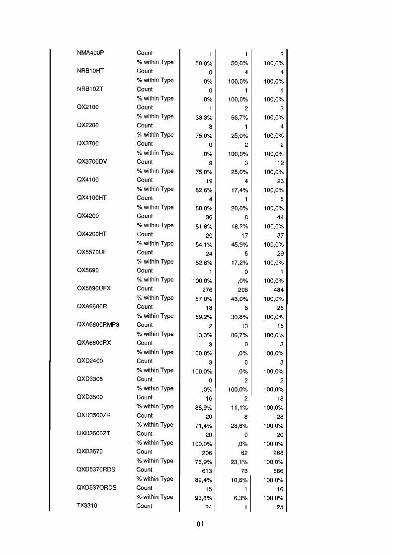
NMA400P Count 2% within Type 50,0% 50,0% 100,0%

NRB10HT Count ° 4 4% within Type ,0% 100,0% 100,0%

NRB10ZT Count ° 1 1% within Type ,0% 100,0% 100,0%

QX21 00 Count 2 3% within Type 33,3% 66,7% 100,0%

QX2200 Count 3 1 4% within Type 75,0% 25,0% 100,0%

QX3700 Count ° 2 2% within Type ,0% 100,0% 100,0%

QX3700DV Count 9 3 12% within Type 75,0% 25,0% 100,0%

QX41 00 Count 19 4 23% within Type 82,6% 17,4% 100,0%

QX4100HT Count 4 1 5% within Type 80,0% 20,0% 100,0%

QX4200 Count 36 8 44% within Type 81,8% 18,2% 100,0%

QX4200HT Count 20 17 37% within Type 54,1% 45,9% 100,0%

QX5570UF Count 24 5 29% within Type 82,8% 17,2% 100,0%

QX5690 Count 1 ° 1% within Type 100,0% ,0% 100,0%

QX5690UFX Count 276 208 484% within Type 57,0% 43,0% 100,0%

QXA6600R Count 18 8 26% within Type 69,2% 30,8% 100,0%

QXA6600RMP3 Count 2 13 15% within Type 13,3% 86,7% 100,0%

QXA6600RX Count 3 ° 3% within Type 100,0% ,0% 100,0%

QXD2400 Count 3 ° 3% within Type 100,0% ,0% 100,0%

QXD3305 Count ° 2 2% within Type ,0% 100,0% 100,0%

QXD3500 Count 16 2 18% within Type 88,9% 11,1% 100,0%

QXD3500ZR Count 20 8 28% within Type 71,4% 28,6% 100,0%

QXD3500ZT Count 20 ° 20% within Type 100,0% ,0% 100,0%

QXD3570 Count 206 62 268% within Type 76,9% 23,1% 100,0%

QXD5370RDS Count 613 73 686% within Type 89,4% 10,6% 100,0%

QXD5370RDS Count 15 16% within Type 93,8% 6,3% 100,0%

TX331° Count 24 25

101

Total

% within Type

Count

% within Type

96,0%

1685

71,2%

4,0%

681

28,8%

100,0%

2366

100,0%

Table 4.10.: Repair percentage for audio-sets

Repair department Total

DVD-player Yes NoType ADR5800DI Count 4 ° 4

% within Type 100,0% ,0% 100,0%DVP341° Count

° 1 1% within Type ,00/0 100,0% 100,0%

DVP3470SK Count 1 1 2% within Type 50,0% 50,0% 100,0%

DVP3550S Count 1 ° 1% within Type 100,0% ,0% 100,0%

DVP4330S Count 3 11 14% within Type 21,4% 78,6% 100,0%

DVP4330SBOXF Count 1 9 10% within Type 10,0% 90,0% 100,0%

DVP4330SBOXN Count 1 1 2% within Type 50,0% 50,0% 100,0%

DVP4410 Count° 1 1

% within Type ,0% 100,0% 100,0%DVP4420S Count

° 10 10% within Type ,0% 100,0% 100,0%

DVP4420SBW Count 1 5 6% within Type 16,7% 83,3% 100,0%

DVP4420SBWCF Count° 2 2

% within Type ,0% 100,0% 100,0%DVP4580SL Count 81 46 127

% within Type 63,8% 36,2% 100,0%DVP5380S Count 86 19 105

% within Type 81,9% 18,1% 100,0%DVP5380SBOXF Count 9 11 20

% within Type 45,0% 55,0% 100,0%DVP5380SBOXN Count 92 11 103

% within Type 89,3% 10,7% 100,0%DVP5388S Count 42 31 73

% within Type 57,5% 42,5% 100,0%DVPX7580 Count 18 22 40

% within Type 45,0% 55,0% 100,0%DVX2880 Count 9 ° 9

% within Type 100,0% ,0% 100,0%EDX6100 Count

° 1 1% within Type ,00/0 100,0% 100,0%

NDV150 Count 11 63 74% within Type 14,9% 85,1% 100,0%

NDV160 Count 57 248 305% within Type 18,7% 81,3% 100,0%

NDV210 Count 3 6 9% within Type 33,3% 66,7% 100,0%

102

NDV220 Count 25 49 I 74% within Type 33,8% 66,2% 100,0%

Total Count 445 548 993% within Type 44,8% 55,2% 100,0%

Table 4.11.: Repair percentage for DVD-p1ayers

KTV DVD/Video Repair department Total

combi Yes NoType CTR141MTV Count 12 0 12

% within Type 100,0% ,0% 100,0%CTR21MT4V Count 5 1 6

% within Type 83,3% 16,7°/<, 100,0%CTS141MTD Count 23 1 24

% within Type 95,8% 4,2% 100,0%CTS141 MTDE3 Count 126 14 140

% within Type 90,0% 10,0% 100,0%CTS14MTDE3 Count 20 0 20

% within Type 100,0% ,0% 100,0%CTS211MTD Count 87 10 97

% within Type 89,7% 10,3% 100,0%CTS21 MTDE3 Count 80 ~l 83

% within Type 96,4% 3,6% 100,0%DVV605N Count 2 0 2

% within Type 100,0% ,0% 100,0%DVV606N Count 32 1 33

% within Type 97,0% 3,0% 100,0%NDVCR300 Count 270 101 371

% within Type 72,8% 27,2% 100,0%NTDV14 Count 114 2,' 141

% within Type 80,9% 19,1% 100,0%NTDV21 Count 6 8 14

% within Type 42,9% 57,1% 100,0%Total Count 777 16Ei 943

% within Type 82,4% 17,6% 100,0%

Table 4.12.: RepaIr percentage for KTV DVDNldeo combl

Repair department Total

Home Cinema Yes NoType AM810 Count 1 ° 1

% within Type 100,0% ,0% 100,0%AX700 Count 1 ° 1

% within Type 100,0% ,0% 100,0%

AX81° Count 1 ° 1% within Type 100,0% ,0% 100,0%

CMB4300SS Count 13 ° 13% within Type 100,0% ,0% 100,0%

CX4200 Count 1 ° 1% within Type 100,0% ,0% 100,0%

DRR5800PST Count 20 2 22% within Type 90,9% 9,1% 100,0%

DVR2120 Count 1 ° 1

103

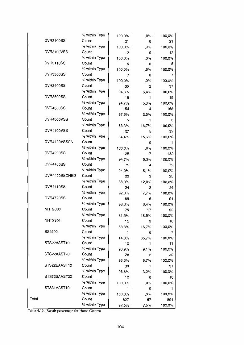
% within Type 100,0% ,0% 100,0%DVR3100SS Count 21 ° 21

% within Type 100,0% ,0% 100,0%DVR3100VSS Count 12 ° 12

% within Type 100,0% ,0% 100,0%DVR3110SS Count 5 ° 5

% within Type 100,0% ,0% 100,0%DVR3300SS Count 7 ° 7

% within Type 100,0% ,0% 100,0%DVR3400SS Count 35 2 37

% within Type 94,6% 5,4% 100,0%DVR3500SS Count 18 1 19

% within Type 94,7% 5,3% 100,0%DVR4000SS Count 154 4 158

% within Type 97,5% 2,5% 100,0%DVR4000VSS Count 5 1 6

% within Type 83,3% 16,7% 100,0%DVR4100VSS Count 27 5 32

% within Type 84,4% 15,6% 100,0%DVR4100VSSCN Count 1 ° 1

% within Type 100,0% ,0% 100,0%DVR4200SS Count 125 7 132

% within Type 94,7% 5,3% 100,0%DVR4400SS Count 75 4 79

% within Type 94,9% 5,1% 100,0%DVR4400SSCNED Count 22 3 25

% within Type 88,0% 12,0% 100,0%DVR4410SS Count 24 2 26

% within Type 92,3% 7,7% 100,0%DVR4720SS Count 88 6 94

% within Type 93,6% 6,4% 100,0%NHTS300 Count 75 17 92

% within Type 81,5% 18,5% 100,0%NHTS301 Count 15 3 18

% within Type 83,3% 16,7% 100,0%SS4500 Count 1 6 7

% within Type 14,3% 85,7% 100,0%STS22AAST1° Count 10 1 11

% within Type 90,9% 9,1% 100,0%STS22AAST20 Count 28 2 30

% within Type 93,3% 6,7% 100,0%STS22EAAST10 Count 30 1 31

% within Type 96,8% 3,2% 100,0%STS22SAAST20 Count 10 ° 10

% within Type 100,0% ,0% 100,0%STS31AAST10 Count 1 ° 1

% within Type 100,0% ,0% 100,0%Total Count 827 67 894

% within Type 92,5% 7,5% 100,0%

Table 4.13.: RepaIr percentage for Home Cmema

104

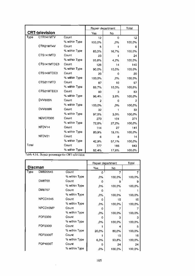
Table 4.14.: RepaIr percentage for CRT-televIsion

Repair department Total

CRT-television Yes NoType CTR141MTV Count 12 0 12

% within Type 100,0% ,0% 100,0%CTR21 MT4V Count 5 1 6

% within Type 83,3% 16,7% 100,0%CTS141MTD Count 23 1 24

% within Type 95,8% 4,2% 100,0%CTS141 MTDE3 Count 126 14 140

% within Type 90,0% 10,0% 100,0%CTS14MTDE3 Count 20 0 20

% within Type 100,0% ,0% 100,0%CTS211MTD Count 87 10 97

% within Type 89,7% 10,3% 100,0%CTS21MTDE3 Count 80 3 83

% within Type 96,4% 3,6% 100,0%DVV605N Count 2 0 2

% within Type 100,0% ,0% 100,0%DVV606N Count 32 1 33

% within Type 97,0% 3,0% 100,0%NDVCR300 Count 270 101 371

% within Type 72,8% 27,2% 100,0%NTDV14 Count 114 27 141

% within Type 80,9% 19,1% 100,0%NTDV21 Count 6 8 14

% within Type 42,9% 57,1% 100,0%Total Count 777 166 943

% within Type 82,4% 17,6% 100,0%..

- Repair department Total

Discman Yes NoType DM820545 Count 0 7 7

% within Type ,0% 100,0% 100,0%DM8700 Count 0 9 9

% within Type ,0% 100,0% 100,0%DM8707 Count 0 1 1

% within Type ,0% 100,0% 100,0%NPCD1045 Count 0 15 15

% within Type ,0% 100,0% 100,0%NPCD10MP Count 0 7 7

% within Type ,0% 100,0% 100,0%PDP2300 Count 0 3 3

% within Type ,0% 100,0% 100,0%PDP23001 Count 1 4 5

% within Type 20,0% 80,0% 100,0%PDP2300T Count 1 15 16

% within Type 6,3% 93,8% 100,0%PDP4000T Count 0 24 24

% within Type ,0% 100,0% 100,0%

105

PDP4580SRBW Count 11 119 130% within Type 8,5% 91,5% 100,0%

PDP4580SROR Count ° 28 28% within Type ,0% 100,0% 100,0%

PDP4580SRZR Count 13 103 116% within Type 11,2% 88,8% 100,0%

PDX2210 Count ° 2 2% within Type ,0% 100,0% 100,0%

PDX22101 Count 6 66 72% within Type 8,3% 91,7% 100,0%

PDX2210lMKIDS Count ° 7 7% within Type ,0% 100,0% 100,0%

PDX3780 Count 1 15 16% within Type 6,3% 93,8% 100,0%

PDX4440 Count 1 ° 1% within Type 100,0% ,0% 100,0%

PDX4440R Count ° 5 5% within Type ,0% 100,0% 100,0%

Total Count 34 430 464% within Type 7,3% 92,7% 100,0%

Table 4.15.: Rep31r percentage for Dlscman

Repair department Total

Alarmclock Yes NoType AR4100 Count 1 35 36

% within Type 2,8% 97,2% 100,0%ARF360D Count ° 117 117

% within Type ,0% 100,0% 100,0%CD112AT Count ° 1 1

% within Type ,0% 100,0% 100,0%CD112GS Count ° 5 5

% within Type ,0% 100,0% 100,0%NCL7WT Count ° 8 8

% within Type ,0% 100,0% 100,0%NCL7ZR Count ° 15 15

% within Type ,0% 100,0% 100,0%NCR11ZR Count ° 12 12

% within Type ,0% 100,0% 100,0%NCR12WT Count ° 57 57

% within Type ,0% 100,0% 100,0%NCR12ZR Count ° 2 2

% within Type ,0% 100,0% 100,0%NCR24WT Count ° 1 1

% within Type ,0% 100,0% 100,0%NCR25ZR Count ° 1 1

% within Type ,0% 100,0% 100,0%NCR32ZR Count ° 1 1

% within Type ,0% 100,0% 100,0%NCR33WT Count ° 26 26

% within Type ,0% 100,0% 100,0%NCR33ZT Count ° 36 36

106

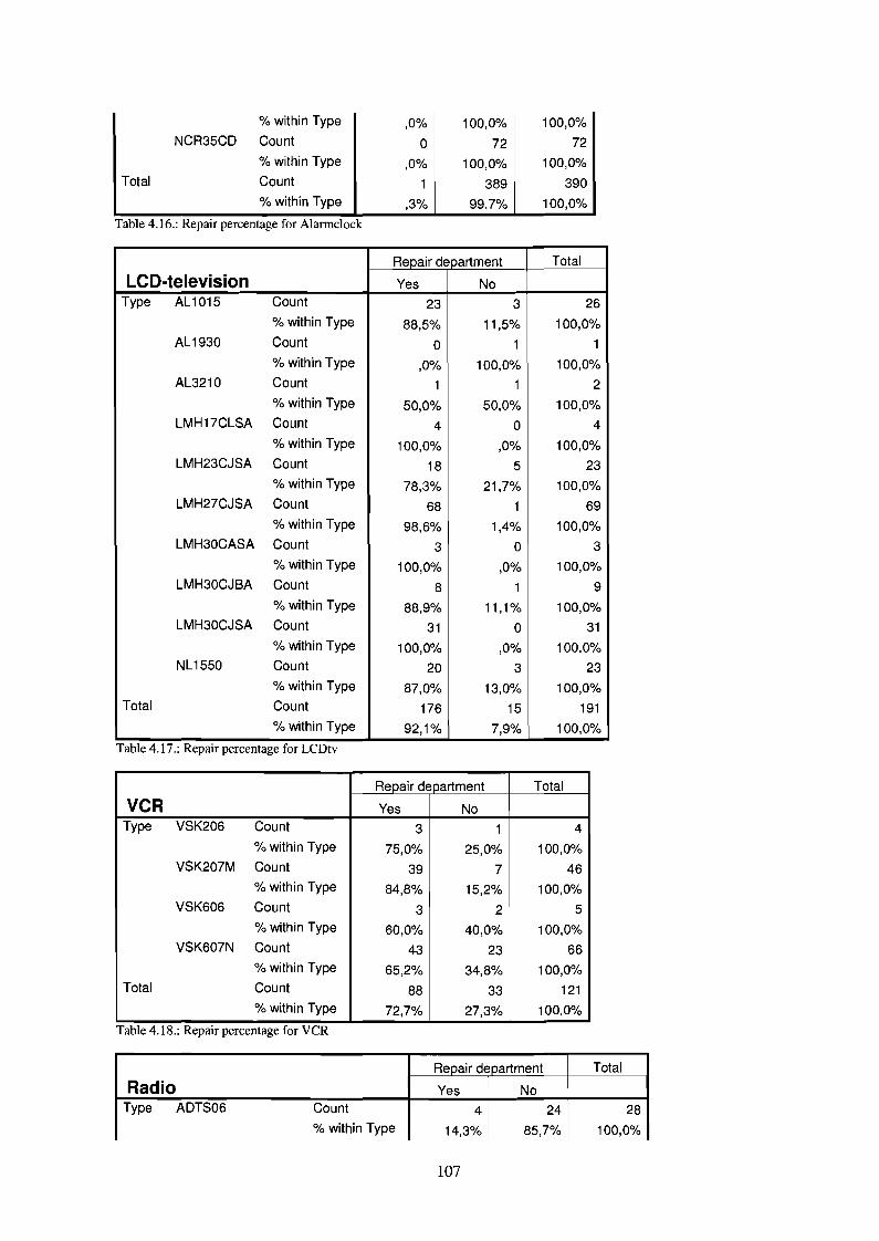
% within Type ,0% 100,0% 100,0%NCR35CD Count ° 72 72

% within Type ,0% 100,0% 100,0%Total Count 389 390

% within Type ,3% 99,7% 100,0%

Table 4.16.: Repair percentage for Alarmclock

Repair department Total

LCD-television Yes NoType AL1015 Count 23 3 26

% within Type 88,5% 11,5% 100,0%AL1930 Count ° 1 1

% within Type ,0% 100,0% 100,0%AL3210 Count 1 1 2

% within Type 50,0% 50,0% 100,0%LMH17CLSA Count 4 ° 4

% within Type 100,0% ,0% 100,0%LMH23CJSA Count 18 5 23

% within Type 78,3% 21,7% 100,0%LMH27CJSA Count 68 1 69

% within Type 98,6% 1,4% 100,0%LMH30CASA Count 3 ° 3

% within Type 100,0% ,0% 100,0%LMH30CJBA Count 8 1 9

% within Type 88,9% 11,1% 100,0%LMH30CJSA Count 31 ° 31

% within Type 100,0% ,0% 100,0%NL1550 Count 20 3 23

% within Type 87,0% 13,0% 100,0%Total Count 176 15 191

% within Type 92,1% 7,9% 100,0%

Table 4.17.: Repan percentage for LCDtv

Repair department Total

VCR Yes NoType VSK206 Count 3 1 4

% within Type 75,0% 25,0% 100,0%VSK207M Count 39 7 46

% within Type 84,8% 15,2% 100,0%VSK606 Count 3 2 5

% within Type 60,0% 40,0% 100,0%VSK607N Count 43 23 66

% within Type 65,2% 34,8% 100,0%Total Count 88 33 121

% within Type 72,7% 27,3% 100,0%

Table 4.18.: Repan percentage for VCR

Repair deoartment Total

Radio Yes NoType ADTS06 Count 4 24 28

% within Type 14,3% 85,7% 100,0%

107

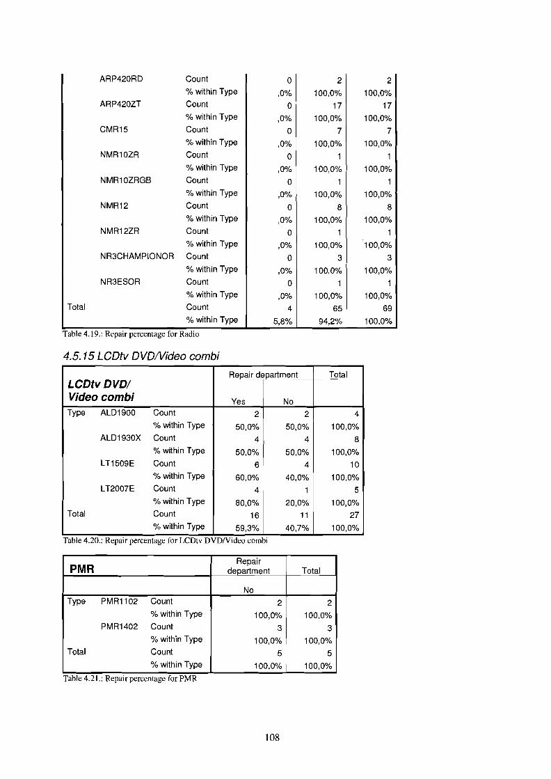
ARP420RD Count ° 2 2% within Type ,0% 100,0% 100,0%

ARP420ZT Count ° 17 17% within Type ,0% 100,0% 100,0%

CMR15 Count ° 7 7% within Type ,0% 100,0% 100,0%

I\JMR10ZR Count ° 1 1% within Type ,0% 100,0% 100,0%

NMR10ZRGB Count ° 1 1% within Type ,0% 100,0% 100,0%

NMR12 Count ° 8 8% within Type ,0% 100,0% 100,0%

NMR12ZR Count ° 1 1% within Type ,0% 100,0% 100,0%

NR3CHAMPIONOR Count ° 3 3% within Type ,0% 100,0% 100,0%

NR3ESOR Count ° 1 1% within Type ,0% 100,0% 100,0%

Total Count 4 65 69% within Type 5,8% 94,2% 100,0%

Table 4.19.: Repair percentage for RadIO

4.5.15 LCDtv DVDIVideo combi

Repair djPartment TotalLCDtvDVDIVideo combi Yes NoType ALD1900 Count 2 2 4

% within Type 50,0% 50,0% 100,0%ALD1930X Count 4 4 8

% within Type 50,0% 50,0% 100,0%LT1509E Count 6 4 10

% within Type 60,0% 40,0% 100,0%LT2007E Count 4 1 5

% within Type 80,0% 20,0% 100,0%Total Count 16 11 27

% within Type 59,3% 40,7% 100,0%

Table 4.20.: Repair percentage for LCDtv DVDNldeo combl

PMRRepair

department Total

NoType PMR1102 Count 2 2

% within Type 100,0% 100,0%PMR1402 Count 3 3

% within Type 100,0% 100,0%Total Count 5 5

% within Type 100,0% 100,0%

Table 4.21.: Repalf percentage for PMR

108

Appendix 4.3: Number of repaired warranty returns

4.3.1. Number of repaired warranty returns per month in 2006

1.000

800

~ 600CCI)::::J

WLL

400

200

o 2 4 6 8 10 12

Fig. 4.13. The frequency of repair under warranty per month, month 1 starts 1 February

Appendix 4.4: The failure behavior of to be repaired warranty returns

4.4. 1. Failure behavior combinations for the product groupsThe tables below show the combination of failure section, type of failure and type of repair as

expressed in the IRIS-codes. The codes displayed consist of the three IRIS-code parts joined together.The IRIS-code classification table is shown in Appendix 3.1. When codes that are only observed threeor less times and together are responsible for less then 35% of the returns they are grouped underother.

The colums in the tables, from left to right, indicate the IRIScode, the frequency that it wasobserved, the percentage of the total number of observations for the product group and the cumulativepercentage of the total repairs accounted for.

Audio-setCumulative

Freauency Percent PercentIRIScode: DDMNA

277 16,4 16,4PSUNA 119 7,1 23,5SYSOL

105 6,2 29,7DDM3M 97 5,8 35,5DDMOA 87 5,2 40,7APDNA

72 4,3 44,9DDMCS 58 3,4 48,4SYSOA 57 3,4 51,8

109

APA3M34 2,0 53,8

PSU3M 29 1,7 55,503L 28 1,7 57,2DDM2Z 24 1,4 58,6DDM3L 23 1,4 59,9IDSNA 22 1,3 61,2REMOA 22 1,3 62,6APANA 21 1,2 63,8CTRNA 21 1,2 65,0SYSOC 20 1,2 66,2APD2A 18 1,1 67,3SYS2A 16 ,9 68,2PSUOA 15 ,9 69,1TDMNA 15 ,9 70,0HFS3M 12 ,7 70,7PSU2G 12 ,7 71,5TDMOA 12 ,7 72,2DDMNZ 11 ,7 72,8OOA 10 ,6 73,4APAOA 10 ,6 74,0HFSRD 10 ,6 74,6SYSID 10 ,6 75,2SYSPC 10 ,6 75,8APARD 9 ,5 76,3REMNA 9 ,5 76,9DNA 8 ,5 77,3APA2A

8 ,5 77,8DDMBE 8 ,5 78,3IDSOA 8 ,5 78,8IDS3M 8 ,5 79,2PSUOG 8 ,5 79,7DDMCA 7 ,4 80,1DDMDA 7 ,4 80,5SYSOG 7 ,4 80,9TUN3L 7 ,4 81,403M 6 ,4 81,7DDM1Z 6 ,4 82,1DDMTD

6 ,4 82,4HFSNA

6 ,4 82,8PSUID 6 ,4 83,1TDMCB 6 ,4 83,5APA2Z 5 ,3 83,8CBTOA 5 ,3 84,1CBTDA 5 ,3 84,4

110

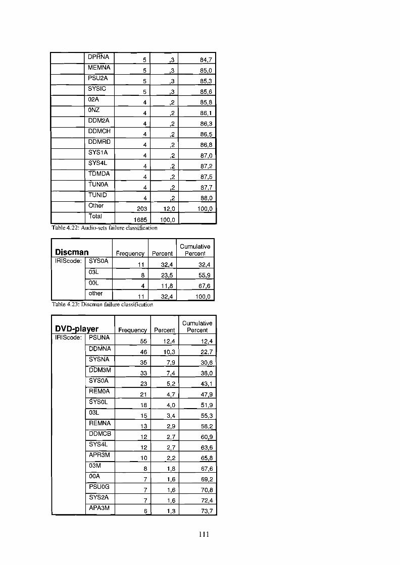
DPRNA 5 ,3 84,7MEMNA 5 ,3 85,0PSU2A 5 ,3 85,3SYSIC

5 ,3 85,602A 4 ,2 85,8ONZ

4 ,2 86,1DDM2A 4 ,2 86,3DDMCH 4 ,2 86,5DDMRD 4 ,2 86,8SYS1A 4 ,2 87,0SYS4L 4 ,2 87,2TDMDA 4 ,2 87,5TUNOA 4 ,2 87,7TliNID

4 ,2 88,0Other 203 12,0 100,0Total

1685 100,0Table 4.22: AudIO-sets faIlure classIfication

CumulativeDiscman Frequency Percent PercentIRIScode: SYSOA

11 32,4 32,403L

8 23,5 55,9OOL 4 11,8 67,6other

11 32,4 100,0Table 4.23: Dlscman faIlure classIficatIOn

CumulativeDVD-player Frequency Percent PercentIRIScode: PSUNA

55 12,4 12,4DDMNA

46 10,3 22,7SYSNA 35 7,9 30,6DDM3M 33 7,4 38,0SYSOA 23 5,2 43,1REMOA

21 4,7 47,9SYSOL

18 4,0 51,903L 15 3,4 55,3REMNA 13 2,9 58,2DDMCS 12 2,7 60,9SYS4L 12 2,7 63,6APR3M 10 2,2 65,803M 8 1,8 67,6OOA 7 1,6 69,2PSUOG 7 1,6 70,8SYS2A

7 1,6 72,4APA3M

6 1,3 73,7

111

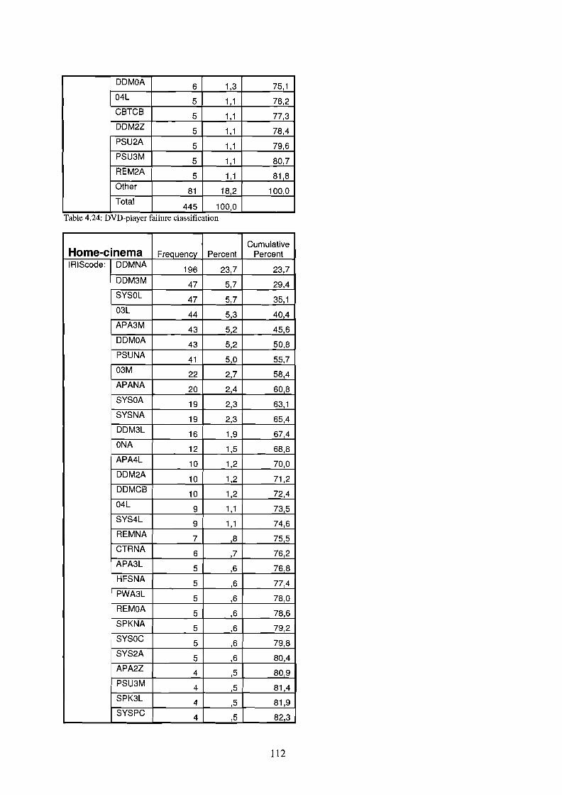
DDMOA6 1,3 75,1

04L 5 1,1 76,2CSTCS 5 1,1 77,3DDM2Z 5 1,1 78,4PSU2A 5 1,1 79,6PSU3M 5 1,1 80,7REM2A 5 1,1 81,8Other

81 18,2 100,0Total

445 100,0Table 4.24: DVD-player fmlure classIficatIOn

CumulativeHome-cinema Frequency Percent PercentIRIScode: DDMNA

196 23,7 23,7DDM3M 47 5,7 29,4SYSOL 47 5,7 35,103L 44 5,3 40,4APA3M

43 5,2 45,6DDMOA 43 5,2 50,8PSUNA 41 5,0 55,703M 22 2,7 58,4APANA 20 2,4 60,8SYSOA 19 2,3 63,1SYSNA 19 2,3 65,4DDM3L 16 1,9 67,4ONA 12 1,5 68,8APA4L 10 1,2 70,0DDM2A

10 1,2 71,2DDMCS 10 1,2 72,404L

9 1,1 73,5SYS4L 9 1,1 74,6REMNA 7 ,8 75,5CTRNA 6 ,7 76,2APA3L 5 ,6 76,8HFSNA 5 ,6 77,4PWA3L 5 ,6 78,0REMoA 5 ,6 78,6SPKNA 5 ,6 79,2SYSOC 5 ,6 79,8SYS2A 5 ,6 80,4APA2Z 4 ,5 80,9PSU3M 4 ,5 81,4SPK3L 4 ,5 81,9SYSPC 4 ,5 82,3

112

Other 143 17,7 100Total

827 100,0Table 4.25: Home-cmema failure classIficatIOn

CRT DVD/Cumulative

Video combi Freauencv Percent PercentIRIScode: DDMNA

198 25,5 25,5PSlINA

97 12,5 38,0DDM3M

68 8,8 46,703L

55 7,1 53,8DDM3L

50 6,4 60,2SYSOL 31 4,0 64,2DDMSE

21 2,7 66,9REMNA

20 2,6 69,5SYS4L 18 2,3 71,8PSU3M

15 1,9 73,7TDM3M 14 1,8 75,5ONA

12 1,5 77,1DDMCS

10 1,3 78,4CTRNA 9 1,2 79,5SYSOA

8 1,0 80,6DFLNA 7 ,9 81,5TDMNA

6 ,8 82,204L 5 ,6 82,9ONZ

5 ,6 83,5DDMOA

5 ,6 84,2HFSNA 5 ,6 84,8REM2A 5 ,6 85,5OOA 4 ,5 86,0HFS3M 4 ,5 86,5TDMCS

4 ,5 87,0Other 101 13,0 100,0Total

777 100,0Table 4.26: CRT DVD/vldeo combl failure classIficatIOn

CRT-Cumulative

television Frequency Percent PercentIRIScode: PSUNA

145 23,6 23,603L

37 6,0 29,6SYSOL 30 4,9 34,5ONA

26 4,2 38,7DFLNA

21 3,4 42,1PSU3M

17 2,8 44,9REMNA

16 2,6 47,5PSU2A

12 2,0 49,4

113

Table 4.27: CRT-televIsIOn faIlure classificatIOn

SYS2A 12 2,0 51,4APA3M 11 1,8 53,2CPANA 11 1,8 55,0PSUOG 11 1,8 56,7PSUID 11 1,8 58,5SYSPC 11 1,8 60,3DFL3M 10 1,6 62,0PSU2G 10 1,6 63,6REMOA 10 1,6 65,2SYSOA 10 1,6 66,8SYSOC 10 1,6 68,5APANA

9 1,5 69,9DFLCB 7 1,1 71,1HFSNA 7 1,1 72,2SYS1C 7 1,1 73,3PSUOD 6 1,0 74,3SYS1A 6 1,0 75,3APA2A

5 ,8 76,1CPA3M

5 ,8 76,9HFS3M 5 ,8 77,7PSUOA 5 ,8 78,5PSURD 5 ,8 79,302A 4 ,7 80,0APAOA 4 ,7 80,7APAPG 4 ,7 81,3TUNNA 4 ,7 82,0Other 111 18,0 100,0Total

615 100,0..

LCDtv DVDI CumulativeVideo combi Frequency Percent PercentIRIScode: 03L 3 18,8 18,8

DDMNA 3 18,8 37,5

04L 1 6,3 43,8

ONZ 1 6,3 50,0ANT1Z 1 6,3 56,3APANZ 1 6,3 62,5

DDMoo 1 6,3 68,8

DDM1Z 1 6,3 75,0

DDM3M 1 6,3 81,3

HFS3M 1 6,3 87,5

PSU3M 1 6,3 93,8

SYS01 1 6,3 100,0Total 16 100,0

Table 4.28: LCDtv DVD combl failure classificatIOn

114

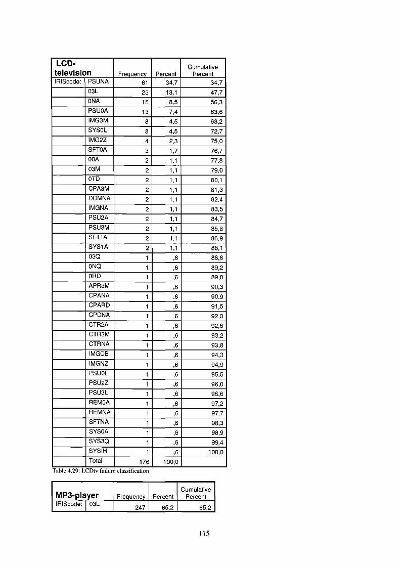
LCD- Cumulativetelevision Frequency Percent PercentIRIScode: PSUNA 61 34,7 34,7

03L 23 13,1 47,7

ONA 15 8,5 56,3

PSUOA 13 7,4 63,6

IMG3M 8 4,5 68,2

SYSOL 8 4,5 72,7

IMG2Z 4 2,3 75,0

SFTOA 3 1,7 76,7

OOA 2 1,1 77,8

03M 2 1,1 79,0

OTO 2 1,1 80,1

CPA3M 2 1,1 81,3

OOMNA 2 1,1 82,4

IMGNA 2 1,1 83,5

PSU2A 2 1,1 84,7

PSU3M 2 1,1 85,8

SFT1A 2 1,1 86,9

SYS1A 2 1,1 88,1

03Q 1 ,6 88,6

ONQ 1 ,6 89,2

ORO 1 ,6 89,8

APR3M 1 ,6 90,3

CPANA 1 ,6 90,9

CPARO 1 ,6 91,5

CPONA 1 ,6 92,0

CTR2A 1 ,6 92,6

CTR3M 1 ,6 93,2

CTRNA 1 ,6 93,8

IMGCB 1 ,6 94,3

IMGNZ 1 ,6 94,9

PSUOL 1 ,6 95,5

PSU2Z 1 ,6 96,0

PSU3L 1 ,6 96,6

REMOA 1 ,6 97,2

REMNA 1 ,6 97,7

SFTNA 1 ,6 98,3

SYSOA 1 ,6 98,9

SYS3Q 1 ,6 99,4

SYSIH 1 ,6 100,0

Total 176 100,0

Table 4.29: LCDtv fmlure classlficatlOn

CumulativeMP3-player Frequency Percent PercentIRIScode: I03L

247 65,2 65,2

115

SYSOA 55 14,5 79,7SYSOL 17 4,5 84,2IDSOA 12 3,2 87,3SYSOC 7 1,8 89,2OOL

6 1,6 90,802A

6 1,6 92,3Other 29 7,7 100,0Total

379 100,0Table 4.30: MP3 player faIlure classificatIOn

Portable LCD CumulativeDVD player Frequency Percent PercentIRIScode: DDMOA 259 11,5 11,5

SYSOL 250 11,1 22,5SYSOA 217 9,6 32,1DDMNA 144 6,4 38,5IDSOA 140 6,2 44,7PSUNA 126 5,6 50,2DDMCB 91 4,0 54,2PSUOA 58 2,6 56,8DDM3M 57 2,5 59,3SYS4L 54 2,4 61,7DDMBE 53 2,3 64,1IMGNA 42 1,9 65,9IDSNA 38 1,7 67,6SYSOC 35 1,5 69,1PSU2A 30 1,3 70,5PSU3M 30 1,3 71,8EXCOA 28 1,2 73,0IDS3M 26 1,1 74,2PSUOG 24 1,1 75,2SYS2A 20 ,9 76,1REMOA 19 ,8 77,0ONA 18 ,8 77,8DDMOB 18 ,8 78,6DDMOE 15 ,7 79,2IMG3M 15 ,7 79,9DDM1A 14 ,6 80,5PSU2G 13 ,6 81,1IDS2A 12 ,5 81,6SYSOG 12 ,5 82,1OOA 11 ,5 82,6CBTOA 11 ,5 83,1

116

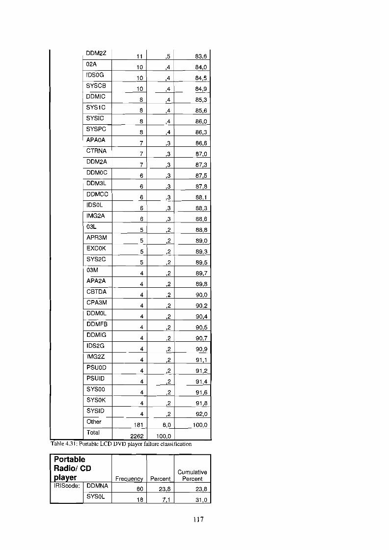
I DDM2Z11 ,5 83,6

02A 10 ,4 84,0IDSOG 10 ,4 84,5SYSCB 10 ,4 84,9DDMIC

8 ,4 85,3SYS1C 8 ,4 85,6SYSIC

8 ,4 86,0SYSPC

8 ,4 86,3APAOA 7 ,3 86,6CTRNA 7 ,3 87,0DDM2A 7 ,3 87,3DDMOC 6 ,3 87,5DDM3L

6 ,3 87,8DDMCC 6 ,3 88,1IDSOL

6 ,3 88,3IMG2A 6 ,3 88,603L

5 ,2 88,8APR3M 5 ,2 89,0EXCOK

5 ,2 89,3SYS2C

5 ,2 89,503M 4 ,2 89,7APA2A 4 ,2 89,8CBTDA 4 ,2 90,0CPA3M 4 ,2 90,2DDMOL 4 ,2 90,4DDMFB 4 ,2 90,5DDMIG 4 ,2 90,7IDS2G 4 ,2 90,9IMG2Z 4 ,2 91,1PSUOD 4 ,2 91,2PSUID 4 ,2 91,4SYSOO 4 ,2 91,6SYSOK 4 ,2 91,8SYSID 4 ,2 92,0Other

181 8,0 100,0Total

2262 100,0Table 4.31: Portable LCD DVD player faIlure classIfication

PortableRadio/ CD Cumulativeplayer Freauency Percent PercentIRIScode: DDMNA

60 23,8 23,8SYSOL

18 7,1 31,0

117

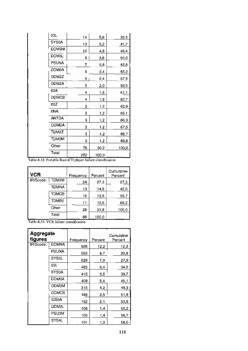
03L 14 5,6 36,5SYSOA 13 5,2 41,7DDM3M 12 4,8 46,4DDM3L 9 3,6 50,0PSUNA 7 2,8 52,8DDMOA 6 2,4 55,2DDM2Z 6 2,4 57,5DDM2A 5 2,0 59,502A 4 1,6 61,1DDMCS 4 1,6 62,702Z

3 1,2 63,9ONA

3 1,2 65,1ANTDA 3 1,2 66,3DDMDA 3 1,2 67,5TDM2Z 3 1,2 68,7TDM3M 3 1,2 69,8Other 76 30,2 100,0Total

252 100,0Table 4.32: Portable RaclOCD player fallure classIficatIOn

CumulativeVCR Freauencv Percent PercentIRIScode: TDM3M 24 27,3 27,3

TDMNA 13 14,8 42,0TDMCS 12 13,6 55,7TDMSE 11 12,5 68,2Other 28 31,8 100,0Total

88 100,0Table 4.33: VCR fallure classIficatIOn

Aggregate Cumulativefigures Freauency Percent PercentIRIScode: I DDMNA 926 12,2 12,2

I PSUNA 655 8,7 20,9SYSOL 529 7,0 27,903L 483 6,4 34,2SYSOA 415 5,5 39,7DDMOA 409 5,4 45,1DDM3M 315 4,2 49,3DDMCS 186 2,5 51,8IDSOA 162 2,1 53,9DDM3L 106 1,4 55,3PSU3M 105 1,4 56,7SYS4L 101 1,3 58,0

118

APA3M 99 1,3 59,3ONA 97 1,3 60,6PSUOA 94 1,2 61,8DDMBE 87 1,1 63,0REMOA 84 1,1 64,1SYSOC 83 1,1 65,2APDNA 76 1,0 66,2REMNA 67 ,9 67,1IDSNA 63 ,8 67,9SYS2A 63 ,8 68,7SYSNA 61 ,8 69,6PSU2A 58 ,8 70,3PSUOG 55 ,7 71,0APANA 54 ,7 71,8DDM2Z 52 ,7 72,4CTRNA 50 ,7 73,1IMGNA 48 ,6 73,703M 46 ,6 74,3TDM3M 44 ,6 74,9OOA 38 ,5 75,4IDS3M 37 ,5 75,9PSU2G 36 ,5 76,4TDMNA 35 ,5 76,9SYSPC 34 ,4 77,3EXCOA 31 ,4 77,702A 30 ,4 78,104L 30 ,4 78,5DDM2A 30 ,4 78,9PSUID 29 ,4 79,3DFLNA 28 ,4 79,7IMG3M 26 ,3 80,0HFS3M 25 ,3 80,3APAOA 24 ,3 80,6HFSNA 24 ,3 81,0DDMOB 23 ,3 81,3SYSOG 23 ,3 81,6TDMCB 22 ,3 81,9APD2A 21 ,3 82,1APR3M 21 ,3 82,4APA2A 20 ,3 82,7ONZ 19 ,3 82,9CBTOA 19 ,3 83,2

119

SYS1C19 ,3 83,4

SYSID 19 ,3 83,7DDMNZ 18 ,2 83,9TDMBE 18 ,2 84,2CPA3M 17 ,2 84,4DDM1A 17 ,2 84,6DDMOE 16 ,2 84,8SYSIC 15 ,2 85,002Z

14 ,2 85,2CPANA 14 ,2 85,4DDMDA 14 ,2 85,6REM2A 14 ,2 85,8SYS1A 14 ,2 85,9OOL 13 ,2 86,1APARD 13 ,2 86,3DDMCA 13 ,2 86,5DDMFB

13 ,2 86,6IDS2A 13 ,2 86,8TDMOA

13 ,2 87,0DFL3M 12 ,2 87,1PSUOD 12 ,2 87,3PSU3L 12 ,2 87,5TUN3L 12 ,2 87,6APA2Z 11 ,1 87,8CTR3M 11 ,1 87,9HFSRD 11 ,1 88,0IDSOG

11 ,1 88,2PSU2Z 11 ,1 88,3I

SPKNA 11 ,1 88,5APA4L 10 ,1 88,6DDMOL 10 ,1 88,7SYSCB 10 ,1 88,9CBTCB 9 ,1 89,0CBTDA 9 ,1 89,1DDM1Z

9 ,1 89,2DDMIC 9 ,1 89,4PSURD

9 ,1 89,5PWA3L 9 ,1 89,6IMG2Z 8 ,1 89,7SFTOA 8 ,1 89,8TDM2Z 8 ,1 89,9DDMOC 7 ,1 90,0

120

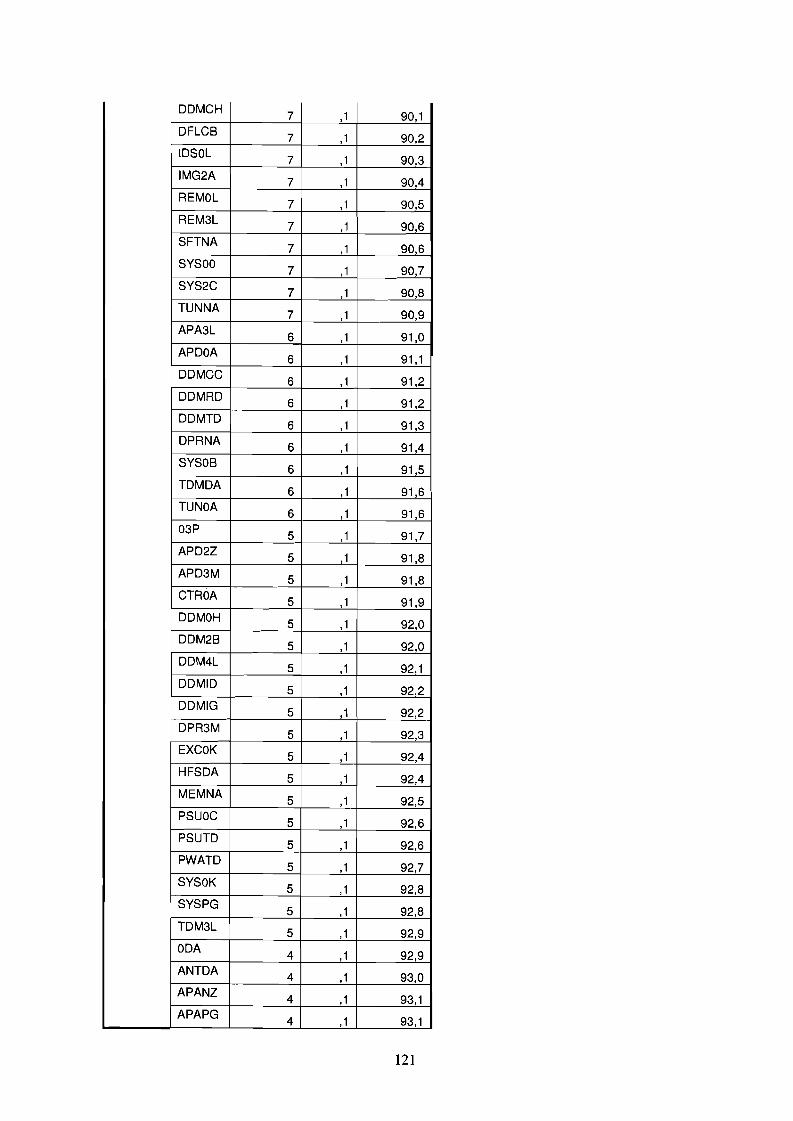
0 DMCH7 ,1 90,1

0 FLCB7 ,1 90,2

IDSOL7 ,1 90,3

IMG2A7 ,1 90,4

REMOL7 ,1 90,5

REM3L7 ,1 90,6

SFTNA7 ,1 90,6

SYSOO7 ,1 90,7

SYS2C7 ,1 90,8

TUNNA7 ,1 90,9

APA3L6 ,1 91,0

APDOA6 ,1 91,1

DDMCC6 ,1 91,2

DDMRD6 ,1 91,2

DDMTD6 ,1 91,3

DPRNA6 ,1 91,4

SYSOB6 ,1 91,5

TDMDA6 ,1 91,6

TUNOA6 ,1 91,6

03P5 ,1 91,7

APD2Z 5 ,1 91,8APD3M 5 ,1 91,8CTROA

5 ,1 91,9DDMOH

5 ,1 92,0DDM2B

5 ,1 92,0DDM4L

5 ,1 92,1DDMID

5 ,1 92,2DDMIG

5 ,1 92,2DPR3M

5 ,1 92,3EXCOK 5 ,1 92,4HFSDA

5 ,1 92,4MEMNA

5 ,1 92,SPSUOC

5 ,1 92,6PSUTD

5 ,1 92,6PWATD

5 ,1 92,7SYSOK

5 ,1 92,8SYSPG

5 ,1 92,8TDM3L 5 ,1 92,9ODA

4 ,1 92,9ANTDA

4 ,1 93,0APANZ

4 ,1 93,1APAPG

4 ,1 93,1

121

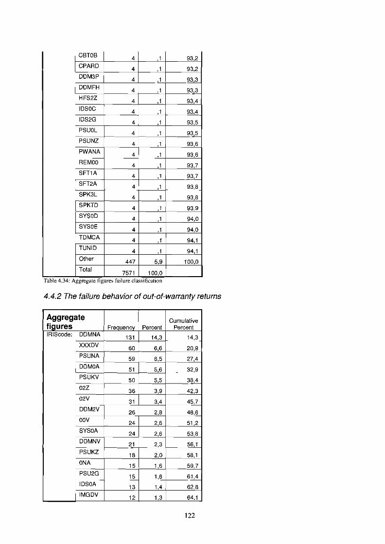
I CSTOS4 ,1 93,2

CPARO 4 ,1 93,2OOM3P 4 ,1 93,3OOMFH 4 ,1 93,3HFS2Z 4 ,1 93,4IOSOC 4 ,1 93,4IOS2G 4 ,1 93,5PSUOL 4 ,1 93,5PSUNZ 4 ,1 93,6PWANA 4 ,1 93,6REMOO 4 ,1 93,7SFT1A 4 ,1 93,7SFT2A 4 ,1 93,8SPK3L 4 ,1 93,8SPKTO 4 ,1 93,9SYSOO 4 ,1 94,0SYSOE 4 ,1 94,0TOMCA 4 ,1 94,1TUNIO 4 ,1 94,1Other 447 5,9 100,0Total

7571 100,0Table 4.34: Aggregate figures fmlure classIficatIOn

4.4.2 The failure behavior of out-of-warranty returns

Aggregate Cumulativefigures Frequency Percent PercentIRIScode: OOMNA 131 14,3 14,3

XXXOV 60 6,6 20,9PSUNA 59 6,5 27,4OOMOA 51 5,6 32,9PSUKV

50 5,5 38,402Z

36 3,9 42,302V 31 3,4 45,7OOM2V 26 2,8 48,6OOV 24 2,6 51,2SYSOA 24 2,6 53,8OOMNV 21 2,3 56,1PSUKZ 18 2,0 58,1ONA 15 1,6 59,7PSU2G 15 1,6 61,4IOSOA 13 1,4 62,8IMGOV 12 1,3 64,1

122

Table 4.35: Out of warranty failure classificatIOn

SYS2V12 1,3 65,4

XXXDZ 11 1,2 66,6DDM2A

10 1,1 67,7OOA 9 1,0 68,7OOY 9 1,0 69,7PSUOA 9 1,0 70,703L

8 ,9 71,6PSU2A 8 ,9 72,4TUNNA 7 ,8 73,2XXXGZ 7 ,8 74,0PSUNV

6 ,7 74,6SYS2Z 6 ,7 75,3XXXGV

6 ,7 75,9DDM2Z

5 ,5 76,5DDMDV

5 ,5 77,0IMGDZ

5 ,5 77,6SYSOY

5 ,5 78,1TDMNA

5 ,5 78,7ODV

4 ,4 79,1OKV

4 ,4 79,5CBT2A 4 ,4 80,0CBTDA 4 ,4 80,4DVD2V 4 ,4 80,9HFSNA 4 ,4 81,3SYS2A 4 ,4 81,7SYSKV 4 ,4 82,2Other 163 17,8 100,0Total

914 100,0

123

Appendix 12

In this Appendix the models used in the simulation are displayed. The graphic representation of themodels is displayed in Appendix 12.1 to 12.3. The arrival page is identical for all three designs. Therepair page is identical for design 1 and 2. Both are shown in Appendix 12.1. Appendix 12.4 containsthe declarations used in the models. These declaration were varied between models to obtain thesimulated scenarios. The variations are available at the author upon request.The used symbols in the figures representing the following:

Ellipses:Places, in a place something is stored. This something can be a person or product or administrativeobject, value etc. Each place can store certain things, depending on how the place is defined. This wayeg persons do not get mixed with products.

Squares:Transitions, a transition performs an action. To do so it requires objects from places. After the actionobjects are sent to the same or other places for storage agains. The action can represent anything fromthe periodic calculation of a formula to the transport or repair of a product. The actions can only beperformed if the right objects for the action are in the places connected to the transition. With theaction also a time delay can be defined.

Arrows:Arrows connect the places with the transitions, on the arrows it is defined what goes in transitions andwhat comes out of them and in which place it is then stored again.

Declarations:In the declarations all variables and formula's are defined. The abbreviations used for places,transitions and arrows are defined there.

Hierarchy: super and subpagesTo allow for a complex model to be readable the concept of hierarchy is used. With this conceptseveral transitions and places can be displayed as one transition. This transition then represents theunderlying structure on the superpage, whilst the structure of places and transitions is shown on thesubpage.

124

Appendix 12.1. Design 1

Appendix 12.1.1. The total model (superpage)

125

Appendix 12. 1.2. Arrive (subpage)

126

Appendix 12.1.3: Select (subpage)

127

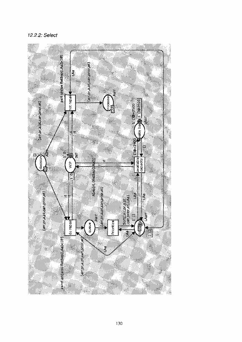
12.2.2: Select

130

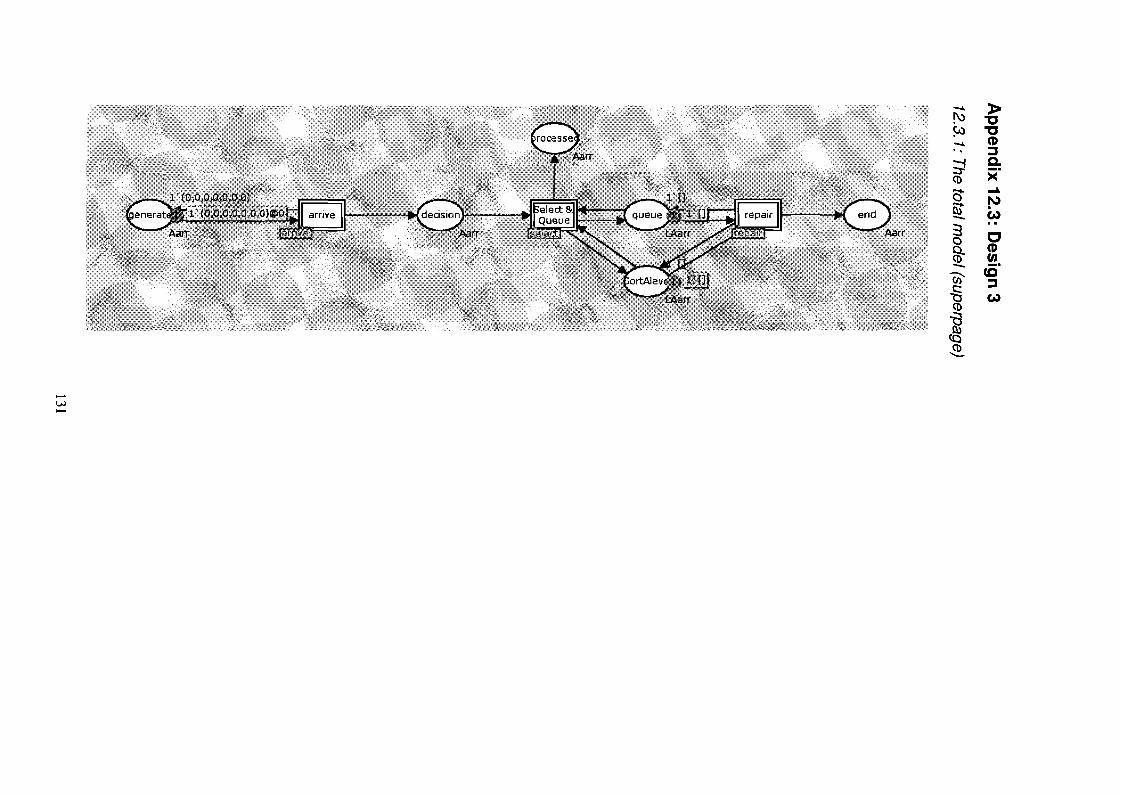
..... »!':> "C~ "C..... CD.. ::::J

~Q.

(J) ;<"8" ......iii !':»- Cot)

:3 c0

~CD(J)- cC"Ci)'

-§::::J

(J)Cot)

-a

......

~

UJ

~

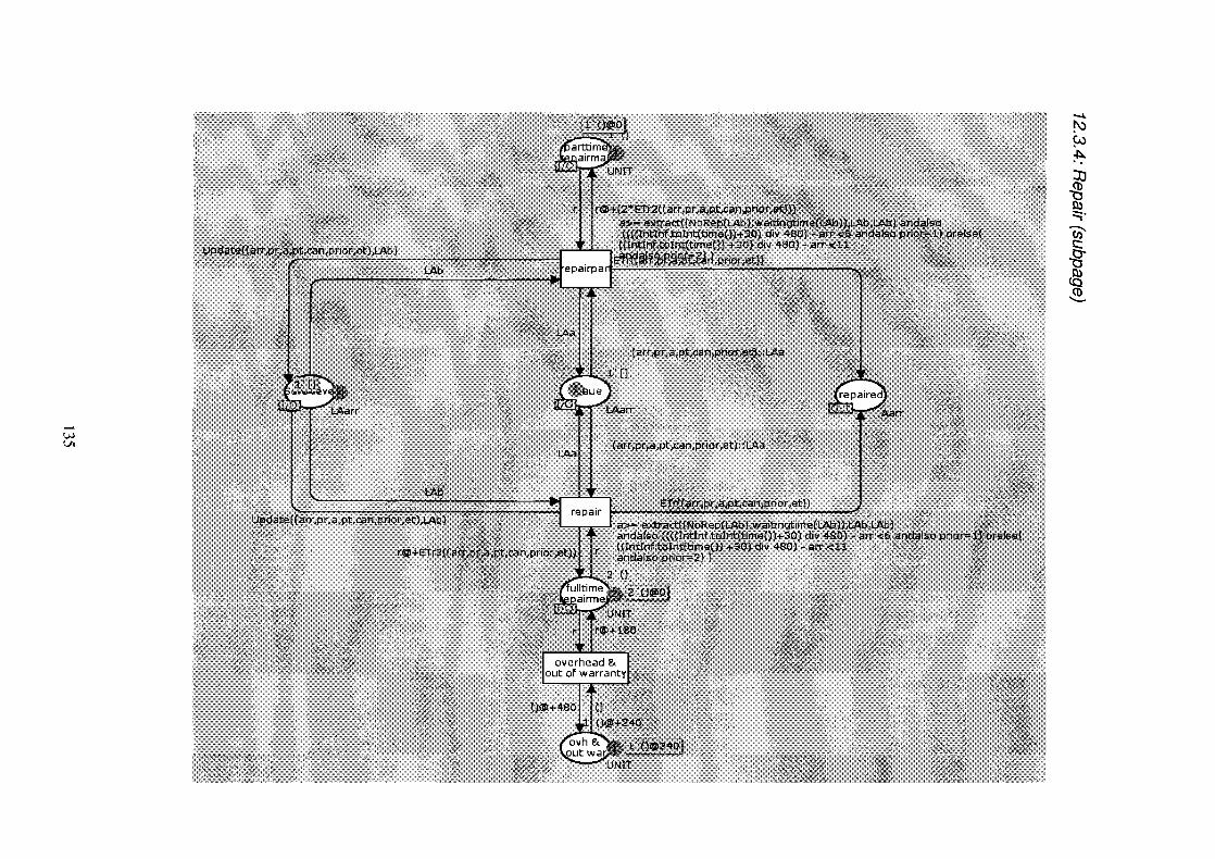
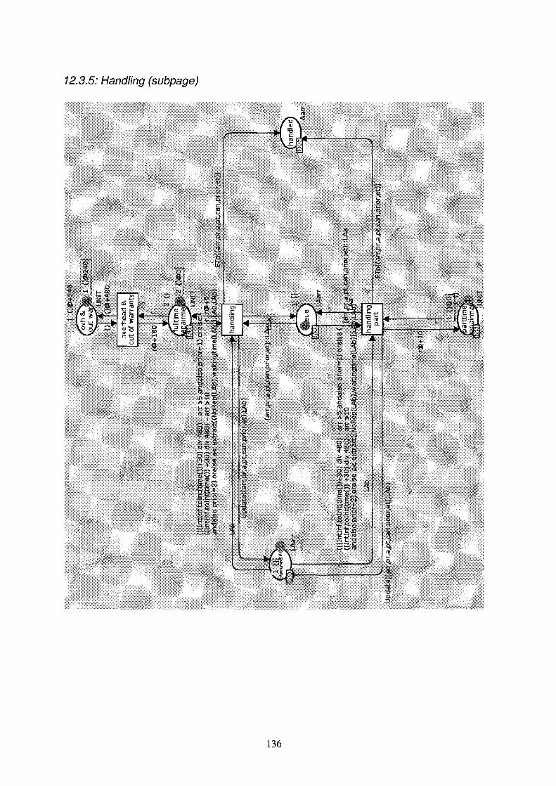
12.3.5: Handling (subpage)

136

Appendix 12.4: Declarations

12.4. 1: Declarations 1

'ffDeciarationsStandarddedarations

"calset arrtime = INT timedi"calset price = INT;"calset A= INT timed;"co!set processingtime 1" INTi'ffcoIset cannibalization = INT;'ffcOIset priority = INTi..... colset endtime = INT;"colset day"'INT;..... var day:day;." colset dayvalue = INT;"calset daydayvalue ",product day • dayvaluei"colset wvar'" product INT • INn"var dt: INT;"calset Aarr ",;product arrtime· price

A2processirjgtime • canqipalizationpriOrity • endtime timed;

"colset LAart = list Aarr;"var arr: arrtimei"var pr: price;"var a: Ai"vat pt: processingtime;"wit dv: dayvatue;Tvar can: cannibalization;"var fw: INTi"var wk: INTi

prior: I~lJ..... var at: eqdtimei"var LAa :LAarr;"vafLAb: LAarri"fun>AT(a) =(Intlnf.tdlnt(timeOD"fun renewdav(a,b)" if a""l then

else if a=3 then (4,125) else if a'" then (5,85) else (1,"fun Pric:e(a,b,c,d,e,f,g) '" if discrete(0,19) = 19 then (a,rou al(lOOO.0,250.0»,c,discrete(15,25

else if discrete(0,19»14 then (a,round(nOfrt:ial(175,0,25.0)), te 2Si45),el,g) else if discrete(O,19) >8 thenround(nOfm~!(75.0,8.33));C, ),e,f,g) else if discrete(O,19»2then (a,roqqg(normal .5,4.17 e(20,40),e,f,g) else (a,ro4nd(normal(.17)),c,discrete(15,25),e,f,g);

.,fyn reneW4(a,b) 1 then (else ifa""2 thenelse lfa=2 thenelse if a=4 then ,1015)else if a""5 then (6,96)else if a=6 then (7,100)else if a=7 then (8,111)else if a""8 tt)en (9,95)el~e if a=9~hen (10, 90~else if a=10 then (11,86)els~Jf a=llthen (12,69)else if a""12 then (13,115) elSe

"fun cannibal(a)'" i(discrete (0"fun priority(a) =if discrete{O,9)<"var rl: INT;"fun A(a,b,c,d,e,f,g) =(a,b,b·10 div d,d, el,g);

137

12.4.2: Declarations 2

."var r; UNIT;"fun Sort((a,b,c,d,e,f,g),[]) == [(a,b,c,d,e,f,g)] I

Sort((a,b,cid,e,f,g),(h,i,Lk,I,m,n): :t) == if f=m andalso a<hthen (a,b,c,d,e,f,9):: ((h,i,j,k,l,m,n): :t)els~jf f<m andalSo a - h <= 1 then (a,b,c,d,e,f,g):: ((h,i,J,k,I,m,n): :t) else(hiiiJik,I,m,n): :Sbrt((a,b,c,d,e,f,Q),t);

"fun ET(a,b,c,d,e,f,g) = if e=O then (a,b,c,d,e,fi'((IntInf.tolnt· m+r8~'Jd(norm al(d),S.O)))) div 4Bg~. ~Ise (a,b,c,d,e,f,W f.totht(timem

round(nor .. }i ),S.O))+ 1S) )diI/4BO) ,;Sortfive((a,b,c,d,e,f,g)'Dl=:=: [(a,b,c,d,e,f,g)] I

50rtfi'!l~(..(~,b,c,d,e,f,g),(h,i,j,k,l;m,.I1): :t) = if f=m aridalsoa<;hthen (a,b,c,d,e,f,g): :~Ih,i,Jlk,l,m,n)::t)else if f<m andalso q - h <=5 then (a,b,c,d,e,f,g):: ((h,i,J,k,l,m,n): :t) else(h,i,j,k,I,mf~~J:Sort((a,b,c,d,e,f,g)f~l;

Tfun ET2(a,b,c,d,e,f,g) = if e=O thenround(normal(rea/(d),S.O)) elserynd(l'lormal(r~al(d),5.0))+ 15 ,;

n Abep(a,b) = if a=O then 35 else if b - 190 ;> 60 then a+6else if b-190>SOthen a+S else if b-190;>40 then a+4 else if b-190>30 then a+:3.~Ise if b~+~Q;>20 then a+2 else if b-190>10 then a+1 else if 190-b>60 13-6else if 190"b>50 thena+5.else if 190-b>40 th.en a-4 else if 190-b> 30 then a-3else if 190-b>20 then a'-2 else jf b-190<10 aridalso 190-b a else a-;l;

IJJoofungetBep

138

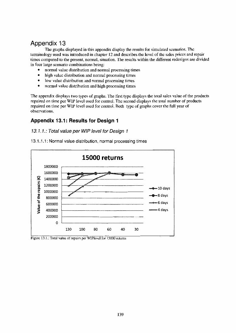
Appendix 13The graphs displayed in this appendix display the results for simulated scenarios. The

terminology used was introduced in chapter 12 and describes the level of the sales prices and repairtimes compared to the present, normal, situation. The results within the different redesigns are dividedin four large scenario combinations being:

• normal value distribution and normal processing times• high value distribution and normal processing times• low value distribution and normal processing times• normal value distribution and high processing times

The appendix displays two types of graphs. The first type displays the total sales value of the productsrepaired on time per WIP level used for control. The second displays the total number of productsrepaired on time per WIP level used for control. Both type of graphs cover the full year ofobservations.

Appendix 13.1: Results for Design 1

13. 1. 1.: Total value per WIP level for Design 1

13.1.1.1 : Normal value distribution, normal processing times

15000 returns1800000

1600000

2: 1400000III...

1200000'iiic.QI 1000000...QI.c 800000........0 600000QI

2400000III

>200000

0

""""10 days

-e-8days

~6days

............4 days

130 100 80 60 40 30

Figure 13.1.: Total value of repairs per WIPlevel for 15000 returns

139

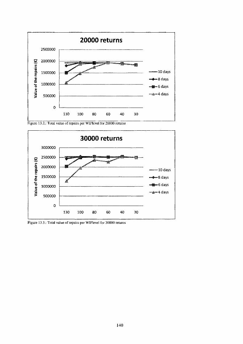
2500000

2: 2000000III...'iiiDo 1500000QI...QI

.=....1000000-0

QI:::JIII 500000>

0

20000 returns

-10 days

-+-8 days

"""6 days

~4days

130 100 80 60 40 30

Figure 13.2.: Total value of repairs per WIPlevel for 20000 returns

30000 returns3000000

2: 2500000III...

2000000'iiiDoQI...QI 1500000.=....-0 1000000QI:::J"iii> 500000

0

-10 days

-+-8 days

"""6 days

~4days

130 100 80 60 40 30

Figure 13.3.: Total value of repairs per WIPlevel for 30000 returns

140

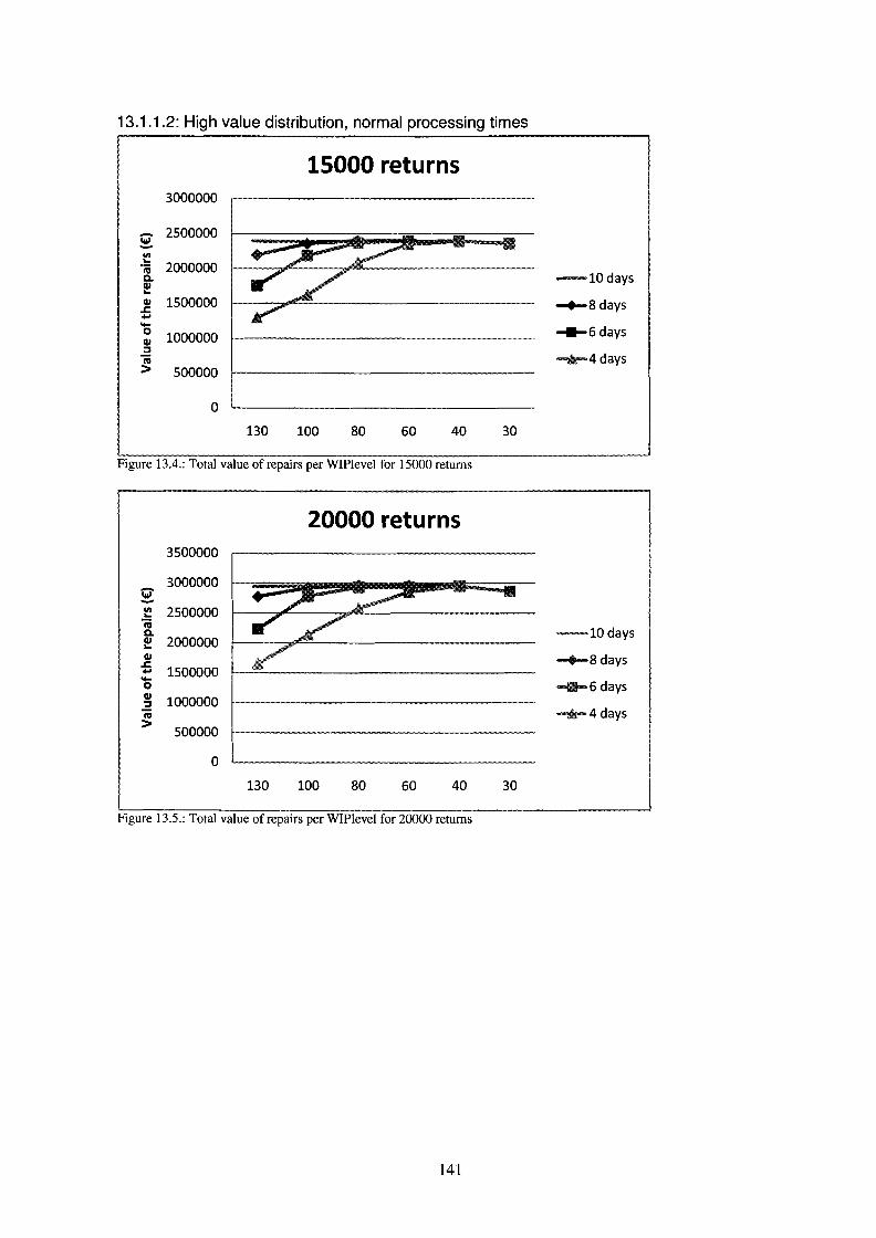
13.1.1.2: High value distribution, normal processing times

15000 returns3000000

~2500000

'"... 2000000'iiiDoQl...Ql 1500000.!:..-0 1000000Ql~

"'iii> 500000

0

-10 days

~8days

_6 days

""""4 days

130 100 80 60 40 30

Figure 13.4.: Total value of repairs per WIPlevel for 15000 returns

20000 returns3500000

3000000~'" 2500000...'iiiDoQl 2000000...Ql

.!:1500000..-0

Ql 1000000~

"'iii> 500000

0

-10 days

~8days

_6 days

""""4 days

130 100 80 60 40 30

Figure 13.5.: Total value of repairs per WIPlevel for 20000 returns

141

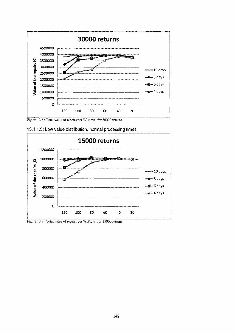
30000 returns4500000

4000000

2: 3500000~.; 3000000Q.

~ 2500000CIl

£ 2000000....~ 1500000::::Iia 1000000>

500000

o

-10 days

.........Sdays

__6 days

""""4 days

130 100 so 60 40 30

Figure 13.6.: Total value of repairs per WIPlevel for 30000 returns

13.1.1.3: Low value distribution, normal processing times

15000 returns1200000

2: 1000000III...

SOOOOO.;Q.CIl...CIl 600000..c........0 400000CIl::::Iia> 200000

0

-10 days

.........Sdays

__6 days

""""4 days

130 100 so 60 40 30

Figure 13.7.: Total value of repairs per WIPlevel for 15000 returns

142

1400000

12000002:'" 1000000...

"iiiQ.CII 800000...CII

.t:.600000........

0CII 400000:::J'iii> 200000

0

20000 returns

-10 days

......-8 days

""6 days

""""4 days

130 100 80 60 40 30

Figure 13.8.: Total value of repairs per WIPlevel for 20000 returns

30000 returns1800000

1600000

2: 1400000'"·i 1200000Q.

! 1000000CII

£ 800000'0CII 600000:::J

~ 400000

200000

o

-10 days

......-8 days

_6 days

........4 days

130 100 80 60 40 30

Figure 13.9.: Total value of repairs per WIPlevel for 30000 returns

143

13.1.1.4: Normal value distribution, low processing times

15000 returns1800000

1600000

2: 1400000III...

1200000'n;Q.QI 1000000...QI~ 800000........0 600000QI:s"'iii 400000>

200000

0

-10 days

........8 days

.......6 days

~4days

130 100 80 60 40 30

Figure 13.10.: Total value of repairs per WIPlevel for 15000 returns

20000 returns2500000

2: 2000000III...'n;Q. 1500000QI...QI~....

1000000....0QI:s"'iii 500000>

o

-10 days

""""8 days

.......6 days

~4days

130 100 80 60 40 30

Figure 13.11.: Total value of repairs per WIPlevel for 20000 returns

144

30000 returns3000000

2: 2500000III...

2000000'iiia.eu...eu 1500000.c........0 1000000eu2III> 500000

0

-10 days

...-8 days

........6 days

~4days

130 100 80 60 40 30

Figure 13.12.: Total value ofrepairs per WIPlevel for 30000 returns

13.1.2: Number of repairs per WIPlevel

13.1.2.1.: Normal value distribution, normal processing times

Repairs per WIP level

8600

8400

8200

.l!l 8000u

-6 7800~a. 7600

7400

7200

7000

...-15000

""""20000

~30000

130 100 80 60 40 30

Fig 13.13. Nonnal value, nonnal processing times: total number of repairs per WIPlevel,

145

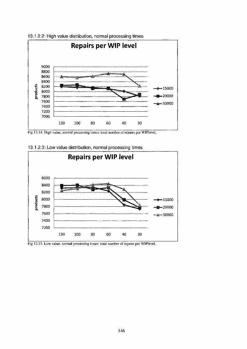
13.1.2.2: High value distribution, normal processing times

Repairs per WIP level

9000880086008400

-e 8200.g 80002 7800Q.

7600740072007000

-....15000

""'-20000

......... 30000

130 100 80 60 40 30

Fig 13.14. High value, normal processing times: total number of repairs per WIPlevel,

13.1.2.3: Low value distribution, normal processing times

Repairs per WIP level

8600

8400

8200IIIg 8000

"1::Je 7800Q.

7600

7400

7200

-....15000

""'-20000

......... 30000

130 100 80 60 40 30

Fig 13.15. Low value, normal processing times: total number of repairs per WIPlevel,

146

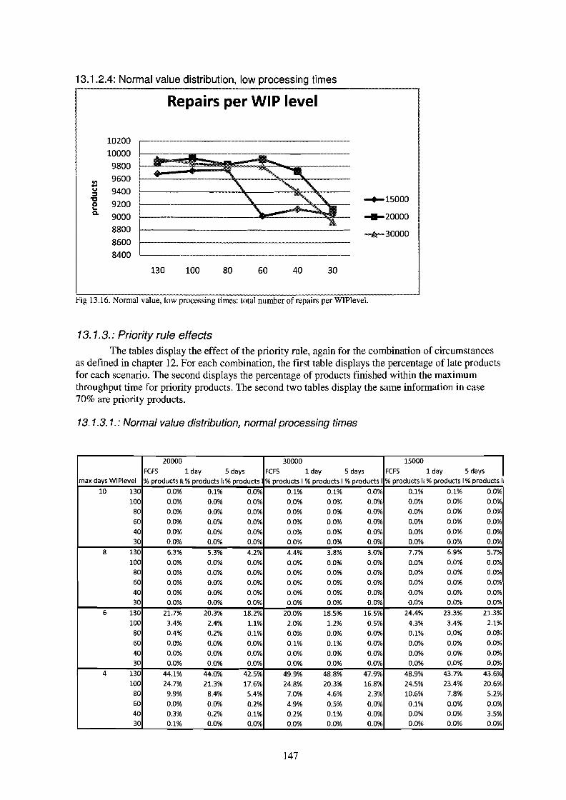
13.1 .2.4: Normal value distribution, low processing times

Repairs per WIP level

III....u:::s~o'­0..

10200

10000

9800

9600

9400

9200

9000

8800

8600

8400

-+-15000

~20000

........30000

130 100 80 60 40 30

Fig 13.16. Nonnal value, low processing times: total number of repairs per WIPlevel,

13.1.3.: Priority rule effects

The tables display the effect of the priority rule, again for the combination of circumstancesas defined in chapter 12. For each combination, the first table displays the percentage of late productsfor each scenario. The second displays the percentage of products finished within the maximumthroughput time for priority products. The second two tables display the same information in case70% are priority products.

13.1.3.1.: Normal value distribution, normal processing times

20000 30000 150001FCFS 1 day 5 days FCFS 1 day 5 days FCFS 1 day 5 days

max days WIPlevel % products I, % products I; % products I % products I% products I% products I % products I, % products I% products I;

10 130 0.0% 0.1% 0.0% 0.1% 0.1% 0.0% 0.1% 0.1% 0.0%

100 0.0% 0.0% 0.0% 0.0% 0.0% 0.0% 0.0% 0.0% 0.0%

80 0.0% 0.0% 0.0% 0.0% 0.0% 0.0% 0.0% 0.0% 0.0%

60 0.0% 0.0% 0.0% 0.0% 0.0% 0.0% 0.0% 0.0% 0.0%

40 0.0% 0.0% 0.0% 0.0% 0.0% 0.0% 0.0% 0.0% 0.0%30 0.0% 0.0% 0.0% 0.0% 0.0% 0.0% 0.0% 0.0% 0.0%

8 130 6.3% 5.3% 4.2% 4.4% 3.8% 3.0% 7.7% 6.9% 5.7%

100 0.0% 0.0% 0.0% 0.0% 0.0% 0.0% 0.0% 0.0% 0.0%80 0.0% 0.0% 0.0% 0.0% 0.0% 0.0% 0.0% 0.0% 0.0%

60 0.0% 0.0% 0.0% 0.0% 0.0% 0.0% 0.0% 0.0% 0.0%

40 0.0% 0.0% 0.0% 0.0% 0.0% 0.0% 0.0% 0.0% 0.0%30 0.0% 0.0% 0.0% 0.0% 0.0% 0.0% 0.0% 0.0% 0.0%

6 130 21.7% 20.3% 18.2% 20.0% 18.5% 16.5% 24.4% 23.3% 21.3%

100 3.4% 2.4% 1.1% 2.0% 1.2% 0.5% 4.3% 3.4% 2.1%

80 0.4% 0.2% 0.1% 0.0% 0.0% 0.0% 0.1% 0.0% 0.0%

60 0.0% 0.0% 0.0% 0.1% 0.1% 0.0% 0.0% 0.0% 0.0%

40 0.0% 0.0% 0.0% 0.0% 0.0% 0.0% 0.0% 0.0% 0.0%

30 0.0% 0.0% 0.0% 0.0% 0.0% 0.0% 0.0% 0.0% 0.0%

4 130 44.1% 44.0% 42.5% 49.9% 48.8% 47.9% 48.9% 43.7% 43.6%100 24.7% 21.3% 17.6% 24.8% 20.3% 16.8% 24.5% 23.4% 20.6%

80 9.9% 8.4% 5.4% 7.0% 4.6% 2.3% 10.6% 7.8% 5.2%60 0.0% 0.0% 0.2% 4.9% 0.5% 0.0% 0.1% 0.0% 0.0%40 0.3% 0.2% 0.1% 0.2% 0.1% 0.0% 0.0% 0.0% 3.5%30 0.1% 0.0% 0.0% 0.0% 0.0% 0.0% 0.0% 0.0% 0.0%

147

Table 13.1: Percentage of products late per WIP level, given priority and maximal throughput time, 90%

20000 30000 150001day 5 days IFCFS 1day 5 days FCFS 1day 5 days FCFS

max days WIPlevel % products ~ % products v% products % products \ % products \ % products % products ~ % products' % products v

10 130 100.0% 99.8% 97.2% 99.9% 99.8% 97.4% 99.9% 99.8% 96.8%

100 100.0% 100.0% 99.6% 100.0% 100.0% 99.8% 100.0% 100.0% 99.5%

80 100.0% 100.0% 100.0% 100.0% 100.0% 100.0% 100.0% 100.0% 100.0%60 100.0% 100.0% 100.0% 100.0% 100.0% 100.0% 100.0% 100.0% 100.0%40 100.0% 100.0% 100.0% 100.0% 100.0% 100.0% 100.0% 100.0% 100.0%30 100.0% 100.0% 100.0% 100.0% 100.0% 100.0% 100.0% 100.0% 100.0%

8 130 93.0% 92.9% 89.9% 95.1% 94.5% 89.8% 91.5% 91.0% 88.7%

100 100.0% 100.0% 94.7% 100.0% 100.0% 94.7% 100.0% 99.8% 94.5%

80 100.0% 100.0% 96.8% 100.0% 100.0% 97.1% 100.0% 100.0% 96.1%

60 100.0% 100.0% 99.1% 100.0% 100.0% 96.8% 100.0% 100.0% 99.1%40 100.0% 100.0% 97.2% 100.0% 100.0% 99.6% 100.0% 100.0% 100.0%30 100.0% 100.0% 100.0% 100.0% 100.0% 100.0% 100.0% 100.0% 100.0%

6 130 75.9% 75.4% 75.2% 77.7% 76.7% 77.0% 72.9% 72.4% 71.4%

100 96.2% 95.9% 91.0% 97.8% 97.2% 91.7% 95.3% 94.7% 89.9%

80 99.6% 99.4% 92.7% 100.0% 99.9% 92.5% 99.9% 99.6% 91.9%60 100.0% 100.0% 93.9% 99.9% 99.6% 92.3% 100.0% 100.0% 93.5%40 100.0% 100.0% 99.8% 100.0% 100.0% 94.5% 100.0% 100.0% 96.5%30 100.0% 100.0% 99.0% 100.0% 100.0% 97.8% 100.0% 100.0% 98.9%

4 130 51.3% 50.1% 54.6% 44.7% 44.0% 49.1% 55.6% 50.7% 53.2%

100 72.5% 73.0% 76.7% 74.2% 74.2% 77.9% 71.1% 70.8% 73.9%

80 89.1% 87.7% 87.9% 92.3% 91.7% 90.4% 88.2% 87.9% 87.5%

60 98.5% 97.4% 93.1% 89.1% 88.4% 88.5% 98.8% 97.5% 92.5%

40 99.7% 99.4% 96.3% 99.8% 99.0% 93.5% 100.0% 99.9% 95.3%30 99.9% 100.0% 98.2% 100.0% 100.0% 96.9% 100.0% 100.0% 98.0%

Table 13.2: Percentage of products wlthm x days per WIP level, gIven pnonty and maXImal throughput tIme, 90%

148

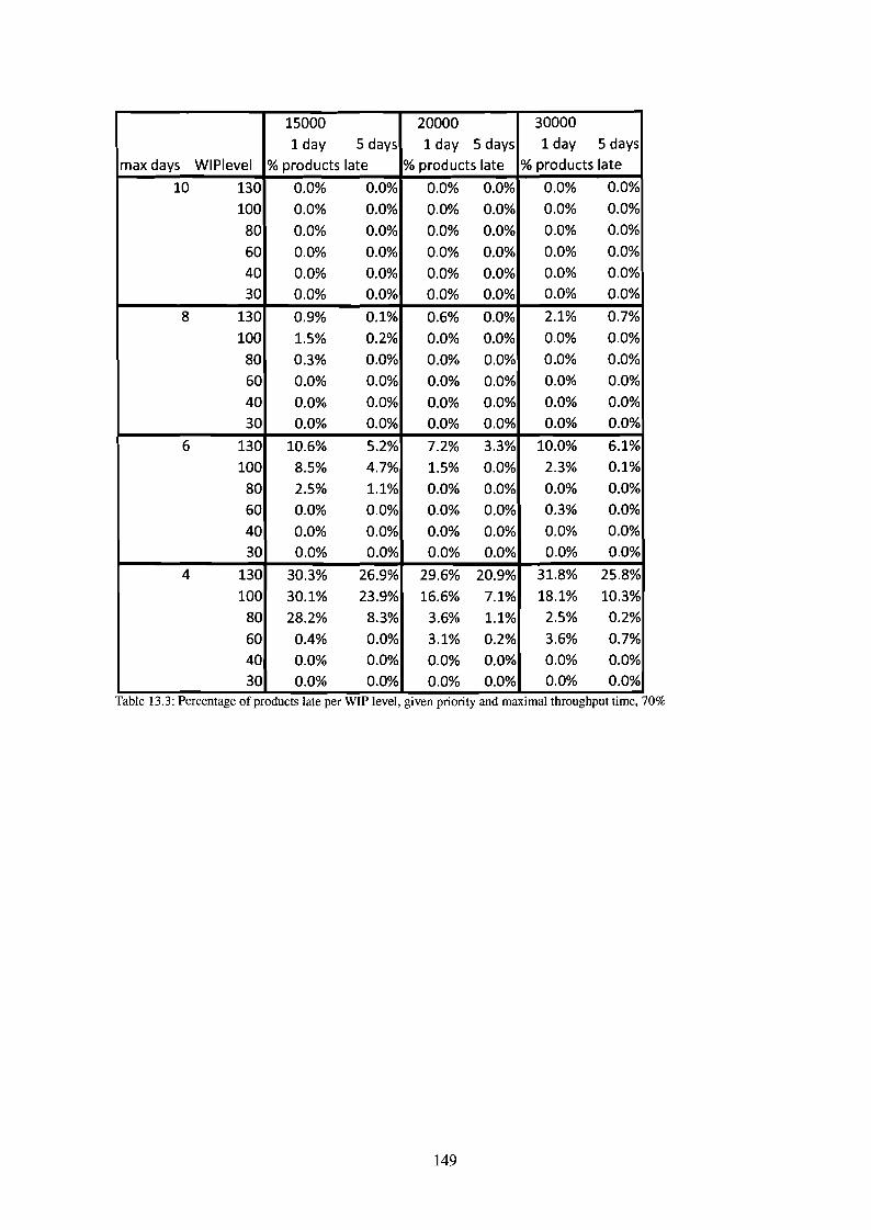
15000 20000 30000

1 day 5 days 1 day 5 days 1 day 5 days

max days WIPlevel % products late % products late % products late

10 130 0.0% 0.0% 0.0% 0.0% 0.0% 0.0%

100 0.0% 0.0% 0.0% 0.0% 0.0% 0.0%

80 0.0% 0.0% 0.0% 0.0% 0.0% 0.0%

60 0.0% 0.0% 0.0% 0.0% 0.0% 0.0%

40 0.0% 0.0% 0.0% 0.0% 0.0% 0.0%

30 0.0% 0.0% 0.0% 0.0% 0.0% 0.0%

8 130 0.9% 0.1% 0.6% 0.0% 2.1% 0.7%

100 1.5% 0.2% 0.0% 0.0% 0.0% 0.0%

80 0.3% 0.0% 0.0% 0.0% 0.0% 0.0%

60 0.0% 0.0% 0.0% 0.0% 0.0% 0.0%

40 0.0% 0.0% 0.0% 0.0% 0.0% 0.0%

30 0.0% 0.0% 0.0% 0.0% 0.0% 0.0%

6 130 10.6% 5.2% 7.2% 3.3% 10.0% 6.1%

100 8.5% 4.7% 1.5% 0.0% 2.3% 0.1%

80 2.5% 1.1% 0.0% 0.0% 0.0% 0.0%

60 0.0% 0.0% 0.0% 0.0% 0.3% 0.0%

40 0.0% 0.0% 0.0% 0.0% 0.0% 0.0%

30 0.0% 0.0% 0.0% 0.0% 0.0% 0.0%

4 130 30.3% 26.9% 29.6% 20.9% 31.8% 25.8%

100 30.1% 23.9% 16.6% 7.1% 18.1% 10.3%

80 28.2% 8.3% 3.6% 1.1% 2.5% 0.2%

60 0.4% 0.0% 3.1% 0.2% 3.6% 0.7%

40 0.0% 0.0% 0.0% 0.0% 0.0% 0.0%

30 0.0% 0.0% 0.0% 0.0% 0.0% 0.0%Table 13.3: Percentage of products late per WIP level, gIven pnonty and maxImal throughput time, 70%

149

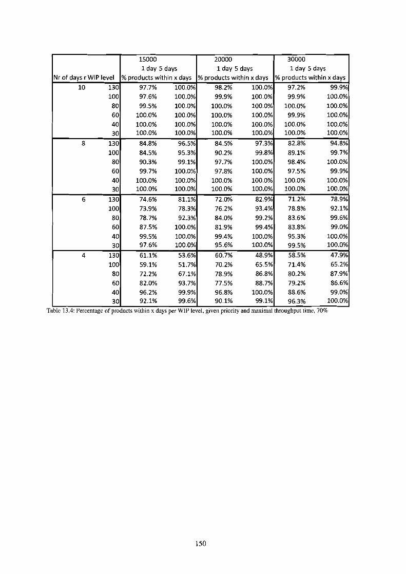
15000 20000 300001 day 5 days 1 day 5 days 1 day 5 days

Nr of days r WIP level % products within x days % products within x days % products within x days

10 130 97.7% 100.0% 98.2% 100.0% 97.2% 99.9%

100 97.6% 100.0% 99.9% 100.0% 99.9% 100.0%

80 99.5% 100.0% 100.0% 100.0% 100.0% 100.0%

60 100.0% 100.0% 100.0% 100.0% 99.9% 100.0%

40 100.0% 100.0% 100.0% 100.0% 100.0% 100.0%30 100.0% 100.0% 100.0% 100.0% 100.0% 100.0%

8 130 84.8% 96.5% 84.5% 97.3% 82.8% 94.8%

100 84.5% 95.3% 90.2% 99.8% 89.1% 99.7%

80 90.3% 99.1% 97.7% 100.0% 98.4% 100.0%

60 99.7% 100.0% 97.8% 100.0% 97.5% 99.9%

40 100.0% 100.0% 100.0% 100.0% 100.0% 100.0%30 100.0% 100.0% 100.0% 100.0% 100.0% 100.0%

6 130 74.6% 81.1% 72.0% 82.9% 71.2% 78.9%

100 73.9% 78.3% 76.2% 93.4% 78.8% 92.1%

80 78.7% 92.3% 84.0% 99.2% 83.6% 99.6%

60 87.5% 100.0% 81.9% 99.4% 83.8% 99.0%

40 99.5% 100.0% 99.4% 100.0% 95.3% 100.0%

30 97.6% 100.0% 95.6% 100.0% 99.5% 100.0%

4 130 61.1% 53.6% 60.7% 48.9% 58.5% 47.9%

100 59.1% 51.7% 70.2% 65.5% 71.4% 65.2%

80 72.2% 67.1% 78.9% 86.8% 80.2% 87.9%

60 82.0% 93.7% 77.5% 88.7% 79.2% 86.6%

40 96.2% 99.9% 96.8% 100.0% 88.6% 99.0%30 92.1% 99.6% 90.1% 99.1% 96.3% 100.0%

Table 13.4: Percentage of products wlthm x days per WIP level, given pnonty and maximal throughput time, 70%

150

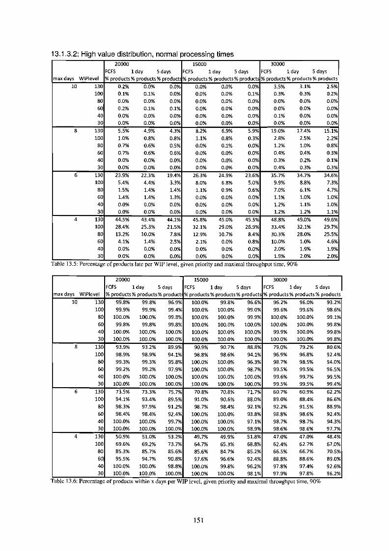
13.1.3.2: High value distribution, normal processing times20000 15000 30000 I

FCFS 1 day 5 days FCFS 1 day 5 days FCF5 1 day 5 daysmax days WIPlevel % products % products % product % products % products % products % products % products % products

10 130 0.2% 0.0% 0.0% 0.0% 0.0% 0.0% 3.5% 3.1% 2.5%100 0.1% 0.1% 0.0% 0.0% 0.0% 0.1% 0.3% 0.3% 0.2%

80 0.0% 0.0% 0.0% 0.0% 0.0% 0.0% 0.0% 0.0% 0.0%60 0.2% 0.1% 0.1% 0.0% 0.0% 0.0% 0.0% 0.0% 0.0%40 0.0% 0.0% 0.0% 0.0% 0.0% 0.0% 0.1% 0.0% 0.0%30 0.0% 0.0% 0.0% 0.0% 0.0% 0.0% 0.0% 0.0% 0.0%

8 130 5.5% 4.9% 4.3% 8.2% 6.9% 5.9% 19.0% 17.4% 15.1%100 1.0% 0.8% 0.8% 1.1% 0.8% 0.3% 2.8% 2.5% 2.2%80 0.7% 0.6% 0.5% 0.0% 0.1% 0.0% 1.2% 1.0% 0.8%

60 0.7% 0.6% 0.6% 0.0% 0.0% 0.0% 0.4% 0.4% 0.3%

40 0.0% 0.0% 0.0% 0.0% 0.0% 0.0% 0.3% 0.2% 0.1%30 0.0% 0.0% 0.0% 0.0% 0.0% 0.0% 0.4% 0.3% 0.3%

6 130 23.9% 22.3% 19.4% 26.3% 24.9% 23.6% 35.7% 34.7% 34.6%100 5.4% 4.4% 3.3% 8.0% 6.8% 5.0% 9.9% 8.8% 7.3%80 1.5% 1.4% 1.4% 1.1% 0.9% 0.6% 7.0% 6.1% 4.7%60 1.4% 1.4% 1.3% 0.0% 0.0% 0.0% 1.1% 1.0% 1.0%40 0.0% 0.0% 0.0% 0.0% 0.0% 0.0% 1.2% 1.1% 1.0%30 0.0% 0.0% 0.0% 0.0% 0.0% 0.0% 1.2% 1.2% 1.1%

4 130 44.5% 43.4% 44.1% 45.8% 45.0% 45.5% 48.8% 49.0% 49.6%100 28.4% 25.3% 21.5% 32.1% 29.0% 26.9% 33.4% 32.1% 29.7%

80 13.2% 10.0% 7.8% 12.9% 10.7% 8.4% 30.3% 28.0% 25.5%60 4.1% 1.4% 2.5% 2.1% 0.0% 0.8% 10.0% 1.0% 4.6%40 0.0% 0.0% 0.0% 0.0% 0.0% 0.0% 2.0% 1.9% 1.9%30 0.0% 0.0% 0.0% 0.0% 0.0% 0.0% 1.9% 2.0% 2.0%

Table 13.5: Percentage of products late per WIP level, given pnonty and maximal throughput time, 90%

max days WIPlevel

20000 15000 30000 IFCFS 1 day 5 days FCFS 1 day 5 days FCFS 1 day 5 days

% products % products % product % products % products % products % products % products % products

10 130

100

80

60

4030

8 130

100

80

6040

30

6 130

100

80

604030

4 130

10080

6040

30

99.8%

99.9%

100.0%

99.8%

100.0%100.0%

93.9%

98.9%99.3%

99.2%

100.0%100.0%

73.5%

94.1%

98.3%

98.4%

100.0%100.0%

50.9%

69.6%85.3%

95.5%

100.0%100.0%

99.8%

99.9%

100.0%

99.8%100.0%100.0%

93.2%

98.9%99.3%

99.2%

100.0%100.0%

73.3%

93.4%

97.9%

98.4%

100.0%100.0%

51.0%

69.2%85.7%

94.7%100.0%100.0%

96.9%

99.4%

99.8%

99.8%

100.0%100.0%

89.9%

94.1%

95.8%

97.9%

100.0%100.0%

75.7%

89.5%

91.2%92.4%

99.7%100.0%

53.2%

73.7%

85.6%

90.8%

98.8%100.0%

100.0%

100.0%

100.0%

100.0%

100.0%100.0%

90.9%

98.8%

100.0%100.0%

100.0%100.0%

70.8%

91.0%

98.7%

100.0%

100.0%100.0%

49.7%

64.7%

85.6%

97.6%

100.0%100.0%

99.8%

100.0%

100.0%

100.0%

100.0%100.0%

90.7%

98.6%

100.0%

100.0%

100.0%100.0%

70.8%

90.6%

98.4%

100.0%

100.0%100.0%

49.9%

65.3%84.7%

96.6%

99.8%100.0%

96.6%

99.0%

99.9%

100.0%

100.0%100.0%

88.8%

94.1%

96.3%98.7%

100.0%

100.0%

71.7%

88.0%

92.1%

93.8%

97.1%98.9%

51.8%

68.8%85.2%

92.4%

96.2%98.1%

96.2%

99.6%

100.0%

100.0%

99.9%100.0%

79.0%

96.9%98.7%

99.5%

99.6%99.5%

60.7%

89.0%

92.2%

98.8%

98.7%98.6%

47.0%

62.4%66.5%

88.8%97.8%97.9%

96.0%

99.6%

100.0%

100.0%

100.0%100.0%

79.2%

96.8%

98.5%

99.5%99.7%

99.5%

60.9%

88.4%

91.5%

98.6%

98.7%98.6%

47.0%

62.7%66.7%

88.6%

97.4%97.8%

93.2%

98.6%

99.1%

99.8%

99.8%99.8%

80.6%

92.4%

94.0%

96.5%

99.5%99.4%

62.2%

86.6%

88.9%

92.4%

94.3%97.7%

48.4%

67.0%

70.5%

89.0%

92.6%96.2%

Table 13.6: Percentage of products wlthm X days per WIP level, given pnonty and maXlmal throughput time, 90%

151

15000 20000 30000lday 5 days lday 5 days lday 5 days

Nr of days rWIP level % products late % products late % products late

10 130 0.0% 0.0% 0.1% 0.0% 0.4% 0.0%

100 0.0% 0.0% 0.0% 0.0% 1.6% 1.2%

80 0.0% 0.0% 0.0% 0.0% 0.5% 0.1%

60 0.0% 0.0% 0.0% 0.0% 0.0% 0.0%

40 0.0% 0.0% 0.0% 0.0% 0.0% 0.0%

30 0.0% 0.0% 0.0% 0.0% 0.0% 0.0%

8 130 1.6% 0.5% 4.3% 3.1% 7.4% 4.5%

100 0.1% 0.0% 0.5% 0.0% 3.3% 3.4%

80 0.0% 0.0% 0.0% 0.0% 1.8% 1.9%

60 0.0% 0.0% 0.0% 0.0% 0.2% 0.0%

40 0.0% 0.0% 0.0% 0.0% 0.0% 0.0%

30 0.0% 0.0% 0.0% 0.0% 0.0% 0.0%

6 130 10.2% 5.6% 15.4% 11.6% 22.4% 17.4%

100 2.4% 1.1% 7.3% 3.3% 4.9% 4.2%

80 0.0% 0.0% 0.0% 0.1% 2.9% 2.9%

60 0.0% 0.0% 0.0% 0.0% 0.9% 0.7%

40 0.0% 0.0% 0.0% 0.0% 0.0% 0.0%

30 0.0% 0.0% 0.0% 0.0% 0.0% 0.0%

4 130 29.5% 26.5% 33.4% 30.7% 37.0% 39.1%

100 17.9% 11.3% 24.7% 20.1% 15.3% 9.2%

80 8.4% 2.6% 4.6% 1.0% 5.9% 4.3%

60 0.4% 0.0% 0.8% 0.0% 5.2% 0.2%

40 0.4% 0.0% 0.0% 0.0% 0.0% 0.0%

30 0.1% 0.0% 0.0% 0.0% 0.0% 0.0%Table 13.7: Percentage of products late per WIP level, gIven pnonty and maxImal throughput tIme, 70%

152

15000 20000 30000

1 day 5 days 1 day 5 days 1 day 5 days

Nr of days r WIPlevel % products within x days % products within x days % products within x days

10 130 100.0% 97.5% 99.2% 95.2% 98.3% 92.6%

100 100.0% 99.5% 100.0% 98.2% 97.4% 97.8%

80 100.0% 100.0% 100.0% 100.0% 99.0% 98.8%

60 100.0% 100.0% 100.0% 100.0% 100.0% 99.6%

40 100.0% 100.0% 100.0% 100.0% 100.0% 100.0%

30 100.0% 100.0% 100.0% 100.0% 100.0% 100.0%

8 130 95.4% 84.8% 90.3% 83.7% 84.8% 83.2%

100 99.3% 90.5% 97.2% 86.4% 95.8% 92.2%

80 100.0% 94.8% 100.0% 97.2% 97.3% 97.4%

60 100.0% 99.5% 100.0% 99.3% 99.5% 97.1%

40 100.0% 99.7% 100.0% 100.0% 100.0% 100.0%

30 100.0% 99.9% 100.0% 100.0% 100.0% 100.0%

6 130 79.6% 77.2% 73.3% 66.3% 65.1% 61.4%

100 91.9% 80.4% 83.9% 78.1% 91.3% 81.2%

80 97.7% 82.6% 99.1% 84.6% 95.8% 86.1%

60 99.9% 89.6% 99.8% 86.4% 97.8% 85.2%

40 100.0% 89.5% 100.0% 99.2% 100.0% 96.6%

30 100.0% 98.7% 100.0% 95.8% 100.0% 99.8%

4 130 53.2% 65.4% 49.8% 59.6% 49.9% 56.3%

100 67.1% 78.5% 58.8% 76.2% 71.7% 78.5%

80 91.6% 79.7% 85.2% 80.8% 87.0% 81.5%

60 95.6% 84.6% 92.3% 81.7% 86.0% 80.8%

40 94.8% 85.2% 99.9% 96.5% 99.3% 90.4%

30 99.6% 96.2% 98.9% 89.4% 100.0% 98.7%

Table 13.8: Percentage of products wlthm x days per WIP level, gIven pnonty and maxImal throughput time, 70%

153

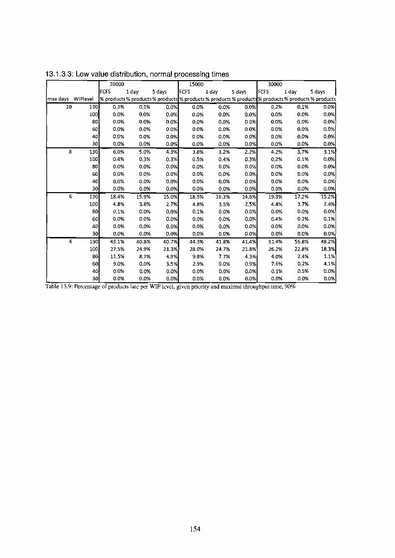
13.1.3.3: Low value distribution, normal processing times20000 15000 30000 IFCFS 1 day 5 days FCFS 1 day 5 days FCFS 1 day 5 days

max days WIPlevel % products % products % products % products % products % product % products % products % products

10 130 0.3% 0.1% 0.0% 0.0% 0.0% 0.0% 0.2% 0.1% 0.0%

100 0.0% 0.0% 0.0% 0.0% 0.0% 0.0% 0.0% 0.0% 0.0%

80 0.0% 0.0% 0.0% 0.0% 0.0% 0.0% 0.0% 0.0% 0.0%

60 0.0% 0.0% 0.0% 0.0% 0.0% 0.0% 0.0% 0.0% 0.0%

40 0.0% 0.0% 0.0% 0.0% 0.0% 0.0% 0.0% 0.0% 0.0%

30 0.0% 0.0% 0.0% 0.0% 0.0% 0.0% 0.0% 0.0% 0.0%

8 130 6.0% 5.0% 4.3% 3.8% 3.2% 2.2% 4.2% 3.7% 3.1%

100 0.4% 0.3% 0.3% 0.5% 0.4% 0.3% 0.2% 0.1% 0.0%

80 0.0% 0.0% 0.0% 0.0% 0.0% 0.0% 0.0% 0.0% 0.0%

60 0.0% 0.0% 0.0% 0.0% 0.0% 0.0% 0.0% 0.0% 0.0%

40 0.0% 0.0% 0.0% 0.0% 0.0% 0.0% 0.0% 0.0% 0.0%

30 0.0% 0.0% 0.0% 0.0% 0.0% 0.0% 0.0% 0.0% 0.0%

6 130 18.4% 15.9% 15.0% 18.5% 16.3% 14.6% 19.3% 17.2% 15.2%

100 4.8% 3.8% 2.7% 4.8% 3.5% 2.5% 4.4% 3.7% 2.4%

80 0.1% 0.0% 0.0% 0.1% 0.0% 0.0% 0.0% 0.0% 0.0%

60 0.0% 0.0% 0.0% 0.0% 0.0% 0.0% 0.4% 0.2% 0.1%

40 0.0% 0.0% 0.0% 0.0% 0.0% 0.0% 0.0% 0.0% 0.0%

30 0.0% 0.0% 0.0% 0.0% 0.0% 0.0% 0.0% 0.0% 0.0%

4 130 43.1% 40.8% 40.7% 44.3% 41.8% 41.4% 51.4% 56.8% 48.2%

100 27.5% 24.9% 21.3% 28.0% 24.7% 21.8% 26.2% 22.8% 18.3%

80 11.5% 8.7% 4.9% 9.8% 7.7% 4.3% 4.0% 2.4% 1.1%

60 9.0% 0.0% 3.5% 2.9% 0.0% 0.9% 7.6% 0.2% 4.1%

40 0.0% 0.0% 0.0% 0.0% 0.0% 0.0% 0.1% 0.5% 0.0%

30 0.0% 0.0% 0.0% 0.0% 0.0% 0.0% 0.0% 0.0% 0.0%

Table 13.9: Percentage of products late per WIP level, gIven poonty and maxlInal throughput tIme, 90%

154

20000 15000 30000 IFCFS 1 day 5 days FCFS 1 day 5 days FCFS 1 day 5 days

max days WIPlevel % products % products % products % products % products % product % products % products % products

10 130 99.7% 99.7% 97.4% 100.0% 100.0% 97.4% 99.8% 99.8% 97.3%100 100.0% 100.0% 99.4% 100.0% 100.0% 99.5% 100.0% 100.0% 99.4%

80 100.0% 100.0% 100.0% 100.0% 100.0% 100.0% 100.0% 100.0% 100.0%60 100.0% 100.0% 100.0% 100.0% 100.0% 100.0% 100.0% 100.0% 100.0%40 100.0% 100.0% 100.0% 100.0% 100.0% 100.0% 100.0% 100.0% 100.0%30 100.0% 100.0% 100.0% 100.0% 100.0% 100.0% 100.0% 100.0% 100.0%

8 130 93.3% 93.4% 89.6% 95.8% 95.4% 91.1% 95.4% 94.8% 89.3%100 99.6% 99.4% 94.2% 99.5% 99.4% 94.3% 99.8% 99.6% 94.8%80 100.0% 100.0% 96.1% 100.0% 100.0% 96.5% 100.0% 100.0% 97.8%60 100.0% 100.0% 96.6% 100.0% 100.0% 98.4% 100.0% 100.0% 97.1%40 100.0% 100.0% 100.0% 100.0% 100.0% 100.0% 100.0% 100.0% 99.9%30 100.0% 100.0% 100.0% 100.0% 100.0% 100.0% 100.0% 100.0% 100.0%

6 130 79.6% 80.2% 78.9% 79.5% 79.5% 79.1% 78.6% 78.3% 78.0%100 94.7% 94.1% 90.1% 94.7% 94.3% 89.9% 95.1% 94.4% 89.7%80 99.8% 99.5% 92.7% 99.9% 99.7% 92.4% 100.0% 99.9% 91.9%60 100.0% 99.7% 92.4% 100.0% 100.0% 93.3% 99.6% 99.4% 92.0%40 100.0% 100.0% 98.3% 100.0% 100.0% 97.5% 100.0% 100.0% 95.5%30 100.0% 100.0% 96.4% 100.0% 100.0% 98.9% 100.0% 100.0% 99.0%

4 130 52.4% 53.1% 56.3% 50.9% 51.7% 55.4% 43.3% 50.8% 48.7%100 69.6% 69.5% 74.0% 69.4% 69.6% 73.3% 71.2% 71.4% 76.0%

80 87.1% 86.8% 88.6% 89.1% 88.0% 88.8% 95.5% 94.2% 90.6%60 90.0% 89.2% 89.4% 96.8% 95.3% 92.0% 91.6% 90.0% 88.3%40 100.0% 100.0% 97.1% 100.0% 100.0% 96.3% 99.9% 100.0% 94.5%30 100.0% 100.0% 95.1% 100.0% 100.0% 98.0% 100.0% 100.0% 98.2%

Table 13.10: Percentage of products within x days per WIP level, given priority and maximal throughput time,90%

155

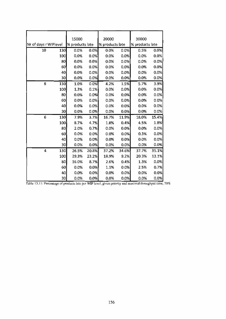
15000 20000 30000

Nr of days r WIPlevel % products late % products late % products late

10 130 0.0% 0.0% 0.0% 0.0% 0.5% 0.0%

100 0.0% 0.0% 0.0% 0.0% 0.0% 0.0%

80 0.0% 0.0% 0.0% 0.0% 0.0% 0.0%

60 0.0% 0.0% 0.0% 0.0% 0.0% 0.0%

40 0.0% 0.0% 0.0% 0.0% 0.0% 0.0%

30 0.0% 0.0% 0.0% 0.0% 0.0% 0.0%

8 130 1.0% 0.0% 4.2% 1.5% 5.7% 3.9%

100 1.3% 0.1% 0.0% 0.0% 0.0% 0.0%

80 0.0% 0.0% 0.0% 0.0% 0.0% 0.0%

60 0.0% 0.0% 0.0% 0.0% 0.0% 0.0%

40 0.0% 0.0% 0.0% 0.0% 0.0% 0.0%

30 0.0% 0.0% 0.0% 0.0% 0.0% 0.0%

6 130 7.9% 3.7% 16.7% 11.9% 18.0% 15.4%

100 8.7% 4.7% 1.8% 0.4% 4.5% 1.8%

80 2.0% 0.7% 0.0% 0.0% 0.0% 0.0%

60 0.0% 0.0% 0.0% 0.0% 0.3% 0.0%

40 0.0% 0.0% 0.0% 0.0% 0.0% 0.0%

30 0.0% 0.0% 0.0% 0.0% 0.0% 0.0%

4 130 26.5% 20.8% 37.2% 34.6% 37.7% 35.1%

100 29.3% 23.2% 18.9% 9.2% 20.3% 13.1%

80 16.0% 8.7% 2.6% 0.4% 1.3% 0.0%

60 0.0% 0.0% 1.1% 0.0% 2.5% 0.7%

40 0.0% 0.0% 0.0% 0.0% 0.0% 0.0%

30 0.0% 0.0% 0.0% 0.0% 0.0% 0.0%Table 13.11: Percentage of products late per WIP level, glven pnonty and maximal throughput tIme, 70%

156

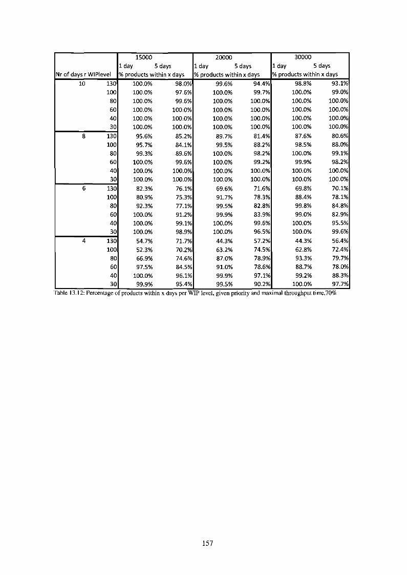
15000 20000 300001 day 5 days 1 day 5 days 1 day 5 days

Nr of days r WIPlevel % products within x days % products within x days % products within x days

10 130 100.0% 98.0% 99.6% 94.4% 98.8% 93.1%

100 100.0% 97.6% 100.0% 99.7% 100.0% 99.0%

80 100.0% 99.6% 100.0% 100.0% 100.0% 100.0%

60 100.0% 100.0% 100.0% 100.0% 100.0% 100.0%

40 100.0% 100.0% 100.0% 100.0% 100.0% 100.0%

30 100.0% 100.0% 100.0% 100.0% 100.0% 100.0%

8 130 95.6% 85.2% 89.7% 81.4% 87.6% 80.6%

100 95.7% 84.1% 99.5% 88.2% 98.5% 88.0%

80 99.3% 89.6% 100.0% 98.2% 100.0% 99.1%

60 100.0% 99.6% 100.0% 99.2% 99.9% 98.2%

40 100.0% 100.0% 100.0% 100.0% 100.0% 100.0%

30 100.0% 100.0% 100.0% 100.0% 100.0% 100.0%

6 130 82.3% 76.1% 69.6% 71.6% 69.8% 70.1%

100 80.9% 75.3% 91.7% 78.3% 88.4% 78.1%

80 92.3% 77.1% 99.5% 82.8% 99.8% 84.8%

60 100.0% 91.2% 99.9% 83.9% 99.0% 82.9%

40 100.0% 99.1% 100.0% 99.6% 100.0% 95.5%

30 100.0% 98.9% 100.0% 96.5% 100.0% 99.6%

4 130 54.7% 71.7% 44.3% 57.2% 44.3% 56.4%

100 52.3% 70.2% 63.2% 74.5% 62.8% 72.4%

80 66.9% 74.6% 87.0% 78.9% 93.3% 79.7%

60 97.5% 84.5% 91.0% 78.6% 88.7% 78.0%

40 100.0% 96.1% 99.9% 97.1% 99.2% 88.3%

30 99.9% 95.4% 99.5% 90.2% 100.0% 97.7%

Table 13.12: Percentage of products wIthm x days per WIP level, gIven priority and maximal throughput tIme,70%

157

13.1.3.4: Normal value distribution, low processing times

max days WIPlevel

10 130

10080604030

8 130

10080604030

6 130100

80604030

4 130

10080604030

20000 15000 30000 IFCFS 1 day 5 days FCFS 1 day 5 days FCFS 1 day 5 days% products % products % product % products % products % products % products % products % products

0.0% 0.0% 0.1% 0.0% 0.0% 0.0% 0.1% 0.1% 0.0%0.0% 0.0% 0.0% 0.0% 0.0% 0.0% 0.0% 0.0% 0.0%

0.0% 0.0% 0.0% 0.0% 0.0% 0.0% 0.0% 0.0% 0.0%0.0% 0.0% 0.0% 0.0% 0.0% 0.0% 0.0% 0.0% 0.0%0.0% 0.0% 0.0% 0.0% 0.0% 0.0% 0.0% 0.0% 0.0%0.0% 0.0% 0.0% 0.0% 0.0% 0.0% 0.0% 0.0% 0.0%

1.9% 1.4% 0.9% 1.9% 1.4% 0.9% 5.6% 4.6% 3.5%0.2% 0.1% 0.0% 0.1% 0.1% 0.0% 0.0% 0.0% 0.0%0.0% 0.0% 0.0% 0.0% 0.0% 0.0% 0.0% 0.0% 0.0%0.0% 0.0% 0.0% 0.0% 0.0% 0.0% 0.0% 0.0% 0.0%0.0% 0.0% 0.0% 0.0% 0.0% 0.0% 0.0% 0.0% 0.0%0.0% 0.0% 0.0% 0.0% 0.0% 0.0% 0.0% 0.0% 0.0%

12.4% 10.6% 8.5% 11.3% 10.3% 8.4% 20.3% 18.9% 17.0%3.6% 2.8% 1.8% 2.0% 1.5% 1.0% 3.0% 2.4% 1.3%0.0% 0.0% 0.0% 0.0% 0.0% 0.0% 0.1% 0.0% 0.0%0.0% 0.0% 0.0% 0.0% 0.0% 0.0% 0.0% 0.0% 0.0%0.0% 0.0% 0.0% 0.0% 0.0% 0.0% 0.0% 0.0% 0.0%0.0% 0.0% 0.0% 0.0% 0.0% 0.0% 0.0% 0.0% 0.0%

38.3% 36.9% 35.8% 36.3% 34.9% 32.7% 42.4% 40.9% 41.9%25.6% 24.0% 19.9% 14.6% 13.1% 10.1% 20.2% 17.4% 14.7%

1.5% 1.0% 0.3% 2.8% 1.7% 0.9% 1.6% 1.2% 0.6%1.2% 0.0% 0.2% 0.2% 0.0% 0.0% 4.0% 0.0% 2.2%0.0% 0.0% 0.0% 0.0% 0.0% 0.0% 0.2% 0.1% 0.0%0.0% 0.0% 0.0% 0.0% 0.0% 0.0% 0.0% 0.0% 0.0%

Table 13.13: Percentage of products late per WIP level, gIven pnonty and maJumal throughput tIme, 90%

158

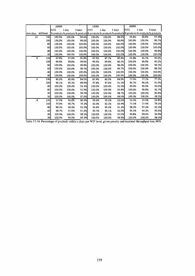
20000 15000 30000 1FCFS 1 day 5 days FCFS 1 day 5 days FCFS 1 day 5 days

max days WIPlevel % products % products % product % products % products % products % products % products % products

10 130 100.0% 100.0% 98.4% 100.0% 100.0% 98.6% 99.8% 99.8% 97.3%

100 100.0% 100.0% 99.6% 100.0% 100.0% 99.8% 100.0% 100.0% 99.7%

80 100.0% 100.0% 100.0% 100.0% 100.0% 100.0% 100.0% 100.0% 100.0%

60 100.0% 100.0% 100.0% 100.0% 100.0% 100.0% 100.0% 100.0% 100.0%

40 100.0% 100.0% 100.0% 100.0% 100.0% 100.0% 100.0% 100.0% 99.8%

30 100.0% 100.0% 100.0% 100.0% 100.0% 100.0% 100.0% 100.0% 100.0%

8 130 97.9% 97.9% 92.8% 97.9% 97.7% 93.4% 93.8% 93.7% 90.6%

100 99.8% 99.8% 94.5% 99.9% 99.8% 96.1% 100.0% 99.9% 95.2%

80 100.0% 100.0% 98.8% 100.0% 100.0% 98.3% 100.0% 100.0% 99.1%

60 100.0% 100.0% 98.7% 100.0% 100.0% 99.7% 100.0% 100.0% 98.1%

40 100.0% 100.0% 100.0% 100.0% 100.0% 100.0% 100.0% 100.0% 100.0%

30 100.0% 100.0% 100.0% 100.0% 100.0% 100.0% 100.0% 100.0% 100.0%

6 130 86.3% 85.9% 84.5% 87.4% 86.5% 84.9% 77.5% 77.1% 77.2%

100 96.1% 95.3% 89.9% 97.8% 97.6% 91.2% 96.7% 96.2% 91.0%

80 100.0% 100.0% 93.3% 100.0% 100.0% 92.5% 99.9% 99.9% 93.5%

60 100.0% 100.0% 92.9% 100.0% 100.0% 94.8% 100.0% 99.8% 92.7%

40 100.0% 100.0% 99.4% 100.0% 100.0% 98.7% 100.0% 100.0% 95.9%30 100.0% 100.0% 97.6% 100.0% 100.0% 99.5% 100.0% 100.0% 99.2%

4 130 57.5% 56.8% 60.3% 59.6% 59.2% 63.6% 53.2% 53.4% 54.8%

100 70.9% 69.7% 74.2% 82.6% 82.2% 83.4% 77.5% 77.4% 79.2%

80 98.3% 96.9% 92.3% 96.9% 95.4% 91.2% 98.2% 97.2% 92.3%

60 98.7% 97.0% 91.9% 99.7% 99.1% 93.9% 95.5% 94.3% 90.4%

40 100.0% 100.0% 98.5% 100.0% 100.0% 97.5% 99.8% 99.4% 94.9%30 100.0% 99.9% 96.3% 100.0% 100.0% 98.9% 100.0% 100.0% 98.3%

Table 13.14: Percentage of products wlthm x days per WIP level, gIven pnonty and maxImal throughput tIme,90%

159

15000 20000 30000

1 day 5 days 1 day 5 days 1 day 5 days

Nr of days IWIPlevel: % products late % products late % products late

10 130 0.0% 0.0% 0.0% 0.0% 0.0% 0.0%

100 0.0% 0.0% 0.0% 0.0% 0.0% 0.0%

80 0.0% 0.0% 0.0% 0.0% 0.0% 0.0%

60 0.0% 0.0% 0.0% 0.0% 0.0% 0.0%

40 0.0% 0.0% 0.0% 0.0% 0.0% 0.0%

30 0.0% 0.0% 0.0% 0.0% 0.0% 0.0%

8 130 0.7% 0.2% 0.3% 0.0% 1.5% 0.7%

100 0.0% 0.0% 0.0% 0.0% 0.0% 0.0%

80 0.0% 0.0% 0.0% 0.0% 0.0% 0.0%

60 0.0% 0.0% 0.0% 0.0% 0.0% 0.0%

40 0.0% 0.0% 0.0% 0.0% 0.0% 0.0%

30 0.0% 0.0% 0.0% 0.0% 0.0% 0.0%

6 130 7.4% 3.7% 5.6% 1.3% 7.0% 4.5%

100 0.0% 0.0% 0.0% 0.0% 0.3% 0.1%

80 0.0% 0.0% 0.0% 0.0% 0.0% 0.0%

60 0.0% 0.0% 0.0% 0.0% 0.0% 0.0%

40 0.0% 0.0% 0.0% 0.0% 0.0% 0.0%

30 0.0% 0.0% 0.0% 0.0% 0.0% 0.0%

4 130 23.2% 17.9% 24.2% 17.9% 25.6% 18.2%

100 6.1% 1.5% 3.3% 0.8% 6.1% 1.5%

80 2.4% 0.6% 1.5% 0.3% 0.6% 0.1%

60 0.0% 0.0% 0.8% 0.2% 0.7% 0.0%

40 0.0% 0.0% 0.0% 0.0% 0.0% 0.0%

30 0.0% 0.0% 0.0% 0.0% 0.0% 0.0%Table 13.15: Percentage of products late per WIP level, given pnonty and maximal throughput time, 70%

160

15000 20000 30000

1 day 5 days 1 day 5 days 1 day 5 daysNr of days nWIPlevel % products within x days % products within x days % products within x days

10 130 100.0% 98.2% 99.2% 100.0% 97.9% 99.9%

100 100.0% 100.0% 100.0% 100.0% 99.9% 100.0%

80 100.0% 100.0% 100.0% 100.0% 100.0% 100.0%

60 100.0% 100.0% 100.0% 100.0% 100.0% 100.0%

40 100.0% 100.0% 100.0% 100.0% 100.0% 100.0%

30 100.0% 100.0% 100.0% 100.0% 100.0% 100.0%

8 130 97.0% 87.6% 86.3% 98.4% 85.7% 96.1%

100 100.0% 96.4% 97.7% 100.0% 96.0% 99.9%

80 100.0% 98.5% 99.1% 100.0% 99.6% 100.0%

60 100.0% 100.0% 99.4% 100.0% 99.4% 100.0%

40 100.0% 100.0% 100.0% 100.0% 100.0% 100.0%

30 100.0% 100.0% 100.0% 100.0% 100.0% 100.0%

6 130 84.4% 75.3% 76.9% 86.1% 76.2% 84.7%

100 98.5% 81.3% 82.8% 99.5% 82.5% 98.2%

80 99.3% 86.0% 87.7% 99.6% 87.4% 99.9%

60 100.0% 99.8% 89.0% 99.8% 86.7% 99.8%

40 100.0% 100.0% 100.0% 100.0% 97.0% 100.0%30 100.0% 99.8% 98.2% 100.0% 100.0% 100.0%

4 130 59.9% 71.6% 70.5% 57.5% 70.8% 56.4%100 82.5% 77.7% 77.9% 86.7% 78.6% 82.1%

80 90.8% 80.1% 82.2% 93.5% 81.6% 94.7%

60 100.0% 98.5% 81.8% 94.8% 81.0% 93.5%

40 100.0% 98.7% 99.6% 100.0% 91.2% 99.6%30 100.0% 97.8% 92.2% 100.0% 98.9% 100.0%

Table 13.16: Percentage of products wlthm x days per WIP level, gIven pnonty and maxImal throughput t1me,70%

Appendix 13.2. Results for Design 2The graphs display the total sales value of the products repaired on time per WIP level used

for control. The graphs cover the full year of observations. The terminology used is identical to theterminology in the previous section.

Due to the different draws from the arrival distribution the lines in the graphs can cross, sincethen lower values can be attained in the simulation for a throughput time of a greater number of days.However, this is a consequence of the simulation and the draws from the distribution. Where thisoccurs, the difference is never significant. Thus higher maximum throughput times never lead tosignificantly lower total sales values attained then lower maximum throughput times under the samecircumstances, although the lines in the figures might imply to this.

161

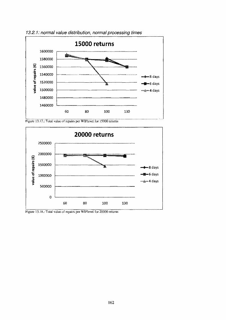
13.2.1: normal value distribution, normal processing times

15000 retu rns1600000

1580000

~ 1560000III...'j; 1540000Q.CIl...- 15200000CIl:::J'ia 1500000>

1480000

1460000

60 80 100 130

-t-8 days

_6 days

-""4 days

Figure 13.17.: Total value ofrepairs per WIPlevel for 15000 returns

20000 returns2500000

2000000I~

.....III.= 1500000IIIQ.CIl...-0 1000000CIl:::J'ia> 500000

0

60 80 100

-.....8 days

_6 days

-....4 days

130

Figure 13.18.: Total value of repairs per WIPlevel for 20000 returns

162

30000 returns2560000

2540000

2520000

2: 2500000III...'iii 2480000c.~ 2460000-o 2440000CIl

.= 2420000~

2400000

2380000

2360000

-- - .4

~ -.-..

""""-+-8 days

___6 days

.........4 days

60 80 100 130

Figure 13.19.: Total value of repairs per WIPlevel for 30000 returns

13.2.2: high value distribution, normal processing times

15000 returns2420000

2400000

2: 2380000III... 2360000'iiic.CIl 2340000...-0CIl 2320000:::JI'll 2300000>

2280000

2260000

-+-4 days

___ 6 days

.........8 days

40 60 80 100 130

Figure 13.20.: Total value of repairs per WIPlevel for 15000 returns

163

2850000

2800000

20000 returns3000000

2950000

III

"i; 2900000CoQj.......oQj:sj

2750000

""""4 days

""""6 days

~8days

40 60 80 100 130

Figure 13.21.: Total value of repairs per WIPlevel for 20000 returns

30000 returns4000000

3950000gIII...

"iQ 3900000CoQj.......0 3850000Qj:s

"iQ> 3800000

3750000

""""4 days

........ 6 days

~8days

~10days

40 60 80 100 130

Figure 13.22.: Total value of repairs per WIP1evel for 30000 returns

164

13.2.3: low value distribution, normal processing times

15000 returns1030000

1025000

2: 1020000III...'iii 1015000a.CIl....... 10100000CIl::::J

1005000'iii>

1000000

995000

60 80 100 130

Figure 13.23.: Total value of repairs per WIP1evei for 15000 returns

20000 returns

~4days

~6days

..........8 days

1240000

1230000

2: 1220000III.=III 1210000a.CIl....... 12000000CIl::::J'iii 1190000>

1180000

1170000

~4days

~6days

"""""8 days

60 80 100 130

Figure 13.24.: Total value of repairs per WIPlevel for 20000 returns

165

300000 returns1600000

1580000

2:III 1560000.=IIID.Qj 1540000...-0Qj

1520000:::JIII>

1500000

1480000

60 80 100 130

Figure 13.25.: Total value of repairs per WIPlevel for 30000 returns

13.2.4: normal value distribution, low processing times

15000 returns1700000

1680000

2: 1660000III...·iii 1640000D.Qj...- 16200000Qj:::J"iii 1600000>

1580000

1560000

60 80 100 130

Figure 13.26.: Total value of repairs per WIPlevel for 15000 returns

166

.....-4 days

""""6 days

........8 days

~lOdays

""'-4 days

""""6 days

........8 days

~10days

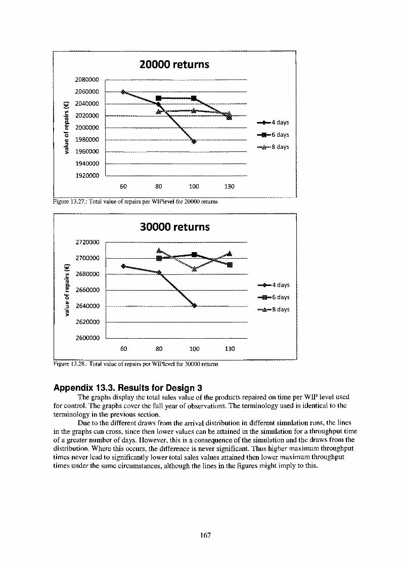
20000 returns2080000

2060000

g 2040000III... 2020000.;ac.Gl 2000000...-0Gl 1980000:::J

iO 1960000>

1940000

1920000

60 80 100 130

......4 days

-11-6 days

.......-8 days

Figure 13.27.: Total value of repairs per WIPlevel for 20000 returns

30000 returns2720000

2700000gIII 2680000...•;aC.Gl 2660000...-0Gl 2640000:::J

iO>

2620000

2600000

"""4 days

-11-6 days

.......8 days

60 80 100 130

Figure 13.28.: Total value of repairs per WIPlevel for 30000 returns

Appendix 13.3. Results for Design 3The graphs display the total sales value of the products repaired on time per WIP level used

for control. The graphs cover the full year of observations. The terminology used is identical to theterminology in the previous section.

Due to the different draws from the arrival distribution in different simulation runs, the linesin the graphs can cross, since then lower values can be attained in the simulation for a throughput timeof a greater number of days. However, this is a consequence of the simulation and the draws from thedistribution. Where this occurs, the difference is never significant. Thus higher maximum throughputtimes never lead to significantly lower total sales values attained then lower maximum throughputtimes under the same circumstances, although the lines in the figures might imply to this.

167

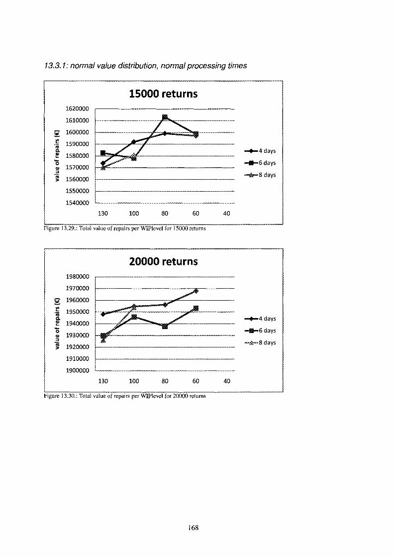
13.3. 1: normal value distribution, normal processing times

15000 returns1620000

1610000

2: 1600000III... 1590000'jija.QI 1580000...-0 1570000QI::J

iii 1560000>

1550000

1540000

130 100 80 60 40

.....4 days

_6 days

"""8 days

Figure 13.29.: Total value of repairs per WIPlevel for 15000 returns

20000 returns1980000

1970000

2: 1960000III... 1950000'jija.QI 1940000...-0 1930000QI::J

I'll 1920000>

1910000

1900000

130 100 80 60

""'4 days

_6days

......8 days

40

Figure 13.30.: Total value of repairs per WIPlevel for 20000 returns

168

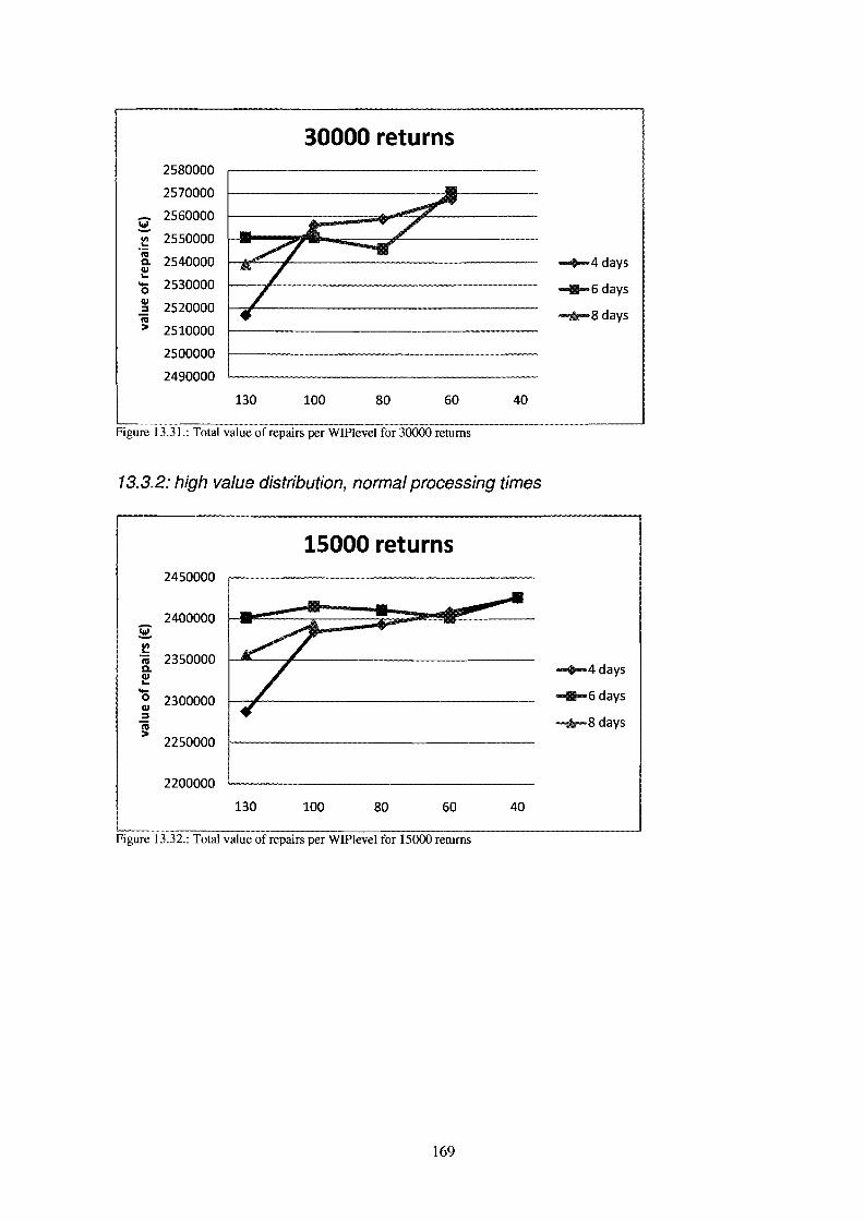
30000 returns25S0000

2570000

2:2560000

VI 2550000.:ra

2540000c.CIl...- 25300000CIl 2520000:::Jiii> 2510000

2500000

2490000

130 100 SO 60

Figure 13.31.: Total value of repairs per WIPlevel for 30000 returns

40

.......4 days

""""6 days

........Sdays

13.3.2: high value distribution, normal processing times

15000 returns2450000

24000002:VI.: 2350000rac.CIl...-0 2300000CIl:::Jiii> 2250000

2200000

130 100 SO 60 40

Figure 13.32.: Total value of repairs per WIPlevel for 15000 returns

169

.......4 days

""""6 days

........Sdays

20000 returns3000000

2950000

2:III 2900000"-'iiiD.Ql 2850000"-....0Ql

2800000::J

I'll>

2750000

2700000

130 100 80 60 40

Figure 13.33.: Total value of repairs per WIPlevel for 20000 returns

30000 returns

4050000

4000000

2: 3950000III"-'iii 3900000D.Ql"-.... 38500000Ql::J'iii 3800000>

3750000

3700000

130 100 80 60 40

Figure 13.34.: Total value of repairs per WIPlevel for 30000 returns

170

-.-4 days

""'-6 days

""""'8 days

-.-4 days

.....-6 days

.........8 days

13.303: low value distribution, normal processing times

15000 returns1040000

1020000

2: 1000000III... 9800000iija.CII 960000.......0

940000CII

-=III 920000>

900000

880000

130 100 80 60

Figure 13.35.: Total value of repairs per WIPlevel for 15000 returns

20000 returns1260000

1240000

2: 1220000III...

0iij1200000a.

CII....... 11800000CII

-= 1160000III>

1140000

1120000

130 100 80 60

Figure 13.36.: Total value of repairs per WIPlevel for 20000 returns

171

40

40

-t-4days

-B-6days

.........8 days

-t-4days

-B-6days

.........8 days

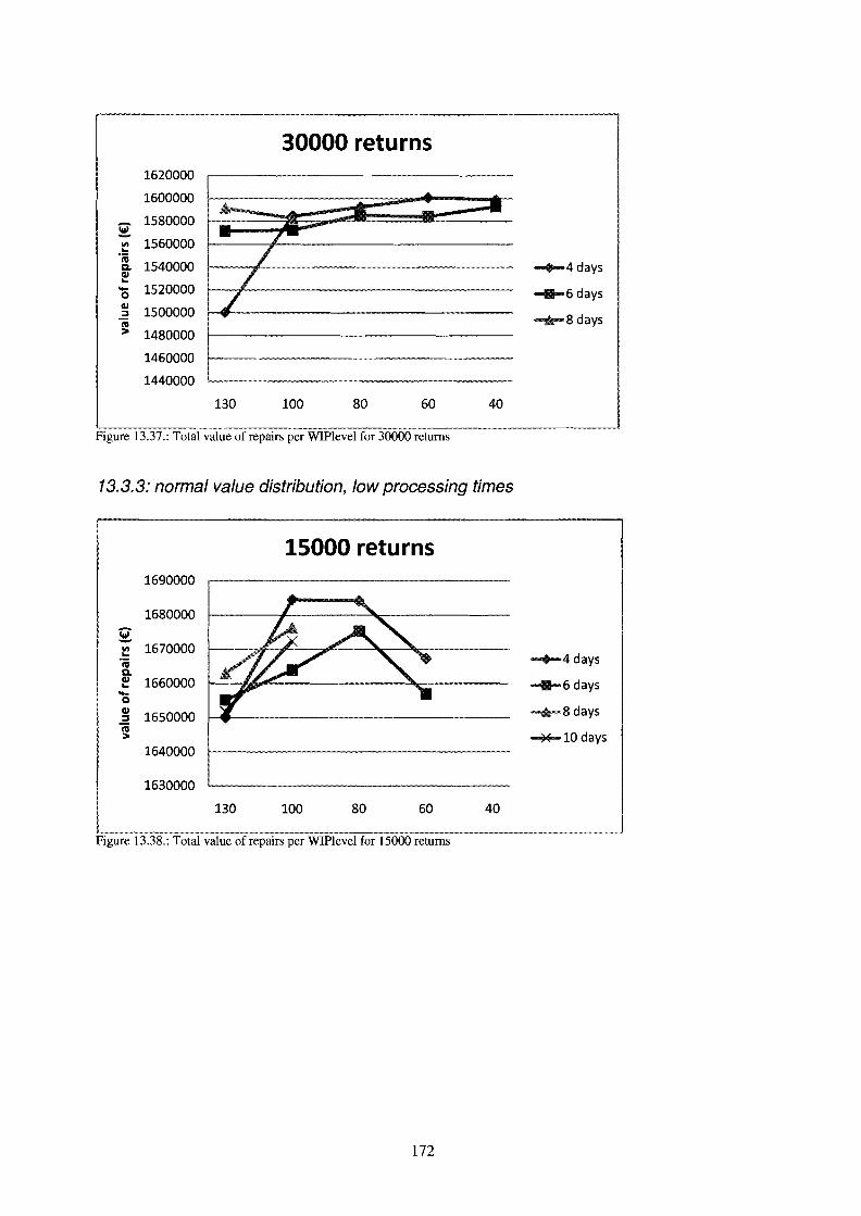
30000 returns1620000

1600000

15S0000~III 1560000...OJ;

1540000Q.111...- 15200000111 1500000:::JIII> 14S0000

1460000

1440000

130 100 SO 60 40

Figure 13.37.: Total value of repairs per WIPlevel for 30000 returns

13.3.3: normal value distribution, low processing times

15000 returns1690000

16S0000

~III 1670000.:IIIQ.111 1660000...-0111 1650000:::J'iii>

1640000

1630000

130 100 SO 60 40

Figure 13.38.: Total value of repairs per WIPlevel for 15000 returns

172

-t-4days

_6 days

........Sdays

-t-4days

_6 days

........Sdays

~10days

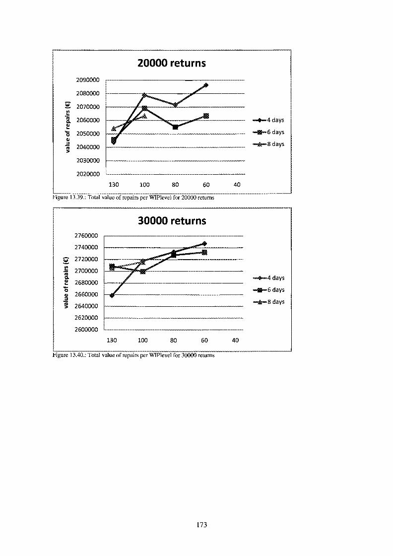
20000 returns2090000

2080000

2: 2070000III..."jij 2060000c.III...- 20500000III:::I;a 2040000>

2030000

2020000

130 100 80 60

Figure 13.39.: Total value of repairs per WIPlevel for 20000 returns

30000 returns

40

"""'4 days

""""'6 days

"""'-8 days

2760000

2740000

2: 2720000III... 2700000"jijc.III 2680000...-0 2660000III:::I

~ 2640000

2620000

2600000

130 100 80 60 40

Figure 13.40.: Total value of repairs per WIPlevel for 30000 returns

173

.......4 days

.........6 days

"""'-8 days

Appendix 13.4: Result for design 1-3

Returns per year: 15000 20000 30000

I\Jr of days maximum Total value Total value Total value

normal value distribution, normal processing times

4 97.8% 98.3% 97.3%

6 98.7% 97.6% 97.4%

8 96.7% 97.6% 96.8%

10 98.2% 97.1% 96.4%

high value distribution, normal processing times

4 96.5% 95.8% 94.9%

6 96.5% 95.4% 95.7%

8 95.2% 94.7% 95.0%

10 95.3% 96.1% 94.6%

low value distribution, normal processing times

4 99.6% 98.1% 99.1%

6 98.6% 97.0% 98.6%

8 98.3% 96.7% 98.5%

10 99.5% 97.6% 98.6%

normal value distribution, low processing times

4 99.9% 98.8% 98.9%

6 98.2% 98.0% 98.4%

8 98.3% 97.7% 97.8%

10 98.1% 97.6% 97.4%Table 13.17: Percentages of the upper bound for desIgns 1-3

174

Appendix 15: Results for varying capacity for design 3The figures show the relation between total sales value of the repaired products in euro (y­

axis) and the WIPlevel used for control in products (x-axis).

Appendix 15.1: normal value distribution, normal processing times

1man

1020304060

-+-1 man'f------------------

1400000

1200000

1000000 ~....800000

600000

400000

200000

0

100 80

Figure 15.1.: Total value of repairs per WIPlevel for 1 man capacity

1,5 man

1800000 -,------------------­

1600000 I-------==:::::;;;;;;;;..;;;;;;;;;;;;;;;;;;;;;;F;;;;;;;;;;;~"'~­

1400000 +--~---,a__--:::.........:::..-......_--------

1200000 'f---"----------------­

1000000 'f------------------800000 -1- ~1/5man

600000 'f------------------

400000 'f------------------

200000 -1------------------o 'f---,-----;r----,----,-----,----,

100 80 60 40 30 20

Figure 15.2.: Total value of repairs per WIPlevel for 1,5 men capacity

175

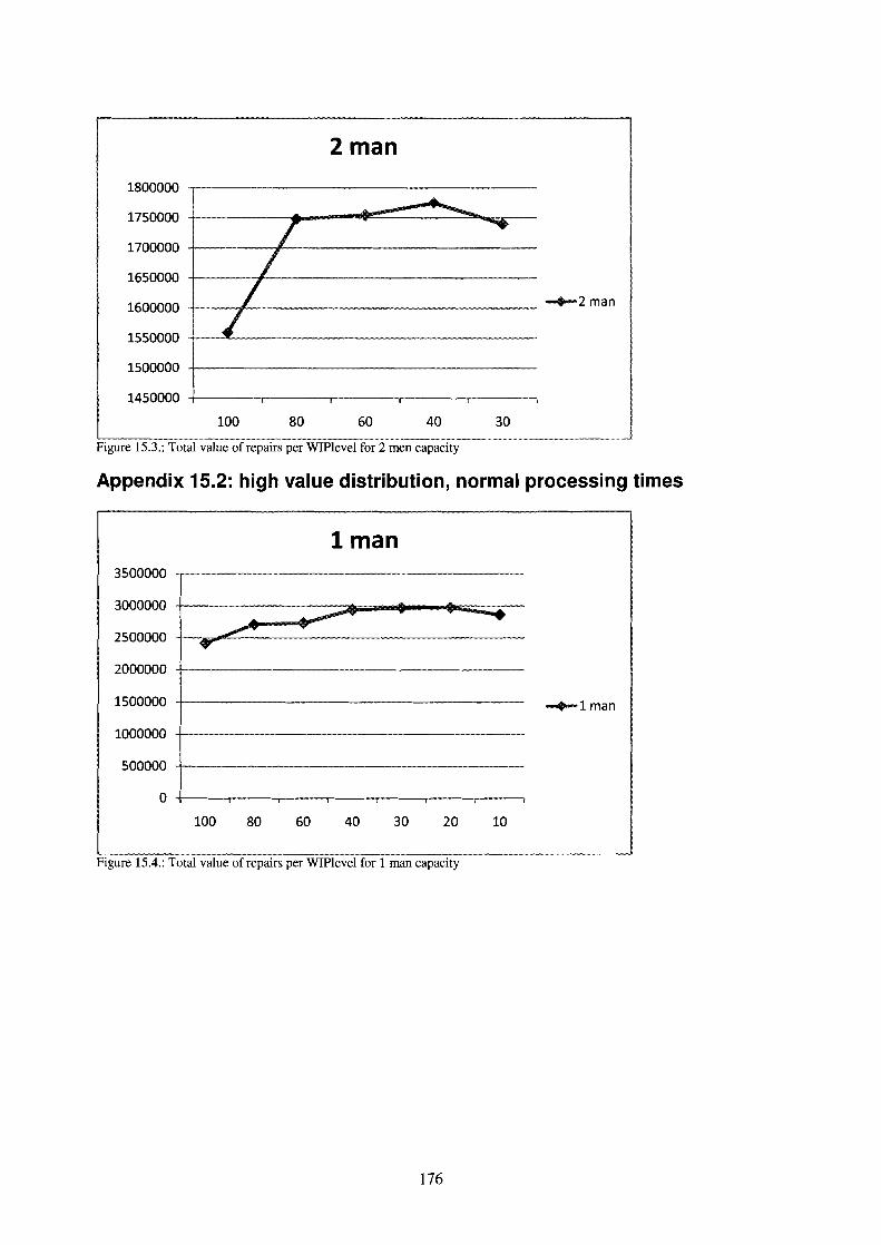
2man

1800000

1750000

1700000

1650000

1600000

1550000

1500000

1450000

.-.................

/ ......

//~

-+-2 man

100 80 60 40 30

Figure 15.3.: Total value ofrepairs per WIPlevel for 2 men capacity

Appendix 15.2: high value distribution, normal processing times

lman3500000

3000000

2500000

2000000

1500000

1000000

500000

o

~.". ......

~.,

-+-1 man

100 80 60 40 30 20 10

Figure 15.4.: Total value of repairs per WIPlevel for 1 man capacity

176

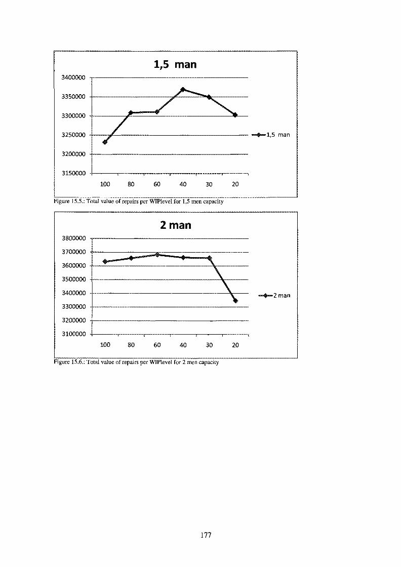
1,5 man

+---:#"----------------- ......1,5 man

3200000

3150000 -j---.----.----,---,---,------,

3350000

3250000

3300000

3400000

100 80 60 40 30 20

Figure 15.5.: Total value ofrepairs per WIPlevel for 1,5 men capacity

2man3800000

3700000

3600000

3500000

3400000

3300000

... '\.

\\'.

3200000

3100000

100 80 60 40 30 20

Figure 15.6.: Total value ofrepairs per WIPlevel for 2 men capacity

177

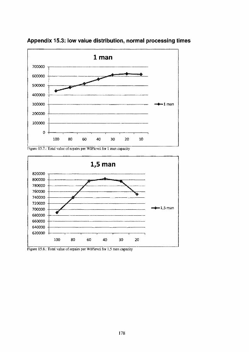
Appendix 15.3: low value distribution, normal processing times

1man700000 ..,-------------------

....600000 +-----~-----:::;;ooooI .....~~~~~-500000 +--~----rc"""""~::!:------------

400000 -t-------------------

300000 +-------------------

200000 +-------------------

100000 +-------------------

0+------.---.---..----..---.------.---,

100 80 60 40 30 20 10

Figure 15.7.: Total value of repairs per WIPlevel for 1 man capacity

1,5 man820000800000780000760000740000720000700000680000660000640000620000

.A..

r '-/ "-/ ...

/'/"

~

100 80 60 40 30 20

Figure 15.8.: Total value of repairs per WIPlevel for 1,5 men capacity

178

2man940000

920000

900000 +----~----------~--­

880000

860000

840000

820000 +---,---,---....,----,-----.---,

100 80 60 40 30 20

Figure 15.9.: Total value ofrepairs per WIPlevel for 2 men capacity

179

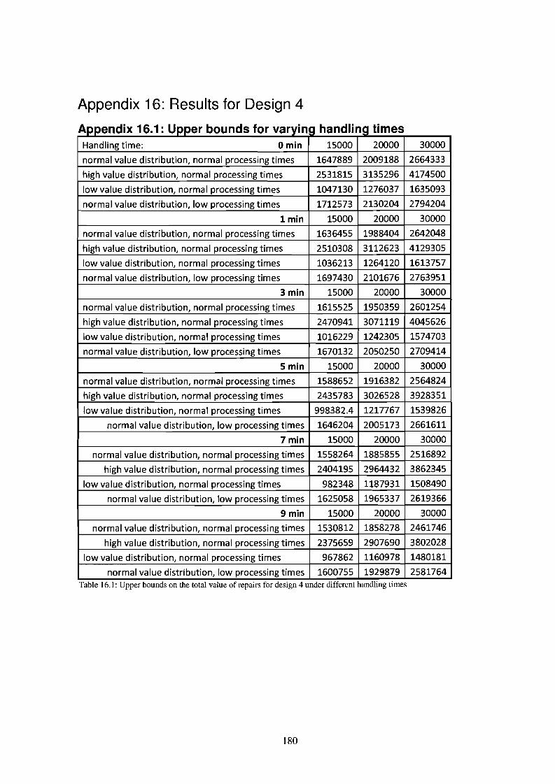
Appendix 16: Results for Design 4

A d" 16 1 U b d f h dr~ppen IX " Ipper oun s or varVIna an Ina times" "

Handling time: Omin 15000 20000 30000

normal value distribution, normal processing times 1647889 2009188 2664333

high value distribution, normal processing times 2531815 3135296 4174500

low value distribution, normal processing times 1047130 1276037 1635093

normal value distribution, low processing times 1712573 2130204 2794204

lmin 15000 20000 30000

normal value distribution, normal processing times 1636455 1988404 2642048

high value distribution, normal processing times 2510308 3112623 4129305

low value distribution, normal processing times 1036213 1264120 1613757

normal value distribution, low processing times 1697430 2101676 2763951

3min 15000 20000 30000

normal value distribution, normal processing times 1615525 1950359 2601254

high value distribution, normal processing times 2470941 3071119 4045626

low value distribution, normal processing times 1016229 1242305 1574703

normal value distribution, low processing times 1670132 2050250 2709414

Smin 15000 20000 30000

normal value distribution, normal processing times 1588652 1916382 2564824

high value distribution, normal processing times 2435783 3026528 3928351

low value distribution, normal processing times 998382.4 1217767 1539826

normal value distribution, low processing times 1646204 2005173 2661611

7min 15000 20000 30000

normal value distribution, normal processing times 1558264 1885855 2516892

high value distribution, normal processing times 2404195 2964432 3862345

low value distribution, normal processing times 982348 1187931 1508490

normal value distribution, low processing times 1625058 1965337 2619366

9min 15000 20000 30000

normal value distribution, normal processing times 1530812 1858278 2461746

high value distribution, normal processing times 2375659 2907690 3802028

low value distribution, normal processing times 967862 1160978 1480181

normal value distribution, low processing times 1600755 1929879 2581764Table 16.1: Upper bounds on the total value of repairs for desIgn 4 under dIfferent handlmg tImes

180