Elastic Tail Propulsion at Low Reynolds Number

by

Tony S. Yu

B.S. Mechanical EngineeringColumbia University, 2004

Submitted to the Department of Mechanical Engineeringin partial fulfillment of the requirements for the degree of

Master of Science in Mechanical Engineering

at the

MASSACHUSETTS INSTITUTE OF TECHNOLOGY

January 2007

c© Massachusetts Institute of Technology 2007. All rights reserved.

Author . . . . . . . . . . . . . . . . . . . . . . . . . . . . . . . . . . . . . . . . . . . . . . . . . . . . . . . . . . . . . .Department of Mechanical Engineering

January 19, 2007

Certified by. . . . . . . . . . . . . . . . . . . . . . . . . . . . . . . . . . . . . . . . . . . . . . . . . . . . . . . . . .Anette E. Hosoi

Associate Professor, Mechanical EngineeringThesis Supervisor

Accepted by . . . . . . . . . . . . . . . . . . . . . . . . . . . . . . . . . . . . . . . . . . . . . . . . . . . . . . . . .Lallit Anand

Chairman, Department Committee on Graduate Students

2

Elastic Tail Propulsion at Low Reynolds Number

by

Tony S. Yu

Submitted to the Department of Mechanical Engineeringon January 19, 2007, in partial fulfillment of the

requirements for the degree ofMaster of Science in Mechanical Engineering

Abstract

A simple way to generate propulsion at low Reynolds number is to periodically oscil-late a passive flexible filament. Here we present a macroscopic experimental investi-gation of such a propulsive mechanism. A robotic swimmer is constructed and bothtail shape and propulsive force are measured. Filament characteristics and the actu-ation are varied and resulting data are quantitatively compared with existing linearand nonlinear theories.

Thesis Supervisor: Anette E. HosoiTitle: Associate Professor, Mechanical Engineering

4

Acknowledgments

I would like to thank my advisor Anette “Peko” Hosoi; she has been an encouraging

and supportive mentor since the day I first stumbled into her office. I hope in the

future I will be able to balance teaching, research, and life as well as she does.

I could not have gotten through the tough times without the support and friend-

ship of Sungyon Lee and Danielle Chou. Also, a special thanks to Eric Lauga for his

advice on research and music.

Finally, love and thanks to my family, who have been supportive in all my ventures

and to my lab mates, who have been like a second family to me.

6

Contents

1 Introduction 13

1.1 Low Reynolds Number Swimming . . . . . . . . . . . . . . . . . . . . 13

1.2 Motivation . . . . . . . . . . . . . . . . . . . . . . . . . . . . . . . . . 18

1.3 Thesis Summary . . . . . . . . . . . . . . . . . . . . . . . . . . . . . 19

2 Theory of Elastic Tail Swimming 21

2.1 Stokes Flow and Reversibility . . . . . . . . . . . . . . . . . . . . . . 21

2.2 Slender Body Hydrodynamics . . . . . . . . . . . . . . . . . . . . . . 23

2.3 Elastic Forces . . . . . . . . . . . . . . . . . . . . . . . . . . . . . . . 24

2.4 Nonlinear Equations . . . . . . . . . . . . . . . . . . . . . . . . . . . 25

2.5 Linear Equation . . . . . . . . . . . . . . . . . . . . . . . . . . . . . . 26

2.6 Boundary Conditions . . . . . . . . . . . . . . . . . . . . . . . . . . . 27

2.7 Propulsive Force . . . . . . . . . . . . . . . . . . . . . . . . . . . . . 30

3 Methods and Implementation 33

3.1 Robotic Swimmer—“RoboChlam” . . . . . . . . . . . . . . . . . . . . 33

3.2 Fixed Swimmer Experiment . . . . . . . . . . . . . . . . . . . . . . . 34

3.3 Propulsive Force Measurement . . . . . . . . . . . . . . . . . . . . . . 35

3.3.1 Beam Theory . . . . . . . . . . . . . . . . . . . . . . . . . . . 36

3.3.2 Strain Gages . . . . . . . . . . . . . . . . . . . . . . . . . . . 37

3.3.3 Wheatstone Bridge Circuit . . . . . . . . . . . . . . . . . . . . 37

3.3.4 Voltage Amplifiers . . . . . . . . . . . . . . . . . . . . . . . . 38

3.3.5 Procedure for Force Measurement . . . . . . . . . . . . . . . . 39

7

3.4 Tail Shape (Waveform) Comparison . . . . . . . . . . . . . . . . . . . 42

3.4.1 Video Acquisition . . . . . . . . . . . . . . . . . . . . . . . . . 42

3.4.2 Image Processing . . . . . . . . . . . . . . . . . . . . . . . . . 43

3.4.3 Comparing Experimental and Theoretical Tail Shapes . . . . . 43

3.5 Numerical Solution of Nonlinear Equations . . . . . . . . . . . . . . . 45

3.5.1 Newton’s Method of Root-Finding . . . . . . . . . . . . . . . 46

3.5.2 Finite Difference Equation . . . . . . . . . . . . . . . . . . . . 47

3.5.3 Newton’s Method in Multiple Dimensions . . . . . . . . . . . 49

3.6 Wall Effects . . . . . . . . . . . . . . . . . . . . . . . . . . . . . . . . 50

4 Results and Discussion 53

4.1 Propulsive Force . . . . . . . . . . . . . . . . . . . . . . . . . . . . . 53

4.2 Tail Shapes . . . . . . . . . . . . . . . . . . . . . . . . . . . . . . . . 55

5 Conclusions 57

A Additional Figures and Tables 59

B Solution of Governing Equations 65

B.1 Elastic Force of Slender Rod . . . . . . . . . . . . . . . . . . . . . . . 65

B.2 Nonlinear Equations of Motion . . . . . . . . . . . . . . . . . . . . . 67

B.3 Linear Equations of Motion . . . . . . . . . . . . . . . . . . . . . . . 68

B.4 Linear Propulsive Force . . . . . . . . . . . . . . . . . . . . . . . . . . 70

8

List of Figures

1-1 Transmission Electron Microscopy (TEM) image of Escherichia coli. . 14

1-2 Sketches of theoretical swimmers from Purcell’s Life at Low Reynolds

Numbers [26]. . . . . . . . . . . . . . . . . . . . . . . . . . . . . . . . 15

1-3 Diagram from [33] of G.I. Taylor’s device to test his theory of waving

cylindrical tails. . . . . . . . . . . . . . . . . . . . . . . . . . . . . . . 16

1-4 Experimental work by Chan and Hosoi on the motion of the three-link

swimmer [6]. . . . . . . . . . . . . . . . . . . . . . . . . . . . . . . . . 16

1-5 Simulation of pumping motion of angularly-oscillated filaments from

Kim et al. [16]. . . . . . . . . . . . . . . . . . . . . . . . . . . . . . . 18

2-1 Schematic of a hypothetical scallop at low Reynolds number. . . . . . 22

2-2 Slender cylinders in a low Reynolds number flow. . . . . . . . . . . . 23

2-3 Elastic tail with tail base at the origin. . . . . . . . . . . . . . . . . . 24

2-4 Elastic tail with an antisymmetric, imaginary tail attached at base. . 29

3-1 Robotic elastic-tail swimmer. . . . . . . . . . . . . . . . . . . . . . . 33

3-2 Scotch yoke and lever mechanism. . . . . . . . . . . . . . . . . . . . . 35

3-3 Schematic of experimental setup. . . . . . . . . . . . . . . . . . . . . 35

3-4 Diagram of cantilever beam. . . . . . . . . . . . . . . . . . . . . . . . 36

3-5 Diagram of circuit for strain gage measurement. . . . . . . . . . . . . 38

3-6 Photograph of experimental setup. . . . . . . . . . . . . . . . . . . . 42

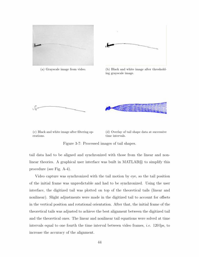
3-7 Processed images of tail shapes. . . . . . . . . . . . . . . . . . . . . . 44

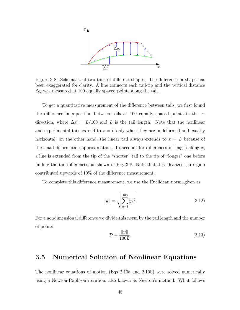
3-8 Schematic of two tails of different shapes. . . . . . . . . . . . . . . . . 45

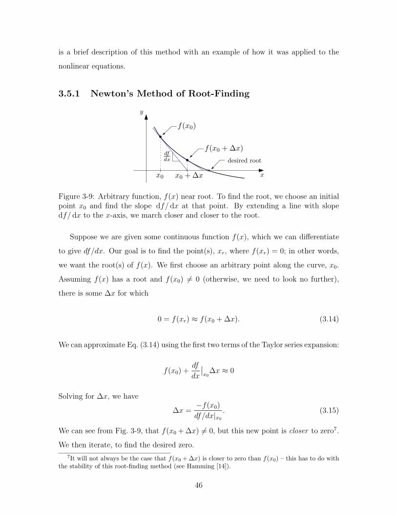
3-9 Arbitrary function, f(x) near root. . . . . . . . . . . . . . . . . . . . 46

9

3-10 Discrete version of elastic tail. . . . . . . . . . . . . . . . . . . . . . . 47

3-11 Schematic of slender rod near a wall. . . . . . . . . . . . . . . . . . . 52

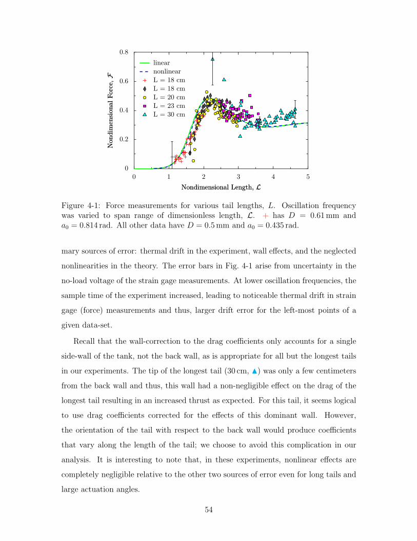
4-1 Force measurements for various tail lengths. . . . . . . . . . . . . . . 54

4-2 Comparison of three tail shapes. . . . . . . . . . . . . . . . . . . . . . 55

4-3 Normalized, time-averaged difference between tail shapes. . . . . . . . 56

5-1 Free-swimming RoboChlam . . . . . . . . . . . . . . . . . . . . . . . 58

A-1 Sample strain gage voltage (force) curve. . . . . . . . . . . . . . . . . 59

A-2 Sample force calibration measurement. . . . . . . . . . . . . . . . . . 60

A-3 Screenshot of user interface for video processing. . . . . . . . . . . . . 62

A-4 Screenshot of user interface for comparing experimental and theoretical

tail-shapes. . . . . . . . . . . . . . . . . . . . . . . . . . . . . . . . . 63

10

List of Tables

1.1 Previous work on elastic-tail swimmers. . . . . . . . . . . . . . . . . . 17

2.1 Physical interpretations of the tail shape and derivatives of the tail

shape. . . . . . . . . . . . . . . . . . . . . . . . . . . . . . . . . . . . 28

2.2 Boundary conditions on linear equations. . . . . . . . . . . . . . . . . 28

2.3 Boundary conditions on coupled nonlinear equations. . . . . . . . . . 30

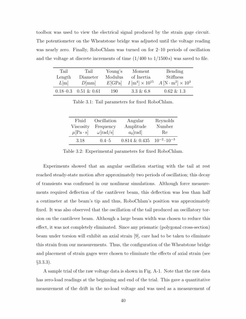
3.1 Tail parameters for fixed RoboChlam. . . . . . . . . . . . . . . . . . . 40

3.2 Experimental parameters for fixed RoboChlam. . . . . . . . . . . . . 40

3.3 Cantilever beam parameters. . . . . . . . . . . . . . . . . . . . . . . . 41

3.4 Parameters for the strain gage circuit. . . . . . . . . . . . . . . . . . . 41

3.5 Derivatives of finite differences. . . . . . . . . . . . . . . . . . . . . . 50

A.1 Finite differences and their derivatives. . . . . . . . . . . . . . . . . . 61

11

12

Chapter 1

Introduction

Swimming at micro-scales has long been the realm of bacteria and other micro-

organisms [3, 20], but recent advances in fabrication and manipulation at small scales

have allowed researchers to catch up with nature [11]. At these small scales, the

physics of swimming is fundamentally different than at human scales because the vis-

cous forces of the fluid dominate inertial forces. Imagine falling into a swimming pool

filled with honey; if we only considered inertial forces, it would seem that swimming

in this pool should not be so different than swimming in a water-filled pool, because

inertia is simply proportional to density and the density of honey is nearly the same

as that of water. In reality, we expect it to be much harder to swim in honey because

honey is “thicker”—or to be precise: more viscous—than water. Now if we return to

a normal water-filled pool and shrink to the size of a bacterium, a funny thing occurs:

this aqueous environment would appear to the bacteria much like that honey-filled

pool. This similarity is determined by the Reynolds number of the flow. In this the-

sis, we focus on cases where the Reynolds number is small and hence viscous forces

dominate.

1.1 Low Reynolds Number Swimming

The relative importance of inertial and viscous forces is reflected in the Reynolds

number of the flow: Re = V L/ν, where ν is the kinematic viscosity of the fluid, V

13

Figure 1-1: Transmission Electron Microscopy (TEM) image of Escherichia coli withmultiple helical flagella from http://www.astrographics.com/ – Dennis Kunkel.

is a characteristic velocity, and L is a characteristic length. If the Reynolds number

is low (i.e. Re " 1), viscous forces dominate inertial forces. In contrast to the

honey-filled pool at the beginning of this chapter, low Reynolds number flows usually

involve small scales and low velocities since many common fluids have relatively small

kinematic viscosities (νwater ≈ 10−6, νair ≈ 10−5)1. For example, consider a vertically-

challenged human of one meter in height; he would need to move at a rate of less than

1 µm/s in water to be considered a low Reynolds number swimmer! Thus, when we

speak of “low Reynolds number swimming”, we are generally referring to incredibly

small swimmers, i.e. micro-organisms. For E. coli, with L ≈ 3 µm and V ≈ 30 µm/s

[4], the Reynolds number is 10−4; this can certainly be considered small and inertial

forces are quite negligible. Low Reynolds number flow is also referred to as Stokes

flow, creeping flow, or viscous flow and can have peculiar effects that are very different

from those observed in our inertia-dominated world.

When viscous forces dominate, it is not simply “harder” to swim, as one might

expect from the honey-filled pool analogy. To produce net translation in these con-

ditions, the swimming motion must be both cyclic and non-reciprocal, as described

by E.M. Purcell in his famous lecture, Life at Low Reynolds Numbers [26]. Much like

the cyclic butterfly stroke of a human swimmer, any self-propelling motion should

1This is not always the case, of course—as exemplified by the unfortunate insects that get trappedin tree resin and become fossilized in amber.

14

be periodic if you want to generate continuous, net motion2. This requirement is

especially true in Stokesian regimes because viscous forces quickly kill the velocity

generated by a single stroke3. The second condition is required because a reciprocal

motion leaves a swimmer oscillating in place, as shown by the “Scallop Theorem”

(see [26] and §2.1).

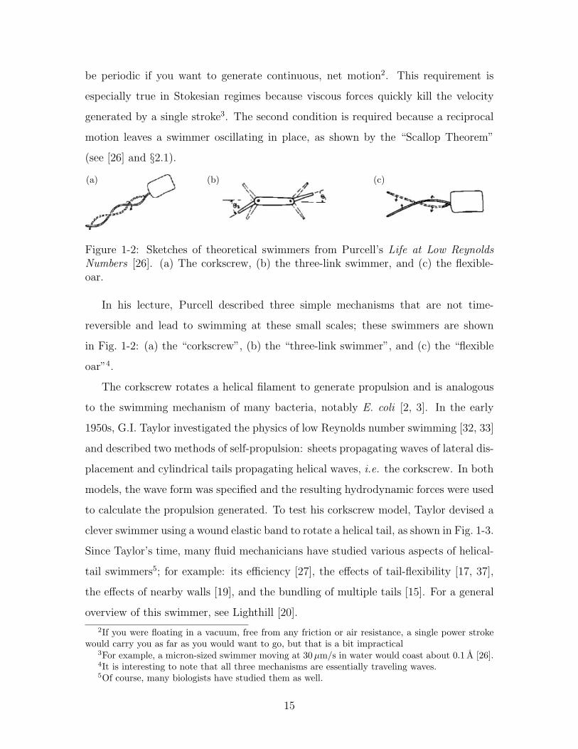
(a) (b) (c)

Figure 1-2: Sketches of theoretical swimmers from Purcell’s Life at Low ReynoldsNumbers [26]. (a) The corkscrew, (b) the three-link swimmer, and (c) the flexible-oar.

In his lecture, Purcell described three simple mechanisms that are not time-

reversible and lead to swimming at these small scales; these swimmers are shown

in Fig. 1-2: (a) the “corkscrew”, (b) the “three-link swimmer”, and (c) the “flexible

oar”4.

The corkscrew rotates a helical filament to generate propulsion and is analogous

to the swimming mechanism of many bacteria, notably E. coli [2, 3]. In the early

1950s, G.I. Taylor investigated the physics of low Reynolds number swimming [32, 33]

and described two methods of self-propulsion: sheets propagating waves of lateral dis-

placement and cylindrical tails propagating helical waves, i.e. the corkscrew. In both

models, the wave form was specified and the resulting hydrodynamic forces were used

to calculate the propulsion generated. To test his corkscrew model, Taylor devised a

clever swimmer using a wound elastic band to rotate a helical tail, as shown in Fig. 1-3.

Since Taylor’s time, many fluid mechanicians have studied various aspects of helical-

tail swimmers5; for example: its efficiency [27], the effects of tail-flexibility [17, 37],

the effects of nearby walls [19], and the bundling of multiple tails [15]. For a general

overview of this swimmer, see Lighthill [20].

2If you were floating in a vacuum, free from any friction or air resistance, a single power strokewould carry you as far as you would want to go, but that is a bit impractical

3For example, a micron-sized swimmer moving at 30µm/s in water would coast about 0.1 A [26].4It is interesting to note that all three mechanisms are essentially traveling waves.5Of course, many biologists have studied them as well.

15

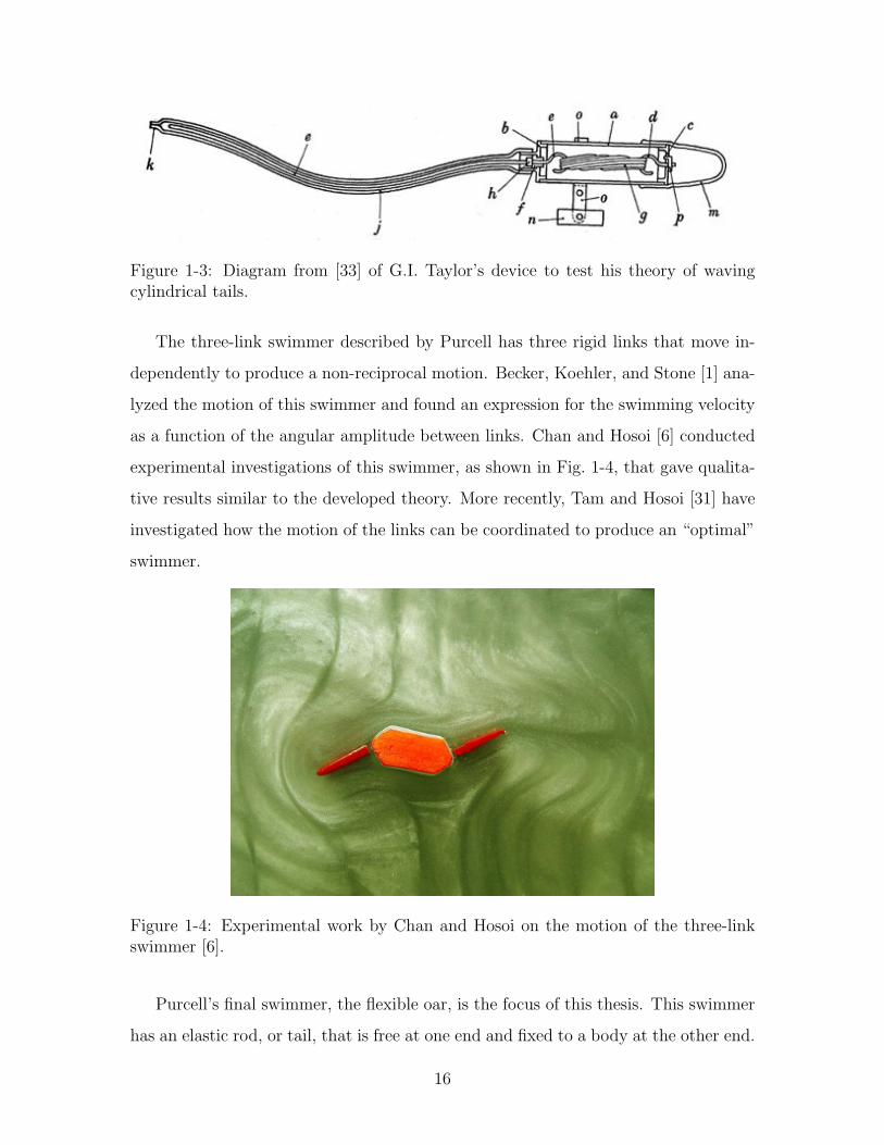
Figure 1-3: Diagram from [33] of G.I. Taylor’s device to test his theory of wavingcylindrical tails.

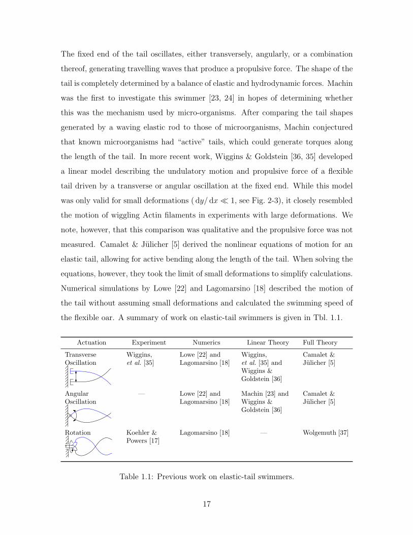
The three-link swimmer described by Purcell has three rigid links that move in-

dependently to produce a non-reciprocal motion. Becker, Koehler, and Stone [1] ana-

lyzed the motion of this swimmer and found an expression for the swimming velocity

as a function of the angular amplitude between links. Chan and Hosoi [6] conducted

experimental investigations of this swimmer, as shown in Fig. 1-4, that gave qualita-

tive results similar to the developed theory. More recently, Tam and Hosoi [31] have

investigated how the motion of the links can be coordinated to produce an “optimal”

swimmer.

Figure 1-4: Experimental work by Chan and Hosoi on the motion of the three-linkswimmer [6].

Purcell’s final swimmer, the flexible oar, is the focus of this thesis. This swimmer

has an elastic rod, or tail, that is free at one end and fixed to a body at the other end.

16

The fixed end of the tail oscillates, either transversely, angularly, or a combination

thereof, generating travelling waves that produce a propulsive force. The shape of the

tail is completely determined by a balance of elastic and hydrodynamic forces. Machin

was the first to investigate this swimmer [23, 24] in hopes of determining whether

this was the mechanism used by micro-organisms. After comparing the tail shapes

generated by a waving elastic rod to those of microorganisms, Machin conjectured

that known microorganisms had “active” tails, which could generate torques along

the length of the tail. In more recent work, Wiggins & Goldstein [36, 35] developed

a linear model describing the undulatory motion and propulsive force of a flexible

tail driven by a transverse or angular oscillation at the fixed end. While this model

was only valid for small deformations ( dy/ dx " 1, see Fig. 2-3), it closely resembled

the motion of wiggling Actin filaments in experiments with large deformations. We

note, however, that this comparison was qualitative and the propulsive force was not

measured. Camalet & Julicher [5] derived the nonlinear equations of motion for an

elastic tail, allowing for active bending along the length of the tail. When solving the

equations, however, they took the limit of small deformations to simplify calculations.

Numerical simulations by Lowe [22] and Lagomarsino [18] described the motion of

the tail without assuming small deformations and calculated the swimming speed of

the flexible oar. A summary of work on elastic-tail swimmers is given in Tbl. 1.1.

Actuation Experiment Numerics Linear Theory Full Theory

TransverseOscillation

Wiggins,et al. [35]

Lowe [22] andLagomarsino [18]

Wiggins,et al. [35] andWiggins &Goldstein [36]

Camalet &Julicher [5]

AngularOscillation

— Lowe [22] andLagomarsino [18]

Machin [23] andWiggins &Goldstein [36]

Camalet &Julicher [5]

Rotation Koehler &Powers [17]

Lagomarsino [18] — Wolgemuth [37]

Table 1.1: Previous work on elastic-tail swimmers.

17

1.2 Motivation

As discussed in the last section, swimming at low Reynolds number usually refers to

swimming at small scales. But why would one want to build such small swimmers?

These micro-swimmers could provide propulsion for medical devices used for mini-

mally invasive surgery or targeted drug delivery. Also, micro-swimmers could easily

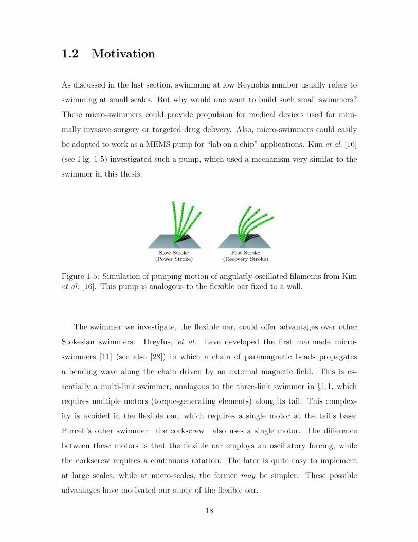
be adapted to work as a MEMS pump for “lab on a chip” applications. Kim et al. [16]

(see Fig. 1-5) investigated such a pump, which used a mechanism very similar to the

swimmer in this thesis.

Slow Stroke(Power Stroke)

Fast Stroke(Recovery Stroke)

Figure 1-5: Simulation of pumping motion of angularly-oscillated filaments from Kimet al. [16]. This pump is analogous to the flexible oar fixed to a wall.

The swimmer we investigate, the flexible oar, could offer advantages over other

Stokesian swimmers. Dreyfus, et al. have developed the first manmade micro-

swimmers [11] (see also [28]) in which a chain of paramagnetic beads propagates

a bending wave along the chain driven by an external magnetic field. This is es-

sentially a multi-link swimmer, analogous to the three-link swimmer in §1.1, which

requires multiple motors (torque-generating elements) along its tail. This complex-

ity is avoided in the flexible oar, which requires a single motor at the tail’s base;

Purcell’s other swimmer—the corkscrew—also uses a single motor. The difference

between these motors is that the flexible oar employs an oscillatory forcing, while

the corkscrew requires a continuous rotation. The later is quite easy to implement

at large scales, while at micro-scales, the former may be simpler. These possible

advantages have motivated our study of the flexible oar.

18

1.3 Thesis Summary

In this thesis, we investigate the angularly-actuated flexible oar design and test the

validity of the linear model derived in Wiggins & Goldstein [36] comparing it to

the waveforms and propulsive forces generated by a robotic, flexible-tail swimmer,

dubbed “RoboChlam”. For further comparison, we solve numerically the nonlinear

equations presented in Camalet & Julicher [5]. In the next chapter, we develop the

nonlinear and linear equations of motion, from which we also derive an expression for

the propulsive force. In Chapter 3, we describe the experiment used to test the theory

and the Newton-Raphson method, which was used to solve the nonlinear equations.

In Chapter 4, we present and discuss the results of our experiment. Finally, our

conclusions and future work are presented in Chapter 5.

19

20

Chapter 2

Theory of Elastic Tail Swimming

Here we will present the theory behind the motion of an elastic tail at low Reynolds

number. First, we review some key concepts of low Reynolds number flow, also known

as Stokes flow, and then focus on the case of slender-bodies in this regime. Next we

will solve for the elastic forces in the tail. The hydrodynamic and elastic forces are

then balanced along the tail to find the equations of motion for the tail. From these

equations, we derive a linear equation of motion and an expression for the propulsive

force generated by a waving tail.

2.1 Stokes Flow and Reversibility

In general, the motion of a Newtonian fluid is governed by the Navier-Stokes equation:

ρ∂u

∂t+ ρu ·∇u = µ∇2u−∇p. (2.1)

When the Reynolds number is low, the inertial terms in the above equation are

negligible such that

−∇p + µ∇2u = 0. (2.2)

The above equation is known as the Stokes equation and states that, in the absence of

external forces, pressure forces must balance viscous forces at all times. In addition,

conservation of mass for an incompressible fluid requires a divergence free flow, such

21

that

∇ · u = 0. (2.3)

By neglecting inertia, there exists a linear relationship between pressure forces and

velocity, as given by the Stokes equation; this linearity means that the fluid flow is

kinematically reversible, a property also known as time-reversibility (see [21, 7, 8]).

The importance of this reversibility is discussed below.

NetForce

(a)

NetForce

(b)

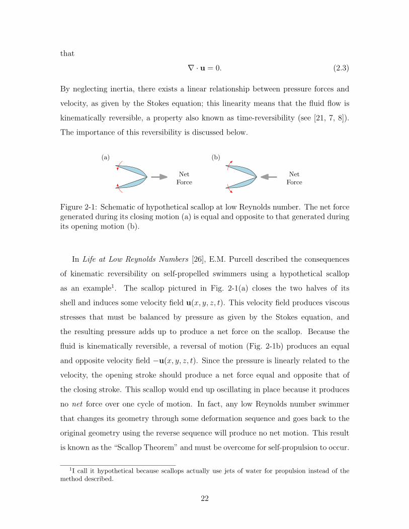
Figure 2-1: Schematic of hypothetical scallop at low Reynolds number. The net forcegenerated during its closing motion (a) is equal and opposite to that generated duringits opening motion (b).

In Life at Low Reynolds Numbers [26], E.M. Purcell described the consequences

of kinematic reversibility on self-propelled swimmers using a hypothetical scallop

as an example1. The scallop pictured in Fig. 2-1(a) closes the two halves of its

shell and induces some velocity field u(x, y, z, t). This velocity field produces viscous

stresses that must be balanced by pressure as given by the Stokes equation, and

the resulting pressure adds up to produce a net force on the scallop. Because the

fluid is kinematically reversible, a reversal of motion (Fig. 2-1b) produces an equal

and opposite velocity field −u(x, y, z, t). Since the pressure is linearly related to the

velocity, the opening stroke should produce a net force equal and opposite that of

the closing stroke. This scallop would end up oscillating in place because it produces

no net force over one cycle of motion. In fact, any low Reynolds number swimmer

that changes its geometry through some deformation sequence and goes back to the

original geometry using the reverse sequence will produce no net motion. This result

is known as the “Scallop Theorem” and must be overcome for self-propulsion to occur.

1I call it hypothetical because scallops actually use jets of water for propulsion instead of themethod described.

22

2.2 Slender Body Hydrodynamics

u⊥ u‖(b) (c)

f⊥ = ξ⊥u⊥

u(a)

f

f‖ = ξ‖u‖

n

t

Figure 2-2: Slender cylinders in a low Reynolds number flow. The drag force per unitlength, f , is linearly related to the velocity by drag coefficients ξ⊥ and ξ‖.

If the length of a body, L, is much greater than its diameter, D, (L/D & 1),

Stokes equations can be further simplified using resistive force theory [4, 13, 20].

Applying this theory to a section of the tail, the drag force in Fig. 2-2(a) is broken

down into components transverse and longitudinal to the tail axis (Fig. 2-2b and c,

respectively). Thus, the drag forces on the tail are linearly related to the velocity by

the transverse and axial drag coefficients, ξ⊥ and ξ‖. Since u⊥ = u · n and u‖ = u · t,

we see that

f⊥ = ξ⊥u · n, (2.4a)

f‖ = ξ‖u · t. (2.4b)

For a slender, cylindrical rod, these drag coefficients can be expressed as

ξ⊥ =4πµ

ln Lr + 0.193

(2.5a)

ξ‖ =2πµ

ln Lr − 0.807

(2.5b)

where µ is the viscosity of the fluid, and L and r are the length and radius of the rod.

Eqs (2.5a) and (2.5b) are functions of the aspect ratio of the rod, defined as L/r,

which by definition is quite large for a slender body. It is interesting to note that the

drag coefficients, and consequently the drag force, are weak (logarithmic) functions

of the tail radius.

To determine the drag force on the tail, we must now define a velocity. A point

23

r(s)

t(s)

n(s)

y

x

ds

ψ(s)

D

BodyTail

Figure 2-3: Elastic tail with tail base at the origin. The tail is parametrized byarclength s and has a tail shape given by the position vector r(s). Inset: tail elementwith length ds, local angle ψ, unit normal n, unit tangent t. Additionally there isa local tension τ(s) acting on the cross section and defined positive outwards (notshown).

on the tail is defined by its position vector r, as shown in Fig. 2-3, and has a velocity

rt, where the subscript t denotes a time derivative. In a quiescent fluid, the relative

velocity of the fluid would be −rt; thus, the total velocity is simply u − rt, where u

is the velocity of the fluid in the fixed frame. Now the drag force per unit length of

the rod can be expressed as

fd = −[ξ⊥nn + ξ‖tt] · (rt − u), (2.6)

where n and t are the unit normal and tangent to the filament, respectively. We

consider a planar actuation of the rod, so that n is defined without ambiguities to

remain in this plane. Note that Eq. (2.6) is simply a vector expression for Eqs (2.4a)

and (2.4b) with an additional transformation from the normal and tangent coordinates

into a fixed coordinate system.

2.3 Elastic Forces

The elastic tail, with an arc length coordinate s, can be described by the position

vector r(s), local angle ψ(s), unit normal n(s), and unit tangent t(s), as shown in

Fig. 2-3. The unit normal is described as “inward pointing” such that it points

24

towards the center of curvature, and we consider a 2-D case where n remains in the

plane. The elastic forces on the rod are derived from an energy functional which

includes its bending energy and its inextensibility constraint

E =

∫ L

0

[A

2κ2 +

Λ

2rs

2

]ds, (2.7)

where the subscript s denotes a derivative, A is the bending stiffness, κ ≡ ψs is the

curvature of the tail, and Λ is the Lagrange multiplier enforcing inextensibility. Using

calculus of variation we obtain the elastic force per unit length, fε = −δE/δr as given

by [5, 37]

fε = −(Aψsss − ψsτ)n + (Aψssψs + τs)t, (2.8)

where τ = −Λ + Aκ2 can be interpreted as the local tension in the tail. The details

of this derivation are given in §B.1.

2.4 Nonlinear Equations

Camalet & Julicher [5] derived the equations of motion for an elastic tail with torque

generating elements along the tail. Here we have a passive tail with torque generated

only at the base. Thus, the equations of motion for our swimmer are a simplified

version of those derived in [5].

We have already found expressions for the only relevant forces in the system: the

elastic forces in the tail and the drag forces from the fluid. We now enforce local

mechanical equilibrium along the the tail, such that

fd + fε = 0. (2.9)

Combining the above with Eqs (2.6) and (2.8), we find

ψt = − 1

ξ⊥(Aψssss − τψss − τsψs) +

1

ξ‖

(Aψs

2ψss + τsψs

), (2.10a)

τss − βτψs2 = −A(1 + β)(ψsψsss)− Aψss

2. (2.10b)

25

The details of this derivation are given in §B.2. Eqs (2.10a) and (2.10b) are a pair of

coupled nonlinear, partial differential equations that can be solved numerically.

2.5 Linear Equation

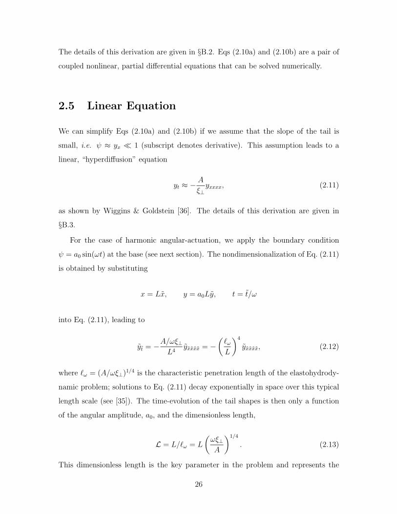
We can simplify Eqs (2.10a) and (2.10b) if we assume that the slope of the tail is

small, i.e. ψ ≈ yx " 1 (subscript denotes derivative). This assumption leads to a

linear, “hyperdiffusion” equation

yt ≈ −A

ξ⊥yxxxx, (2.11)

as shown by Wiggins & Goldstein [36]. The details of this derivation are given in

§B.3.

For the case of harmonic angular-actuation, we apply the boundary condition

ψ = a0 sin(ωt) at the base (see next section). The nondimensionalization of Eq. (2.11)

is obtained by substituting

x = Lx, y = a0Ly, t = t/ω

into Eq. (2.11), leading to

yt = −A/ωξ⊥L4

yxxxx = −(

,ω

L

)4

yxxxx, (2.12)

where ,ω = (A/ωξ⊥)1/4 is the characteristic penetration length of the elastohydrody-

namic problem; solutions to Eq. (2.11) decay exponentially in space over this typical

length scale (see [35]). The time-evolution of the tail shapes is then only a function

of the angular amplitude, a0, and the dimensionless length,

L = L/,ω = L

(ωξ⊥A

)1/4

. (2.13)

This dimensionless length is the key parameter in the problem and represents the

26

“floppiness” of the tail and hence the overall effectiveness of the swimmer. In partic-

ular, theory predicts an optimal dimensionless tail length as both short, stiff tails and

long, flexible tails produce negligible net translation—the first is ineffective owing to

the scallop theorem and the second owing to the excessive drag on the long passive

filament.

Using separation of variables, the solution to Eq. (2.11) can now be found to be

(see [35])

y(x, t) = a0,ω(eiωth(η), (2.14)

where η =x

,ωand h(η) =

4∑

j=1

cjeijz0η.

Here i is the imaginary number and the coefficients cj must be solved using the

boundary conditions of the problem, as discussed in the next section.

2.6 Boundary Conditions

In order to solve the equations of motion (Eqs 2.10a, 2.10b, and 2.11), we need to

apply boundary conditions. On examination of Eqs (2.10a) and (2.10b), we find that

there are four derivatives in the local angle, ψ, and two derivatives in the local tension,

τ . As a result, we must supply four boundary conditions for ψ and two more for τ .

For the linear equation, we have four derivatives in space and thus we supply four

boundary conditions.

In this thesis, we investigate a “fixed” swimmer where one end of the tail is

anchored and controlled in some manner; we call this the fixed end. The other end

of the tail is free to move in the fluid; we call this the free end. To see how this

applies to our equations of motion, let us revisit beam theory from undergraduate

solid mechanics. Physically, we can interpret the variables of our equations as shown

in Tbl. 2.1. Recall that subscripts denote derivatives and A = EI is the bending

stiffness, where E is the Young’s modulus of the material and I is the cross-section

moment of inertia. From beam theory, we know that the free end of the tail should be

27

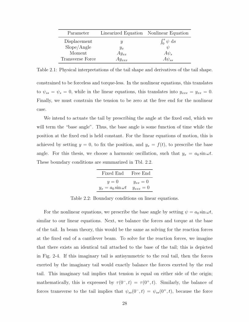
Parameter Linearized Equation Nonlinear Equation

Displacement y∫ s

0 ψ dsSlope/Angle yx ψ

Moment Ayxx Aψs

Transverse Force Ayxxx Aψss

Table 2.1: Physical interpretations of the tail shape and derivatives of the tail shape.

constrained to be forceless and torque-less. In the nonlinear equations, this translates

to ψss = ψs = 0, while in the linear equations, this translates into yxxx = yxx = 0.

Finally, we must constrain the tension to be zero at the free end for the nonlinear

case.

We intend to actuate the tail by prescribing the angle at the fixed end, which we

will term the “base angle”. Thus, the base angle is some function of time while the

position at the fixed end is held constant. For the linear equations of motion, this is

achieved by setting y = 0, to fix the position, and yx = f(t), to prescribe the base

angle. For this thesis, we choose a harmonic oscillation, such that yx = a0 sin ωt.

These boundary conditions are summarized in Tbl. 2.2.

Fixed End Free End

y = 0 yxx = 0yx = a0 sin ωt yxxx = 0

Table 2.2: Boundary conditions on linear equations.

For the nonlinear equations, we prescribe the base angle by setting ψ = a0 sin ωt,

similar to our linear equations. Next, we balance the forces and torque at the base

of the tail. In beam theory, this would be the same as solving for the reaction forces

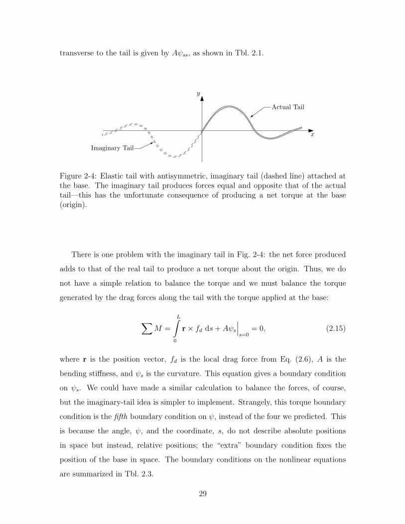
at the fixed end of a cantilever beam. To solve for the reaction forces, we imagine

that there exists an identical tail attached to the base of the tail; this is depicted

in Fig. 2-4. If this imaginary tail is antisymmetric to the real tail, then the forces

exerted by the imaginary tail would exactly balance the forces exerted by the real

tail. This imaginary tail implies that tension is equal on either side of the origin;

mathematically, this is expressed by τ(0−, t) = τ(0+, t). Similarly, the balance of

forces transverse to the tail implies that ψss(0−, t) = ψss(0+, t), because the force

28

transverse to the tail is given by Aψss, as shown in Tbl. 2.1.

y

x

Actual Tail

Imaginary Tail

Figure 2-4: Elastic tail with antisymmetric, imaginary tail (dashed line) attached atthe base. The imaginary tail produces forces equal and opposite that of the actualtail—this has the unfortunate consequence of producing a net torque at the base(origin).

There is one problem with the imaginary tail in Fig. 2-4: the net force produced

adds to that of the real tail to produce a net torque about the origin. Thus, we do

not have a simple relation to balance the torque and we must balance the torque

generated by the drag forces along the tail with the torque applied at the base:

∑M =

L∫

0

r× fd ds + Aψs

∣∣∣s=0

= 0, (2.15)

where r is the position vector, fd is the local drag force from Eq. (2.6), A is the

bending stiffness, and ψs is the curvature. This equation gives a boundary condition

on ψs. We could have made a similar calculation to balance the forces, of course,

but the imaginary-tail idea is simpler to implement. Strangely, this torque boundary

condition is the fifth boundary condition on ψ, instead of the four we predicted. This

is because the angle, ψ, and the coordinate, s, do not describe absolute positions

in space but instead, relative positions; the “extra” boundary condition fixes the

position of the base in space. The boundary conditions on the nonlinear equations

are summarized in Tbl. 2.3.

29

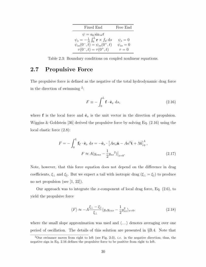
Fixed End Free End

ψ = a0 sin ωt

ψs = − 1A

∫ L

0 r× fd ds ψs = 0ψss(0−, t) = ψss(0+, t) ψss = 0

τ(0−, t) = τ(0+, t) τ = 0

Table 2.3: Boundary conditions on coupled nonlinear equations.

2.7 Propulsive Force

The propulsive force is defined as the negative of the total hydrodynamic drag force

in the direction of swimming 2:

F ≡ −∫ L

0

f · ex ds, (2.16)

where f is the local force and ex is the unit vector in the direction of propulsion.

Wiggins & Goldstein [36] derived the propulsive force by solving Eq. (2.16) using the

local elastic force (2.8):

F = −∫ L

0

fE · ex ds = −ex ·[Aκsn− Aκ2t + Λt

]L

0,

F ≈ A(yxxx −1

2yxx

2)∣∣x=0

. (2.17)

Note, however, that this force equation does not depend on the difference in drag

coefficients, ξ⊥ and ξ‖. But we expect a tail with isotropic drag (ξ⊥ = ξ‖) to produce

no net propulsion (see [1, 22]).

Our approach was to integrate the x-component of local drag force, Eq. (2.6), to

yield the propulsive force

〈F 〉 ≈ −Aξ⊥ − ξ‖

ξ⊥〈yxyxxx −

1

2y2

xx〉x=0, (2.18)

where the small slope approximation was used and 〈. . .〉 denotes averaging over one

period of oscillation. The details of this solution are presented in §B.4. Note that

2Our swimmer moves from right to left (see Fig. 2-3), i.e. in the negative direction; thus, thenegative sign in Eq. 2.16 defines the propulsive force to be positive from right to left.

30

Eq. (2.18) differs from Eq. (2.17) by a factor (ξ⊥ − ξ‖)/ξ⊥; this disparity arises from

a proper integration of the drag force on the filament [22].

When comparing experiments to theory, it is useful to define a nondimensional

propulsive force. Choosing the viscous penetration length, ,ω = (A/ωξ⊥)14 , as our

characteristic length we find

x = ,ωx, y = a0,ωy, t = T t,

where a0 is the angular amplitude, T is the period of oscillation, t is the dimensionless

time, and x and y are the nondimensional x and y, respectively. Substituting these

dimensionless parameters into Eq. (2.18), we find3:

〈F 〉 = Aξ⊥ − ξ‖

ξ⊥

1

T

(a0,ω)2

,4ω

T 〈yxyxxx −1

2y2

xx〉x=0

= (ξ⊥ − ξ‖)|ω|a20,

2ω〈yxyxxx −

1

2y2

xx〉x=0,

= a20,

2ω(ξ⊥ − ξ‖)|ω|〈F〉. (2.19)

It follows that the nondimensional force is

〈F〉 =〈F 〉

a20,

2ω(ξ⊥ − ξ‖)|ω|

. (2.20)

The above equation is valid for all F even though it was derived using the linear

expression for propulsive force.

3The 1/T comes from 〈. . .〉 = 1T (

∫ T0 . . . dt) and T comes from dt = T dt

31

32

Chapter 3

Methods and Implementation

To test the flexible oar theory presented in Chapter 2, we built a robotic swimmer;

this swimmer is described in §3.1 followed by a description of the experimental setup.

Section 3.3 describes how we measured the propulsive force generated by the swimmer.

This is followed by a description of how tail shapes were captured and compared to

theoretical tail shapes in §3.4. In §3.5, we describe the numerical solution of the

nonlinear equations. Finally, we conclude with a short section dealing with the wall

effects in our experiments.

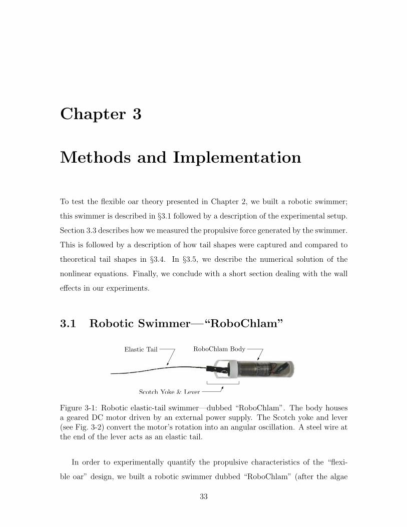
3.1 Robotic Swimmer—“RoboChlam”

Scotch Yoke & Lever

Elastic Tail RoboChlam Body

Figure 3-1: Robotic elastic-tail swimmer—dubbed “RoboChlam”. The body housesa geared DC motor driven by an external power supply. The Scotch yoke and lever(see Fig. 3-2) convert the motor’s rotation into an angular oscillation. A steel wire atthe end of the lever acts as an elastic tail.

In order to experimentally quantify the propulsive characteristics of the “flexi-

ble oar” design, we built a robotic swimmer dubbed “RoboChlam” (after the algae

33

Chlamydomonas), as is displayed in Fig. 3-1. The RoboChlam body was approxi-

mately 8 cm in length and housed a Nidec Copal HG-16-240-AA geared DC motor.

The motor’s rotation was converted into an angular oscillation; consequently, the

tail was angularly-actuated: the base of the filament was fixed at the origin and the

base-angle was varied sinusoidally with an amplitude a0 and a frequency ω. The

voltage across the motor was supplied by a laboratory power supply and governed

the oscillation frequency. The length of the lever, as shown in Fig. 3-2, controlled the

amplitude of oscillation, and at the end of the lever, stainless steel wires of various

lengths acted as elastic tails.

The rotation of the motor was converted to an angular oscillation using a combi-

nation of two mechanisms: a Scotch yoke and a lever. The Scotch yoke was made up

of the rotor, rotor pin, and follower shown in Fig. 3-2(a). As the rotor rotates at a

constant rate, the rotor pin traces out a circular motion. The pin moves the follower,

which is constrained to remain vertical (see Fig. 3-2b). Since the follower is basically

a vertical slot, whose width matches the diameter of the pin, the follower extracts the

horizontal component of the pin’s circular motion and “ignores” the vertical compo-

nent. Thus, the horizontal position of the follower varied sinusoidally. The follower

was connected to the lever by the follower pin, such that horizontal movement of

the pin produced rotation of the lever about the pivot (see Fig. 3-2c). Thus, for a

constant motor rotation rate, the mechanism produced an angular oscillation that

was approximately sinusoidal1.

3.2 Fixed Swimmer Experiment

RoboChlam was immersed in high viscosity silicone oil (polydimethylsiloxane, trimethyl-

siloxy terminated) to simulate the low Reynolds numbers experienced by micro-

organisms. A cantilever beam anchored RoboChlam (see Fig. 3-3), and a pair of

1Given the distance from the pivot to the follower pin L0, the radius of the circle traced outby the rotor pin r0, and the motor-rotation rate ω, the angle of the lever is expressed as α =arcsin( r0

L0sinωt), which is exactly sinusoidal when r0/L0 → 0. Note, geometric constraints require

r0/L0 ≤ 1.

34

ω

Rotor

Follower

Lever

PivotRotor

Motor

Tail

(a) (b) front view

(c) top view

Follower Pin

Rotor Pin

Figure 3-2: Scotch yoke and lever mechanism. The rotor and follower form theScotch yoke, which converts the motor’s rotation into a translational oscillation. Alever converts this translational oscillation into an angular oscillation.

strain gages on opposite sides of the beam measured beam deflection. Strain gage

readings were converted into force measurements. A video camera captured video

of the tail shapes generated by RoboChlam. Finally, videos of the tail shapes were

digitized for comparison to our simulations and theoretical predictions.

StrainGages

CantileverBeam

20 cm

35 cm

51 cm

VideoCamera

RoboChlam

Figure 3-3: Schematic of experimental setup to measure tail shapes and the propulsiveforce of the elastic tail.

3.3 Propulsive Force Measurement

In order to measure the propulsive force of our swimmer, a cantilever beam with strain

gages served as a force transducer. As shown, in Fig. 3-3, RoboChlam was mounted

at the free end of the cantilever beam. The thrust generated by the swimmer exerted

35

a force on the tip of the beam and deflected the beam. Strain gages mounted near

the base of the cantilever beam measured the deflection as an electrical signal. The

voltage output from the strain gages was processed using a Wheatstone bridge and

two amplifiers. The resulting signal was then fed to a computer where the strain

measurement was converted into a force measurement.

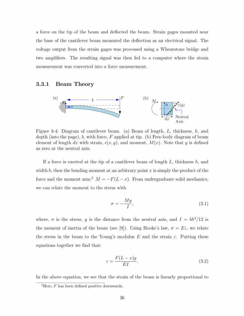
3.3.1 Beam Theory

FL

ε(y)xy

(a) (b)M

dx

h

NeutralAxis

Figure 3-4: Diagram of cantilever beam. (a) Beam of length, L, thickness, h, anddepth (into the page), b, with force, F applied at tip. (b) Free-body diagram of beamelement of length dx with strain, ε(x, y), and moment, M(x). Note that y is definedas zero at the neutral axis.

If a force is exerted at the tip of a cantilever beam of length L, thickness h, and

width b, then the bending moment at an arbitrary point x is simply the product of the

force and the moment arm:2 M = −F (L− x). From undergraduate solid mechanics,

we can relate the moment to the stress with

σ = −My

I, (3.1)

where, σ is the stress, y is the distance from the neutral axis, and I = bh3/12 is

the moment of inertia of the beam (see [9]). Using Hooke’s law, σ = Eε, we relate

the stress in the beam to the Young’s modulus E and the strain ε. Putting these

equations together we find that:

ε =F (L− x)y

EI. (3.2)

In the above equation, we see that the strain of the beam is linearly proportional to

2Here, F has been defined positive downwards.

36

the force at the tip. Also note that the force at the tip can be amplified by using a

long, thin beam and choosing a material with a low Young’s modulus.

In our experiment, two strain gages were mounted at equal distances d from the

base, but on opposite surfaces, y = h/2 and y = −h/2. As a result, the bending

strain measured from these gages will be equal and opposite in sign.

3.3.2 Strain Gages

Strain gages are used to transform the strain in the cantilever beam into an electri-

cal signal. Strain gages are essentially resistors that change resistance as they are

stretched or compressed. The relationship between the resistance of the gages and

the applied strain is given bydR

R= GFε, (3.3)

where GF is a constant of proportionality known as the gage factor, ε is the strain,

and R is the nominal (undeformed) resistance of the strain gage (see [12]).

3.3.3 Wheatstone Bridge Circuit

To measure the change in resistance of the strain gages, we used a circuit known as

a Wheatstone bridge (see Fig. 3-5). This bridge circuit is commonly used with strain

gages, as they provide a means to zero the voltage and are ideal for temperature

compensation. The relationship between the input voltage, Vin, and the output,

V1 − V2, can be shown (see [12]) to be

V1 − V2 = Vin

[R1R4 −R2R3

(R1 + R2)(R3 + R4)

]= Vout,0, (3.4)

where we have defined Vout,0 to be the voltage output when there is no load on the

beam, i.e. the strain gages are at their nominal resistances.

For the fixed swimmer experiment, the resistors R2 and R4 were chosen to equal

the nominal resistances for the strain gages3 R1 and R3 and from Eq. (3.4) we see

3In reality, R4 was a potentiometer with variable resistance, but was very close to R2 in resistance.

37

R3

R5

Vin

Strain Gages

−+

−+

R4

Wheatstone Bridge Differential Amplifier Inverting Amplifier

R1

R2

V1

V2

V3

VDAQ

R5

R6

R6

R7

R8

Figure 3-5: Diagram of circuit for strain gage measurement. The strain gages formtwo legs of the Wheatstone bridge whose output is amplified by two voltage amplifiers.The amplified signal is then sent to data acquisition equipment.

that the no-load voltage Vout,0 = 0. However, the resistances of the strain gages vary

with beam deflection, so we take the derivative of Eq. (3.4) with respect to R1 and

R3 to find

Vout = Vin

[R1R2

(R1 + R2)2

(dR1

R1

)+

R3R4

(R3 + R4)2

(− dR3

R3

)]. (3.5)

Now recall from §3.3.1 that the strain on the strain gages is of equal and opposite

magnitude so that dR1 = − dR3 = dR and define R = R1 = R2 = R3 = R4 so that

Eq. (3.5) becomes

Vout = Vin

[1

4

dR

R+

1

4

dR

R

]= Vin

dR

2R. (3.6)

Thus the strain readings from the two gages sum and provide a slight amplification.

Finally, we note that dR1 = − dR3 is only true for bending; for uniaxial tension or

thermal expansion, dR1 = dR3 and from Eq. (3.5) we find there is no change in

voltage output under these conditions.

3.3.4 Voltage Amplifiers

Although the force generated by the swimmer was modestly amplified by choosing a

long cantilever beam and using two strain gages, further amplification was required.

Because the output from the Wheatstone bridge, Vout, was actually a voltage differ-

38

ence, V1 − V2, the first amplification process used a differential amplifier, while the

second used an inverting amplifier. For the differential amplifier in Fig. 3-5, it can be

shown (see [12]) that

V3 =R6

R5(V1 − V2) =

R6

R5Vout. (3.7)

Similarly an inverting amplifer produces an output

VDAQ = −R8

R7V3. (3.8)

Now we can combine Eqs (3.2), (3.3), (3.6), (3.7), and (3.8) to find:

VDAQ = −R8

R7

R6

R5Vin

GF

2

F (L− d)h2

EI= −Vin

GF

2

R6R8

R5R7

(L− d)h2

EIF, (3.9)

recalling that the strain gages were positioned at y1 = h/2, y2 = −h/2, and x1,2 = d.

Since we want to determine the propulsive force of our swimmer given an input

voltage, we rearrange the above equation to find

F = −CNV VDAQ, (3.10)

where CNV =2

VinGF

R5R7

R6R8

EI

(L− d)h2

. (3.11)

Thus, the conversion from Volts to Newtons is constant if the values on the right-hand

side of Eq. (3.11) are constant.

3.3.5 Procedure for Force Measurement

A laboratory stand fixed one end of a thin beam made from DuPontTMDelrin R©.

Omega R©SG-6/120-LY13 strain gages were attached on opposite sides of the beam,

equidistant from the fixed end. RoboChlam was then attached to the opposite end

of the beam (free end), which held the swimmer in the silicone oil (see Fig. 3-3). The

strain gages were attached to the strain gage circuit and the output from the circuit

was attached to a National InstrumentsTMBNC-2110 terminal block allowing the volt-

age output to be acquired by a personal computer. MATLAB R©’s data acquisition

39

toolbox was used to view the electrical signal produced by the strain gage circuit.

The potentiometer on the Wheatstone bridge was adjusted until the voltage reading

was nearly zero. Finally, RoboChlam was turned on for 2–10 periods of oscillation

and the voltage at discrete increments of time (1/400 to 1/1500 s) was saved to file.

Tail Tail Young’s Moment BendingLength Diameter Modulus of Inertia StiffnessL[m] D[mm] E[GPa] I [m4]× 1015 A [N · m2]× 103

0.18–0.3 0.51 & 0.61 190 3.3 & 6.8 0.62 & 1.3

Table 3.1: Tail parameters for fixed RoboChlam.

Fluid Oscillation Angular ReynoldsViscosity Frequency Amplitude Numberµ[Pa · s] ω[rad/s] a0[rad] Re

3.18 0.4–5 0.814 & 0.435 10−2–10−3

Table 3.2: Experimental parameters for fixed RoboChlam.

Experiments showed that an angular oscillation starting with the tail at rest

reached steady-state motion after approximately two periods of oscillation; this decay

of transients was confirmed in our nonlinear simulations. Although force measure-

ments required deflection of the cantilever beam, this deflection was less than half

a centimeter at the beam’s tip and thus, RoboChlam’s position was approximately

fixed. It was also observed that the oscillation of the tail produced an oscillatory tor-

sion on the cantilever beam. Although a large beam width was chosen to reduce this

effect, it was not completely eliminated. Since any prismatic (polygonal cross-section)

beam under torsion will exhibit an axial strain [9], care had to be taken to eliminate

this strain from our measurements. Thus, the configuration of the Wheatstone bridge

and placement of strain gages were chosen to eliminate the effects of axial strain (see

§3.3.3).

A sample trial of the raw voltage data is shown in Fig. A-1. Note that the raw data

has zero-load readings at the beginning and end of the trial. This gave a quantitative

measurement of the drift in the no-load voltage and was used as a measurement of

40

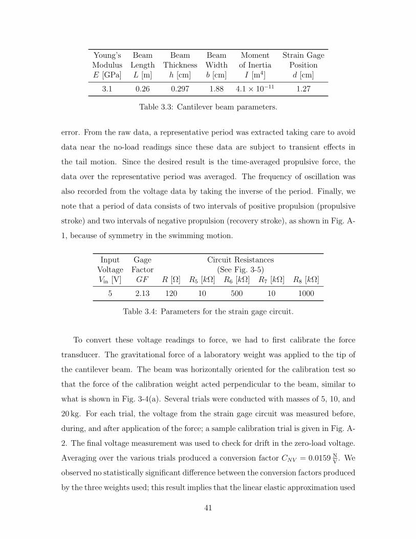
Young’s Beam Beam Beam Moment Strain GageModulus Length Thickness Width of Inertia PositionE [GPa] L [m] h [cm] b [cm] I [m4] d [cm]

3.1 0.26 0.297 1.88 4.1× 10−11 1.27

Table 3.3: Cantilever beam parameters.

error. From the raw data, a representative period was extracted taking care to avoid

data near the no-load readings since these data are subject to transient effects in

the tail motion. Since the desired result is the time-averaged propulsive force, the

data over the representative period was averaged. The frequency of oscillation was

also recorded from the voltage data by taking the inverse of the period. Finally, we

note that a period of data consists of two intervals of positive propulsion (propulsive

stroke) and two intervals of negative propulsion (recovery stroke), as shown in Fig. A-

1, because of symmetry in the swimming motion.

Input Gage Circuit ResistancesVoltage Factor (See Fig. 3-5)Vin [V] GF R [Ω] R5 [kΩ] R6 [kΩ] R7 [kΩ] R8 [kΩ]

5 2.13 120 10 500 10 1000

Table 3.4: Parameters for the strain gage circuit.

To convert these voltage readings to force, we had to first calibrate the force

transducer. The gravitational force of a laboratory weight was applied to the tip of

the cantilever beam. The beam was horizontally oriented for the calibration test so

that the force of the calibration weight acted perpendicular to the beam, similar to

what is shown in Fig. 3-4(a). Several trials were conducted with masses of 5, 10, and

20 kg. For each trial, the voltage from the strain gage circuit was measured before,

during, and after application of the force; a sample calibration trial is given in Fig. A-

2. The final voltage measurement was used to check for drift in the zero-load voltage.

Averaging over the various trials produced a conversion factor CNV = 0.0159 NV . We

observed no statistically significant difference between the conversion factors produced

by the three weights used; this result implies that the linear elastic approximation used

41

in §3.3.1 was valid and viscoelastic effects of the plastic beam were negligible4. The

time-averaged force was then found using Eq. (3.10). If we use the equation derived

earlier for CNV (Eq. 3.11) and the values from Tbls 3.3 and 3.4 instead of calibration

measurements, we find CNV = 0.013 NV . For all experimental data presented, the

calibrated CNV was used.

3.4 Tail Shape (Waveform) Comparison

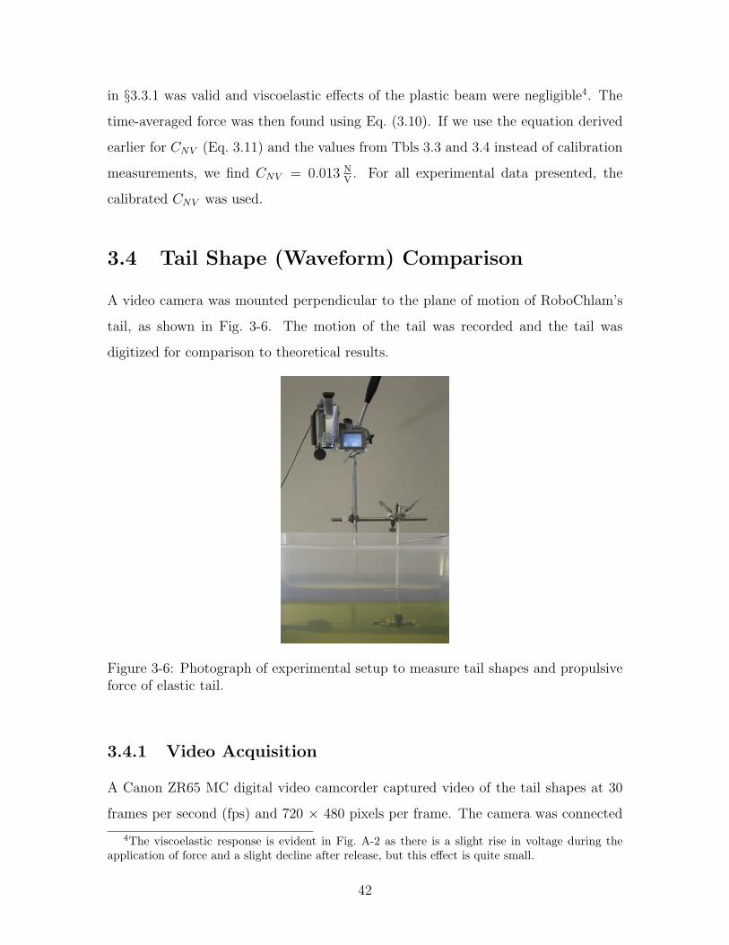
A video camera was mounted perpendicular to the plane of motion of RoboChlam’s

tail, as shown in Fig. 3-6. The motion of the tail was recorded and the tail was

digitized for comparison to theoretical results.

Figure 3-6: Photograph of experimental setup to measure tail shapes and propulsiveforce of elastic tail.

3.4.1 Video Acquisition

A Canon ZR65 MC digital video camcorder captured video of the tail shapes at 30

frames per second (fps) and 720 × 480 pixels per frame. The camera was connected

4The viscoelastic response is evident in Fig. A-2 as there is a slight rise in voltage during theapplication of force and a slight decline after release, but this effect is quite small.

42

by firewire to a personal computer running Windows XP, and WinDV was used to

record video in DV-AVI type 2 format. The camera’s focal plane was aligned with the

tail’s plane of motion, and the tail was centered in the frame. To eliminate transient

effects, RoboChlam was turned on for a minimum of two periods of oscillation; after

this time, a period of tail motion was recorded.

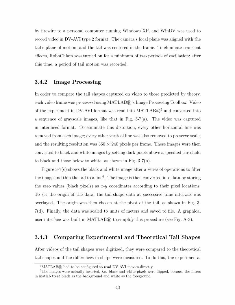
3.4.2 Image Processing

In order to compare the tail shapes captured on video to those predicted by theory,

each video frame was processed using MATLAB R©’s Image Processing Toolbox. Video

of the experiment in DV-AVI format was read into MATLAB R©5 and converted into

a sequence of grayscale images, like that in Fig. 3-7(a). The video was captured

in interlaced format. To eliminate this distortion, every other horizontal line was

removed from each image; every other vertical line was also removed to preserve scale,

and the resulting resolution was 360 × 240 pixels per frame. These images were then

converted to black and white images by setting dark pixels above a specified threshold

to black and those below to white, as shown in Fig. 3-7(b).

Figure 3-7(c) shows the black and white image after a series of operations to filter

the image and thin the tail to a line6. The image is then converted into data by storing

the zero values (black pixels) as x-y coordinates according to their pixel locations.

To set the origin of the data, the tail-shape data at successive time intervals was

overlayed. The origin was then chosen at the pivot of the tail, as shown in Fig. 3-

7(d). Finally, the data was scaled to units of meters and saved to file. A graphical

user interface was built in MATLAB R© to simplify this procedure (see Fig. A-3).

3.4.3 Comparing Experimental and Theoretical Tail Shapes

After videos of the tail shapes were digitized, they were compared to the theoretical

tail shapes and the differences in shape were measured. To do this, the experimental

5MATLAB R© had to be configured to read DV-AVI movies directly.6The images were actually inverted, i.e. black and white pixels were flipped, because the filters

in matlab treat black as the background and white as the foreground.

43

(a) Grayscale image from video. (b) Black and white image after threshold-ing grayscale image.

(c) Black and white image after filtering op-erations.

(d) Overlay of tail shape data at successivetime intervals.

Figure 3-7: Processed images of tail shapes.

tail data had to be aligned and synchronized with those from the linear and non-

linear theories. A graphical user interface was built in MATLAB R© to simplify this

procedure (see Fig. A-4).

Video capture was synchronized with the tail motion by eye, so the tail position

of the initial frame was unpredictable and had to be synchronized. Using the user

interface, the digitized tail was plotted on top of the theoretical tails (linear and

nonlinear). Slight adjustments were made in the digitized tail to account for offsets

in the vertical position and rotational orientation. After that, the initial frame of the

theoretical tails was adjusted to achieve the best alignment between the digitized tail

and the theoretical ones. The linear and nonlinear tail equations were solved at time

intervals equal to one fourth the time interval between video frames, i.e. 120 fps, to

increase the accuracy of the alignment.

44

x

y

∆x

∆yn

Figure 3-8: Schematic of two tails of different shapes. The difference in shape hasbeen exaggerated for clarity. A line connects each tail-tip and the vertical distance∆y was measured at 100 equally spaced points along the tail.

To get a quantitative measurement of the difference between tails, we first found

the difference in y-position between tails at 100 equally spaced points in the x-

direction, where ∆x = L/100 and L is the tail length. Note that the nonlinear

and experimental tails extend to x = L only when they are undeformed and exactly

horizontal; on the other hand, the linear tail always extends to x = L because of

the small deformation approximation. To account for differences in length along x,

a line is extended from the tip of the “shorter” tail to the tip of “longer” one before

finding the tail differences, as shown in Fig. 3-8. Note that this idealized tip region

contributed upwards of 10% of the difference measurement.

To complete this difference measurement, we use the Euclidean norm, given as

‖y‖ =

√√√√100∑

n=1

yn2. (3.12)

For a nondimensional difference we divide this norm by the tail length and the number

of points

D =‖y‖100L

. (3.13)

3.5 Numerical Solution of Nonlinear Equations

The nonlinear equations of motion (Eqs 2.10a and 2.10b) were solved numerically

using a Newton-Raphson iteration, also known as Newton’s method. What follows

45

is a brief description of this method with an example of how it was applied to the

nonlinear equations.

3.5.1 Newton’s Method of Root-Finding

y

xx0 x0 + ∆x

dfdx

f(x0)

f(x0 + ∆x)desired root

Figure 3-9: Arbitrary function, f(x) near root. To find the root, we choose an initialpoint x0 and find the slope df/ dx at that point. By extending a line with slopedf/ dx to the x-axis, we march closer and closer to the root.

Suppose we are given some continuous function f(x), which we can differentiate

to give df/dx. Our goal is to find the point(s), xr, where f(xr) = 0; in other words,

we want the root(s) of f(x). We first choose an arbitrary point along the curve, x0.

Assuming f(x) has a root and f(x0) /= 0 (otherwise, we need to look no further),

there is some ∆x for which

0 = f(xr) ≈ f(x0 + ∆x). (3.14)

We can approximate Eq. (3.14) using the first two terms of the Taylor series expansion:

f(x0) +df

dx

∣∣x0

∆x ≈ 0

Solving for ∆x, we have

∆x =−f(x0)

df/dx|x0

. (3.15)

We can see from Fig. 3-9, that f(x0 + ∆x) /= 0, but this new point is closer to zero7.

We then iterate, to find the desired zero.

7It will not always be the case that f(x0 + ∆x) is closer to zero than f(x0) – this has to do withthe stability of this root-finding method (see Hamming [14]).

46

The algorithm is summarized below.

1. Given f(x), find df/dx.

2. Choose a starting point x0.

3. Calculate ∆x =−f(x0)

df/dx|x0

.

4. Calculate f(x0 + ∆x).

• If this is close enough to zero, DONE.

• Otherwise, let xnew0 = x0 + ∆x and start over from step 3.

Of course, the definition of “close enough” to zero depends on the problem and the

desired accuracy.

3.5.2 Finite Difference Equation

To demonstrate Newton’s method of root-finding, we take a simplified form of Eq. (2.10a):8

∂ψ/∂t = −(A/ξ⊥) ∂4ψ/∂s4. Before tackling this equation, we define φ ≡ ∂2ψ/∂s2

such that∂ψ

∂t= − A

ξ⊥

∂2

∂s2

(∂2ψ

∂s2

)= − A

ξ⊥

∂2φ

∂s2. (3.16)

y

xBody

∆s

i = 0

i = N

Figure 3-10: Discrete version of elastic tail. The tail is divided into N straightsegments of length ∆s. This allows derivatives to be approximated as differenceequations.

As with most numerical schemes, we must replace the continuous problem with

a discretized form. In Fig. 3-10, the smoothly-curving elastic tail (see Fig. 2-3) has

8Note, this simplified form is very similar to the linear equation of motion.

47

been replaced by N straight links of length ∆s. What we have not shown is that time

has also been divided into discrete time intervals, ∆t. Next, we rewrite Eq. (3.16) in

terms of finite differences at the nth time interval and the ith point along the tail:

ψn+1i − ψn

i

∆t= − A

ξ⊥

φn+1i+1 − 2φn+1

i + φn+1i−1

∆s2, (3.17)

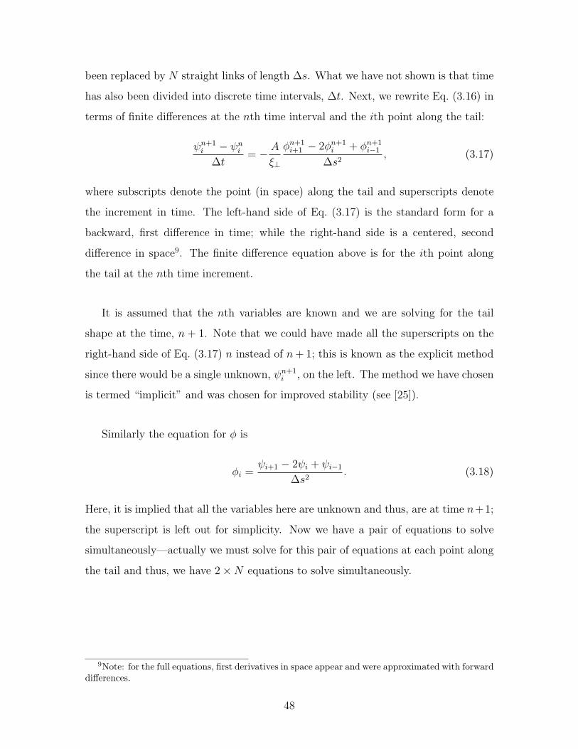
where subscripts denote the point (in space) along the tail and superscripts denote

the increment in time. The left-hand side of Eq. (3.17) is the standard form for a

backward, first difference in time; while the right-hand side is a centered, second

difference in space9. The finite difference equation above is for the ith point along

the tail at the nth time increment.

It is assumed that the nth variables are known and we are solving for the tail

shape at the time, n + 1. Note that we could have made all the superscripts on the

right-hand side of Eq. (3.17) n instead of n + 1; this is known as the explicit method

since there would be a single unknown, ψn+1i , on the left. The method we have chosen

is termed “implicit” and was chosen for improved stability (see [25]).

Similarly the equation for φ is

φi =ψi+1 − 2ψi + ψi−1

∆s2. (3.18)

Here, it is implied that all the variables here are unknown and thus, are at time n+1;

the superscript is left out for simplicity. Now we have a pair of equations to solve

simultaneously—actually we must solve for this pair of equations at each point along

the tail and thus, we have 2×N equations to solve simultaneously.

9Note: for the full equations, first derivatives in space appear and were approximated with forwarddifferences.

48

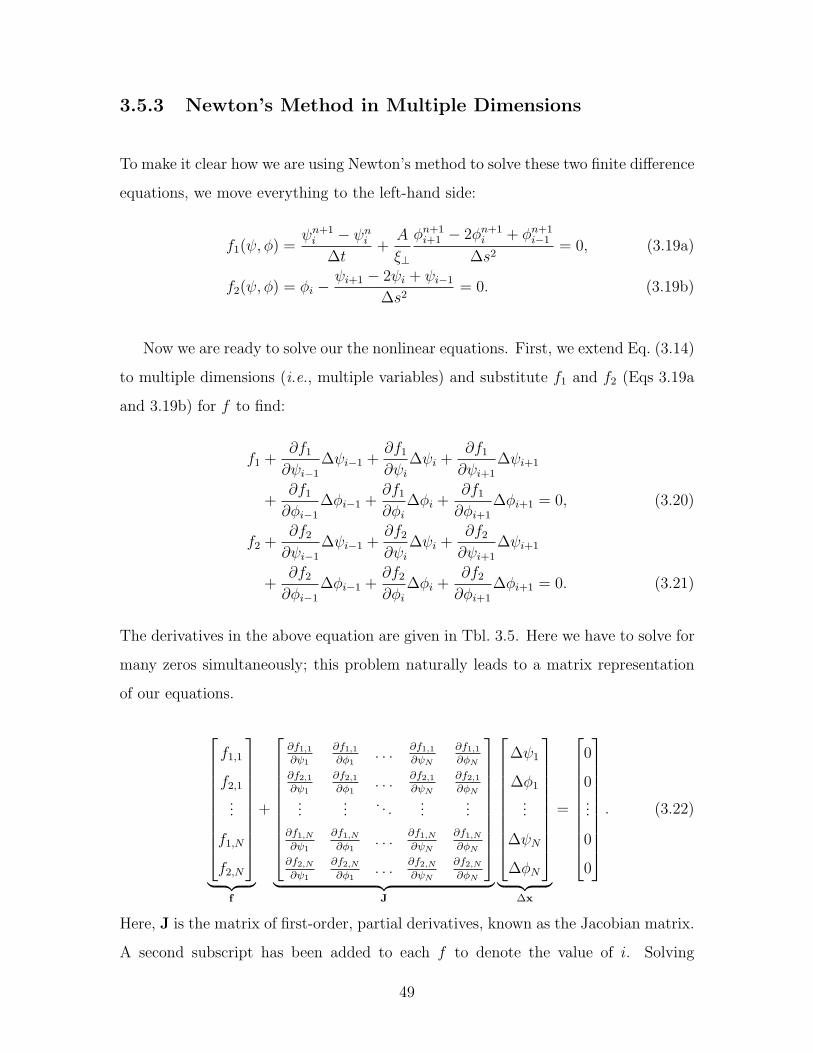
3.5.3 Newton’s Method in Multiple Dimensions

To make it clear how we are using Newton’s method to solve these two finite difference

equations, we move everything to the left-hand side:

f1(ψ, φ) =ψn+1

i − ψni

∆t+

A

ξ⊥

φn+1i+1 − 2φn+1

i + φn+1i−1

∆s2= 0, (3.19a)

f2(ψ, φ) = φi −ψi+1 − 2ψi + ψi−1

∆s2= 0. (3.19b)

Now we are ready to solve our the nonlinear equations. First, we extend Eq. (3.14)

to multiple dimensions (i.e., multiple variables) and substitute f1 and f2 (Eqs 3.19a

and 3.19b) for f to find:

f1 +∂f1

∂ψi−1∆ψi−1 +

∂f1

∂ψi∆ψi +

∂f1

∂ψi+1∆ψi+1

+∂f1

∂φi−1∆φi−1 +

∂f1

∂φi∆φi +

∂f1

∂φi+1∆φi+1 = 0, (3.20)

f2 +∂f2

∂ψi−1∆ψi−1 +

∂f2

∂ψi∆ψi +

∂f2

∂ψi+1∆ψi+1

+∂f2

∂φi−1∆φi−1 +

∂f2

∂φi∆φi +

∂f2

∂φi+1∆φi+1 = 0. (3.21)

The derivatives in the above equation are given in Tbl. 3.5. Here we have to solve for

many zeros simultaneously; this problem naturally leads to a matrix representation

of our equations.

f1,1

f2,1

...

f1,N

f2,N

︸ ︷︷ ︸f

+

∂f1,1

∂ψ1

∂f1,1

∂φ1. . . ∂f1,1

∂ψN

∂f1,1

∂φN

∂f2,1

∂ψ1

∂f2,1

∂φ1. . . ∂f2,1

∂ψN

∂f2,1

∂φN

......

. . ....

...∂f1,N

∂ψ1

∂f1,N

∂φ1. . . ∂f1,N

∂ψN

∂f1,N

∂φN

∂f2,N

∂ψ1

∂f2,N

∂φ1. . . ∂f2,N

∂ψN

∂f2,N

∂φN

︸ ︷︷ ︸J

∆ψ1

∆φ1

...

∆ψN

∆φN

︸ ︷︷ ︸∆x

=

0

0...

0

0

. (3.22)

Here, J is the matrix of first-order, partial derivatives, known as the Jacobian matrix.

A second subscript has been added to each f to denote the value of i. Solving

49

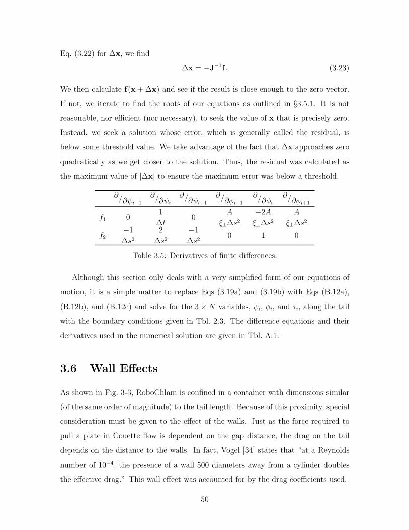
Eq. (3.22) for ∆x, we find

∆x = −J−1f . (3.23)

We then calculate f(x + ∆x) and see if the result is close enough to the zero vector.

If not, we iterate to find the roots of our equations as outlined in §3.5.1. It is not

reasonable, nor efficient (nor necessary), to seek the value of x that is precisely zero.

Instead, we seek a solution whose error, which is generally called the residual, is

below some threshold value. We take advantage of the fact that ∆x approaches zero

quadratically as we get closer to the solution. Thus, the residual was calculated as

the maximum value of |∆x| to ensure the maximum error was below a threshold.

∂/∂ψi−1∂/∂ψi

∂/∂ψi+1∂/∂φi−1

∂/∂φi∂/∂φi+1

f1 01

∆t0

A

ξ⊥∆s2

−2A

ξ⊥∆s2

A

ξ⊥∆s2

f2−1

∆s2

2

∆s2

−1

∆s20 1 0

Table 3.5: Derivatives of finite differences.

Although this section only deals with a very simplified form of our equations of

motion, it is a simple matter to replace Eqs (3.19a) and (3.19b) with Eqs (B.12a),

(B.12b), and (B.12c) and solve for the 3×N variables, ψi, φi, and τi, along the tail

with the boundary conditions given in Tbl. 2.3. The difference equations and their

derivatives used in the numerical solution are given in Tbl. A.1.

3.6 Wall Effects

As shown in Fig. 3-3, RoboChlam is confined in a container with dimensions similar

(of the same order of magnitude) to the tail length. Because of this proximity, special

consideration must be given to the effect of the walls. Just as the force required to

pull a plate in Couette flow is dependent on the gap distance, the drag on the tail

depends on the distance to the walls. In fact, Vogel [34] states that “at a Reynolds

number of 10−4, the presence of a wall 500 diameters away from a cylinder doubles

the effective drag.” This wall effect was accounted for by the drag coefficients used.

50

The drag coefficients given in Eqs (2.5a) and (2.5b) are derived for a slender cylin-

der in an infinite, unbounded fluid. There exists a wealth of drag-coefficient equations

to account for wall effects (compilations of these coefficients are given in [4, 30]). In

choosing the drag coefficients for this experiment, we used the experimental results of

Stalnaker and Hussey [30] that found best agreement with the drag coefficients from

de Mestre and Russel [10]. We present them here without derivation:

ξ⊥ =

∫ +l

−l

−8πµε

2 + εln(1− x2/l2) + 1− E⊥+ O(ε3)dx, (3.24)

ξ‖ =

∫ +l

−l

8πµε

4 + ε2 ln(1− x2/l2)− 2− E‖+ O(ε3)dx, (3.25)

where

E⊥ = arcsinh

(1 + x

2d

)+ arcsinh

(l − x

2d

)+

2(l + x)

(l + x)2 + 4d21/2

+2(l − x)

(l − x)2 + 4d21/2− (l + x)3

2(l + x)2 + 4d23/2− (l − x)3

2(l − x)2 + 4d23/2

and

E‖ =2 arcsinh

(1 + x

2d

)+ 2 arcsinh

(l − x

2d

)+

(l + x)

(l + x)2 + 4d21/2

+(l − x)

(l − x)2 + 4d21/2− 2(l + x)3

(l + x)2 + 4d23/2− 2(l − x)3

(l − x)2 + 4d23/2.

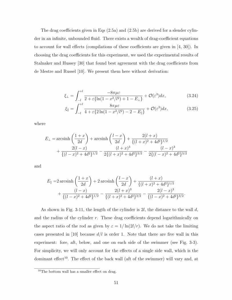
As shown in Fig. 3-11, the length of the cylinder is 2l, the distance to the wall d,

and the radius of the cylinder r. These drag coefficients depend logarithmically on

the aspect ratio of the rod as given by ε = 1/ ln(2l/r). We do not take the limiting

cases presented in [10] because d/l is order 1. Note that there are five wall in this

experiment: fore, aft, below, and one on each side of the swimmer (see Fig. 3-3).

For simplicity, we will only account for the effects of a single side wall, which is the

dominant effect10. The effect of the back wall (aft of the swimmer) will vary and, at

10The bottom wall has a smaller effect on drag.

51

x, ξ‖

y, ξ⊥

d

l l

2r

Figure 3-11: Schematic of slender rod of length 2l and a distance d from the wall.

times, dominates because we are using tails of different length so that the distance to

the back wall varies. For our experiments, the distance to the side wall d is taken to

be constant for simplicity, although this distance varies as the tail oscillates.

52

Chapter 4

Results and Discussion

The results of our investigations are summarized in Figs 4-1, 4-2 and 4-3. We first

display in Fig. 4-1 the propulsive force generated for a range of dimensionless tail

lengths, L. All parameters of the experiment were known or measured, and no fit-

ting of data was necessary. Figure 4-2 shows a comparison of the linear, nonlinear,

and experimental tail shapes while Fig. 4-3 gives a quantitative measurement of the

difference in tail shapes as a function of nondimensional length.

4.1 Propulsive Force

As shown in Fig. 4-1, agreement of the propulsive force with the theoretical (linear

model, Eq. 2.11) and numerical values (nonlinear model, Eqs. 2.10a and 2.10b) is

excellent. The force data from the RoboChlam experiments show a maximum di-

mensionless force at L = 2.14, in agreement with prediction from the theory. Note

that our data was nondimensionalized with the drag difference, ξ⊥−ξ‖ (see Eq. 2.20),

instead of the transverse drag ξ⊥, which was used in [36, 35]. The drag difference

originated in Eq. (2.18), and it represents the correct scaling as a tail with isotropic

drag (ξ⊥ = ξ‖) should produce zero propulsive force [1, 22]. We note also that the

maximum value of L that could be tested was limited by the motor’s rotation rate

and the length of tail that would fit in the experimental apparatus.

In comparing the data to linear elastohydrodynamic theories, there are three pri-

53

0

0.2

0.4

0.6

0.8

Non

dim

ensi

onal

Forc

e,F

Non

dim

ensi

onal

Forc

e,F

0 1 2 3 4 5Nondimensional Length, LNondimensional Length, L

linearnonlinearL = 18 cmL = 18 cmL = 20 cmL = 23 cmL = 30 cm

Figure 4-1: Force measurements for various tail lengths, L. Oscillation frequencywas varied to span range of dimensionless length, L. + has D = 0.61 mm anda0 = 0.814 rad. All other data have D = 0.5 mm and a0 = 0.435 rad.

mary sources of error: thermal drift in the experiment, wall effects, and the neglected

nonlinearities in the theory. The error bars in Fig. 4-1 arise from uncertainty in the

no-load voltage of the strain gage measurements. At lower oscillation frequencies, the

sample time of the experiment increased, leading to noticeable thermal drift in strain

gage (force) measurements and thus, larger drift error for the left-most points of a

given data-set.

Recall that the wall-correction to the drag coefficients only accounts for a single

side-wall of the tank, not the back wall, as is appropriate for all but the longest tails

in our experiments. The tip of the longest tail (30 cm, !) was only a few centimeters

from the back wall and thus, this wall had a non-negligible effect on the drag of the

longest tail resulting in an increased thrust as expected. For this tail, it seems logical

to use drag coefficients corrected for the effects of this dominant wall. However,

the orientation of the tail with respect to the back wall would produce coefficients

that vary along the length of the tail; we choose to avoid this complication in our

analysis. It is interesting to note that, in these experiments, nonlinear effects are

completely negligible relative to the other two sources of error even for long tails and

large actuation angles.

54

This analysis of the propulsive force would not be complete without a comparison

to biological micro-swimmers. For this comparison, we take a typical tail length

L = 60 µm and oscillation frequency ω = 135 rad/s for bull sperm [4]. For a slender

rod in water, we find a drag difference of ξ⊥ − ξ‖ ≈ 1× 10−3 Pa · s. If we assume an

optimized swimmer, we have F = 0.48 and L = 2.14 such that ,ω = L/L = 28 µm and

take a reasonable amplitude of a0 = 0.8 rad, we find that Eq. (2.20) gives F = 67 pN.

For comparison, bull sperm have measured propulsive forces of ∼ 250 pN [29]. This

discrepancy in force arises from the fact that RoboChlam is a passive-tail swimmer

with torque generated at the base, while sperm is an active-tail swimmer, producing

torque along the length of its tail.

4.2 Tail Shapes

(c)

(b)

(a)

−0.020

0.02−0.05

0

0.05

−0.05

0

0.05

y[m

]y

[m]

0 0.05 0.1 0.15 0.2

x [m]x [m]

linear nonlinear experiment

Figure 4-2: Comparison of three tail shapes for a tail with L = 20 cm, D = 0.5 mm,a0 = 0.435 rad, and oscillation frequencies (a) ω = 0.50 rad/s ( L = 1.73), (b) ω =1.31 rad/s (L = 2.20), (c) ω = 5.24 rad/s (L = 3.11).

In Fig. 4-2, we plot the tail shapes from experiments along with simulations from

55

both the linear and nonlinear theories. The plot shows three tails from a single data

set (constant L, D, and a0, but varying ω) with dimensionless lengths (a) L = 1.73,

(b) L = 2.20, and (c) L = 3.11. These dimensionless lengths span the region near the

maximum dimensionless force. The tail shapes from experiment matched well with

those from the linear and nonlinear simulations, and only slight differences between

the three tails were observed. Tails whose dimensionless length was small (Fig. 4-2a)

moved stiffly, while those with large dimensionless lengths (Fig. 4-2c) were flexible,

as predicted by theory. The difference between the different tail shapes (theory,

experiments, simulations) is quantified in Fig. 4-3. The measured errors are observed

to be small. The fact that the data match the linear simulation better than the

nonlinear solution is fortuitous and merely reflects the fact that resistive force theory

is only an approximation of the full hydrodynamic equations [20].

0

0.002

0.004

0.006

Tail

Diff

eren

ceTa

ilD

iffer

ence

1.5 2 2.5 3 3.5Nondimensional Length, LNondimensional Length, L

L-N, 1L-E, 1N-E, 1

L-N, 2L-E, 2N-E, 2

Figure 4-3: Normalized, time-averaged difference between linear (L), nonlinear (N),and experimental (E) tail shapes. The difference is calculated using Eq. (3.13). Twodata sets are shown: (1) L = 20 cm, D = 0.5 mm, and a0 = 0.435 rad; (2) L = 18 cm,D = 0.63 mm, and a0 = 0.814 rad.

56

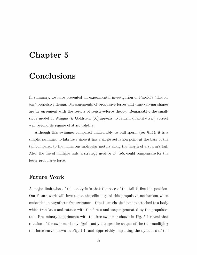
Chapter 5

Conclusions

In summary, we have presented an experimental investigation of Purcell’s “flexible

oar” propulsive design. Measurements of propulsive forces and time-varying shapes

are in agreement with the results of resistive-force theory. Remarkably, the small-

slope model of Wiggins & Goldstein [36] appears to remain quantitatively correct

well beyond its regime of strict validity.

Although this swimmer compared unfavorably to bull sperm (see §4.1), it is a

simpler swimmer to fabricate since it has a single actuation point at the base of the

tail compared to the numerous molecular motors along the length of a sperm’s tail.

Also, the use of multiple tails, a strategy used by E. coli, could compensate for the

lower propulsive force.

Future Work

A major limitation of this analysis is that the base of the tail is fixed in position.

Our future work will investigate the efficiency of this propulsive mechanism when

embedded in a synthetic free-swimmer—that is, an elastic filament attached to a body

which translates and rotates with the forces and torque generated by the propulsive

tail. Preliminary experiments with the free swimmer shown in Fig. 5-1 reveal that

rotation of the swimmer body significantly changes the shapes of the tail, modifying

the force curve shown in Fig. 4-1, and appreciably impacting the dynamics of the

57

swimmer. It is interesting to note that the large torque and transverse force generated

by the tail drag can be cancelled if we have two tails moving antisymmetrically, much

like the breast-stroke motion of Chlamydomonas.

SpeedControl

On/OffSwitch

Motor &Gearbox

Battery

8 cmFRONT VIEWSIDE VIEW

BalloonNeedle Valve

(a) (b)

Figure 5-1: Free-swimming RoboChlam. (a) Photograph of swimmer overlayed withthe tail-shape and body position extracted from the image. (b) Schematic showinghow the original RoboChlam has been encased in foam with a battery and simplecontrols.

As a final note and a suggestion for future work, the analysis presented herein as-

sumes a Newtonian fluid and a tail with a constant cross-section and uniform material

properties. Microorganisms in the body often swim in fluids that are non-Newtonian

and thus, it would be interesting to understand the effect of viscoelastic fluids on the

motion and propulsive force of an elastic tail. If we remove the second assumption

and allow for the cross-section to vary along the tail, the possible waveforms would

not be limited by the nondimensional length given in this thesis and this change could

produce a more effective swimmer.

58

Appendix A

Additional Figures and Tables

0 5 10 15-0.8

-0.7

-0.6

-0.5

-0.4

-0.3

-0.2

-0.1

0Strain Gauge Voltage

Time, [s]

Voltag

e,[V

]

Period

Figure A-1: Strain gage voltage curve proportional to the force generated by oscilla-tory tail motion. A period of motion has been isolated with an oscillation period of2.74 s. Note that this period contains two propulsive strokes (negative voltage peaks)and two recovery strokes (positive voltage peaks) because of symmetry in the swim-ming motion. A slight asymmetry in the two stokes is evident; this was likely causedby imperfections in the Scotch yoke mechanism and skewed placement in the tankleading to asymmetric wall effects. There is also a noticeable difference between theDC voltages before and after swimming; this is likely due to viscoelastic effects in thebeam and thermal drift in the circuitry.

59

0 2 4 6 8 10 12 14 16 18-10

-8

-6

-4

-2

0

2

4Conversion Factor = 0.015920 to 0.016187 [N/V]

Time, [s]

Vz = −7.242064 V

Vw = −1.080102 V

Vr = −7.140567 V

Voltag

e,[V

]

Figure A-2: Sample force calibration measurement using 10 gram weight at the endof the cantilever beam. Colored lines mark the range of data used to measure thevoltage of three regions: (1) the initial zero load region with average voltage Vz, (2)during weight application with voltage Vw, and (3) after weight release with voltageVr. Note the slight DC-voltage increase in region 2 and the slight decrease in region3; these are likely caused by viscoelastic effects in the beam, but are negligibly small.

60

Ter

mFin

ite

Diff

eren

ce∂f

∂ψ

n

∂f

∂φ

n

∂f

∂τ n

∂f

∂ψ

∂f

∂φ

∂f

∂τ

∂f

∂ψ

p

∂f

∂φ

p

∂f

∂τ p

ψt

ψ−

ψ0

dt

1 dt

A ξ ⊥ψ

ssss

A ξ ⊥

φp−

2φ+

φn

ds2

Aξ ⊥

ds2

−2A

ξ ⊥ds2

Aξ ⊥

ds2

−1 ξ ⊥

τψ

ss−

1 ξ ⊥τφ

−1 ξ ⊥

τ−

1 ξ ⊥φ

−B

τ sψ

s−

Bτ p−

τds

ψp−

ψds

B ds

τ p−

τds

B ds

ψp−

ψds

−B ds

τ p−

τds

−B ds

ψp−

ψds

−A ξ ‖

ψ2 sψ

ss−

A ξ ‖

(ψ

p−

ψds

) 2φ

2A

φξ ‖

ds

ψp−

ψds

−A ξ ‖

(ψ

p−

ψds

) 2−

2A

φξ ‖

ds

ψp−

ψds

φ−

ψss

φ−

ψp−

2ψ

+ψ

n

ds2

−1

ds2

2 ds2

1−

1ds2

τ ss

τ p−

2τ+

τ nds2

1 ds2

−2

ds2

1 ds2

Aψ

2 ssA

φ2

2Aφ

Cψ

sψ

sss

Cψ

p−

ψds

φp−

φds

−C ds

φp−

φds

−C ds

ψp−

ψds

C ds

φp−

φds

C ds

ψp−

ψds

−βτψ

2 s−

βτ

(ψ

p−

ψds

) 22βτ

ds

ψp−

ψds

−β

(ψ

p−

ψds

) 2−

2βτ

ds

ψp−

ψds

Tab

leA

.1:

Fin

ite

diff

eren

ces

and

thei

rder

ivat

ives

wher

eβ

=ξ ‖ ξ ⊥

,B

=1 ξ ⊥

+1 ξ ‖,an

dC

=A

(1+

β).

For

ψ,δ,

and

τ,su

bsc

ripts

nan

dp

den

ote

i−

1an

di+

1,re

spec

tive

ly(n

osu

bsc

ript

den

otes

i).

61

Figure A-3: Screenshot of user interface for video processing.

62

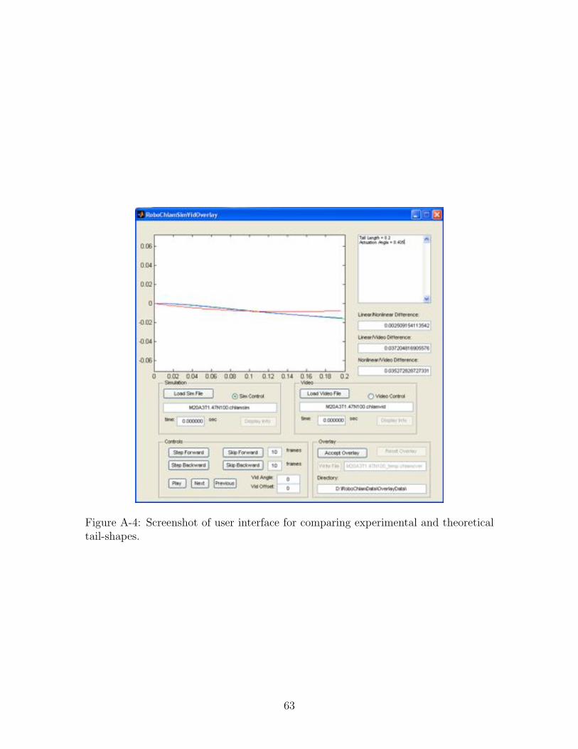
Figure A-4: Screenshot of user interface for comparing experimental and theoreticaltail-shapes.

63

64

Appendix B

Solution of Governing Equations

Derivations in §B.1 and §B.2 are similar to those found in Camalet and Julicher [5].

B.1 Elastic Force of Slender Rod

The elastic energy of the tail is given by Eq. (2.7) as

E =

∫ L

0

[A

2κ2 +

Λ

2rs

2

]ds.

The elastic force per unit length is fε = −δE/δr, where δ/δr is the first variation,

or functional derivative, with respect to the tail shape r, which is a function of the

arclength s (hence, functional derivative). Note that the curvature of the tail κ is a

function of the tail shape. Thus we take

δEδr

=

∫ L

0

δ

[A

2κ2 +

Λ

2rs

2

]ds =

∫ L

0

[Aκδκ + Λrs · δrs] ds.

The Frenet-Serret equations give

rs = t, (B.1a)

ts = κn = rss, (B.1b)

ns = −κt, (B.1c)

65

where subscripts denote derivatives. It follows that1

δκ = δ(n · rss)

= n · δrss + rssδn

= n · δrss. (B.2)

Now we substitute Eqs (B.1a) and (B.2) into the Eq. (B.1) to give

δEδr

=

∫ L

0

[Aκn · δrss + Λt · δrs

]ds. (B.3)

The goal is to make the integrand in Eq. (B.3) a function of the variation of r

and not its derivatives, rs or rss. First we integrate the first term in the integrand by

parts2

∫ L

0

[Aκn · δrss]ds = [Aκn · δrs]L0 −

L∫

0

[Aκsn + Aκ(−κt)] · δrsds.

Further integration by parts3 gives

∫ L

0

[Aκsn− Aκ2t)] · δrsds =[[Aκsn− Aκ2t]·δr

]L

0

−∫ L

0

∂s[Aκsn− Aκ2t] · δr ds.

(B.4)

The first term in the integrand has now been transformed into an integral with δr

in the integrand, plus four boundary terms. For the second term in the integrand of

Eq. (B.3), we integrate to find4:

∫ L

0

Λt · δrsds =[Λt · δr

]L

0−

∫ L

0

∂s[Λt] · δr ds. (B.5)

The sum of the integrands on the right-hand sides of Eqs (B.4) and (B.5) is the elastic

1Here we have used: rss = ts = κ · n so that rssδn = κn · δn = 0 (n and δn are orthogonal).2We let u = Aκn and dv = δrssds.3u = [Aκsn−Aκ2t] and dv = δrsds4u = Λt and dv = δrsds.

66

force5:

fε = −δEδr

= −∂s[Aκsn− Aκ2t + Λt]. (B.6)

The force in the tangential direction can be defined as the tension so that Eq. (B.6)

gives, Λ = −τ + Aκ2 [5], and we have

fε = −∂s[Aκsn− τ t]

= −Aκssn + Aκsκt + κτ n + τst

= −(Aκss − κτ)n + (Aκsκ + τs)t (B.7)

B.2 Nonlinear Equations of Motion

To solve for the equations of motion, recall Eq. (2.6) from resistive-force theory

fd = −[ξ⊥nn + ξ‖tt] · rt.

Since each segment of the tail is in equilibrium, the local drag force must be balanced

by the local elastic force, such that fd + fε = 0. Now substitute the drag force, fd, and

dot both sides by [(1/ξ⊥)nn + (1/ξ‖)tt] to find

rt =

(1

ξ⊥nn +

1

ξ‖tt

)· fε. (B.8)

If we substitute the elastic force, fε into the equation above, we get

rt =

(1

ξ⊥nn +

1

ξ‖tt

)·[−(Aκss − κτ)n + (Aκsκ + τs)t

],

= − 1

ξ⊥(Aψsss − ψsτ)n +

1

ξ‖(Aψssψs + τs)t, (B.9)

where κ = ψs.

From Eqs (B.1a) and (B.1b) it follows that ∂trs = nψt. Thus, the equation of

motion for ψ(s) is found by taking the spacial derivative of Eq. (B.9) and keeping

5δF =∫ (

δFδg(x)

)δg(x)dx.

67

only the n component so that

ψt = − 1

ξ⊥(−ψsτs + Aψssss − ψssτ) +

1

ξ‖(Aψssψs

2 + ψsτs). (B.10)

The above equation is the first equation of motion.

The second equation of motion is found by assuming that the elastica is incom-

pressible along its length so that it satisfies the constraint ∂trs2 = 2rs·∂trs = 2t·∂trs =

0. In other words, we take the derivative of Eq. (B.9) w.r.t. s and keep only the t

component to find

τss −ξ‖ξ⊥

ψs2τ = −

(1 +

ξ‖ξ⊥

)Aψsssψs − Aψss

2. (B.11)

In order to solve these nonlinear equations numerically, we rewrite Eqs (B.10) and

(B.11) as a system of second order partial differential equations:

f1 = ψt +1

ξ⊥(Aφss − τφ− τsψs)−

1

ξ‖

(Aψs

2φ + τsψs

)= 0, (B.12a)

f2 = φ− ψss = 0, (B.12b)

f3 = τss − βτψs2 + A

(1 +

ξ‖ξ⊥

)(ψsφs) + Aφ2 = 0. (B.12c)

B.3 Linear Equations of Motion

We will start with Eqs (B.6) and (B.8):

rt = −(

1

ξ⊥nn +

1

ξ‖tt

)· fε,

fε = −∂s[Aκsn− Aκ2t] = (−Aκss + Aκ3)n + 3Aκκst. (B.13)

Notice that the inextensibility constraint, Λ, does not appear in the elastic force

above because inextensibility is implied for small deformations. Combining these two

68

equations, we get:

rt =

(1

ξ⊥nn +

1

ξ‖tt

)· (−Aκss + Aκ3)n + 3Aκκst

=− 1

ξ⊥(Aκss − Aκ3)n +

1

ξ‖3Aκκst. (B.14)

From geometry, we know that

κ =dψ

ds=

yxx√1 + y2

x

≈ yxx, (B.15a)

n =1√

1 + y2x

−yx

1

≈

−yx

1

, (B.15b)

t =1√

1 + y2x

1

yx

≈

1

yx

. (B.15c)

The final step in the above equations assumes that the tail is undergoing small de-

formation and thus yx " 1. We can now rescale our equations, such that y = hy and

x = Lx, where h/L = ε and split the velocity into components so that rt = (xt, yt).

Thus,

xt =1

ξ⊥

(A

h

L4yxxxx − A

h3

L6y3

xx

)h

Lyx +

1

ξ‖3A

h2

L5yxxyxxx

=1

ξ⊥

(A

ε2

L3yxxxxyx − A

ε4

L4y3

xxyx

)+

1

ξ‖3A

ε2

L3yxxyxxx,

and

yt =− 1

ξ⊥

(A

h

L4yxxxx − A

h3

L6y3

xx

)− 1

ξ‖3A

h2

L5yxxyxxx

h

Lyx

=− 1

ξ⊥

(A

ε

L3yxxxx − A

ε3

L3y3

xx

)− 1

ξ‖3A

ε3

L3yxyxxyxxx.

69

where derivatives in s have become derivatives in x for small slopes. Eliminating

orders of ε greater than unity, we find that our linearized equations of motion are:

xt = 0,

yt = − 1

ξ⊥Ayxxxx. (B.16)

B.4 Linear Propulsive Force

The definition of the time average propulsive force is given by Eq. (2.16):

〈F 〉 ≡ − 1

T

∫ T

0

∫ L

0

f · ex ds dt, (B.17)

where T is the period of oscillation. The negative sign on the right-hand side of the

above equation appears because the propulsive direction is negative (see Fig. 2-3).

The hydrodynamic drag force given by Eq. (2.6) is:

fd = [ξ⊥nn + ξ‖tt] · rt,

where the free stream velocity u = 0. The local slope of the elastica is given by ψ(s),

such that the local unit normal and unit tangent can be expressed as

n =

sin ψ

− cos ψ

, t =

cos ψ

sin ψ

. (B.18)

The tensor products of these unit vectors become

nn =

sin2 ψ − sin ψ cos ψ

− sin ψ cos ψ cos2 ψ

, tt =

cos2 ψ sin ψ cos ψ

sin ψ cos ψ sin2 ψ

. (B.19)

For small angles we can approximate sinψ and cos ψ as

sin ψ ≈ yx, cos ψ ≈ 1 (B.20)

70

and we can let

rt =

xt

yt

≈

0

yt

, (B.21)

recalling that subscripts denote derivatives. Since we are only concerned with the x-

component of the force, we can take the x-component of Eq. (B.19) and also substitute

Eqs (B.20) and (B.21) to give

fx =

ξ⊥

yx2

−yx

+ ξ‖

1

yx

·

0

yt

(B.22)

= (ξ‖ − ξ⊥)yxyt. (B.23)

Note that the subscript of fx describes the x-component of local drag force and is

not a derivative. Pausing a moment to analyze the above equation, we see that the

local propulsive force is simply a product of the drag difference, the local slope, and

the vertical velocity. The above equation is exactly where physical arguments should

lead: for a nearly horizontal rod moving in the vertical direction, the transverse drag

would be large, but only a small component of the transverse drag (yxξ⊥) would act

in the x-direction. Similarly, a small component of the velocity (yxyt) is along the

axial direction.

If we substitute Eq. (2.11) into the equation above we get

fx = Aξ⊥ − ξ‖

ξ⊥yxyxxxx = A

ξ⊥ − ξ‖ξ⊥

[d

dx(yxyxxx)− (yxxyxxx)

](B.24)

= Aξ⊥ − ξ‖

ξ⊥

[d

dx(yxyxxx)−

d

dx

(1

2y2

xx

)]. (B.25)

Thus the propulsive force is

F =

∫ L

0

Aξ⊥ − ξ‖

ξ⊥

[d

dx(yxyxxx)−

d

dx

(1

2y2

xx

)]dx

= Aξ⊥ − ξ‖

ξ⊥

[yxyxxx −

1

2y2

xx

]

x=0

, (B.26)

recalling that yxx = yxxx = 0 at x = L as shown in Tbl. 2.2. Now we can substitute

71

this expression into Eq. (B.17)

〈F 〉 = −Aξ⊥ − ξ‖

ξ⊥

1

T

∫ T

0

[yxyxxx −

1

2y2

xx

]

x=0

dt. (B.27)

72

Bibliography

[1] L.E. Becker, S.A. Koehler, and H.A. Stone. On self-propulsion of micro-machines

at low reynolds number: Purcell’s three-link swimmer. Journal of Fluid Mechan-

ics, 490:15–35, 2003.

[2] H. C. Berg. E. coli in Motion. Springer-Verlag, NY, 2004.

[3] D. Bray. Cell Movements. Garland Publishing, New York, NY, 2000.

[4] C. Brennen and H. Winet. Fluid mechanics of propulsion by cilia and flagella.

Annual Review of Fluid Mechanics, 9:339–398, 1977.

[5] S. Camalet and F. Julicher. Generic aspects of axonemal beating. New Journal

of Physics, 2:1–23, 2000.

[6] Brian Chan. Propulsion devices for locomotion at low reynolds number. Master’s

thesis, Massachusetts Institute of Technology, 2004.

[7] S. Childress. Mechanics of Swimming and Flying. Cambridge Studies in Math-

ematical Biology. Cambridge University Press, Cambridge, 1st edition, 1981.

[8] R G Cox and S G Mason. Suspended Particles in Fluid Flow Through Tubes.

Annual Review of Fluid Mechanics, 3(1):291–316, 1971.

[9] Roy R. Craig. Mechanics of Materials. John Wiley & Sons, Inc., second edition,

2000.

[10] N. J. De Mestre and W. B. Russel. Low-reynolds-number translation of a slender

cylinder near a plane wall. Journal of Engineering Mathematics, 9:81–91, 1975.

73

[11] R. Dreyfus, J. Baudry, M. L. Roper, M. Fermigier, H. A. Stone, and J. Bibette.

Microscopic artificial swimmers. Nature, 437:862–865, 2005.

[12] Richard S. Figliola and Donald E. Beasley. Theory and Design for Mechanical

Measurements. John Wiley & Sons, Inc., third edition, 2000.

[13] J. Gray and G. J. Hancock. The propulsion of sea-urchin spermatozoa. J. Exp.

Biol., 32:802–814, 1955.

[14] R. W. Hamming. Numerical Methods for Scientists and Engineers. Dover Pub-

lications, 1973.

[15] M. Kim and T. R. Powers. Hydrodynamic interactions between rotating helices.

Physical Review E, 69(6):061910, June 2004.

[16] Y. W. Kim and R. R. Netz. Pumping fluids with periodically beating grafted

elastic filaments. Physical Review Letters, 96:158101, 2006.

[17] S. A. Koehler and T. R. Powers. Twirling Elastica: Kinks, Viscous Drag, and

Torsional Stress. Physical Review Letters, 85(22):4827–4830, 2000.

[18] M.C. Lagomarsino. Biologically Inspired Problems Concerning Semiflexible Fila-

ments. PhD thesis, FOM Institute for Atomic and Molecular Physics (AMOLF),

2004.

[19] Eric Lauga, Willow R. DiLuzio, George M. Whitesides, and Howard A. Stone.

Swimming in circles: Motion of bacteria near solid boundaries. Biophysical

Journal, 90:400, 2005.

[20] J. Lighthill. Flagellar hydrodynamics - The John von Neumann lecture, 1975.

SIAM Review, 18:161–230, 1976.

[21] James LIghthill. Mathematical Biofluiddynamics. SIAM, 1975.

[22] C. P. Lowe. Dynamics of filaments: modelling the dynamics of driven micro-

filaments. Philosophical Transactions of the Royal Society of London, Series

B-Biological Sciences, 358:1543–1550, 2003.

74

[23] K. E. Machin. Wave propagation along flagella. Journal of Experimental Biology,

35:796–806, 1958.

[24] K. E. Machin. The control and synchronization of flagellar movement. Proceed-

ings of the Royal Society, B, 158:88–104, 1963.

[25] William H. Press, Brian P. Flannery, Saul A. Teukolsky, and William T. Vet-

terling. Numerical Recipes in C : The Art of Scientific Computing. Cambridge

University Press, 1992.

[26] E. M. Purcell. Life at low reynolds number. American Journal of Physics, 45:3–

11, 1977.

[27] E. M. Purcell. The efficiency of propulsion by a rotating flagellum. Proceedings

of the National Academy of Sciences of the United States of America, 94:11307–

11311, 1997.

[28] M. Roper, R. Dreyfus, J. Baudry, M. Fermigier, J. Bibette, and H. A. Stone. On

the dynamics of magnetically driven elastic filaments. Journal of Fluid Mechan-

ics, 554:167–190, May 2006.

[29] Kathleen A. Schmitz, Dana L. Holcomb-Wygle, Danial J. Oberski, and

Charles B. Lindemann. Measurement of the Force Produced by an Intact Bull

Sperm Flagellum in Isometric Arrest and Estimation of the Dynein Stall Force.

Biophysical Journal, 79(1):468–478, 2000.

[30] John F. Stalnaker and R. G. Hussey. Wall effects on cylinder drag at low reynolds

number. Physics of Fluids, 22:603–613, 1979.

[31] Daniel Tam and A. E. Hosoi. Optimal stroke patterns for purcell’s three link

swimmer. Phys. Rev. Lett., In Review.

[32] G. I. Taylor. Analysis of the swimming of microscopic organisms. Proceedings of

the Royal Society, A, 209:447–461, 1951.

75

[33] G. I. Taylor. The action of waving cylindrical tails in propelling microscopic

organisms. Proceedings of the Royal Society, A, 211:225–239, 1952.

[34] S. Vogel. Life in Moving Fluids: The Physical Biology of Flow. Princeton Uni-

versity Press, 1994.

[35] C. H. Wiggins, D. Riveline, A. Ott, and R. E. Goldstein. Trapping and wiggling:

Elastohydrodynamics of driven microfilaments. Biophysical Journal, 74:1043–

1060, 1998.

[36] Chris H. Wiggins and Raymond E. Goldstein. Flexive and propulsive dynamics

of elastica at low reynolds number. Physical Review Letters, 80:3879–3882, 1998.

[37] C. W. Wolgemuth, T. R. Powers, and R. E. Goldstein. Twirling and whirling:

Viscous dynamics of rotating elastic filaments. Physical Review Letters, 84:1623–

1626, 2000.

76