1

Electricity Shortages and Firm Productivity:

Evidence from China’s Industrial Firms

Karen Fisher-Vanden, Erin T. Mansur, and Qiong (Juliana) Wang*

October 27, 2014 Unreliable inputs to production, particularly those that are difficult to store, can significantly limit firms’ productivity, leading them to react in a number of ways. This paper uses a panel of 23,000 energy-intensive, Chinese firms from 1999 to 2004 to examine how firms responded to severe power shortages in the early 2000s. Our results suggest that, in response to electricity scarcity, Chinese firms re-optimize among inputs to production by substituting materials for energy (both electric and non-electric sources)—a shift from “make” to “buy” of intermediate inputs to production. While outsourcing can be costly, Chinese firms were able to avoid substantial productivity losses by doing so. As a result of the increase in electricity scarcity from 1999 onward, we find that unit production costs increased by eight percent. JEL Codes: D24, Q4, P2, L9 Key Words: electricity, blackouts, productivity, China, outsourcing

* Fisher-Vanden: Dept of Agric. Econ. and Rural Soc., Pennsylvania State University 112-E Armsby Bldg, University Park, PA 16802, fishervanden@psu.edu; Mansur: Dartmouth College and NBER. Department of Economics, 6106 Rockefeller Hall, Hanover, NH 03755, erin.mansur@dartmouth.edu; Wang: Environmental Studies Program, University of Southern California, 3502 Trousdale Parkway, SOS B15, MC 0036, Los Angeles, CA 90089, juliana.wang@usc.edu. This research was supported by the U.S. Department of Energy’s Biological and Environmental Research Program (contract \#DE-FG02-04-ER63930), and the National Science Foundation (project/grant \#450823). We wish to thank Taryn Dinkelman, Eric Edmonds, Jun Ishii, Josh Linn, Nancy Rose, Connie Shang, and seminar participants at the UC Energy Institute, Harvard University, the ASSA meetings, and NBER for helpful comments.

2

1. Introduction

Resource availability and input factor reliability are important for firm

productivity, and are especially problematic in developing countries like China. For some

resources, like water, storage devices can be used to manage unreliable services (Baisa et

al. 2010). However, unreliable delivery of electricity requires that firms respond in other

ways, as power is prohibitively expensive to store.

Over the past few decades, investment in the Chinese power sector has

experienced a boom-bust cycle. Beginning in 1985, the central government transferred

ownership of power plants to local governments and firms. At first, this “privatization”

provided suppliers with an incentive to invest in new power capacity. In fact, the rapid

increase in new power plant construction during the 1990s lead to a glut of capacity (IEA

2006). In response, the national government imposed a building moratorium on new

power plants in 1999. As a result, within just a few years, this excess supply had

disappeared as demand quickly caught up with supply.

From 2000 to 2007, demand for electric power in China grew 41% (EIA 2009).

Most of this growth can be attributed to growth in the manufacturing sector, particularly

in construction-related products like steel and cement. By 2006, the manufacturing sector

comprised 74% of total electricity consumption (NBS 2007). In addition, while a smaller

overall share, household demand had been growing about 12% per year during this time

period. This was exacerbated by the fact that retail electricity remained under price-cap

regulation with limited price response to shortages. Finally, residential and commercial

electricity consumers were given priority over other customers, resulting in even less

electricity available for use by industrial sectors. Power availability and reliability were

3

further aggravated during the early 2000s by unusually hot summers and cold winters,

extreme weather events such as snow storms in the mid-South, and a shortage in coal

supply (Lin et al. 2005, Wang 2007). As a result, 26 of the 30 Chinese provinces

experienced blackouts associated with resource scarcity issues from 2002 to 2004 (Chen

and Jia 2006).

While the early 2000’s were historic in terms of the number of blackouts,

electricity shortages continue to remain a major concern for China. As recently as the

summer of 2011, China faced substantial power shortages.1 The severity of these

electricity shortages dwarfs recent experiences in the United States. In 2004, China’s

Eastern electricity grid (an area including Shanghai) alone curtailed over 13,000,000

MWh, accounting for over two percent of annual consumption. In comparison, the rolling

blackouts of California’s power crisis in 2000-2001 curtailed less than one 1000th of that

amount.2

In this paper, we apply econometric techniques to an unbalanced panel of firm-

level data comprising approximately 23,000 of the most energy-consuming firms in 11

industries in China from 1999 to 2004 to examine firm responses to the threat of

electricity shortages.3,4 In particular, we estimate a flexible cost function and test whether

1 Shanghai Securities News (http://english.cnstock.com/enghome/homeheadline/201105/1307904.htm (Accessed December 19, 2011)). 2 In 2004, Eastern China used 2.5 times as much electricity as California. Curtailment data are from China’s Eastern Grid Company (personal communication) and the California Public Utilities Commission (http://docs.cpuc.ca.gov/word\_pdf/misc/generation+report.pdf accessed June 20, 2008), respectively. Below we discuss how China’s electricity sector is made up of several transmission grids. 3 The data are by enterprise, which we refer to as a “firm” throughout this paper. In the data, an enterprise refers to a business organization but is not aggregated to the parent-company level. 4 As discussed in Section 4 below, we prefer to use a measure of electricity scarcity that captures the threat of scarcity, since firms will make investment decisions based on the potential threat of scarcity whether or not that particular firm has experienced a blackout. Thus, we use the ratio of thermal generation to capacity as our measure of threat.

4

input factor shares or overall productivity change with shocks to an electricity grid’s

degree of scarcity. We use weather data to instrument for potential measurement error

and endogeneity concerns.

Our results suggest that Chinese firms re-optimize in response to electricity

scarcity. Primarily, they shift from purchases of energy inputs (from both electric and

non-electric, primary energy sources) into material inputs. This is consistent with the

hypothesis of outsourcing: firms in regions where electric power became scarcer shift

from “make” to “buy” of intermediate goods for production. Further, we do not find

evidence that electricity scarcity led to an increase in self generation. This is in contrast to

findings from papers that study countries with long-term electricity supply issues (for

example, Allcott et al. 2014 for India), although the factors behind these shortages are

different.

Our results find that, across all industries, the increase in material inputs

expenditures in response to electricity shortages since 1999 increased unit production

costs by 13 percent. We find the largest effects in the wood products (e.g., furniture),

chemicals, food, metal, and textiles industries. However, this 13% increase in unit cost

due to greater spending on materials is partially offset by a 5% reduction in unit cost due

to savings in the other inputs and small total factor productivity improvements.

Therefore, the net effect of these factor-biased and factor-neutral effects is an 8%

increase in unit costs. Thus, while outsourcing can be costly, Chinese firms were able to

avoid substantial productivity losses by doing so since it led to savings elsewhere in the

production process.

5

This paper proceeds as follows. In Section 2, we describe the causes of and

regulatory response to China’s power shortage. Section 3 provides a discussion of

alternative ways that firms may respond to issues of electricity scarcity. Sections 4 and 5

describe our data and empirical model, respectively. In Section 6, we report our results.

We estimate the overall productivity losses attributable to the power shortages in Section

7, and conclude in Section 8.

2. Government Responses to Electricity Shortages

The Chinese government utilized both demand and supply side mechanisms in

response to the electricity shortages in the early 2000’s. On the demand side, some

dynamic pricing mechanisms were instituted to smooth the load between peak and off-

peak times. For example, Jiangsu province implemented time-of-use pricing starting in

2003. However, the effectiveness of this pricing policy was limited by regulatory control

on prices and the slow installation of real-time meters.

In addition, the government reduced subsidies for some industries. Since the mid-

1980s, the national government has subsidized purchased power for energy-intensive

industries including aluminum, cement, steel, and other metal and non-metal

manufacturing. The fertilizer and agriculture sectors are the most heavily subsidized

industries. In Junan Province, firms in these industries paid about a quarter the rate of

commercial users in 1999. Even during the crisis, these industries continued to receive

extremely low rates. However, for many industries, reduced subsidies and increased rates

began in 2002.

6

These pricing mechanisms, however, did not sufficiently curtail demand. As a

result, local governments were forced to address these shortages through either scheduled

blackouts (via quota rationing), or rolling, stochastic blackouts. Planned outages and

changes in production schedules were imposed to deal with the shortages. For example,

in the summer of 2003, the city of Hangzhou implemented a detailed plan for rolling

blackouts for industrial customers. These measures include: shifting firms with non-

continuous production to alternative working days (e.g., three-day per week production

schedules); controlling and cutting off electricity consumption at continuous production

firms during peak hours; moving energy-intensive production to night hours; limiting

power supply to key firms and projects; and lowering electricity consumption of

commercial users. The cities of Nanjing, Shanghai, and Shantou also released similar

plans during that period.

The Chinese government also implemented supply-side policies to expand

generation. The National Development and Reform Commission authorized the

construction of new power plants and the expansion of the grid system, all backed by

favorable financing packages offered through the state-owned banks. However, given the

long construction cycle, the effects of these supply-side efforts were not felt immediately.

The purpose of our analysis is to measure the response of Chinese firms to the

threat of electricity shortages. In Section 3, we account for these government demand and

supply market-based policies when discussing how firms might have responded to these

shortages. Namely, we are interested in the private industrial costs of electricity shortages

(or more generally, regulatory-induced scarcity) rather than the overall energy costs of

7

meeting demand growth. Presumably, these electricity shortages would not have occurred

in a free market, whereby prices could adjust to clear the market.

3. Firm Responses to Electricity Shortages

Electricity is the dominant source of energy in the manufacturing sector,

comprising more than 40% of primary energy consumption in the sector while coal is

approximately 25%. As a result, the manufacturing sector is extremely vulnerable to

shortages in electricity supply. Depending upon a firm’s ability to substitute to alternative

forms of energy, this reliance on electricity may result in manufacturing firms taking the

full brunt of electricity shortages. News reports suggested large economic costs as a result

of these electricity shortages. Many of these reports were based on isolated case studies

or surveys. For example, Zhejiang Province reported costs related to blackouts during

2004 to be 100 billion Yuan, or 9% of gross regional product.5 In estimating the cost of

blackouts in China, Lin et al. (2005) use data from a survey that asked firms their stated

willingness-to-pay to avoid an outage as well as their expenditures on backup generators.

The authors estimate the marginal cost of an hour of outage to be 78,482 Yuan, or

approximately USD$10,000.6

When facing electricity shortages, firms may respond in a number of ways. The

manner in which firms respond will depend, in part, on whether blackouts are planned

(i.e., scheduled rationing) or unanticipated (i.e., uncertain stochastic occurrences). For

example, if faced with power rationing, a firm might choose to invest in energy efficiency

5 Chinese Business Times (Dec. 12, 2004) http://finance.sina.com.cn/g/20041222/03001241424.shtml1. (Accessed April 14, 2007). The article does not explain how these estimates were calculated. 6 This working paper has been incorporated into Dong and Li (forthcoming).

8

improvements. This would only make sense if there were quota rationing in response to

electricity shortages. A second reason would be if regulators instituted policies promoting

energy efficiency at the regional level. In this case, the value share of capital would likely

increase while the shares of electricity and other energy inputs would fall. In contrast,

capital investments may be negatively affected if power shortages reduce capital

productivity or durability (Abeberese 2014).

Another common response to sustained power supply issues is for firms to invest

directly in technology in order to generate electricity on site, or “self generation.” In

addition to the required additional capital and diesel purchases, investment in self

generation will crowd out other investment opportunities, reducing productivity

(Reinikka and Svensson 2002).7

In the case of self generation, other types of energy are substitutes for purchased

electricity.8 This may particularly be true for industries at the top of the rolling blackouts

list. During these periods of shortages, many light industries, such as food processing or

textiles, were among the first to face electricity quotas. Many of these firms were

reported to be working only four days a week or working during off-peak hours (Natural

Resources Defense Council 2003, World Bank 2005, Thompson 2005). We expect that a

firm’s ability to respond by self generating may be limited in the short run. If firms

expected sustained electricity shortages in the future, they may be willing to make capital

investments that are potentially irreversible.

7 Alby, Detherier, and Straub (2011) find self-generation increases with power outages, using firm-level data from over 80 countries. Similarly, Reinikka and Svensson (2002) find that firms invest in their own power generators when Ugandan electric power supply is unreliable and inadequate. 8 Rosen and Houser (2007) and IEA (2006) reported that some firms and residents installed diesel-powered self-generation in response to the scarcity in China. This led to a 16% increase in oil demand in 2004, accounting for 27% of the increase in world oil demand that year.

9

Another option would be for the firm to outsource the production of energy-

intensive, intermediate goods rather than to produce them in-house.9 Firms may decide to

purchase intermediate goods rather than produce these goods from raw materials. In this

case, materials would be a substitute for electricity. In addition, outsourcing could result

in less use of labor, capital, and other energy sources in the production of these

intermediate goods. For example, a firm requiring steel as an input to production may

either purchase the raw inputs (e.g., pig iron, coal and electricity) to manufacture steel on

site, or the firm may decide to purchase the steel from other producers, especially if

electricity is unreliable. In this case, as these other inputs are no longer needed due to

outsourcing, these inputs would be complements of electricity. Compared to self

generation which could be a reasonable long-run response to sustained shortages, out-

sourcing could be a reasonable short-term response to electricity shortages.

Any of these three responses may lead to losses in productivity. In addition, if

changing inputs is too costly in the short-run, then firms may experience losses in

productivity due to reduced output. Also, extra costs may be incurred due to the need to

re-arrange production schedules. Jyoti, Ozbafli, and Jenkins (2006) note that a common

measure of the economic cost of blackouts is to calculate the loss in value added or in

contribution (net revenue) resulting from firm-level measures of actual outage durations.

These costs include labor costs, material spoilage costs, and restarting costs.

On the other hand, necessity may be the mother of invention. Firms may find

ways to become more productive when resources become scarce. For example,

9 This relates to literatures on supply-chain management (de Kok and Graves 2003) and on second sourcing in the face of uncertainty (Dick 1992).

10

Borenstein and Farrell (2007) find that firms in the US gold industry exhibit x-

inefficiencies, which can survive in industries with barriers to entry.

In contrast to the literature, this paper examines how the threat of electricity

shortages affects productivity in an immense and rapidly-growing economy, namely

China. Using firm-level panel data, we study how firms respond to electricity shortages

and estimate the resulting lost productivity.

Four testable hypotheses of how firms may respond to electricity shortages emerge from

the discussion above:

I. Decreased Productivity: firms may have limited options to respond, implying

that electricity shortages may increase unit costs.

II. Self Generation: firms may self generate, substituting away from electricity

toward non-electric energy and capital.

III. Outsourcing: firms may outsource more and produce less in-house, implying

more material use and less use of the other factors of production.

IV. Energy Efficiency: firms may invest in more energy efficiency technologies, for

example in response to quota rationing, reducing use of both types of energy and

increasing capital inputs.

4. Data

We test these hypotheses using a data set comprising of firm-level information on

production, electricity, self generation of electricity, and out-sourcing of material inputs.

11

Details on the sources of these data and the construction of key variables are provided

below.

Production Data

Our empirical estimation requires firm-level production data on capital, labor,

energy, and materials inputs and production costs. We construct this data set by merging

two firm-level data sets. The first is a set of economic and financial survey data, collected

by the National Bureau of Statistics (NBS) in China, comprising primarily large and

medium firms based on sales revenue for the years 1999-2004. A second data set, also

collected by the NBS for the same years, comprises information on annual energy use,

both in values and physical quantities, by approximately 20 energy types. From 1999 to

2003, the data are for the largest energy-consuming firms. Notably, the last year of our

sample was a census year where we have information on energy use for most medium

and large firms. We also utilize industry-level data from the Chinese national accounts to

construct industry-level prices of materials.

When we combine these data, we are left with an unbalanced sample of 36,943

observations from 22,902 different firms.10 As these data sets comprise repeated cross-

sections of survey data (and are thus a sample of the full population of firms), the set of

firms included in the data set changes each year and does not necessarily include the

same firms over time. The annual sample ranges from approximately 2900 in the year

2000 to about 19,000 firms in the census year, 2004 (see Panel B of Table 1). Most firms 10 In the analysis below, we focus on the industrial response to electricity shortages for firms using electricity as an input. Therefore we exclude firms in the electricity generation industry (4095 observations). We exclude observations missing control variables (10,272 observations), as well as those with potential reporting errors on input prices (1274 outliers). Most of these missing variables are input prices of capital, electricity, non-electricity energy, or materials. For the outliers, we truncate at 0.5% and 99.5% of the distribution for each reported input price.

12

report in only one year (16,899 firms), with the 2004 census year accounting for most of

these observations (15,215). Our analysis controls for firm fixed effects. Therefore, as

discussed below, the remaining 6,003 firms that report in more than one year help

identify the parameters of interest.

Panel A of Table 1 summarizes the number of firms reporting for a specific

number of years—that is, there are 16,899 firms reporting in only one year while there

are 731 firms reporting in all six years. Thus, if we were to use a balanced sample from

1999 to 2004, we would be estimating based on information for 731 firms only. If we

were to limit the sample to observations starting in 2000 or 2001, the balanced sample

would be comprised of 898 or 1310 firms, respectively. We therefore choose to estimate

our empirical model on the unbalanced sample.

A natural concern that arises with an unbalanced sample is sample selection bias.

The unbalanced nature of our data set is primarily due to two factors. First, in the 2004

census, we observe about half of our sample (15,215) for the first time because of their

relatively low energy use. The second factor is the sampling thresholds during the other

years: the economic and financial data set comprises only firms with sales revenue in

excess of five million yuan (approximately $600,000) and the energy data set comprises

only firms that consume energy in excess of 10,000 tons standard coal equivalent (SCE).

There is little actual entry of new firms, or exit of existing ones in these data sets due to

the focus on large firms (Fisher-Vanden and Jefferson 2008). Rather, during the 1999-

2003 survey years, firms near the sample cut off—either for energy use or total sales—

are entering and exiting the sample. As these data are not random samples, our results are

13

descriptive of a sample of Chinese firms that are above these thresholds for total annual

sales and total annual energy use. The importance of measuring the energy bias of

electricity scarcity requires us to work with the smaller, less representative sample.

Nonetheless, we test the robustness of our results by estimating our empirical model

using the balanced samples mentioned above (see Appendix Table A1). A related

concern is that the large number of mid-sized firms in 2004 drive the main results (that

we test in Table A2).11 We explore this in our robustness tests below.

While not comprehensive, our data set comprises the largest energy-consuming

firms in China. Since the energy sample criterion is based on levels and not intensity of

energy consumed, the sample includes both energy intensive firms (firms with a higher

energy/sales ratio) and firms that may be less energy intensive, but are large enough to

consume more than 10,000 tons SCE of energy. These firms cover almost 60 percent of

industrial energy use, 40 percent of sales, a third of employment, and a fifth of total

assets (see Appendix Table A3). The data include firms of various private and public

ownership structures. Most energy-intensive firms in capital-intensive sectors are state-

owned in China. State-owned firms account for 62 percent of our data. As discussed

further in Section 6 and shown in Appendix Table A4, as a robustness check, we examine

whether ownership affects how firms responded to electricity shortages.

We use the combined data to explore substitution patterns across inputs beyond

just capital and labor. We separate energy consumption into electricity and non-electricity

11 As mentioned above, about half of the observations in our sample are for the year 2004. Since 2004 is a census year, we have energy information for almost all medium and large firms in this year—thus, there are firms in our unbalanced sample that only show up in the year 2004. The sample of year 2004 observations differ from other year samples in that firms that use less energy show up in 2004 but not in other years; e.g., the 2003 and 2004 samples have similar distributions for the value of goods sold and value added, but not for energy.

14

energy (primarily coal and oil) and include five factor inputs in our model of production

cost: labor, capital, materials, electricity, and non-electricity energy sources. Using our

firm-level panel data set, we compute prices for each of the five inputs by firm and by

year based on expenditures. Thus, the price of labor is the sum of the wage bill and

welfare payments, divided by total employees. The price of capital, or fixed assets, is

imputed from total value added minus total labor expenses, divided by net value fixed

assets. The price of non-electricity energy is calculated as total other energy expenditures

divided by the quantity of energy purchased in standard coal equivalent (SCE) units. The

electricity price is similarly defined. In order to compute the price of materials, we use

data on industrial prices by year from the China Statistical Yearbook (CSY) published by

the National Bureau of Statistics. We compute the price of materials for a given firm in a

specific industry as a composite of annual industry prices weighted by input-output

shares for that firm’s industry. Thus, firms within the same two-digit Standard Industrial

Classification (SIC) industry face the same materials prices over time—i.e., these prices

vary annually for each of the 37 SIC categories. In an analysis with firm fixed effects,

changes in prices of non-electricity energy will reflect changes in the composition of the

bundle of energy inputs into each of these categories.

Table 2 reports the summary statistics for total costs, sales revenue, factor prices

and factor shares for our sample. The table reveals substantial variation in firm size. The

cost of goods sold, the dependent variable in the analysis, has a mean of 446 million

Yuan (approximately $50 million) with a standard deviation of 1556 million Yuan

(approximately $190 million). The ratio of the standard deviation to the mean (the

coefficient of variation) is quite large for sales revenue (the gross value of industrial

15

output in constant prices) and input prices (with the exception of the price of materials),

suggesting large variation in sales and input prices across firms. The large range that we

observe for several input prices suggests that some outliers remain, even after truncating

the sample (see footnote 10). Therefore, in the analysis below, we use the natural log of

all these cost and sales variables to smooth out this heterogeneity and curtail the effect of

outliers (Wooldridge 2006).

Table 2 also reports the summary statistics for the input value shares in our

sample. The materials costs account for about two thirds of all costs for the median

observation. Capital costs are about a sixth, followed by labor, electricity and other

energy costs. The table shows substantial variation in these shares across observations.

In order to better understand the heterogeneity across industries in our sample,

Table 3 reports the average factor value shares across all years in our sample for mining,

food, textiles, wood products, petroleum products, chemicals, rubber, non-metal mineral

products, metal products, machinery, and other industries. This table also includes firms

in the electric power industry for comparison purposes only as they are not used in the

analysis below. While the NBS classifies firms into 37 two-digit SIC categories, some

have insufficient observations to estimate the effects by industry. Therefore, this table

reflects the aggregation of two-digit SIC industries that will be used in our industry-

specific estimation.

Table 3 shows that the most energy-intensive industries include petroleum

processing and coking, non-metal products, chemicals, and other industries. In contrast,

the food and beverage and the machinery industries spend five percent or less of their

costs on energy. All industries use electricity and will be both directly and indirectly

16

affected by electricity shortages. While there is not a perfect placebo test, we examine

two possible candidates. First, we test whether industries that use less electricity were

less sensitive to the electricity shortages. The industries with the lowest electricity shares

are petroleum, machinery, and food. Second, as discussed further in Section 6, we

examine a set of firms across many industries that are likely to be less energy intensive

and therefore less affected by power shortages.

Electricity Data

Our estimation method, described in Section 5, requires an electricity scarcity

measure. China had six main regional grids in 2002—Central, East, North, Northeast,

Northwest, and South—each encompassing several provinces.12 Power is transmitted

with relative ease within a grid but has limited capability across grids. There are a

number of potential electricity scarcity measures that could be considered for use in our

analysis. First, we could use high-frequency (e.g., hourly) data on blackouts for each firm

in our sample. Second, we could use regional (i.e., grid-level) high-frequency data and

estimate the empirical distribution of the likelihood of blackouts. Third, we could proxy

for this empirical distribution of the likelihood of blackouts in each region by using

summary statistics (e.g., mean, variance, and deciles based on the hourly data).

Each of these measures can be problematic and thus which measure of electricity

scarcity is appropriate to use in our analysis is dependent on the question we are posing.

Although we would prefer to use a measure related to (2), such data are not available.

Thus, we adopt a version of (3)—in particular, the ratio of thermal electricity generated to

12 Grid systems in Xizang (Tibet) and Taiwan are not connected with China’s national grid system and are not included in our data.

17

thermal electricity capacity—as our measure of scarcity for reasons summarized below.

We also conduct tests on alternative scarcity measures.

Firm-level, high-frequency data on the duration of each blackout period would

seem ideal for our analysis. Much of the literature on the cost of blackouts, like Jyoti,

Ozbafli, and Jenkins (2006), use this type of measure. However, there are several reasons

why an alternative measure would be preferred in our context. Data on blackouts are

limited. However, even if these data were available, using blackouts as our measure of

scarcity raises the concern that provincial regulators may allocate the limited electricity to

the most productive firms. By aggregating across firms within a region, we use a measure

that does not suffer from this particular concern.

It is also important to consider whether a measure of blackouts is the appropriate

measure to use given our research question. We are most interested in firms’ responses to

the threat of electricity shortages, whether or not actual blackouts occurred. Focusing

only on firms that have actually experienced a blackout would cause us to miss the large

number of firms that are making investments or modifications to their production process

to hedge against the risk of a blackout. Most firms will not wait until a blackout occurs to

take risk avoiding measures. The ratio of generation to capacity is a good measure of the

potential for blackouts, as the potential of blackouts is larger the closer this ratio is to one.

Lastly, it seems that our measure of scarcity would likely be correlated with blackouts.

For the Eastern Grid only, we have additional data on the length and quantity of

electricity interruptions. The correlation between the annual MWh curtailed and our main

18

scarcity measure is 0.41, suggesting that our measure of scarcity is a decent proxy for the

duration of blackouts.13

Grid level performance indicators like capacity factors (e.g., generation/capacity)

are a meaningful way to measure the extent of power system reliability, or scarcity,

within a region. Within each grid, the transmission of power is frequent and with minimal

congestion. However, in the absence of long distance transmission direct current lines,

the transfer of electric power across grids has been difficult. As a result, in tight markets,

provinces are able to provide power to other provinces located within the same regional

grid through load management, but the sharing of power across grids to meet peak

demand is, in most cases, impossible. Thus, the capacity factor of a specific regional grid

is a decent indicator of the potential for electric power shortages within the region.

We use data on electricity scarcity constructed from information obtained from

various issues of the China Electricity Yearbook. These Yearbooks contain information

on electricity generation (𝐺𝐺𝐺𝑔𝑔𝑇ℎ𝑒𝑒𝑒𝑒𝑒) and capacity (𝐶𝐶𝐶𝑔𝑔𝑇ℎ𝑒𝑒𝑒𝑒𝑒) from thermal

(primarily coal-fired) power plants. Our main measure of scarcity is the thermal capacity

factor for grid g in year t: 𝑆𝑔𝑔𝑇ℎ𝑒𝑒𝑒𝑒𝑒 = 𝐺𝐺𝐺𝑔𝑔𝑇ℎ𝑒𝑒𝑒𝑒𝑒/𝐶𝐶𝐶𝑔𝑔𝑇ℎ𝑒𝑒𝑒𝑒𝑒, although we test

alternative capacity measures in our analysis.14

13 The correlation between annual curtailment and aggregate consumption is very high, 0.9. This may indicate that some new capacity may not have been available in the reported year. 14 For Figure 1, we adjust this variable for the number of hours in a year and account for power plant outages. Power plants typically schedule outages for maintenance and reliability purposes, sor. In addition, unscheduled outages occur due to equipment failure, for. Thus, we measure the expected annual capacity by multiplying capacity, which is in megawatts (MW) or MW-hours per hour, by (number of hours in a year)*(1-sor-for). In the econometric analysis, we take the natural logarithm of this variable so these multiplicative adjustments do not affect the estimation. The measures of sor and for are based on thermal generators of at least 100 MW (China Electricity Yearbook, 2000). If we had power plant outage measures that varied by space and time, then this adjustment formula would be important to include in the estimation.

19

The annual average thermal capacity factor by grid is provided in Figure 1.15

This figure shows greater scarcity in the North and East grids, and increasing scarcity in

all grids over time. In the analysis below, we include year-industry and firm fixed effects.

Therefore, identification of the overall effects of scarcity requires that the general upward

trend in scarcity varies by region. To test this, we regress a grid’s annual scarcity on grid

and year fixed effects. The overall fit has an R-squared of 0.91 for our sample period,

suggesting that some variation remains to identify the main results.16

This scarcity measure has the potential to reflect the overall likelihood of

blackouts in a given year, which is likely to be relevant for the medium-term labor hiring,

capital investment, and outsourcing decisions that we see in our firm-level productivity

data. However, we considered alternative capacity factors as our measure of scarcity as

well. One alternative measure is based on the single hour of a year when blackouts are

most likely to occur. This is measured by the ratio of annual peak electricity consumption

(MW) within a grid over total capacity: 𝑆𝑔𝑔𝑃𝑒𝑒𝑃 = 𝐶𝑃𝑃𝑃𝑃𝑃𝑃𝑃𝑔𝑔𝑇𝑇𝑔𝑒𝑒/𝐶𝐶𝐶𝑔𝑔𝑇𝑇𝑔𝑒𝑒, where total

capacity also includes nuclear and hydropower (see Figure A2 in the Appendix).17 This

measure focuses on the highest demand hour only and may be less informative of the

overall probability of blackouts throughout the year. The correlation between this

measure of scarcity and our preferred measure is 0.45. We also considered a scarcity

measure of the ratio of total generation over total capacity: 𝑆𝑔𝑔𝑇𝑇𝑔𝑒𝑒 = 𝐺𝐺𝐺𝑔𝑔𝑇𝑇𝑔𝑒𝑒/𝐶𝐶𝐶𝑔𝑔𝑇𝑇𝑔𝑒𝑒

15 We only have firm-level data starting in 1999. However this figure reports data starting in 1997 in order to see if there is a pre-trend. 16 The R-squared is 0.79 when we use all of the data (including from 1997 and 1998). Figure A1 in the Appendix plots the residuals from this regression, which show some serial correlation (ρ=0.46). The North grid may seem to exhibit greater variation than the other grids. Table A4 in the Appendix reports regression results excluding firms in the North. 17 For Figure A2 in the Appendix, the scarcity measure is only adjusted for unscheduled outages since maintenance would not be planned during the peak demand season.

20

(see Figure A3 in the Appendix). We prefer the thermal capacity factor as our scarcity

measure since it excludes hydropower capacity, which can be noisy relative to thermal.

Namely, rainfall and river flow requirements may make the reported hydropower

capacity difficult to measure. These two measures, however, are highly correlated

(correlation = 0.90).

Although differences do exist among the three capacity factor scarcity measures

discussed above, the trends of these measures are similar.18 As the supply of electric

power got tighter after 2002, all three measures point to a higher probability of the

occurrence of blackouts. The pattern shown in these data were affirmed by system

operators in the Eastern Grid at interviews during field work in 2007.19

Admittedly, our scarcity measure is not perfect. Namely, annual data does not

allow us to examine the impact of duration, frequency, and timing of the interruptions

which may affect the cost of production and the response of the firm. If the blackouts

were highly concentrated in a single period of time, our alternative measure, 𝑆𝑔𝑔𝑃𝑒𝑒𝑃, may

be better suited to capture how firms responded. Blackouts could lead plants to make an

intertemporal reallocation of production, which could be costly. The appendix explores

this possibility.

Our annual scarcity measure might be a modest predictor of blackouts in some

regions, like the east, but poor in others. Suppose two regions had similar measures of

annual scarcity but one had a milder climate with little fluctuation in demand. This region

18 Appendix Table A5 examines the robustness of our main results to both of these alternative measures of scarcity. 19 Interviewees suggested two additional measures for scarcity: a national, reliability index based on brownouts data in the electricity yearbooks; and the Eastern grid’s data on interruptions. Neither has the regional variation and completeness of the three mentioned above.

21

could have substantially fewer blackouts even if the annual measure of scarcity was the

same as the other region.20 This suggests that our scarcity measure, as a predictor of

blackouts, is likely to suffer from measurement error.

An additional concern is that firms in a region may exhibit correlated productivity

shocks. For example, a regional policy could make production more profitable for all

industries. This would increase demand for electricity and lead to scarcity issues. In order

to address both the measurement error and the potential endogeneity of the scarcity

measure, we will use instrumental variables in our main regressions.

Valid instruments will affect scarcity only through electricity demand but will not

affect industrial output directly. We argue that cooling degree days (CDD) and heating

degree days (HDD)—degrees above or below 65°F, respectively—meet this criterion.

Research over the past three decades has shown that demand for electricity depends on

temperature.21 Regarding the exclusion restriction, we recognize that it is possible that

temperature could affect workers (Yildirim et al. 2009), but argue that this effect hard to

identify and likely to be second order. We constructed these instruments from global

surface data provided by the National Climatic Data Center at the National Oceanic and

Atmospheric Administration. These hourly data are by weather station, so we first

calculate an average daily temperature for each electricity grid and then sum CDD and

HDD by year and grid.22

20 A related concern is over power plant outages. If a few major plants fail, our scarcity measure will decrease even though the likelihood of blackouts increases. 21 See, for example, Engle et al. (1986), Pao (2006), Mansur et al. (2008), Deschenes and Greenstone (2011), Lee and Chiu (2011), and Zhou and Teng (2013). 22 Most of the variation in CDD and HDD is explained by regional differences. Of the remaining variation, year fixed effects only explain 18% for CDD and 69% for HDD. The remaining variation is used to identify the effect of scarcity in the first-stage regressions.

22

Self-Generation Data

Our analysis also requires a firm-level measure of electricity self generation. We

use two direct measures of self generation in our analysis. First, our data set includes

firm-level data on the amount energy used to generate electricity, which we calculate as a

share of total energy consumption. We also use an indicator variable denoting any self

generation. We find that about seven percent of the sample self generate. This differs

dramatically from India, where blackouts are much more frequent (Allcott, Collard-

Wexler, and O’Connell, 2014). Most self generation uses diesel while conventional

power plants in China use coal and hydropower. As Southern China is farther from the

northern coal mines and has little hydropower, it is not surprising that this region has a

greater share of firms that self generate.

Outsourcing Proxy Data

Our analysis in Section 6 also tests for evidence of firms outsourcing in response

to electricity shortages. Our main test of outsourcing, as described in Section 5, is to

measure the materials bias of scarcity—that is, does scarcity lead to a greater share of

materials use in production. However, we extend this test further by examining whether

firms in industries that are potential suppliers of intermediate inputs experience higher

growth in output as a result of electricity scarcity in a neighboring province. Although we

cannot directly measure trades within China, we develop a proxy measure that is akin to

the gravity model of international trade. As described below, we use the two-digit SIC

industry input/output table (that we also use to calculate the price of materials) to identify

upstream and downstream industries. In addition, we measure the direct distances

between each pair of provinces using provincial centroids’ latitudes and longitudes.

23

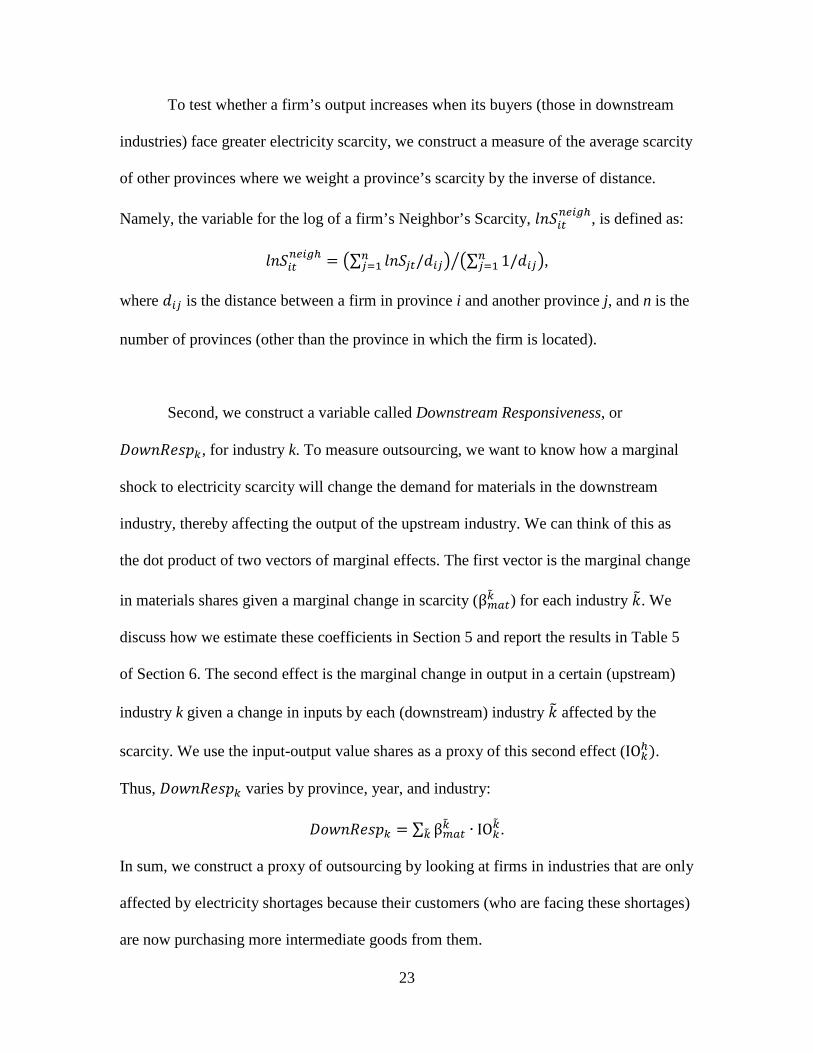
To test whether a firm’s output increases when its buyers (those in downstream

industries) face greater electricity scarcity, we construct a measure of the average scarcity

of other provinces where we weight a province’s scarcity by the inverse of distance.

Namely, the variable for the log of a firm’s Neighbor’s Scarcity, 𝑙𝑙𝑆𝑖𝑔𝑛𝑒𝑖𝑔ℎ, is defined as:

𝑙𝑙𝑆𝑖𝑔𝑛𝑒𝑖𝑔ℎ = �∑ 𝑙𝑙𝑆𝑗𝑔/𝑃𝑖𝑗𝑛

𝑗=1 � �∑ 1/𝑃𝑖𝑗𝑛𝑗=1 �� ,

where 𝑃𝑖𝑗 is the distance between a firm in province i and another province j, and n is the

number of provinces (other than the province in which the firm is located).

Second, we construct a variable called Downstream Responsiveness, or

𝐷𝑃𝐷𝑙𝐷𝑃𝐷𝐷𝑃, for industry k. To measure outsourcing, we want to know how a marginal

shock to electricity scarcity will change the demand for materials in the downstream

industry, thereby affecting the output of the upstream industry. We can think of this as

the dot product of two vectors of marginal effects. The first vector is the marginal change

in materials shares given a marginal change in scarcity (β𝑒𝑒𝑔𝑃� ) for each industry 𝑃� . We

discuss how we estimate these coefficients in Section 5 and report the results in Table 5

of Section 6. The second effect is the marginal change in output in a certain (upstream)

industry k given a change in inputs by each (downstream) industry 𝑃� affected by the

scarcity. We use the input-output value shares as a proxy of this second effect (IO𝑃ℎ).

Thus, 𝐷𝑃𝐷𝑙𝐷𝑃𝐷𝐷𝑃 varies by province, year, and industry:

𝐷𝑃𝐷𝑙𝐷𝑃𝐷𝐷𝑃 = ∑ β𝑒𝑒𝑔𝑃� ∙ IO𝑃𝑃�

𝑃� .

In sum, we construct a proxy of outsourcing by looking at firms in industries that are only

affected by electricity shortages because their customers (who are facing these shortages)

are now purchasing more intermediate goods from them.

24

5. Empirical Model

To test the four hypotheses presented in Section 3, we begin by examining the

neutral and factor-biased productivity effects of electricity shortages. From these effects,

we look for evidence of reductions of productivity (Hypothesis 1), self generation

(Hypothesis 2), outsourcing (Hypothesis 3), and energy efficiency improvements

(Hypothesis 4). We then conduct further tests of self generation and outsourcing. Our

empirical strategy is described below.

Method to Measure the Effect on Productivity

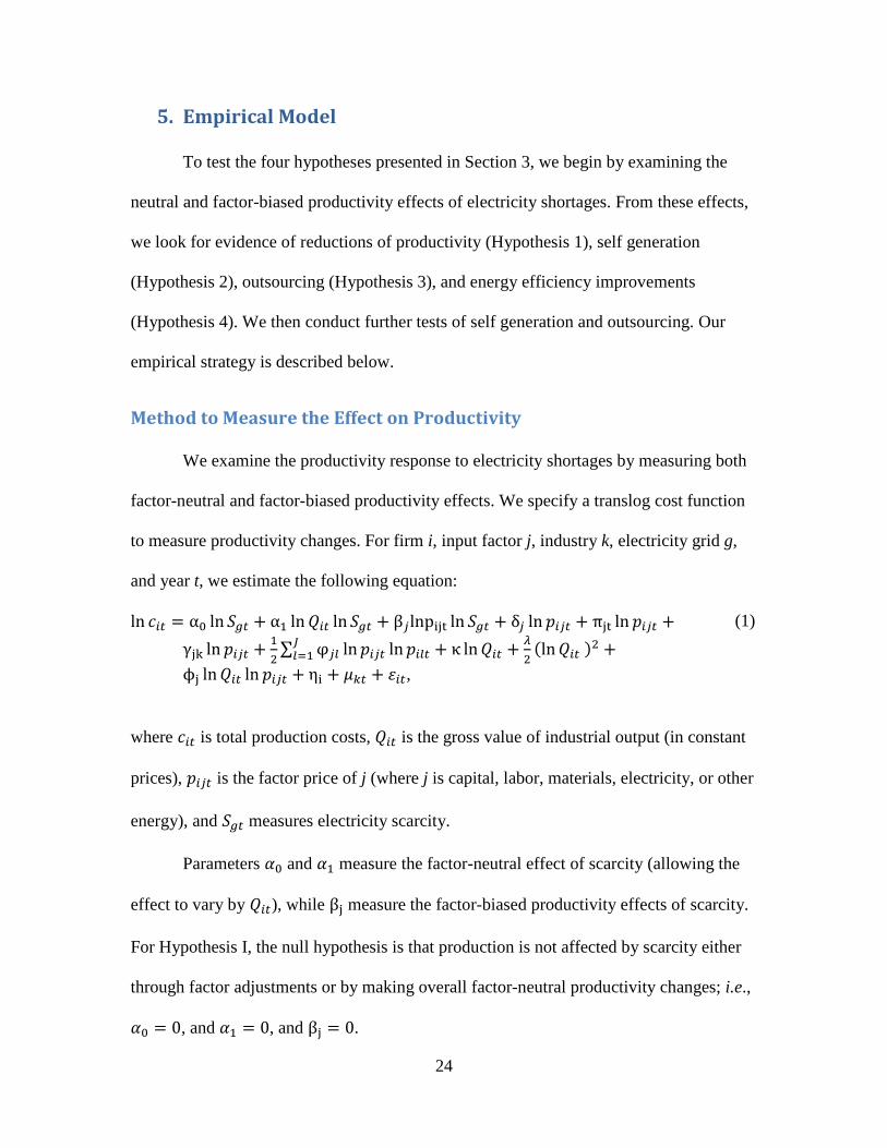
We examine the productivity response to electricity shortages by measuring both

factor-neutral and factor-biased productivity effects. We specify a translog cost function

to measure productivity changes. For firm i, input factor j, industry k, electricity grid g,

and year t, we estimate the following equation:

ln 𝑐𝑖𝑔 = α0 ln 𝑆𝑔𝑔 + α1 ln𝑄𝑖𝑔 ln 𝑆𝑔𝑔 + β𝑗lnpijt ln 𝑆𝑔𝑔 + δ𝑗 ln 𝐷𝑖𝑗𝑔 + πjt ln 𝐷𝑖𝑗𝑔 +γjk ln 𝐷𝑖𝑗𝑔 + 1

2∑ φ𝑗𝑒 ln𝐷𝑖𝑗𝑔 ln𝐷𝑖𝑒𝑔𝐽𝑒=1 + κ ln𝑄𝑖𝑔 + 𝜆

2(ln𝑄𝑖𝑔 )2 +

ϕj ln𝑄𝑖𝑔 ln 𝐷𝑖𝑗𝑔 + ηi + 𝜇𝑃𝑔 + 𝜀𝑖𝑔,

(1)

where 𝑐𝑖𝑔 is total production costs, 𝑄𝑖𝑔 is the gross value of industrial output (in constant

prices), 𝐷𝑖𝑗𝑔 is the factor price of j (where j is capital, labor, materials, electricity, or other

energy), and 𝑆𝑔𝑔 measures electricity scarcity.

Parameters 𝛼0 and 𝛼1 measure the factor-neutral effect of scarcity (allowing the

effect to vary by 𝑄𝑖𝑔), while βj measure the factor-biased productivity effects of scarcity.

For Hypothesis I, the null hypothesis is that production is not affected by scarcity either

through factor adjustments or by making overall factor-neutral productivity changes; i.e.,

𝛼0 = 0, and 𝛼1 = 0, and βj = 0.

25

For each factor input, we also estimate a factor value share equation (1) based on

Shephard’s Lemma:

𝑣𝐷ℎ𝑖𝑗𝑔 = 𝛽𝑗 ln 𝑆𝑔𝑔 + 𝛿𝑗 + 𝜋𝑗𝑔 + 𝛾𝑗𝑃 +12�φ𝑗𝑒 ln𝐷𝑖𝑒𝑔

𝐽

𝑒=1

+ ϕj ln𝑄𝑖𝑔 + 𝜉𝑖𝑔

(2)

Equations (1) and (2) represent a system of equations in which shocks to the factor shares

are likely to be correlated across the error structure of the model. As such, we estimate

equations (1) and (2) as a seemingly-unrelated regression (SUR). In order to have an

invertible disturbance covariance matrix, we drop the value share equation for materials

from the estimation.23

Furthermore, Shepard’s Lemma and ensuring that value shares sum to one (by

construction in the data) require that the coefficients exhibit the usual properties of

symmetry and homogeneity of degree one in prices. Thus, we impose the following

constraints on the model:

𝜑𝑗𝑒 = 𝜑𝑒𝑗;�𝛿𝑗 = 1𝐽

𝑗=1

;�𝛽𝑗 =𝐽

𝑗=1

�𝜑𝑗 =𝐽

𝑗=1

�𝜋𝑗 =𝐽

𝑗=1

�𝛾𝑗 =𝐽

𝑗=1

�𝜙𝑗 = 0𝐽

𝑗=1

. (3)

See Fisher-Vanden and Jefferson (2008) for further discussion of these assumptions using

these data and a similar specification.24 Note that even though some firms only appear

23 Since the factor value shares, by construction, sum to one, we can drop one of the factor value share equations – the value share equation for materials. Coefficient estimates and standard errors will be invariant to the choice of which value share equation is dropped (see Berndt, 1991). 24 We use Wald tests to estimate these assumptions (reflected in ~115 constraints in the model) in our case. We find that about half of the tests rejected the constraints. Nonetheless, we impose the symmetry restrictions on the model since the value share equations are derived from Shepard’s Lemma, and therefore symmetry between the original cost function and the value share equations must hold by construction. The h.o.d. 1 in prices restrictions ensure that value shares sum to 1, which is how value shares are defined in the data. Lastly, we adopt the translog cost function formulation as it is a flexible function that has been widely used and accepted for productivity work that tries to measure factor-biased productivity effects (see, e.g., Berndt, 1991), which is important for addressing our question of interest: how does electricity scarcity affect factor shares?

26

once in our sample, they help identify the parameters because there are no fixed effects in

the first-order equations (2) and we impose cross-equation constraints. In the analysis

below, we measure the aggregate effect of scarcity on production by estimating the

system of equations (1)-(2).25 Then we test for heterogeneous effects by separately

estimating these equations by industry.

Economists estimate productivity effects with either production or cost functions.

Both approaches may have to address concerns of endogeneity. Endogeneity concerns

exist in the estimation of production functions since some input quantities could be

simultaneously determined. Cost functions avoid this problem since input prices are used

which are assume to be exogenously determined. We, therefore, adopt the cost function

approach in our analysis which requires considering the endogeneity of output. To

address this concern, we first explore potential instruments that proxy for demand

shifters. While there are not a plethora of publicly available Chinese data sets, we were

able to measure provincial annual population and income. Unfortunately, the first stage

was weak. Therefore, instead, we use a set of firm fixed effects (𝜂𝑖) and industry-year

fixed effects (𝜇𝑃𝑔) to address the endogeneity concerns regarding output. As a robustness

check, we report a model imposing constant returns to scale, akin to making the

dependent variable average costs.

25 If we estimate only equation (1) while imposing the constraints in equation (3), then the parameter estimates become quite noisy (though the main results lie within the 95 percent confidence interval). For these estimates, we find that predicted mean value shares differ substantially from those observed in the data. This is not the case for our main approach. Furthermore, if we estimate equation (1) without any constraints (i.e., with OLS), we find negative shares for capital and materials. Note that with a large enough sample, we would expect the estimation of only equation (1) with constraints to be consistent with our findings. However, given our sample size, we follow the literature (Berndt 1991) in estimating the system implied by Shepard’s Lemma in order to improve the precision of our estimates.

27

Throughout the paper, we instrument for scarcity to address the measurement

error and endogeneity concerns mentioned in Section 4. The weather instruments separate

out CDD and HDD, as past research shows a non-monotonic relationship between

electricity consumption and temperature (for example, see Mansur, Mendelsohn, and

Morrison (2008) and Deschenes and Greenstone (2011)). Furthermore, we interact both

weather variables with all of the variables where scarcity is in equation (1). The resulting

first-stage regression is shown in equation (4):

ln 𝑆𝑔𝑔 = τ1𝐶𝐷𝐷𝑖𝑔 + τ2𝐻𝐷𝐷𝑖𝑔 + ∑ φ𝑗𝑒 ln 𝐷𝑖𝑗𝑔 ln 𝐷𝑖𝑒𝑔𝐽𝑒=1 + σ1𝑗lnpijt𝐶𝐷𝐷𝑖𝑔 +

σ2𝑗lnpijt𝐻𝐷𝐷𝑖𝑔 + δ𝑗 ln 𝐷𝑖𝑗𝑔 + πjt ln 𝐷𝑖𝑗𝑔 + γjk ln 𝐷𝑖𝑗𝑔 +12∑ φ𝑗𝑒 ln𝐷𝑖𝑗𝑔 ln 𝐷𝑖𝑒𝑔𝐽𝑒=1 + κ ln𝑄𝑖𝑔 + 𝜆

2(ln𝑄𝑖𝑔 )2 + ϕj ln𝑄𝑖𝑔 ln 𝐷𝑖𝑗𝑔 + ηi +

𝜇𝑃𝑔 + 𝜀𝑖𝑔.

(4)

We do not impose constraints on this reduced-form equation. Typically we would

incorporate this into a three-stage least squares estimation along with equations (1) and

(2) while imposing constraints (3). However, given the substantial parameter estimates

that include two full sets of firm fixed effects, this was not computationally feasible.

Thus, we chose a seemingly-unrelated regression approach using fitted values from a

first-stage instrumental variables estimation (SUR-IV) as our main specification.

In the first stage, we estimate equation (4) and predict the level of scarcity, ln �̂�𝑔𝑔.

Appendix Table A6 reports the weather coefficient estimates, including positive and

significant direct effects of both CDD and HDD on scarcity as expected. The set of

instruments are strong predictors of scarcity.26 We then replace the log of scarcity, and its

interactions with factor prices and the log of output, with our predicted ln �̂�𝑔𝑔 and the

26 F-statistic is 12.4 when we cluster the standard errors at the level we measure scarcity, by grid and year. The F-statistic is 1293 if the standard errors are assumed to be i.i.d.

28

respective interactions, in the SUR model of equations (1) and (2). This allows us to

impose the constraints of equation (3) while also addressing the concern of endogeneity.

We also examine a model where we do not instrument for scarcity. Results are discussed

below.

Our cost function estimation allows us to compute the marginal and total effects

of electricity scarcity on costs. The calculation of the marginal effect follows directly

from equation (1):

𝜕𝑐𝑖𝑔𝜕𝑆𝑔𝑔

=𝛼0𝑐𝑖𝑔 + 𝛼1 ln𝑄𝑖𝑔𝑐𝑖𝑔

𝑆𝑔𝑔+ �

𝛽𝑗 ln 𝐷𝑖𝑗𝑔𝑐𝑖𝑔𝑆𝑔𝑔

𝐽

𝑗=1

. (5)

The first term captures the factor-neutral effects while the factor-biased effects are the

remainder. Our calculations of marginal and total effects are provided below.

Method to Test for Evidence of Self Generation

Our approach to test for self generation in response to electricity shortages is two-

pronged. We first look for evidence of self generation in the productivity estimates

described above. If firms are self-generating in response to electricity scarcity, we would

expect to see a decline in the use of electricity in production, and an increase in the use of

non-electricity energy and capital—i.e., the coefficient associated with the interaction of

electricity and scarcity should be negative, the coefficient associated with the interaction

of non-electricity energy and scarcity should be positive, and the coefficient associated

with the interaction of capital and scarcity should be positive.

We test the self-generation hypothesis further by estimating separate regressions

on self-generation indicators using an instrumental variables approach. The dependent

variable is either the share of energy consumption that is used to generate electricity, or

29

the indicator variable of self generation. For the latter, we assume a linear probability

model of adoption decisions. We use the same weather variables as above. Firm and

industry-year fixed effects are included in estimating (6):27

𝑆𝑃𝑙𝑆𝑖𝑔 = ψ𝑃𝑙𝑙𝑆𝑔𝑔 + ηi + 𝜇𝑃𝑔 + 𝜀𝑖𝑔 (6)

We cluster the standard errors by firm to control for serial correlation.

For each industry, we test whether a firm’s decision to self generate depends on

the electricity grid’s scarcity measure. It is reasonable to believe that firms using a

substantial amount of power are more likely to self generate when faced with electricity

shortages. As our sample is of the largest energy users in China, we likely capture most

of the firms that would fit this criterion. However, energy consumption is not necessarily

the driving factor in a firm’s decision to self generate. It could also be the case that firms

would self generate if they would suffer the most from a shutdown. This includes firms in

industries that need to finish a process without interruption: a blackout would mean

restarting the process anew. Rather than label industries as continuous or batch producers,

we estimate the effects for each industry separately. Lastly, it is important to note that the

decision to self generate may differ substantially in the long run. We are only able to

measure how firms responded to contemporaneous electricity shortages.

Method to Test for Evidence of Outsourcing

Similar to self generation, we take a two-pronged approach to test for outsourcing

in response to electricity scarcity. We first look for evidence for outsourcing in the factor-

27 Given that some firms show up only once and that this is a linear model with firm fixed effects, we drop over 16,000 observations from the single-year firms.

30

biased productivity estimations. Outsourcing is consistent with a simultaneous reduction

in the use of electricity and an increase in the purchase of materials inputs to productions.

We can also test for outsourcing on the supply side. That is, if a firm decides to

outsource intermediate inputs, we should see an increase in the production of potential

suppliers to this firm. To test for this, we measure how firms located in a (particularly

nearby) province that is not facing scarcities are affected by electricity scarcities in other

provinces. If a firm is located in an electricity grid that is not suffering electricity

shortages, but is located near a newly affected province, then we would expect to see the

firm increase production. This is especially true for firms that are suppliers to firms in

industries that are most affected by electricity shortages.

We regress the natural logarithm of gross value of industrial output in constant

prices of firm i in year t, or output (𝑄𝑖𝑔), on the log of scarcity that firm i faces in grid g

(𝑙𝑙𝑆𝑔𝑔), the log of its neighbor’s scarcity (𝑙𝑙𝑆𝑖𝑔𝑛𝑒𝑖𝑔ℎ), as defined in Section 4, and the

interaction between the neighbor’s scarcity and our measure of downstream

responsiveness of firm i in industry k (𝐷𝑃𝐷𝑙𝐷𝑃𝐷𝐷𝑃), also defined in Section 4. Similar to

the self-generation regressions, we instrument for scarcity using weather data, include

firm fixed effects and industry-year fixed effects, exclude firms that only report once, and

cluster the standard errors by firm in estimating equation (7):

ln(𝑄𝑖𝑔) = 𝜃1𝑙𝑙𝑆𝑔𝑔 + 𝜃2𝑙𝑙𝑆𝑖𝑔𝑛𝑒𝑖𝑔ℎ + 𝜃3𝑙𝑙𝑆𝑖𝑔

𝑛𝑒𝑖𝑔ℎ ∗ 𝐷𝑃𝐷𝑙𝐷𝑃𝐷𝐷𝑃 + ηi + 𝜇𝑃𝑔 + 𝜀𝑖𝑔 (7)

31

6. Results

Table 4 reports the main results from estimating the system of equations (1) and

(2). The first column (SUR-IV) reports our main specification.28 Our results suggest that

scarcity—defined as the ratio of generation to capacity, which captures the potential for

or threat of shortages—affects how firms produce. Namely, scarcity leads to significant

substitutions among the five factor inputs. Increased scarcity leads to a reduction in the

use of electricity and other forms of energy and an increase in the use of materials. These

results suggest that a 10% increase in scarcity will increase the cost share of materials by

about two percent and will decrease the cost shares of electricity and other energy by

about half that amount. The effects on labor and capital are even smaller.

This effect on materials suggests that, when electricity becomes scarce, firms will

outsource the production of intermediate inputs (rather than to produce these inputs in-

house), which is consistent with our third hypothesis. We do not, however, find evidence

to support our hypothesis that electricity shortages will lead to greater self generation. We

observe neither an increase in capital use, nor a substitution toward other types of energy

(in particular diesel oil) that would be consistent with self generation. To the contrary, we

see a significant reduction in non-electric energy. At first, this effect on energy overall

seems consistent with the hypothesis that electricity shortages lead to energy efficiency

improvements. However, we do not see an increase in capital. Hence, outsourcing

appears the only hypothesis for which we find evidence in our productivity estimates.

The overall effect on unit costs is a combination of both the factor-biased and

factor-neutral effects. We explore this net effect in the following section. Table 4,

28 Appendix Table A7 provides coefficient estimates for all variables excluding the firm fixed effects.

32

however, reports a negative factor-neutral effect of scarcity—i.e., an increase in scarcity

lowers the total cost of production—which suggests that, holding inputs constant, firms

may have been pushed to improve overall productivity during times of scarcity. However

this effect is not statistically significant. Furthermore, the effect dissipates with firm size

(Qit) due to the positive coefficient on the interaction of scarcity and GVIO: for the

smallest firms (at 1st percentile), the factor-neutral effect is -0.35 while the largest firms

(at the 99th percentile) the effect is only -0.01. Both are insignificant.

The second column of Table 4 treats scarcity as exogenous by using the direct

measure of scarcity and not its predicted value based on our IV regression. The

coefficients are extremely similar to the main results. Nonetheless, throughout the rest of

the paper, we continue with the instrumental variables approach given our concerns of

measurement error and omitted variables bias previously discussed.

Columns 3 and 4 restrict the main SUR-IV specification. The third column

imposes a constant factor neutral scarcity effect for firms of all sizes: i.e., α1 = 0 in

equation (1). That is, we assume that the scarcity effect is not dependent on firm size by

omitting the interaction of scarcity and GVIO from the regression. Finally, the last

column assumes constant returns to scale by imposing the constraints α1 = 0, 𝜆 = 0 and

κ = 1 in equation (1). This is akin to modeling average costs as a function of scarcity. As

shown in Columns 3 and 4, imposing these restrictions does little to change the results of

our main SUR-IV specification.

Industry Heterogeneity

Table 5 reports the results when we estimate the system of equations (1) and (2)

separately for each industry. We find large responses to scarcity in electricity shares—

33

reflected in the coefficient associated with the interaction of scarcity and electricity—for

textiles, wood products, mining, and metal industries.29 Outsourcing in response to

scarcity (as suggested by a positive coefficient on the interaction of scarcity and

materials) is large in several sectors: wood products, chemicals, food, metal, and textiles.

These results also show large decreases in other energy shares for wood products,

mining, chemicals, and non-metals. The one industry that reported using more energy in

response to scarcity was petroleum, which may have greater access to energy resources.

Capital shares in response to scarcity fell in food and rubber, but rose substantially in

mining and other industries. Labor shares in response to scarcity fell in textiles and metal.

Revisiting the four hypotheses from Section 3, we find evidence of outsourcing in

most industries, with the exception of mining, petroleum, rubber, and other industries.

None of the industries produce results consistent with self generation. Positive factor-

neutral effects in the Petroleum industry—reflected in the coefficient associated with

scarcity alone—imply that electricity shortages are costly for petroleum firms, and

particularly costly for small petroleum firms (reflected in the negative coefficient

associated with the interaction of scarcity and GVIO). In contrast, in the Rubber industry,

the negative factor-neutral effect on scarcity suggests cost savings. Finally, the results in

the mining industry are consistent with improved efficiency, as the coefficients associated

with scarcity interacted with electricity and other energy are both negative and

significant. Thus, from the first-order conditions this implies that a change in scarcity

results in a decline in both the value share of electricity and other energy used in

29 These industries are composite industries comprising a number of sub-industries. For instance, Wood Products include paper, pulp, and furniture manufacturing.

34

production. Note that these differential effects across industries may be due to differences

in regulatory treatment.

Robustness

We perform several robustness checks and report the findings in the appendix. As

discuss in the Data section, our main specification is estimated on an unbalanced sample

of firms—that is, not all firms report in every year. As a robustness check, we estimate

our main specification on a balanced sample. Table A1 shows how sensitive the results

are to using a balanced panel. As previously discussed, requiring that a firm report in all

years vastly reduces the sample size. The second column of results shows estimate from

estimating our main specification on a balanced sample of firms that report in all years

between 1999-2004. We see in Column 2 that the results are qualitatively similar to our

main results (replicated in Column 1). Namely, firms shift from labor and energy (both

electricity and other energy) to materials. In this sample, we see some evidence of a

capital-intensive factor bias from scarcity. The last two columns reduce the sample to just

the balanced sample starting in 2000 and 2001, respectively. With fewer years, more

firms are in these balanced samples. We see similar results with the sample starting in

2000 as with the sample starting in 1999.

In Column 2 of Table A2 we drop all 2004 observations. We find that the effects

of electricity scarcity on factor shares are similar to our main results. As an additional

test, we estimate the model on subsamples that exclude observations from 2004 that

would be considered outliers, based on energy use in the 2003 sample. Specifically, we

first truncate the sample by omitting 2004 observations where the total energy use (in

heat content) in that year is below the 2003 sample minimum (resulting in 336

35

observations being dropped). We create a second subsample by dropping observations in

2004 that were below the first percentile of the 2003 sample distribution (resulting in

5288 observations being dropped). As shown in columns 3 and 4 of Table A2, we find

that the estimates of the effect of scarcity on factor shares are nearly identical to our main

results when we estimate the model on both subsamples. We conclude that the main

results seem robust to alternative samples where 2004 observations were omitted.

Table A4 presents results from several robustness checks on alternative sub-

samples of the data. Column 1 reports the results for the State-Owned Enterprises (SOE)

only. Column 2 reports the results for non-state-owned firms. We find qualitatively

similar results with both samples, with the SOE results somewhat smaller in magnitude.

For example, the coefficient on materials is 0.191 in our main specification, 0.069 for

SOEs, and 0.215 for other firms. The main difference is that the SOE results show a

significant capital-using effect of scarcity while the non-SOE results show a significant

capital-saving effect of scarcity. This averages out to an insignificant capital-saving effect

in the main results.

Columns 3 and 4 of Table A4 examine regional variation. While it would be

interesting to test if the main results are similar in each electricity grid, we cannot directly

test this given our measure of scarcity and our specification. Namely, our scarcity

measure varies over grid and year only. In addition, we include industry-year fixed

effects in our analysis in order to control for unobserved trends that would be hard to

justify excluding. In Column 3, we drop the region with the greatest variation, the North,

and test whether there remains sufficient variation in the other regions. In the table, we

see results similar to our main findings. Column 4 drops the East, which is the largest

36

region. For a given level of electricity scarcity, we may believe that small regions will

have a harder time responding to threats of blackouts by smoothing the scarcity over

customers. When we drop the largest region, however, we do not see an increase in the

parameter estimates among the smaller regions.

Table A5 tests whether our results are robust to the two alternative measures of

scarcity discussed in Section 4, peak load and all capacity. The results are qualitatively

similar to our main specification. However, the preferred scarcity measure shows the

greatest response. This suggests that the peak measure does not capture all of the

response to electricity shortages and that the measure including hydropower capacity

(“all capacity”) may exhibit measurement error, as discussed in Section 4.

Finally, Column 4 of Table A5 shows results for a placebo test. Recall that our

energy data consists of two samples. From 1999 to 2003, we have data on just the most

energy intensive firms in China. Not surprisingly, this is an unlikely group to be

unaffected by electricity shortages. In Table 5, we saw that every industry changed their

factor shares in some way: Even the industries that are less energy intensive, like the food

and machinery industries, increased materials shares and reduced shares of electricity and

of other energy. The second sample for our energy data comes from the 2004 census

which includes all large and medium firms, not just the most energy intensive. We exploit

this difference in sampling to construct a group of firms that are not very energy

intensive: namely, the firms that show up in the 2004 only. As we have financial data on

these firms, they are still medium to large in size making them a reasonable control

group. The downside is that we only observe these firms once and therefore need to adopt

a cross sectional approach to our estimation. We drop the firm fixed effects and include

37

time-invariant controls including indicators of industry and ownership. The table shows

that none of the factor bias effects of scarcity are significantly different from zero.

Therefore, we do not find evidence of outsourcing in response to electricity scarcity

among firms that are less energy-intensive. Since only the most energy-intensive firms

experience a drop in the use of electricity and an increase in the purchases of materials,

this bolsters our belief that firms that are most exposed to electricity shortages are

responding by outsourcing.

Self Generation

Table 6 reports the estimates of equation (6) on self generation by industry. The

first panel examines the indicator variable of self generation. The coefficients are large

for many industries, but the estimates are noisy. For example, mining and food both have

positive coefficients suggesting greater self generation during greater times of scarcity,

but the estimates are insignificant at the 10% level. We do find significant, but negative,

effects for wood products, chemical, metal, and other industries. These findings are

consistent with our cost function results, which do not support the hypothesis that firms

chose to self generate in reaction to electricity shortages (Hypothesis II in Section 3).

Table 6 also includes the mean of the dependent variable. We see that self generation is

most common in mining, food, and petroleum. Even in these industries, less than 20% of

firms self generate.

Panel B of Table 6 reports the results when the dependent variable is the share of

energy consumption used to generate electricity. Again, the estimates are noisy. The

largest positive effects are in non-metal and mining but are insignificant. In these

regressions, we find negative coefficients on the self-generation rate, which are

38

statistically significant at the 5% level, for chemicals and metal industries, suggesting that

scarcity leads to less self generation in these industries. We report the mean of the

dependent variable and see that no industry uses more than eight percent of its total

energy consumption to generate electricity.

We conclude that the firms in our sample do not self generate electricity often,

and, even those with the capability, do not depend on self generation to supply power.

We find no evidence consistent with firms investing in generators to address electricity

shortages.

Appendix Table A8 provides robustness tests of the results, pooling across all

industries (i.e. for the average firm across industries), using alternative models. Columns

1 and 3 estimate the effects for our two measures of self generation (the indicator and

share variables, respectively) using the model used in Table 6—i.e., a linear model with

firm fixed effects—but pooled across industries. In Column 2, we drop the firm fixed

effects and estimate a random effects probit model where we include time-invariant

indicator variables for region, industry, and ownership. In Column 4, we estimate a

random effects Tobit model with similar controls. In all specifications, we find no

evidence of self generation.

Note that these effects are identified off of just a few years of data,

contemporaneous with the height of the power shortages. Installing new capital-intensive

equipment might require more time to install. Similarly, firms may have been waiting to

determine whether or not these electricity shortages would become persistent: there was

option value in waiting. Finally, while there were reports of firms and residents installing

self generation (Rosen and Houser 2007, IEA 2006), our sample focuses on just the

39

largest energy users. For these firms, the costs of self supplying may have been extremely

large. These are reasonable explanations for the lack of evidence of self generation in our

results.

Outsourcing

As a further test of outsourcing, we estimate whether a firm’s production

increases when firms it supplies to are facing electricity shortages (namely, equation (7)).

The results are provided in Table 7. In Column 1, we include only the firm’s own scarcity

and its neighbor’s scarcity. We find evidence that firms increase output when either the

log of their own scarcity decreases or the log of their neighbor’s scarcity increases. A one

standard deviation increase in own scarcity leads to a 11% decrease in output, while a one

standard deviation increase in the neighbor’s scarcity leads to a 21% increase in output.30

Column 2 of Table 7 shows the effect of own scarcity and the interaction term

between neighbor’s scarcity and downstream responsiveness. In effect, this increases the

weight of those observations that are most likely to experience outsourcing, as their

buyers are in industries that had the largest change in materials shares in response to

increased electricity scarcity. Here we see the effect of own scarcity is less than half the

magnitude of the coefficient in Column 1, though still significant. However, the

interaction term of downstream responsiveness and neighbor’s scarcity is large and

significant. A one standard deviation increase in this variable leads to a 26% increase in

output.

30 For brevity, we stop referring to the log specification, hereafter. The standard deviations of the three variables are 0.104 for own scarcity, 0.079 for the neighbor’s scarcity, and 0.028 for the interaction term.

40

Finally, in Column 3 of Table 7, we include all three variables. Note that we do

not also include the downstream responsiveness variable as it is perfectly correlated with

the firm fixed effects. This specification tests for a differential impact in the response to

neighbor’s scarcity. We find results consistent with Column 1 for the own scarcity and

neighbor’s scarcity, and a coefficient consistent with Column 2 for the interaction term.

Namely, a one standard deviation in own scarcity, neighbor’s scarcity, and neighbor’s

scarcity interacted with downstream responsiveness result in a -11%, 17% and 23%

change in a firm’s output, respectively. However, only the coefficients on own scarcity

and the interaction of neighbor’s scarcity with downstream responsiveness are significant

(at the 10% level). These results lend further evidence that scarcity leads firms to

outsource.

7. The Costs of Shortages

How did electricity shortages during 2000-2004 affect total production costs?

Table 8 provides estimates of the change in aggregate production costs—in both Yuan

and approximate US$—holding output fixed, as a result of changes in scarcity from 1999

onward. To calculate this, we first compute the marginal cost of scarcity using equation

(5) with estimated coefficients from Table 5 and sample means for the independent

variables. We report these marginal effects in Column 1 of Panel A. Overall, the marginal

cost is 391 million Yuan. We then disaggregate this into the factor bias effect (first term

of equation (5)) and the factor neutral effect (second term of equation (5)), which are 510

and -118 million Yuan, respectively. These results imply that while shifting factor input

shares in response to a marginal increase in electricity scarcity lowers cost, loses in

41

overall productivity from a marginal increase in scarcity offset these gains. We further

disaggregate the factor bias effect for each of the five factors. We find that the shift to

materials in response to a marginal change in scarcity increases costs by 667 million

Yuan, with shifts away from labor, electricity and other energy partially offsetting this

cost increase.

Next we calculate the change in total production costs that we attribute to the

actual change in scarcity. In other words, had China continued to build power plants

allowing electricity supply to grow at the same rate as the quantity demanded grew from

1999 to 2004, how much would firms had saved in unit production costs? To estimate

this, we multiply the marginal cost of scarcity by the actual change in scarcity from 1999

to each subsequent year, and aggregate over all observations in our sample. As shown in

Column 2 of Table 8, Panel A, we find that total costs increased by 1192 billion Yuan, or

7.8% of the total realized aggregate costs of these firms from 2000 to 2004. Factor biased

effects account for this increase, with total costs increasing by 1552 billion Yuan (10.1%

of aggregate costs) due to these factor biased effects. In particular, the shift to materials

increased total production costs by 2032 billion Yuan (13.2% of aggregate costs).

Panel B of Table 8 repeats these calculations using the marginal effects calculated

separately for each observation. That is, equation (5) is evaluated using estimated

coefficients from Table 5 and observational data for the variables. Panel B reports the

mean of these calculated marginal effects by observation. Given that equation (5) is not

linear in variables, some differences from Panel A are expected. Nonetheless, the first

column of this table reports that the means of the marginal effects are similar to those in

Panel A. From 2000 to 2004, total costs increased by 1316 billion Yuan (8.6% of all

42

costs). As in the top panel, most of this is attributed to materials expenses: 1918 billion

Yuan (12.5% of all costs).

We can use the results from Table 8 to calculate the benefits, due to fewer

productivity losses, of reducing electricity scarcity. From Panel A, the marginal benefit of

reducing scarcity is 391 million Yuan for the average firm in our sample. From 2000 to

2004, Chinese electricity grids had, on average, 44 GW of fossil capacity. Suppose that a

one MW power plant were built and operated with a 50 percent capacity factor

(generating, on average, 0.5 MWh per hour). For the average grid, this would reduce

scarcity by about 1/88,000. Our sample has 1,026 firms reporting in each grid and year,

on average. Aggregating over these firms, we calculate that building an additional MW of

capacity would reduce productivity losses by about 4.6 million Yuan per year, or

USD$103 per MWh. Note that these are short run costs that were unexpected. Had firms

known of these risks, they may have invested in more self generation.31 In contrast, the

International Energy Agency (2010) estimates that a new one MW Chinese coal plant

would cost 3.8 million Yuan to build, with levelized costs of $33 per MWh. On the

margin, the productivity benefits exceed the private costs of building a new power plant.

8. Conclusion

This paper examines how firms in China responded to power shortages during the

early 2000s. We find that firms in regions with greater shortages decreased factor shares

of electricity and increased shares of materials. We do not find evidence of an increase of

31 Distributed generation levelized costs range from $90 to $220/MWh: see http://www.eia.gov/oiaf/archive/aeo09/pdf/0383(2009).pdf and http://srren.ipcc-wg3.de/report/, respectively.

43

self generation of electricity. In fact, we find an overall decrease in other non-electricity

energy sources, suggesting that these primary energy sources are complementary inputs

in producing the intermediate products that have been outsourced in response to

electricity shortages. The overall effect of electricity shortages, which we proxy for with

a measure of scarcity, was to increase production costs. From 1999 to 2004, firms’ costs

rose by eight percent, primarily due to input factor substitutions.

Policy recommendations in light of these results are difficult to determine and are

beyond the scope of this paper. Although our results would seem to suggest that more

power plants should have been built, this conclusion could only be made by trading off

the social cost of building new power plants with the benefits (e.g., the avoidance of

productivity losses from electricity scarcity). As discussed in Section 7, we calculate that

a one MW power plant could result in benefits in improved productivity each year that

are over 400 times greater than the levelized construction costs.

Policy makers would also want to consider other mechanisms to provide reliable

service. For example, dynamic pricing that reflects electricity firms’ actual marginal costs

would be an option. While we do not address these questions, our results help determine

how costly the electricity shortages were in China between 1999 and 2004.

44

References

Abeberese, Ama Baafra. 2014. “The Effect of Electricity Shortages on Firm Investment: Evidence from Ghana,” Manuscript, Wellesley College.

Alby, Philippe, Jean-Jacques Detherier, and Sèphane Straub. 2011. “Let There be Light! Firms Operating under Electricity Constraints in Developing Countries,” Toulouse School of Economics Working Paper 11-255.

Allcott, Hunt, Allan Collard-Wexler, and Stephen D. O’Connell. 2014. “How Do Electricity Shortages Affect Productivity? Evidence from India,” Manuscript, New York University.

Baisa, Brian, Lucas Davis, Stephen Salant, and William Wilcox. 2010. “The Welfare Costs of Unreliable Water Service,” Journal of Development Economics, 92(1), 1-12.

Berndt, Ernst R. 1991. The Practice of Econometrics: Classic and Contemporary. Addison-Wesley Publishing Co.

Borenstein, Severin and Joseph Farrell. 2007. “Do Investors Forecast Fat Firms? Evidence from the Gold Mining Industry,” Rand Journal of Economics, 38(3): 626-647.

Chen, Lijuan, and Lixiong Jia. 2006. “Reliability of Nationwide Transmission and Substation Facilities and Urban Consumer’s Power Supply in 2005,” Electricity, 3: 45-51.

de Kok, A.G. and S.C. Graves, eds. 2003. Handbook in Operations Research and Management Science: Supply Chain Management: Design, Coordination and Operation, Volume 11, Elsevier, Amsterdam.

Deschenes, Olivier and Michael Greenstone. 2011. “Climate Change, Mortality, and Adaptation: Evidence from Annual Fluctuations in Weather in the US,” American Economic Journal: Applied Economics, 3(4): 152-185.

Dick, Andrew. 1992. “An Efficiency Explanation for Why Firms Second Source,” Economic Inquiry, 30(2): 332-354.

Dong, Baomin and Xuefeng Li. Forthcoming. “Estimating Outage Costs in China: A Modified Tobit Model,” Emerging Markets Finance and Trade.

Energy Information Administration (EIA). 2009. International Energy Outlook, 2009. U.S. Department of Energy, Washington, DC.

Engle, Robert F., C. W. J. Granger, John Rice, and Andrew Weiss. 1986. “Semiparametric Estimates of the Relation between Weather and Electricity Sales,” Journal of the American Statistical Association, 81(394): 310-320.

Fisher-Vanden, Karen. 2009. “Energy in China: Past Trends and Future Directions,” International Review of Environmental and Resource Economics, 3(3): 217-244.

Fisher-Vanden, Karen, and Gary Jefferson. 2008. “Technology Diversity and Development: Evidence from China’s Industrial Enterprises,” Journal of Comparative Economics, 36(4): 658-672.

International Energy Agency (IEA). 2006. “China’s Power Sector Reforms: Where to Next?” Paris: OECD.

IEA. 2007. “World Energy Outlook, 2007: China and India Insights,” Paris: OECD. IEA. 2010. “Projected Costs of Generating Electricity,” OECD/IEA, Paris,

http://www.iea.org/publications/freepublications/publication/projected_costs.pdf.

45

Jyoti, Roop, Aygul Ozbafli, and Glenn Jenkins. 2006. “The Opportunity Cost of Electricity Outages and Privatization of Substations in Nepal,” Queen’s University, Department of Economics, Working Paper \#1066, 24 pp.

Lee, Chien-Chiang, and Yi-Bin Chiu. 2011. “Electricity Demand Elasticities and Temperature: Evidence from Panel Smooth Transition Regression with Instrumental Variable Approach,” Energy Economics, 33(5): 896-902.

Lin, B., B. Dong, and X. Li. 2005. “An Econometric Analysis on the Power Shortages and Outages.” Manuscript, Department of Economics, University of International Business and Economics, Beijing, China.

Mansur, Erin T., Robert Mendelsohn, and Wendy Morrison. 2008. “Climate Change Adaptation: A Study of Fuel Choice and Consumption in the US Energy Sector,” Journal of Environmental Economics and Management}, 55(2): 175-193.

Natural Resources Defense Council. 2003. “Demand Side Management in China: Benefits, Barriers, and Policy Recommendations.” www.nrdc.org/air/energy/chinadocs/dsm.pdf. Accessed April 02, 2007.

National Bureau of Statistics (NBS). 2007. “China Statistical Yearbook, 2007,” Beijing, PR China.

Pao, H.-T. 2006. “Comparing Linear and Nonlinear Forecasts for Taiwan’s Electricity Consumption,” Energy 31, 2129–2141.

Reinikka, Ritva and Jakob Svensson. 2002. “Coping with Poor Public Capital,” Journal of Development Economics, 69: 51-69.

Rosen, D.H., and T. Houser. 2007. “China Energy: A Guide for the Perplexed,” Peterson Institute for International Economics, Washington, DC.

Thompson, E. 2005. “Power Shortages in China: Why?” China: An International Journal, 3(1): 155 -- 171. http://muse.jhu.edu/journals/china/v003/3.1thomson.pdf. Accessed on April 13, 2007.

Wang, Juliana Qiong. 2007. “Background Paper: The Power Sectors in China -- Development, Reform, and Shortages.” Manuscript, Yale University.

Wooldridge, Jeffrey M. 2006. Introductory Econometrics: A Modern Approach, third edition. Cincinnati, OH: South-Western

College Publishing. World Bank. 2005. “Demand-Side Management in China’s Restructured Power Industry:

How Regulation and Policy Can Deliver Demand-Side Management Benefits to a Growing Economy and a Changing Power System.” Energy Sector Management Assistance Program.

Yildirim, Kemal, Cuneyt Koyuncu, and Julide Koyuncu. 2009. “Does Temperature Affect Labor Productivity: Cross-Country Evidence,” Applied Econometrics and International Development 9.1: 29-38.

Zhou, Shaojie, and Fei Teng. 2013. “Estimation of Urban Residential Electricity Demand in China using Household Survey Data,” Energy Policy 61: 394–402.

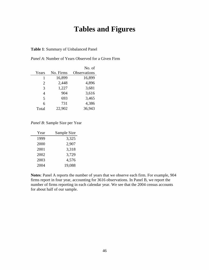
46

Tables and Figures

Table 1: Summary of Unbalanced Panel

Panel A: Number of Years Observed for a Given Firm

Years No. Firms No. of

Observations 1 16,899 16,899 2 2,448 4,896 3 1,227 3,681 4 904 3,616 5 693 3,465 6 731 4,386

Total 22,902 36,943

Panel B: Sample Size per Year

Year Sample Size 1999 3,325 2000 2,907 2001 3,318 2002 3,729 2003 4,576 2004 19,088

Notes: Panel A reports the number of years that we observe each firm. For example, 904 firms report in four year, accounting for 3616 observations. In Panel B, we report the number of firms reporting in each calendar year. We see that the 2004 census accounts for about half of our sample.

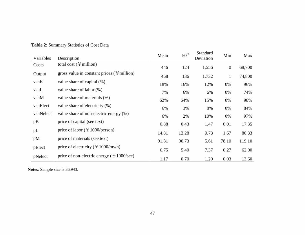
47

Table 2: Summary Statistics of Cost Data

Variables Description Mean 50th Standard Deviation Min Max

Costs total cost (￥million) 446 124 1,556 0 68,700

Output gross value in constant prices (￥million) 468 136 1,732 1 74,800

vshK value share of capital (%) 18% 16% 12% 0% 96% vshL value share of labor (%) 7% 6% 6% 0% 74% vshM value share of materials (%) 62% 64% 15% 0% 98% vshElect value share of electricity (%) 6% 3% 8% 0% 84% vshNelect value share of non-electric energy (%) 6% 2% 10% 0% 97% pK price of capital (see text) 0.88 0.43 1.47 0.01 17.35 pL price of labor (￥1000/person)

14.81 12.28 9.73 1.67 80.33 pM price of materials (see text) 91.81 90.73 5.61 78.10 119.10 pElect price of electricity (￥1000/mwh)

6.75 5.40 7.37 0.27 62.00 pNelect price of non-electric energy (￥1000/sce)

1.17 0.70 1.20 0.03 13.60 Notes: Sample size is 36,943.

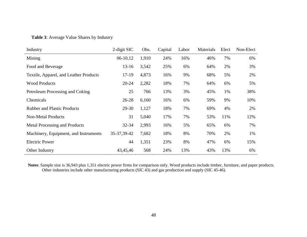
48

Table 3: Average Value Shares by Industry

Industry 2-digit SIC Obs. Capital Labor Materials Elect Non-Elect

Mining 06-10,12 1,910 24% 16% 46% 7% 6%

Food and Beverage 13-16 3,542 25% 6% 64% 2% 3%

Textile, Apparel, and Leather Products 17-19 4,873 16% 9% 68% 5% 2%

Wood Products 20-24 2,282 18% 7% 64% 6% 5%

Petroleum Processing and Coking 25 766 13% 3% 45% 1% 38%

Chemicals 26-28 6,160 16% 6% 59% 9% 10%

Rubber and Plastic Products 29-30 1,127 18% 7% 69% 4% 2%

Non-Metal Products 31 5,040 17% 7% 53% 11% 12%

Metal Processing and Products 32-34 2,993 16% 5% 65% 6% 7%

Machinery, Equipment, and Instruments 35-37,39-42 7,682 18% 8% 70% 2% 1%

Electric Power 44 1,351 23% 8% 47% 6% 15%

Other Industry 43,45,46 568 24% 13% 43% 13% 6%

Notes: Sample size is 36,943 plus 1,351 electric power firms for comparison only. Wood products include timber, furniture, and paper products. Other industries include other manufacturing products (SIC 43) and gas production and supply (SIC 45-46).

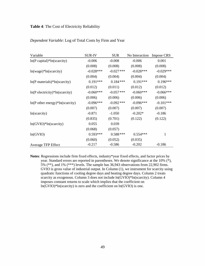
49

Table 4: The Cost of Electricity Reliability

Dependent Variable: Log of Total Costs by Firm and Year

Variable SUR-IV SUR No Interaction Impose CRS ln(P capital)*ln(scarcity) -0.006 -0.008 -0.006 0.001 (0.008) (0.008) (0.008) (0.008) ln(wage)*ln(scarcity) -0.028 *** -0.027 *** -0.028 *** -0.029 *** (0.004) (0.004) (0.004) (0.004) ln(P materials)*ln(scarcity) 0.191 *** 0.184 *** 0.191 *** 0.196 *** (0.012) (0.011) (0.012) (0.012) ln(P electricity)*ln(scarcity) -0.060 *** -0.057 *** -0.060 *** -0.066 *** (0.006) (0.006) (0.006) (0.006) ln(P other energy)*ln(scarcity) -0.096 *** -0.092 *** -0.096 *** -0.101 *** (0.007) (0.007) (0.007) (0.007) ln(scarcity) -0.871 -1.050 -0.202 * -0.186 (0.835) (0.701) (0.122) (0.122) ln(GVIO)*ln(scarcity) 0.055 0.039 (0.068) (0.057) ln(GVIO) 0.593 *** 0.588 *** 0.554 *** 1 (0.060) (0.052) (0.035) Average TFP Effect -0.217 -0.586 -0.202 -0.186 Notes: Regressions include firm fixed effects, industry*year fixed effects, and factor prices by

year. Standard errors are reported in parentheses. We denote significance at the 10% (*), 5% (**), and 1% (***) levels. The sample has 36,943 observations from 22,902 firms. GVIO is gross value of industrial output. In Column (1), we instrument for scarcity using quadratic functions of cooling degree days and heating degree days. Column 2 treats scarcity as exogenous. Column 3 does not include ln(GVIO)*ln(scarcity). Column 4 imposes constant returns to scale which implies that the coefficient on ln(GVIO)*ln(scarcity) is zero and the coefficient on ln(GVIO) is one.

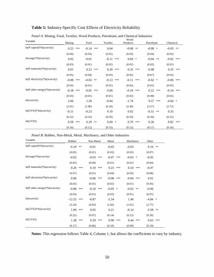
50

Table 5: Industry-Specific Cost Effects of Electricity Reliability Panel A: Mining, Food, Textiles, Wood Products, Petroleum, and Chemical Industries

Variable Mining Food Textiles Wood

Products Petroleum Chemical

ln(P capital)*ln(scarcity) 0.23 *** -0.14 *** 0.04

-0.08 ** -0.08 * -0.03 **

(0.04)

(0.03)

(0.02)

(0.03)

(0.04)

(0.02) ln(wage)*ln(scarcity) 0.02

-0.01

-0.11 *** 0.04 * -0.04 ** -0.02 ***

(0.03)

(0.01)

(0.02)

(0.02)

(0.02)

(0.01) ln(P materials)*ln(scarcity) 0.01

0.23 *** 0.20 *** 0.35 *** -0.08

0.25 ***

(0.05)

(0.04)

(0.03)

(0.05)

(0.07)

(0.03) ln(P electricity)*ln(scarcity) -0.08 *** -0.02 ** -0.13 *** -0.11 *** -0.02 * -0.06 ***

(0.02)

(0.01)

(0.01)

(0.02)

(0.01)

(0.02) ln(P other energy)*ln(scarcity) -0.18 *** -0.05 *** 0.00

-0.19 *** 0.22 *** -0.14 ***

(0.03)

(0.01)

(0.01)

(0.02)

(0.08)

(0.02) ln(scarcity) 2.66

1.29

-0.94

-1.74

9.57 *** -4.64 *

(2.61)

(1.96)

(6.18)

(2.40)

(3.27)

(2.72) ln(GVIO)*ln(scarcity) -0.11

-0.23

0.10

0.02

-0.51 ** 0.35

(0.22)

(0.16)

(0.50)

(0.20)

(0.26)

(0.22)

ln(GVIO) 0.58 *** 0.29 ** 0.69 * 0.70 *** 0.26

0.82 ***

(0.16)

(0.12)

(0.35)

(0.15)

(0.17)

(0.16)

Panel B: Rubber, Non-Metal, Metal, Machinery, and Other Industries

Variable Rubber Non-Metal Metal Machinery Other

ln(P capital)*ln(scarcity) -0.10 ** -0.01

-0.03

-0.03

0.16 **

(0.05)

(0.01)

(0.03)

(0.02)

(0.07) ln(wage)*ln(scarcity) -0.02

-0.03 *** -0.07 *** -0.02 * -0.05

(0.03)

(0.00)

(0.01)

(0.01)

(0.04)

ln(P materials)*ln(scarcity) 0.20 *** 0.19 *** 0.23 *** 0.10 *** -0.07

(0.07)

(0.01)

(0.04)

(0.03)

(0.08) ln(P electricity)*ln(scarcity) 0.00

-0.06 *** -0.08 *** -0.04 *** 0.01

(0.03)

(0.01)

(0.02)

(0.01)

(0.05)

ln(P other energy)*ln(scarcity) -0.08 *** -0.10 *** -0.05 * -0.02 ** -0.06

(0.03)

(0.01)

(0.03)

(0.01)

(0.07) ln(scarcity) -12.55 *** -0.87

-2.54

1.40

-4.84 *

(3.24)

(0.83)

(1.82)

(1.61)

(2.77) ln(GVIO)*ln(scarcity) 1.00 *** 0.05

0.21

-0.14

0.58 **

(0.25)

(0.07)

(0.14)

(0.12)

(0.26) ln(GVIO) 1.38 *** 0.59 *** 0.90 *** 0.44 *** 0.63 ***

(0.17)

(0.06)

(0.10)

(0.09)

(0.19)

Notes: This regression follows Table 4, Column 1, but allows the coefficients to vary by industry.

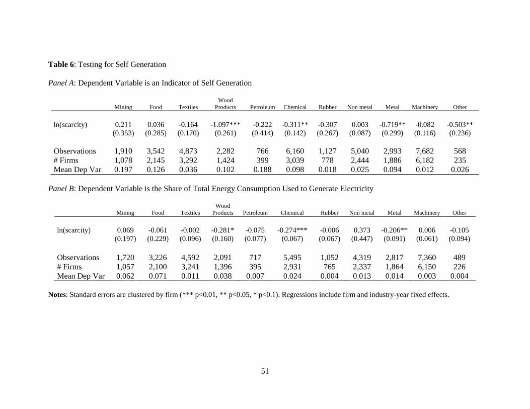
51

Table 6: Testing for Self Generation Panel A: Dependent Variable is an Indicator of Self Generation

Mining Food Textiles

Wood Products Petroleum Chemical Rubber Non metal Metal Machinery Other

ln(scarcity) 0.211 0.036 -0.164 -1.097*** -0.222 -0.311** -0.307 0.003 -0.719** -0.082 -0.503** (0.353) (0.285) (0.170) (0.261) (0.414) (0.142) (0.267) (0.087) (0.299) (0.116) (0.236) Observations 1,910 3,542 4,873 2,282 766 6,160 1,127 5,040 2,993 7,682 568 # Firms 1,078 2,145 3,292 1,424 399 3,039 778 2,444 1,886 6,182 235 Mean Dep Var 0.197 0.126 0.036 0.102 0.188 0.098 0.018 0.025 0.094 0.012 0.026

Panel B: Dependent Variable is the Share of Total Energy Consumption Used to Generate Electricity

Mining Food Textiles

Wood Products Petroleum Chemical Rubber Non metal Metal Machinery Other

ln(scarcity) 0.069 -0.061 -0.002 -0.281* -0.075 -0.274*** -0.006 0.373 -0.206** 0.006 -0.105 (0.197) (0.229) (0.096) (0.160) (0.077) (0.067) (0.067) (0.447) (0.091) (0.061) (0.094) Observations 1,720 3,226 4,592 2,091 717 5,495 1,052 4,319 2,817 7,360 489 # Firms 1,057 2,100 3,241 1,396 395 2,931 765 2,337 1,864 6,150 226 Mean Dep Var 0.062 0.071 0.011 0.038 0.007 0.024 0.004 0.013 0.014 0.003 0.004

Notes: Standard errors are clustered by firm (*** p<0.01, ** p<0.05, * p<0.1). Regressions include firm and industry-year fixed effects.

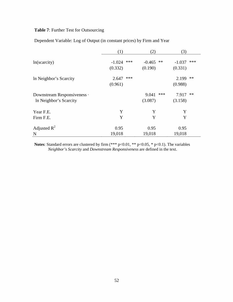
52

Table 7: Further Test for Outsourcing Dependent Variable: Log of Output (in constant prices) by Firm and Year

(1) (2) (3)

ln(scarcity) -1.024 *** -0.465 ** -1.037 ***

(0.332)

(0.190)

(0.331)

ln Neighbor’s Scarcity 2.647 ***

2.199 **

(0.961)

(0.988)

Downstream Responsiveness ∙

9.041 *** 7.917 **

ln Neighbor’s Scarcity

(3.087)

(3.158)

Year F.E. Y

Y

Y Firm F.E. Y

Y

Y

Adjusted R2

0.95

0.95

0.95

N 19,018 19,018 19,018 Notes: Standard errors are clustered by firm (*** p<0.01, ** p<0.05, * p<0.1). The variables

Neighbor’s Scarcity and Downstream Responsiveness are defined in the text.

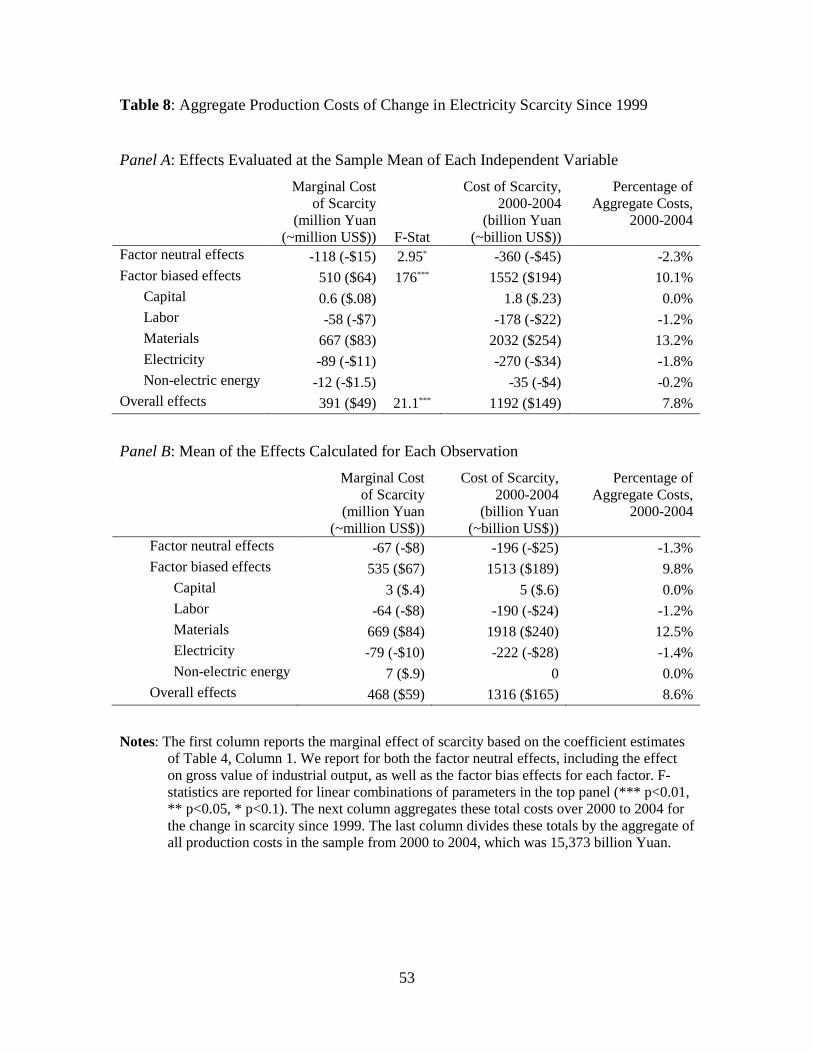
53

Table 8: Aggregate Production Costs of Change in Electricity Scarcity Since 1999

Panel A: Effects Evaluated at the Sample Mean of Each Independent Variable Marginal Cost

of Scarcity (million Yuan

(~million US$)) F-Stat

Cost of Scarcity, 2000-2004

(billion Yuan (~billion US$))

Percentage of Aggregate Costs,

2000-2004

Factor neutral effects -118 (-$15) 2.95* -360 (-$45) -2.3% Factor biased effects 510 ($64) 176*** 1552 ($194) 10.1%

Capital 0.6 ($.08) 1.8 ($.23) 0.0% Labor -58 (-$7) -178 (-$22) -1.2% Materials 667 ($83) 2032 ($254) 13.2% Electricity -89 (-$11) -270 (-$34) -1.8% Non-electric energy -12 (-$1.5) -35 (-$4) -0.2%

Overall effects 391 ($49) 21.1*** 1192 ($149) 7.8%

Panel B: Mean of the Effects Calculated for Each Observation Marginal Cost

of Scarcity (million Yuan

(~million US$))

Cost of Scarcity, 2000-2004

(billion Yuan (~billion US$))

Percentage of Aggregate Costs,

2000-2004

Factor neutral effects -67 (-$8) -196 (-$25) -1.3% Factor biased effects 535 ($67) 1513 ($189) 9.8%

Capital 3 ($.4) 5 ($.6) 0.0% Labor -64 (-$8) -190 (-$24) -1.2% Materials 669 ($84) 1918 ($240) 12.5% Electricity -79 (-$10) -222 (-$28) -1.4% Non-electric energy 7 ($.9) 0 0.0%

Overall effects 468 ($59) 1316 ($165) 8.6%

Notes: The first column reports the marginal effect of scarcity based on the coefficient estimates of Table 4, Column 1. We report for both the factor neutral effects, including the effect on gross value of industrial output, as well as the factor bias effects for each factor. F-statistics are reported for linear combinations of parameters in the top panel (*** p<0.01, ** p<0.05, * p<0.1). The next column aggregates these total costs over 2000 to 2004 for the change in scarcity since 1999. The last column divides these totals by the aggregate of all production costs in the sample from 2000 to 2004, which was 15,373 billion Yuan.

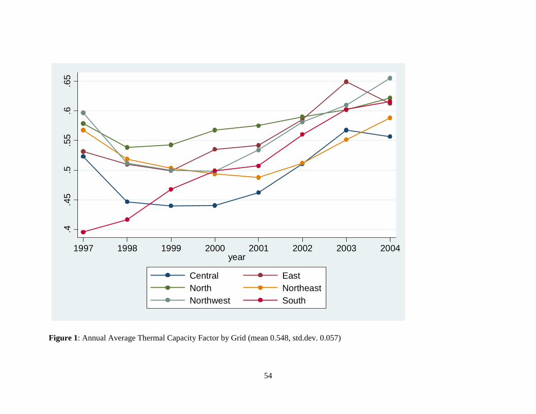
54

Figure 1: Annual Average Thermal Capacity Factor by Grid (mean 0.548, std.dev. 0.057)

.4.4

5.5

.55

.6.6

5

1997 1998 1999 2000 2001 2002 2003 2004year

Central EastNorth NortheastNorthwest South

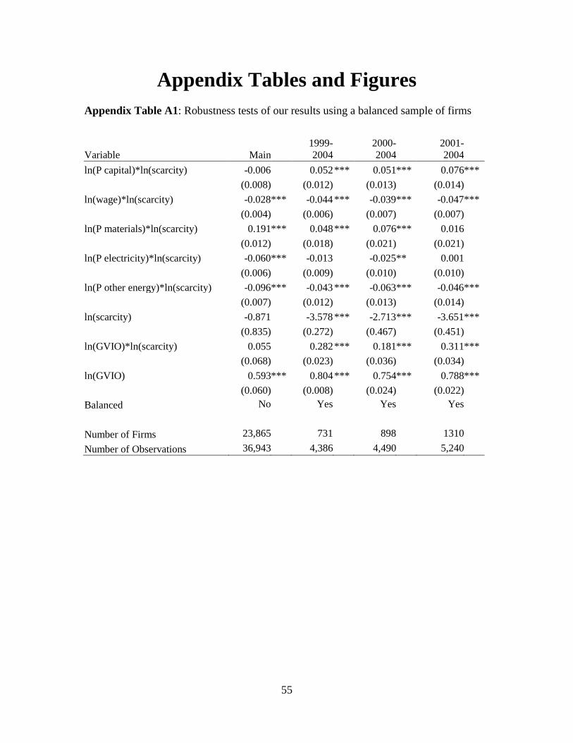
55

Appendix Tables and Figures Appendix Table A1: Robustness tests of our results using a balanced sample of firms

Variable Main 1999-2004

2000-2004

2001- 2004

ln(P capital)*ln(scarcity) -0.006 0.052 *** 0.051 *** 0.076 *** (0.008) (0.012) (0.013) (0.014) ln(wage)*ln(scarcity) -0.028 *** -0.044 *** -0.039 *** -0.047 *** (0.004) (0.006) (0.007) (0.007) ln(P materials)*ln(scarcity) 0.191 *** 0.048 *** 0.076 *** 0.016 (0.012) (0.018) (0.021) (0.021) ln(P electricity)*ln(scarcity) -0.060 *** -0.013 -0.025 ** 0.001 (0.006) (0.009) (0.010) (0.010) ln(P other energy)*ln(scarcity) -0.096 *** -0.043 *** -0.063 *** -0.046 *** (0.007) (0.012) (0.013) (0.014) ln(scarcity) -0.871 -3.578 *** -2.713 *** -3.651 *** (0.835) (0.272) (0.467) (0.451) ln(GVIO)*ln(scarcity) 0.055 0.282 *** 0.181 *** 0.311 *** (0.068) (0.023) (0.036) (0.034) ln(GVIO) 0.593 *** 0.804 *** 0.754 *** 0.788 *** (0.060) (0.008) (0.024) (0.022) Balanced No Yes Yes Yes Number of Firms 23,865 731 898 1310 Number of Observations 36,943 4,386 4,490 5,240

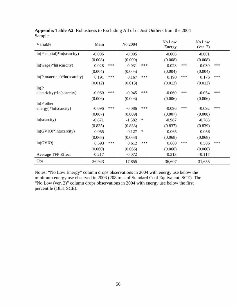
56

Appendix Table A2: Robustness to Excluding All of or Just Outliers from the 2004 Sample

Variable Main No 2004 No Low Energy No Low

(ver. 2)

ln(P capital)*ln(scarcity) -0.006

-0.005

-0.006

-0.001

(0.008)

(0.009)

(0.008)

(0.008) ln(wage)*ln(scarcity) -0.028 *** -0.031 *** -0.028 *** -0.030 ***

(0.004)

(0.005)

(0.004)

(0.004) ln(P materials)*ln(scarcity) 0.191 *** 0.167 *** 0.190 *** 0.176 ***

(0.012)

(0.013)

(0.012)

(0.012) ln(P

electricity)*ln(scarcity) -0.060 *** -0.045 *** -0.060 *** -0.054 ***

(0.006)

(0.008)

(0.006)

(0.006) ln(P other

energy)*ln(scarcity) -0.096 *** -0.086 *** -0.096 *** -0.092 ***

(0.007)

(0.009)

(0.007)

(0.008) ln(scarcity) -0.871

-1.582 * -0.987

-0.788

(0.835)

(0.833)

(0.837)

(0.839)

ln(GVIO)*ln(scarcity) 0.055

0.127 * 0.065

0.056

(0.068)

(0.068)

(0.068)

(0.068) ln(GVIO) 0.593 *** 0.612 *** 0.600 *** 0.586 ***

(0.060)

(0.066)

(0.060)

(0.060) Average TFP Effect -0.217 -0.072 -0.213 -0.117

Obs 36,943 17,855 36,607 31,655 Notes: “No Low Energy” column drops observations in 2004 with energy use below the minimum energy use observed in 2003 (208 tons of Standard Coal Equivalent, SCE). The “No Low (ver. 2)” column drops observations in 2004 with energy use below the first percentile (1851 SCE).

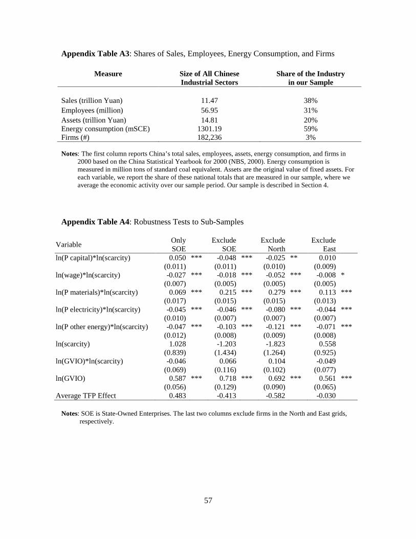
57

Appendix Table A3: Shares of Sales, Employees, Energy Consumption, and Firms

Measure Size of All Chinese Industrial Sectors

Share of the Industry in our Sample

Sales (trillion Yuan) 11.47 38% Employees (million) 56.95 31% Assets (trillion Yuan) 14.81 20% Energy consumption (mSCE) 1301.19 59% Firms (#) 182,236 3% Notes: The first column reports China’s total sales, employees, assets, energy consumption, and firms in

2000 based on the China Statistical Yearbook for 2000 (NBS, 2000). Energy consumption is measured in million tons of standard coal equivalent. Assets are the original value of fixed assets. For each variable, we report the share of these national totals that are measured in our sample, where we average the economic activity over our sample period. Our sample is described in Section 4.

Appendix Table A4: Robustness Tests to Sub-Samples

Variable Only SOE Exclude

SOE Exclude North Exclude

East

ln(P capital)*ln(scarcity) 0.050 *** -0.048 *** -0.025 ** 0.010 (0.011) (0.011) (0.010) (0.009) ln(wage)*ln(scarcity) -0.027 *** -0.018 *** -0.052 *** -0.008 * (0.007) (0.005) (0.005) (0.005) ln(P materials)*ln(scarcity) 0.069 *** 0.215 *** 0.279 *** 0.113 *** (0.017) (0.015) (0.015) (0.013) ln(P electricity)*ln(scarcity) -0.045 *** -0.046 *** -0.080 *** -0.044 *** (0.010) (0.007) (0.007) (0.007) ln(P other energy)*ln(scarcity) -0.047 *** -0.103 *** -0.121 *** -0.071 *** (0.012) (0.008) (0.009) (0.008) ln(scarcity) 1.028 -1.203 -1.823 0.558 (0.839) (1.434) (1.264) (0.925) ln(GVIO)*ln(scarcity) -0.046 0.066 0.104 -0.049 (0.069) (0.116) (0.102) (0.077) ln(GVIO) 0.587 *** 0.718 *** 0.692 *** 0.561 *** (0.056) (0.129) (0.090) (0.065) Average TFP Effect 0.483 -0.413 -0.582 -0.030

Notes: SOE is State-Owned Enterprises. The last two columns exclude firms in the North and East grids,

respectively.

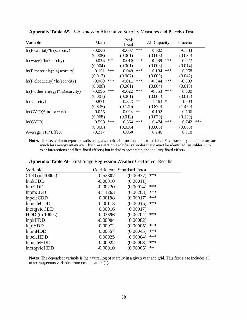
58

Appendix Table A5: Robustness to Alternative Scarcity Measures and Placebo Test

Variable Main Peak Load All Capacity Placebo

ln(P capital)*ln(scarcity) -0.006 -0.007 *** 0.002 -0.033 (0.008) (0.001) (0.006) (0.030) ln(wage)*ln(scarcity) -0.028 *** -0.010 *** -0.039 *** -0.022 (0.004) (0.001) (0.003) (0.014) ln(P materials)*ln(scarcity) 0.191 *** 0.049 *** 0.134 *** 0.058 (0.012) (0.002) (0.009) (0.042) ln(P electricity)*ln(scarcity) -0.060 *** -0.011 *** -0.044 *** -0.003 (0.006) (0.001) (0.004) (0.010) ln(P other energy)*ln(scarcity) -0.096 *** -0.022 *** -0.053 *** 0.000 (0.007) (0.001) (0.005) (0.012) ln(scarcity) -0.871 0.343 ** 1.463 * -1.499 (0.835) (0.149) (0.870) (1.420) ln(GVIO)*ln(scarcity) 0.055 -0.024 ** -0.102 0.136 (0.068) (0.012) (0.070) (0.120) ln(GVIO) 0.593 *** 0.564 *** 0.474 *** 0.742 *** (0.060) (0.036) (0.065) (0.060) Average TFP Effect -0.217 0.060 0.246 0.118

Notes: The last column reports results using a sample of firms that appear in the 2004 census only and therefore are

much less energy intensive. This cross section excludes variables that cannot be identified (variables with year interactions and firm fixed effects) but includes ownership and industry fixed effects.

Appendix Table A6: First-Stage Regression Weather Coefficient Results

Variable Coefficient Standard Error CDD (in 1000s) 0.52807 (0.00937) *** lnpkCDD -0.00010 (0.00011) lnplCDD -0.00220 (0.00024) *** lnpmCDD -0.11263 (0.00203) *** lnpeleCDD 0.00198 (0.00017) *** lnpneleCDD -0.00113 (0.00015) *** lncstgvioCDD 0.00016 (0.00017) HDD (in 1000s) 0.03696 (0.00204) *** lnpkHDD -0.00004 (0.00002) lnplHDD -0.00072 (0.00005) *** lnpmHDD -0.00557 (0.00045) *** lnpeleHDD 0.00025 (0.00004) *** lnpneleHDD -0.00022 (0.00003) *** lncstgvioHDD -0.00010 (0.00005) **

Notes: The dependent variable is the natural log of scarcity in a given year and grid. This first stage includes all other exogenous variables from cost equation (1).

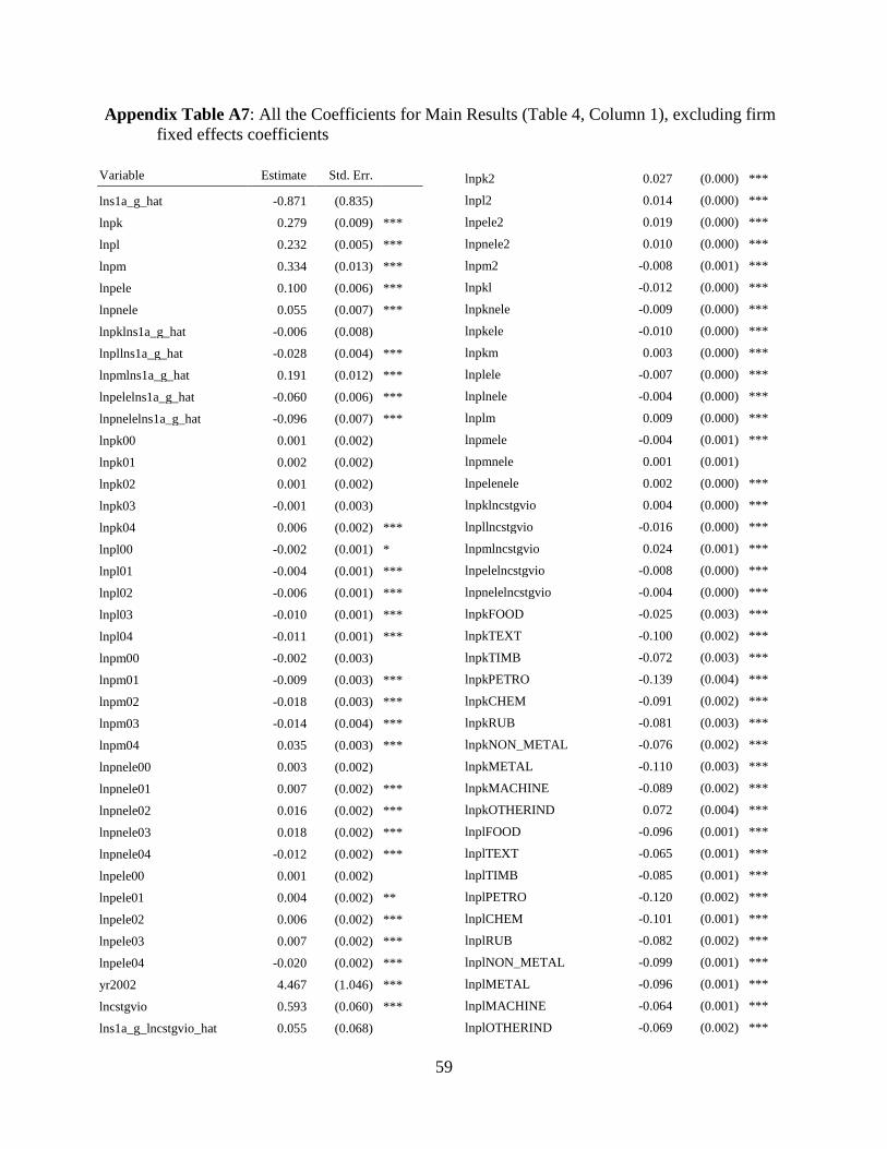
59

Appendix Table A7: All the Coefficients for Main Results (Table 4, Column 1), excluding firm fixed effects coefficients

Variable Estimate Std. Err. lns1a_g_hat -0.871 (0.835)

lnpk 0.279 (0.009) ***

lnpl 0.232 (0.005) ***

lnpm 0.334 (0.013) ***

lnpele 0.100 (0.006) ***

lnpnele 0.055 (0.007) ***

lnpklns1a_g_hat -0.006 (0.008) lnpllns1a_g_hat -0.028 (0.004) ***

lnpmlns1a_g_hat 0.191 (0.012) ***

lnpelelns1a_g_hat -0.060 (0.006) ***

lnpnelelns1a_g_hat -0.096 (0.007) ***

lnpk00 0.001 (0.002)

lnpk01 0.002 (0.002)

lnpk02 0.001 (0.002) lnpk03 -0.001 (0.003) lnpk04 0.006 (0.002) ***

lnpl00 -0.002 (0.001) *

lnpl01 -0.004 (0.001) ***

lnpl02 -0.006 (0.001) ***

lnpl03 -0.010 (0.001) ***

lnpl04 -0.011 (0.001) ***

lnpm00 -0.002 (0.003) lnpm01 -0.009 (0.003) ***

lnpm02 -0.018 (0.003) ***

lnpm03 -0.014 (0.004) ***

lnpm04 0.035 (0.003) ***

lnpnele00 0.003 (0.002) lnpnele01 0.007 (0.002) ***

lnpnele02 0.016 (0.002) ***

lnpnele03 0.018 (0.002) ***

lnpnele04 -0.012 (0.002) ***

lnpele00 0.001 (0.002) lnpele01 0.004 (0.002) **

lnpele02 0.006 (0.002) ***

lnpele03 0.007 (0.002) ***

lnpele04 -0.020 (0.002) ***

yr2002 4.467 (1.046) ***

lncstgvio 0.593 (0.060) ***

lns1a_g_lncstgvio_hat 0.055 (0.068)

lnpk2 0.027 (0.000) ***

lnpl2 0.014 (0.000) ***

lnpele2 0.019 (0.000) ***

lnpnele2 0.010 (0.000) ***

lnpm2 -0.008 (0.001) ***

lnpkl -0.012 (0.000) ***

lnpknele -0.009 (0.000) ***

lnpkele -0.010 (0.000) ***

lnpkm 0.003 (0.000) ***

lnplele -0.007 (0.000) ***

lnplnele -0.004 (0.000) ***

lnplm 0.009 (0.000) ***

lnpmele -0.004 (0.001) ***

lnpmnele 0.001 (0.001) lnpelenele 0.002 (0.000) ***

lnpklncstgvio 0.004 (0.000) ***

lnpllncstgvio -0.016 (0.000) ***

lnpmlncstgvio 0.024 (0.001) ***

lnpelelncstgvio -0.008 (0.000) ***

lnpnelelncstgvio -0.004 (0.000) ***

lnpkFOOD -0.025 (0.003) ***

lnpkTEXT -0.100 (0.002) ***

lnpkTIMB -0.072 (0.003) ***

lnpkPETRO -0.139 (0.004) ***

lnpkCHEM -0.091 (0.002) ***

lnpkRUB -0.081 (0.003) ***

lnpkNON_METAL -0.076 (0.002) ***

lnpkMETAL -0.110 (0.003) ***

lnpkMACHINE -0.089 (0.002) ***

lnpkOTHERIND 0.072 (0.004) ***

lnplFOOD -0.096 (0.001) ***

lnplTEXT -0.065 (0.001) ***

lnplTIMB -0.085 (0.001) ***

lnplPETRO -0.120 (0.002) ***

lnplCHEM -0.101 (0.001) ***

lnplRUB -0.082 (0.002) ***

lnplNON_METAL -0.099 (0.001) ***

lnplMETAL -0.096 (0.001) ***

lnplMACHINE -0.064 (0.001) ***

lnplOTHERIND -0.069 (0.002) ***

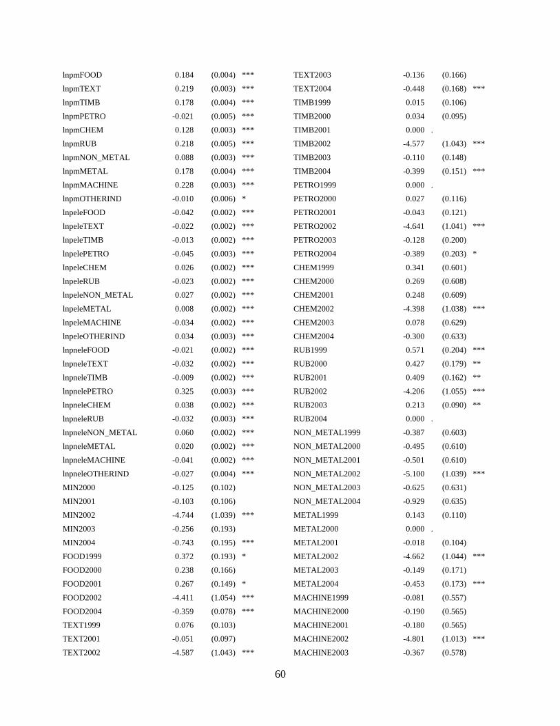
60

lnpmFOOD 0.184 (0.004) ***

lnpmTEXT 0.219 (0.003) ***

lnpmTIMB 0.178 (0.004) ***

lnpmPETRO -0.021 (0.005) ***

lnpmCHEM 0.128 (0.003) ***

lnpmRUB 0.218 (0.005) ***

lnpmNON_METAL 0.088 (0.003) ***

lnpmMETAL 0.178 (0.004) ***

lnpmMACHINE 0.228 (0.003) ***

lnpmOTHERIND -0.010 (0.006) *

lnpeleFOOD -0.042 (0.002) ***

lnpeleTEXT -0.022 (0.002) ***

lnpeleTIMB -0.013 (0.002) ***

lnpelePETRO -0.045 (0.003) ***

lnpeleCHEM 0.026 (0.002) ***

lnpeleRUB -0.023 (0.002) ***

lnpeleNON_METAL 0.027 (0.002) ***

lnpeleMETAL 0.008 (0.002) ***

lnpeleMACHINE -0.034 (0.002) ***

lnpeleOTHERIND 0.034 (0.003) ***

lnpneleFOOD -0.021 (0.002) ***

lnpneleTEXT -0.032 (0.002) ***

lnpneleTIMB -0.009 (0.002) ***

lnpnelePETRO 0.325 (0.003) ***

lnpneleCHEM 0.038 (0.002) ***

lnpneleRUB -0.032 (0.003) ***

lnpneleNON_METAL 0.060 (0.002) ***

lnpneleMETAL 0.020 (0.002) ***

lnpneleMACHINE -0.041 (0.002) ***

lnpneleOTHERIND -0.027 (0.004) ***

MIN2000 -0.125 (0.102) MIN2001 -0.103 (0.106) MIN2002 -4.744 (1.039) ***

MIN2003 -0.256 (0.193) MIN2004 -0.743 (0.195) ***

FOOD1999 0.372 (0.193) *

FOOD2000 0.238 (0.166) FOOD2001 0.267 (0.149) *

FOOD2002 -4.411 (1.054) ***

FOOD2004 -0.359 (0.078) ***

TEXT1999 0.076 (0.103) TEXT2001 -0.051 (0.097) TEXT2002 -4.587 (1.043) ***

TEXT2003 -0.136 (0.166) TEXT2004 -0.448 (0.168) ***

TIMB1999 0.015 (0.106) TIMB2000 0.034 (0.095) TIMB2001 0.000 . TIMB2002 -4.577 (1.043) ***

TIMB2003 -0.110 (0.148) TIMB2004 -0.399 (0.151) ***

PETRO1999 0.000 . PETRO2000 0.027 (0.116) PETRO2001 -0.043 (0.121) PETRO2002 -4.641 (1.041) ***

PETRO2003 -0.128 (0.200) PETRO2004 -0.389 (0.203) *

CHEM1999 0.341 (0.601) CHEM2000 0.269 (0.608) CHEM2001 0.248 (0.609) CHEM2002 -4.398 (1.038) ***

CHEM2003 0.078 (0.629) CHEM2004 -0.300 (0.633) RUB1999 0.571 (0.204) ***

RUB2000 0.427 (0.179) **

RUB2001 0.409 (0.162) **

RUB2002 -4.206 (1.055) ***

RUB2003 0.213 (0.090) **

RUB2004 0.000 . NON_METAL1999 -0.387 (0.603) NON_METAL2000 -0.495 (0.610) NON_METAL2001 -0.501 (0.610) NON_METAL2002 -5.100 (1.039) ***

NON_METAL2003 -0.625 (0.631) NON_METAL2004 -0.929 (0.635) METAL1999 0.143 (0.110) METAL2000 0.000 . METAL2001 -0.018 (0.104) METAL2002 -4.662 (1.044) ***

METAL2003 -0.149 (0.171) METAL2004 -0.453 (0.173) ***

MACHINE1999 -0.081 (0.557) MACHINE2000 -0.190 (0.565) MACHINE2001 -0.180 (0.565) MACHINE2002 -4.801 (1.013) ***

MACHINE2003 -0.367 (0.578)

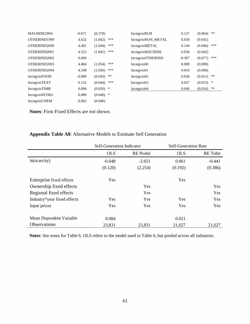
61

MACHINE2004 -0.671 (0.578) OTHERIND1999 4.632 (1.042) ***

OTHERIND2000 4.481 (1.044) ***

OTHERIND2001 4.523 (1.041) ***

OTHERIND2002 0.000 . OTHERIND2003 4.466 (1.054) ***

OTHERIND2004 4.198 (1.056) ***

lncstgvioFOOD -0.090 (0.043) **

lncstgvioTEXT 0.131 (0.044) ***

lncstgvioTIMB 0.096 (0.050) *

lncstgvioPETRO 0.089 (0.049) *

lncstgvioCHEM 0.062 (0.040)

lncstgvioRUB 0.127 (0.064) **

lncstgvioNON_METAL 0.030 (0.041) lncstgvioMETAL 0.144 (0.046) ***

lncstgvioMACHINE 0.034 (0.042) lncstgvioOTHERIND -0.307 (0.077) ***

lncstgvio00 0.008 (0.008) lncstgvio01 0.010 (0.008) lncstgvio02 0.026 (0.011) **

lncstgvio03 0.027 (0.015) *

lncstgvio04 0.040 (0.016) **

Notes: Firm Fixed Effects are not shown.

Appendix Table A8: Alternative Models to Estimate Self Generation

Self-Generation Indicator Self-Generation Rate

OLS RE Probit OLS RE Tobit ln(scarcity) -0.048 -2.651 0.061 -0.441

(0.120) (2.254) (0.192) (0.386)

Enterprise fixed effects Yes

Yes Ownership fixed effects

Yes

Yes

Regional fixed effects

Yes

Yes Industry*year fixed effects Yes Yes Yes Yes Input prices Yes Yes Yes Yes

Mean Dependent Variable 0.084

0.021 Observations 23,831 23,831 21,627 21,627

Notes: See notes for Table 6. OLS refers to the model used in Table 6, but pooled across all industries.

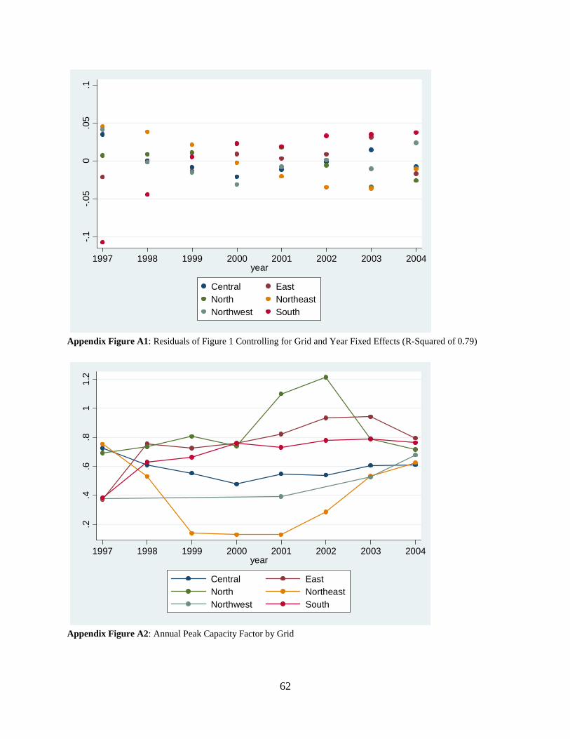
62

Appendix Figure A1: Residuals of Figure 1 Controlling for Grid and Year Fixed Effects (R-Squared of 0.79)

Appendix Figure A2: Annual Peak Capacity Factor by Grid

-.1-.0

50

.05

.1

1997 1998 1999 2000 2001 2002 2003 2004year

Central EastNorth NortheastNorthwest South

.2.4

.6.8

11.

2

1997 1998 1999 2000 2001 2002 2003 2004year

Central EastNorth NortheastNorthwest South

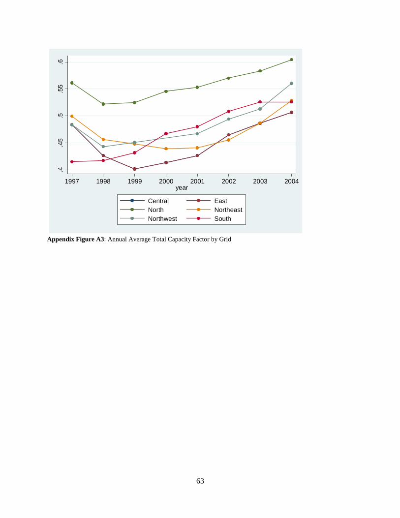
63

Appendix Figure A3: Annual Average Total Capacity Factor by Grid

.4.4

5.5

.55

.6

1997 1998 1999 2000 2001 2002 2003 2004year

Central EastNorth NortheastNorthwest South