Embed Size (px)
Citation preview
Electronic Structure Theory in Practice
Oliver T. Hofmann, Trieste, Aug 7th 2013
1
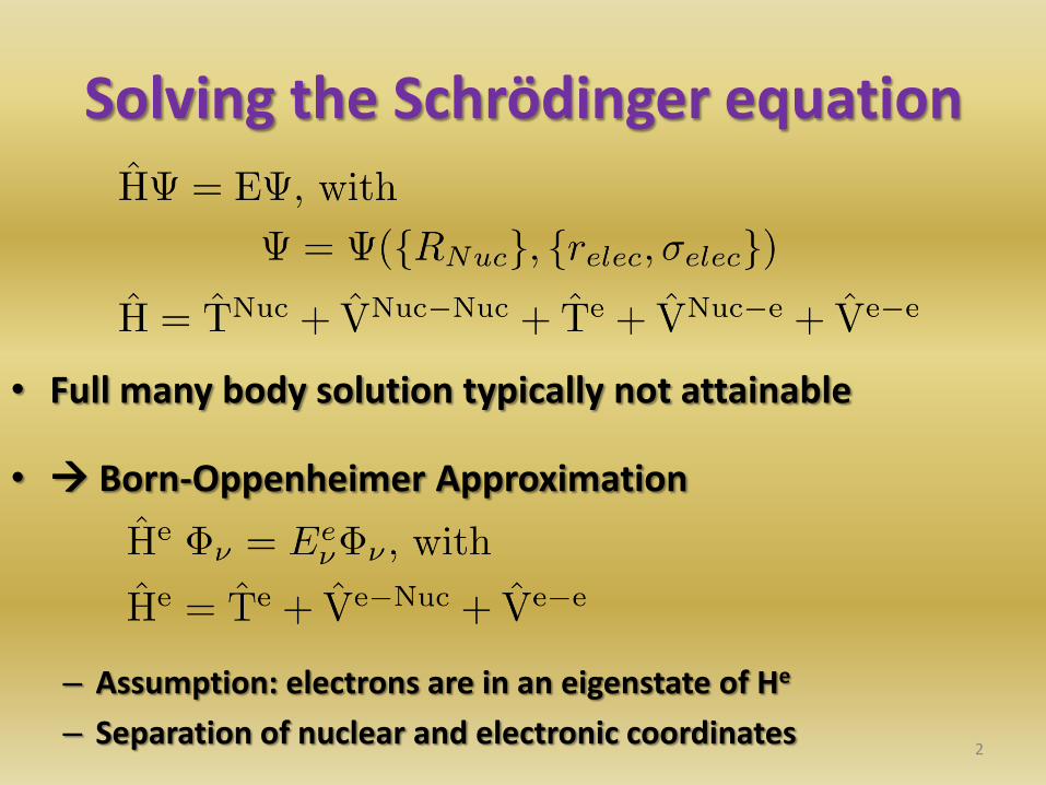
Solving the Schrödinger equation
2
• Full many body solution typically not attainable
• Born-Oppenheimer Approximation
– Assumption: electrons are in an eigenstate of He
– Separation of nuclear and electronic coordinates
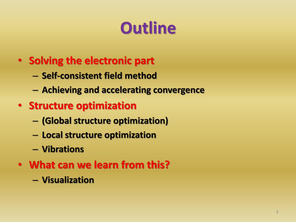
Outline
• Solving the electronic part
– Self-consistent field method
– Achieving and accelerating convergence
• Structure optimization
– (Global structure optimization)
– Local structure optimization
– Vibrations
• What can we learn from this?
– Visualization
3
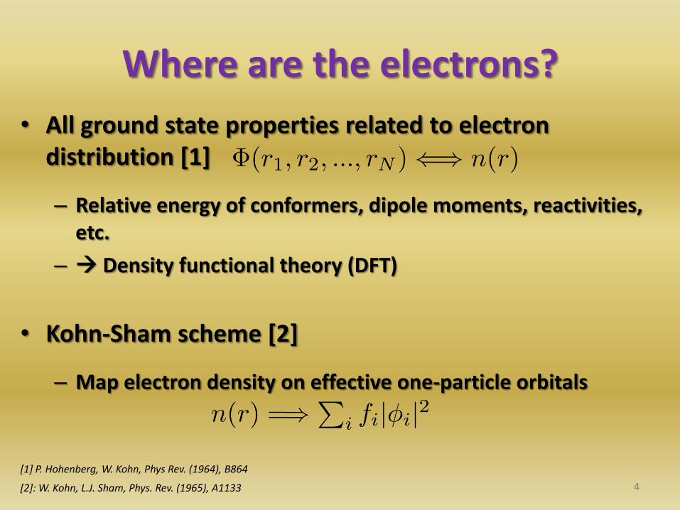
Where are the electrons?
• All ground state properties related to electron distribution [1]
– Relative energy of conformers, dipole moments, reactivities, etc.
– Density functional theory (DFT)
• Kohn-Sham scheme [2]
– Map electron density on effective one-particle orbitals
4
[1] P. Hohenberg, W. Kohn, Phys Rev. (1964), B864
[2]: W. Kohn, L.J. Sham, Phys. Rev. (1965), A1133
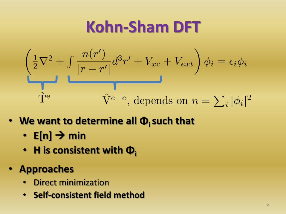
Kohn-Sham DFT
5
• We want to determine all Φi such that
• E[n] min
• H is consistent with Φi
• Approaches • Direct minimization
• Self-consistent field method
6
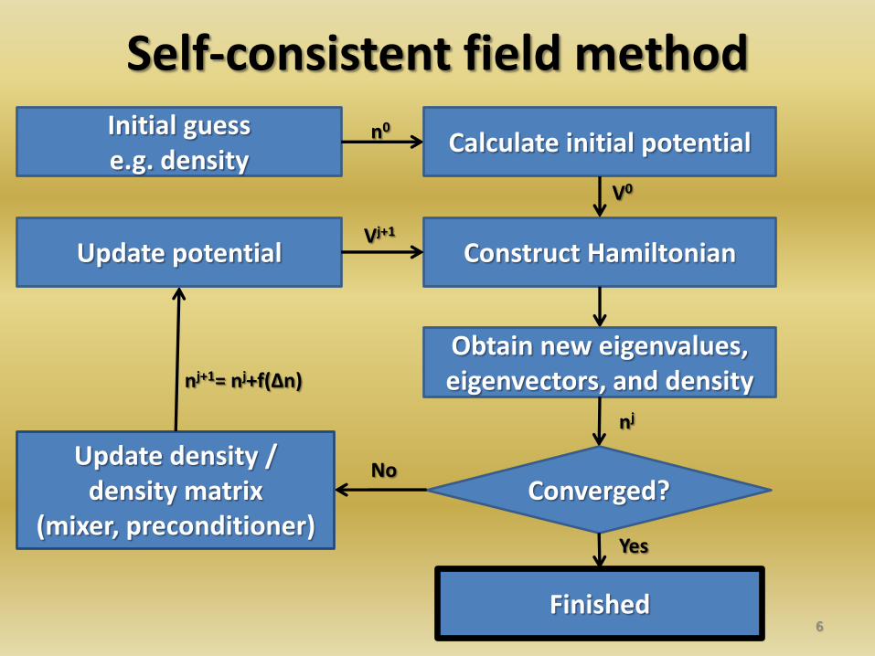
Initial guess e.g. density
Calculate initial potential
Construct Hamiltonian
Obtain new eigenvalues, eigenvectors, and density
Converged? Update density /
density matrix (mixer, preconditioner)
Update potential
Finished
Yes
No
n0
V0
nj
nj+1= nj+f(Δn)
Vj+1
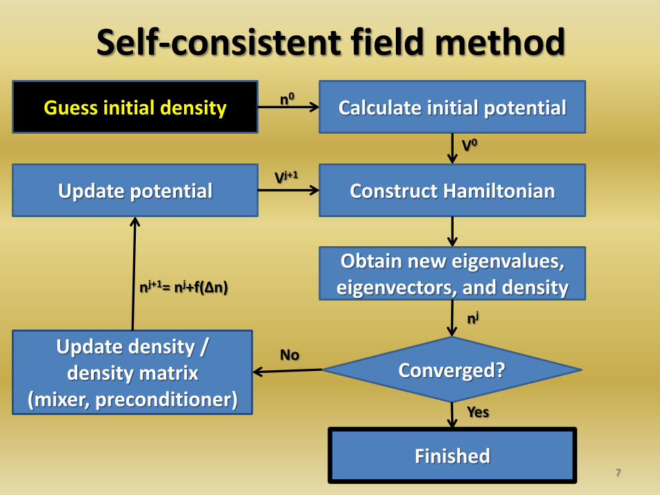
Self-consistent field method
Self-consistent field method
7
Guess initial density Calculate initial potential
Construct Hamiltonian
Obtain new eigenvalues, eigenvectors, and density
Converged? Update density /
density matrix (mixer, preconditioner)
Update potential
Finished
Yes
No
n0
V0
nj
nj+1= nj+f(Δn)
Vj+1
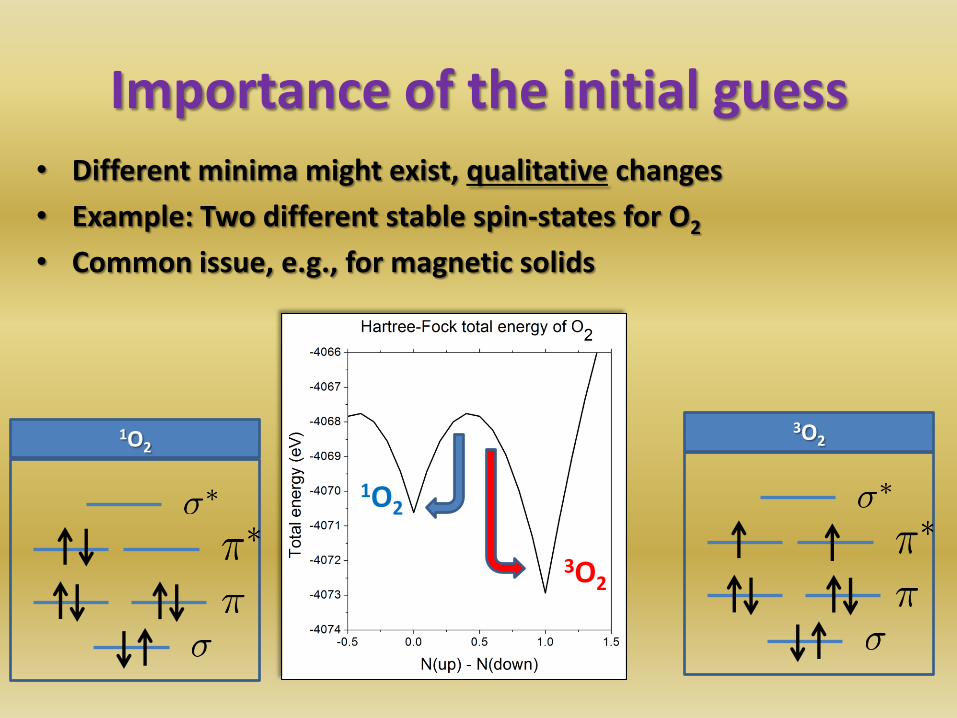
Importance of the initial guess • Different minima might exist, qualitative changes
• Example: Two different stable spin-states for O2
• Common issue, e.g., for magnetic solids
3O2 1O2
1O2
3O2
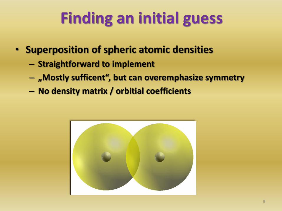
Finding an initial guess
• Superposition of spheric atomic densities
– Straightforward to implement
– „Mostly sufficent“, but can overemphasize symmetry
– No density matrix / orbitial coefficients
9
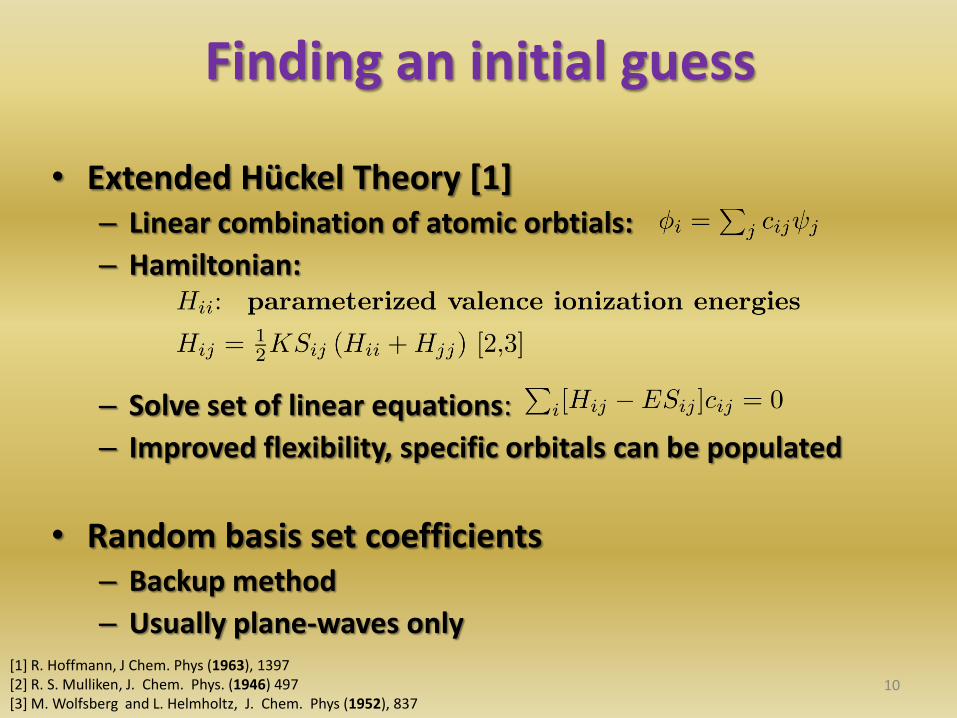
Finding an initial guess
• Extended Hückel Theory [1] – Linear combination of atomic orbtials:
– Hamiltonian:
– Solve set of linear equations:
– Improved flexibility, specific orbitals can be populated
• Random basis set coefficients – Backup method
– Usually plane-waves only
10
[1] R. Hoffmann, J Chem. Phys (1963), 1397 [2] R. S. Mulliken, J. Chem. Phys. (1946) 497 [3] M. Wolfsberg and L. Helmholtz, J. Chem. Phys (1952), 837
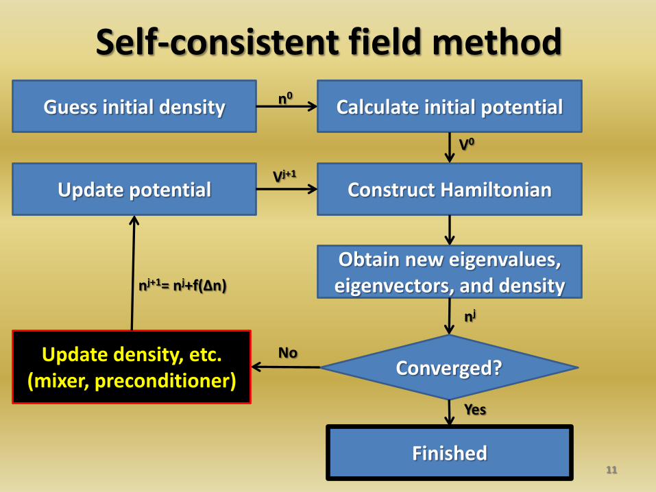
Self-consistent field method
11
Guess initial density Calculate initial potential
Construct Hamiltonian
Obtain new eigenvalues, eigenvectors, and density
Converged? Update density, etc.
(mixer, preconditioner)
Update potential
Finished
Yes
No
n0
V0
nj
nj+1= nj+f(Δn)
Vj+1
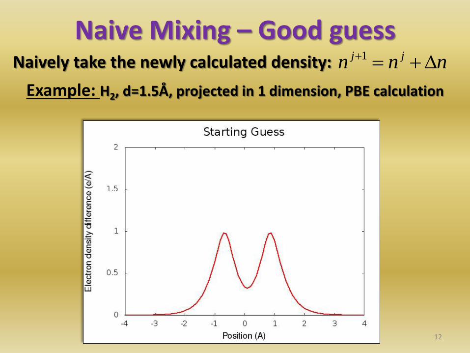
Naive Mixing – Good guess Naively take the newly calculated density:
12
nnn jj 1
Example: H2, d=1.5Å, projected in 1 dimension, PBE calculation
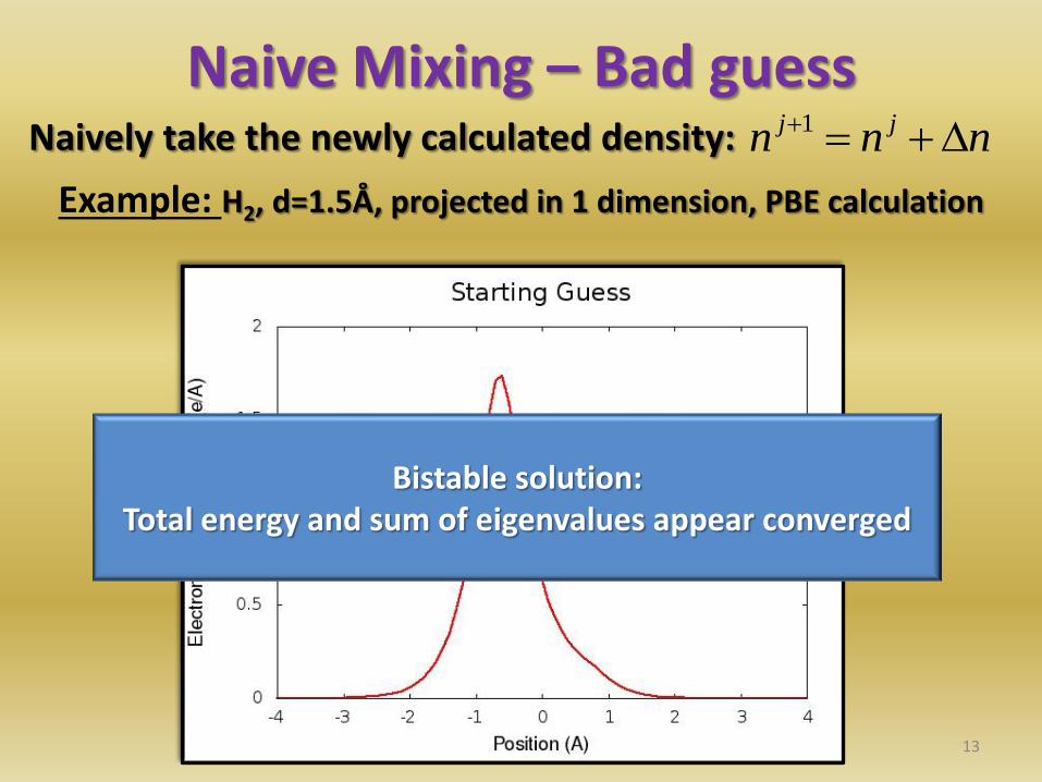
Naive Mixing – Bad guess Naively take the newly calculated density:
13
nnn jj 1
Example: H2, d=1.5Å, projected in 1 dimension, PBE calculation
Bistable solution: Total energy and sum of eigenvalues appear converged
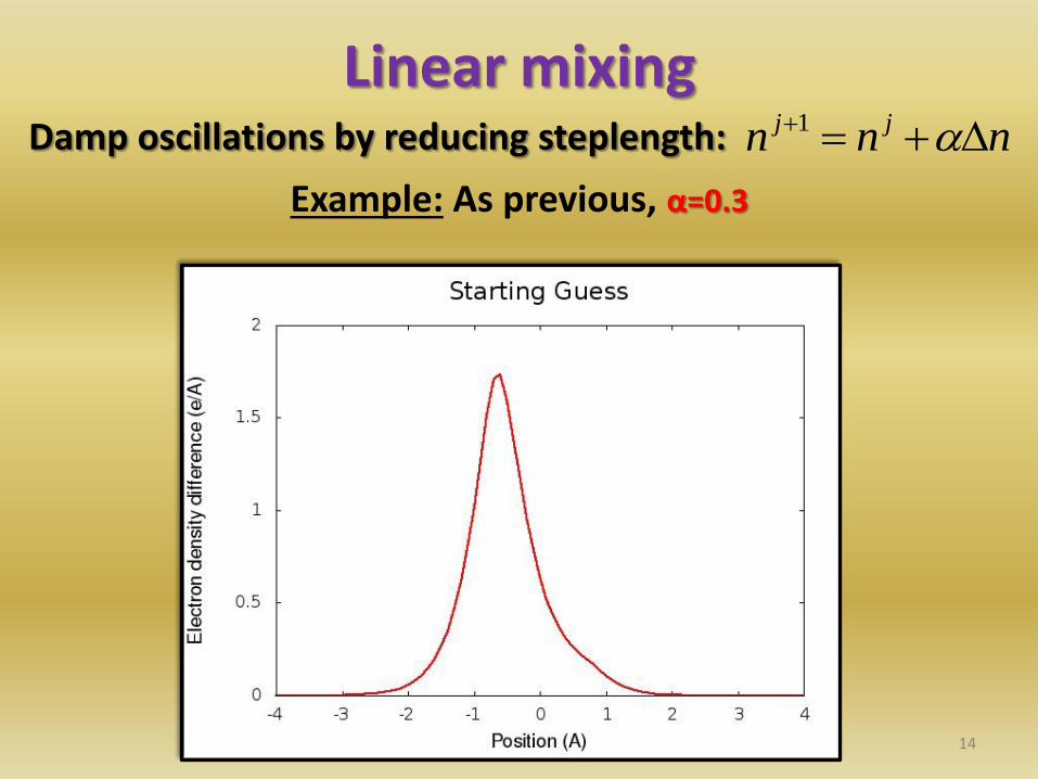
Linear mixing Damp oscillations by reducing steplength:
14
nnn jj 1
Example: As previous, α=0.3
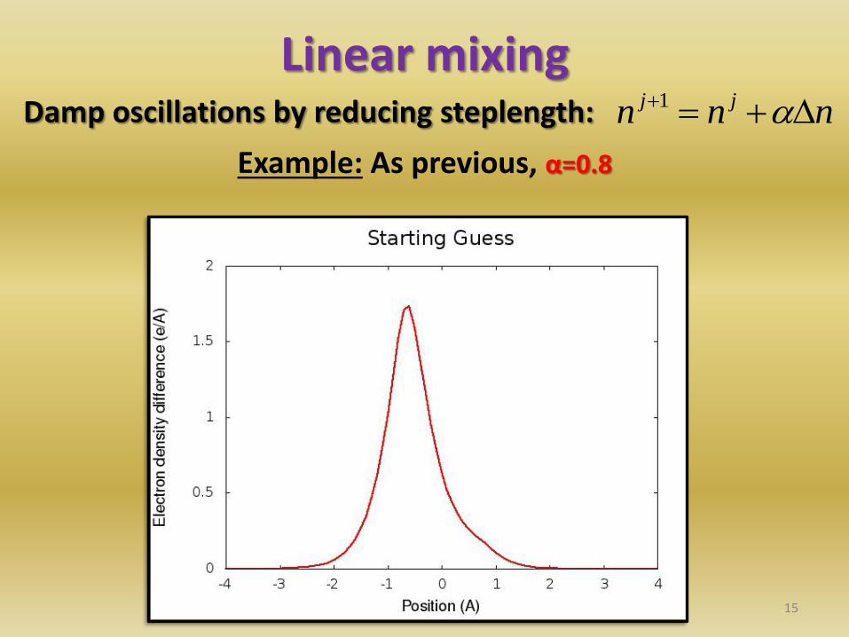
Linear mixing Damp oscillations by reducing steplength:
15
nnn jj 1
Example: As previous, α=0.8
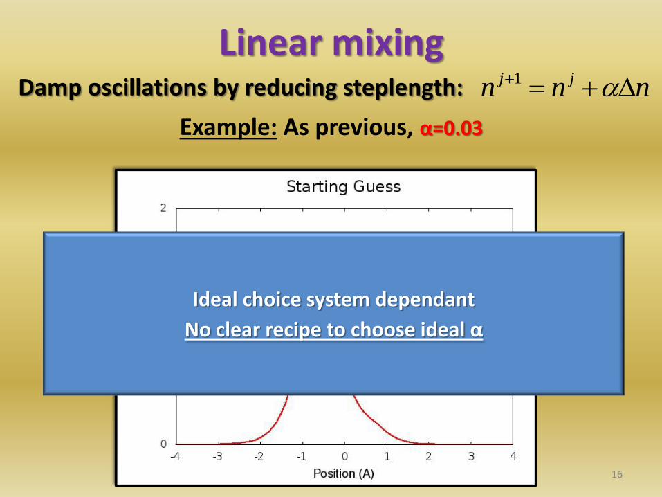
Linear mixing Damp oscillations by reducing steplength:
16
nnn jj 1
Example: As previous, α=0.03
Ideal choice system dependant
No clear recipe to choose ideal α
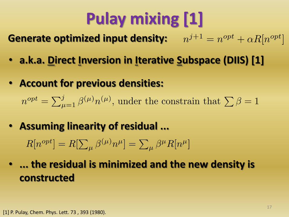
Pulay mixing [1] Generate optimized input density:
17 [1] P. Pulay, Chem. Phys. Lett. 73 , 393 (1980).
• a.k.a. Direct Inversion in Iterative Subspace (DIIS) [1]
• Account for previous densities:
• Assuming linearity of residual ...
• ... the residual is minimized and the new density is constructed
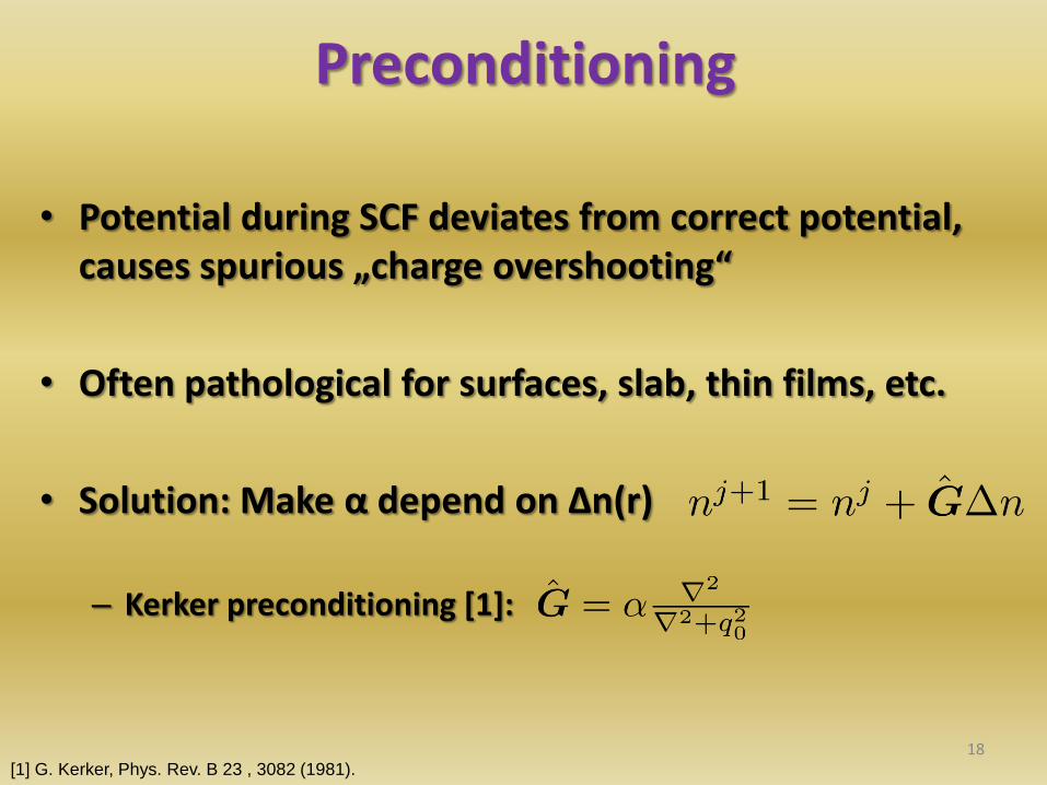
Preconditioning
• Potential during SCF deviates from correct potential, causes spurious „charge overshooting“
• Often pathological for surfaces, slab, thin films, etc.
• Solution: Make α depend on Δn(r)
– Kerker preconditioning [1]:
18 [1] G. Kerker, Phys. Rev. B 23 , 3082 (1981).
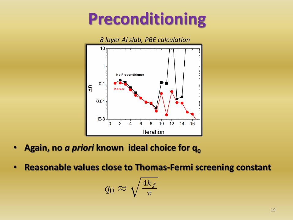
Preconditioning
19
• Again, no a priori known ideal choice for q0
• Reasonable values close to Thomas-Fermi screening constant
8 layer Al slab, PBE calculation
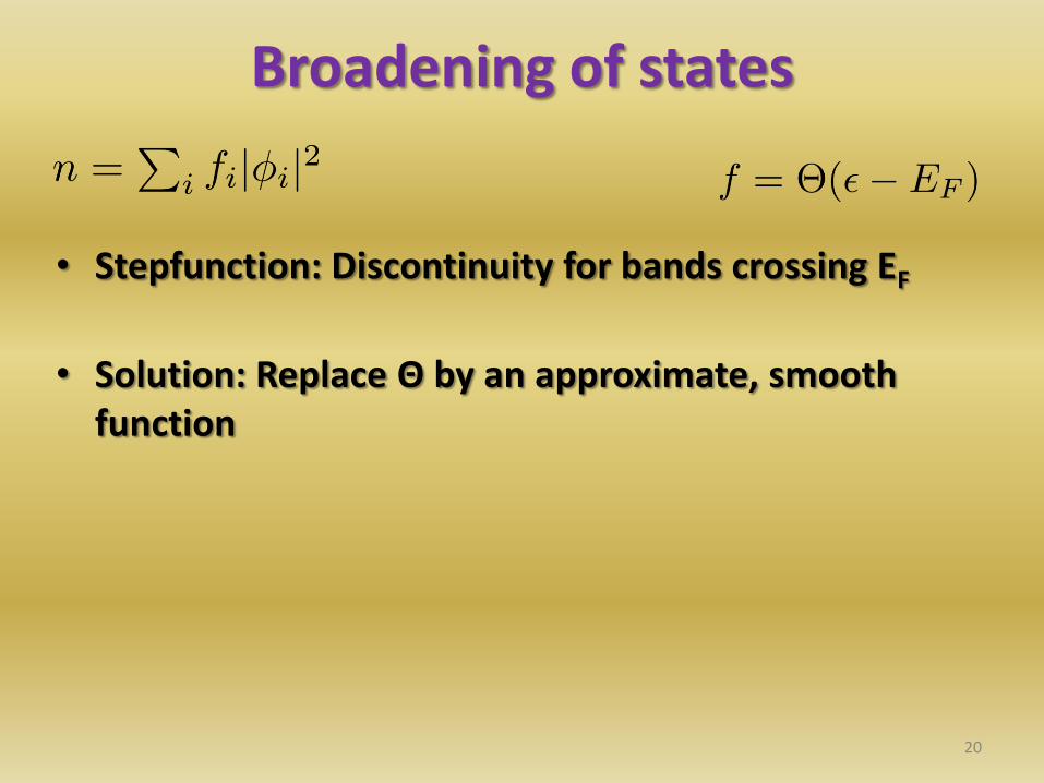
Broadening of states
• Stepfunction: Discontinuity for bands crossing EF
• Solution: Replace Θ by an approximate, smooth function
20
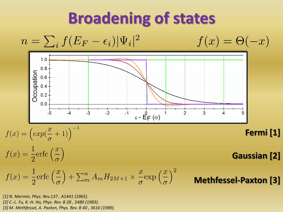
Broadening of states
Methfessel-Paxton [3]
[1] N. Mermin, Phys. Rev.137 , A1441 (1965). [2] C.-L. Fu, K.-H. Ho, Phys. Rev. B 28 , 5480 (1983). [3] M. Methfessel, A. Paxton, Phys. Rev. B 40 , 3616 (1989).
Gaussian [2]
Fermi [1]
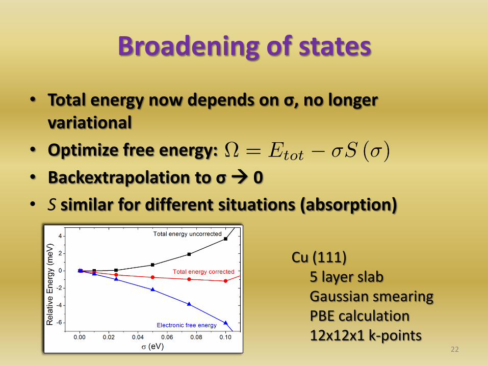
Broadening of states
• Total energy now depends on σ, no longer variational
• Optimize free energy:
• Backextrapolation to σ 0
• S similar for different situations (absorption)
22
Cu (111) 5 layer slab Gaussian smearing PBE calculation 12x12x1 k-points
Summary SCF
• Ground state electron density determined iteratively
• Initial guess needs initial thought, can change results qualiatively
• Density update by – Linear mixing (slow)
– Pulay mixing
• Convergence acceleration by – Preconditioner
– Broadening of states
23
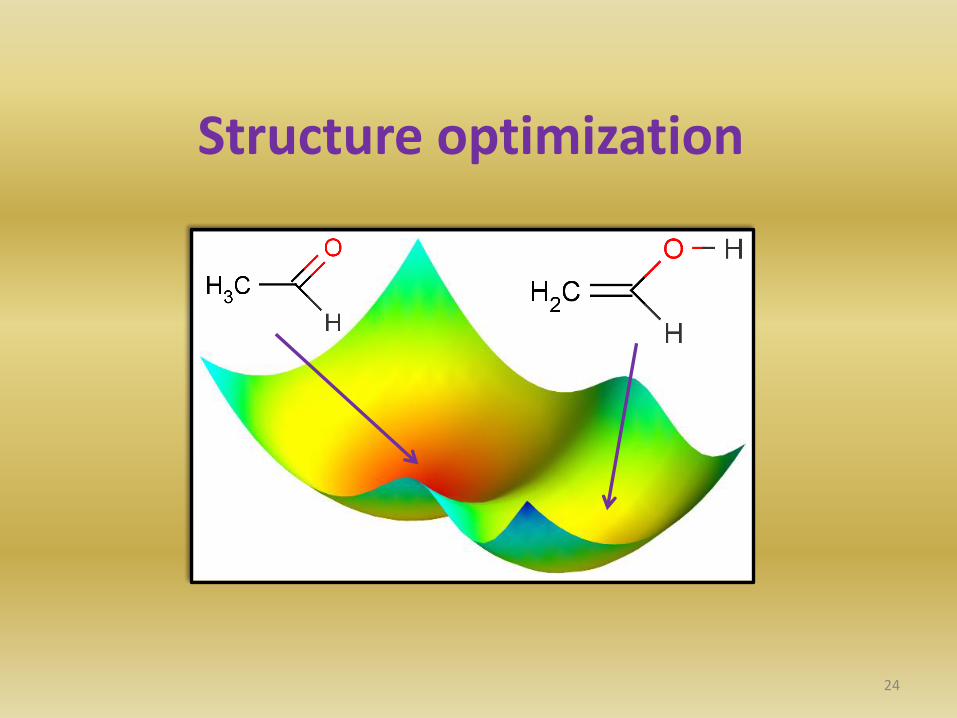
Structure optimization
24
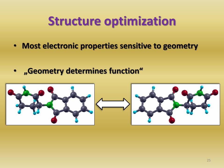
Structure optimization
• Most electronic properties sensitive to geometry
• „Geometry determines function“
25
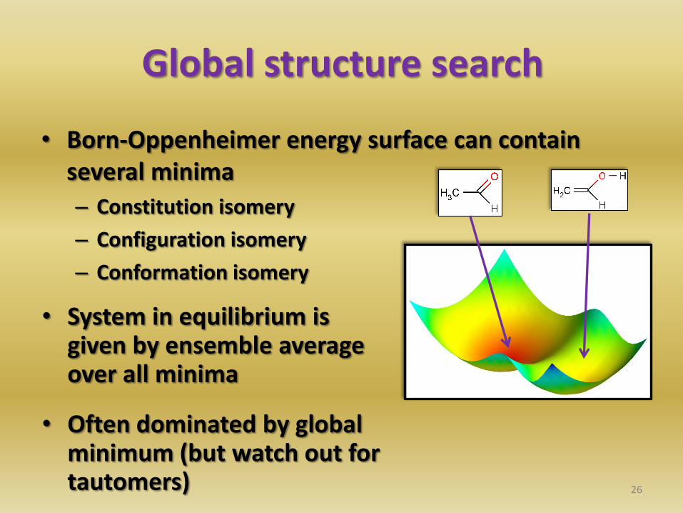
Global structure search
• Born-Oppenheimer energy surface can contain several minima
– Constitution isomery
– Configuration isomery
– Conformation isomery
26
• System in equilibrium is given by ensemble average over all minima
• Often dominated by global minimum (but watch out for tautomers)

Global structure search
• Methods to find the global minimum:
• Stochastical or Monte-Carlo
• Molecular dynamics: Simulated annealing [1,2]
• Genetic algorithm [3]
• Diffusion methods [4]
• Experimental structure determination
27
[1]: S. Kirkpatrick, et al., Science, (1983), 671 [2]: S.R. Wilson and W. Cui, Biopolymers (1990), 225 [3]: R.S. Judson, Rev. Comput Chem., (1997), 1 [4] J. Konstrowicki, H. A. Scheraga, J Phys. Chem. (1992), 7442
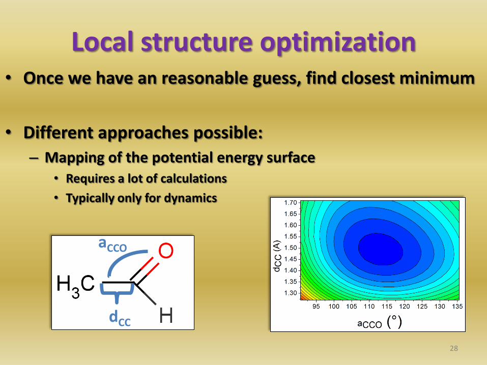
Local structure optimization • Once we have an reasonable guess, find closest minimum
• Different approaches possible:
– Mapping of the potential energy surface • Requires a lot of calculations
• Typically only for dynamics
28
dCC
aCCO
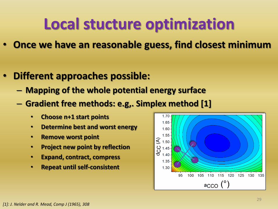
Local stucture optimization • Once we have an reasonable guess, find closest minimum
• Different approaches possible:
– Mapping of the whole potential energy surface
– Gradient free methods: e.g,. Simplex method [1]
29
• Choose n+1 start points
• Determine best and worst energy
• Remove worst point
• Project new point by reflection
• Expand, contract, compress
• Repeat until self-consistent
[1]: J. Nelder and R. Mead, Comp J (1965), 308
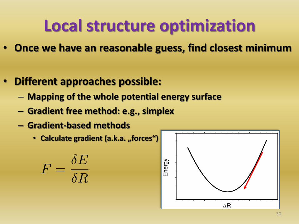
Local structure optimization • Once we have an reasonable guess, find closest minimum
• Different approaches possible:
– Mapping of the whole potential energy surface
– Gradient free method: e.g., simplex
– Gradient-based methods • Calculate gradient (a.k.a. „forces“)
30
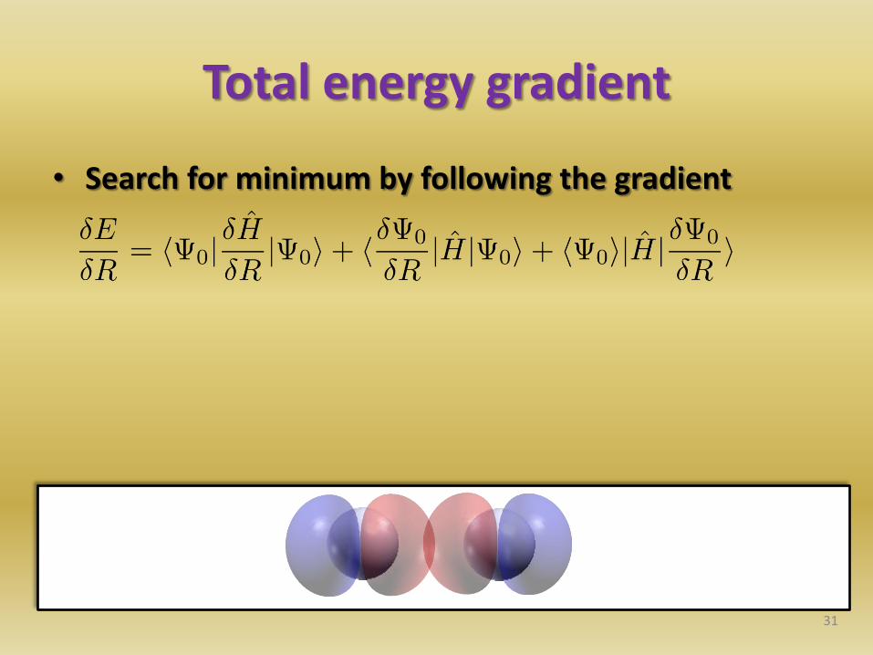
Total energy gradient
• Search for minimum by following the gradient
31
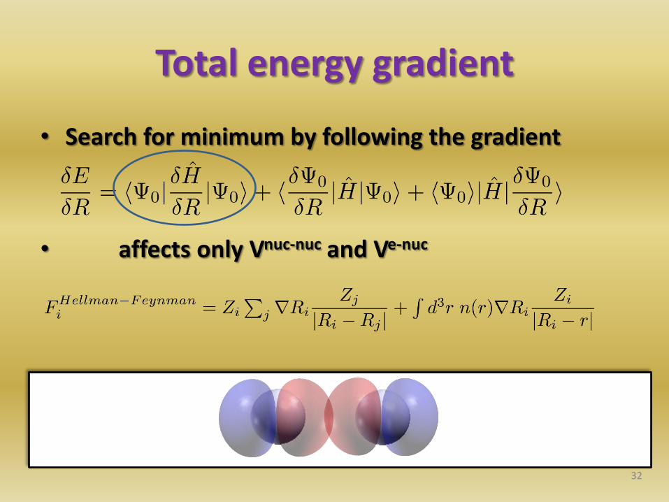
Total energy gradient
• Search for minimum by following the gradient
• affects only Vnuc-nuc and Ve-nuc
32
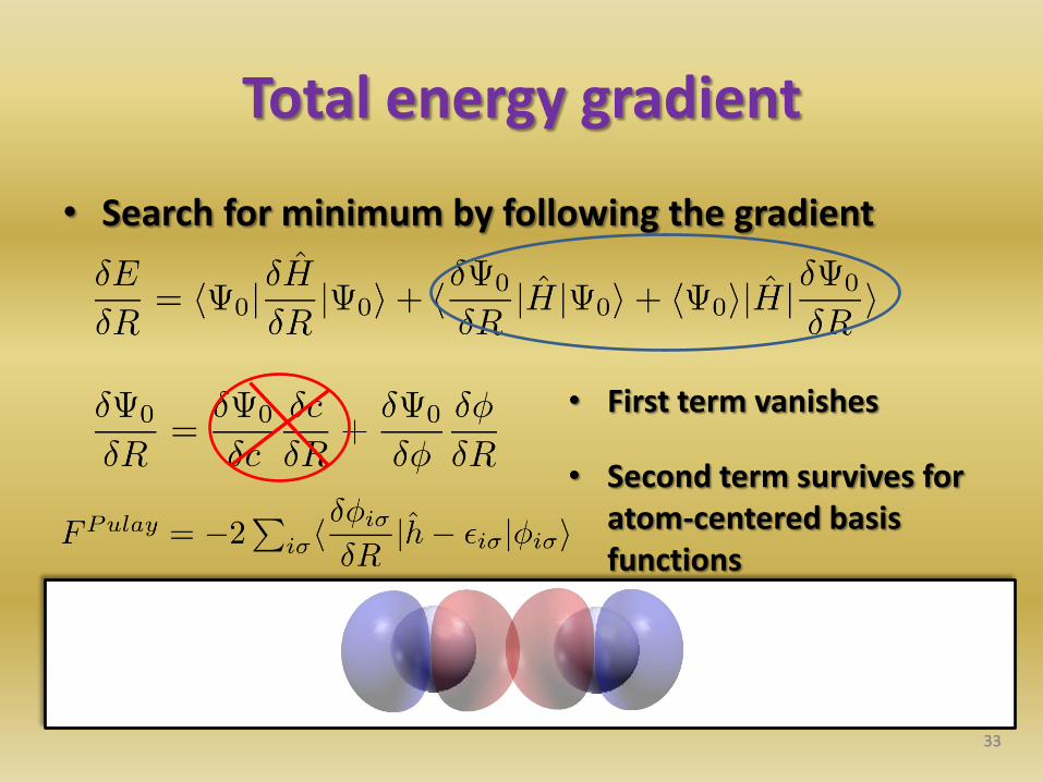
Total energy gradient
• Search for minimum by following the gradient
33
• First term vanishes
• Second term survives for atom-centered basis functions
33
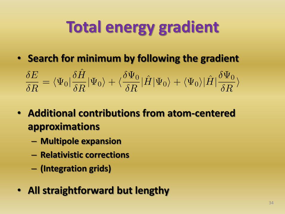
Total energy gradient
• Search for minimum by following the gradient
• Additional contributions from atom-centered approximations
– Multipole expansion
– Relativistic corrections
– (Integration grids)
• All straightforward but lengthy
34
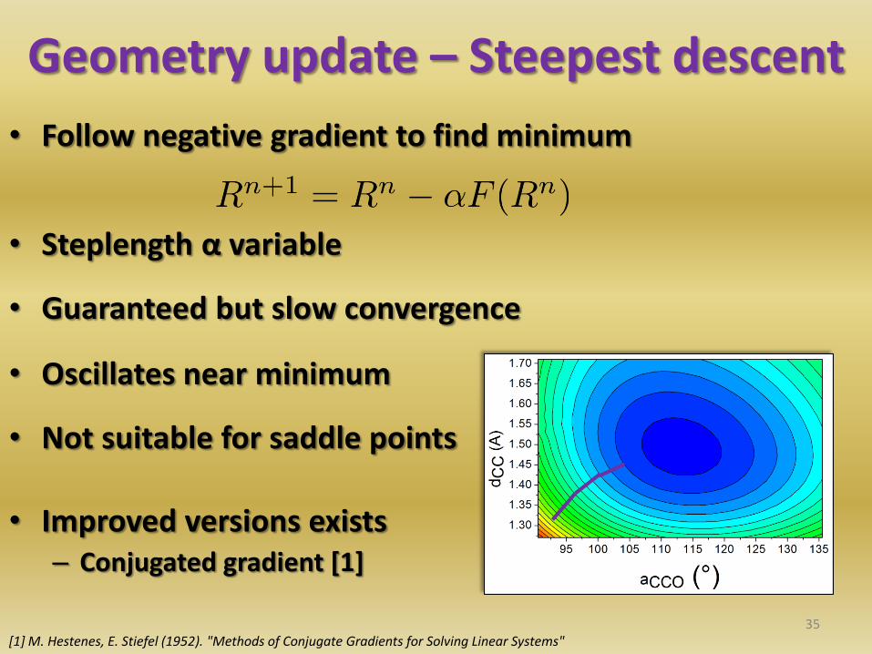
Geometry update – Steepest descent
• Follow negative gradient to find minimum
• Steplength α variable
• Guaranteed but slow convergence
• Oscillates near minimum
• Not suitable for saddle points
• Improved versions exists – Conjugated gradient [1]
35 [1] M. Hestenes, E. Stiefel (1952). "Methods of Conjugate Gradients for Solving Linear Systems"
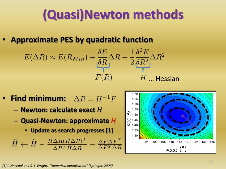
(Quasi)Newton methods
• Approximate PES by quadratic function
• Find minimum:
– Newton: calculate exact H
– Quasi-Newton: approximate H • Update as search progresses [1]
36
... Hessian
[1] J. Nocedal and S. J. Wright, “Numerical optimization” (Springer, 2006)
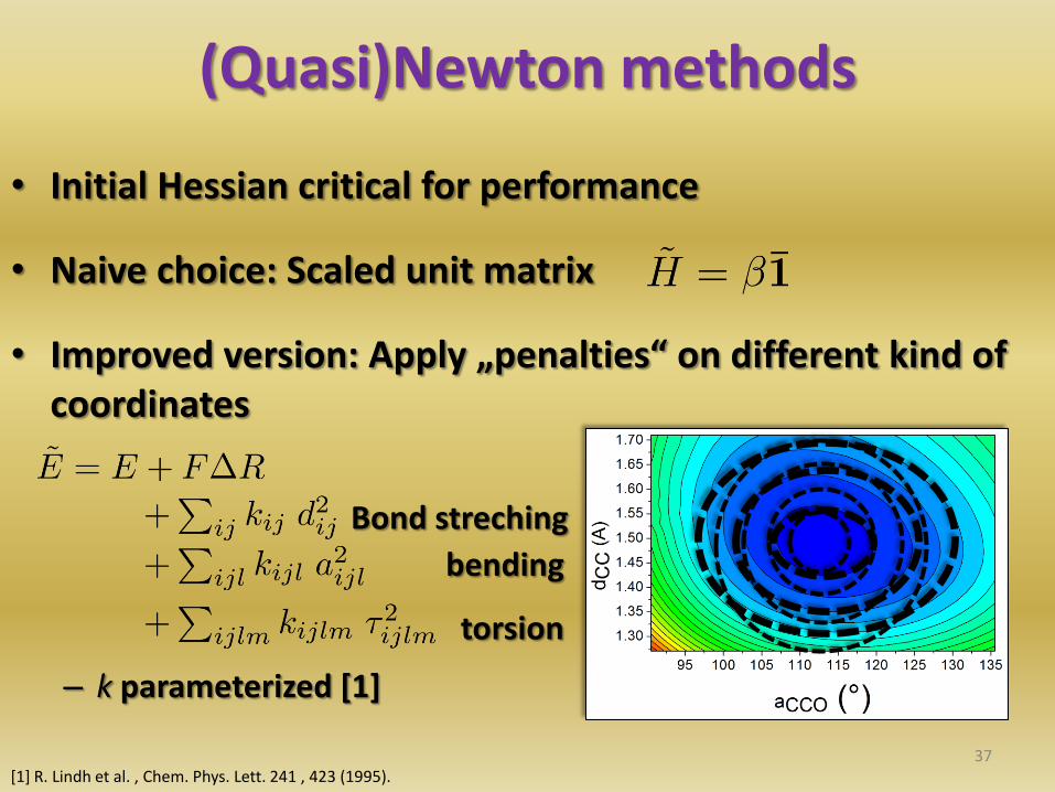
(Quasi)Newton methods
• Initial Hessian critical for performance
• Naive choice: Scaled unit matrix
• Improved version: Apply „penalties“ on different kind of coordinates
– k parameterized [1]
37 [1] R. Lindh et al. , Chem. Phys. Lett. 241 , 423 (1995).
Bond streching
bending
torsion
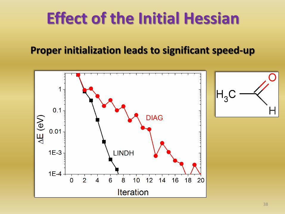
Effect of the Initial Hessian
38
Proper initialization leads to significant speed-up
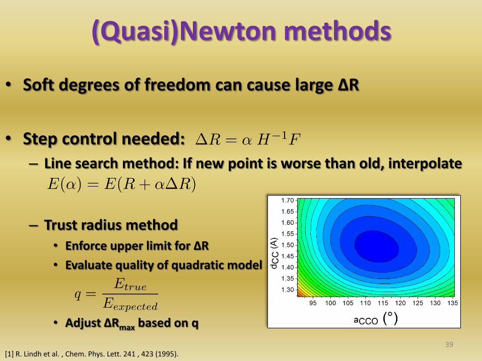
(Quasi)Newton methods
• Soft degrees of freedom can cause large ΔR
• Step control needed:
– Line search method: If new point is worse than old, interpolate
– Trust radius method • Enforce upper limit for ΔR
• Evaluate quality of quadratic model
• Adjust ΔRmax based on q
39
[1] R. Lindh et al. , Chem. Phys. Lett. 241 , 423 (1995).
Conclusions
• (Global optimization: PES feature-rich, methods to find global minima exist)
• Local geometry optimization: Follow gradient
– Hellman-Feynman from moving potentials
– Pulay from moving basis functions
– + additional terms
• Quasi-Newton method de-facto standard
– Require approximation and update of Hessian
– Step control by line search or trust radius method
40
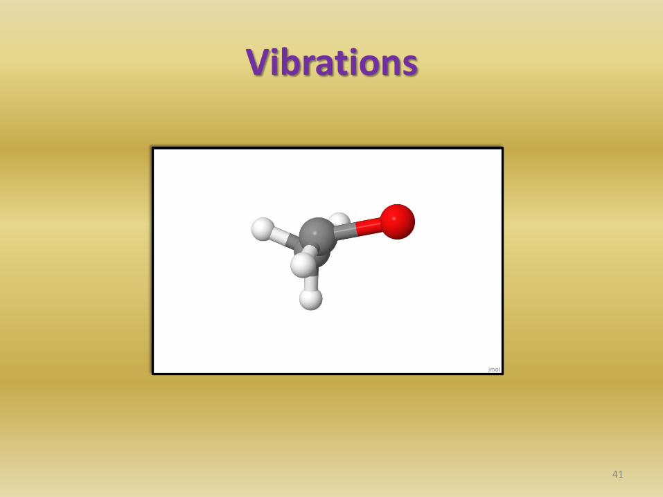
Vibrations
41
Vibrations
• Vibrations give important information about the system:
– Classification of stationary point (minimum / saddle point)
– If saddle-point: Provides search direction
– Thermodynamic data • Zero-point energy
• Partion sum
• Finite temperature effects
– Connection to experiment: • Infra-red intensities: derivative of dipole moment
• Raman intensities: derivative of polarizabilty
42
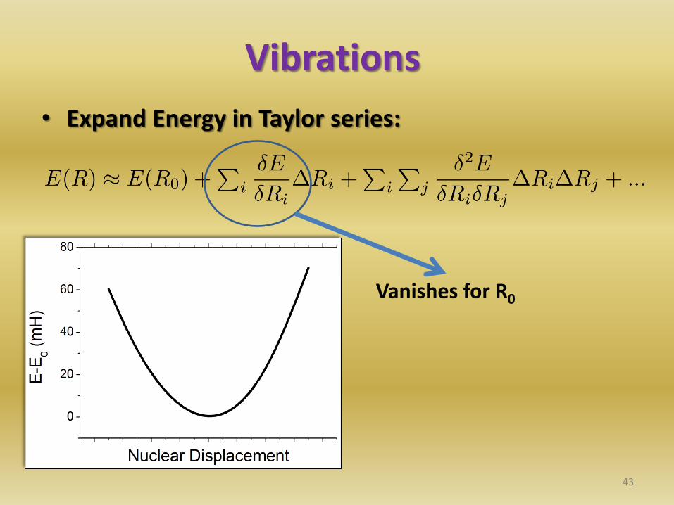
Vibrations
• Expand Energy in Taylor series:
43
Vanishes for R0
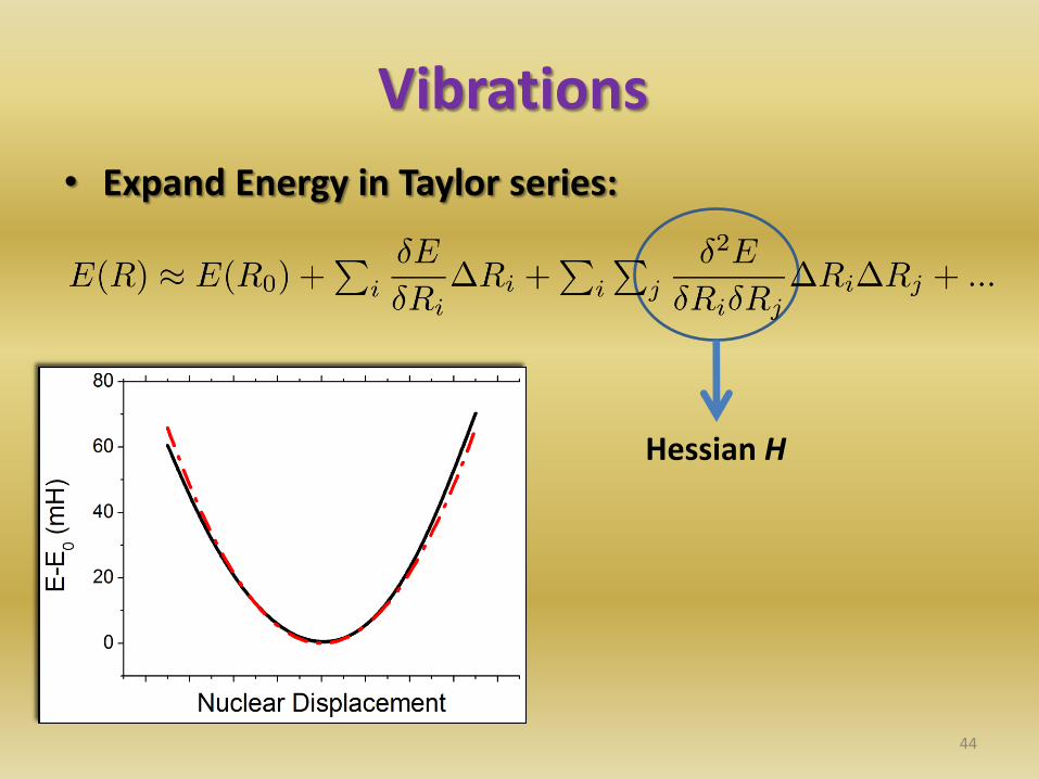
Vibrations
• Expand Energy in Taylor series:
44
Hessian H
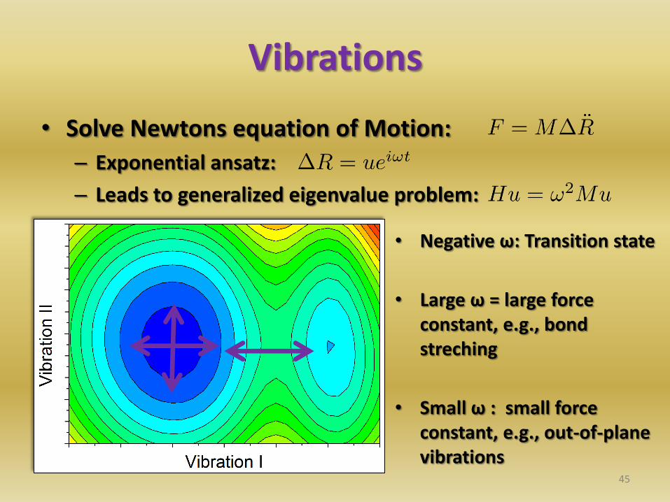
Vibrations
• Solve Newtons equation of Motion:
– Exponential ansatz:
– Leads to generalized eigenvalue problem:
45
• Negative ω: Transition state
• Large ω = large force constant, e.g., bond streching
• Small ω : small force constant, e.g., out-of-plane vibrations
Vibrations
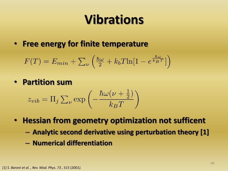
• Free energy for finite temperature
• Partition sum
• Hessian from geometry optimization not sufficent
– Analytic second derivative using perturbation theory [1]
– Numerical differentiation
46
[1] S. Baroni et al. , Rev. Mod. Phys. 73 , 515 (2001).
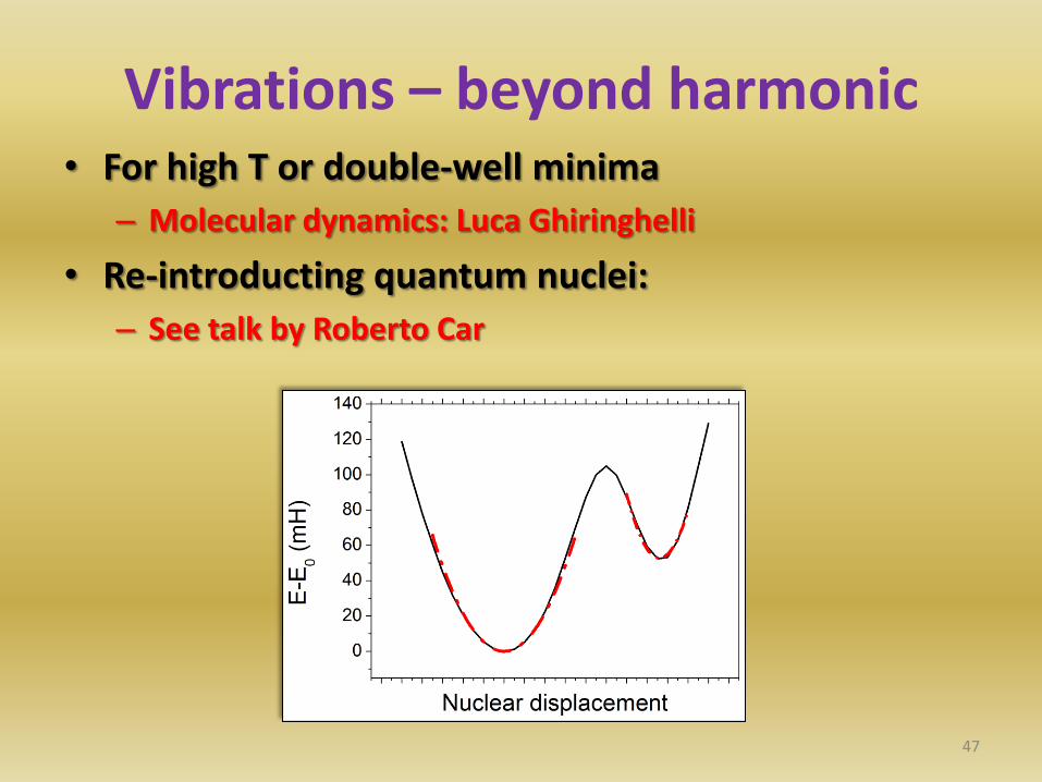
Vibrations – beyond harmonic • For high T or double-well minima
– Molecular dynamics: Luca Ghiringhelli
• Re-introducting quantum nuclei:
– See talk by Roberto Car
47
Conclusions
• Often calculated in harmonic approximation
• Yield information about stability of geometry
• Required for temperature effects
• Anharmonic effects via molecular dynamics
48
Visualization
49
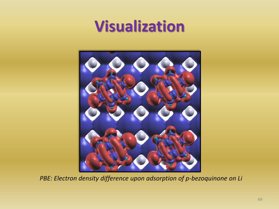
PBE: Electron density difference upon adsorption of p-bezoquinone on Li

Visualization
• Nuclear coordinates
• Electron distribution
• What else can we learn?
• How can we visualize results that are not just „numbers“
50
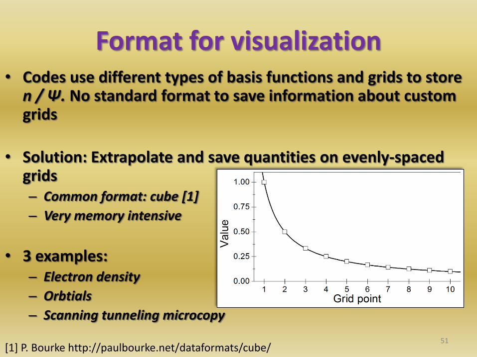
• Codes use different types of basis functions and grids to store n / Ψ. No standard format to save information about custom grids
• Solution: Extrapolate and save quantities on evenly-spaced grids – Common format: cube [1]
– Very memory intensive
• 3 examples: – Electron density
– Orbtials
– Scanning tunneling microcopy
Format for visualization
51 [1] P. Bourke http://paulbourke.net/dataformats/cube/
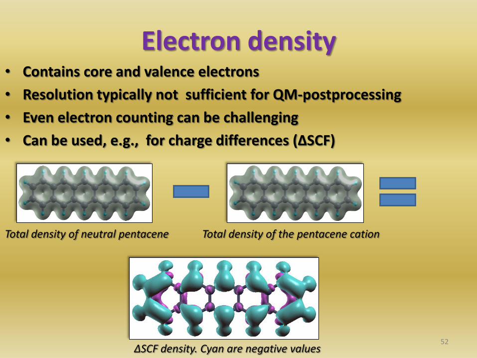
Electron density • Contains core and valence electrons
• Resolution typically not sufficient for QM-postprocessing
• Even electron counting can be challenging
• Can be used, e.g., for charge differences (ΔSCF)
52
Total density of neutral pentacene Total density of the pentacene cation
ΔSCF density. Cyan are negative values
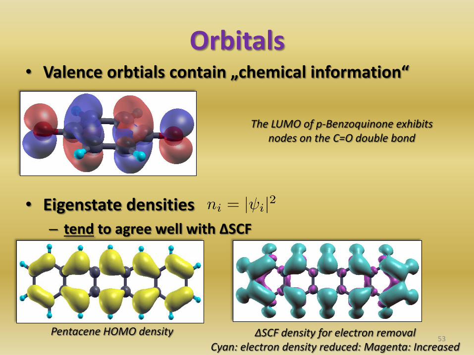
Orbitals • Valence orbtials contain „chemical information“
• Eigenstate densities
– tend to agree well with ΔSCF
53
ΔSCF density for electron removal Cyan: electron density reduced: Magenta: Increased
The LUMO of p-Benzoquinone exhibits nodes on the C=O double bond
Pentacene HOMO density
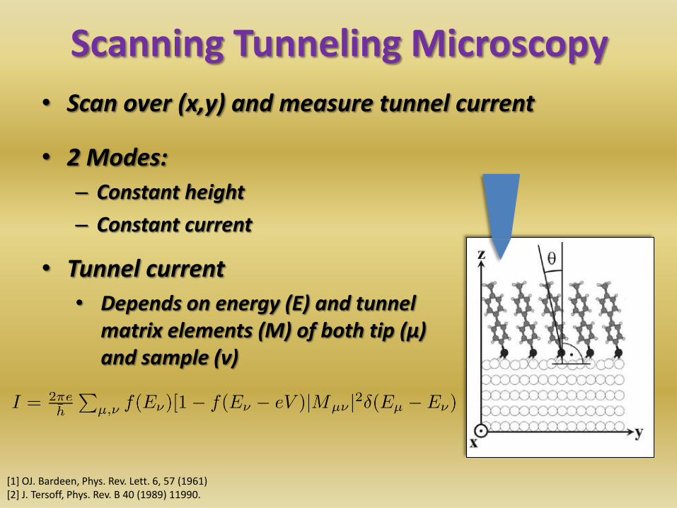
Scanning Tunneling Microscopy
[1] OJ. Bardeen, Phys. Rev. Lett. 6, 57 (1961) [2] J. Tersoff, Phys. Rev. B 40 (1989) 11990.
• Scan over (x,y) and measure tunnel current
• 2 Modes:
– Constant height
– Constant current
• Tunnel current
• Depends on energy (E) and tunnel matrix elements (M) of both tip (µ) and sample (ν)
Scanning Tunneling Microscopy
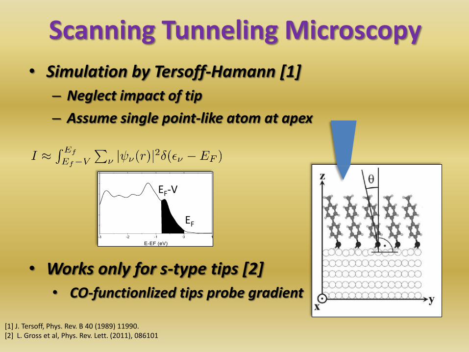
• Simulation by Tersoff-Hamann [1]
– Neglect impact of tip
– Assume single point-like atom at apex
• Works only for s-type tips [2]
• CO-functionlized tips probe gradient
[1] J. Tersoff, Phys. Rev. B 40 (1989) 11990. [2] L. Gross et al, Phys. Rev. Lett. (2011), 086101
EF
EF-V
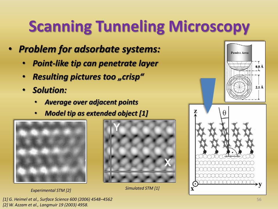
Scanning Tunneling Microscopy • Problem for adsorbate systems:
• Point-like tip can penetrate layer
• Resulting pictures too „crisp“
• Solution: • Average over adjacent points
• Model tip as extended object [1]
56 [1] G. Heimel et al., Surface Science 600 (2006) 4548–4562 [2] W. Azzam et al., Langmuir 19 (2003) 4958.
Experimental STM [2] Simulated STM [1]
Conclusion
• Electronic Schrödinger equation
– Solved by direct minimization or self-consistent field method
– Initial guess requires some thought
– Mixer: Tradeoff between stability and time
– Convergence accelleration: Preconditioner, Broadening
• Structure optimization
– Evaluate energy gradients
– Contribution from Hellman-Feynman and Pulay forces
– Solution by (Quasi)Newton-Methods
57
Conclusion
• Vibrations
– Information about stability of geometry
– Characterization of thermodynamic properties
– Allow to account for temperature effects
• Visualization
– Fields saved on regular grid
– Helpful for direction connection with experiment, e.g.: • Scanning tunneling microscopy
58

Thank you for your attention
59