Electronic Supplemental Information

for

Towards a unified understanding of the copper sites in particulate methane

monooxygenase: An X-ray absorption spectroscopic investigation

George E. Cutsail III,a,b* Matthew O. Ross,c,d Amy C. Rosenzweig,c Serena DeBeera*

a) Max Planck Institute for Chemical Energy Conversion, Stiftstrasse 34-36, D-45470

Mülheim an der Ruhr, Germany

b) University of Duisburg-Essen, Universitätsstrasse 7, D-45151 Essen, Germany

c) Departments of Molecular Biosciences and Chemistry, Northwestern University, Evanston

60208 IL, United States

d) Present address: Department of Chemistry, University of Chicago, Chicago, IL 60637,

United States

*Correspondence to: george.cutsail@cec.mpg.de, serena.debeer@cec.mpg.de

Electronic Supplementary Material (ESI) for Chemical Science.This journal is © The Royal Society of Chemistry 2021

1

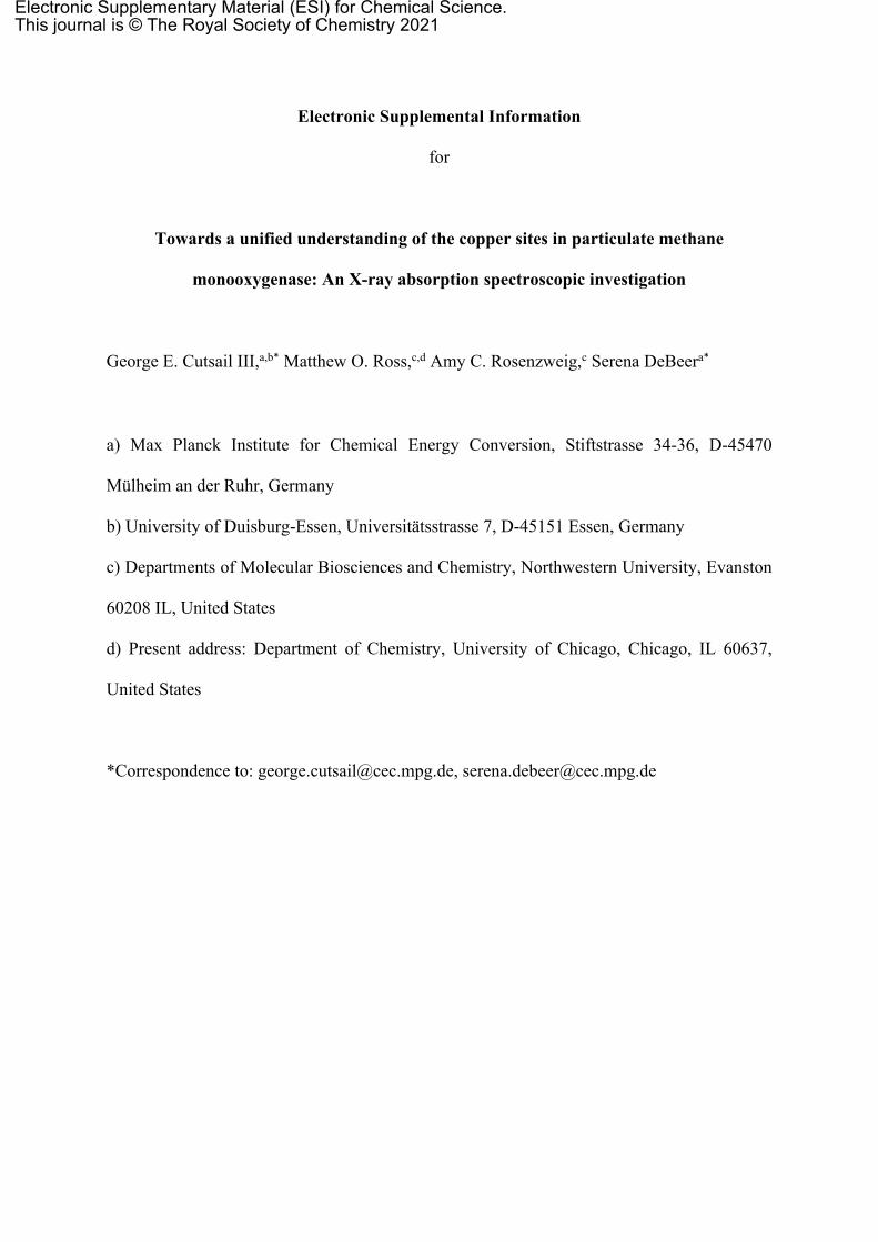
Figure S1. CW X-band EPR spectra of Bath-pMMO XAS samples Bath-pMMO-2021 (high

conc.) and Bath-pMMO-2021 (low conc). Brackets denote the CuB and CuC g|| and A|| values

measured previously1 (CuB g|| = 2.242, A|| = 182 G; CuC g|| = 2.30, A|| = 137 G). Heights

normalized to unity for ease of comparison. Collection conditions were as follows: 9.373-9.375

GHz microwave frequency, 320 ms time constant, 12.5 G modulation amplitude, 5 scans,

temperature 20 K.

2

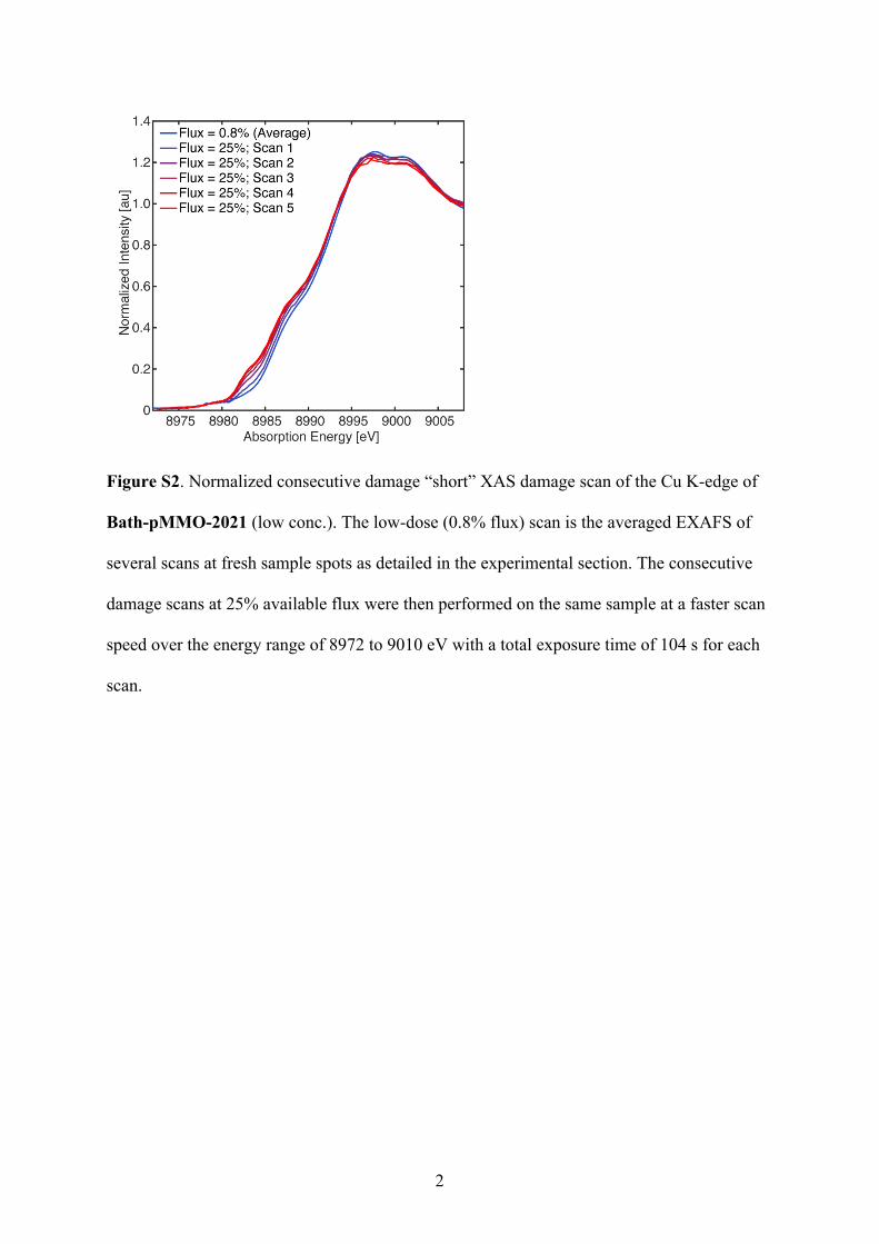
Figure S2. Normalized consecutive damage “short” XAS damage scan of the Cu K-edge of

Bath-pMMO-2021 (low conc.). The low-dose (0.8% flux) scan is the averaged EXAFS of

several scans at fresh sample spots as detailed in the experimental section. The consecutive

damage scans at 25% available flux were then performed on the same sample at a faster scan

speed over the energy range of 8972 to 9010 eV with a total exposure time of 104 s for each

scan.

3

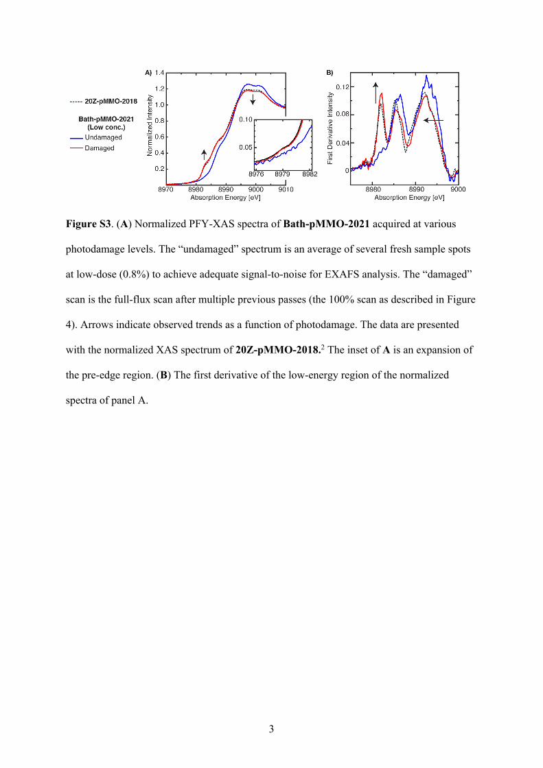
Figure S3. (A) Normalized PFY-XAS spectra of Bath-pMMO-2021 acquired at various

photodamage levels. The “undamaged” spectrum is an average of several fresh sample spots

at low-dose (0.8%) to achieve adequate signal-to-noise for EXAFS analysis. The “damaged”

scan is the full-flux scan after multiple previous passes (the 100% scan as described in Figure

4). Arrows indicate observed trends as a function of photodamage. The data are presented

with the normalized XAS spectrum of 20Z-pMMO-2018.2 The inset of A is an expansion of

the pre-edge region. (B) The first derivative of the low-energy region of the normalized

spectra of panel A.

4

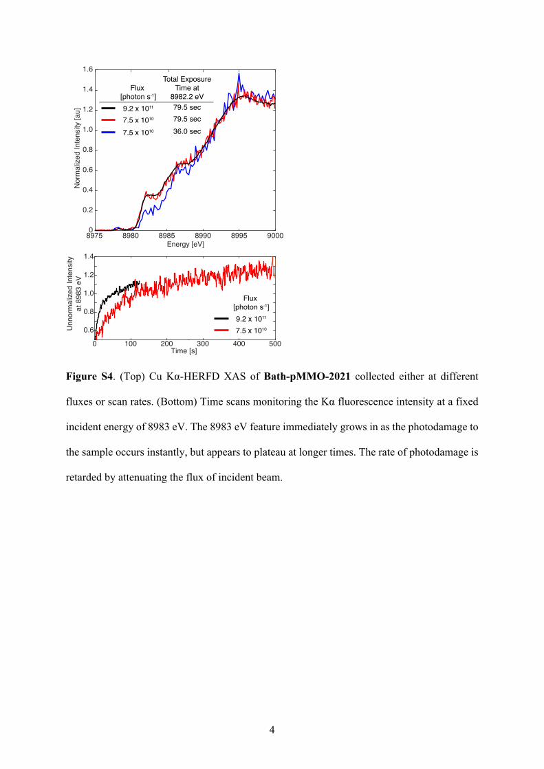
Figure S4. (Top) Cu Kα-HERFD XAS of Bath-pMMO-2021 collected either at different

fluxes or scan rates. (Bottom) Time scans monitoring the Kα fluorescence intensity at a fixed

incident energy of 8983 eV. The 8983 eV feature immediately grows in as the photodamage to

the sample occurs instantly, but appears to plateau at longer times. The rate of photodamage is

retarded by attenuating the flux of incident beam.

8975 8980 8985 8990 8995 9000Energy [eV]

0

0.2

0.4

0.6

0.8

1.0

1.2

1.4

1.6N

orm

aliz

ed In

tens

ity [a

u]Total Exposure

Time at8982.2 eV79.5 sec

36.0 sec

Flux [photon s-1]9.2 x 1011

7.5 x 1010

7.5 x 1010

79.5 sec

0 100 200 300 400 500Time [s]

0.6

0.8

1.0

1.2

1.4

Unn

orm

aliz

ed In

tens

ityat

898

3 eV

Flux [photon s-1]9.2 x 1011

7.5 x 1010

5

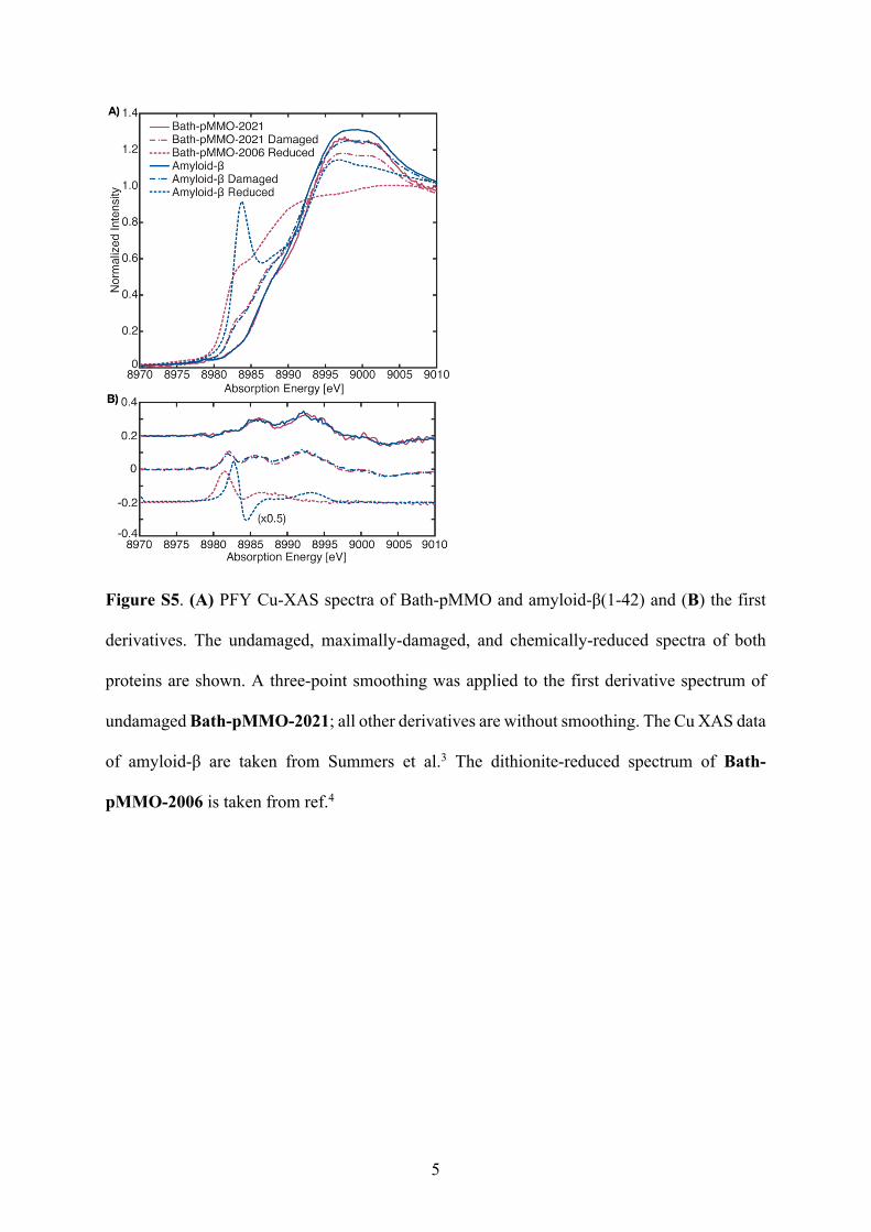
Figure S5. (A) PFY Cu-XAS spectra of Bath-pMMO and amyloid-β(1-42) and (B) the first

derivatives. The undamaged, maximally-damaged, and chemically-reduced spectra of both

proteins are shown. A three-point smoothing was applied to the first derivative spectrum of

undamaged Bath-pMMO-2021; all other derivatives are without smoothing. The Cu XAS data

of amyloid-β are taken from Summers et al.3 The dithionite-reduced spectrum of Bath-

pMMO-2006 is taken from ref.4

6

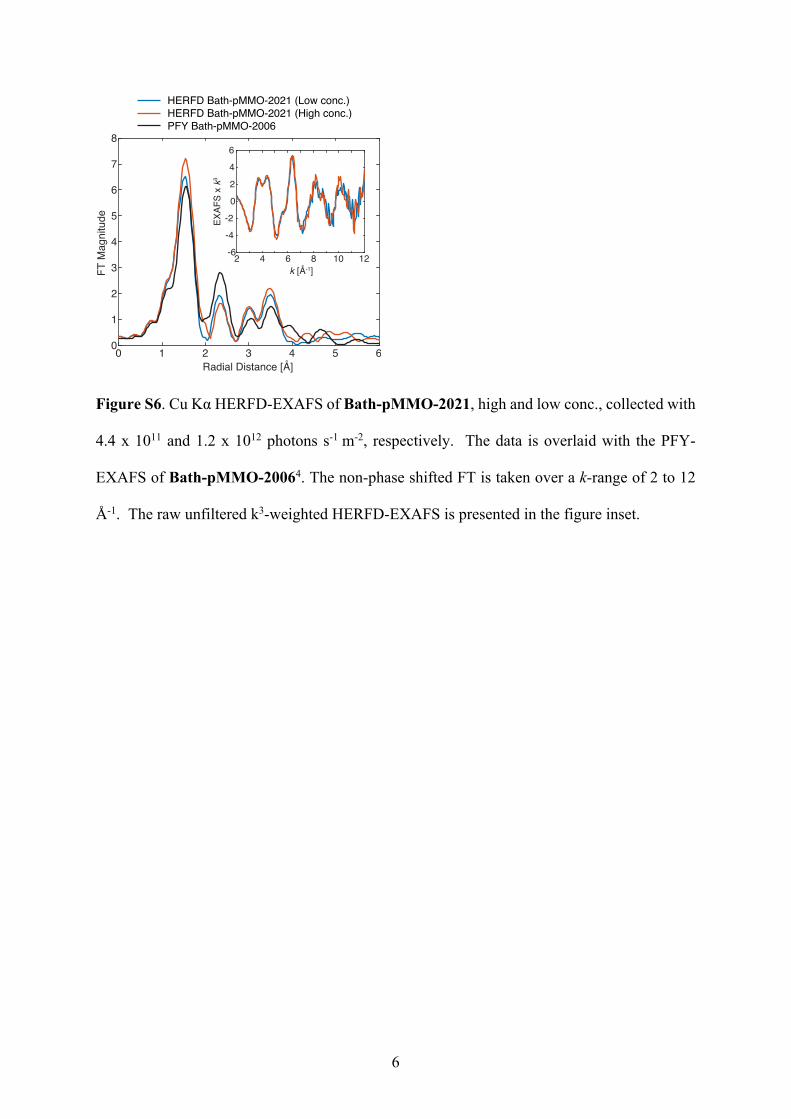
Figure S6. Cu Kα HERFD-EXAFS of Bath-pMMO-2021, high and low conc., collected with

4.4 x 1011 and 1.2 x 1012 photons s-1 m-2, respectively. The data is overlaid with the PFY-

EXAFS of Bath-pMMO-20064. The non-phase shifted FT is taken over a k-range of 2 to 12

Å-1. The raw unfiltered k3-weighted HERFD-EXAFS is presented in the figure inset.

0 1 2 3 4 5 6Radial Distance [Å]

0

1

2

3

4

5

6

7

8

FT M

agni

tude

HERFD Bath-pMMO-2021 (Low conc.)HERFD Bath-pMMO-2021 (High conc.)PFY Bath-pMMO-2006

2 4 6 8 10 12-6

-4

-2

0

2

4

6

k [Å-1]

EXAF

S x k3

7

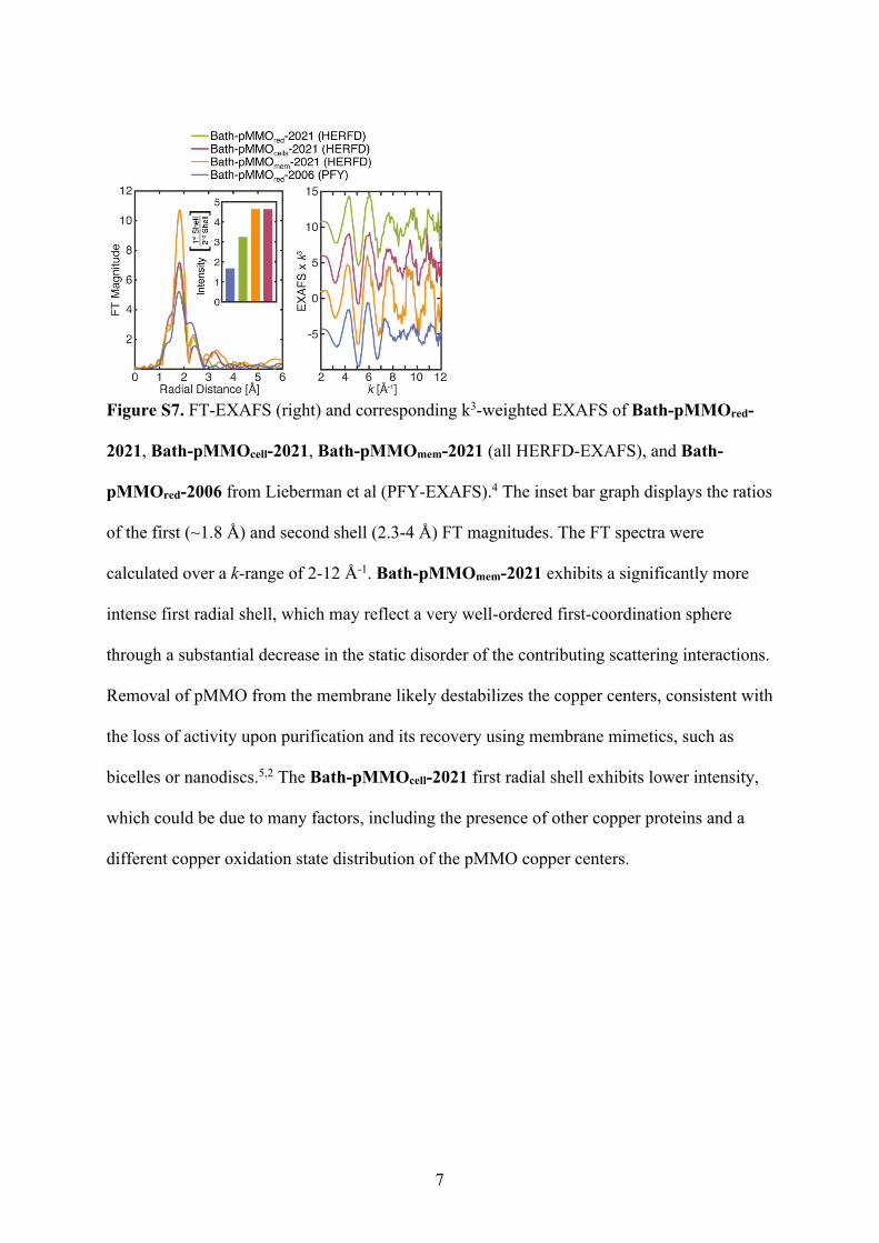
Figure S7. FT-EXAFS (right) and corresponding k3-weighted EXAFS of Bath-pMMOred-

2021, Bath-pMMOcell-2021, Bath-pMMOmem-2021 (all HERFD-EXAFS), and Bath-

pMMOred-2006 from Lieberman et al (PFY-EXAFS).4 The inset bar graph displays the ratios

of the first (~1.8 Å) and second shell (2.3-4 Å) FT magnitudes. The FT spectra were

calculated over a k-range of 2-12 Å-1. Bath-pMMOmem-2021 exhibits a significantly more

intense first radial shell, which may reflect a very well-ordered first-coordination sphere

through a substantial decrease in the static disorder of the contributing scattering interactions.

Removal of pMMO from the membrane likely destabilizes the copper centers, consistent with

the loss of activity upon purification and its recovery using membrane mimetics, such as

bicelles or nanodiscs.5,2 The Bath-pMMOcell-2021 first radial shell exhibits lower intensity,

which could be due to many factors, including the presence of other copper proteins and a

different copper oxidation state distribution of the pMMO copper centers.

8

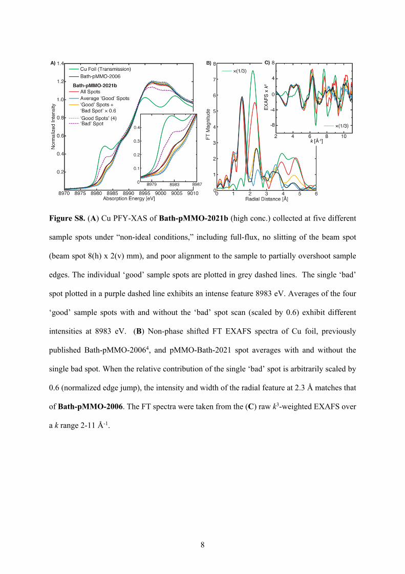
Figure S8. (A) Cu PFY-XAS of Bath-pMMO-2021b (high conc.) collected at five different

sample spots under “non-ideal conditions,” including full-flux, no slitting of the beam spot

(beam spot 8(h) x 2(v) mm), and poor alignment to the sample to partially overshoot sample

edges. The individual ‘good’ sample spots are plotted in grey dashed lines. The single ‘bad’

spot plotted in a purple dashed line exhibits an intense feature 8983 eV. Averages of the four

‘good’ sample spots with and without the ‘bad’ spot scan (scaled by 0.6) exhibit different

intensities at 8983 eV. (B) Non-phase shifted FT EXAFS spectra of Cu foil, previously

published Bath-pMMO-20064, and pMMO-Bath-2021 spot averages with and without the

single bad spot. When the relative contribution of the single ‘bad’ spot is arbitrarily scaled by

0.6 (normalized edge jump), the intensity and width of the radial feature at 2.3 Å matches that

of Bath-pMMO-2006. The FT spectra were taken from the (C) raw k3-weighted EXAFS over

a k range 2-11 Å-1.

9

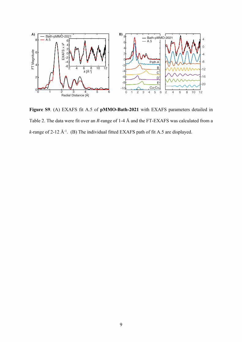
Figure S9. (A) EXAFS fit A.5 of pMMO-Bath-2021 with EXAFS parameters detailed in

Table 2. The data were fit over an R-range of 1-4 Å and the FT-EXAFS was calculated from a

k-range of 2-12 Å-1. (B) The individual fitted EXAFS path of fit A.5 are displayed.

10

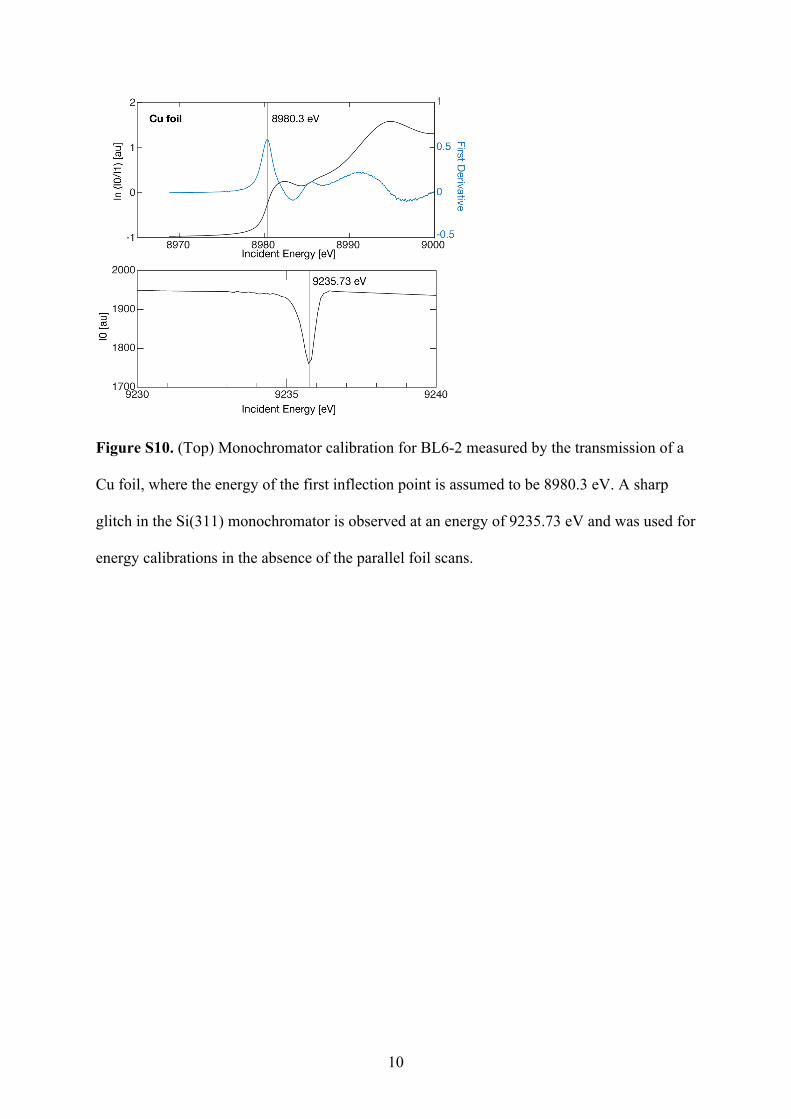
Figure S10. (Top) Monochromator calibration for BL6-2 measured by the transmission of a

Cu foil, where the energy of the first inflection point is assumed to be 8980.3 eV. A sharp

glitch in the Si(311) monochromator is observed at an energy of 9235.73 eV and was used for

energy calibrations in the absence of the parallel foil scans.

11

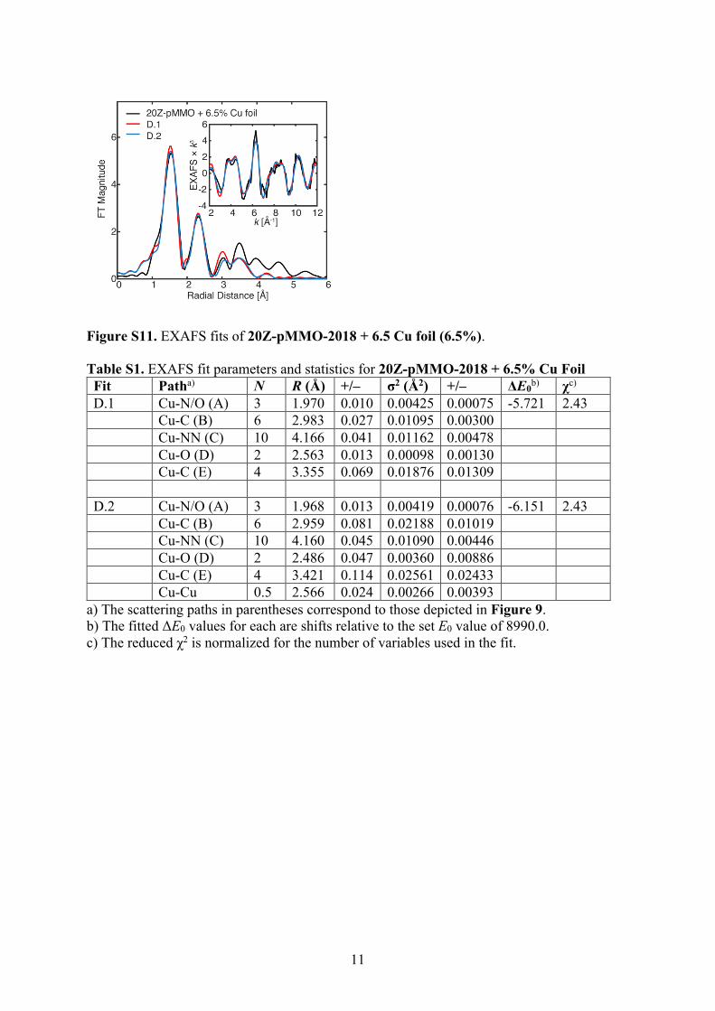
Figure S11. EXAFS fits of 20Z-pMMO-2018 + 6.5 Cu foil (6.5%).

Table S1. EXAFS fit parameters and statistics for 20Z-pMMO-2018 + 6.5% Cu Foil Fit Patha) N R (Å) +/– σ2 (Å2) +/– ΔE0b) χc) D.1 Cu-N/O (A) 3 1.970 0.010 0.00425 0.00075 -5.721 2.43 Cu-C (B) 6 2.983 0.027 0.01095 0.00300 Cu-NN (C) 10 4.166 0.041 0.01162 0.00478 Cu-O (D) 2 2.563 0.013 0.00098 0.00130 Cu-C (E) 4 3.355 0.069 0.01876 0.01309 D.2 Cu-N/O (A) 3 1.968 0.013 0.00419 0.00076 -6.151 2.43 Cu-C (B) 6 2.959 0.081 0.02188 0.01019 Cu-NN (C) 10 4.160 0.045 0.01090 0.00446 Cu-O (D) 2 2.486 0.047 0.00360 0.00886 Cu-C (E) 4 3.421 0.114 0.02561 0.02433 Cu-Cu 0.5 2.566 0.024 0.00266 0.00393

a) The scattering paths in parentheses correspond to those depicted in Figure 9. b) The fitted ΔE0 values for each are shifts relative to the set E0 value of 8990.0. c) The reduced χ2 is normalized for the number of variables used in the fit.

12

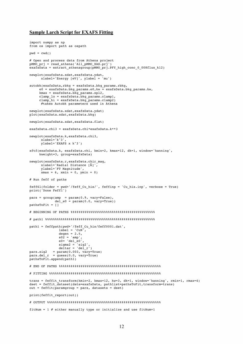
Sample Larch Script for EXAFS Fitting

import numpy as np from os import path as ospath pwd = cwd() # Open and process data from Athena project pMMO_prj = read_athena('All_pMMO_XAS.prj') exafsData = extract_athenagroup(pMMO_prj.PFY_high_conc_0_008flux_k12) newplot(exafsData.xdat,exafsData.ydat, xlabel='Energy [eV]', ylabel = 'mu') autobk(exafsData,rbkg = exafsData.bkg_params.rbkg, e0 = exafsData.bkg_params.e0,kw = exafsData.bkg_params.kw, kmax = exafsData.bkg_params.spl2, clamp_lo = exafsData.bkg_params.clamp1, clamp_hi = exafsData.bkg_params.clamp2)

#takes Autobk parameters used in Athena newplot(exafsData.xdat,exafsData.ydat) plot(exafsData.xdat,exafsData.bkg) newplot(exafsData.xdat,exafsData.flat) exafsData.chi3 = exafsData.chi*exafsData.k**3 newplot(exafsData.k,exafsData.chi3, xlabel='k^3', ylabel='EXAFS x k^3') xftf(exafsData.k, exafsData.chi, kmin=2, kmax=12, dk=1, window='hanning', kweight=3, group=exafsData) newplot(exafsData.r,exafsData.chir_mag, xlabel='Radial Distance [Å]', ylabel='FT Magnitude', xmax = 6, xmin = 0, ymin = 0) # Run feff of paths feff6l(folder = pwd+'/feff_Cu_his/', feffinp = 'Cu_his.inp', verbose = True) print('Done Feff1') pars = group(amp = param(0.9, vary=False), del_e0 = param(0.0, vary=True)) pathsToFit = [] # BEGINNING OF PATHS %%%%%%%%%%%%%%%%%%%%%%%%%%%%%%%%%%%%%%%%%%% # path1 %%%%%%%%%%%%%%%%%%%%%%%%%%%%%%%%%%%%%%%%%%%%%%%%%%%%%%%% path1 = feffpath(pwd+'/feff_Cu_his/feff0001.dat', label = 'CuN', degen = 2.5, s02 = 'amp', e0= 'del_e0', sigma2 = 'sig2', deltar = 'del_r') pars.sig2 = param(0.003, vary=True) pars.del_r = guess(0.0, vary=True) pathsToFit.append(path1) # END OF PATHS %%%%%%%%%%%%%%%%%%%%%%%%%%%%%%%%%%%%%%%%%%%%%%%%%%%% # FITTING %%%%%%%%%%%%%%%%%%%%%%%%%%%%%%%%%%%%%%%%%%%%%%%%%%%%%%%%% trans = feffit_transform(kmin=2, kmax=12, kw=3, dk=1, window='hanning', rmin=1, rmax=4) dset = feffit_dataset(data=exafsData, pathlist=pathsToFit,transform=trans) out = feffit(paramgroup = pars, datasets = dset) print(feffit_report(out)) # OUTPUT %%%%%%%%%%%%%%%%%%%%%%%%%%%%%%%%%%%%%%%%%%%%%%%%%%%%%%%%%% fitNum = 1 # either manually type or initialize and use fitNum+1

13

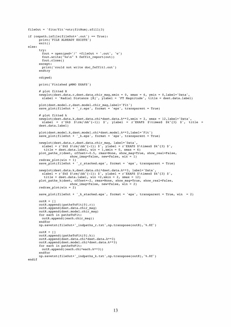
fileOut = 'fits/fit'+str(fitNum).zfill(3) if (ospath.isfile(fileOut+'.out') == True): print('FILE ALREADY EXISTS') exit() else: try: fout = open(pwd+'/' +fileOut + '.out', 'w') fout.write("%s\n" % feffit_report(out)) fout.close() except: print('could not write doc_feffit1.out') endtry cd(pwd) print('Finished pMMO EXAFS') # plot fitted R newplot(dset.data.r,dset.data.chir_mag,xmin = 0, xmax = 6, ymin = 0,label='Data', xlabel = 'Radial Distance [Å]', ylabel = 'FT Magnitude', title = dset.data.label) plot(dset.model.r,dset.model.chir_mag,label='Fit') save_plot(fileOut + '_r.eps', format = 'eps', transparent = True) # plot fitted k newplot(dset.data.k,dset.data.chi*dset.data.k**3,xmin = 2, xmax = 12,label='Data', xlabel = r'$k$ $\rm(\AA^{-1}) $', ylabel = r'EXAFS $\times$ $k^{3} $', title =

dset.data.label) plot(dset.model.k,dset.model.chi*dset.model.k**3,label='Fit') save_plot(fileOut + '_k.eps', format = 'eps', transparent = True) newplot(dset.data.r,dset.data.chir_mag, label='Data', xlabel = r'$k$ $\rm(\AA^{-1}) $', ylabel = r'EXAFS $\times$ $k^{3} $', title = dset.data.label, win = 1,xmin = 0, xmax = 6) plot_paths_r(dset, offset=-0.5, rmax=None, show_mag=True, show_real=False, show_imag=False, new=False, win = 1) redraw_plot(win = 1) save_plot(fileOut + '_r_stacked.eps', format = 'eps', transparent = True) newplot(dset.data.k,dset.data.chi*dset.data.k**3, label='Data', xlabel = r'$k$ $\rm(\AA^{-1}) $', ylabel = r'EXAFS $\times$ $k^{3} $', title = dset.data.label, win =2,xmin = 2, xmax = 12) plot_paths_k(dset, offset=-2, rmax=None, show_mag=True, show_real=False, show_imag=False, new=False, win = 2) redraw_plot(win = 2) save_plot(fileOut + '_k_stacked.eps', format = 'eps', transparent = True, win = 2) outR = [] outR.append((pathsToFit[0].r)) outR.append(dset.data.chir_mag) outR.append(dset.model.chir_mag) for each in pathsToFit: outR.append((each.chir_mag)) endfor np.savetxt(fileOut+'_indpaths_r.txt',np.transpose(outR),'%.8f') outK = [] outK.append((pathsToFit[0].k)) outK.append(dset.data.chi*dset.data.k**3) outK.append(dset.model.chi*dset.data.k**3) for each in pathsToFit: outK.append((each.chi*each.k**3)) endfor np.savetxt(fileOut+'_indpaths_k.txt',np.transpose(outK),'%.8f') endif

14

References

1. M. O. Ross, F. MacMillan, J. Wang, A. Nisthal, T. J. Lawton, B. D. Olafson, S. L. Mayo, A. C. Rosenzweig and B. M. Hoffman, Science, 2019, 364, 566-570.

2. S. Y. Ro, M. O. Ross, Y. W. Deng, S. Batelu, T. J. Lawton, J. D. Hurley, T. L. Stemmler, B. M. Hoffman and A. C. Rosenzweig, J. Biol. Chem., 2018, 293, 10457-10465.

3. K. L. Summers, K. M. Schilling, G. Roseman, K. A. Markham, N. V. Dolgova, T. Kroll, D. Sokaras, G. L. Millhauser, I. J. Pickering and G. N. George, Inorg. Chem., 2019, 58, 6294-6311.

4. R. L. Lieberman, K. C. Kondapalli, D. B. Shrestha, A. S. Hakemian, S. M. Smith, J. Telser, J. Kuzelka, R. Gupta, A. S. Borovik, S. J. Lippard, B. M. Hoffman, A. C. Rosenzweig and T. L. Stemmler, Inorg. Chem., 2006, 45, 8372-8381.

5. S. Y. Ro, L. F. Schachner, C. W. Koo, R. Purohit, J. P. Remis, G. E. Kenney, B. W. Liauw, P. M. Thomas, S. M. Patrie, N. L. Kelleher and A. C. Rosenzweig, Nat. Commun., 2019, 10, 2675.