1

Electronics Simulation in thePhoton Transport Monte Carlo

• Preamp model

• Receiver/discriminator circuit

• CAFÉ driver circuit model

• Examples

• Summary

January 31, 2005 – last update: Jan 30

Matthew Jones/Riei Ishiziki

Purdue University

2

Preamp Model

• So far, the effect of the preamp has been ignored, although some degradation in rise-time was included. This was just a wild guess.

• Need a good preamp model to relate anode charge to output of ADC…

• Particularly important for large pulses.• Best studied using SPICE simulation of preamp

circuit.• Useful check of schematics for the NIM paper.

3

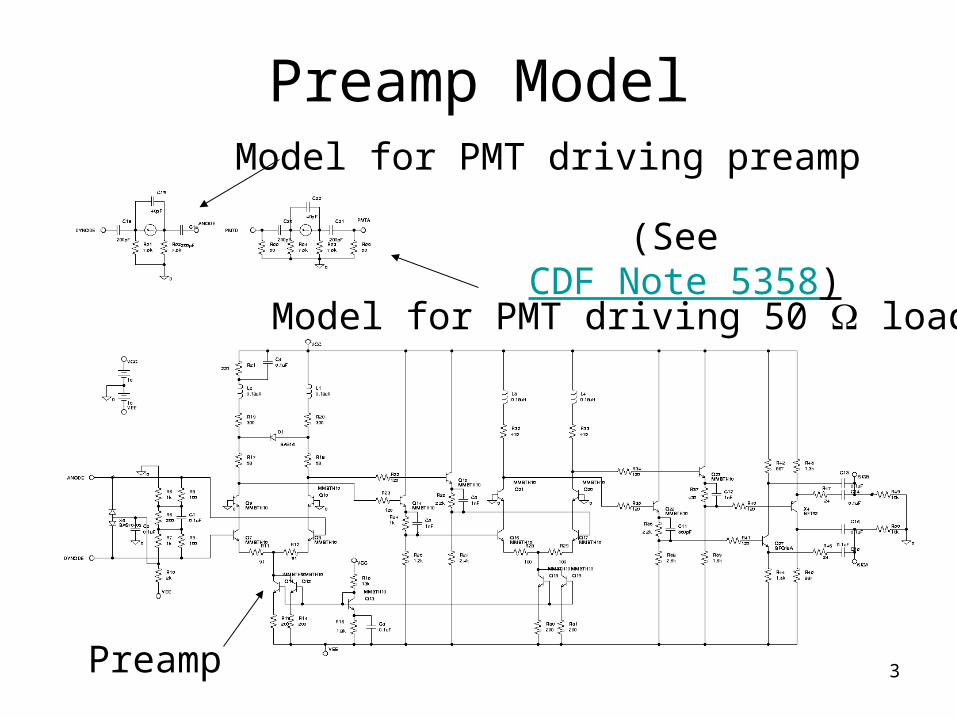
Preamp ModelModel for PMT driving preamp

Model for PMT driving 50 load

Preamp

(See CDF Note 5358)

4

Preamp Model

• Important to validate the simulation by comparing with real preamp.

• Input pulse:– Gaussian, 1.5ns width, typically 0.01 nC– 0.01 nC corresponds to 2080 p.e. when the

PMT gain is 3x104

• Allows comparison with preamp checkout measurements performed with charge injector.

5

Preamp Model

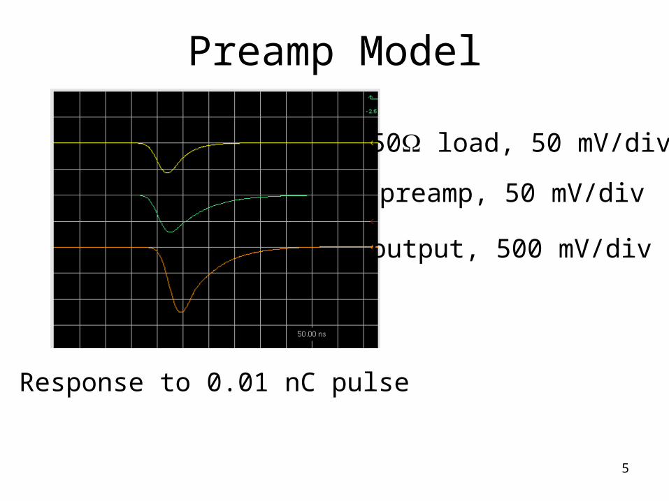
Response to 0.01 nC pulse

50 load, 50 mV/div

preamp, 50 mV/div

output, 500 mV/div

6

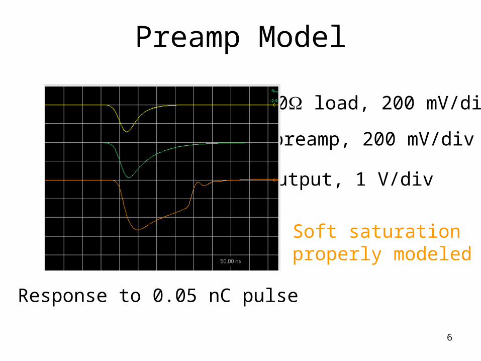
Preamp Model

Response to 0.05 nC pulse

50 load, 200 mV/div

preamp, 200 mV/div

output, 1 V/div

Soft saturationproperly modeled

7

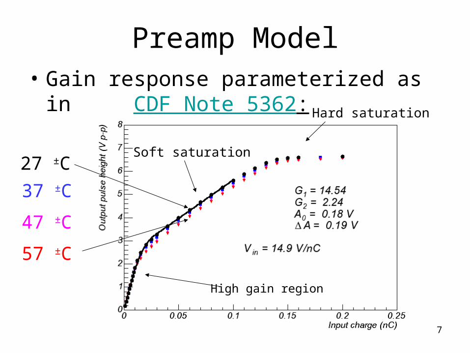
Preamp Model• Gain response parameterized as in

CDF Note 5362:

High gain region

Soft saturation

Hard saturation

27 ±C

37 ±C

47 ±C

57 ±C

8

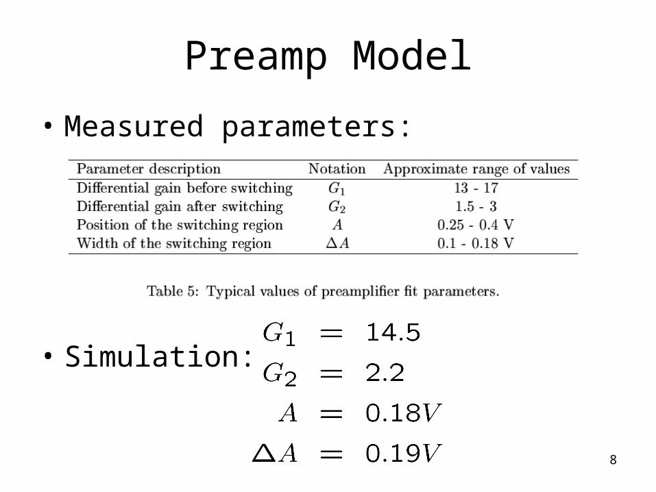
Preamp Model

• Measured parameters:

• Simulation:

9

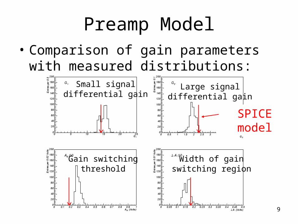
Preamp Model• Comparison of gain parameters with

measured distributions:Small signal

differential gainLarge signal

differential gain

Gain switchingthreshold

Width of gainswitching region

SPICE model

10

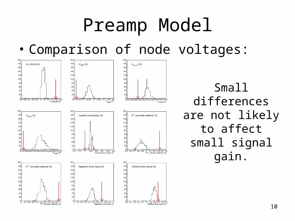
Preamp Model• Comparison of node voltages:

Small differences are not likely to

affect small signal gain.

11

Preamp Model• Probable unknowns:

– Supply voltages in the detector• Measure them next time the plugs are open

– Temperature in the detector– No simulation of parasitic capacitance– Parameters for gain switching diode model

• Qualitative behavior seems reasonable.• Small signal response agrees well with

measurements and should be adequately described.

12

Preamp Model

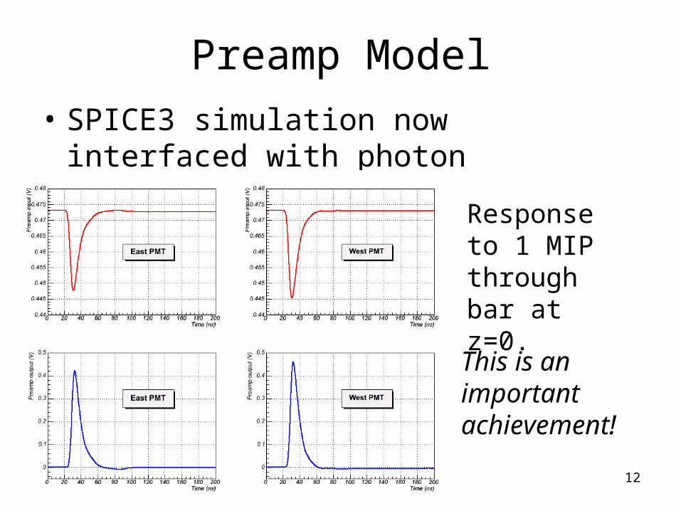
• SPICE3 simulation now interfaced with photon transport Monte Carlo:

Response to 1 MIP through bar at z=0.

This is an important achievement!

13

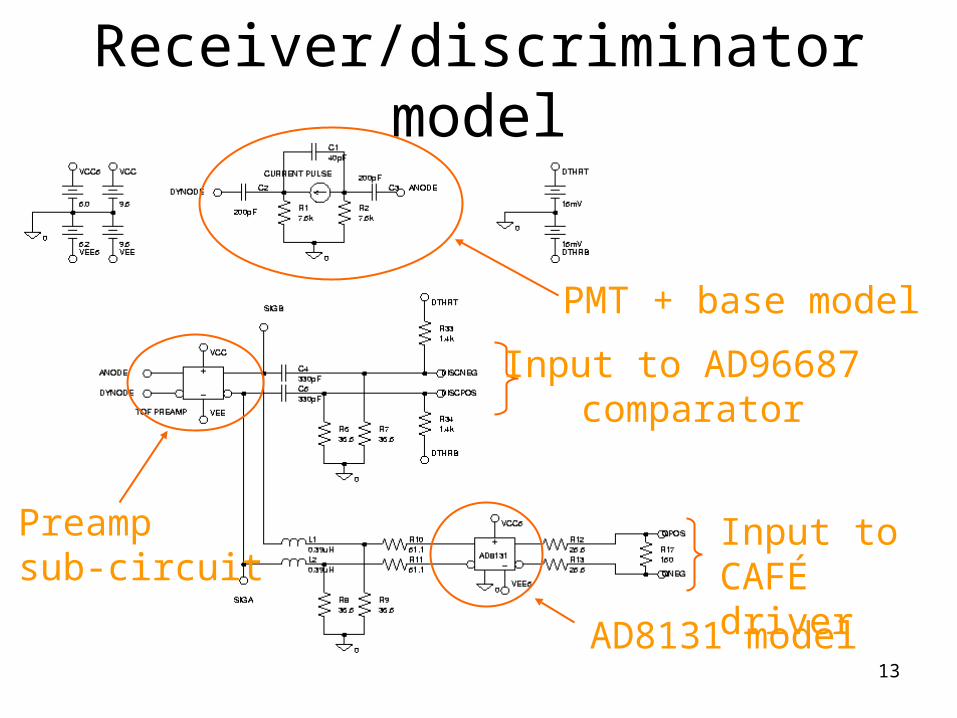
Receiver/discriminator model

Preampsub-circuit

Input to AD96687 comparator

AD8131 model

PMT + base model

Input to CAFÉ driver

14

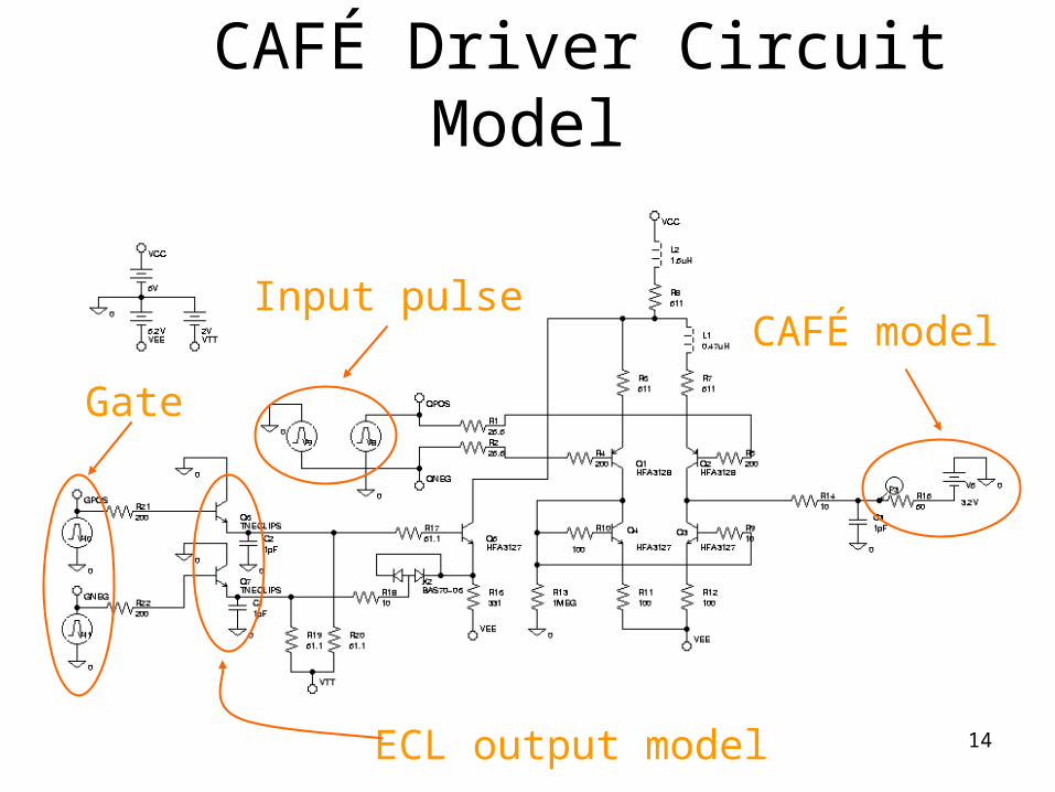
CAFÉ Driver Circuit Model

Input pulseCAFÉ model

ECL output model

Gate

15

TOAD Electronics

• Still should perform more validation:– Compare with production TOAD board node

voltages– Still not simulating signal cable (22 m

attenuation length) and RF transformer– Need to determine phase of CAFÉ clock– Include parasitic capacitances on TOAD and

connector inductances to CAFÉ card

16

Software Interface

• Interfaced with photon transport MC:– PMT class constructs SPICE3 model for current pulse

at the anode.– System call to invoke SPICE3 with circuit models– Output vectors read from binary file– Currently stored as non-persistent TGraph objects

• Simulation is fast (few seconds) compared with photon propagation

17

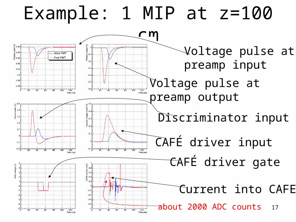
Example: 1 MIP at z=100 cmVoltage pulse atpreamp input

Voltage pulse atpreamp output

Discriminator input

CAFÉ driver input

CAFÉ driver gate

Current into CAFE

about 2000 ADC counts

18

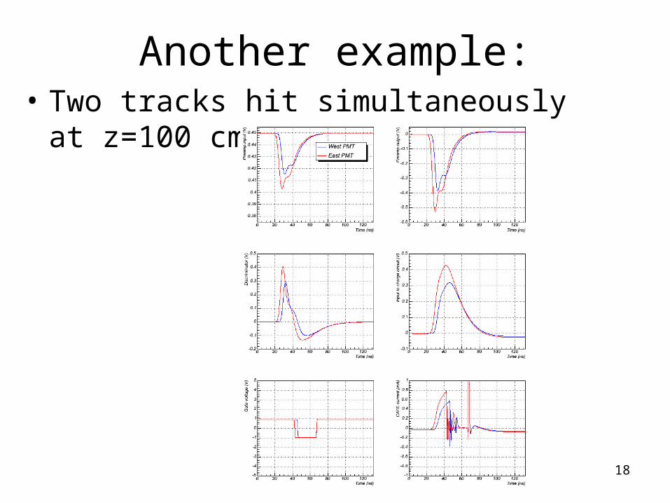
Another example:• Two tracks hit simultaneously at z=100 cm

and z=-50cm:

19

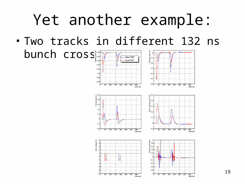
Yet another example:• Two tracks in different 132 ns bunch

crossings:

20

Electronics Simulation• It is now possible to study:

– Absolute scale of discriminator threshold– Functional form of time slewing correction– ADC bias due to multiple hits– Baseline shifts from hits in earlier bunch

crossings (luminosity dependence of ADC)– ADC response to monopoles, MIP’s, etc.

• Limiting factors will probably come from the PMT parameters (photocathode sensitivity, absolute gain) and scintillator.

21

Summary

• SPICE3 models:– Preamp: good shape now– Discriminator: should be okay

• Use simulation instead of parameterized model?• Need to check threshold circuit in more detail.

– CAFE driver: Predicted ADC counts have the right order of magnitude!

• Still need to work out the phase of the CAFÉ integration gate• Now we will have to subtract pedestals in the simulation

• Real limitation probably comes from things we can’t measure (PMT and scintillator properties).