Electronics Tutorial about AC Waveforms

AC Waveform Navigation

Tutorial: 1 of 12

--- Select a Tutorial Page ---

RESET

The AC Waveform

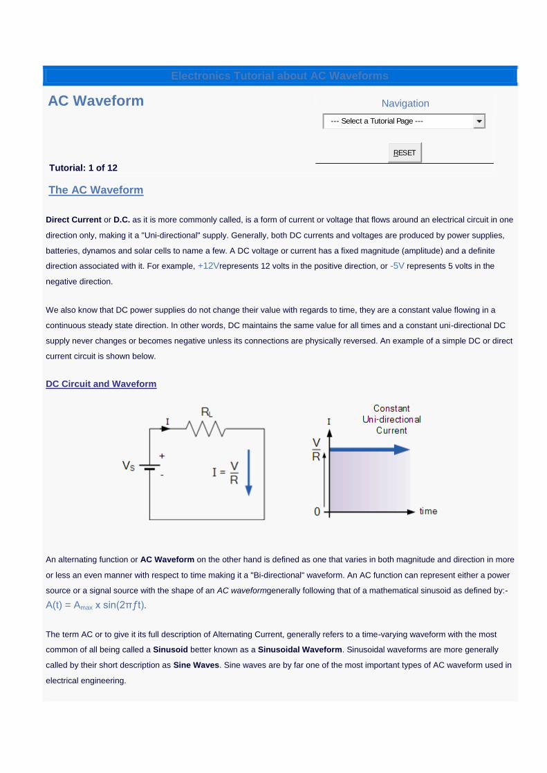
Direct Current or D.C. as it is more commonly called, is a form of current or voltage that flows around an electrical circuit in one

direction only, making it a "Uni-directional" supply. Generally, both DC currents and voltages are produced by power supplies,

batteries, dynamos and solar cells to name a few. A DC voltage or current has a fixed magnitude (amplitude) and a definite

direction associated with it. For example, +12Vrepresents 12 volts in the positive direction, or -5V represents 5 volts in the

negative direction.

We also know that DC power supplies do not change their value with regards to time, they are a constant value flowing in a

continuous steady state direction. In other words, DC maintains the same value for all times and a constant uni-directional DC

supply never changes or becomes negative unless its connections are physically reversed. An example of a simple DC or direct

current circuit is shown below.

DC Circuit and Waveform

An alternating function or AC Waveform on the other hand is defined as one that varies in both magnitude and direction in more

or less an even manner with respect to time making it a "Bi-directional" waveform. An AC function can represent either a power

source or a signal source with the shape of an AC waveformgenerally following that of a mathematical sinusoid as defined by:-

A(t) = Amax x sin(2πƒt).

The term AC or to give it its full description of Alternating Current, generally refers to a time-varying waveform with the most

common of all being called a Sinusoid better known as a Sinusoidal Waveform. Sinusoidal waveforms are more generally

called by their short description as Sine Waves. Sine waves are by far one of the most important types of AC waveform used in

electrical engineering.

The shape obtained by plotting the instantaneous ordinate values of either voltage or current against time is called an AC

Waveform. An AC waveform is constantly changing its polarity every half cycle alternating between a positive maximum value

and a negative maximum value respectively with regards to time with a common example of this being the domestic mains

voltage supply we use in our homes.

This means then that the AC Waveform is a "time-dependent signal" with the most common type of time-dependant signal being

that of the Periodic Waveform. The periodic or AC waveform is the resulting product of a rotating electrical generator.

Generally, the shape of any periodic waveform can be generated using a fundamental frequency and superimposing it with

harmonic signals of varying frequencies and amplitudes but that's for another tutorial.

Alternating voltages and currents can not be stored in batteries or cells like direct current can, it is much easier and cheaper to

generate them using alternators and waveform generators when needed. The type and shape of an AC waveform depends

upon the generator or device producing them, but all AC waveforms consist of a zero voltage line that divides the waveform into

two symmetrical halves. The main characteristics of an AC Waveform are defined as:

AC Waveform Characteristics

• The Period, (T) is the length of time in seconds that the waveform takes to repeat itself from start to finish. This can also be

called the Periodic Time of the waveform for sine waves, or the Pulse Width for square waves.

• The Frequency, (ƒ) is the number of times the waveform repeats itself within a one second time period. Frequency is the

reciprocal of the time period, ( ƒ = 1/T ) with the unit of frequency being the Hertz, (Hz).

• The Amplitude (A) is the magnitude or intensity of the signal waveform measured in volts or amps.

In our tutorial about Waveforms , we looked at different types of waveforms and said that "Waveforms are basically a visual

representation of the variation of a voltage or current plotted to a base of time". Generally, for AC waveforms this horizontal

base line represents a zero condition of either voltage or current. Any part of an AC type waveform which lies above the

horizontal zero axis represents a voltage or current flowing in one direction. Likewise, any part of the waveform which lies below

the horizontal zero axis represents a voltage or current flowing in the opposite direction to the first. Generally for sinusoidal AC

waveforms the shape of the waveform above the zero axis is the same as the shape below it. However, for most non-power AC

signals including audio waveforms this is not always the case.

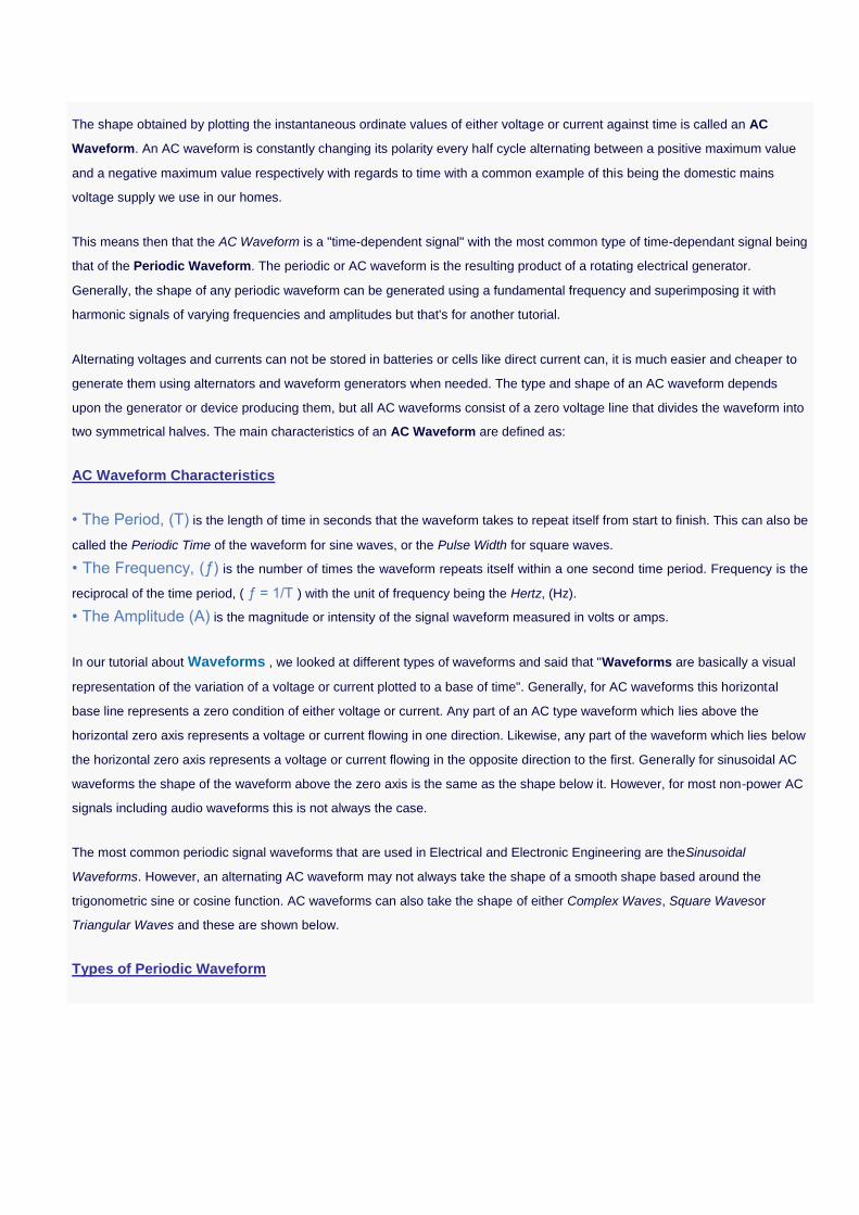
The most common periodic signal waveforms that are used in Electrical and Electronic Engineering are theSinusoidal

Waveforms. However, an alternating AC waveform may not always take the shape of a smooth shape based around the

trigonometric sine or cosine function. AC waveforms can also take the shape of either Complex Waves, Square Wavesor

Triangular Waves and these are shown below.

Types of Periodic Waveform

The time taken for an AC Waveform to complete one full pattern from its positive half to its negative half and back to its zero

baseline again is called a Cycle and one complete cycle contains both a positive half-cycle and a negative half-cycle. The time

taken by the waveform to complete one full cycle is called thePeriodic Time of the waveform, and is given the symbol T. The

number of complete cycles that are produced within one second (cycles/second) is called the Frequency, symbolƒ of the

alternating waveform. Frequency is measured in Hertz, ( Hz ) named after the German physicist Heinrich Hertz.

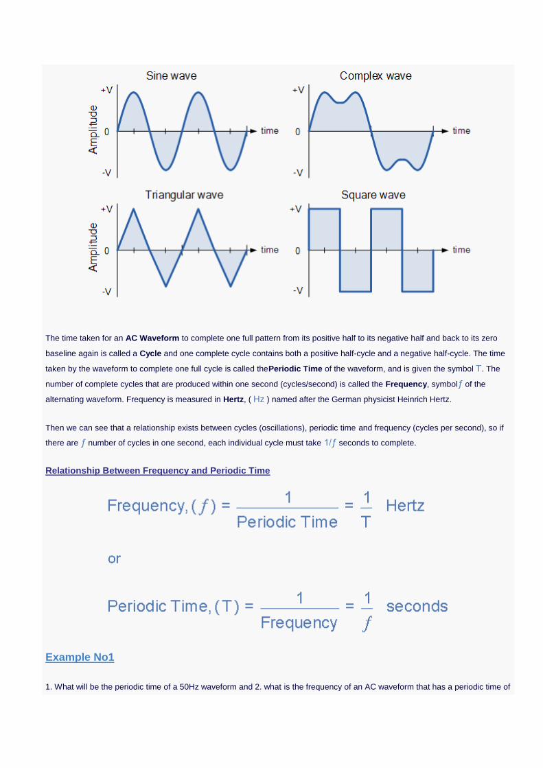
Then we can see that a relationship exists between cycles (oscillations), periodic time and frequency (cycles per second), so if

there are ƒ number of cycles in one second, each individual cycle must take 1/ƒ seconds to complete.

Relationship Between Frequency and Periodic Time

Example No1

1. What will be the periodic time of a 50Hz waveform and 2. what is the frequency of an AC waveform that has a periodic time of

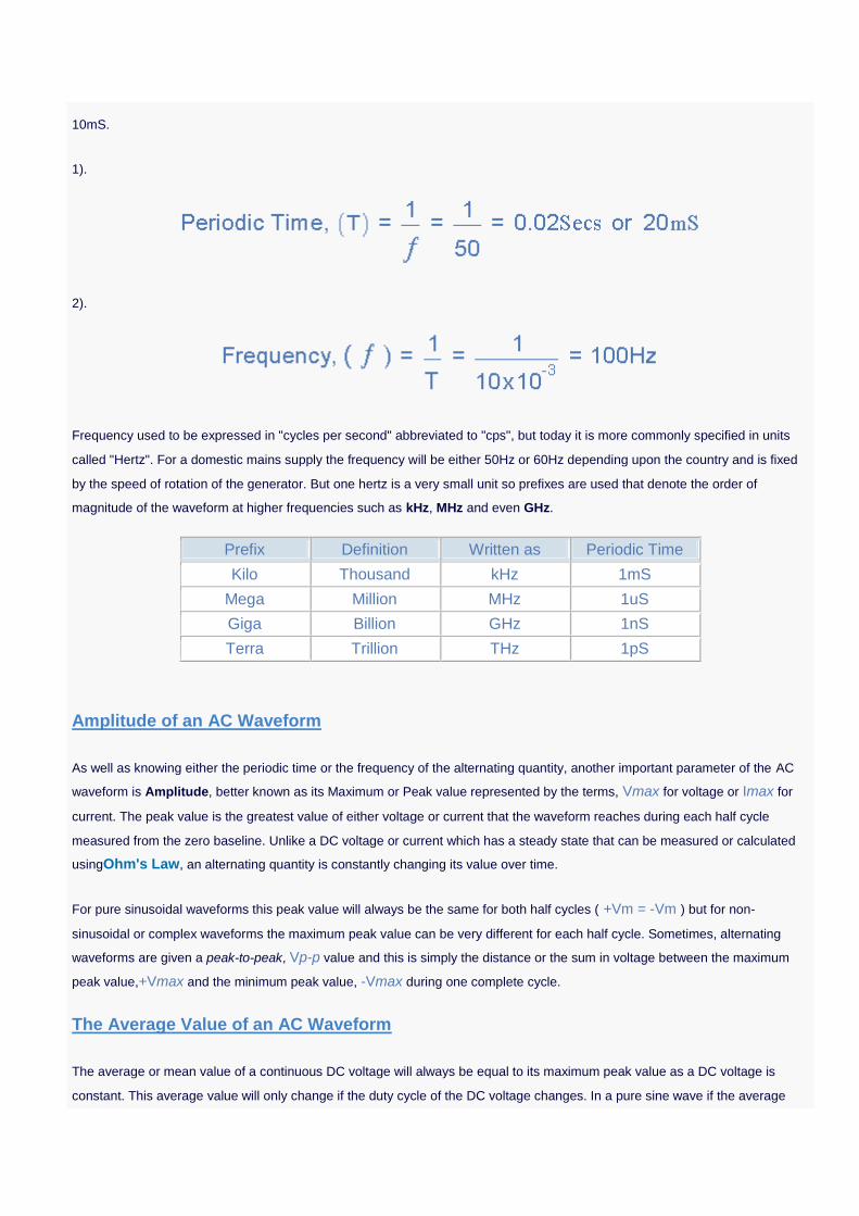
10mS.

1).

2).

Frequency used to be expressed in "cycles per second" abbreviated to "cps", but today it is more commonly specified in units

called "Hertz". For a domestic mains supply the frequency will be either 50Hz or 60Hz depending upon the country and is fixed

by the speed of rotation of the generator. But one hertz is a very small unit so prefixes are used that denote the order of

magnitude of the waveform at higher frequencies such as kHz, MHz and even GHz.

Prefix Definition Written as Periodic Time

Kilo Thousand kHz 1mS

Mega Million MHz 1uS

Giga Billion GHz 1nS

Terra Trillion THz 1pS

Amplitude of an AC Waveform

As well as knowing either the periodic time or the frequency of the alternating quantity, another important parameter of the AC

waveform is Amplitude, better known as its Maximum or Peak value represented by the terms, Vmax for voltage or Imax for

current. The peak value is the greatest value of either voltage or current that the waveform reaches during each half cycle

measured from the zero baseline. Unlike a DC voltage or current which has a steady state that can be measured or calculated

usingOhm's Law, an alternating quantity is constantly changing its value over time.

For pure sinusoidal waveforms this peak value will always be the same for both half cycles ( +Vm = -Vm ) but for non-

sinusoidal or complex waveforms the maximum peak value can be very different for each half cycle. Sometimes, alternating

waveforms are given a peak-to-peak, Vp-p value and this is simply the distance or the sum in voltage between the maximum

peak value,+Vmax and the minimum peak value, -Vmax during one complete cycle.

The Average Value of an AC Waveform

The average or mean value of a continuous DC voltage will always be equal to its maximum peak value as a DC voltage is

constant. This average value will only change if the duty cycle of the DC voltage changes. In a pure sine wave if the average

value is calculated over the full cycle, the average value would be equal to zero as the positive and negative halves will cancel

each other out. So the average or mean value of an AC waveform is calculated or measured over a half cycle only and this is

shown below.

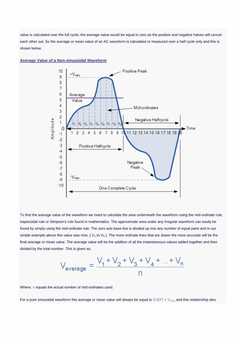
Average Value of a Non-sinusoidal Waveform

To find the average value of the waveform we need to calculate the area underneath the waveform using the mid-ordinate rule,

trapezoidal rule or Simpson's rule found in mathematics. The approximate area under any irregular waveform can easily be

found by simply using the mid-ordinate rule. The zero axis base line is divided up into any number of equal parts and in our

simple example above this value was nine, ( V1 to V9 ). The more ordinate lines that are drawn the more accurate will be the

final average or mean value. The average value will be the addition of all the instantaneous values added together and then

divided by the total number. This is given as.

Where: n equals the actual number of mid-ordinates used.

For a pure sinusoidal waveform this average or mean value will always be equal to 0.637 x Vmax and this relationship also

holds true for average values of current.

The RMS Value of an AC Waveform

The average value of an AC waveform is NOT the same value as that for a DC waveforms average value. This is because the

AC waveform is constantly changing with time and the heating effect given by the formula ( P = I 2.R ), will also be changing

producing a positive power consumption. The equivalent average value for an alternating current system that provides the same

power to the load as a DC equivalent circuit is called the "effective value".

This effective power in an alternating current system is therefore equal to: ( I 2.R.Average ). As power is proportional to current

squared, the effective current,I will be equal to √ I 2 Ave. Therefore, the effective current in an AC system is called the Root

Mean Squared or R.M.S. value and RMS values are the DC equivalent values that provide the same power to the load.

The effective or RMS value of an alternating current is measured in terms of the direct current value that produces the same

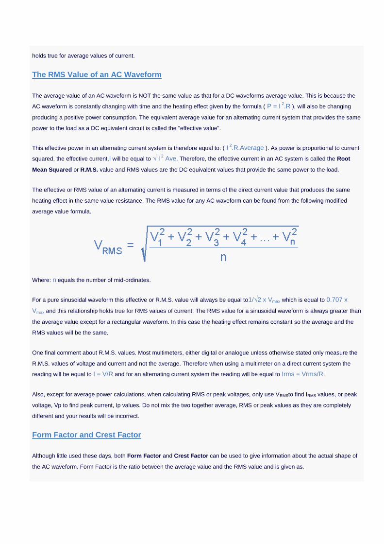
heating effect in the same value resistance. The RMS value for any AC waveform can be found from the following modified

average value formula.

Where: n equals the number of mid-ordinates.

For a pure sinusoidal waveform this effective or R.M.S. value will always be equal to1/√2 x Vmax which is equal to 0.707 x

Vmax and this relationship holds true for RMS values of current. The RMS value for a sinusoidal waveform is always greater than

the average value except for a rectangular waveform. In this case the heating effect remains constant so the average and the

RMS values will be the same.

One final comment about R.M.S. values. Most multimeters, either digital or analogue unless otherwise stated only measure the

R.M.S. values of voltage and current and not the average. Therefore when using a multimeter on a direct current system the

reading will be equal to I = V/R and for an alternating current system the reading will be equal to Irms = Vrms/R.

Also, except for average power calculations, when calculating RMS or peak voltages, only use VRMSto find IRMS values, or peak

voltage, Vp to find peak current, Ip values. Do not mix the two together average, RMS or peak values as they are completely

different and your results will be incorrect.

Form Factor and Crest Factor

Although little used these days, both Form Factor and Crest Factor can be used to give information about the actual shape of

the AC waveform. Form Factor is the ratio between the average value and the RMS value and is given as.

For a pure sinusoidal waveform the Form Factor will always be equal to 1.11.

Crest Factor is the ratio between the R.M.S. value and the Peak value of the waveform and is given as.

For a pure sinusoidal waveform the Crest Factor will always be equal to 1.414.

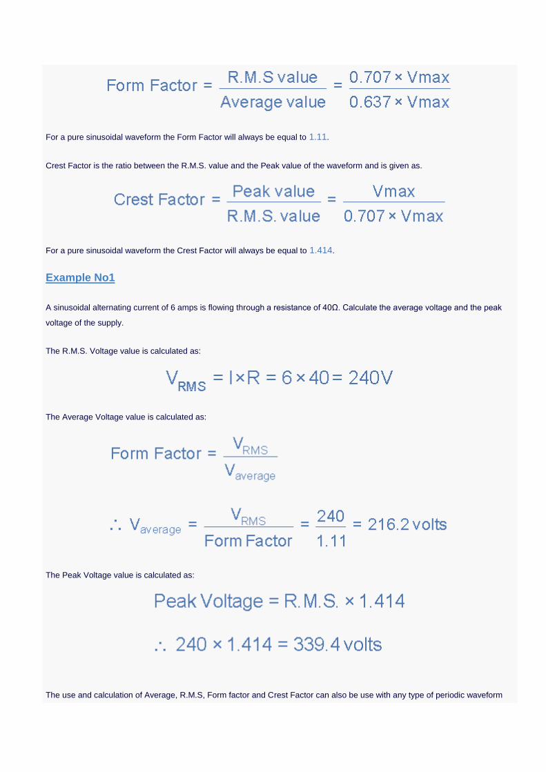
Example No1

A sinusoidal alternating current of 6 amps is flowing through a resistance of 40Ω. Calculate the average voltage and the peak

voltage of the supply.

The R.M.S. Voltage value is calculated as:

The Average Voltage value is calculated as:

The Peak Voltage value is calculated as:

The use and calculation of Average, R.M.S, Form factor and Crest Factor can also be use with any type of periodic waveform

including Triangular, Square, Sawtoothed or any other irregular or complex voltage/current waveform shape and in the next

tutorial about Sinusoidal Waveformswe will look at the principal of generating a sinusoidal AC waveform (a sinusoid) along

with its angular velocity representation.

The Sinusoidal Waveform Navigation

Tutorial: 2 of 12

--- Select a Tutorial Page ---

RESET

Generation of a Sinusoidal Waveform

In our tutorials about Electromagnetism, we saw how an electric current flowing through a conductor can be used to generate a

magnetic field around itself, and also if a single wire conductor is moved or rotated within a stationary magnetic field, an "EMF",

(Electro-Motive Force) will be induced within the conductor due to this movement. From this tutorial we learnt that a relationship exists

between Electricity and Magnetism giving us, as Michael Faraday discovered the effect of "Electromagnetic Induction" and it is this

basic principal that is used to generate a Sinusoidal Waveform.

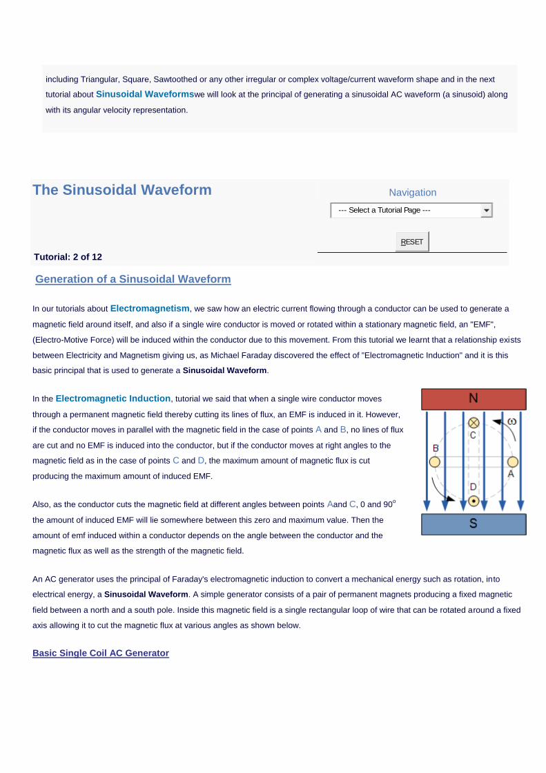
In the Electromagnetic Induction, tutorial we said that when a single wire conductor moves

through a permanent magnetic field thereby cutting its lines of flux, an EMF is induced in it. However,

if the conductor moves in parallel with the magnetic field in the case of points A and B, no lines of flux

are cut and no EMF is induced into the conductor, but if the conductor moves at right angles to the

magnetic field as in the case of points C and D, the maximum amount of magnetic flux is cut

producing the maximum amount of induced EMF.

Also, as the conductor cuts the magnetic field at different angles between points Aand C, 0 and 90o

the amount of induced EMF will lie somewhere between this zero and maximum value. Then the

amount of emf induced within a conductor depends on the angle between the conductor and the

magnetic flux as well as the strength of the magnetic field.

An AC generator uses the principal of Faraday's electromagnetic induction to convert a mechanical energy such as rotation, into

electrical energy, a Sinusoidal Waveform. A simple generator consists of a pair of permanent magnets producing a fixed magnetic

field between a north and a south pole. Inside this magnetic field is a single rectangular loop of wire that can be rotated around a fixed

axis allowing it to cut the magnetic flux at various angles as shown below.

Basic Single Coil AC Generator

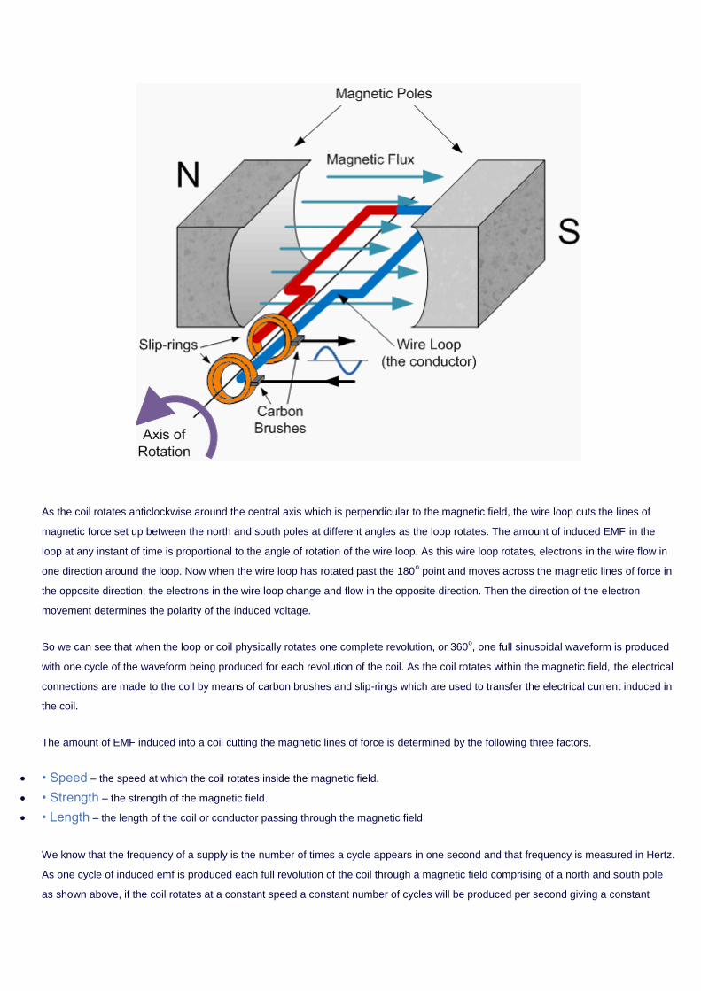
As the coil rotates anticlockwise around the central axis which is perpendicular to the magnetic field, the wire loop cuts the lines of

magnetic force set up between the north and south poles at different angles as the loop rotates. The amount of induced EMF in the

loop at any instant of time is proportional to the angle of rotation of the wire loop. As this wire loop rotates, electrons in the wire flow in

one direction around the loop. Now when the wire loop has rotated past the 180o point and moves across the magnetic lines of force in

the opposite direction, the electrons in the wire loop change and flow in the opposite direction. Then the direction of the electron

movement determines the polarity of the induced voltage.

So we can see that when the loop or coil physically rotates one complete revolution, or 360o, one full sinusoidal waveform is produced

with one cycle of the waveform being produced for each revolution of the coil. As the coil rotates within the magnetic field, the electrical

connections are made to the coil by means of carbon brushes and slip-rings which are used to transfer the electrical current induced in

the coil.

The amount of EMF induced into a coil cutting the magnetic lines of force is determined by the following three factors.

• Speed – the speed at which the coil rotates inside the magnetic field.

• Strength – the strength of the magnetic field.

• Length – the length of the coil or conductor passing through the magnetic field.

We know that the frequency of a supply is the number of times a cycle appears in one second and that frequency is measured in Hertz.

As one cycle of induced emf is produced each full revolution of the coil through a magnetic field comprising of a north and south pole

as shown above, if the coil rotates at a constant speed a constant number of cycles will be produced per second giving a constant

frequency. So by increasing the speed of rotation of the coil the frequency will also be increased. Therefore, frequency is proportional

to the speed of rotation, ( ƒ ∝ Ν ) where Ν = r.p.m.

Also, our simple single coil generator above only has two poles, one north and one south pole, giving just one pair of poles. If we add

more magnetic poles to the generator above so that it now has four poles in total, two north and two south, then for each revolution of

the coil two cycles will be produced for the same rotational speed. Therefore, frequency is proportional to the number of pairs of

magnetic poles, ( ƒ ∝ P ) of the generator where P = is the number of "pairs of poles".

Then from these two facts we can say that the frequency output from an AC generator is:

Where: Ν is the speed of rotation in r.p.m. P is the number of "pairs of poles" and 60 converts it into seconds.

Instantaneous Voltage

The EMF induced in the coil at any instant of time depends upon the rate or speed at which the coil cuts the lines of magnetic flux

between the poles and this is dependant upon the angle of rotation, Theta ( θ ) of the generating device. Because an AC waveform is

constantly changing its value or amplitude, the waveform at any instant in time will have a different value from its next instant in time.

For example, the value at 1ms will be different to the value at 1.2ms and so on. These values are known generally as the

Instantaneous Values, or Vi Then the instantaneous value of the waveform and also its direction will vary according to the position of

the coil within the magnetic field as shown below.

Displacement of a Coil within a Magnetic Field

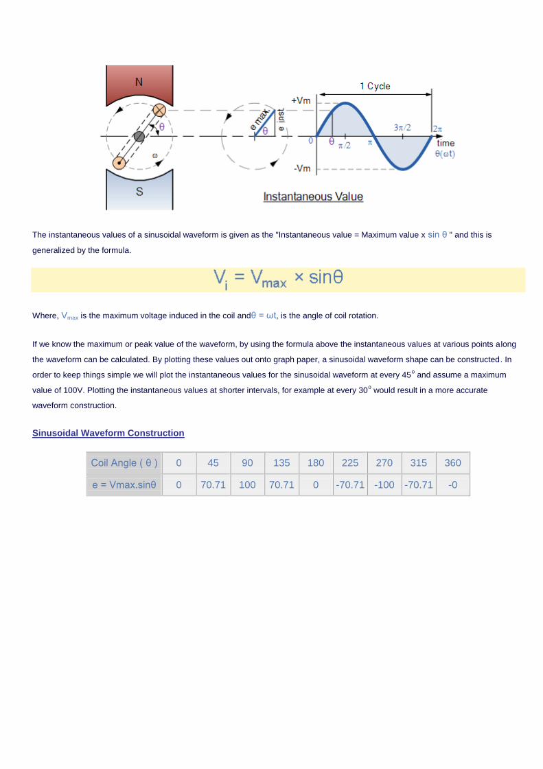
The instantaneous values of a sinusoidal waveform is given as the "Instantaneous value = Maximum value x sin θ " and this is

generalized by the formula.

Where, Vmax is the maximum voltage induced in the coil andθ = ωt, is the angle of coil rotation.

If we know the maximum or peak value of the waveform, by using the formula above the instantaneous values at various points along

the waveform can be calculated. By plotting these values out onto graph paper, a sinusoidal waveform shape can be constructed. In

order to keep things simple we will plot the instantaneous values for the sinusoidal waveform at every 45o and assume a maximum

value of 100V. Plotting the instantaneous values at shorter intervals, for example at every 30o would result in a more accurate

waveform construction.

Sinusoidal Waveform Construction

Coil Angle ( θ ) 0 45 90 135 180 225 270 315 360

e = Vmax.sinθ 0 70.71 100 70.71 0 -70.71 -100 -70.71 -0

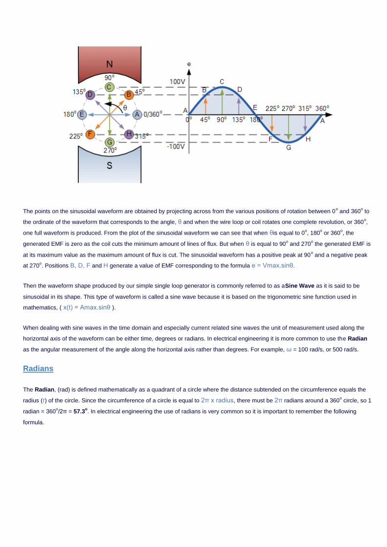
The points on the sinusoidal waveform are obtained by projecting across from the various positions of rotation between 0o and 360

o to

the ordinate of the waveform that corresponds to the angle, θ and when the wire loop or coil rotates one complete revolution, or 360o,

one full waveform is produced. From the plot of the sinusoidal waveform we can see that when θis equal to 0o, 180

o or 360

o, the

generated EMF is zero as the coil cuts the minimum amount of lines of flux. But when θ is equal to 90o and 270

o the generated EMF is

at its maximum value as the maximum amount of flux is cut. The sinusoidal waveform has a positive peak at 90o and a negative peak

at 270o. Positions B, D, F and H generate a value of EMF corresponding to the formula e = Vmax.sinθ.

Then the waveform shape produced by our simple single loop generator is commonly referred to as aSine Wave as it is said to be

sinusoidal in its shape. This type of waveform is called a sine wave because it is based on the trigonometric sine function used in

mathematics, ( x(t) = Amax.sinθ ).

When dealing with sine waves in the time domain and especially current related sine waves the unit of measurement used along the

horizontal axis of the waveform can be either time, degrees or radians. In electrical engineering it is more common to use the Radian

as the angular measurement of the angle along the horizontal axis rather than degrees. For example, ω = 100 rad/s, or 500 rad/s.

Radians

The Radian, (rad) is defined mathematically as a quadrant of a circle where the distance subtended on the circumference equals the

radius (r) of the circle. Since the circumference of a circle is equal to 2π x radius, there must be 2π radians around a 360o circle, so 1

radian = 360o/2π = 57.3

o. In electrical engineering the use of radians is very common so it is important to remember the following

formula.

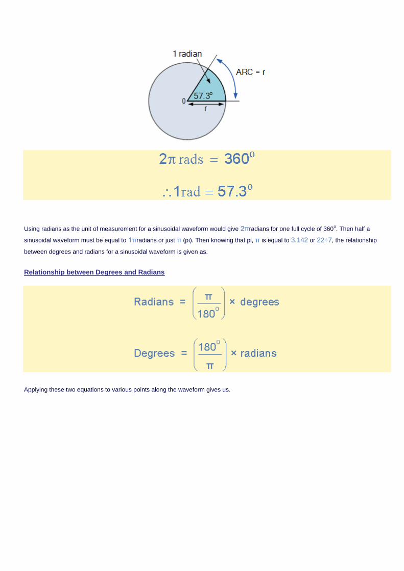
Using radians as the unit of measurement for a sinusoidal waveform would give 2πradians for one full cycle of 360o. Then half a

sinusoidal waveform must be equal to 1πradians or just π (pi). Then knowing that pi, π is equal to 3.142 or 22÷7, the relationship

between degrees and radians for a sinusoidal waveform is given as.

Relationship between Degrees and Radians

Applying these two equations to various points along the waveform gives us.

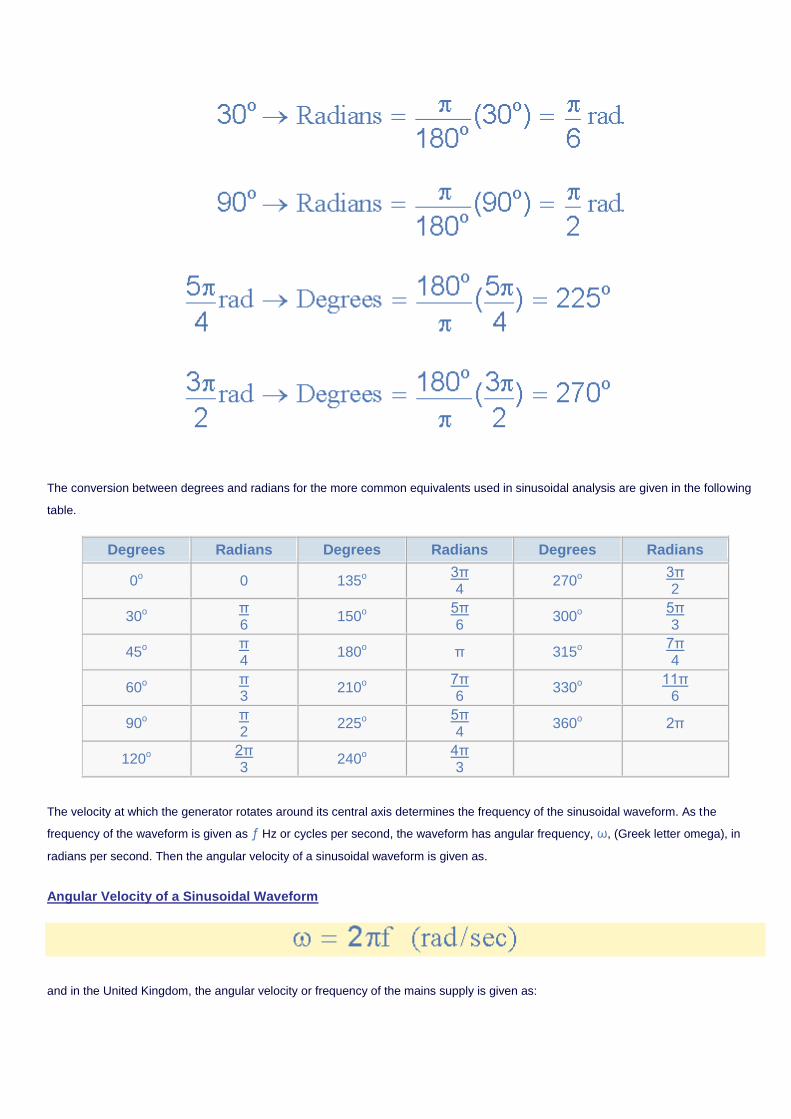
The conversion between degrees and radians for the more common equivalents used in sinusoidal analysis are given in the following

table.

Degrees Radians Degrees Radians Degrees Radians

0o 0 135o 3π 4

270o 3π 2

30o π 6

150o 5π 6

300o 5π 3

45o π 4

180o π 315o 7π 4

60o π 3

210o 7π 6

330o 11π

6

90o π 2

225o 5π 4

360o 2π

120o 2π 3

240o 4π 3

The velocity at which the generator rotates around its central axis determines the frequency of the sinusoidal waveform. As the

frequency of the waveform is given as ƒ Hz or cycles per second, the waveform has angular frequency, ω, (Greek letter omega), in

radians per second. Then the angular velocity of a sinusoidal waveform is given as.

Angular Velocity of a Sinusoidal Waveform

and in the United Kingdom, the angular velocity or frequency of the mains supply is given as:

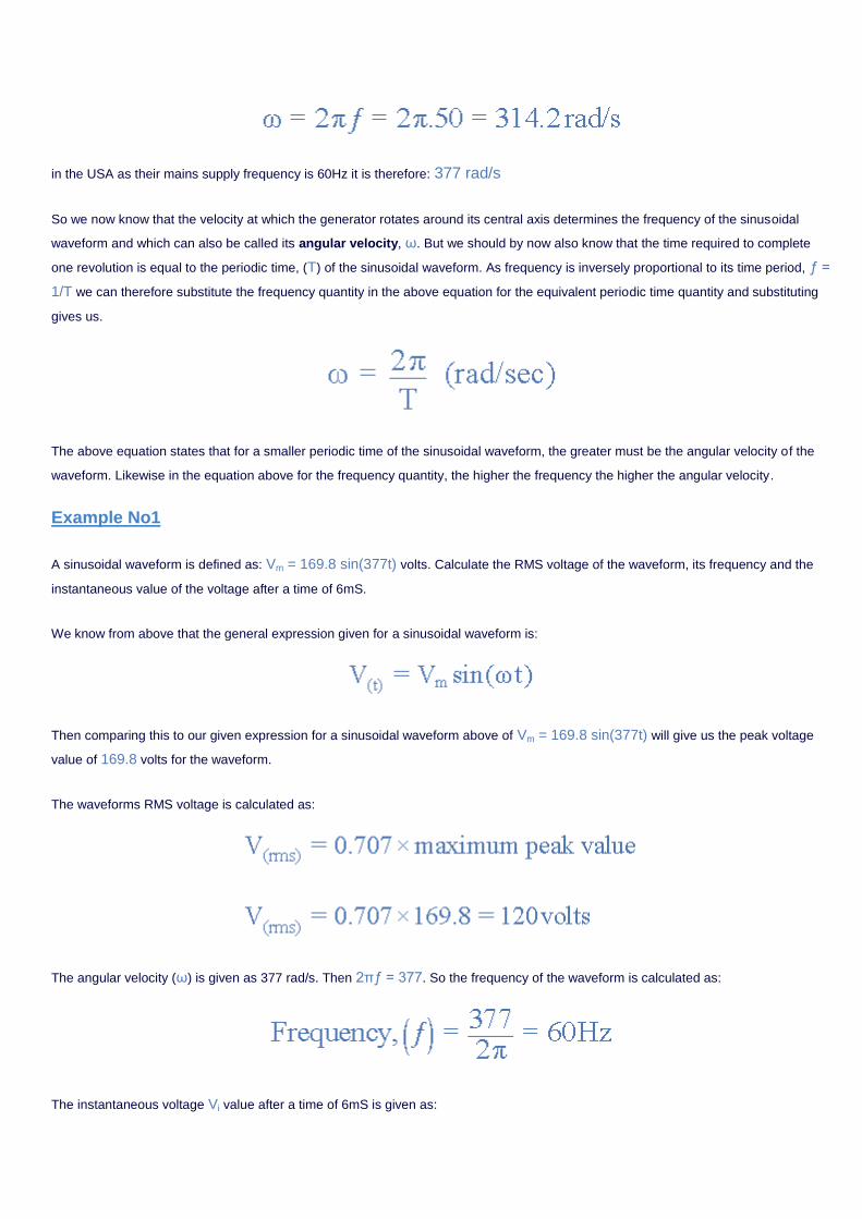
in the USA as their mains supply frequency is 60Hz it is therefore: 377 rad/s

So we now know that the velocity at which the generator rotates around its central axis determines the frequency of the sinusoidal

waveform and which can also be called its angular velocity, ω. But we should by now also know that the time required to complete

one revolution is equal to the periodic time, (T) of the sinusoidal waveform. As frequency is inversely proportional to its time period, ƒ =

1/T we can therefore substitute the frequency quantity in the above equation for the equivalent periodic time quantity and substituting

gives us.

The above equation states that for a smaller periodic time of the sinusoidal waveform, the greater must be the angular velocity of the

waveform. Likewise in the equation above for the frequency quantity, the higher the frequency the higher the angular velocity.

Example No1

A sinusoidal waveform is defined as: Vm = 169.8 sin(377t) volts. Calculate the RMS voltage of the waveform, its frequency and the

instantaneous value of the voltage after a time of 6mS.

We know from above that the general expression given for a sinusoidal waveform is:

Then comparing this to our given expression for a sinusoidal waveform above of Vm = 169.8 sin(377t) will give us the peak voltage

value of 169.8 volts for the waveform.

The waveforms RMS voltage is calculated as:

The angular velocity (ω) is given as 377 rad/s. Then 2πƒ = 377. So the frequency of the waveform is calculated as:

The instantaneous voltage Vi value after a time of 6mS is given as:

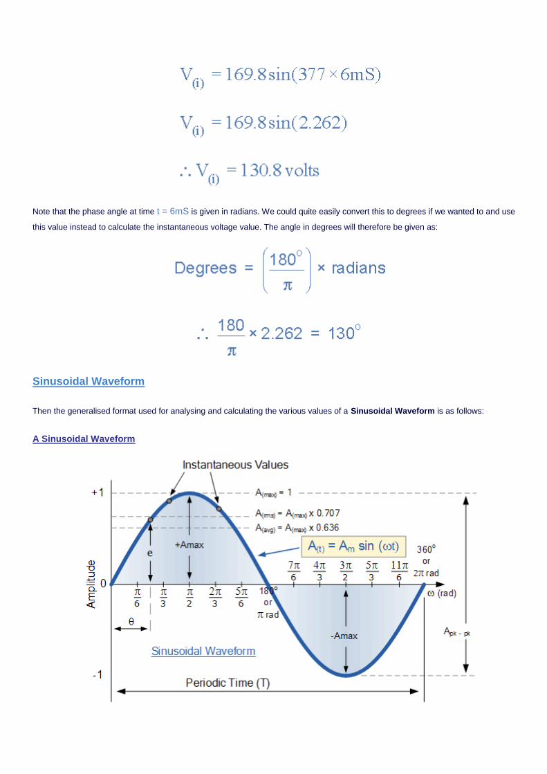
Note that the phase angle at time t = 6mS is given in radians. We could quite easily convert this to degrees if we wanted to and use

this value instead to calculate the instantaneous voltage value. The angle in degrees will therefore be given as:

Sinusoidal Waveform

Then the generalised format used for analysing and calculating the various values of a Sinusoidal Waveform is as follows:

A Sinusoidal Waveform

In the next tutorial aboutPhase Difference we will look at the relationship between two sinusoidal waveforms that are of the same

frequency but pass through the horizontal zero axis at different time intervals.

Phase Difference Navigation

Tutorial: 3 of 12

--- Select a Tutorial Page ---

RESET

Phase Difference

In the last tutorial, we saw that theSinusoidal Waveform (Sine Wave) can be presented graphically in the time domain along an

horizontal zero axis, and that sine waves have a positive maximum value at time π/2, a negative maximum value at time 3π/2, with

zero values occurring along the baseline at0, π and 2π. However, not all sinusoidal waveforms will pass exactly through the zero axis

point at the same time, but may be "shifted" to the right or to the left of 0o by some value when compared to another sine wave. For

example, comparing a voltage waveform to that of a current waveform. This then produces an angular shift or Phase Difference

between the two sinusoidal waveforms. Any sine wave that does not pass through zero at t = 0 has a phase shift.

The phase difference or phase shift as it is also called of a sinusoidal waveform is the angle Φ (Greek letter Phi), in degrees or

radians that the waveform has shifted from a certain reference point along the horizontal zero axis. In other words phase shift is the

lateral difference between two or more waveforms along a common axis and sinusoidal waveforms of the same frequency can have a

phase difference.

The phase difference, Φ of an alternating waveform can vary from between0 to its maximum time period, T of the waveform during one

complete cycle and this can be anywhere along the horizontal axis between,Φ = 0 to 2π(radians) or Φ = 0 to 360o depending upon

the angular units used. Phase difference can also be expressed as a time shift of τ in seconds representing a fraction of the time

period, T for example, +10mS or - 50uS but generally it is more common to express phase difference as an angular measurement.

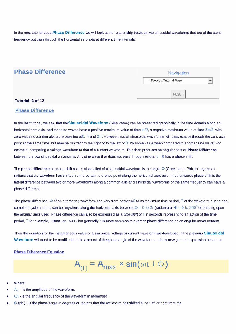
Then the equation for the instantaneous value of a sinusoidal voltage or current waveform we developed in the previous Sinusoidal

Waveform will need to be modified to take account of the phase angle of the waveform and this new general expression becomes.

Phase Difference Equation

Where:

Am - is the amplitude of the waveform.

ωt - is the angular frequency of the waveform in radian/sec.

Φ (phi) - is the phase angle in degrees or radians that the waveform has shifted either left or right from the

reference point.

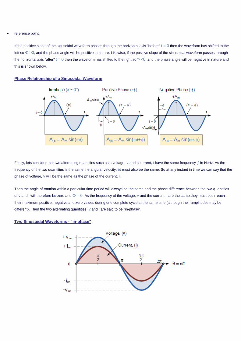
If the positive slope of the sinusoidal waveform passes through the horizontal axis "before" t = 0 then the waveform has shifted to the

left so Φ >0, and the phase angle will be positive in nature. Likewise, if the positive slope of the sinusoidal waveform passes through

the horizontal axis "after" t = 0 then the waveform has shifted to the right soΦ <0, and the phase angle will be negative in nature and

this is shown below.

Phase Relationship of a Sinusoidal Waveform

Firstly, lets consider that two alternating quantities such as a voltage, v and a current, i have the same frequency ƒ in Hertz. As the

frequency of the two quantities is the same the angular velocity, ω must also be the same. So at any instant in time we can say that the

phase of voltage, v will be the same as the phase of the current, i.

Then the angle of rotation within a particular time period will always be the same and the phase difference between the two quantities

of v and i will therefore be zero and Φ = 0. As the frequency of the voltage, v and the current, i are the same they must both reach

their maximum positive, negative and zero values during one complete cycle at the same time (although their amplitudes may be

different). Then the two alternating quantities, v and i are said to be "in-phase".

Two Sinusoidal Waveforms - "in-phase"

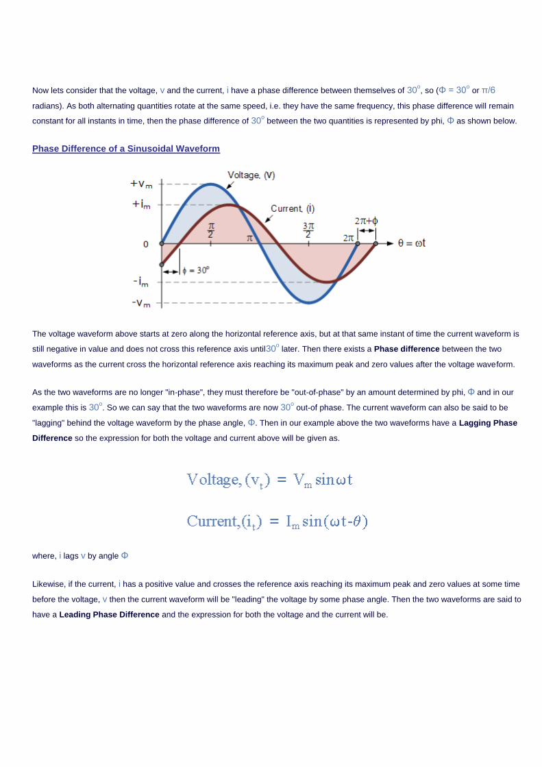
Now lets consider that the voltage, v and the current, i have a phase difference between themselves of 30o, so (Φ = 30

o or π/6

radians). As both alternating quantities rotate at the same speed, i.e. they have the same frequency, this phase difference will remain

constant for all instants in time, then the phase difference of 30o between the two quantities is represented by phi, Φ as shown below.

Phase Difference of a Sinusoidal Waveform

The voltage waveform above starts at zero along the horizontal reference axis, but at that same instant of time the current waveform is

still negative in value and does not cross this reference axis until30o later. Then there exists a Phase difference between the two

waveforms as the current cross the horizontal reference axis reaching its maximum peak and zero values after the voltage waveform.

As the two waveforms are no longer "in-phase", they must therefore be "out-of-phase" by an amount determined by phi, Φ and in our

example this is 30o. So we can say that the two waveforms are now 30

o out-of phase. The current waveform can also be said to be

"lagging" behind the voltage waveform by the phase angle, Φ. Then in our example above the two waveforms have a Lagging Phase

Difference so the expression for both the voltage and current above will be given as.

where, i lags v by angle Φ

Likewise, if the current, i has a positive value and crosses the reference axis reaching its maximum peak and zero values at some time

before the voltage, v then the current waveform will be "leading" the voltage by some phase angle. Then the two waveforms are said to

have a Leading Phase Difference and the expression for both the voltage and the current will be.

where, i leads v by angle Φ

The phase angle of a sine wave can be used to describe the relationship of one sine wave to another by using the terms "Leading" and

"Lagging" to indicate the relationship between two sinusoidal waveforms of the same frequency, plotted onto the same reference axis.

In our example above the two waveforms are out-of-phase by30o so we can say that i lags vor v leads i by 30

o.

The relationship between the two waveforms and the resulting phase angle can be measured anywhere along the horizontal zero axis

through which each waveform passes with the "same slope" direction either positive or negative. In AC power circuits this ability to

describe the relationship between a voltage and a current sine wave within the same circuit is very important and forms the bases of

AC circuit analysis.

The Cosine Waveform

So we now know that if a waveform is "shifted" to the right or left of 0owhen compared to another sine wave the expression for this

waveform becomesAm sin(ωt ± Φ). But if the waveform crosses the horizontal zero axis with a positive going slope 90o or π/2 radians

before the reference waveform, the waveform is called a Cosine Waveform and the expression becomes.

Cosine Expression

The Cosine Wave, simply called "cos", is as important as the sine wave in electrical engineering. The cosine wave has the same

shape as its sine wave counterpart that is it is a sinusoidal function, but is shifted by +90o or one full quarter of a period ahead of it.

Phase Difference between a Sine wave and a Cosine wave

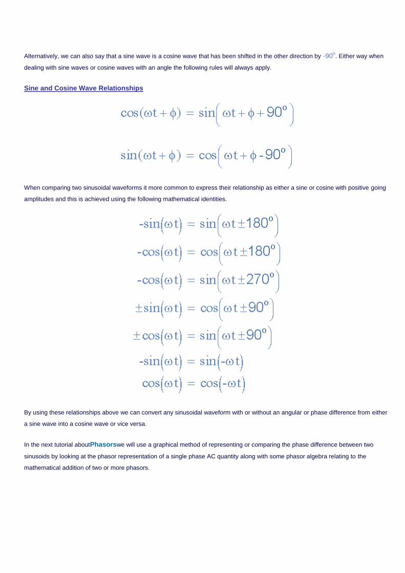
Alternatively, we can also say that a sine wave is a cosine wave that has been shifted in the other direction by -90o. Either way when

dealing with sine waves or cosine waves with an angle the following rules will always apply.

Sine and Cosine Wave Relationships

When comparing two sinusoidal waveforms it more common to express their relationship as either a sine or cosine with positive going

amplitudes and this is achieved using the following mathematical identities.

By using these relationships above we can convert any sinusoidal waveform with or without an angular or phase difference from either

a sine wave into a cosine wave or vice versa.

In the next tutorial aboutPhasorswe will use a graphical method of representing or comparing the phase difference between two

sinusoids by looking at the phasor representation of a single phase AC quantity along with some phasor algebra relating to the

mathematical addition of two or more phasors.

Phasor Diagram Navigation

Tutorial: 4 of 12

--- Select a Tutorial Page ---

RESET

The Phasor Diagram

In the last tutorial, we saw that sinusoidal waveforms of the same frequency can have aPhase Difference between themselves

which represents the angular difference of the two sinusoidal waveforms. Also the terms "lead" and "lag" as well as "in-phase" and "out-

of-phase" were used to indicate the relationship of one waveform to the other with the generalized sinusoidal expression given as: A(t)

= Am sin(ωt ± Φ)representing the sinusoid in the time-domain form. But when presented mathematically in this way it is sometimes

difficult to visualise this angular or phase difference between two or more sinusoidal waveforms so sinusoids can also be represented

graphically in the spacial or phasor-domain form by a Phasor Diagram, and this is achieved by using the rotating vector method.

Basically a rotating vector, simply called a "Phasor" is a scaled line whose length represents an AC quantity that has both magnitude

("peak amplitude") and direction ("phase") which is "frozen" at some point in time. A phasor is a vector that has an arrow head at one

end which signifies partly the maximum value of the vector quantity ( V or I ) and partly the end of the vector that rotates.

Generally, vectors are assumed to pivot at one end around a fixed zero point known as the "point of origin" while the arrowed end

representing the quantity, freely rotates in ananti-clockwise direction at an angular velocity, ( ω ) of one full revolution for every cycle.

This anti-clockwise rotation of the vector is considered to be a positive rotation. Likewise, a clockwise rotation is considered to be a

negative rotation.

Although the both the terms vectors and phasors are used to describe a rotating line that itself has both magnitude and direction, the

main difference between the two is that a vectors magnitude is the "peak value" of the sinusoid while a phasors magnitude is the "rms

value" of the sinusoid. In both cases the phase angle and direction remains the same.

The phase of an alternating quantity at any instant in time can be represented by a phasor diagram, so phasor diagrams can be

thought of as "functions of time". A complete sine wave can be constructed by a single vector rotating at an angular velocity of ω =

2πƒ, where ƒ is the frequency of the waveform. Then a Phasor is a quantity that has both "Magnitude" and "Direction". Generally,

when constructing a phasor diagram, angular velocity of a sine wave is always assumed to be: ω in rad/s. Consider the phasor

diagram below.

Phasor Diagram of a Sinusoidal Waveform

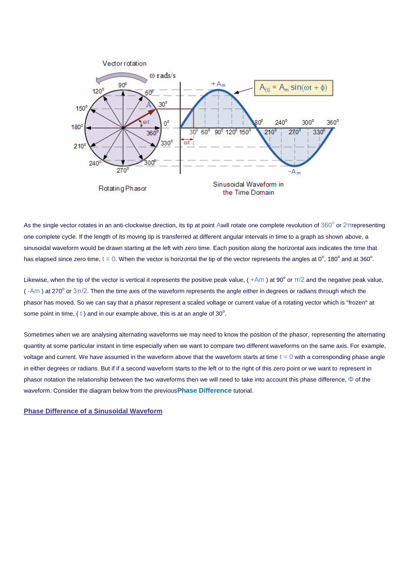
As the single vector rotates in an anti-clockwise direction, its tip at point Awill rotate one complete revolution of 360o or 2πrepresenting

one complete cycle. If the length of its moving tip is transferred at different angular intervals in time to a graph as shown above, a

sinusoidal waveform would be drawn starting at the left with zero time. Each position along the horizontal axis indicates the time that

has elapsed since zero time, t = 0. When the vector is horizontal the tip of the vector represents the angles at 0o, 180

o and at 360

o.

Likewise, when the tip of the vector is vertical it represents the positive peak value, ( +Am ) at 90o or π/2 and the negative peak value,

( -Am ) at 270o or 3π/2. Then the time axis of the waveform represents the angle either in degrees or radians through which the

phasor has moved. So we can say that a phasor represent a scaled voltage or current value of a rotating vector which is "frozen" at

some point in time, ( t ) and in our example above, this is at an angle of 30o.

Sometimes when we are analysing alternating waveforms we may need to know the position of the phasor, representing the alternating

quantity at some particular instant in time especially when we want to compare two different waveforms on the same axis. For example,

voltage and current. We have assumed in the waveform above that the waveform starts at time t = 0 with a corresponding phase angle

in either degrees or radians. But if if a second waveform starts to the left or to the right of this zero point or we want to represent in

phasor notation the relationship between the two waveforms then we will need to take into account this phase difference, Φ of the

waveform. Consider the diagram below from the previousPhase Difference tutorial.

Phase Difference of a Sinusoidal Waveform

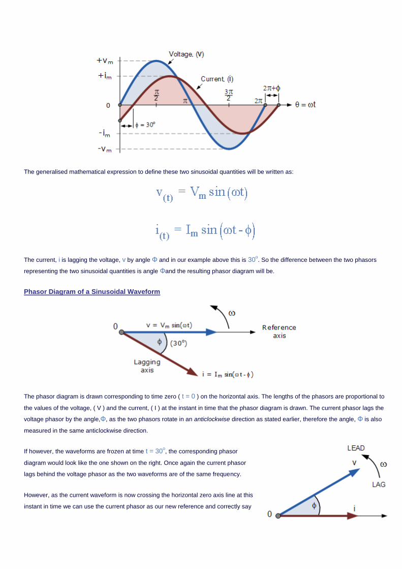
The generalised mathematical expression to define these two sinusoidal quantities will be written as:

The current, i is lagging the voltage, v by angle Φ and in our example above this is 30o. So the difference between the two phasors

representing the two sinusoidal quantities is angle Φand the resulting phasor diagram will be.

Phasor Diagram of a Sinusoidal Waveform

The phasor diagram is drawn corresponding to time zero ( t = 0 ) on the horizontal axis. The lengths of the phasors are proportional to

the values of the voltage, ( V ) and the current, ( I ) at the instant in time that the phasor diagram is drawn. The current phasor lags the

voltage phasor by the angle,Φ, as the two phasors rotate in an anticlockwise direction as stated earlier, therefore the angle, Φ is also

measured in the same anticlockwise direction.

If however, the waveforms are frozen at time t = 30o, the corresponding phasor

diagram would look like the one shown on the right. Once again the current phasor

lags behind the voltage phasor as the two waveforms are of the same frequency.

However, as the current waveform is now crossing the horizontal zero axis line at this

instant in time we can use the current phasor as our new reference and correctly say

that the voltage phasor is "leading" the current phasor by angle, Φ. Either way, one phasor is designated as the reference phasor and

all the other phasors will be either leading or lagging with respect to this reference.

Phasor Addition

Sometimes it is necessary when studying sinusoids to add together two alternating waveforms, for example in an AC series circuit, that

are not in-phase with each other. If they are in-phase that is, there is no phase shift then they can be added together in the same way

as DC values to find the algebraic sum of the two vectors. For example, two voltages in phase of say 50 volts and 25 volts respectively,

will sum together as one 75 volts voltage. If however, they are not in-phase that is, they do not have identical directions or starting point

then the phase angle between them needs to be taken into account so they are added together using phasor diagrams to determine

their Resultant Phasor or Vector Sum by using the parallelogram law.

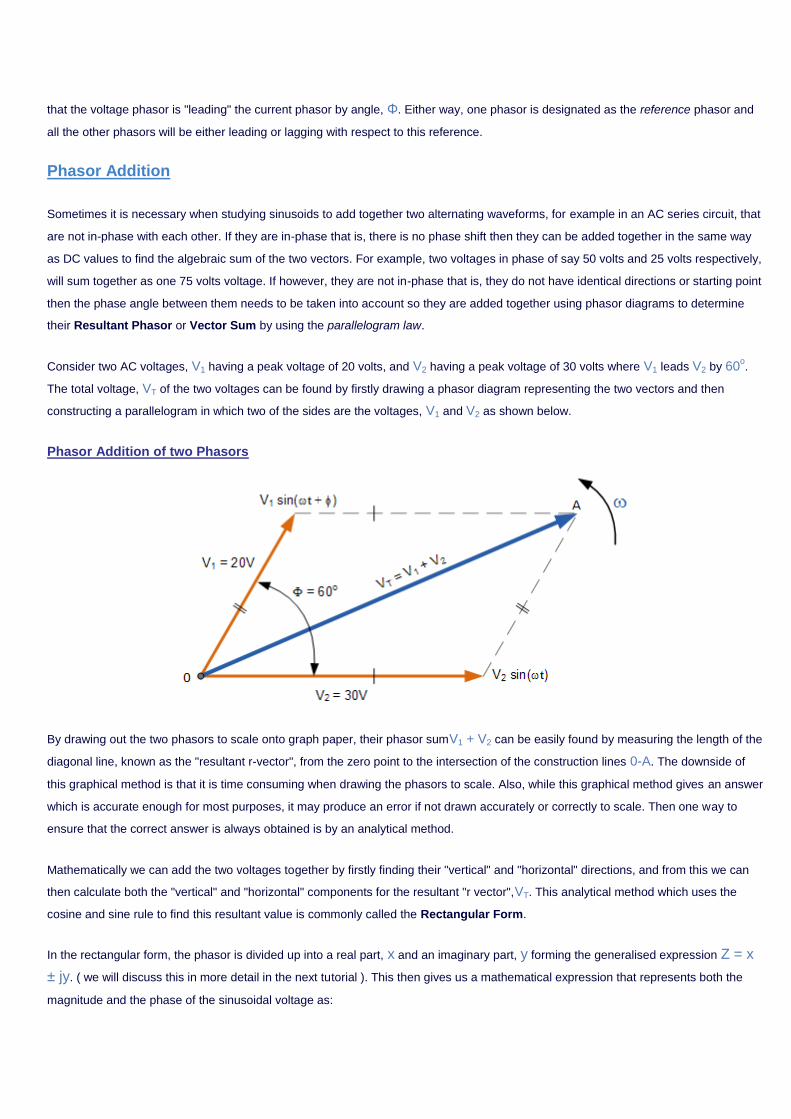
Consider two AC voltages, V1 having a peak voltage of 20 volts, and V2 having a peak voltage of 30 volts where V1 leads V2 by 60o.

The total voltage, VT of the two voltages can be found by firstly drawing a phasor diagram representing the two vectors and then

constructing a parallelogram in which two of the sides are the voltages, V1 and V2 as shown below.

Phasor Addition of two Phasors

By drawing out the two phasors to scale onto graph paper, their phasor sumV1 + V2 can be easily found by measuring the length of the

diagonal line, known as the "resultant r-vector", from the zero point to the intersection of the construction lines 0-A. The downside of

this graphical method is that it is time consuming when drawing the phasors to scale. Also, while this graphical method gives an answer

which is accurate enough for most purposes, it may produce an error if not drawn accurately or correctly to scale. Then one way to

ensure that the correct answer is always obtained is by an analytical method.

Mathematically we can add the two voltages together by firstly finding their "vertical" and "horizontal" directions, and from this we can

then calculate both the "vertical" and "horizontal" components for the resultant "r vector",VT. This analytical method which uses the

cosine and sine rule to find this resultant value is commonly called the Rectangular Form.

In the rectangular form, the phasor is divided up into a real part, x and an imaginary part, y forming the generalised expression Z = x

± jy. ( we will discuss this in more detail in the next tutorial ). This then gives us a mathematical expression that represents both the

magnitude and the phase of the sinusoidal voltage as:

So the addition of two vectors, A and B using the previous generalised expression is as follows:

Phasor Addition using Rectangular Form

Voltage, V2 of 30 volts points in the reference direction along the horizontal zero axis, then it has a horizontal component but no vertical

component as follows.

Horizontal component = 30 cos 0o = 30 volts

Vertical component = 30 sin 0o = 0 volts

This then gives us the rectangular expression for voltage V2 of: 30 + j0

Voltage, V1 of 20 volts leads voltage, V2 by 60o, then it has both horizontal and vertical components as follows.

Horizontal component = 20 cos 60o = 20 x 0.5 = 10 volts

Vertical component = 20 sin 60o = 20 x 0.866 = 17.32 volts

This then gives us the rectangular expression for voltage V1 of: 10 + j17.32

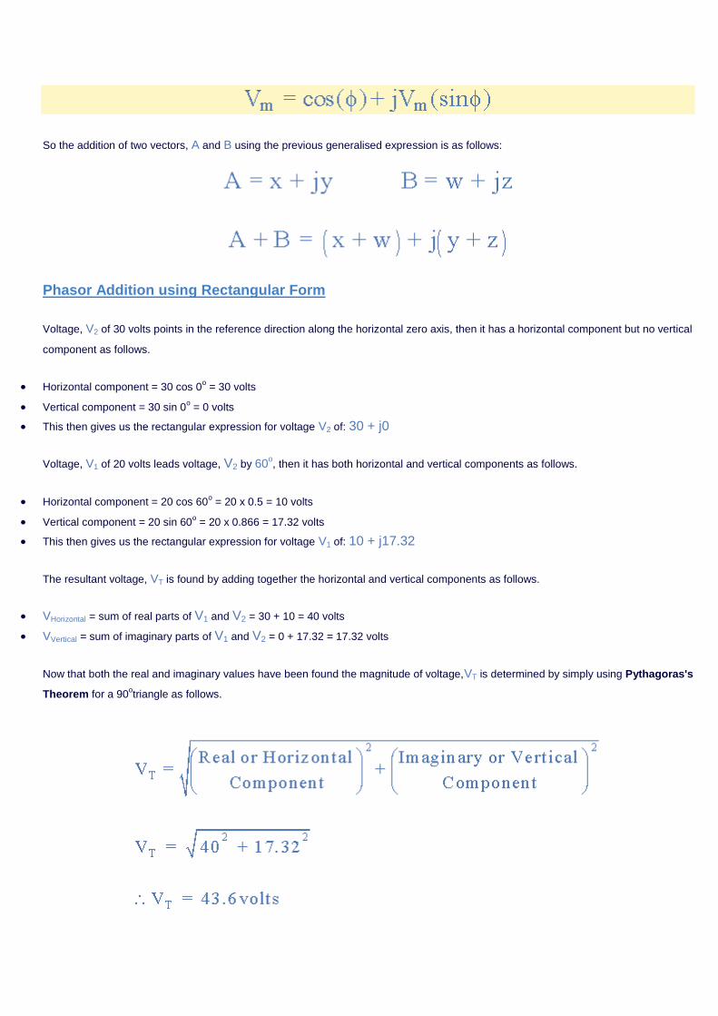
The resultant voltage, VT is found by adding together the horizontal and vertical components as follows.

VHorizontal = sum of real parts of V1 and V2 = 30 + 10 = 40 volts

VVertical = sum of imaginary parts of V1 and V2 = 0 + 17.32 = 17.32 volts

Now that both the real and imaginary values have been found the magnitude of voltage,VT is determined by simply using Pythagoras's

Theorem for a 90otriangle as follows.

Then the resulting phasor diagram will be:

Resultant Value of VT

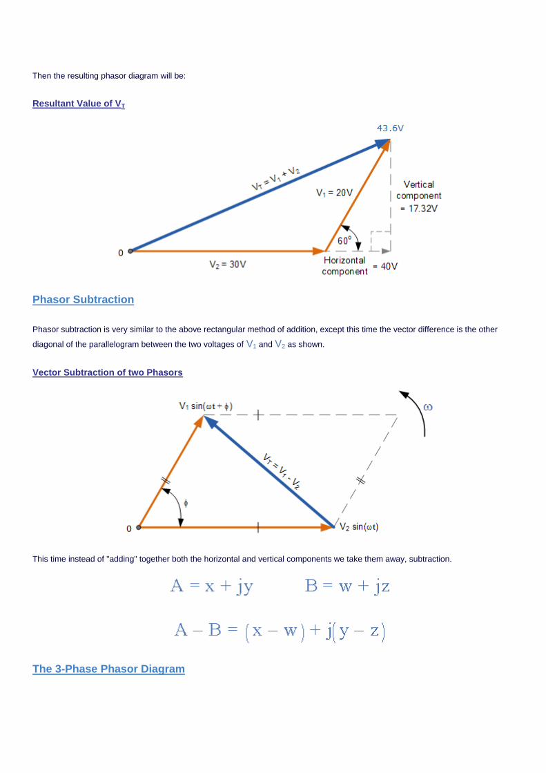
Phasor Subtraction

Phasor subtraction is very similar to the above rectangular method of addition, except this time the vector difference is the other

diagonal of the parallelogram between the two voltages of V1 and V2 as shown.

Vector Subtraction of two Phasors

This time instead of "adding" together both the horizontal and vertical components we take them away, subtraction.

The 3-Phase Phasor Diagram

Previously we have only looked at single-phase AC waveforms where a single multi turn coil rotates within a magnetic field. But if three

identical coils each with the same number of coil turns are placed at an electrical angle of 120o to each other on the same rotor shaft, a

three-phase voltage supply would be generated. A balanced three-phase voltage supply consists of three individual sinusoidal voltages

that are all equal in magnitude and frequency but are out-of-phase with each other by exactly 120o electrical degrees.

Standard practice is to colour code the three phases as Red,Yellow and Blue to identify each individual phase with the red phase as

the reference phase. The normal sequence of rotation for a three phase supply is Redfollowed by Yellow followed by Blue, ( R, Y, B ).

As with the single-phase phasors above, the phasors representing a three-phase system also rotate in an anti-clockwise direction

around a central point as indicated by the arrow marked ω in rad/s. The phasors for a three-phase balanced star or delta connected

system are shown below.

Three-phase Phasor Diagram

The phase voltages are all equal in magnitude but only differ in their phase angle. The three windings of the coils are connected

together at points, a1, b1 and c1 to produce a common neutral connection for the three individual phases. Then if the red phase is taken

as the reference phase each individual phase voltage can be defined with respect to the common neutral as.

Three-phase Voltage Equations

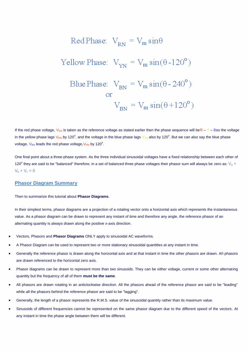
If the red phase voltage, VRN is taken as the reference voltage as stated earlier then the phase sequence will beR – Y – Bso the voltage

in the yellow phase lags VRN by 120o, and the voltage in the blue phase lags VYN also by 120

o. But we can also say the blue phase

voltage, VBN leads the red phase voltage,VRN by 120o.

One final point about a three-phase system. As the three individual sinusoidal voltages have a fixed relationship between each other of

120o they are said to be "balanced" therefore, in a set of balanced three phase voltages their phasor sum will always be zero as: Va +

Vb + Vc = 0

Phasor Diagram Summary

Then to summarize this tutorial about Phasor Diagrams.

In their simplest terms, phasor diagrams are a projection of a rotating vector onto a horizontal axis which represents the instantaneous

value. As a phasor diagram can be drawn to represent any instant of time and therefore any angle, the reference phasor of an

alternating quantity is always drawn along the positive x-axis direction.

Vectors, Phasors and Phasor Diagrams ONLY apply to sinusoidal AC waveforms.

A Phasor Diagram can be used to represent two or more stationary sinusoidal quantities at any instant in time.

Generally the reference phasor is drawn along the horizontal axis and at that instant in time the other phasors are drawn. Al l phasors

are drawn referenced to the horizontal zero axis.

Phasor diagrams can be drawn to represent more than two sinusoids. They can be either voltage, current or some other alternat ing

quantity but the frequency of all of them must be the same.

All phasors are drawn rotating in an anticlockwise direction. All the phasors ahead of the reference phasor are said to be "leading"

while all the phasors behind the reference phasor are said to be "lagging".

Generally, the length of a phasor represents the R.M.S. value of the sinusoidal quantity rather than its maximum value.

Sinusoids of different frequencies cannot be represented on the same phasor diagram due to the different speed of the vectors. At

any instant in time the phase angle between them will be different.

Two or more vectors can be added or subtracted together and become a single vector, called a Resultant Vector.

The horizontal side of a vector is equal to the real or x vector. The vertical side of a vector is equal to the imaginary or y vector. The

hypotenuse of the resultant right angled triangle is equivalent to the r vector.

In a three-phase balanced system each individual phasor is displaced by 120o.

In the next tutorial about AC Theory we will look at representing sinusoidal waveforms as Complex Numbersin Rectangular form,

Polar form and Exponential form.

Complex Numbers Navigation

Tutorial: 5 of 12

--- Select a Tutorial Page ---

RESET

Complex Numbers

The mathematics used in Electrical Engineering to add together resistances, currents or DC voltages uses what are called "real

numbers". But real numbers are not the only kind of numbers we need to use especially when dealing with frequency dependent

sinusoidal sources and vectors. As well as using normal or real numbers, Complex Numberswere introduced to allow complex

equations to be solved with numbers that are the square roots of negative numbers,√-1.

In electrical engineering this type of number is called an "imaginary number" and to distinguish an imaginary number from a real

number the letter " j " known commonly in electrical engineering as the j-operator. The letter j is used in front of a number to signify its

imaginary number operation. Examples of imaginary numbers are: j3, j12,j100 etc. Then a complex number consists of two distinct

but very much related parts, a " Real Number " plus an " Imaginary Number ".

Complex Numbers represent points in a two dimensional complex or s-plane that are referenced to two distinct axes. The horizontal

axis is called the "real axis" while the vertical axis is called the "imaginary axis". The real and imaginary parts of a complex number, Z

are abbreviated as Re(z) andIm(z), respectively.

Complex numbers that are made up of real (the active component) and imaginary (the reactive component) numbers can be added,

subtracted and used in exactly the same way as elementary algebra is used to analyseDC Circuits.

The rules and laws used in mathematics for the addition or subtraction of imaginary numbers are the same as for real numbers, j2 + j4

= j6 etc. The only difference is in multiplication because two imaginary numbers multiplied together becomes a positive real number, as

two negatives make a positive. Real numbers can also be thought of as a complex number but with a zero imaginary part labelled j0.

The j-operator has a value exactly equal to √-1, so successive multiplication of " j ", ( j x j ) will result in j having the following values

of, -1, -j and +1. As the j-operator is commonly used to indicate the anticlockwise rotation of a vector, each successive multiplication or

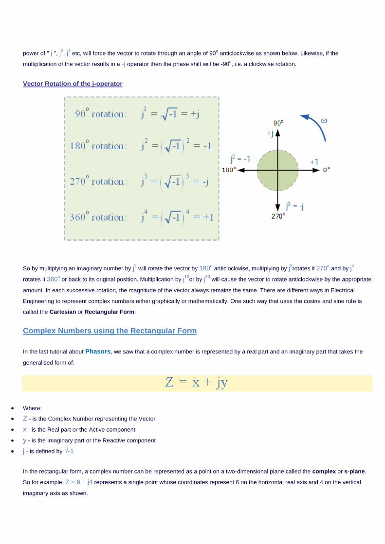
power of " j ", j2, j

3 etc, will force the vector to rotate through an angle of 90

o anticlockwise as shown below. Likewise, if the

multiplication of the vector results in a -j operator then the phase shift will be -90o, i.e. a clockwise rotation.

Vector Rotation of the j-operator

So by multiplying an imaginary number by j2 will rotate the vector by 180

o anticlockwise, multiplying by j

3rotates it 270

o and by j

4

rotates it 360o or back to its original position. Multiplication by j

10or by j

30 will cause the vector to rotate anticlockwise by the appropriate

amount. In each successive rotation, the magnitude of the vector always remains the same. There are different ways in Electrical

Engineering to represent complex numbers either graphically or mathematically. One such way that uses the cosine and sine rule is

called the Cartesian or Rectangular Form.

Complex Numbers using the Rectangular Form

In the last tutorial about Phasors, we saw that a complex number is represented by a real part and an imaginary part that takes the

generalised form of:

Where:

Z - is the Complex Number representing the Vector

x - is the Real part or the Active component

y - is the Imaginary part or the Reactive component

j - is defined by √-1

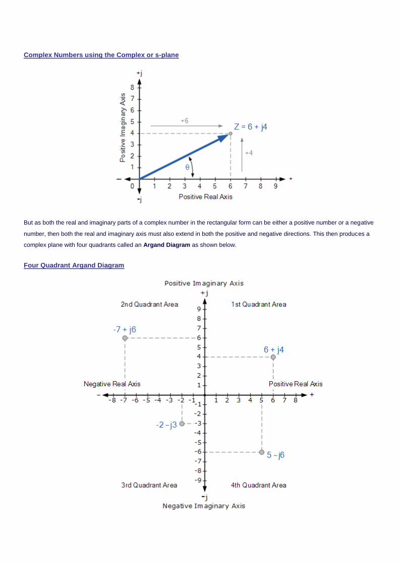
In the rectangular form, a complex number can be represented as a point on a two-dimensional plane called the complex or s-plane.

So for example, Z = 6 + j4 represents a single point whose coordinates represent 6 on the horizontal real axis and 4 on the vertical

imaginary axis as shown.

Complex Numbers using the Complex or s-plane

But as both the real and imaginary parts of a complex number in the rectangular form can be either a positive number or a negative

number, then both the real and imaginary axis must also extend in both the positive and negative directions. This then produces a

complex plane with four quadrants called an Argand Diagram as shown below.

Four Quadrant Argand Diagram

On the Argand diagram, the horizontal axis represents all positive real numbers to the right of the vertical imaginary axis and all

negative real numbers to the left of the vertical imaginary axis. All positive imaginary numbers are represented above the horizontal

axis while all the negative imaginary numbers are below the horizontal real axis. This then produces a two dimensional complex plane

with four distinct quadrants labelled, QI, QII, QIII, andQIV. The Argand diagram can also be used to represent a rotating phasor as a

point in the complex plane whose radius is given by the magnitude of the phasor will draw a full circle around it for every 2π/ω

seconds.

Complex Numbers can also have "zero" real or imaginary parts such as:Z = 6 + j0 or Z = 0 + j4. In this case the points are plotted

directly onto the real or imaginary axis. Also, the angle of a complex number can be calculated using simple trigonometry to calculate

the angles of right-angled triangles, or measured anti-clockwise around the Argand diagram starting from the positive real axis.

Then angles between 0 and 90o will be in the first quadrant ( I ), angles ( θ ) between 90 and 180

o in the second quadrant ( II ). The

third quadrant ( III ) includes angles between 180 and 270o while the fourth and final quadrant ( IV ) which completes the full circle

includes the angles between 270 and 360o and so on. In all the four quadrants the relevant angles can be found from tan

-1(imaginary

component/real component).

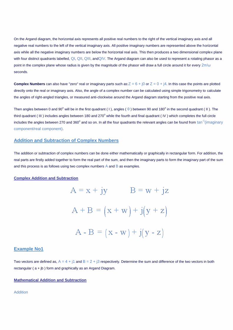
Addition and Subtraction of Complex Numbers

The addition or subtraction of complex numbers can be done either mathematically or graphically in rectangular form. For addition, the

real parts are firstly added together to form the real part of the sum, and then the imaginary parts to form the imaginary part of the sum

and this process is as follows using two complex numbers A and B as examples.

Complex Addition and Subtraction

Example No1

Two vectors are defined as, A = 4 + j1 and B = 2 + j3 respectively. Determine the sum and difference of the two vectors in both

rectangular ( a + jb ) form and graphically as an Argand Diagram.

Mathematical Addition and Subtraction

Addition

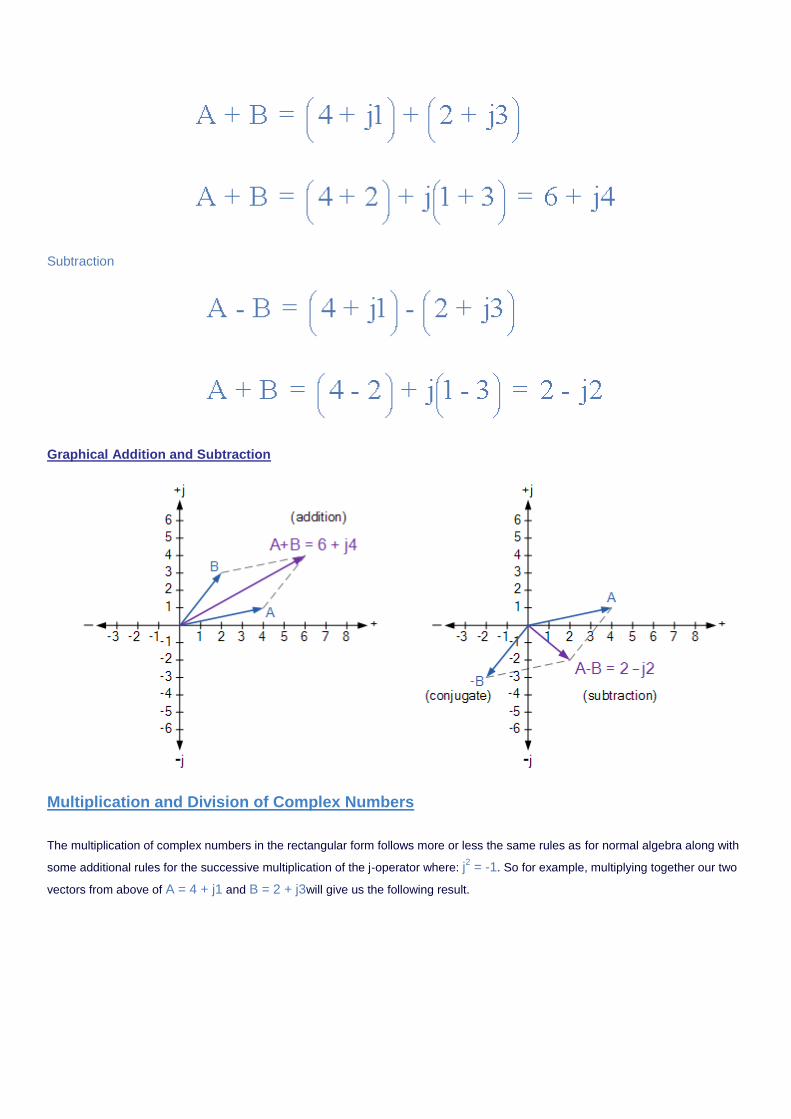
Subtraction

Graphical Addition and Subtraction

Multiplication and Division of Complex Numbers

The multiplication of complex numbers in the rectangular form follows more or less the same rules as for normal algebra along with

some additional rules for the successive multiplication of the j-operator where: j2 = -1. So for example, multiplying together our two

vectors from above of A = 4 + j1 and B = 2 + j3will give us the following result.

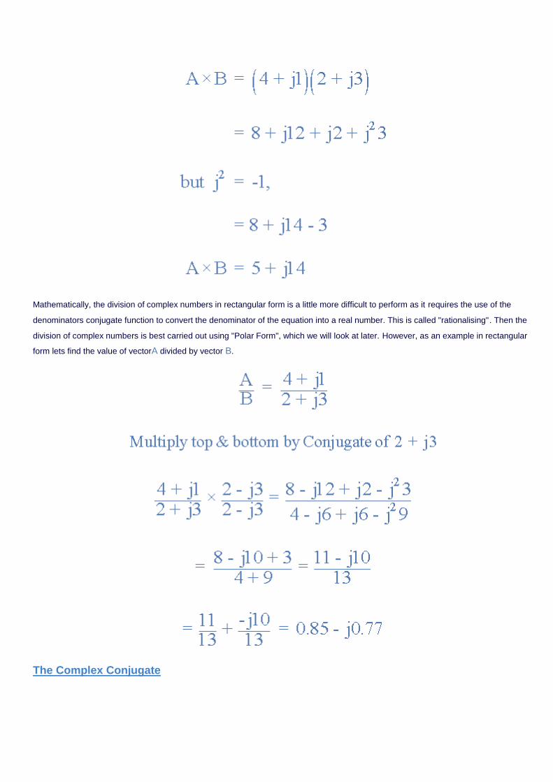
Mathematically, the division of complex numbers in rectangular form is a little more difficult to perform as it requires the use of the

denominators conjugate function to convert the denominator of the equation into a real number. This is called "rationalising". Then the

division of complex numbers is best carried out using "Polar Form", which we will look at later. However, as an example in rectangular

form lets find the value of vectorA divided by vector B.

The Complex Conjugate

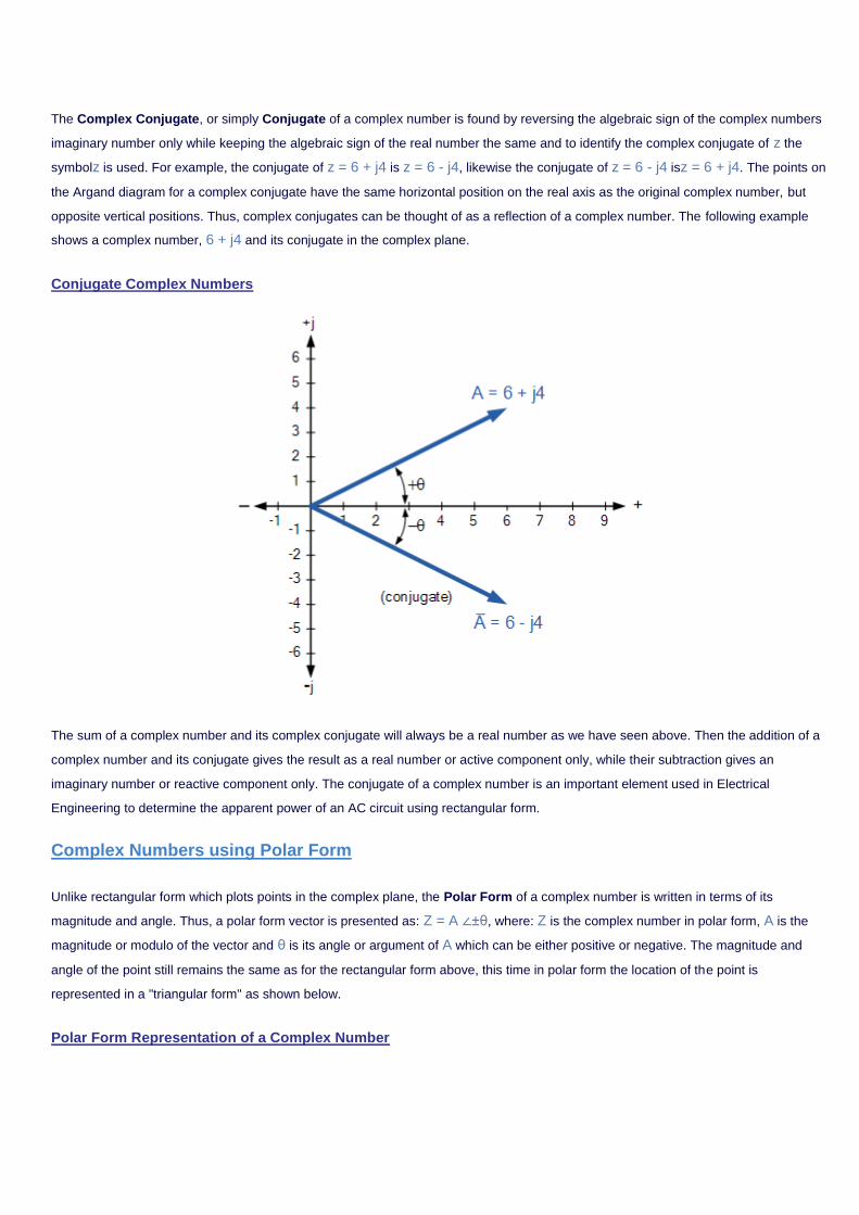
The Complex Conjugate, or simply Conjugate of a complex number is found by reversing the algebraic sign of the complex numbers

imaginary number only while keeping the algebraic sign of the real number the same and to identify the complex conjugate of z the

symbolz is used. For example, the conjugate of z = 6 + j4 is z = 6 - j4, likewise the conjugate of z = 6 - j4 isz = 6 + j4. The points on

the Argand diagram for a complex conjugate have the same horizontal position on the real axis as the original complex number, but

opposite vertical positions. Thus, complex conjugates can be thought of as a reflection of a complex number. The following example

shows a complex number, 6 + j4 and its conjugate in the complex plane.

Conjugate Complex Numbers

The sum of a complex number and its complex conjugate will always be a real number as we have seen above. Then the addition of a

complex number and its conjugate gives the result as a real number or active component only, while their subtraction gives an

imaginary number or reactive component only. The conjugate of a complex number is an important element used in Electrical

Engineering to determine the apparent power of an AC circuit using rectangular form.

Complex Numbers using Polar Form

Unlike rectangular form which plots points in the complex plane, the Polar Form of a complex number is written in terms of its

magnitude and angle. Thus, a polar form vector is presented as: Z = A ∠±θ, where: Z is the complex number in polar form, A is the

magnitude or modulo of the vector and θ is its angle or argument of A which can be either positive or negative. The magnitude and

angle of the point still remains the same as for the rectangular form above, this time in polar form the location of the point is

represented in a "triangular form" as shown below.

Polar Form Representation of a Complex Number

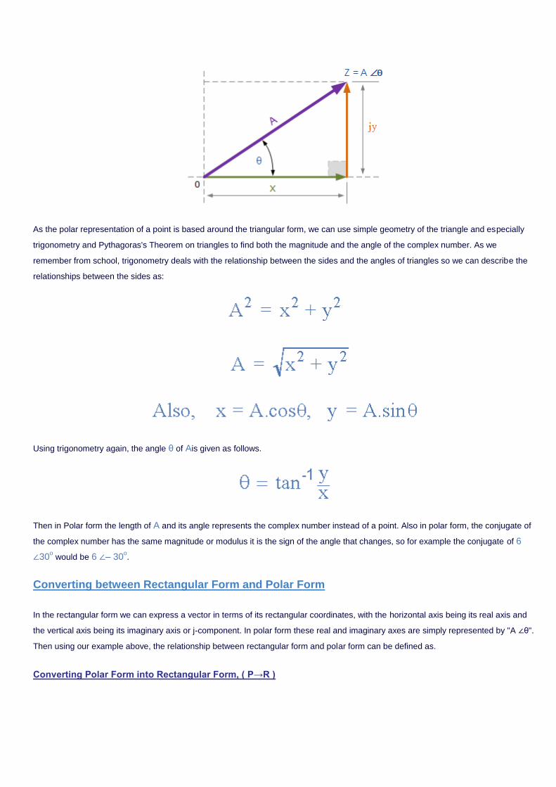
As the polar representation of a point is based around the triangular form, we can use simple geometry of the triangle and especially

trigonometry and Pythagoras's Theorem on triangles to find both the magnitude and the angle of the complex number. As we

remember from school, trigonometry deals with the relationship between the sides and the angles of triangles so we can describe the

relationships between the sides as:

Using trigonometry again, the angle θ of Ais given as follows.

Then in Polar form the length of A and its angle represents the complex number instead of a point. Also in polar form, the conjugate of

the complex number has the same magnitude or modulus it is the sign of the angle that changes, so for example the conjugate of 6

∠30o would be 6 ∠– 30

o.

Converting between Rectangular Form and Polar Form

In the rectangular form we can express a vector in terms of its rectangular coordinates, with the horizontal axis being its real axis and

the vertical axis being its imaginary axis or j-component. In polar form these real and imaginary axes are simply represented by "A ∠θ".

Then using our example above, the relationship between rectangular form and polar form can be defined as.

Converting Polar Form into Rectangular Form, ( P→R )

We can also convert back from rectangular form to polar form as follows.

Converting Rectangular Form into Polar Form, ( R→P )

Polar Form Multiplication and Division

Rectangular form is best for adding and subtracting complex numbers as we saw above, but polar form is often better for multiplying

and dividing. To multiply together two vectors in polar form, we must first multiply together the two modulus or magnitudes and then

add together their angles.

Multiplication in Polar Form

Multiplying together 6 ∠30o and8 ∠– 45

o in polar form gives us.

Division in Polar Form

Likewise, to divide together two vectors in polar form, we must divide the two modulus and then subtract their angles as shown.

Fortunately todays modern scientific calculators have built in mathematical functions that allow for the easy conversion of rectangular to

polar form, ( R → P ) or polar to rectangular form, ( R → P ).

Complex Numbers using Exponential Form

So far we have considered complex numbers in the Rectangular Form, ( a + jb ) and the Polar Form, ( A ∠±θ ).But there is also a

third method for representing a complex number which is similar to the polar form that corresponds to the length (magnitude) and

phase angle of the sinusoid but uses the base of the natural logarithm,e = 2.718 281.. to find the value of the complex number. This

third method is called the Exponential Form.

The Exponential Form uses the trigonometric functions of both the sine ( sin ) and the cosine ( cos ) values of a right angled triangle

to define the complex exponential as a rotating point in the complex plane. The exponential form for finding the position of the point is

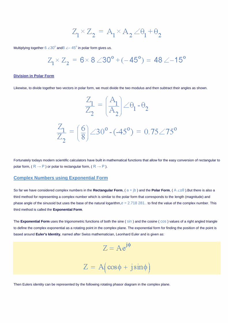
based around Euler's Identity, named after Swiss mathematician, Leonhard Euler and is given as:

Then Eulers identity can be represented by the following rotating phasor diagram in the complex plane.

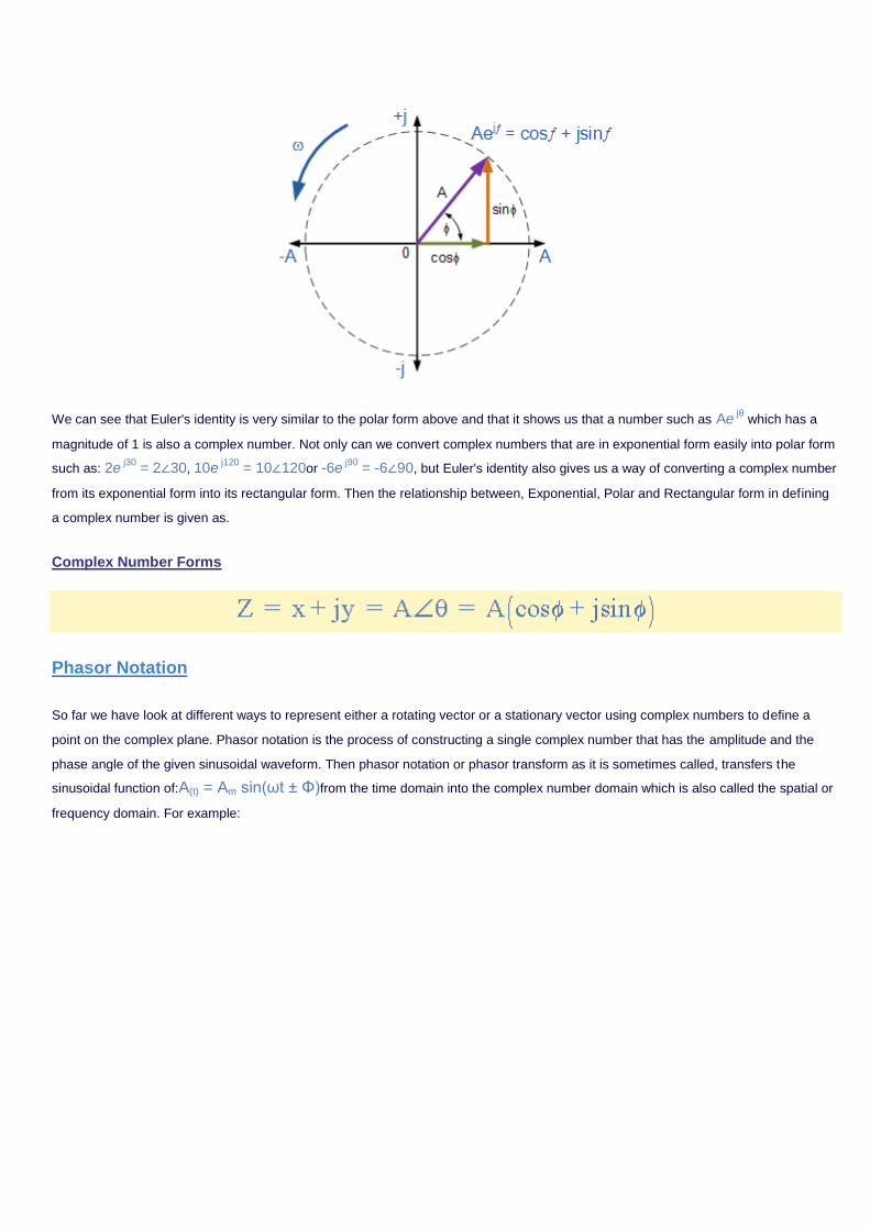
We can see that Euler's identity is very similar to the polar form above and that it shows us that a number such as Ae jθ

which has a

magnitude of 1 is also a complex number. Not only can we convert complex numbers that are in exponential form easily into polar form

such as: 2e j30

= 2∠30, 10e j120

= 10∠120or -6e j90

= -6∠90, but Euler's identity also gives us a way of converting a complex number

from its exponential form into its rectangular form. Then the relationship between, Exponential, Polar and Rectangular form in defining

a complex number is given as.

Complex Number Forms

Phasor Notation

So far we have look at different ways to represent either a rotating vector or a stationary vector using complex numbers to define a

point on the complex plane. Phasor notation is the process of constructing a single complex number that has the amplitude and the

phase angle of the given sinusoidal waveform. Then phasor notation or phasor transform as it is sometimes called, transfers the

sinusoidal function of:A(t) = Am sin(ωt ± Φ)from the time domain into the complex number domain which is also called the spatial or

frequency domain. For example:

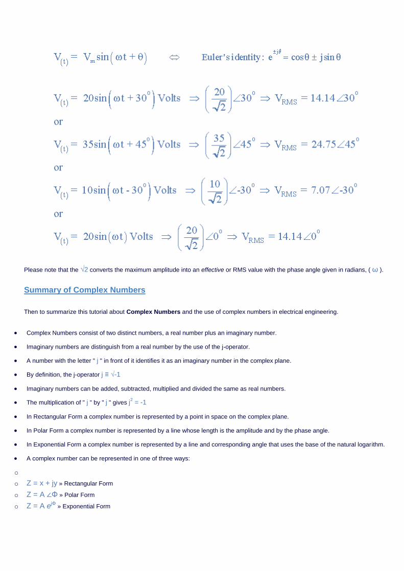
Please note that the √2 converts the maximum amplitude into an effective or RMS value with the phase angle given in radians, ( ω ).

Summary of Complex Numbers

Then to summarize this tutorial about Complex Numbers and the use of complex numbers in electrical engineering.

Complex Numbers consist of two distinct numbers, a real number plus an imaginary number.

Imaginary numbers are distinguish from a real number by the use of the j-operator.

A number with the letter " j " in front of it identifies it as an imaginary number in the complex plane.

By definition, the j-operator j ≡ √-1

Imaginary numbers can be added, subtracted, multiplied and divided the same as real numbers.

The multiplication of " j " by " j " gives j2 = -1

In Rectangular Form a complex number is represented by a point in space on the complex plane.

In Polar Form a complex number is represented by a line whose length is the amplitude and by the phase angle.

In Exponential Form a complex number is represented by a line and corresponding angle that uses the base of the natural logarithm.

A complex number can be represented in one of three ways:

o

o Z = x + jy » Rectangular Form

o Z = A ∠Φ » Polar Form

o Z = A ejΦ » Exponential Form

Euler's identity can be used to convert Complex Numbers from exponential form into rectangular form.

In the previous tutorials including this one we have seen that we can use phasors to represent sinusoidal waveforms and that their

amplitude and phase angle can be written in the form of a complex number. We have also seen thatComplex Numbers can be

presented in rectangular, polar or exponential form with the conversion between each form including addition, subtracting, multiplication

and division.

In the next few tutorials relating to the phasor relationship in AC series circuits, we will look at the impedance of some common passive

circuit components and draw the phasor diagrams for both the current flowing through the component and the voltage applied across it

starting with theAC Resistance.

AC Resistance & Impedance Navigation

Tutorial: 6 of 12

--- Select a Tutorial Page ---

RESET

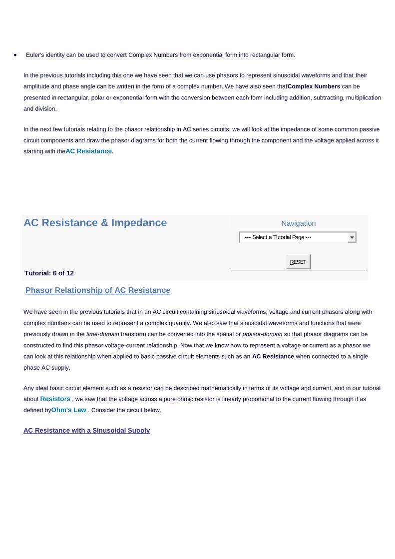
Phasor Relationship of AC Resistance

We have seen in the previous tutorials that in an AC circuit containing sinusoidal waveforms, voltage and current phasors along with

complex numbers can be used to represent a complex quantity. We also saw that sinusoidal waveforms and functions that were

previously drawn in the time-domain transform can be converted into the spatial or phasor-domain so that phasor diagrams can be

constructed to find this phasor voltage-current relationship. Now that we know how to represent a voltage or current as a phasor we

can look at this relationship when applied to basic passive circuit elements such as an AC Resistance when connected to a single

phase AC supply.

Any ideal basic circuit element such as a resistor can be described mathematically in terms of its voltage and current, and in our tutorial

about Resistors , we saw that the voltage across a pure ohmic resistor is linearly proportional to the current flowing through it as

defined byOhm's Law . Consider the circuit below.

AC Resistance with a Sinusoidal Supply

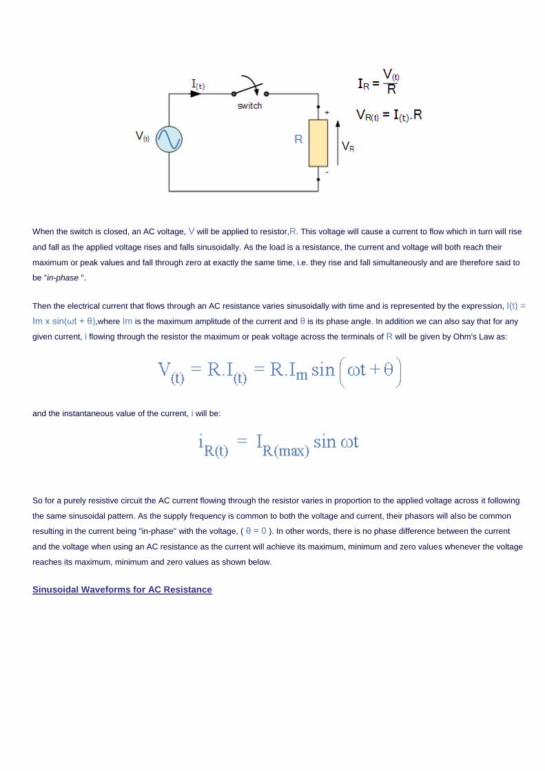
When the switch is closed, an AC voltage, V will be applied to resistor,R. This voltage will cause a current to flow which in turn will rise

and fall as the applied voltage rises and falls sinusoidally. As the load is a resistance, the current and voltage will both reach their

maximum or peak values and fall through zero at exactly the same time, i.e. they rise and fall simultaneously and are therefore said to

be "in-phase ".

Then the electrical current that flows through an AC resistance varies sinusoidally with time and is represented by the expression, I(t) =

Im x sin(ωt + θ),where Im is the maximum amplitude of the current and θ is its phase angle. In addition we can also say that for any

given current, i flowing through the resistor the maximum or peak voltage across the terminals of R will be given by Ohm's Law as:

and the instantaneous value of the current, i will be:

So for a purely resistive circuit the AC current flowing through the resistor varies in proportion to the applied voltage across it following

the same sinusoidal pattern. As the supply frequency is common to both the voltage and current, their phasors will also be common

resulting in the current being "in-phase" with the voltage, ( θ = 0 ). In other words, there is no phase difference between the current

and the voltage when using an AC resistance as the current will achieve its maximum, minimum and zero values whenever the voltage

reaches its maximum, minimum and zero values as shown below.

Sinusoidal Waveforms for AC Resistance

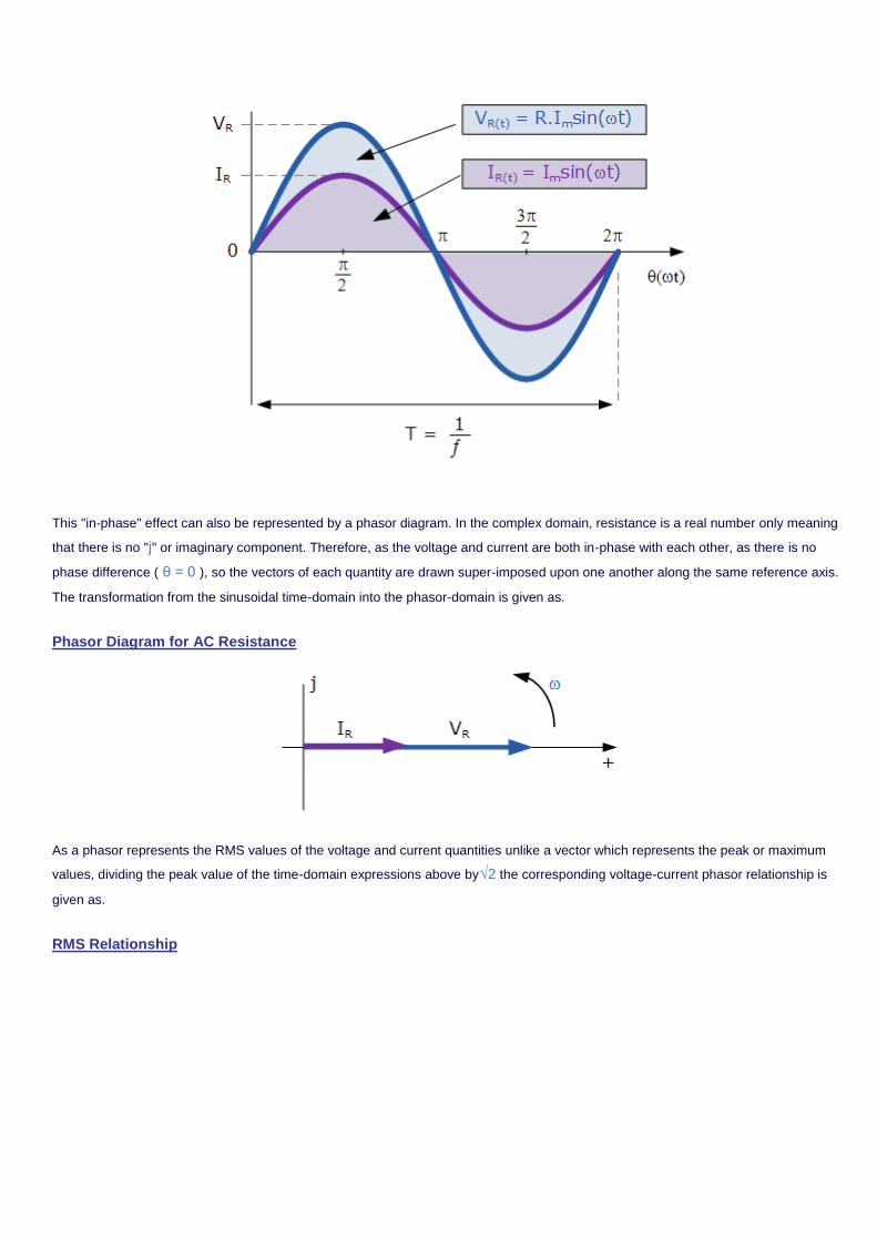
This "in-phase" effect can also be represented by a phasor diagram. In the complex domain, resistance is a real number only meaning

that there is no "j" or imaginary component. Therefore, as the voltage and current are both in-phase with each other, as there is no

phase difference ( θ = 0 ), so the vectors of each quantity are drawn super-imposed upon one another along the same reference axis.

The transformation from the sinusoidal time-domain into the phasor-domain is given as.

Phasor Diagram for AC Resistance

As a phasor represents the RMS values of the voltage and current quantities unlike a vector which represents the peak or maximum

values, dividing the peak value of the time-domain expressions above by√2 the corresponding voltage-current phasor relationship is

given as.

RMS Relationship

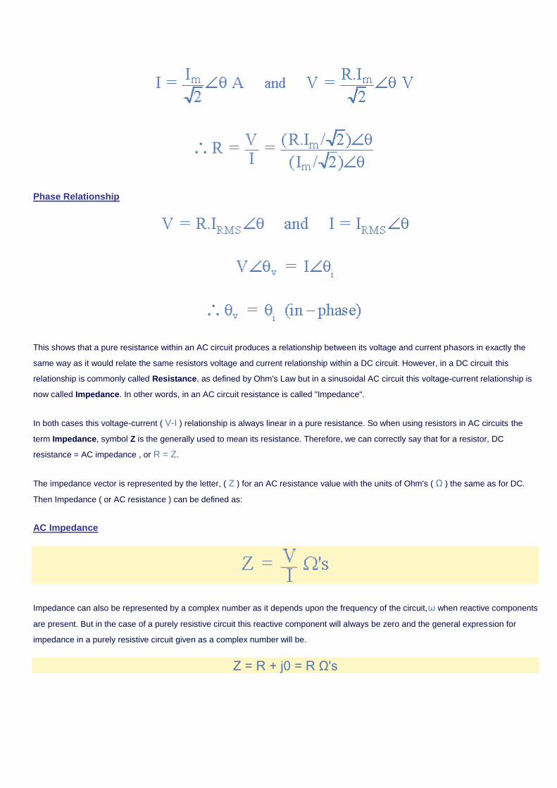
Phase Relationship

This shows that a pure resistance within an AC circuit produces a relationship between its voltage and current phasors in exactly the

same way as it would relate the same resistors voltage and current relationship within a DC circuit. However, in a DC circuit this

relationship is commonly called Resistance, as defined by Ohm's Law but in a sinusoidal AC circuit this voltage-current relationship is

now called Impedance. In other words, in an AC circuit resistance is called "Impedance".

In both cases this voltage-current ( V-I ) relationship is always linear in a pure resistance. So when using resistors in AC circuits the

term Impedance, symbol Z is the generally used to mean its resistance. Therefore, we can correctly say that for a resistor, DC

resistance = AC impedance , or R = Z.

The impedance vector is represented by the letter, ( Z ) for an AC resistance value with the units of Ohm's ( Ω ) the same as for DC.

Then Impedance ( or AC resistance ) can be defined as:

AC Impedance

Impedance can also be represented by a complex number as it depends upon the frequency of the circuit,ω when reactive components

are present. But in the case of a purely resistive circuit this reactive component will always be zero and the general expression for

impedance in a purely resistive circuit given as a complex number will be.

Z = R + j0 = R Ω's

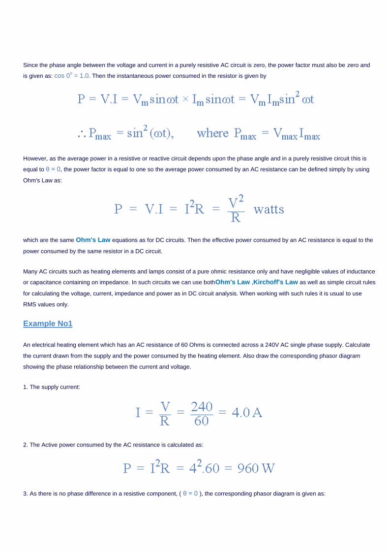
Since the phase angle between the voltage and current in a purely resistive AC circuit is zero, the power factor must also be zero and

is given as: cos 0o = 1.0. Then the instantaneous power consumed in the resistor is given by

However, as the average power in a resistive or reactive circuit depends upon the phase angle and in a purely resistive circuit this is

equal to θ = 0, the power factor is equal to one so the average power consumed by an AC resistance can be defined simply by using

Ohm's Law as:

which are the same Ohm's Law equations as for DC circuits. Then the effective power consumed by an AC resistance is equal to the

power consumed by the same resistor in a DC circuit.

Many AC circuits such as heating elements and lamps consist of a pure ohmic resistance only and have negligible values of inductance

or capacitance containing on impedance. In such circuits we can use bothOhm's Law ,Kirchoff's Law as well as simple circuit rules

for calculating the voltage, current, impedance and power as in DC circuit analysis. When working with such rules it is usual to use

RMS values only.

Example No1

An electrical heating element which has an AC resistance of 60 Ohms is connected across a 240V AC single phase supply. Calculate

the current drawn from the supply and the power consumed by the heating element. Also draw the corresponding phasor diagram

showing the phase relationship between the current and voltage.

1. The supply current:

2. The Active power consumed by the AC resistance is calculated as:

3. As there is no phase difference in a resistive component, ( θ = 0 ), the corresponding phasor diagram is given as:

Example No2

A sinusoidal voltage supply defined as:V(t) = 100 x cos(ωt + 30o) is connected to a pure resistance of 50 Ohms. Determine its

impedance and the value of the current flowing through the circuit. Draw the corresponding phasor diagram.

The sinusoidal voltage across the resistance will be the same as for the supply in a purely resistive circuit. Converting this voltage from

the time-domain expression into the phasor-domain expression gives us:

Applying Ohms Law gives us:

The corresponding phasor diagram will therefore be:

Impedance Summary

In a pure ohmic AC Resistance, the current and voltage are both "in-phase" as there is no phase difference between them. The

current flowing through the resistance is directly proportional to the voltage across it with this linear relationship in an AC circuit being

called Impedance. Impedance, which is given the letter Z, in a pure ohmic resistance is a complex number consisting only of a real

part being the actual AC resistance value, ( R ) and a zero imaginary part, ( j0 ). Because of this Ohm's Law can be used in circuits

containing an AC resistance to calculate these voltages and currents.

In the next tutorial about AC Inductancewe will look at the voltage-current relationship of an inductor when a steady state sinusoidal

AC waveform is applied to it along with its phasor diagram representation for both pure and non-pure inductances.

AC Inductance & Inductive Reactance Navigation

Tutorial: 7 of 12

--- Select a Tutorial Page ---

RESET

AC Inductance

We know from the tutorials aboutInductors, that inductors are basically coils or loops of wire that are either wound around a hollow

tube former (air cored) or wound around some ferromagnetic material (iron cored) to increase their inductive value called inductance.

Inductors store their energy in the form of a magnetic field that is created when a DC voltage is applied across the terminals of an

inductor. The growth of the current flowing through the inductor is not instant but is determined by the inductors own self-induced or

back emf value. Then for an inductor coil, this back emf voltage VL is proportional to the rate of change of the current flowing through it.

This current will continue to rise until it reaches its maximum steady state condition which is around five time constants when this self-

induced back emf has decayed to zero. At this point a steady state DC current is flowing through the coil, no more back emf is induced

to oppose the current flow and therefore, the coil acts more like a short circuit allowing maximum current to flow through it.

However, in an alternating current circuit which contains an AC Inductance, the flow of current through an inductor behaves very

differently to that of a steady state DC voltage. Now in an AC circuit, the opposition to the current flowing through the coils windings not

only depends upon the inductance of the coil but also the frequency of the applied voltage waveform as it varies from its positive to

negative values.

The actual opposition to the current flowing through a coil in an AC circuit is determined by theAC Resistance of the coil with this AC

resistance being represented by a complex number. But to distinguish a DC resistance value from an AC resistance value, which is

also known as Impedance, the term Reactance is used. Like resistance, reactance is measured in Ohm's but is given the symbol Xto

distinguish it from a purely resistive R value and as the component in question is an inductor, the reactance of an inductor is called

Inductive Reactance, ( XL ) and is measured in Ohms. Its value can be found from the formula.

Inductive Reactance

Where: XL is the Inductive Reactance in Ohms, ƒ is the frequency in Hertz and L is the inductance of the coil in Henries.

We can also define inductive reactance in radians, where Omega, ω equals 2πƒ.

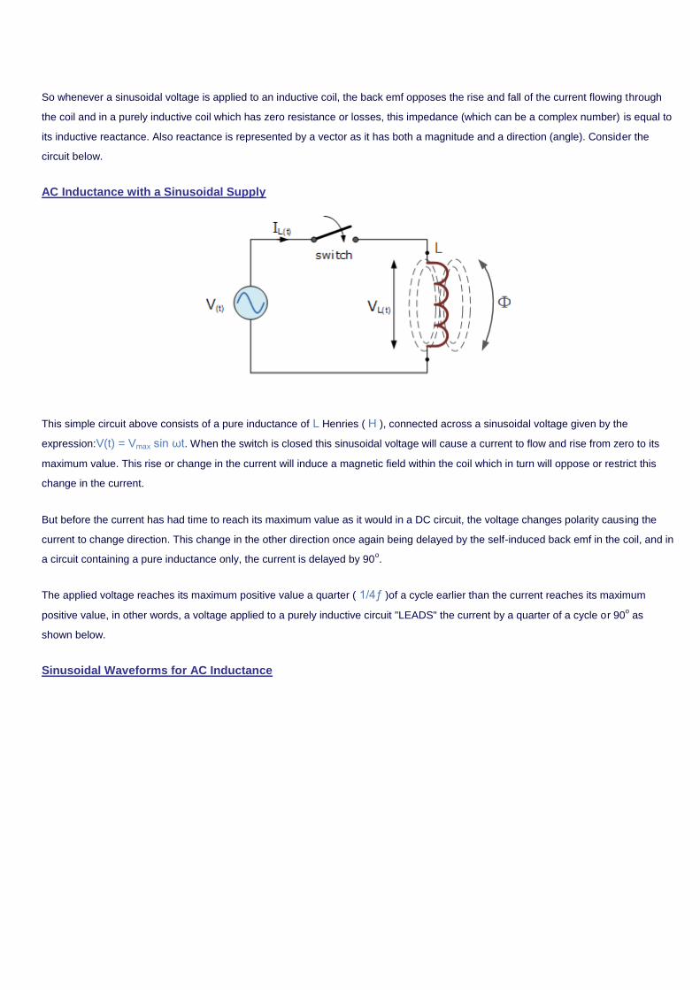
So whenever a sinusoidal voltage is applied to an inductive coil, the back emf opposes the rise and fall of the current flowing through

the coil and in a purely inductive coil which has zero resistance or losses, this impedance (which can be a complex number) is equal to

its inductive reactance. Also reactance is represented by a vector as it has both a magnitude and a direction (angle). Consider the

circuit below.

AC Inductance with a Sinusoidal Supply

This simple circuit above consists of a pure inductance of L Henries ( H ), connected across a sinusoidal voltage given by the

expression:V(t) = Vmax sin ωt. When the switch is closed this sinusoidal voltage will cause a current to flow and rise from zero to its

maximum value. This rise or change in the current will induce a magnetic field within the coil which in turn will oppose or restrict this

change in the current.

But before the current has had time to reach its maximum value as it would in a DC circuit, the voltage changes polarity causing the

current to change direction. This change in the other direction once again being delayed by the self-induced back emf in the coil, and in

a circuit containing a pure inductance only, the current is delayed by 90o.

The applied voltage reaches its maximum positive value a quarter ( 1/4ƒ )of a cycle earlier than the current reaches its maximum

positive value, in other words, a voltage applied to a purely inductive circuit "LEADS" the current by a quarter of a cycle or 90o as

shown below.

Sinusoidal Waveforms for AC Inductance

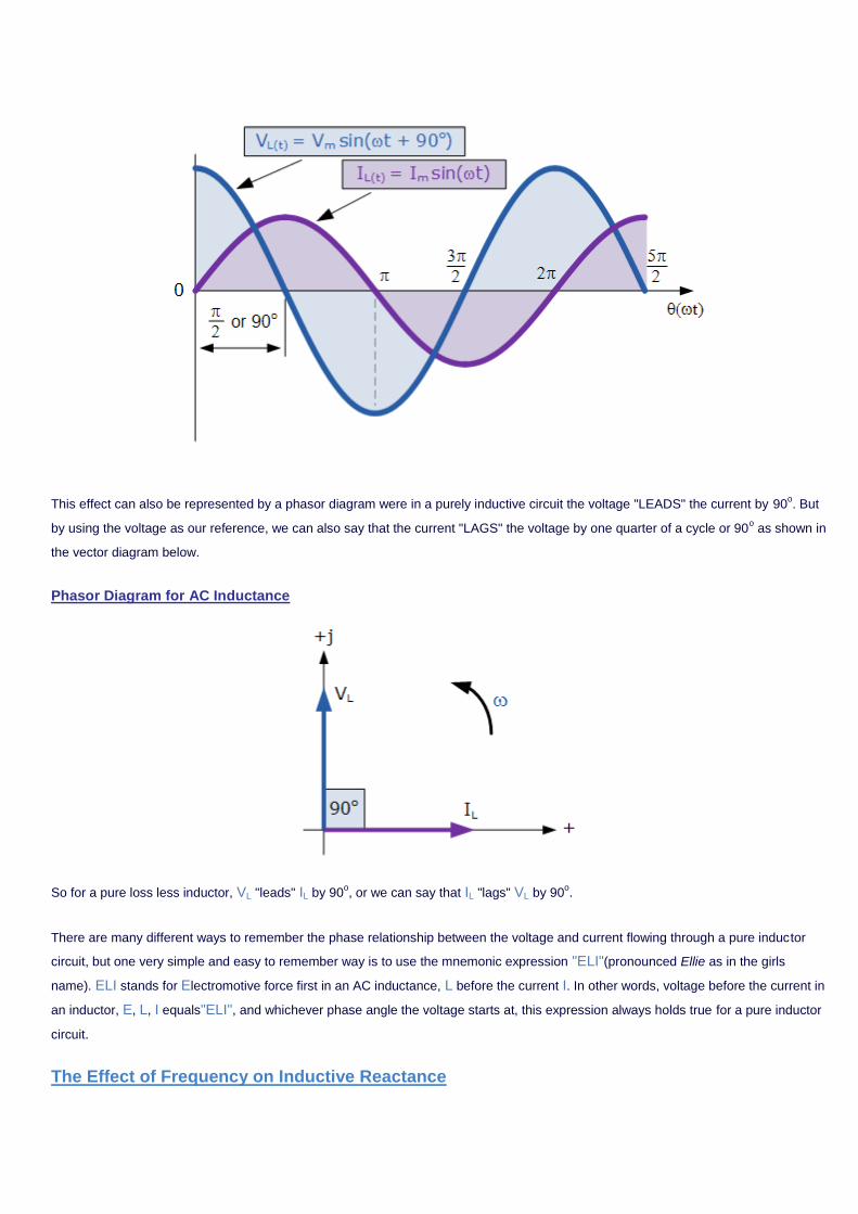
This effect can also be represented by a phasor diagram were in a purely inductive circuit the voltage "LEADS" the current by 90o. But

by using the voltage as our reference, we can also say that the current "LAGS" the voltage by one quarter of a cycle or 90o as shown in

the vector diagram below.

Phasor Diagram for AC Inductance

So for a pure loss less inductor, VL "leads" IL by 90o, or we can say that IL "lags" VL by 90

o.

There are many different ways to remember the phase relationship between the voltage and current flowing through a pure inductor

circuit, but one very simple and easy to remember way is to use the mnemonic expression "ELI"(pronounced Ellie as in the girls

name). ELI stands for Electromotive force first in an AC inductance, L before the current I. In other words, voltage before the current in

an inductor, E, L, I equals"ELI", and whichever phase angle the voltage starts at, this expression always holds true for a pure inductor

circuit.

The Effect of Frequency on Inductive Reactance

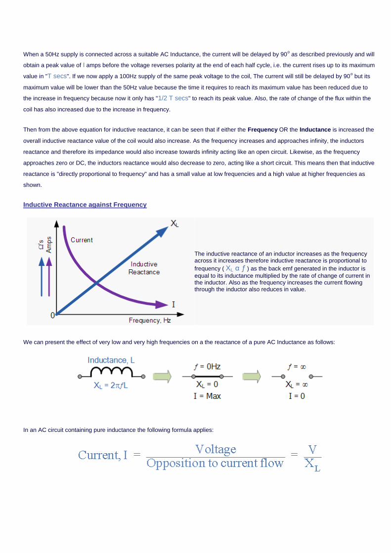
When a 50Hz supply is connected across a suitable AC Inductance, the current will be delayed by 90o as described previously and will

obtain a peak value of I amps before the voltage reverses polarity at the end of each half cycle, i.e. the current rises up to its maximum

value in "T secs". If we now apply a 100Hz supply of the same peak voltage to the coil, The current will still be delayed by 90o but its

maximum value will be lower than the 50Hz value because the time it requires to reach its maximum value has been reduced due to

the increase in frequency because now it only has "1/2 T secs" to reach its peak value. Also, the rate of change of the flux within the

coil has also increased due to the increase in frequency.

Then from the above equation for inductive reactance, it can be seen that if either the Frequency OR the Inductance is increased the

overall inductive reactance value of the coil would also increase. As the frequency increases and approaches infinity, the inductors

reactance and therefore its impedance would also increase towards infinity acting like an open circuit. Likewise, as the frequency

approaches zero or DC, the inductors reactance would also decrease to zero, acting like a short circuit. This means then that inductive

reactance is "directly proportional to frequency" and has a small value at low frequencies and a high value at higher frequencies as

shown.

Inductive Reactance against Frequency

The inductive reactance of an inductor increases as the frequency across it increases therefore inductive reactance is proportional to

frequency ( XL α ƒ ) as the back emf generated in the inductor is

equal to its inductance multiplied by the rate of change of current in the inductor. Also as the frequency increases the current flowing through the inductor also reduces in value.

We can present the effect of very low and very high frequencies on a the reactance of a pure AC Inductance as follows:

In an AC circuit containing pure inductance the following formula applies:

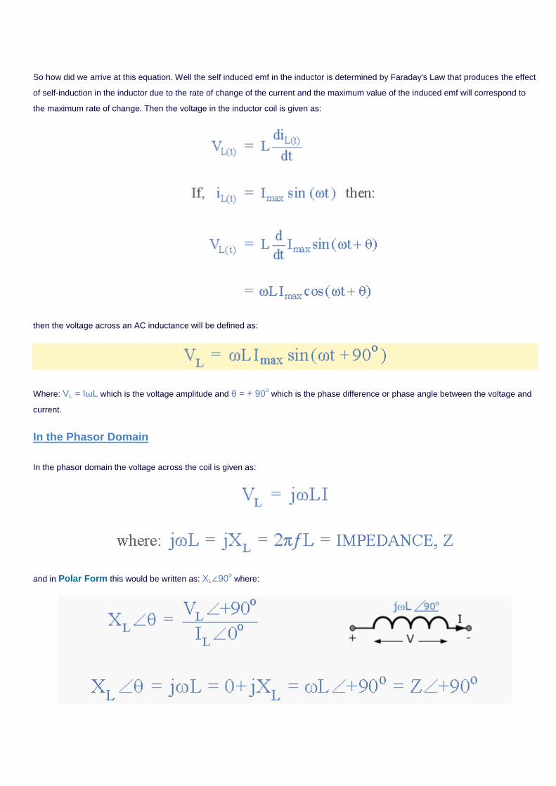
So how did we arrive at this equation. Well the self induced emf in the inductor is determined by Faraday's Law that produces the effect

of self-induction in the inductor due to the rate of change of the current and the maximum value of the induced emf will correspond to

the maximum rate of change. Then the voltage in the inductor coil is given as:

then the voltage across an AC inductance will be defined as:

Where: VL = IωL which is the voltage amplitude and θ = + 90o which is the phase difference or phase angle between the voltage and

current.

In the Phasor Domain

In the phasor domain the voltage across the coil is given as:

and in Polar Form this would be written as: XL∠90o where:

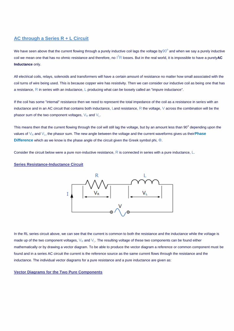
AC through a Series R + L Circuit

We have seen above that the current flowing through a purely inductive coil lags the voltage by90o and when we say a purely inductive

coil we mean one that has no ohmic resistance and therefore, no I2R losses. But in the real world, it is impossible to have a purelyAC

Inductance only.

All electrical coils, relays, solenoids and transformers will have a certain amount of resistance no matter how small associated with the

coil turns of wire being used. This is because copper wire has resistivity. Then we can consider our inductive coil as being one that has

a resistance, R in series with an inductance, L producing what can be loosely called an "impure inductance".

If the coil has some "internal" resistance then we need to represent the total impedance of the coil as a resistance in series with an

inductance and in an AC circuit that contains both inductance, Land resistance, R the voltage, V across the combination will be the

phasor sum of the two component voltages, VR and VL.

This means then that the current flowing through the coil will still lag the voltage, but by an amount less than 90o depending upon the

values of VR and VL, the phasor sum. The new angle between the voltage and the current waveforms gives us theirPhase

Difference which as we know is the phase angle of the circuit given the Greek symbol phi, Φ.

Consider the circuit below were a pure non-inductive resistance, R is connected in series with a pure inductance, L.

Series Resistance-Inductance Circuit

In the RL series circuit above, we can see that the current is common to both the resistance and the inductance while the voltage is

made up of the two component voltages, VR and VL. The resulting voltage of these two components can be found either

mathematically or by drawing a vector diagram. To be able to produce the vector diagram a reference or common component must be

found and in a series AC circuit the current is the reference source as the same current flows through the resistance and the

inductance. The individual vector diagrams for a pure resistance and a pure inductance are given as:

Vector Diagrams for the Two Pure Components

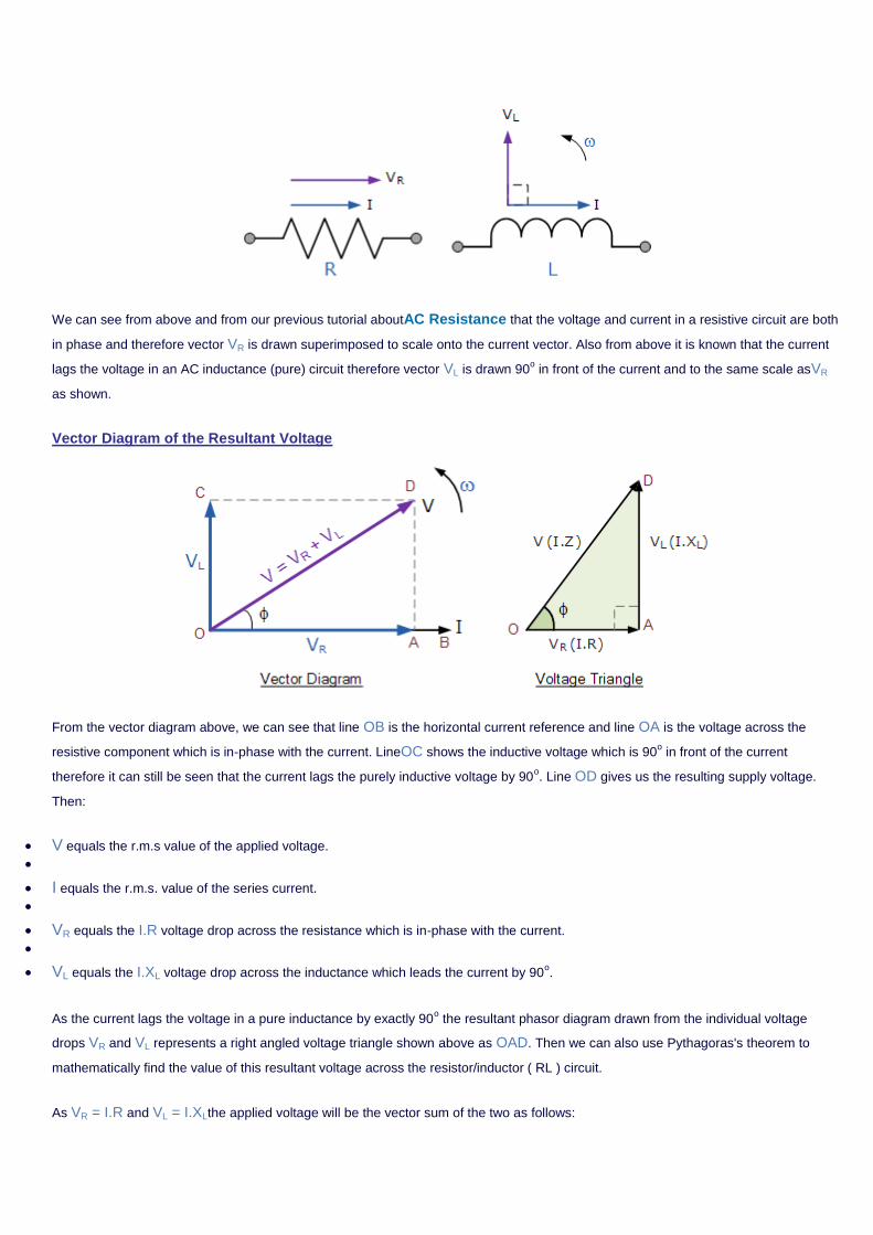
We can see from above and from our previous tutorial aboutAC Resistance that the voltage and current in a resistive circuit are both

in phase and therefore vector VR is drawn superimposed to scale onto the current vector. Also from above it is known that the current

lags the voltage in an AC inductance (pure) circuit therefore vector VL is drawn 90o in front of the current and to the same scale asVR

as shown.

Vector Diagram of the Resultant Voltage

From the vector diagram above, we can see that line OB is the horizontal current reference and line OA is the voltage across the

resistive component which is in-phase with the current. LineOC shows the inductive voltage which is 90o in front of the current

therefore it can still be seen that the current lags the purely inductive voltage by 90o. Line OD gives us the resulting supply voltage.

Then:

V equals the r.m.s value of the applied voltage.

I equals the r.m.s. value of the series current.

VR equals the I.R voltage drop across the resistance which is in-phase with the current.

VL equals the I.XL voltage drop across the inductance which leads the current by 90o.

As the current lags the voltage in a pure inductance by exactly 90o the resultant phasor diagram drawn from the individual voltage

drops VR and VL represents a right angled voltage triangle shown above as OAD. Then we can also use Pythagoras's theorem to

mathematically find the value of this resultant voltage across the resistor/inductor ( RL ) circuit.

As VR = I.R and VL = I.XLthe applied voltage will be the vector sum of the two as follows:

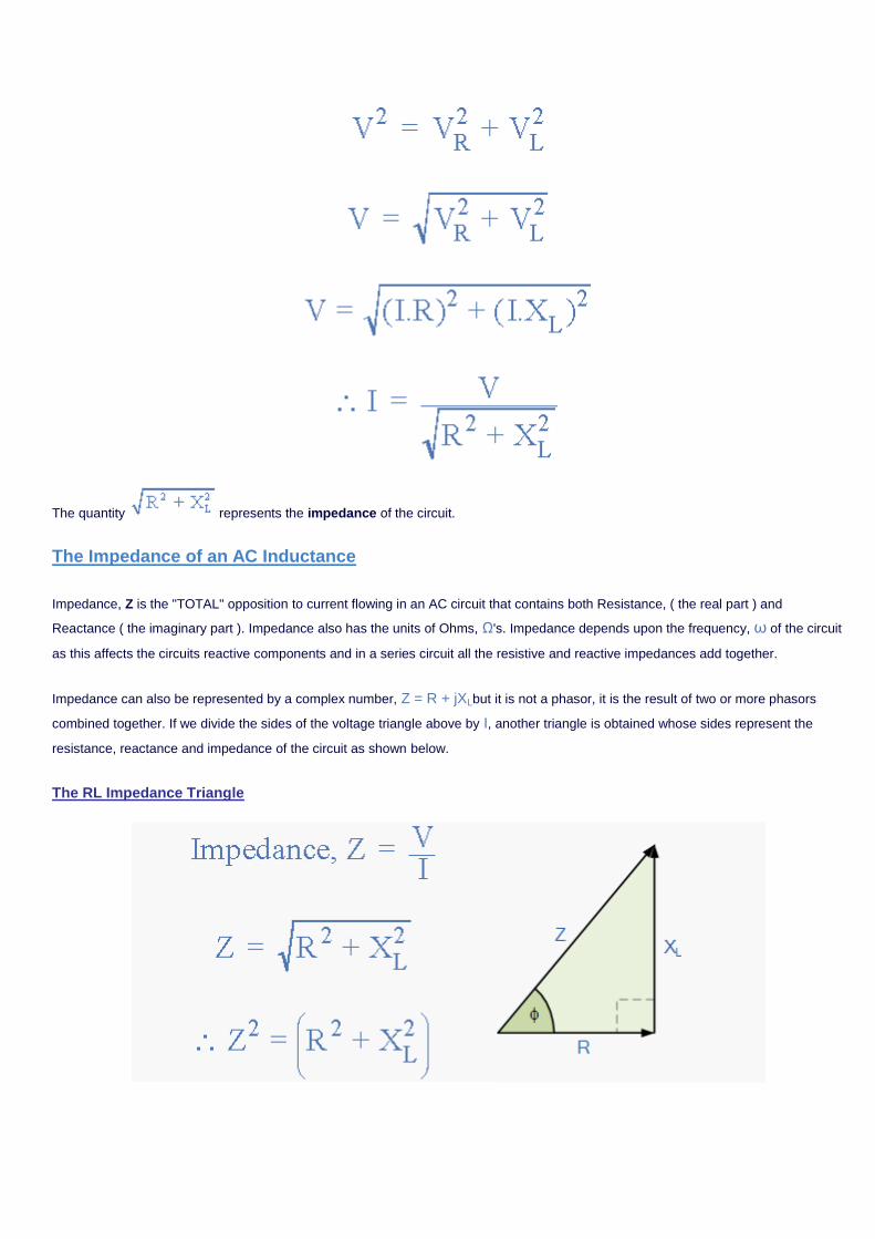
The quantity represents the impedance of the circuit.

The Impedance of an AC Inductance

Impedance, Z is the "TOTAL" opposition to current flowing in an AC circuit that contains both Resistance, ( the real part ) and

Reactance ( the imaginary part ). Impedance also has the units of Ohms, Ω's. Impedance depends upon the frequency, ω of the circuit

as this affects the circuits reactive components and in a series circuit all the resistive and reactive impedances add together.

Impedance can also be represented by a complex number, Z = R + jXLbut it is not a phasor, it is the result of two or more phasors

combined together. If we divide the sides of the voltage triangle above by I, another triangle is obtained whose sides represent the

resistance, reactance and impedance of the circuit as shown below.

The RL Impedance Triangle

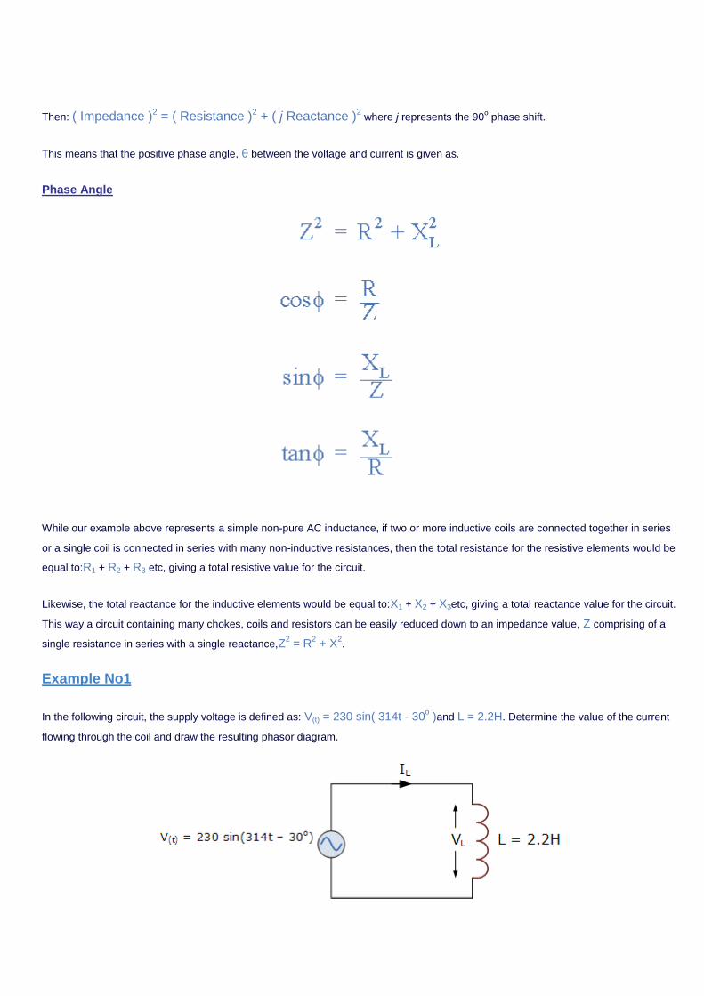
Then: ( Impedance )2 = ( Resistance )2 + ( j Reactance )2 where j represents the 90

o phase shift.

This means that the positive phase angle, θ between the voltage and current is given as.

Phase Angle

While our example above represents a simple non-pure AC inductance, if two or more inductive coils are connected together in series

or a single coil is connected in series with many non-inductive resistances, then the total resistance for the resistive elements would be

equal to:R1 + R2 + R3 etc, giving a total resistive value for the circuit.

Likewise, the total reactance for the inductive elements would be equal to:X1 + X2 + X3etc, giving a total reactance value for the circuit.

This way a circuit containing many chokes, coils and resistors can be easily reduced down to an impedance value, Z comprising of a

single resistance in series with a single reactance,Z2 = R

2 + X

2.

Example No1

In the following circuit, the supply voltage is defined as: V(t) = 230 sin( 314t - 30o )and L = 2.2H. Determine the value of the current

flowing through the coil and draw the resulting phasor diagram.

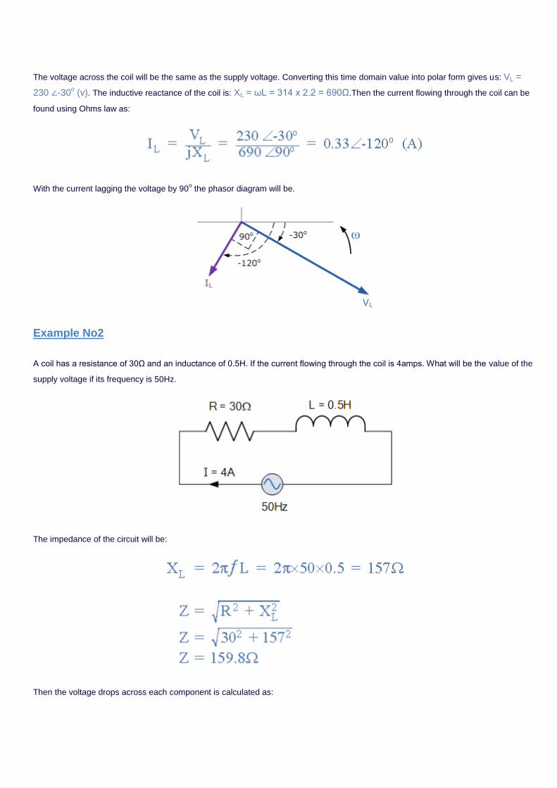
The voltage across the coil will be the same as the supply voltage. Converting this time domain value into polar form gives us: VL =

230 ∠-30o (v). The inductive reactance of the coil is: XL = ωL = 314 x 2.2 = 690Ω.Then the current flowing through the coil can be

found using Ohms law as:

With the current lagging the voltage by 90o the phasor diagram will be.

Example No2

A coil has a resistance of 30Ω and an inductance of 0.5H. If the current flowing through the coil is 4amps. What will be the value of the

supply voltage if its frequency is 50Hz.

The impedance of the circuit will be:

Then the voltage drops across each component is calculated as:

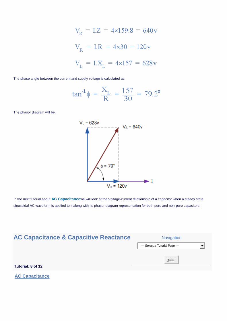
The phase angle between the current and supply voltage is calculated as:

The phasor diagram will be.

In the next tutorial about AC Capacitancewe will look at the Voltage-current relationship of a capacitor when a steady state

sinusoidal AC waveform is applied to it along with its phasor diagram representation for both pure and non-pure capacitors.

AC Capacitance & Capacitive Reactance Navigation

Tutorial: 8 of 12

--- Select a Tutorial Page ---

RESET

AC Capacitance

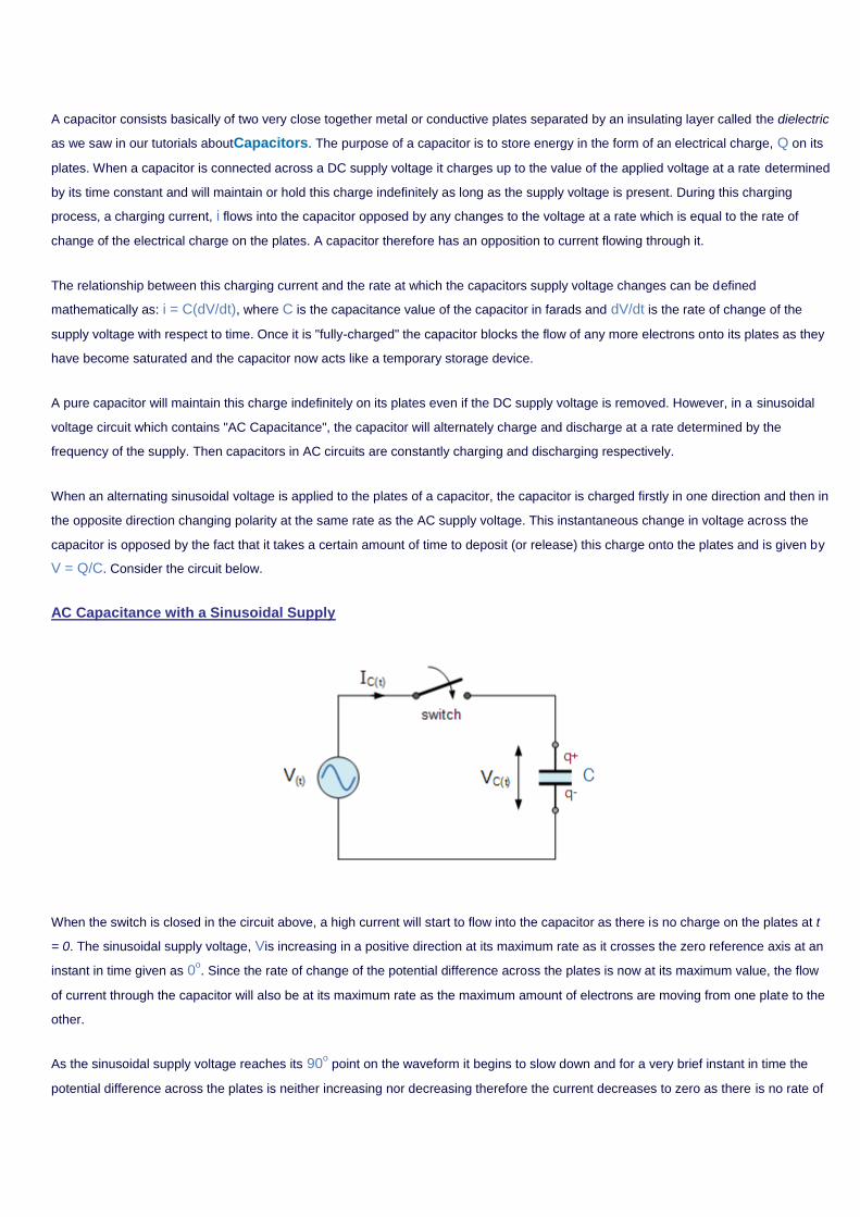
A capacitor consists basically of two very close together metal or conductive plates separated by an insulating layer called the dielectric

as we saw in our tutorials aboutCapacitors. The purpose of a capacitor is to store energy in the form of an electrical charge, Q on its

plates. When a capacitor is connected across a DC supply voltage it charges up to the value of the applied voltage at a rate determined

by its time constant and will maintain or hold this charge indefinitely as long as the supply voltage is present. During this charging

process, a charging current, i flows into the capacitor opposed by any changes to the voltage at a rate which is equal to the rate of

change of the electrical charge on the plates. A capacitor therefore has an opposition to current flowing through it.

The relationship between this charging current and the rate at which the capacitors supply voltage changes can be defined

mathematically as: i = C(dV/dt), where C is the capacitance value of the capacitor in farads and dV/dt is the rate of change of the

supply voltage with respect to time. Once it is "fully-charged" the capacitor blocks the flow of any more electrons onto its plates as they

have become saturated and the capacitor now acts like a temporary storage device.

A pure capacitor will maintain this charge indefinitely on its plates even if the DC supply voltage is removed. However, in a sinusoidal

voltage circuit which contains "AC Capacitance", the capacitor will alternately charge and discharge at a rate determined by the

frequency of the supply. Then capacitors in AC circuits are constantly charging and discharging respectively.

When an alternating sinusoidal voltage is applied to the plates of a capacitor, the capacitor is charged firstly in one direction and then in

the opposite direction changing polarity at the same rate as the AC supply voltage. This instantaneous change in voltage across the

capacitor is opposed by the fact that it takes a certain amount of time to deposit (or release) this charge onto the plates and is given by

V = Q/C. Consider the circuit below.

AC Capacitance with a Sinusoidal Supply

When the switch is closed in the circuit above, a high current will start to flow into the capacitor as there is no charge on the plates at t

= 0. The sinusoidal supply voltage, Vis increasing in a positive direction at its maximum rate as it crosses the zero reference axis at an

instant in time given as 0o. Since the rate of change of the potential difference across the plates is now at its maximum value, the flow

of current through the capacitor will also be at its maximum rate as the maximum amount of electrons are moving from one plate to the

other.

As the sinusoidal supply voltage reaches its 90o point on the waveform it begins to slow down and for a very brief instant in time the

potential difference across the plates is neither increasing nor decreasing therefore the current decreases to zero as there is no rate of

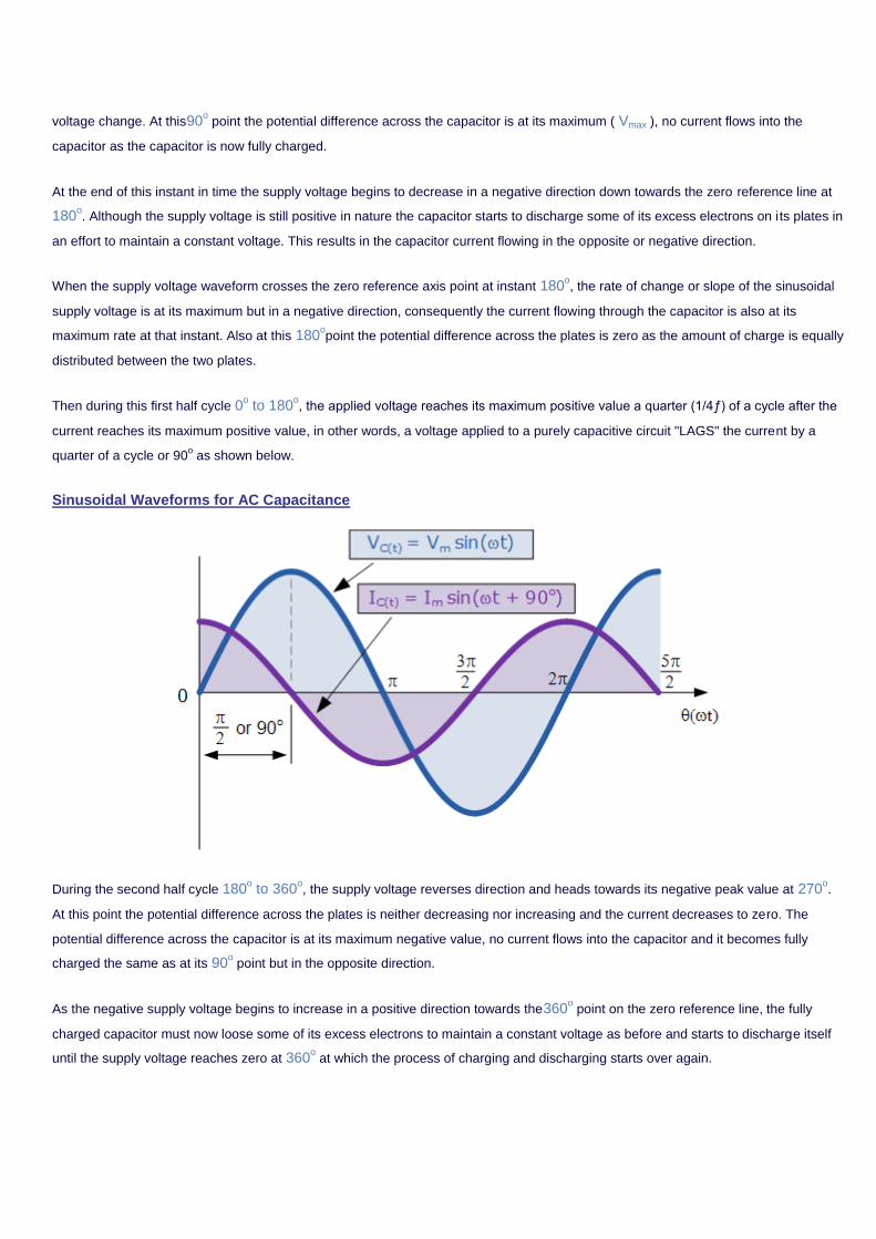
voltage change. At this90o point the potential difference across the capacitor is at its maximum ( Vmax ), no current flows into the

capacitor as the capacitor is now fully charged.

At the end of this instant in time the supply voltage begins to decrease in a negative direction down towards the zero reference line at

180o. Although the supply voltage is still positive in nature the capacitor starts to discharge some of its excess electrons on its plates in

an effort to maintain a constant voltage. This results in the capacitor current flowing in the opposite or negative direction.

When the supply voltage waveform crosses the zero reference axis point at instant 180o, the rate of change or slope of the sinusoidal

supply voltage is at its maximum but in a negative direction, consequently the current flowing through the capacitor is also at its

maximum rate at that instant. Also at this 180opoint the potential difference across the plates is zero as the amount of charge is equally

distributed between the two plates.

Then during this first half cycle 0o to 180

o, the applied voltage reaches its maximum positive value a quarter (1/4ƒ) of a cycle after the

current reaches its maximum positive value, in other words, a voltage applied to a purely capacitive circuit "LAGS" the current by a

quarter of a cycle or 90o as shown below.

Sinusoidal Waveforms for AC Capacitance

During the second half cycle 180o to 360

o, the supply voltage reverses direction and heads towards its negative peak value at 270

o.

At this point the potential difference across the plates is neither decreasing nor increasing and the current decreases to zero. The

potential difference across the capacitor is at its maximum negative value, no current flows into the capacitor and it becomes fully

charged the same as at its 90o point but in the opposite direction.

As the negative supply voltage begins to increase in a positive direction towards the360o point on the zero reference line, the fully

charged capacitor must now loose some of its excess electrons to maintain a constant voltage as before and starts to discharge itself

until the supply voltage reaches zero at 360o at which the process of charging and discharging starts over again.

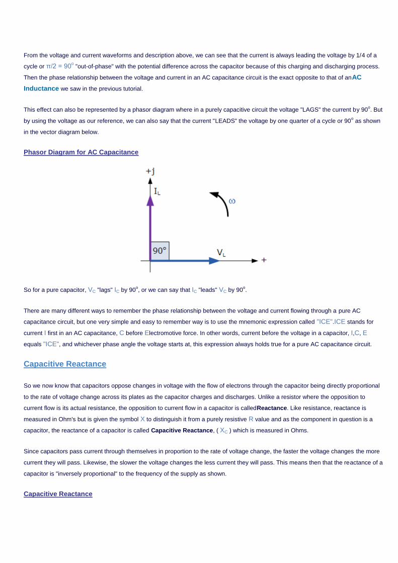
From the voltage and current waveforms and description above, we can see that the current is always leading the voltage by 1/4 of a

cycle or π/2 = 90o "out-of-phase" with the potential difference across the capacitor because of this charging and discharging process.

Then the phase relationship between the voltage and current in an AC capacitance circuit is the exact opposite to that of anAC

Inductance we saw in the previous tutorial.

This effect can also be represented by a phasor diagram where in a purely capacitive circuit the voltage "LAGS" the current by 90o. But

by using the voltage as our reference, we can also say that the current "LEADS" the voltage by one quarter of a cycle or 90o as shown

in the vector diagram below.

Phasor Diagram for AC Capacitance

So for a pure capacitor, VC "lags" IC by 90o, or we can say that IC "leads" VC by 90

o.

There are many different ways to remember the phase relationship between the voltage and current flowing through a pure AC

capacitance circuit, but one very simple and easy to remember way is to use the mnemonic expression called "ICE".ICE stands for

current I first in an AC capacitance, C before Electromotive force. In other words, current before the voltage in a capacitor, I,C, E

equals "ICE", and whichever phase angle the voltage starts at, this expression always holds true for a pure AC capacitance circuit.

Capacitive Reactance

So we now know that capacitors oppose changes in voltage with the flow of electrons through the capacitor being directly proportional

to the rate of voltage change across its plates as the capacitor charges and discharges. Unlike a resistor where the opposition to

current flow is its actual resistance, the opposition to current flow in a capacitor is calledReactance. Like resistance, reactance is

measured in Ohm's but is given the symbol X to distinguish it from a purely resistive R value and as the component in question is a

capacitor, the reactance of a capacitor is called Capacitive Reactance, ( XC ) which is measured in Ohms.

Since capacitors pass current through themselves in proportion to the rate of voltage change, the faster the voltage changes the more

current they will pass. Likewise, the slower the voltage changes the less current they will pass. This means then that the reactance of a

capacitor is "inversely proportional" to the frequency of the supply as shown.

Capacitive Reactance

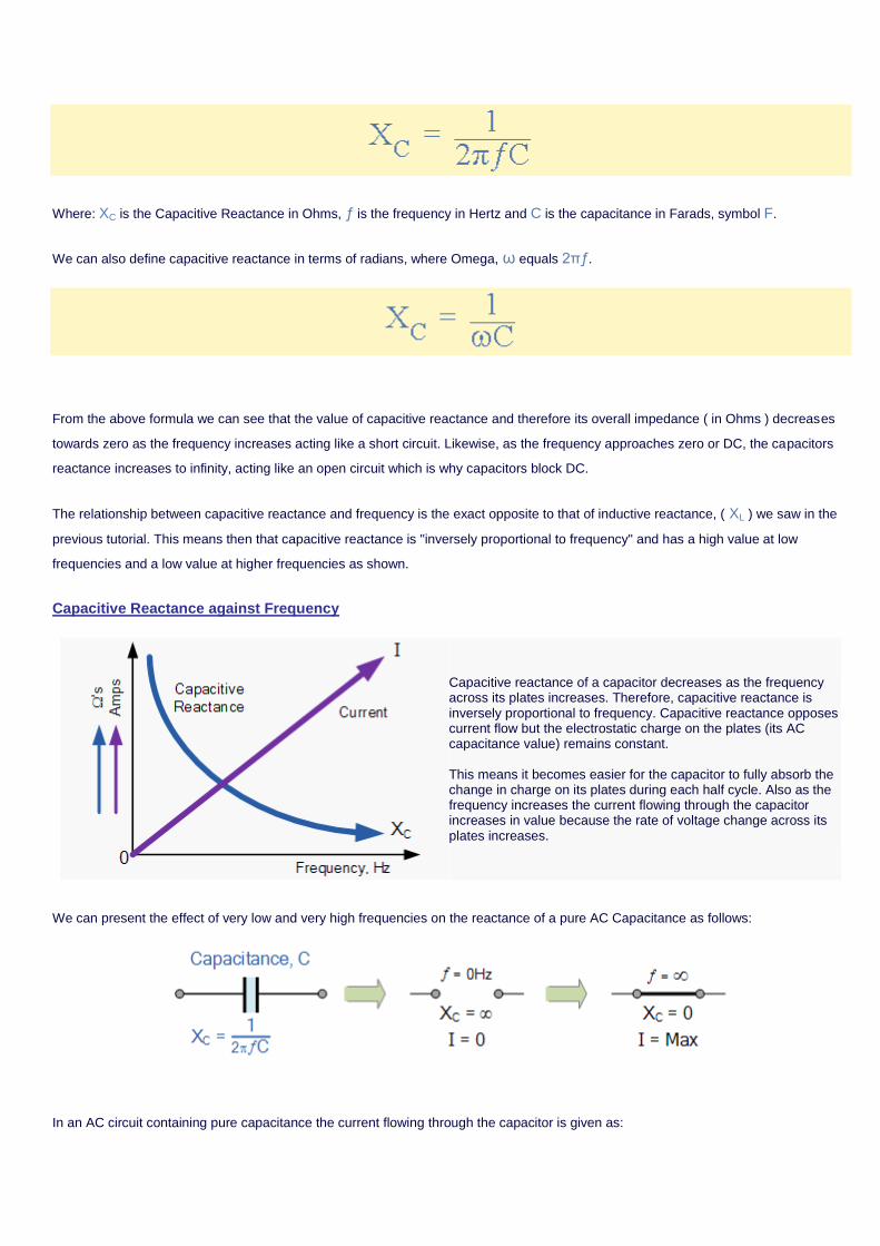
Where: XC is the Capacitive Reactance in Ohms, ƒ is the frequency in Hertz and C is the capacitance in Farads, symbol F.

We can also define capacitive reactance in terms of radians, where Omega, ω equals 2πƒ.

From the above formula we can see that the value of capacitive reactance and therefore its overall impedance ( in Ohms ) decreases

towards zero as the frequency increases acting like a short circuit. Likewise, as the frequency approaches zero or DC, the capacitors

reactance increases to infinity, acting like an open circuit which is why capacitors block DC.

The relationship between capacitive reactance and frequency is the exact opposite to that of inductive reactance, ( XL ) we saw in the

previous tutorial. This means then that capacitive reactance is "inversely proportional to frequency" and has a high value at low

frequencies and a low value at higher frequencies as shown.

Capacitive Reactance against Frequency

Capacitive reactance of a capacitor decreases as the frequency across its plates increases. Therefore, capacitive reactance is inversely proportional to frequency. Capacitive reactance opposes current flow but the electrostatic charge on the plates (its AC capacitance value) remains constant. This means it becomes easier for the capacitor to fully absorb the change in charge on its plates during each half cycle. Also as the frequency increases the current flowing through the capacitor increases in value because the rate of voltage change across its plates increases.

We can present the effect of very low and very high frequencies on the reactance of a pure AC Capacitance as follows:

In an AC circuit containing pure capacitance the current flowing through the capacitor is given as:

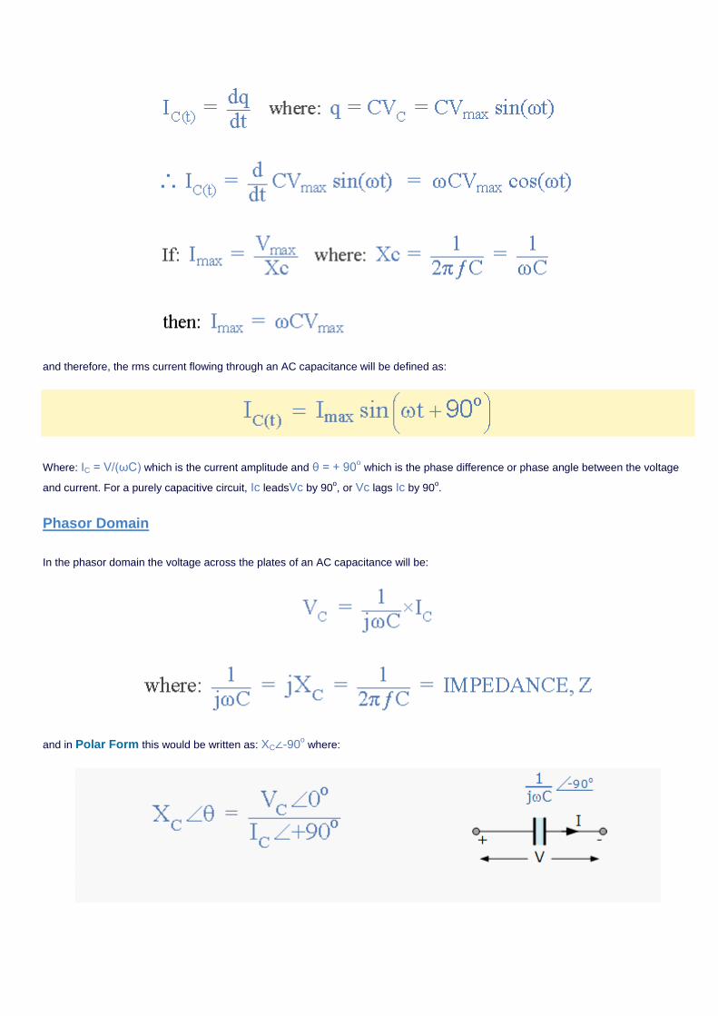
and therefore, the rms current flowing through an AC capacitance will be defined as:

Where: IC = V/(ωC) which is the current amplitude and θ = + 90o which is the phase difference or phase angle between the voltage

and current. For a purely capacitive circuit, Ic leadsVc by 90o, or Vc lags Ic by 90

o.

Phasor Domain

In the phasor domain the voltage across the plates of an AC capacitance will be:

and in Polar Form this would be written as: XC∠-90o where:

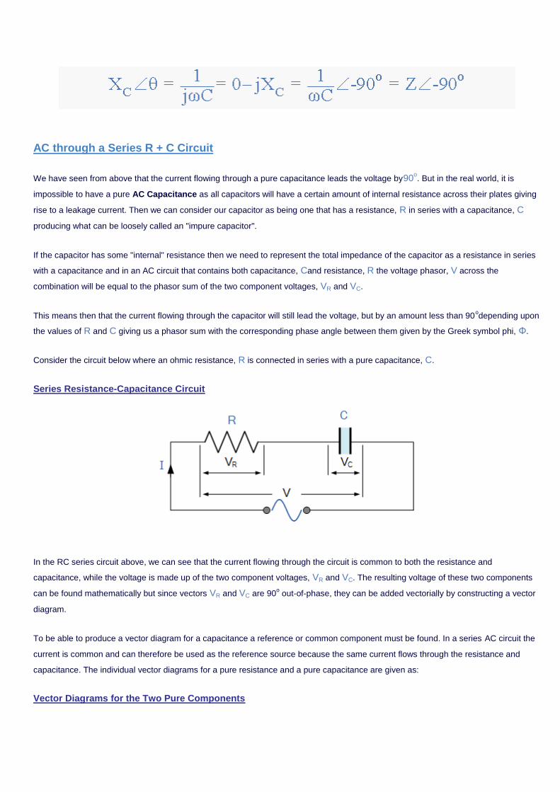
AC through a Series R + C Circuit

We have seen from above that the current flowing through a pure capacitance leads the voltage by90o. But in the real world, it is

impossible to have a pure AC Capacitance as all capacitors will have a certain amount of internal resistance across their plates giving

rise to a leakage current. Then we can consider our capacitor as being one that has a resistance, R in series with a capacitance, C

producing what can be loosely called an "impure capacitor".

If the capacitor has some "internal" resistance then we need to represent the total impedance of the capacitor as a resistance in series

with a capacitance and in an AC circuit that contains both capacitance, Cand resistance, R the voltage phasor, V across the

combination will be equal to the phasor sum of the two component voltages, VR and VC.

This means then that the current flowing through the capacitor will still lead the voltage, but by an amount less than 90odepending upon

the values of R and C giving us a phasor sum with the corresponding phase angle between them given by the Greek symbol phi, Φ.

Consider the circuit below where an ohmic resistance, R is connected in series with a pure capacitance, C.

Series Resistance-Capacitance Circuit

In the RC series circuit above, we can see that the current flowing through the circuit is common to both the resistance and

capacitance, while the voltage is made up of the two component voltages, VR and VC. The resulting voltage of these two components

can be found mathematically but since vectors VR and VC are 90o out-of-phase, they can be added vectorially by constructing a vector

diagram.

To be able to produce a vector diagram for a capacitance a reference or common component must be found. In a series AC circuit the

current is common and can therefore be used as the reference source because the same current flows through the resistance and

capacitance. The individual vector diagrams for a pure resistance and a pure capacitance are given as:

Vector Diagrams for the Two Pure Components

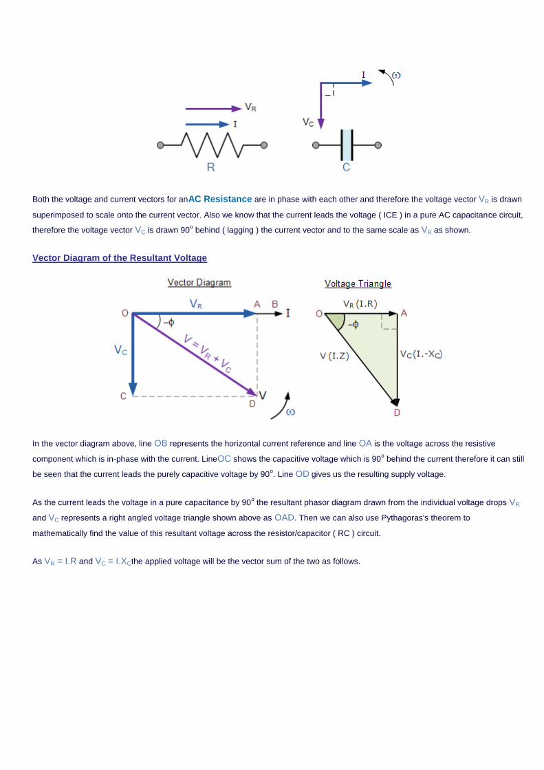
Both the voltage and current vectors for anAC Resistance are in phase with each other and therefore the voltage vector VR is drawn

superimposed to scale onto the current vector. Also we know that the current leads the voltage ( ICE ) in a pure AC capacitance circuit,

therefore the voltage vector VC is drawn 90o behind ( lagging ) the current vector and to the same scale as VR as shown.

Vector Diagram of the Resultant Voltage

In the vector diagram above, line OB represents the horizontal current reference and line OA is the voltage across the resistive

component which is in-phase with the current. LineOC shows the capacitive voltage which is 90o behind the current therefore it can still

be seen that the current leads the purely capacitive voltage by 90o. Line OD gives us the resulting supply voltage.

As the current leads the voltage in a pure capacitance by 90o the resultant phasor diagram drawn from the individual voltage drops VR

and VC represents a right angled voltage triangle shown above as OAD. Then we can also use Pythagoras's theorem to

mathematically find the value of this resultant voltage across the resistor/capacitor ( RC ) circuit.

As VR = I.R and VC = I.XCthe applied voltage will be the vector sum of the two as follows.

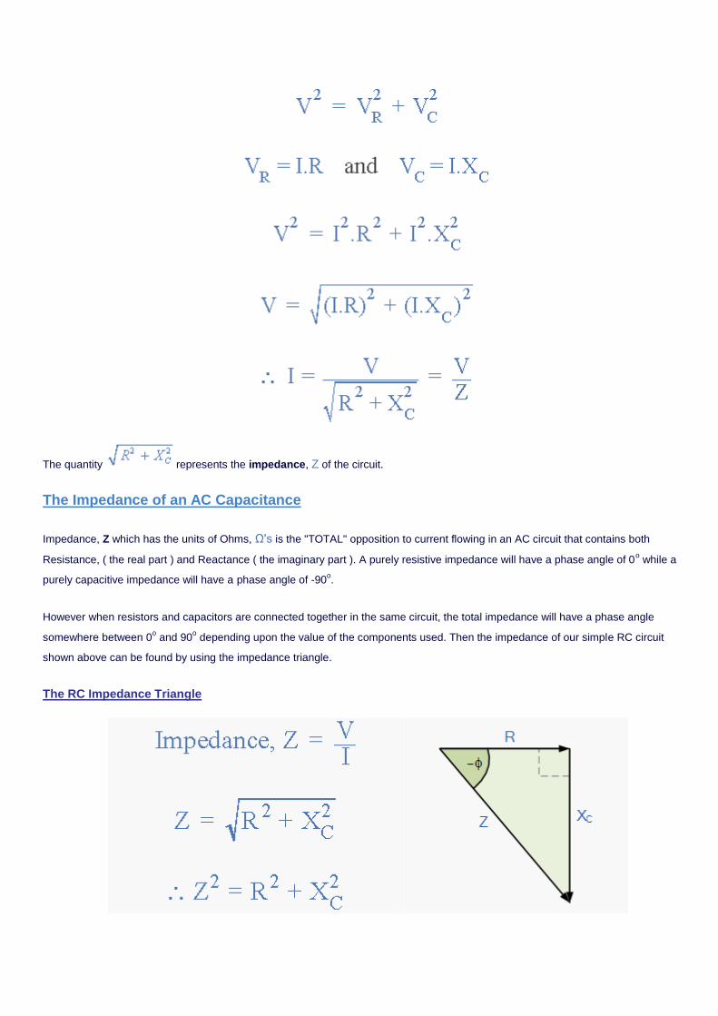
The quantity represents the impedance, Z of the circuit.

The Impedance of an AC Capacitance

Impedance, Z which has the units of Ohms, Ω's is the "TOTAL" opposition to current flowing in an AC circuit that contains both

Resistance, ( the real part ) and Reactance ( the imaginary part ). A purely resistive impedance will have a phase angle of 0o while a

purely capacitive impedance will have a phase angle of -90o.

However when resistors and capacitors are connected together in the same circuit, the total impedance will have a phase angle

somewhere between 0o and 90

o depending upon the value of the components used. Then the impedance of our simple RC circuit

shown above can be found by using the impedance triangle.

The RC Impedance Triangle

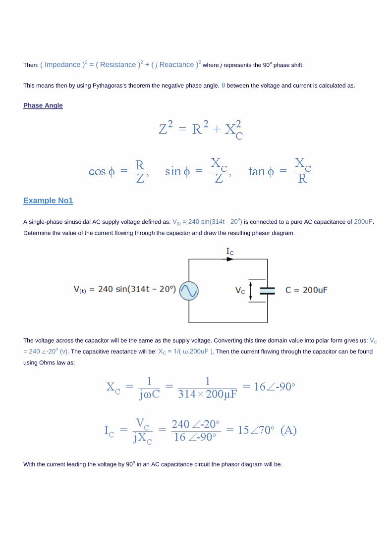
Then: ( Impedance )2 = ( Resistance )2 + ( j Reactance )2 where j represents the 90

o phase shift.

This means then by using Pythagoras's theorem the negative phase angle, θ between the voltage and current is calculated as.

Phase Angle

Example No1

A single-phase sinusoidal AC supply voltage defined as: V(t) = 240 sin(314t - 20o) is connected to a pure AC capacitance of 200uF.

Determine the value of the current flowing through the capacitor and draw the resulting phasor diagram.

The voltage across the capacitor will be the same as the supply voltage. Converting this time domain value into polar form gives us: VC

= 240 ∠-20o (v). The capacitive reactance will be: XC = 1/( ω.200uF ). Then the current flowing through the capacitor can be found

using Ohms law as:

With the current leading the voltage by 90o in an AC capacitance circuit the phasor diagram will be.

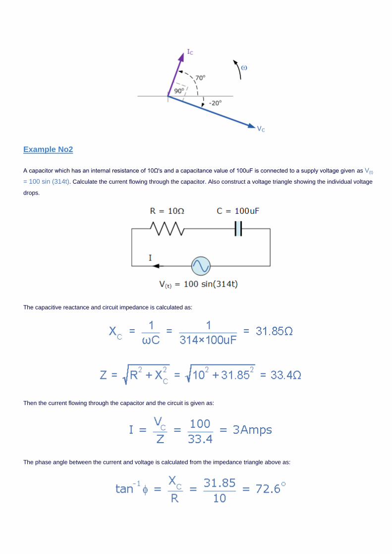
Example No2

A capacitor which has an internal resistance of 10Ω's and a capacitance value of 100uF is connected to a supply voltage given as V(t)

= 100 sin (314t). Calculate the current flowing through the capacitor. Also construct a voltage triangle showing the individual voltage

drops.

The capacitive reactance and circuit impedance is calculated as:

Then the current flowing through the capacitor and the circuit is given as:

The phase angle between the current and voltage is calculated from the impedance triangle above as:

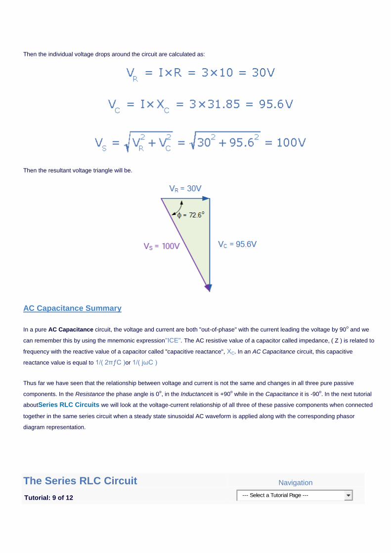
Then the individual voltage drops around the circuit are calculated as:

Then the resultant voltage triangle will be.

AC Capacitance Summary

In a pure AC Capacitance circuit, the voltage and current are both "out-of-phase" with the current leading the voltage by 90o and we

can remember this by using the mnemonic expression"ICE". The AC resistive value of a capacitor called impedance, ( Z ) is related to

frequency with the reactive value of a capacitor called "capacitive reactance", XC. In an AC Capacitance circuit, this capacitive

reactance value is equal to 1/( 2πƒC )or 1/( jωC )

Thus far we have seen that the relationship between voltage and current is not the same and changes in all three pure passive

components. In the Resistance the phase angle is 0o, in the Inductanceit is +90

o while in the Capacitance it is -90

o. In the next tutorial

aboutSeries RLC Circuits we will look at the voltage-current relationship of all three of these passive components when connected

together in the same series circuit when a steady state sinusoidal AC waveform is applied along with the corresponding phasor

diagram representation.

The Series RLC Circuit Navigation

Tutorial: 9 of 12 --- Select a Tutorial Page ---

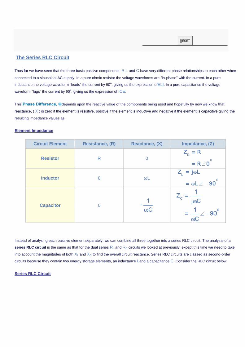
RESET

The Series RLC Circuit

Thus far we have seen that the three basic passive components, R,L and C have very different phase relationships to each other when

connected to a sinusoidal AC supply. In a pure ohmic resistor the voltage waveforms are "in-phase" with the current. In a pure

inductance the voltage waveform "leads" the current by 90o, giving us the expression ofELI. In a pure capacitance the voltage

waveform "lags" the current by 90o, giving us the expression of ICE.

This Phase Difference, Φdepends upon the reactive value of the components being used and hopefully by now we know that

reactance, ( X ) is zero if the element is resistive, positive if the element is inductive and negative if the element is capacitive giving the

resulting impedance values as:

Element Impedance

Circuit Element Resistance, (R) Reactance, (X) Impedance, (Z)

Resistor R 0

Inductor 0 ωL

Capacitor 0

Instead of analysing each passive element separately, we can combine all three together into a series RLC circuit. The analysis of a

series RLC circuit is the same as that for the dual series RL and RC circuits we looked at previously, except this time we need to take

into account the magnitudes of both XL and XC to find the overall circuit reactance. Series RLC circuits are classed as second-order

circuits because they contain two energy storage elements, an inductance Land a capacitance C. Consider the RLC circuit below.

Series RLC Circuit

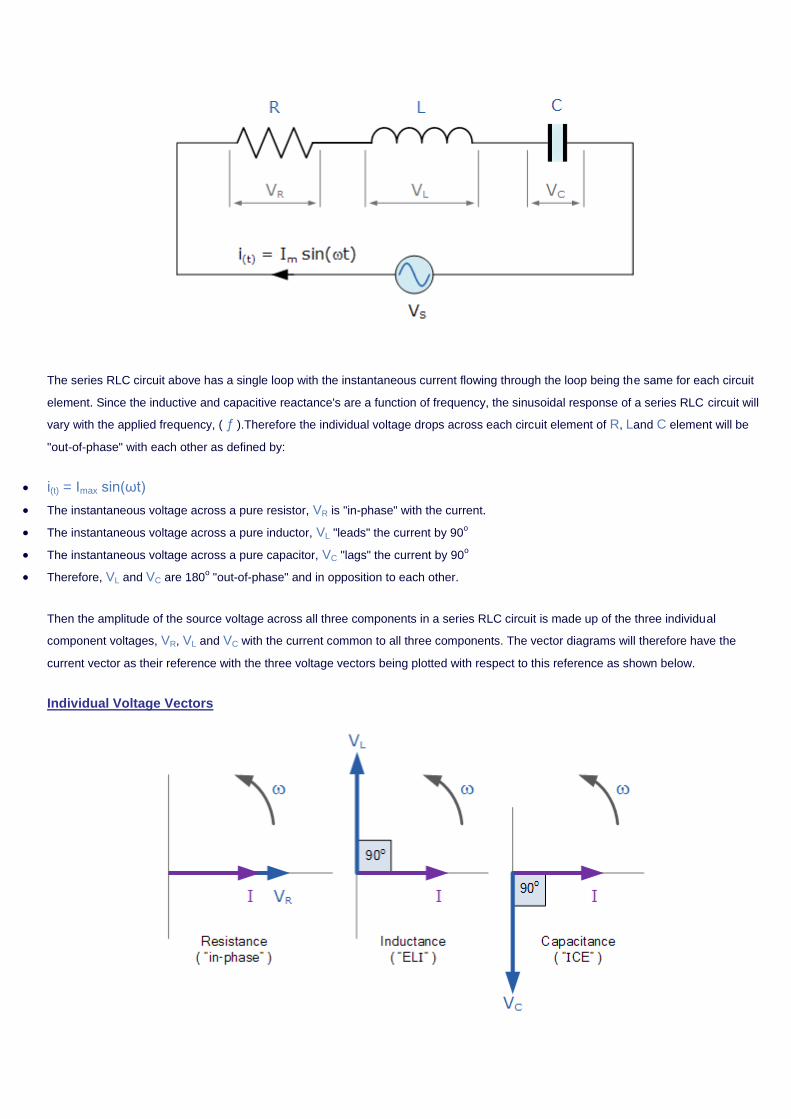
The series RLC circuit above has a single loop with the instantaneous current flowing through the loop being the same for each circuit

element. Since the inductive and capacitive reactance's are a function of frequency, the sinusoidal response of a series RLC circuit will

vary with the applied frequency, ( ƒ ).Therefore the individual voltage drops across each circuit element of R, Land C element will be

"out-of-phase" with each other as defined by:

i(t) = Imax sin(ωt)

The instantaneous voltage across a pure resistor, VR is "in-phase" with the current.

The instantaneous voltage across a pure inductor, VL "leads" the current by 90o

The instantaneous voltage across a pure capacitor, VC "lags" the current by 90o

Therefore, VL and VC are 180o "out-of-phase" and in opposition to each other.

Then the amplitude of the source voltage across all three components in a series RLC circuit is made up of the three individual

component voltages, VR, VL and VC with the current common to all three components. The vector diagrams will therefore have the

current vector as their reference with the three voltage vectors being plotted with respect to this reference as shown below.

Individual Voltage Vectors

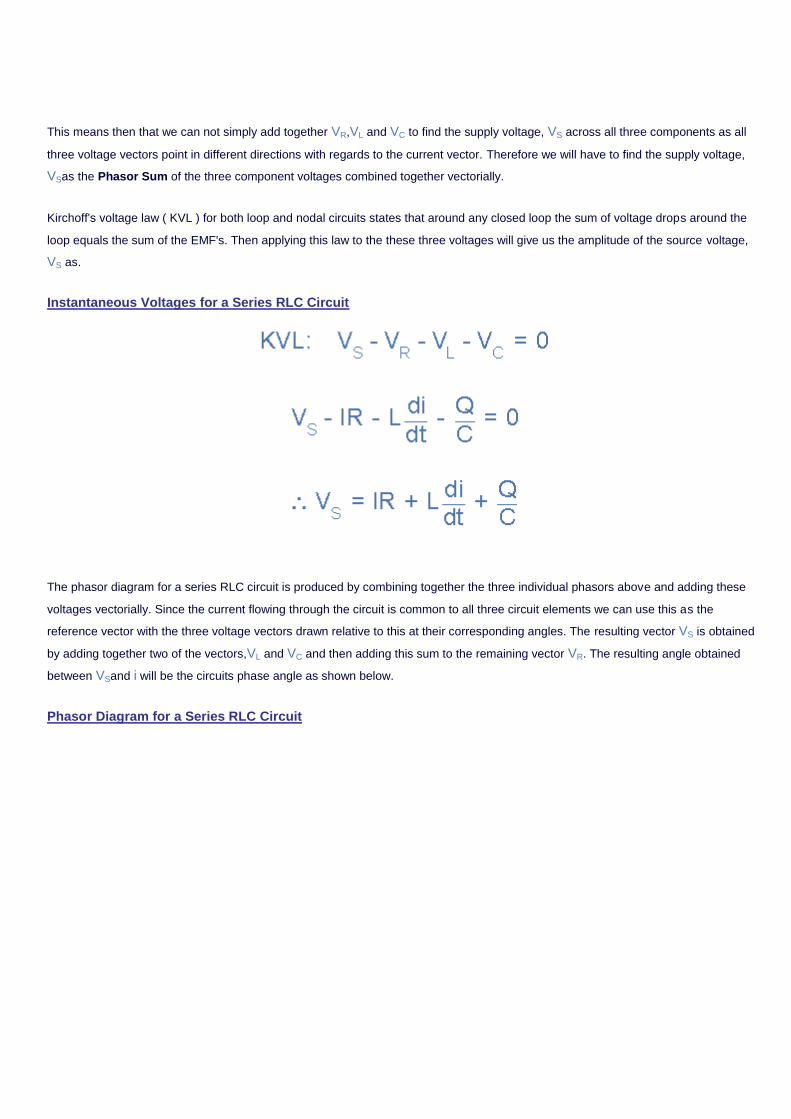
This means then that we can not simply add together VR,VL and VC to find the supply voltage, VS across all three components as all

three voltage vectors point in different directions with regards to the current vector. Therefore we will have to find the supply voltage,

VSas the Phasor Sum of the three component voltages combined together vectorially.

Kirchoff's voltage law ( KVL ) for both loop and nodal circuits states that around any closed loop the sum of voltage drops around the

loop equals the sum of the EMF's. Then applying this law to the these three voltages will give us the amplitude of the source voltage,

VS as.

Instantaneous Voltages for a Series RLC Circuit

The phasor diagram for a series RLC circuit is produced by combining together the three individual phasors above and adding these

voltages vectorially. Since the current flowing through the circuit is common to all three circuit elements we can use this as the

reference vector with the three voltage vectors drawn relative to this at their corresponding angles. The resulting vector VS is obtained

by adding together two of the vectors,VL and VC and then adding this sum to the remaining vector VR. The resulting angle obtained

between VSand i will be the circuits phase angle as shown below.

Phasor Diagram for a Series RLC Circuit

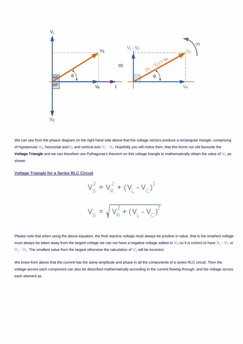
We can see from the phasor diagram on the right hand side above that the voltage vectors produce a rectangular triangle, comprising

of hypotenuse VS, horizontal axisVR and vertical axis VL - VC Hopefully you will notice then, that this forms our old favourite the

Voltage Triangle and we can therefore use Pythagoras's theorem on this voltage triangle to mathematically obtain the value of VS as

shown.

Voltage Triangle for a Series RLC Circuit

Please note that when using the above equation, the final reactive voltage must always be positive in value, that is the smallest voltage

must always be taken away from the largest voltage we can not have a negative voltage added to VR so it is correct to have VL - VC or

VC - VL. The smallest value from the largest otherwise the calculation of VS will be incorrect.

We know from above that the current has the same amplitude and phase in all the components of a series RLC circuit. Then the

voltage across each component can also be described mathematically according to the current flowing through, and the voltage across

each element as.

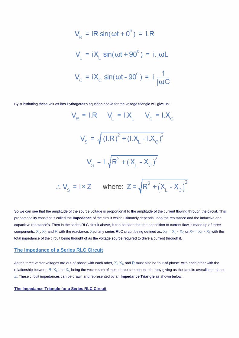
By substituting these values into Pythagoras's equation above for the voltage triangle will give us:

So we can see that the amplitude of the source voltage is proportional to the amplitude of the current flowing through the circuit. This

proportionality constant is called the Impedance of the circuit which ultimately depends upon the resistance and the inductive and

capacitive reactance's. Then in the series RLC circuit above, it can be seen that the opposition to current flow is made up of three

components, XL, XC and R with the reactance, XTof any series RLC circuit being defined as: XT = XL - XC or XT = XC - XL with the

total impedance of the circuit being thought of as the voltage source required to drive a current through it.

The Impedance of a Series RLC Circuit

As the three vector voltages are out-of-phase with each other, XL,XC and R must also be "out-of-phase" with each other with the

relationship between R, XL and XC being the vector sum of these three components thereby giving us the circuits overall impedance,

Z. These circuit impedances can be drawn and represented by an Impedance Triangle as shown below.

The Impedance Triangle for a Series RLC Circuit

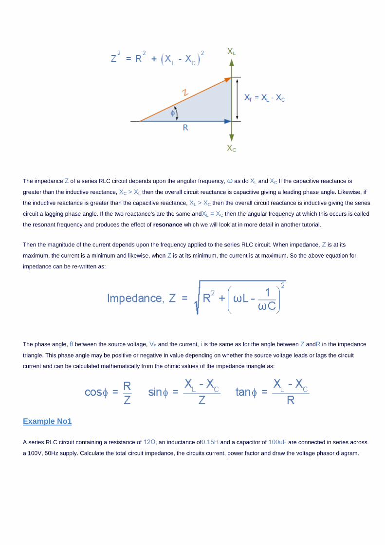
The impedance Z of a series RLC circuit depends upon the angular frequency, ω as do XL and XC If the capacitive reactance is

greater than the inductive reactance, XC > XL then the overall circuit reactance is capacitive giving a leading phase angle. Likewise, if

the inductive reactance is greater than the capacitive reactance, XL > XC then the overall circuit reactance is inductive giving the series

circuit a lagging phase angle. If the two reactance's are the same andXL = XC then the angular frequency at which this occurs is called

the resonant frequency and produces the effect of resonance which we will look at in more detail in another tutorial.

Then the magnitude of the current depends upon the frequency applied to the series RLC circuit. When impedance, Z is at its

maximum, the current is a minimum and likewise, when Z is at its minimum, the current is at maximum. So the above equation for

impedance can be re-written as:

The phase angle, θ between the source voltage, VS and the current, i is the same as for the angle between Z andR in the impedance

triangle. This phase angle may be positive or negative in value depending on whether the source voltage leads or lags the circuit

current and can be calculated mathematically from the ohmic values of the impedance triangle as:

Example No1

A series RLC circuit containing a resistance of 12Ω, an inductance of0.15H and a capacitor of 100uF are connected in series across

a 100V, 50Hz supply. Calculate the total circuit impedance, the circuits current, power factor and draw the voltage phasor diagram.

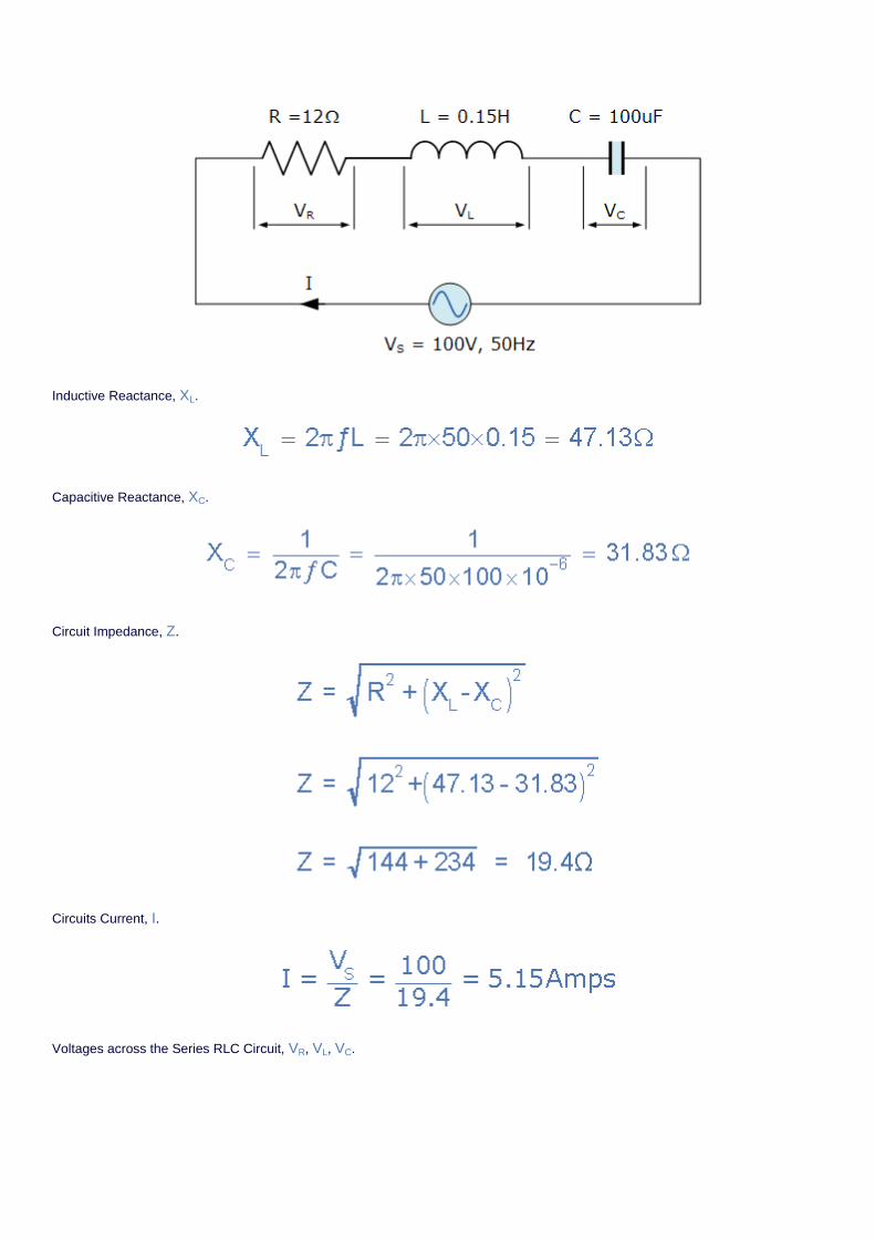
Inductive Reactance, XL.

Capacitive Reactance, XC.

Circuit Impedance, Z.

Circuits Current, I.

Voltages across the Series RLC Circuit, VR, VL, VC.

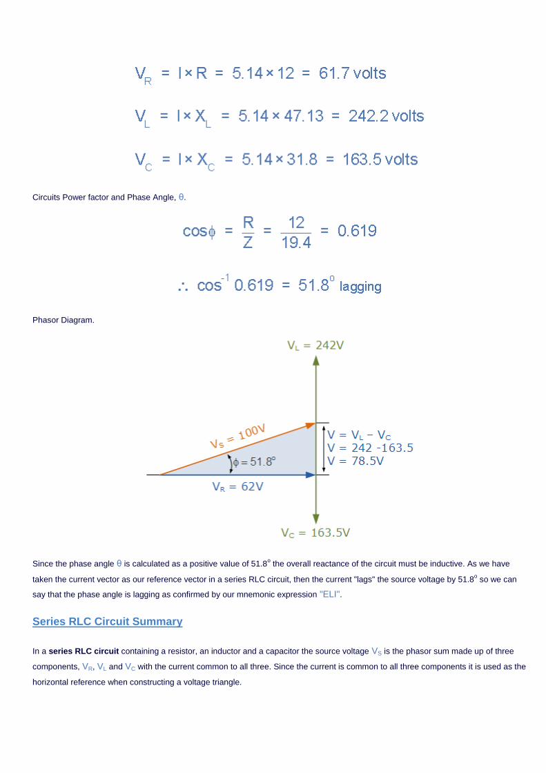
Circuits Power factor and Phase Angle, θ.

Phasor Diagram.

Since the phase angle θ is calculated as a positive value of 51.8o the overall reactance of the circuit must be inductive. As we have

taken the current vector as our reference vector in a series RLC circuit, then the current "lags" the source voltage by 51.8o so we can

say that the phase angle is lagging as confirmed by our mnemonic expression "ELI".

Series RLC Circuit Summary

In a series RLC circuit containing a resistor, an inductor and a capacitor the source voltage VS is the phasor sum made up of three

components, VR, VL and VC with the current common to all three. Since the current is common to all three components it is used as the

horizontal reference when constructing a voltage triangle.

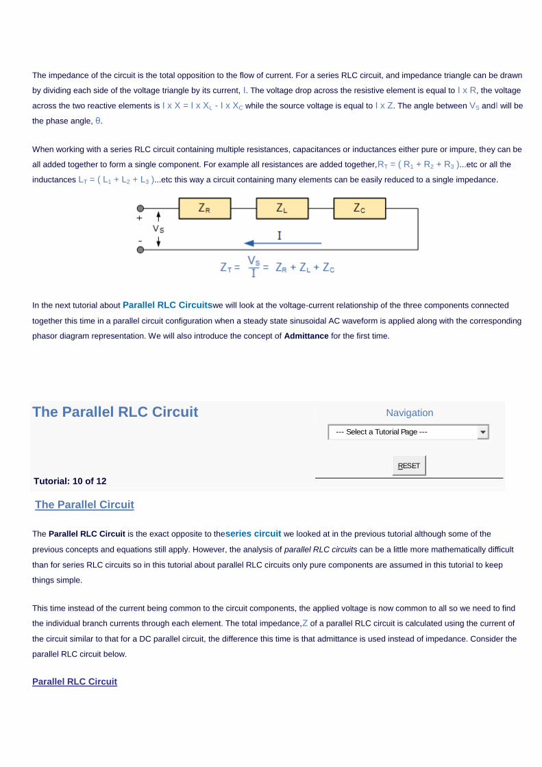
The impedance of the circuit is the total opposition to the flow of current. For a series RLC circuit, and impedance triangle can be drawn

by dividing each side of the voltage triangle by its current, I. The voltage drop across the resistive element is equal to I x R, the voltage

across the two reactive elements is I x X = I x XL - I x XC while the source voltage is equal to I x Z. The angle between VS andI will be

the phase angle, θ.

When working with a series RLC circuit containing multiple resistances, capacitances or inductances either pure or impure, they can be

all added together to form a single component. For example all resistances are added together,RT = ( R1 + R2 + R3 )...etc or all the

inductances LT = ( L1 + L2 + L3 )...etc this way a circuit containing many elements can be easily reduced to a single impedance.

In the next tutorial about Parallel RLC Circuitswe will look at the voltage-current relationship of the three components connected

together this time in a parallel circuit configuration when a steady state sinusoidal AC waveform is applied along with the corresponding

phasor diagram representation. We will also introduce the concept of Admittance for the first time.

The Parallel RLC Circuit Navigation

Tutorial: 10 of 12

--- Select a Tutorial Page ---

RESET

The Parallel Circuit

The Parallel RLC Circuit is the exact opposite to theseries circuit we looked at in the previous tutorial although some of the

previous concepts and equations still apply. However, the analysis of parallel RLC circuits can be a little more mathematically difficult

than for series RLC circuits so in this tutorial about parallel RLC circuits only pure components are assumed in this tutorial to keep

things simple.

This time instead of the current being common to the circuit components, the applied voltage is now common to all so we need to find

the individual branch currents through each element. The total impedance,Z of a parallel RLC circuit is calculated using the current of

the circuit similar to that for a DC parallel circuit, the difference this time is that admittance is used instead of impedance. Consider the

parallel RLC circuit below.

Parallel RLC Circuit

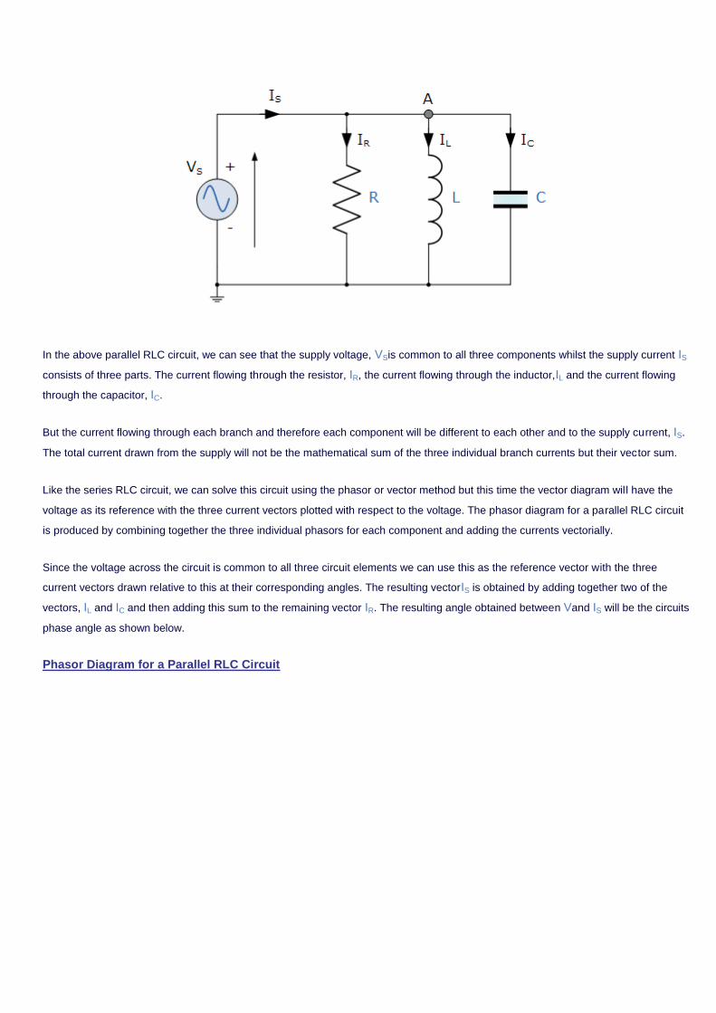
In the above parallel RLC circuit, we can see that the supply voltage, VSis common to all three components whilst the supply current IS

consists of three parts. The current flowing through the resistor, IR, the current flowing through the inductor,IL and the current flowing

through the capacitor, IC.

But the current flowing through each branch and therefore each component will be different to each other and to the supply current, IS.

The total current drawn from the supply will not be the mathematical sum of the three individual branch currents but their vector sum.

Like the series RLC circuit, we can solve this circuit using the phasor or vector method but this time the vector diagram will have the

voltage as its reference with the three current vectors plotted with respect to the voltage. The phasor diagram for a parallel RLC circuit

is produced by combining together the three individual phasors for each component and adding the currents vectorially.

Since the voltage across the circuit is common to all three circuit elements we can use this as the reference vector with the three

current vectors drawn relative to this at their corresponding angles. The resulting vectorIS is obtained by adding together two of the

vectors, IL and IC and then adding this sum to the remaining vector IR. The resulting angle obtained between Vand IS will be the circuits

phase angle as shown below.

Phasor Diagram for a Parallel RLC Circuit

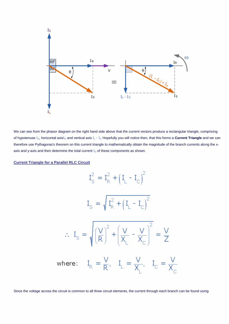
We can see from the phasor diagram on the right hand side above that the current vectors produce a rectangular triangle, comprising

of hypotenuse IS, horizontal axisIR and vertical axis IL - IC Hopefully you will notice then, that this forms a Current Triangle and we can

therefore use Pythagoras's theorem on this current triangle to mathematically obtain the magnitude of the branch currents along the x-

axis and y-axis and then determine the total current IS of these components as shown.

Current Triangle for a Parallel RLC Circuit

Since the voltage across the circuit is common to all three circuit elements, the current through each branch can be found using

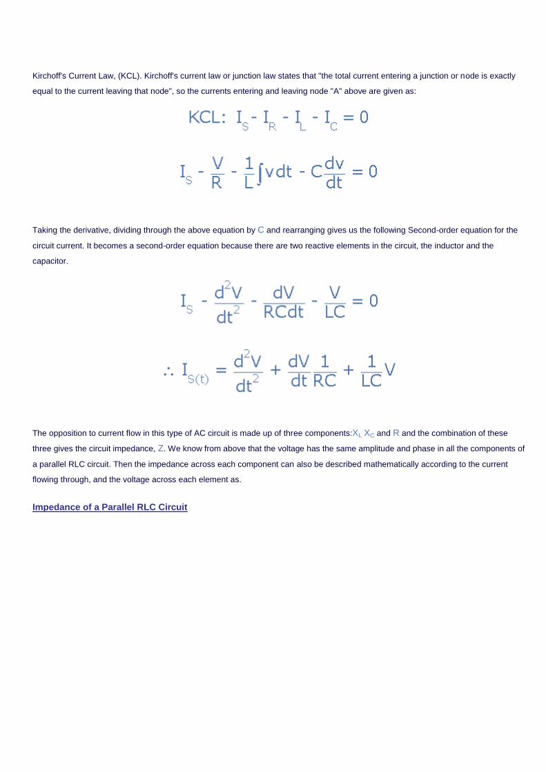
Kirchoff's Current Law, (KCL). Kirchoff's current law or junction law states that "the total current entering a junction or node is exactly

equal to the current leaving that node", so the currents entering and leaving node "A" above are given as:

Taking the derivative, dividing through the above equation by C and rearranging gives us the following Second-order equation for the

circuit current. It becomes a second-order equation because there are two reactive elements in the circuit, the inductor and the

capacitor.

The opposition to current flow in this type of AC circuit is made up of three components:XL XC and R and the combination of these

three gives the circuit impedance, Z. We know from above that the voltage has the same amplitude and phase in all the components of

a parallel RLC circuit. Then the impedance across each component can also be described mathematically according to the current

flowing through, and the voltage across each element as.

Impedance of a Parallel RLC Circuit

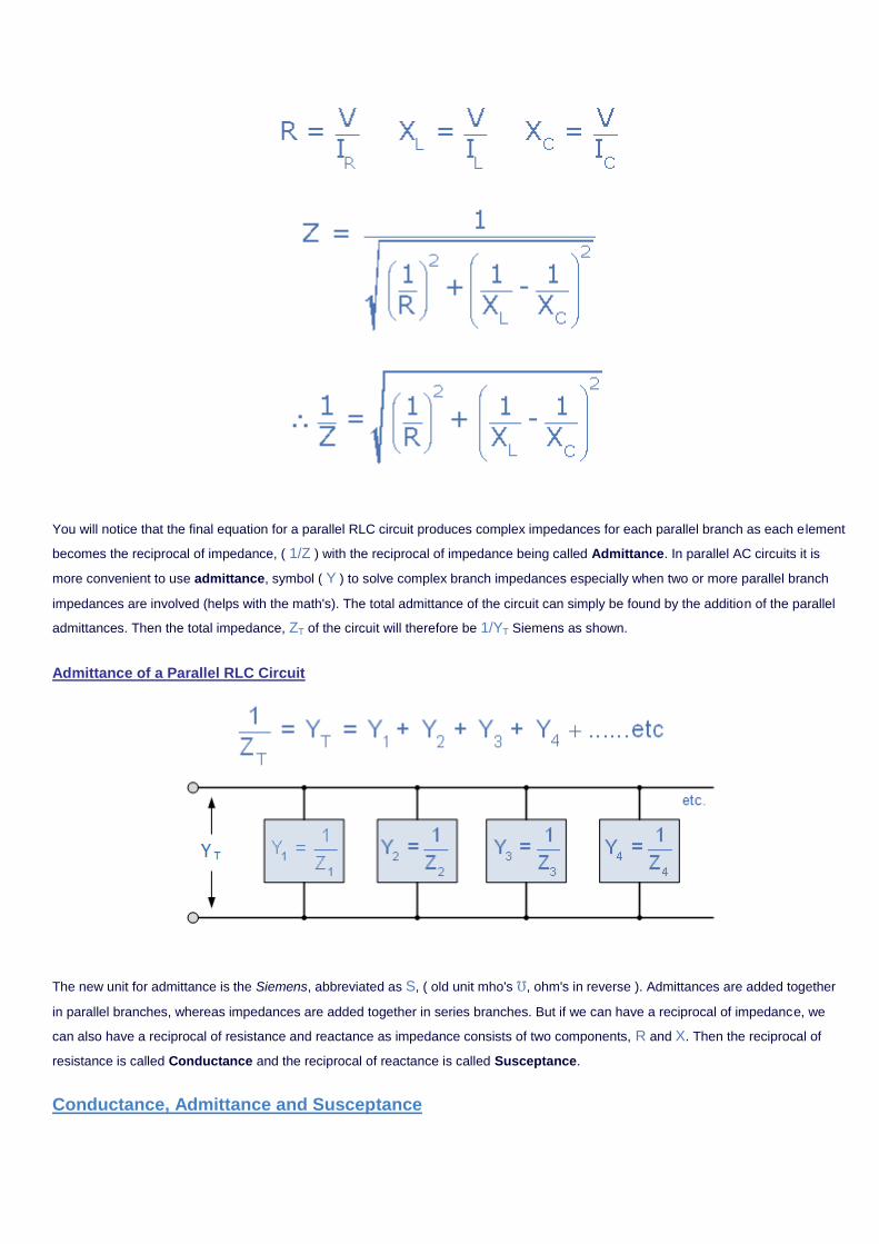
You will notice that the final equation for a parallel RLC circuit produces complex impedances for each parallel branch as each element

becomes the reciprocal of impedance, ( 1/Z ) with the reciprocal of impedance being called Admittance. In parallel AC circuits it is

more convenient to use admittance, symbol ( Y ) to solve complex branch impedances especially when two or more parallel branch

impedances are involved (helps with the math's). The total admittance of the circuit can simply be found by the addition of the parallel

admittances. Then the total impedance, ZT of the circuit will therefore be 1/YT Siemens as shown.

Admittance of a Parallel RLC Circuit

The new unit for admittance is the Siemens, abbreviated as S, ( old unit mho's ℧, ohm's in reverse ). Admittances are added together

in parallel branches, whereas impedances are added together in series branches. But if we can have a reciprocal of impedance, we

can also have a reciprocal of resistance and reactance as impedance consists of two components, R and X. Then the reciprocal of

resistance is called Conductance and the reciprocal of reactance is called Susceptance.

Conductance, Admittance and Susceptance

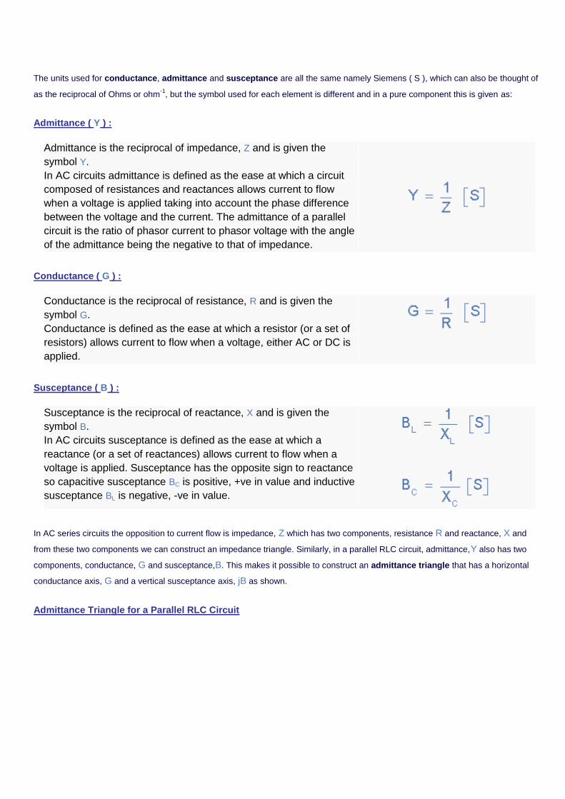
The units used for conductance, admittance and susceptance are all the same namely Siemens ( S ), which can also be thought of

as the reciprocal of Ohms or ohm-1

, but the symbol used for each element is different and in a pure component this is given as:

Admittance ( Y ) :

Admittance is the reciprocal of impedance, Z and is given the

symbol Y.

In AC circuits admittance is defined as the ease at which a circuit

composed of resistances and reactances allows current to flow

when a voltage is applied taking into account the phase difference

between the voltage and the current. The admittance of a parallel

circuit is the ratio of phasor current to phasor voltage with the angle

of the admittance being the negative to that of impedance.

Conductance ( G ) :

Conductance is the reciprocal of resistance, R and is given the

symbol G.

Conductance is defined as the ease at which a resistor (or a set of

resistors) allows current to flow when a voltage, either AC or DC is

applied.

Susceptance ( B ) :

Susceptance is the reciprocal of reactance, X and is given the

symbol B.

In AC circuits susceptance is defined as the ease at which a

reactance (or a set of reactances) allows current to flow when a

voltage is applied. Susceptance has the opposite sign to reactance

so capacitive susceptance BC is positive, +ve in value and inductive

susceptance BL is negative, -ve in value.

In AC series circuits the opposition to current flow is impedance, Z which has two components, resistance R and reactance, X and

from these two components we can construct an impedance triangle. Similarly, in a parallel RLC circuit, admittance,Y also has two

components, conductance, G and susceptance,B. This makes it possible to construct an admittance triangle that has a horizontal

conductance axis, G and a vertical susceptance axis, jB as shown.

Admittance Triangle for a Parallel RLC Circuit

Now that we have an admittance triangle, we can use Pythagoras to calculate the magnitudes of all three sides as well as the phase

angle as shown.

from Pythagoras,

Then we can define both the admittance of the circuit and the impedance with respect to admittance as:

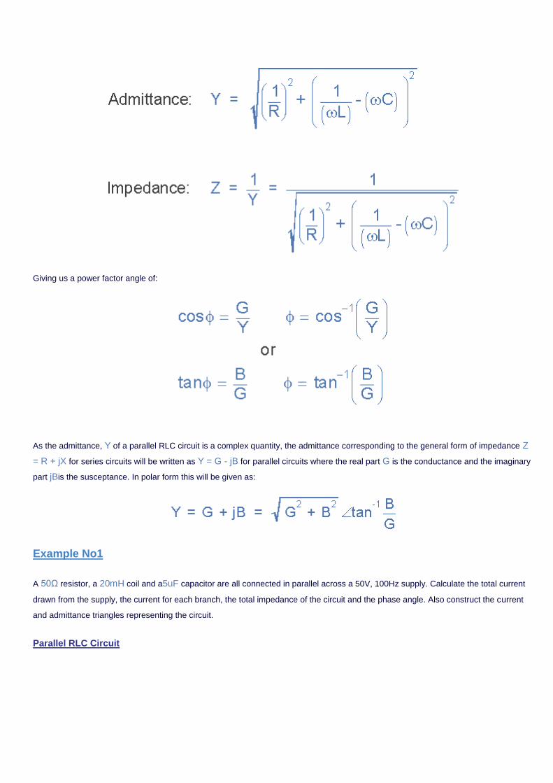
Giving us a power factor angle of:

As the admittance, Y of a parallel RLC circuit is a complex quantity, the admittance corresponding to the general form of impedance Z

= R + jX for series circuits will be written as Y = G - jB for parallel circuits where the real part G is the conductance and the imaginary

part jBis the susceptance. In polar form this will be given as:

Example No1

A 50Ω resistor, a 20mH coil and a5uF capacitor are all connected in parallel across a 50V, 100Hz supply. Calculate the total current

drawn from the supply, the current for each branch, the total impedance of the circuit and the phase angle. Also construct the current

and admittance triangles representing the circuit.

Parallel RLC Circuit

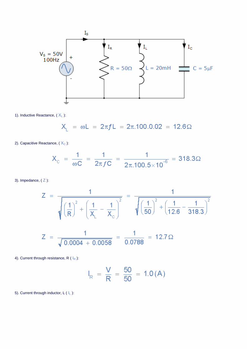
1). Inductive Reactance, ( XL ):

2). Capacitive Reactance, ( XC ):

3). Impedance, ( Z ):

4). Current through resistance, R ( IR ):

5). Current through inductor, L ( IL ):

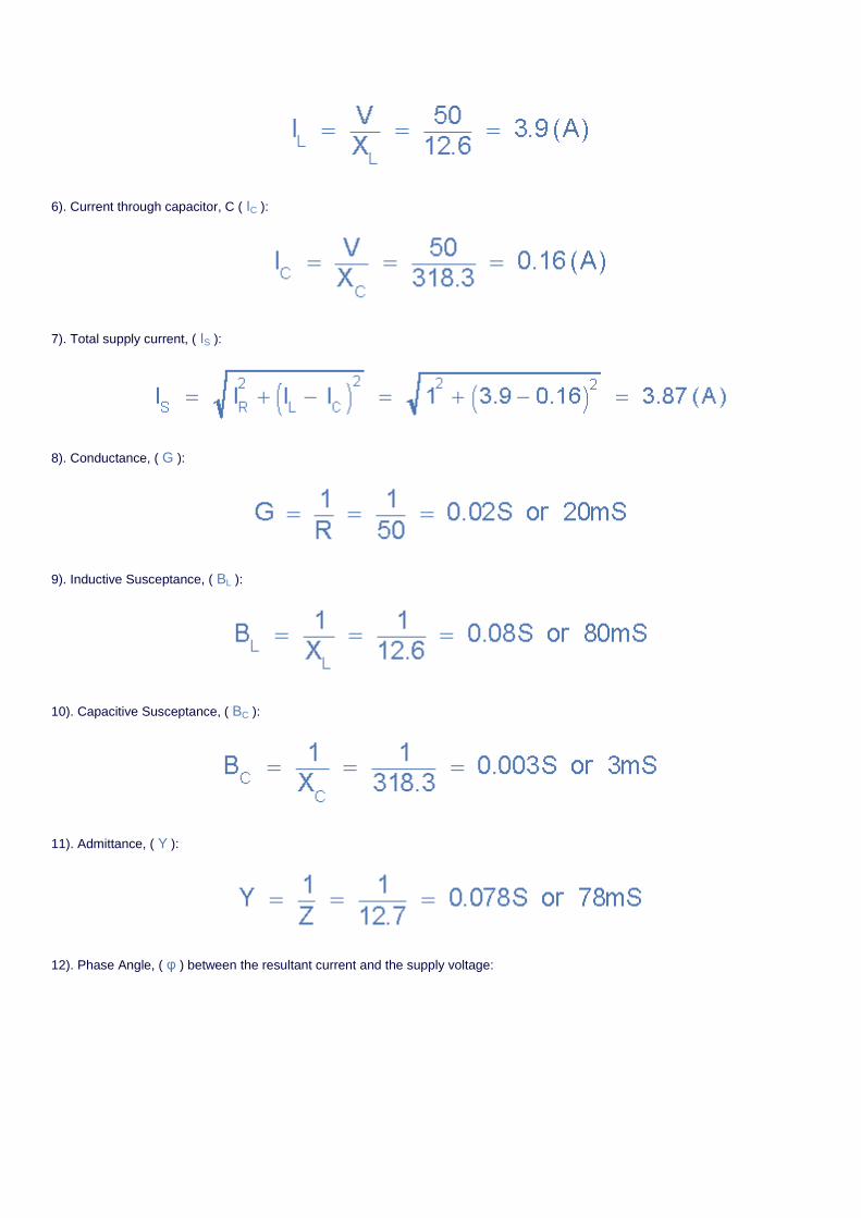
6). Current through capacitor, C ( IC ):

7). Total supply current, ( IS ):

8). Conductance, ( G ):

9). Inductive Susceptance, ( BL ):

10). Capacitive Susceptance, ( BC ):

11). Admittance, ( Y ):

12). Phase Angle, ( φ ) between the resultant current and the supply voltage:

Current and Admittance Triangles

Parallel RLC Circuit Summary

In a parallel RLC circuit containing a resistor, an inductor and a capacitor the circuit current IS is the phasor sum made up of three

components, IR, IL and IC with the supply voltage common to all three. Since the supply voltage is common to all three components it is

used as the horizontal reference when constructing a current triangle.

Parallel RLC networks can be analysed using vector diagrams just the same as with series RLC circuits. However, the analysis of

parallel RLC circuits is a little more mathematically difficult than for series RLC circuits when it contains two or more current branches.

So an AC parallel circuit can be easily analysed using the reciprocal of impedance called Admittance.

Admittance is the reciprocal of impedance given the symbol, Y. Like impedance, it is a complex quantity consisting of a real part and an

imaginary part. The real part is the reciprocal of resistance and is called Conductance, symbol Y while the imaginary part is the

reciprocal of reactance and is called Susceptance, symbol B and expressed in complex form as: Y = G + jB with the duality between

the two complex impedances being defined as:

Series Circuit Parallel Circuit

Voltage, (V) Current, (I)

Resistance, (R) Conductance, (G)

Reactance, (X) Susceptance, (B)

Impedance, (Z) Admittance, (Y)

As susceptance is the reciprocal of reactance, in an inductive circuit, inductive susceptance, BL will be negative in value and in a

capacitive circuit, capacitive susceptance, BC will be positive in value. The exact opposite to XL and XCrespectively.

We have seen so far that series and parallel RLC circuits contain both capacitive reactance and inductive reactance within the same

circuit. If we vary the frequency across these circuits there must become a point where the capacitive reactance value equals that of

the inductive reactance and therefore,XC = XL. The frequency point at which this occurs is called resonance and in the next tutorial we

will look at series resonance and how its presence alters the characteristics of the circuit.

Series Resonance Navigation

Tutorial: 11 of 12

--- Select a Tutorial Page ---

RESET

The Series Resonance Circuit

Thus far we have analysed the behaviour of a series RLC circuit whose source voltage is a fixed frequency steady state sinusoidal

supply. we have also seen that two or more sinusoidal signals can be combined using phasors providing that they have the same

frequency supply. But what would happen to the characteristics of the circuit if a supply voltage of fixed amplitude but of different

frequencies was applied to the circuit. Also what would the circuits "frequency response" behaviour be upon the two reactive

components due to this varying frequency.

In a series RLC circuit there becomes a frequency point were the inductive reactance of the inductor becomes equal in value to the

capacitive reactance of the capacitor. In other words,XL = XC. The point at which this occurs is called theResonant Frequency point, (

ƒr ) of the circuit, and as we are analysing a series RLC circuit this resonance frequency produces a Series Resonance.

Series Resonance circuits are one of the most important circuits used electrical and electronic circuits. They can be found in various

forms such as in AC mains filters, noise filters and also in radio and television tunning circuits producing a very selective tuning circuit

for the receiving of the different frequency channels. Consider the simple series RLC circuit below.

Series RLC Circuit

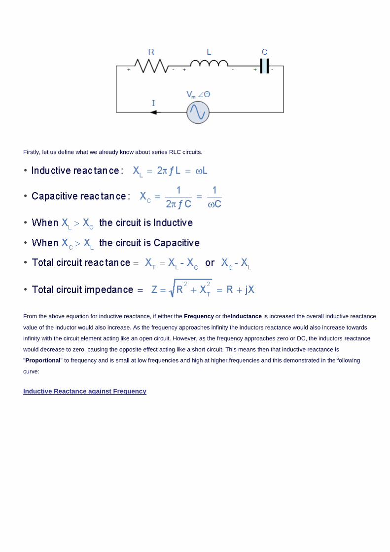
Firstly, let us define what we already know about series RLC circuits.

From the above equation for inductive reactance, if either the Frequency or theInductance is increased the overall inductive reactance

value of the inductor would also increase. As the frequency approaches infinity the inductors reactance would also increase towards

infinity with the circuit element acting like an open circuit. However, as the frequency approaches zero or DC, the inductors reactance

would decrease to zero, causing the opposite effect acting like a short circuit. This means then that inductive reactance is

"Proportional" to frequency and is small at low frequencies and high at higher frequencies and this demonstrated in the following

curve:

Inductive Reactance against Frequency

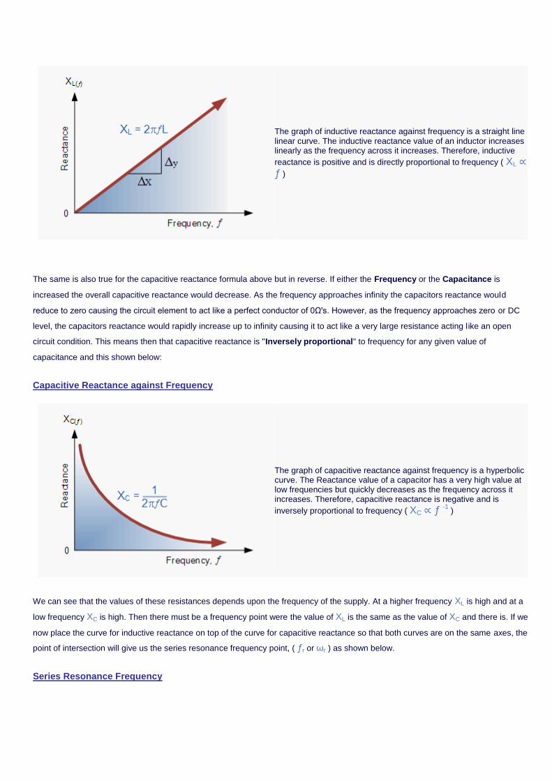
The graph of inductive reactance against frequency is a straight line linear curve. The inductive reactance value of an inductor increases linearly as the frequency across it increases. Therefore, inductive

reactance is positive and is directly proportional to frequency ( XL ∝ ƒ )

The same is also true for the capacitive reactance formula above but in reverse. If either the Frequency or the Capacitance is

increased the overall capacitive reactance would decrease. As the frequency approaches infinity the capacitors reactance would

reduce to zero causing the circuit element to act like a perfect conductor of 0Ω's. However, as the frequency approaches zero or DC

level, the capacitors reactance would rapidly increase up to infinity causing it to act like a very large resistance acting like an open

circuit condition. This means then that capacitive reactance is "Inversely proportional" to frequency for any given value of

capacitance and this shown below:

Capacitive Reactance against Frequency

The graph of capacitive reactance against frequency is a hyperbolic curve. The Reactance value of a capacitor has a very high value at low frequencies but quickly decreases as the frequency across it increases. Therefore, capacitive reactance is negative and is

inversely proportional to frequency ( XC ∝ ƒ -1 )

We can see that the values of these resistances depends upon the frequency of the supply. At a higher frequency XL is high and at a

low frequency XC is high. Then there must be a frequency point were the value of XL is the same as the value of XC and there is. If we

now place the curve for inductive reactance on top of the curve for capacitive reactance so that both curves are on the same axes, the

point of intersection will give us the series resonance frequency point, ( ƒr or ωr ) as shown below.

Series Resonance Frequency

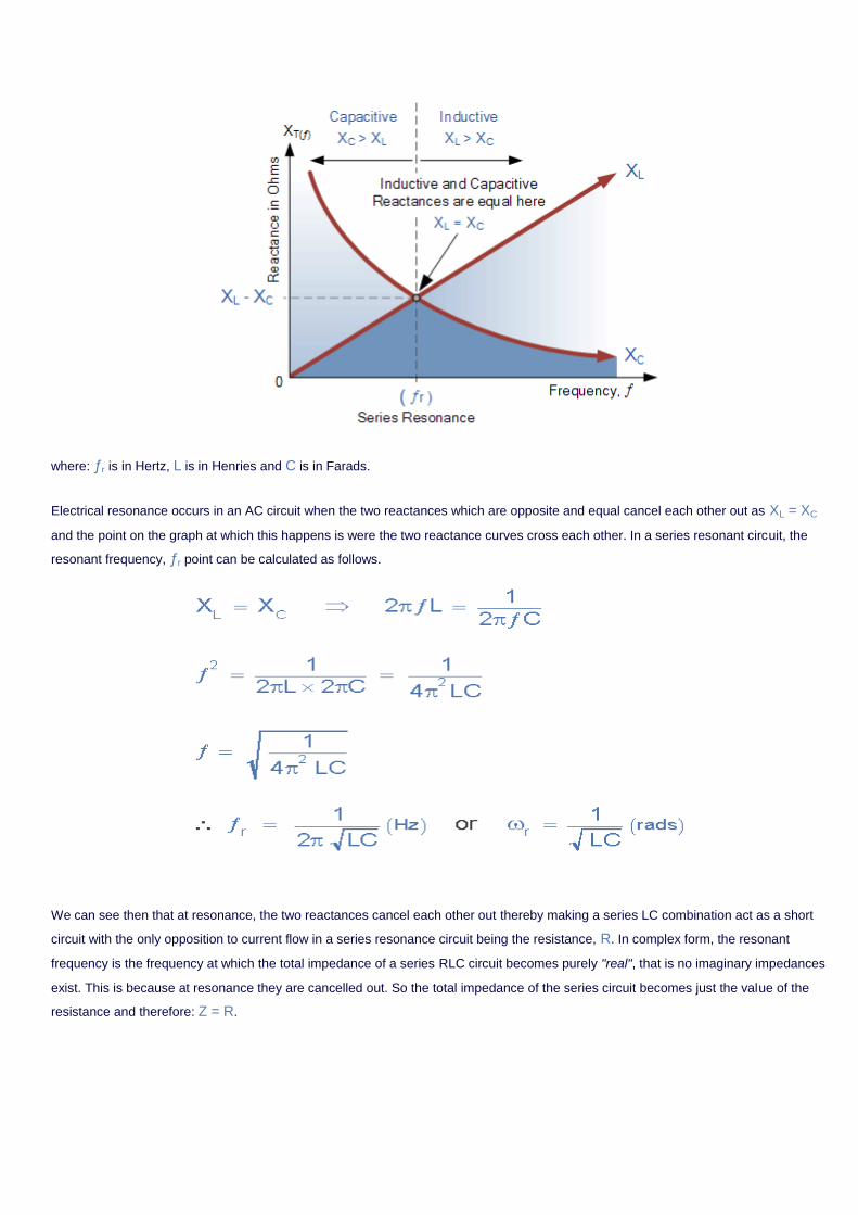
where: ƒr is in Hertz, L is in Henries and C is in Farads.

Electrical resonance occurs in an AC circuit when the two reactances which are opposite and equal cancel each other out as XL = XC

and the point on the graph at which this happens is were the two reactance curves cross each other. In a series resonant circuit, the

resonant frequency, ƒr point can be calculated as follows.

We can see then that at resonance, the two reactances cancel each other out thereby making a series LC combination act as a short

circuit with the only opposition to current flow in a series resonance circuit being the resistance, R. In complex form, the resonant

frequency is the frequency at which the total impedance of a series RLC circuit becomes purely "real", that is no imaginary impedances

exist. This is because at resonance they are cancelled out. So the total impedance of the series circuit becomes just the value of the

resistance and therefore: Z = R.

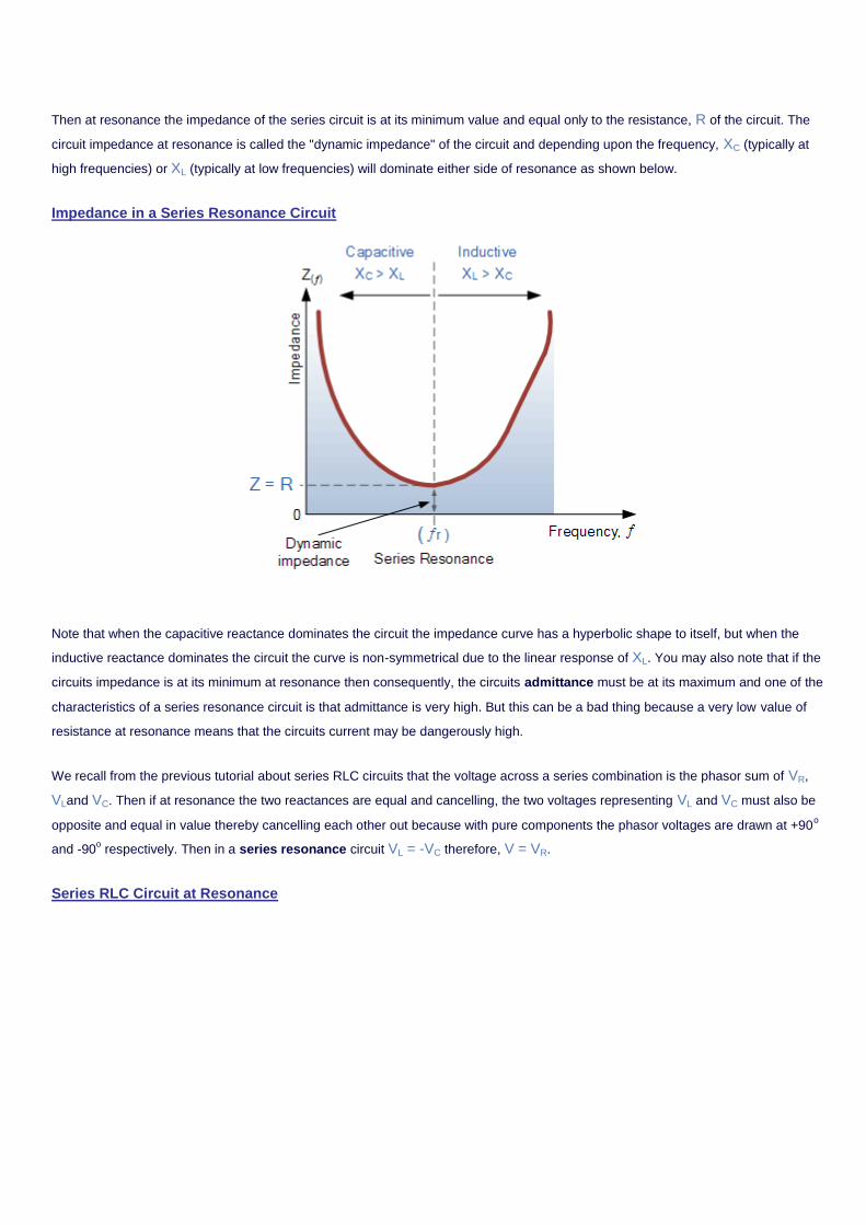
Then at resonance the impedance of the series circuit is at its minimum value and equal only to the resistance, R of the circuit. The

circuit impedance at resonance is called the "dynamic impedance" of the circuit and depending upon the frequency, XC (typically at

high frequencies) or XL (typically at low frequencies) will dominate either side of resonance as shown below.

Impedance in a Series Resonance Circuit

Note that when the capacitive reactance dominates the circuit the impedance curve has a hyperbolic shape to itself, but when the

inductive reactance dominates the circuit the curve is non-symmetrical due to the linear response of XL. You may also note that if the

circuits impedance is at its minimum at resonance then consequently, the circuits admittance must be at its maximum and one of the

characteristics of a series resonance circuit is that admittance is very high. But this can be a bad thing because a very low value of

resistance at resonance means that the circuits current may be dangerously high.

We recall from the previous tutorial about series RLC circuits that the voltage across a series combination is the phasor sum of VR,

VLand VC. Then if at resonance the two reactances are equal and cancelling, the two voltages representing VL and VC must also be

opposite and equal in value thereby cancelling each other out because with pure components the phasor voltages are drawn at +90o

and -90o respectively. Then in a series resonance circuit VL = -VC therefore, V = VR.

Series RLC Circuit at Resonance

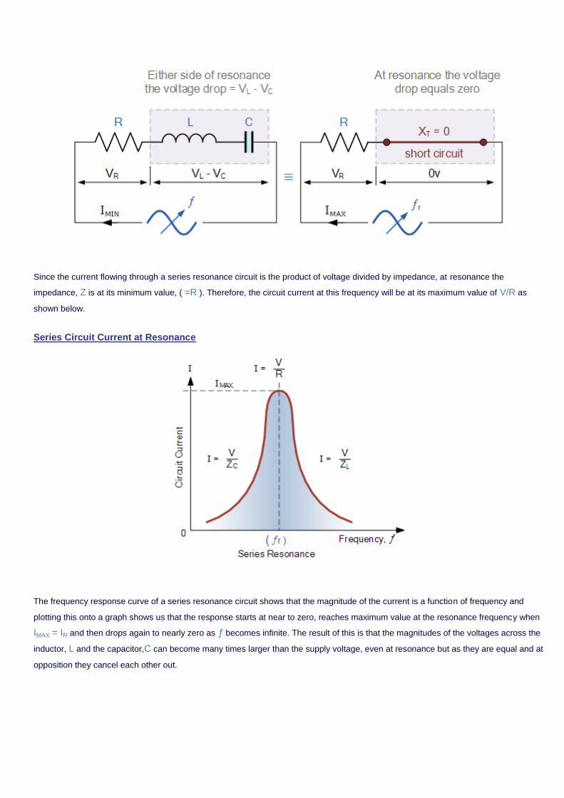
Since the current flowing through a series resonance circuit is the product of voltage divided by impedance, at resonance the

impedance, Z is at its minimum value, ( =R ). Therefore, the circuit current at this frequency will be at its maximum value of V/R as

shown below.

Series Circuit Current at Resonance

The frequency response curve of a series resonance circuit shows that the magnitude of the current is a function of frequency and

plotting this onto a graph shows us that the response starts at near to zero, reaches maximum value at the resonance frequency when

IMAX = IR and then drops again to nearly zero as ƒ becomes infinite. The result of this is that the magnitudes of the voltages across the

inductor, L and the capacitor,C can become many times larger than the supply voltage, even at resonance but as they are equal and at

opposition they cancel each other out.

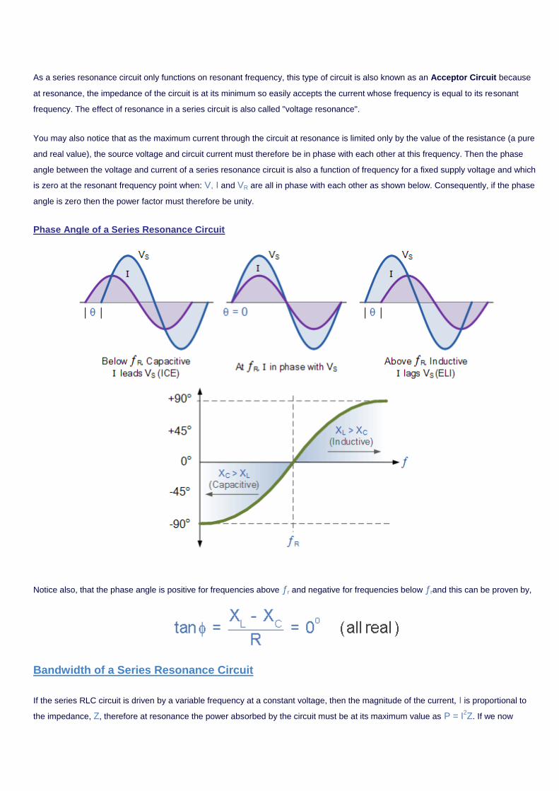
As a series resonance circuit only functions on resonant frequency, this type of circuit is also known as an Acceptor Circuit because

at resonance, the impedance of the circuit is at its minimum so easily accepts the current whose frequency is equal to its resonant

frequency. The effect of resonance in a series circuit is also called "voltage resonance".

You may also notice that as the maximum current through the circuit at resonance is limited only by the value of the resistance (a pure

and real value), the source voltage and circuit current must therefore be in phase with each other at this frequency. Then the phase

angle between the voltage and current of a series resonance circuit is also a function of frequency for a fixed supply voltage and which

is zero at the resonant frequency point when: V, I and VR are all in phase with each other as shown below. Consequently, if the phase

angle is zero then the power factor must therefore be unity.

Phase Angle of a Series Resonance Circuit

Notice also, that the phase angle is positive for frequencies above ƒr and negative for frequencies below ƒrand this can be proven by,

Bandwidth of a Series Resonance Circuit

If the series RLC circuit is driven by a variable frequency at a constant voltage, then the magnitude of the current, I is proportional to

the impedance, Z, therefore at resonance the power absorbed by the circuit must be at its maximum value as P = I2Z. If we now

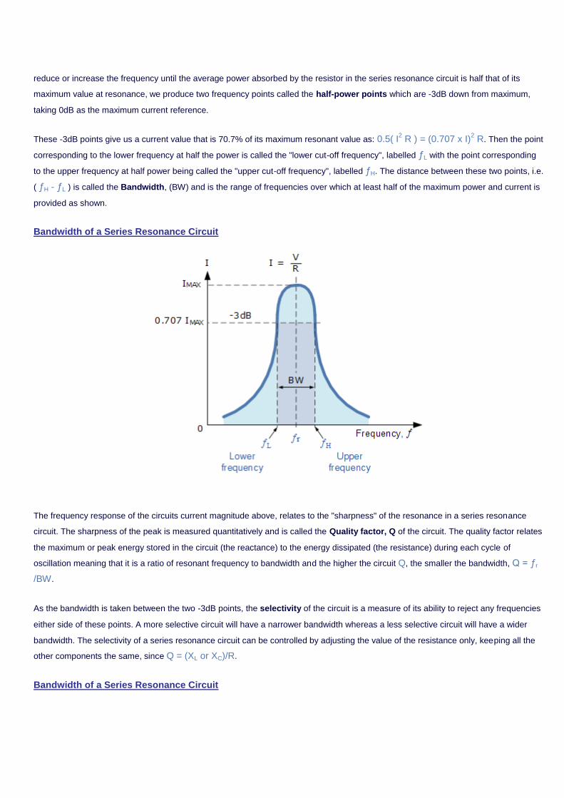
reduce or increase the frequency until the average power absorbed by the resistor in the series resonance circuit is half that of its

maximum value at resonance, we produce two frequency points called the half-power points which are -3dB down from maximum,

taking 0dB as the maximum current reference.

These -3dB points give us a current value that is 70.7% of its maximum resonant value as: 0.5( I2 R ) = (0.707 x I)

2 R. Then the point

corresponding to the lower frequency at half the power is called the "lower cut-off frequency", labelled ƒL with the point corresponding

to the upper frequency at half power being called the "upper cut-off frequency", labelled ƒH. The distance between these two points, i.e.

( ƒH - ƒL ) is called the Bandwidth, (BW) and is the range of frequencies over which at least half of the maximum power and current is

provided as shown.

Bandwidth of a Series Resonance Circuit

The frequency response of the circuits current magnitude above, relates to the "sharpness" of the resonance in a series resonance

circuit. The sharpness of the peak is measured quantitatively and is called the Quality factor, Q of the circuit. The quality factor relates

the maximum or peak energy stored in the circuit (the reactance) to the energy dissipated (the resistance) during each cycle of

oscillation meaning that it is a ratio of resonant frequency to bandwidth and the higher the circuit Q, the smaller the bandwidth, Q = ƒr

/BW.

As the bandwidth is taken between the two -3dB points, the selectivity of the circuit is a measure of its ability to reject any frequencies

either side of these points. A more selective circuit will have a narrower bandwidth whereas a less selective circuit will have a wider

bandwidth. The selectivity of a series resonance circuit can be controlled by adjusting the value of the resistance only, keeping all the

other components the same, since Q = (XL or XC)/R.

Bandwidth of a Series Resonance Circuit

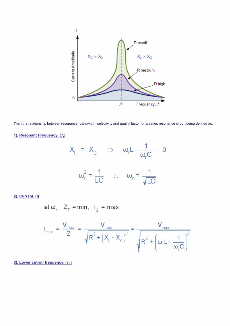
Then the relationship between resonance, bandwidth, selectivity and quality factor for a series resonance circuit being defined as:

1). Resonant Frequency, (ƒr)

2). Current, (I)

3). Lower cut-off frequency, (ƒL)

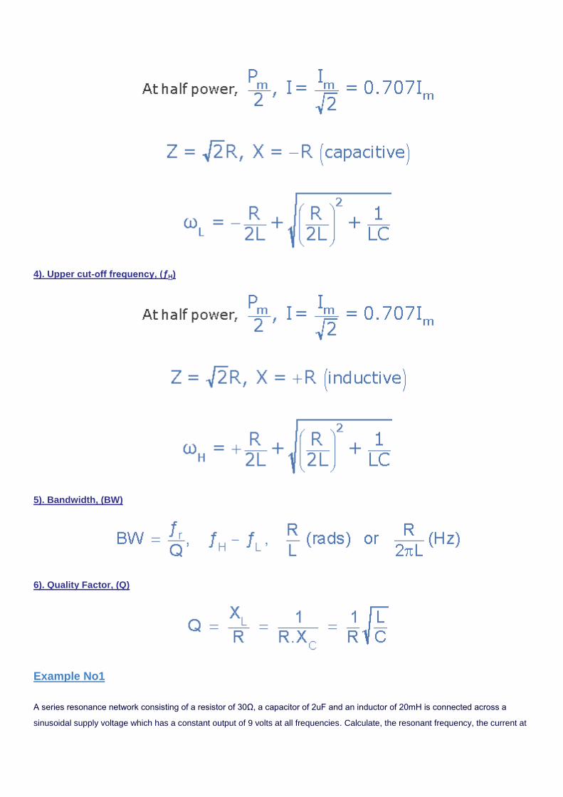
4). Upper cut-off frequency, (ƒH)

5). Bandwidth, (BW)

6). Quality Factor, (Q)

Example No1

A series resonance network consisting of a resistor of 30Ω, a capacitor of 2uF and an inductor of 20mH is connected across a

sinusoidal supply voltage which has a constant output of 9 volts at all frequencies. Calculate, the resonant frequency, the current at

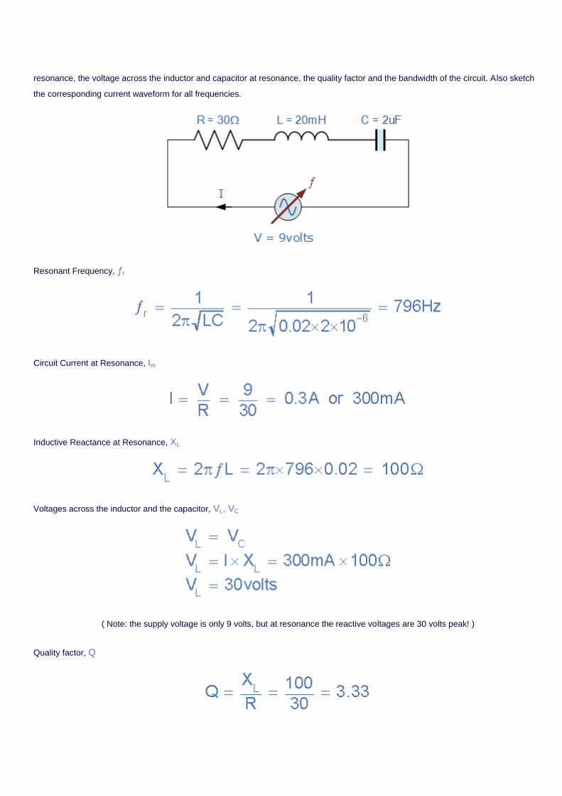
resonance, the voltage across the inductor and capacitor at resonance, the quality factor and the bandwidth of the circuit. Also sketch

the corresponding current waveform for all frequencies.

Resonant Frequency, ƒr

Circuit Current at Resonance, Im

Inductive Reactance at Resonance, XL

Voltages across the inductor and the capacitor, VL, VC

( Note: the supply voltage is only 9 volts, but at resonance the reactive voltages are 30 volts peak! )

Quality factor, Q

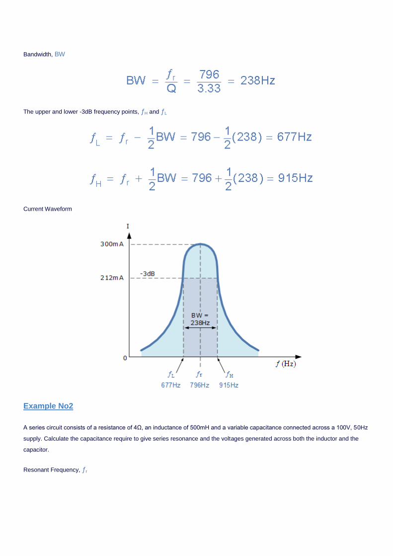
Bandwidth, BW

The upper and lower -3dB frequency points, ƒH and ƒL

Current Waveform

Example No2

A series circuit consists of a resistance of 4Ω, an inductance of 500mH and a variable capacitance connected across a 100V, 50Hz

supply. Calculate the capacitance require to give series resonance and the voltages generated across both the inductor and the

capacitor.

Resonant Frequency, ƒr

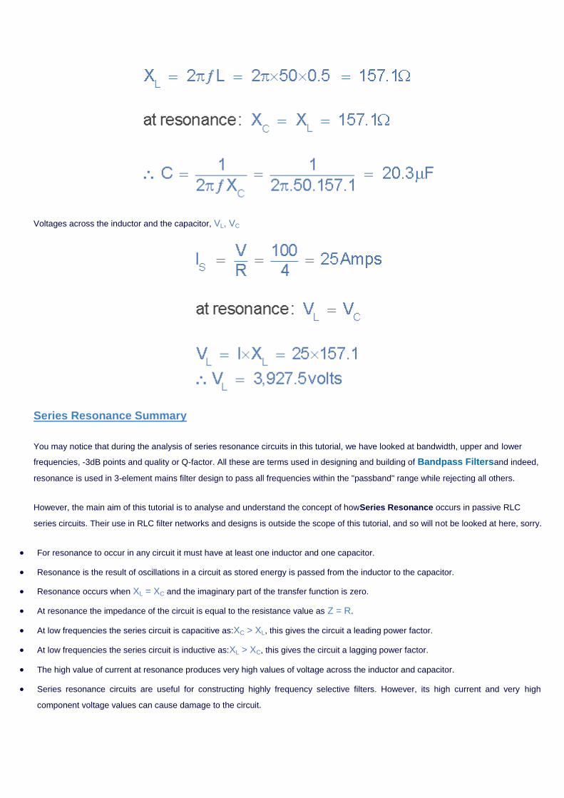
Voltages across the inductor and the capacitor, VL, VC

Series Resonance Summary

You may notice that during the analysis of series resonance circuits in this tutorial, we have looked at bandwidth, upper and lower

frequencies, -3dB points and quality or Q-factor. All these are terms used in designing and building of Bandpass Filtersand indeed,

resonance is used in 3-element mains filter design to pass all frequencies within the "passband" range while rejecting all others.

However, the main aim of this tutorial is to analyse and understand the concept of howSeries Resonance occurs in passive RLC

series circuits. Their use in RLC filter networks and designs is outside the scope of this tutorial, and so will not be looked at here, sorry.

For resonance to occur in any circuit it must have at least one inductor and one capacitor.

Resonance is the result of oscillations in a circuit as stored energy is passed from the inductor to the capacitor.

Resonance occurs when XL = XC and the imaginary part of the transfer function is zero.

At resonance the impedance of the circuit is equal to the resistance value as Z = R.

At low frequencies the series circuit is capacitive as:XC > XL, this gives the circuit a leading power factor.

At low frequencies the series circuit is inductive as:XL > XC, this gives the circuit a lagging power factor.

The high value of current at resonance produces very high values of voltage across the inductor and capacitor.

Series resonance circuits are useful for constructing highly frequency selective filters. However, its high current and very high

component voltage values can cause damage to the circuit.

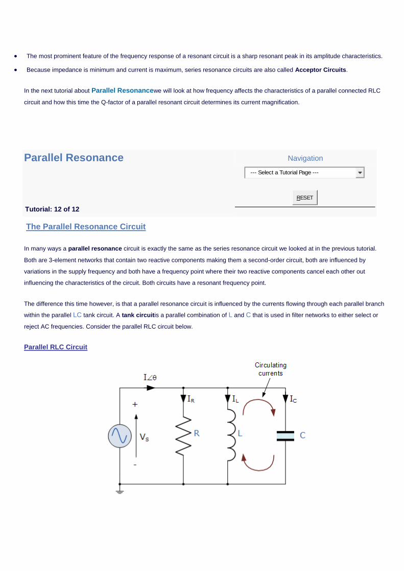
The most prominent feature of the frequency response of a resonant circuit is a sharp resonant peak in its amplitude characteristics.

Because impedance is minimum and current is maximum, series resonance circuits are also called Acceptor Circuits.

In the next tutorial about Parallel Resonancewe will look at how frequency affects the characteristics of a parallel connected RLC

circuit and how this time the Q-factor of a parallel resonant circuit determines its current magnification.

Parallel Resonance Navigation

Tutorial: 12 of 12

--- Select a Tutorial Page ---

RESET

The Parallel Resonance Circuit

In many ways a parallel resonance circuit is exactly the same as the series resonance circuit we looked at in the previous tutorial.

Both are 3-element networks that contain two reactive components making them a second-order circuit, both are influenced by

variations in the supply frequency and both have a frequency point where their two reactive components cancel each other out

influencing the characteristics of the circuit. Both circuits have a resonant frequency point.

The difference this time however, is that a parallel resonance circuit is influenced by the currents flowing through each parallel branch

within the parallel LC tank circuit. A tank circuitis a parallel combination of L and C that is used in filter networks to either select or

reject AC frequencies. Consider the parallel RLC circuit below.

Parallel RLC Circuit

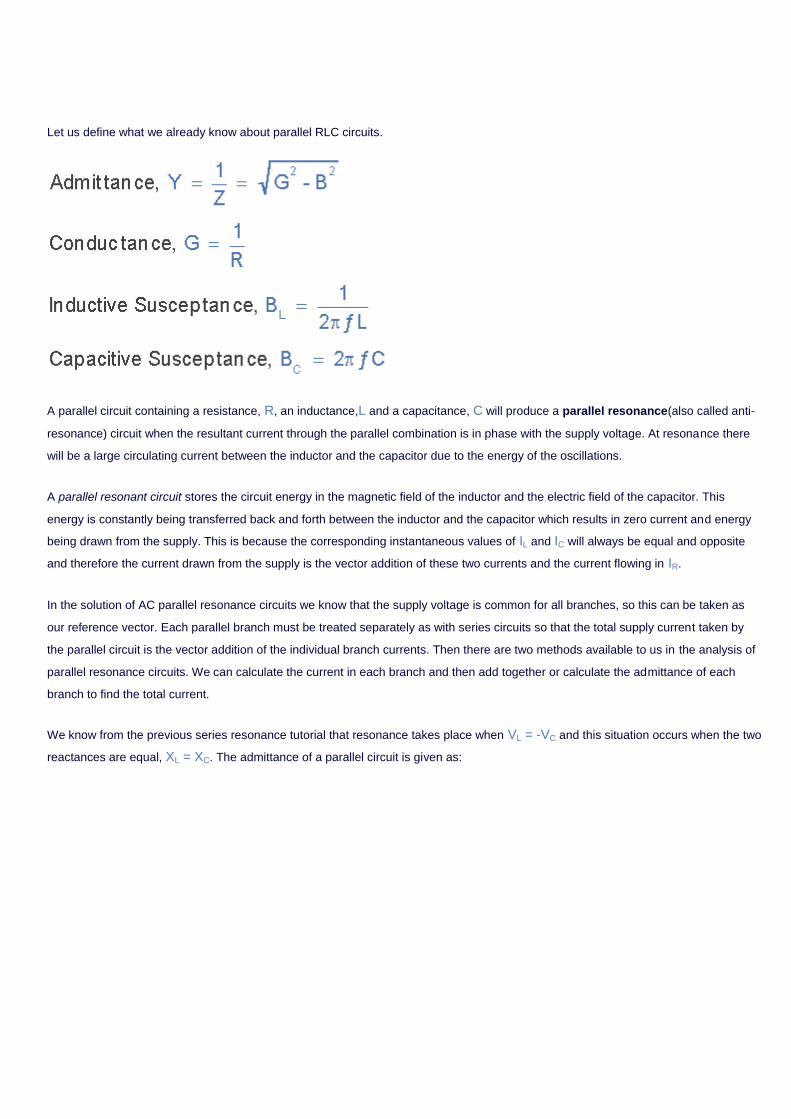
Let us define what we already know about parallel RLC circuits.

A parallel circuit containing a resistance, R, an inductance,L and a capacitance, C will produce a parallel resonance(also called anti-

resonance) circuit when the resultant current through the parallel combination is in phase with the supply voltage. At resonance there

will be a large circulating current between the inductor and the capacitor due to the energy of the oscillations.

A parallel resonant circuit stores the circuit energy in the magnetic field of the inductor and the electric field of the capacitor. This

energy is constantly being transferred back and forth between the inductor and the capacitor which results in zero current and energy

being drawn from the supply. This is because the corresponding instantaneous values of IL and IC will always be equal and opposite

and therefore the current drawn from the supply is the vector addition of these two currents and the current flowing in IR.

In the solution of AC parallel resonance circuits we know that the supply voltage is common for all branches, so this can be taken as

our reference vector. Each parallel branch must be treated separately as with series circuits so that the total supply current taken by

the parallel circuit is the vector addition of the individual branch currents. Then there are two methods available to us in the analysis of

parallel resonance circuits. We can calculate the current in each branch and then add together or calculate the admittance of each

branch to find the total current.

We know from the previous series resonance tutorial that resonance takes place when VL = -VC and this situation occurs when the two

reactances are equal, XL = XC. The admittance of a parallel circuit is given as:

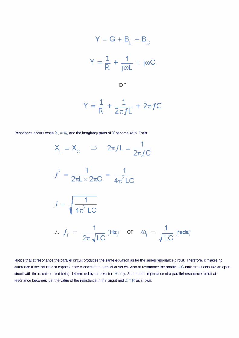
Resonance occurs when XL = XC and the imaginary parts of Y become zero. Then:

Notice that at resonance the parallel circuit produces the same equation as for the series resonance circuit. Therefore, it makes no

difference if the inductor or capacitor are connected in parallel or series. Also at resonance the parallel LC tank circuit acts like an open

circuit with the circuit current being determined by the resistor, R only. So the total impedance of a parallel resonance circuit at

resonance becomes just the value of the resistance in the circuit and Z = R as shown.

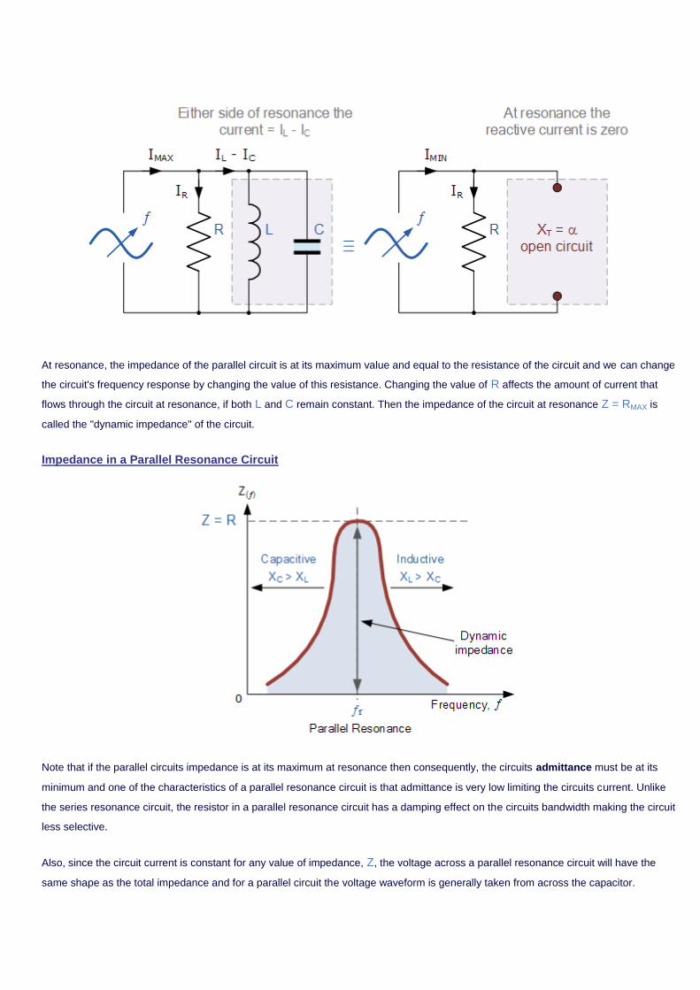
At resonance, the impedance of the parallel circuit is at its maximum value and equal to the resistance of the circuit and we can change

the circuit's frequency response by changing the value of this resistance. Changing the value of R affects the amount of current that

flows through the circuit at resonance, if both L and C remain constant. Then the impedance of the circuit at resonance Z = RMAX is

called the "dynamic impedance" of the circuit.

Impedance in a Parallel Resonance Circuit

Note that if the parallel circuits impedance is at its maximum at resonance then consequently, the circuits admittance must be at its

minimum and one of the characteristics of a parallel resonance circuit is that admittance is very low limiting the circuits current. Unlike

the series resonance circuit, the resistor in a parallel resonance circuit has a damping effect on the circuits bandwidth making the circuit

less selective.

Also, since the circuit current is constant for any value of impedance, Z, the voltage across a parallel resonance circuit will have the

same shape as the total impedance and for a parallel circuit the voltage waveform is generally taken from across the capacitor.

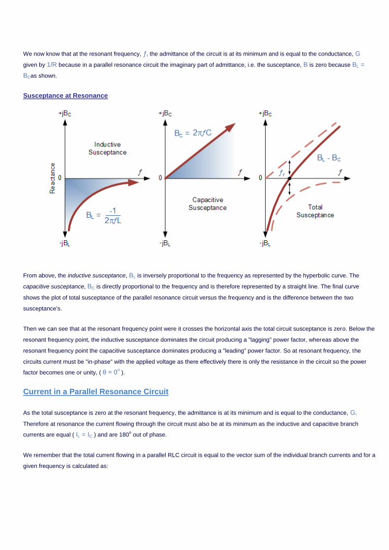
We now know that at the resonant frequency, ƒr the admittance of the circuit is at its minimum and is equal to the conductance, G

given by 1/R because in a parallel resonance circuit the imaginary part of admittance, i.e. the susceptance, B is zero because BL =

BCas shown.

Susceptance at Resonance

From above, the inductive susceptance, BL is inversely proportional to the frequency as represented by the hyperbolic curve. The

capacitive susceptance, BC is directly proportional to the frequency and is therefore represented by a straight line. The final curve

shows the plot of total susceptance of the parallel resonance circuit versus the frequency and is the difference between the two

susceptance's.

Then we can see that at the resonant frequency point were it crosses the horizontal axis the total circuit susceptance is zero. Below the

resonant frequency point, the inductive susceptance dominates the circuit producing a "lagging" power factor, whereas above the

resonant frequency point the capacitive susceptance dominates producing a "leading" power factor. So at resonant frequency, the

circuits current must be "in-phase" with the applied voltage as there effectively there is only the resistance in the circuit so the power

factor becomes one or unity, ( θ = 0o ).

Current in a Parallel Resonance Circuit

As the total susceptance is zero at the resonant frequency, the admittance is at its minimum and is equal to the conductance, G.

Therefore at resonance the current flowing through the circuit must also be at its minimum as the inductive and capacitive branch

currents are equal ( IL = IC ) and are 180o out of phase.

We remember that the total current flowing in a parallel RLC circuit is equal to the vector sum of the individual branch currents and for a

given frequency is calculated as:

At resonance, currents IL and IL are equal and cancelling giving a net reactive current equal to zero. Then at resonance the above

equation becomes.

Since the current flowing through a parallel resonance circuit is the product of voltage divided by impedance, at resonance the

impedance, Z is at its maximum value, ( =R ). Therefore, the circuit current at this frequency will be at its minimum value of V/R and

the graph of current against frequency for a parallel resonance circuit is given as.

Parallel Circuit Current at Resonance

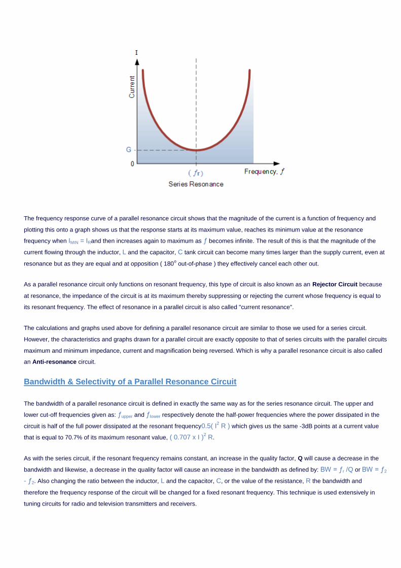
The frequency response curve of a parallel resonance circuit shows that the magnitude of the current is a function of frequency and

plotting this onto a graph shows us that the response starts at its maximum value, reaches its minimum value at the resonance

frequency when IMIN = IRand then increases again to maximum as ƒ becomes infinite. The result of this is that the magnitude of the

current flowing through the inductor, L and the capacitor, C tank circuit can become many times larger than the supply current, even at

resonance but as they are equal and at opposition ( 180o out-of-phase ) they effectively cancel each other out.

As a parallel resonance circuit only functions on resonant frequency, this type of circuit is also known as an Rejector Circuit because

at resonance, the impedance of the circuit is at its maximum thereby suppressing or rejecting the current whose frequency is equal to

its resonant frequency. The effect of resonance in a parallel circuit is also called "current resonance".

The calculations and graphs used above for defining a parallel resonance circuit are similar to those we used for a series circuit.

However, the characteristics and graphs drawn for a parallel circuit are exactly opposite to that of series circuits with the parallel circuits

maximum and minimum impedance, current and magnification being reversed. Which is why a parallel resonance circuit is also called

an Anti-resonance circuit.

Bandwidth & Selectivity of a Parallel Resonance Circuit

The bandwidth of a parallel resonance circuit is defined in exactly the same way as for the series resonance circuit. The upper and

lower cut-off frequencies given as: ƒupper and ƒlower respectively denote the half-power frequencies where the power dissipated in the

circuit is half of the full power dissipated at the resonant frequency0.5( I2 R ) which gives us the same -3dB points at a current value

that is equal to 70.7% of its maximum resonant value, ( 0.707 x I )2 R.

As with the series circuit, if the resonant frequency remains constant, an increase in the quality factor, Q will cause a decrease in the

bandwidth and likewise, a decrease in the quality factor will cause an increase in the bandwidth as defined by: BW = ƒr /Q or BW = ƒ2

- ƒ2. Also changing the ratio between the inductor, L and the capacitor, C, or the value of the resistance, R the bandwidth and

therefore the frequency response of the circuit will be changed for a fixed resonant frequency. This technique is used extensively in

tuning circuits for radio and television transmitters and receivers.

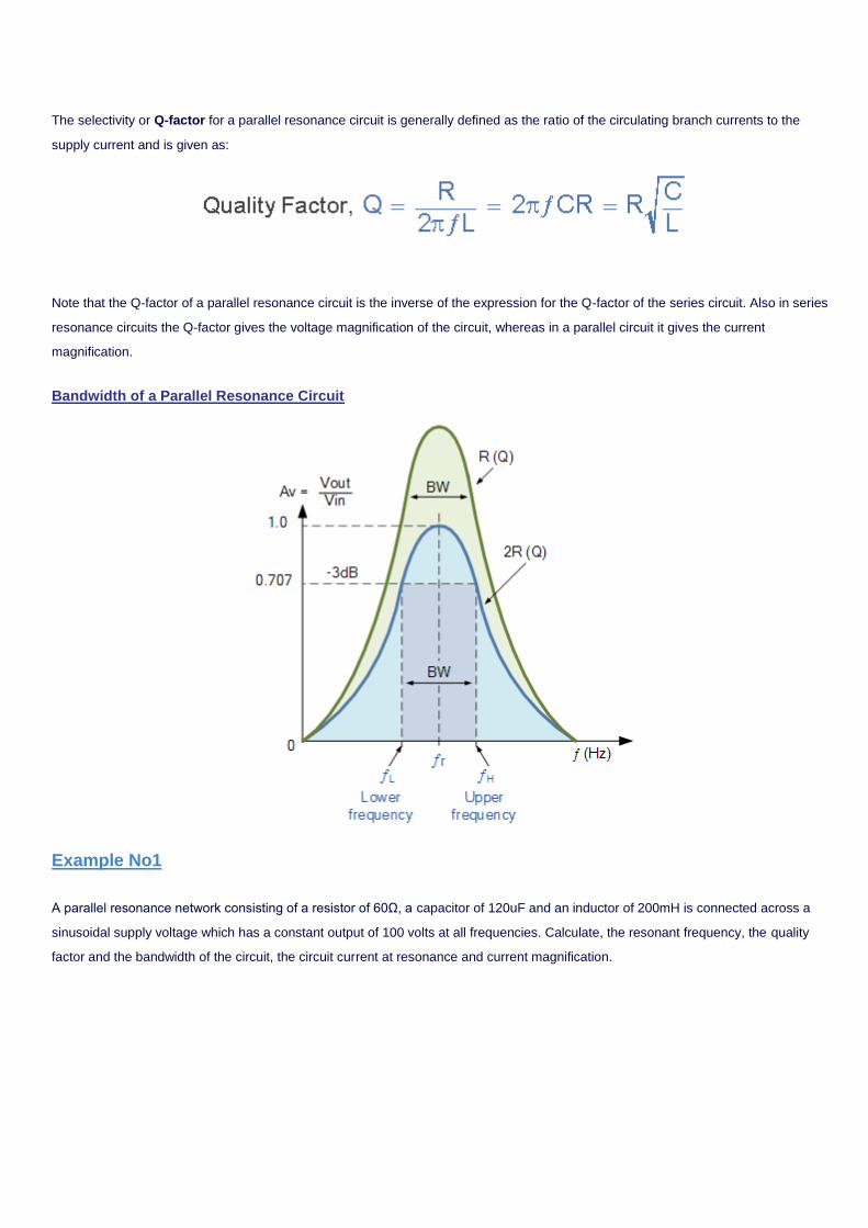
The selectivity or Q-factor for a parallel resonance circuit is generally defined as the ratio of the circulating branch currents to the

supply current and is given as:

Note that the Q-factor of a parallel resonance circuit is the inverse of the expression for the Q-factor of the series circuit. Also in series

resonance circuits the Q-factor gives the voltage magnification of the circuit, whereas in a parallel circuit it gives the current

magnification.

Bandwidth of a Parallel Resonance Circuit

Example No1

A parallel resonance network consisting of a resistor of 60Ω, a capacitor of 120uF and an inductor of 200mH is connected across a

sinusoidal supply voltage which has a constant output of 100 volts at all frequencies. Calculate, the resonant frequency, the quality

factor and the bandwidth of the circuit, the circuit current at resonance and current magnification.

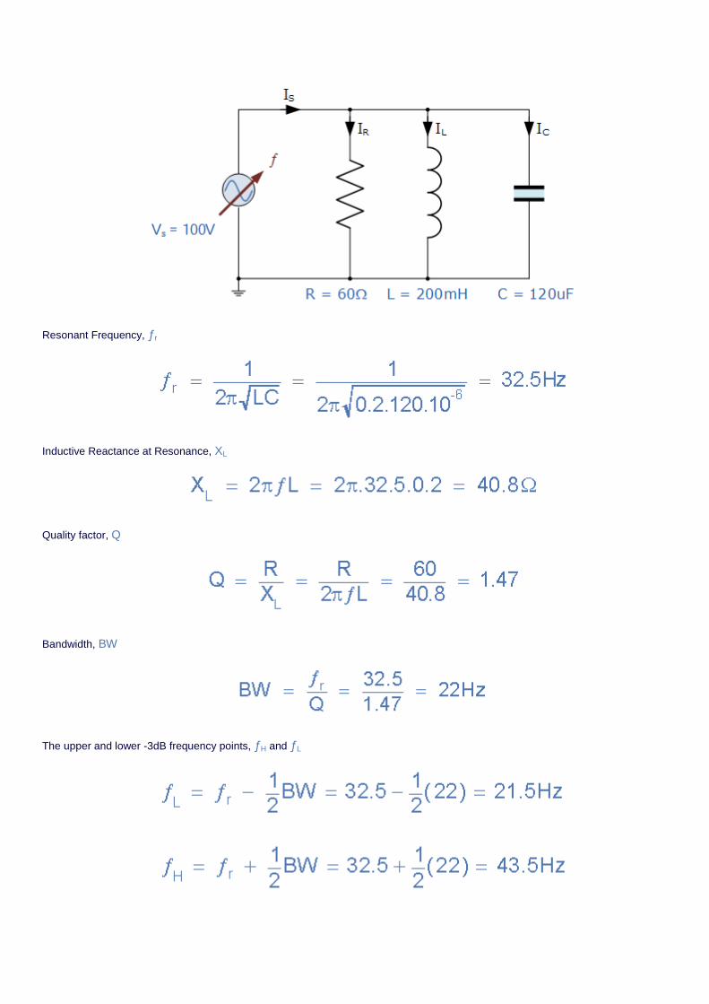
Resonant Frequency, ƒr

Inductive Reactance at Resonance, XL

Quality factor, Q

Bandwidth, BW

The upper and lower -3dB frequency points, ƒH and ƒL

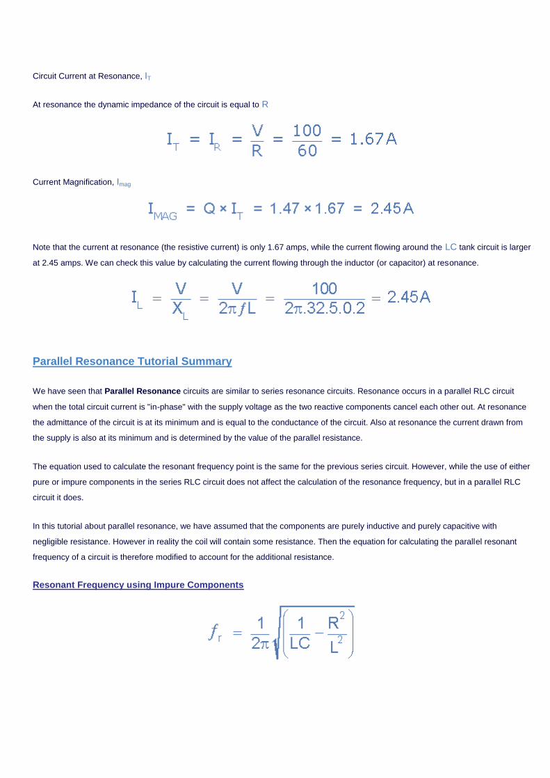
Circuit Current at Resonance, IT

At resonance the dynamic impedance of the circuit is equal to R

Current Magnification, Imag

Note that the current at resonance (the resistive current) is only 1.67 amps, while the current flowing around the LC tank circuit is larger

at 2.45 amps. We can check this value by calculating the current flowing through the inductor (or capacitor) at resonance.

Parallel Resonance Tutorial Summary

We have seen that Parallel Resonance circuits are similar to series resonance circuits. Resonance occurs in a parallel RLC circuit

when the total circuit current is "in-phase" with the supply voltage as the two reactive components cancel each other out. At resonance

the admittance of the circuit is at its minimum and is equal to the conductance of the circuit. Also at resonance the current drawn from

the supply is also at its minimum and is determined by the value of the parallel resistance.

The equation used to calculate the resonant frequency point is the same for the previous series circuit. However, while the use of either

pure or impure components in the series RLC circuit does not affect the calculation of the resonance frequency, but in a parallel RLC

circuit it does.

In this tutorial about parallel resonance, we have assumed that the components are purely inductive and purely capacitive with

negligible resistance. However in reality the coil will contain some resistance. Then the equation for calculating the parallel resonant

frequency of a circuit is therefore modified to account for the additional resistance.

Resonant Frequency using Impure Components